DAY OF THE WEEK EFFECT AND BOND MARKET RETURNS AT THENAIROBI SECURITIES EXCHANGE

BY MURIGU PERIS WANGUI

D61/60590/2013

A RESEARCH PROJECT SUBMITTED IN PARTIAL FULFILMENT OFTHE REQUIREMENTS FOR THE AWARD OF THE DEGREE OF MASTEROF BUSINESS ADMINISTRATION, UNIVERSITY OF NAIROBI

i

NOVEMBER 2014

ii

DECLARATION

This research project is my original work and has never been

presented for the award of a degree in any other university.

Sign:…………………………………….. Date:…………………………………..

Name: Murigu Peris Wangui

Adm. No.: D61/60590/2013

This research project has been submitted for examination with my

approval as the University

Supervisor;

Sign:…………………………………….. Date:…………………………………..

Mr. James Ng’ang’a

School of Business,

Department of Finance and Accounting,

University of Nairobi.

iii

iv

ACKNOWLEDGMENTS

It has been an exciting and instructive study period at the

University of Nairobi and I feel privileged to have had the

opportunity to carry out this study as a demonstration of the

knowledge gained during the period studying for my master’s

degree. With these acknowledgments, it would be impossible not to

remember those who in one way or another, directly or indirectly,

have played a role in the realization of this research project.

Let me, therefore, thank them all equally.

First, I am indebted to the all-powerful GOD for all the

blessings he showered on me and for being with me throughout the

study. I am deeply obliged to my supervisor for his exemplary

guidance and support without whose help; this project would not

have been a success. Finally, yet importantly, I take this

opportunity to express my deep gratitude to my loving family, and

friends who are a constant source of motivation and for their

never ending support and encouragement during this project.

v

DEDICATION

This project is dedicated to my dear parents Mr. and Mrs. Murigu,

my brothers George and Brian and to all my friends. I am indeed

indebted for the invaluable support and encouragement during the

course of my studies.

vi

vii

ABSTRACT

The objective of the study was to find out whether there exists arelationship between bonds returns and the day of the week at theNairobi Securities Exchange (NSE). It also sought to determine if there

is a significant difference in bond returns for all the five trading days. Therelationship between information and bond prices is explained bythe market efficiency. By the day of week effect, the investorwill consider the mean of return for different days. In adecision making process, a rational financial decision maker musttake into account not only returns but also the variance andvolatility of returns. The underlying constituents of the bondmarket are based on Kenyan Government Securities quoted on theNSE with maturity levels of more than one year and notionalamounts above KES5 billion. The bonds market in Kenya involvesboth the treasury and corporate bonds. The study was based on thecorporate bonds issued at the Nairobi Securities Exchange. Adescriptive research design was used in the study. It involvedgathering daily bond prices from the Nairobi Stock Exchange andanalyzing the data statistically to determine the existence ofthe day of the week effect on bond returns at the NSE. Thepopulation of interest in the study consisted of eleven firmswhich had issued bonds at the NSE as at 31st December 2013. Theirmean returns were used to investigate the relationship betweenthe day of the week and bond returns at the NSE. The datacomprised of the daily bond prices. The results show that there is asignificant relationship between the dependent variable which is the bondmarket return and independent variables which are the five days of theweek. From the analysis, we can conclude that Tuesday had the highestreturn than any other day of the week. Wednesday on the other hand, hadthe lowest negative return compared to other days. The research findingsalso indicate that there is little bond return volatility at the NSE as judgedby the distribution. The findings support that there is potential advantage

viii

to investors due to the day of the week effect anomaly is present in theKenyan bond market.

TABLE OF CONTENTS

DECLARATION...................................................ii

ACKNOWLEDGMENTS..............................................iii

DEDICATION....................................................iv

ABSTRACT.......................................................v

LIST OF TABLES................................................ix

LIST OF FIGURES...............................................ix

LIST OF ABBREVIATIONS..........................................x

CHAPTER ONE....................................................1

INTRODUCTION...................................................1

1.1 Background of the Study...................................1

1.1.1 Day of the Week Effect................................2

1.1.2 Bonds Returns.........................................3

ix

1.1.3 Day-of-the-Week Effect and Bonds Returns..............4

1.1.4 Nairobi Securities Exchange...........................6

1.2 Motivation for the Study..................................7

1.3 Research Problem..........................................7

1.4 Objective of the Study....................................9

1.5 Value of the Study........................................9

1.5.1 Academicians..........................................9

1.5.2 Investors.............................................9

1.5.3 Securities Market Regulators..........................9

1.5.4 Securities Brokers and Dealers.......................10

CHAPTER TWO...................................................11

LITERATURE REVIEW.............................................11

2.1 Introduction.............................................11

2.2. Efficient Market Hypothesis.............................11

2.3 Behavioral Finance Theory................................12

2.4 Determinants of Bonds Returns............................13

2.4.1 Issue Size...........................................13

2.4.2 Age of Bonds.........................................14

2.4.3 Interest Rate Risk...................................14

2.4.4 Credit Risk..........................................14

2.4.5 Equity Trading Volume and Return.....................15

2.4.6 Equity Market Conditions.............................15

2.5 Empirical Review.........................................15

2.5.1 Calendar Anomalies in Fixed Income Instruments.......15

x

2.5.2 Calendar Anomalies at the Nairobi Securities Exchange 18

2.6 Conclusion...............................................19

CHAPTER THREE.................................................20

RESEARCH METHODOLOGY..........................................20

3.1 Introduction.............................................20

3.2 Research Design..........................................20

3.3 Population...............................................21

3.4 Data Collection..........................................21

3.5 Data Analysis............................................21

CHAPTER FOUR..................................................24

DATA ANALYSIS, RESULTS AND DISCUSSION.........................24

4.1 Introduction.............................................24

4.2 Descriptive Statistics...................................24

4.3 Normality Test...........................................25

4.3.1 Multicollinearity – Correlation Matrix...............27

4.4 Regression Analysis......................................29

4.5 Discussions..............................................32

CHAPTER FIVE..................................................35

SUMMARY, CONCLUSION AND RECOMMENDATIONS.......................35

5.1 Introduction.............................................35

5.2 Summary..................................................35

5.3 Conclusion.................................................35

5.4 Recommendations...........................................36

5.5 Limitations of the Study......................................36

xi

5.6 Suggestions for Further Research..............................36

REFERENCES....................................................38

APPENDIX......................................................48

Appendix 1: Corporate Bonds Traded at the NSE................48

Appendix 2: Average Bond Returns.............................49

xii

LIST OF TABLES Page

Table 4.1 Descriptive Statistics 24

Table 4.2 Normality Test 26

Table 4.3 Correlation Matrix 27

Table 4.4 Multi-Collinearity Test 28

Table 4.5 Model Summary 29

Table 4.6 Analysis of Variance 30

Table 4.7 Models Coefficients 30

LIST OF FIGURES Page

Figure 4.1 P-P Plot 32

Figure 4.2 Day of the Week Trend 33

xiii

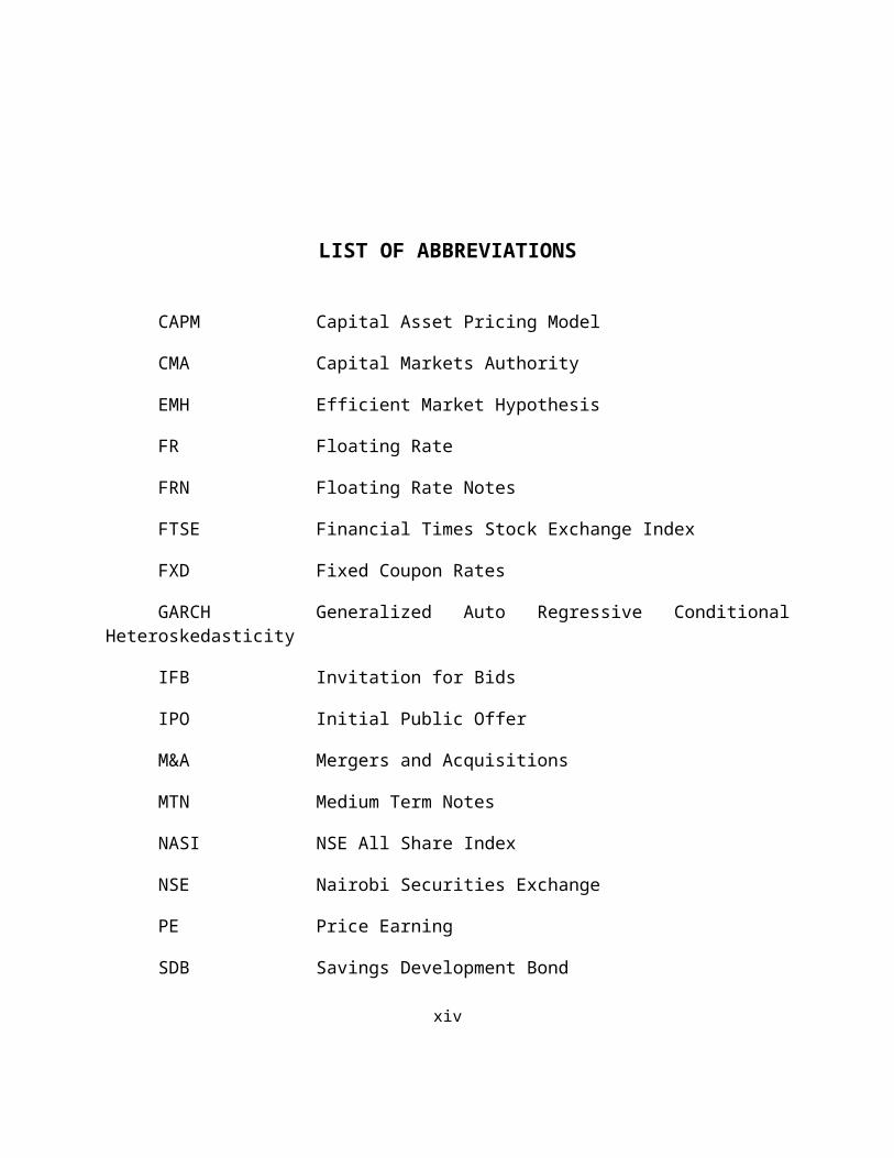
LIST OF ABBREVIATIONS

CAPM Capital Asset Pricing Model

CMA Capital Markets Authority

EMH Efficient Market Hypothesis

FR Floating Rate

FRN Floating Rate Notes

FTSE Financial Times Stock Exchange Index

FXD Fixed Coupon Rates

GARCH Generalized Auto Regressive ConditionalHeteroskedasticity 

IFB Invitation for Bids

IPO Initial Public Offer

M&A Mergers and Acquisitions

MTN Medium Term Notes

NASI NSE All Share Index

NSE Nairobi Securities Exchange

PE Price Earning

SDB Savings Development Bond

xiv

TURDEX Turkish Derivatives Exchange

xv

CHAPTER ONE

INTRODUCTION

1.1 Background of the Study

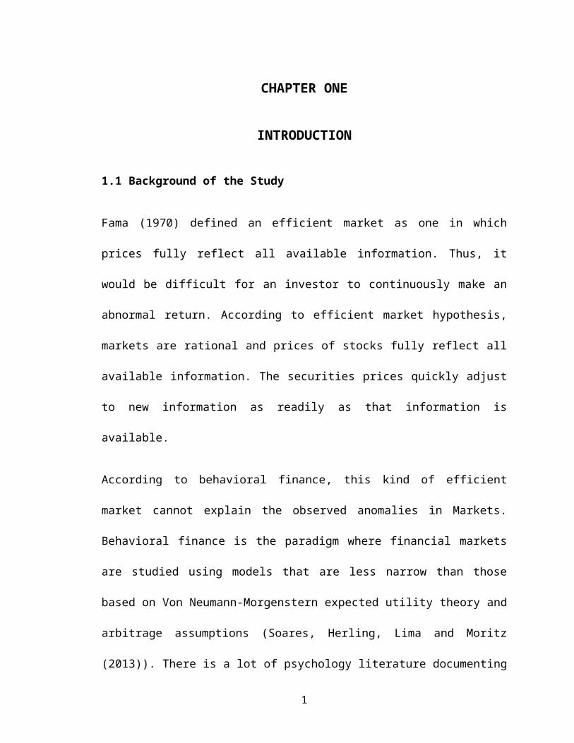
Fama (1970) defined an efficient market as one in which

prices fully reflect all available information. Thus, it

would be difficult for an investor to continuously make an

abnormal return. According to efficient market hypothesis,

markets are rational and prices of stocks fully reflect all

available information. The securities prices quickly adjust

to new information as readily as that information is

available.

According to behavioral finance, this kind of efficient

market cannot explain the observed anomalies in Markets.

Behavioral finance is the paradigm where financial markets

are studied using models that are less narrow than those

based on Von Neumann-Morgenstern expected utility theory and

arbitrage assumptions (Soares, Herling, Lima and Moritz

(2013)). There is a lot of psychology literature documenting

1

that people make systematic errors in the way that they

think: they are overconfident, they put too much weight on

recent experience, etc. Their preferences may also create

distortions. Behavioral finance uses this body of knowledge,

rather than assuming that it should be ignored. Limits to

arbitrage refer to predicting in what circumstances

arbitrage forces are effective, and when they won't be.

Behavioral finance uses models in which some agents are not

fully rational, either because of preferences or because of

mistaken beliefs.

Anomalies have been discovered which contradict the

efficient market hypothesis. One of the anomalies is the day

of the week effect. Research findings have documented that

stock returns are high on Fridays and low on Mondays

(Nyamosi (2011)). This anomaly is however not explained by

any of the assets pricing models like the Capital Asset

Pricing Model. Patell and Wolfson (1984) observed that

prices adjust fast when new information becomes available.

They found that, when a firm publishes its latest earnings

2

or announces a dividend change, the major part of the

adjustment in the price occurs within five to ten minutes of

the announcement.

Studies by Kendall (1953) and Fama (1965) on testing weak

form efficiency carried out on the developed market,

generally agree with the weak-form efficiency of the market

considering a low degree of serial correlation and

transaction cost. The studies supported the proposition that

price changes are random and past changes are not useful in

forecasting future price changes particularly after

transaction costs are taken into account.

1.1.1 Day of the Week Effect

Poshakwale (1996) defined day of the week effect as the

existence of a pattern on the part of stock returns, whereby

these returns are linked to a particular day of the week. He

noted that such a relationship has been verified mainly in

USA, where the last trading days of the week, particularly

Friday are characterized by positive and substantial returns

while Monday the first trading day differs from the other

3

days by producing negative returns. Cross (1973) noted that

the presence of such an effect would mean that equity

returns are not independent of the day of the week which is

evidence against random walk theory.

Following the seminal paper of Fields (1931), various

studies have confirmed the day of the week effect, where

returns are significantly higher on some days of the week.

According to Bailey, Alexander and Sharpe (1999), seasonal

patterns in stock returns should be quite minor (if they

exist at all), because they are not suggested by traditional

asset pricing models. It is often assumed that the expected

daily returns on securities are the same for all the days of

the week. That is, the expected return on a given stock is

the same for Monday as it is for Tuesday as it is for

Wednesday as it is for Thursday and as it is for Friday.

Cabello and Ortiz (2002) demonstrated that there are

differences in distributions of stock returns in each of the

days-of-the-week. Accordingly, the average return on Monday

4

is significantly less than the average return during the

other days-of-the-week. Whereas, according to the Efficient

Market Hypothesis (EMH), the expected daily returns on

stocks are the same for all days-of-the week. The study by

Gibbon and Hess (1981) established that the daily seasonal

effect is strong and that there are persistent negative mean

returns for stocks and below average returns for bills on

Mondays.

1.1.2 Bonds Returns

Jordan and Fischer (2002) defined return as the motivating

force and the principal reward in the investment process and

it is the key method available to investors in comparing

alternative investments. They document that return has two

components. The basic component is the periodic cash

receipts (or income) on investments, either in the form of

interest or dividends. The second component is the change in

the price of the asset – commonly called capital gain or

loss. This element of return is the difference between the

purchase price and the price at which the asset can be sold.

5

According to Reilly and Brown (2003) on the other hand,

return is the compensation for the time, the expected rate

of inflation and the uncertainty of the return after

investing in stocks. Shiller (2003) indicated that the stock

market is “macro efficient but micro inefficient” since

there is considerable predictable variation across firms in

their predictable future dividend of interest repayments but

little predictable variation in aggregate dividends or

interest. Therefore, changes in securities returns among

individual securities makes more sense than movement in the

market as a whole.

Fama and French (1993) show that default and term premium

are priced factors in the corporate bond market. Gebhardt,

Hvidkjaer, and Swaminathan (2005) show that default betas

are significantly related to the cross-sectional variation

of average bond returns. Furthermore, yield-to-maturity

remains the only significant characteristic after

controlling for default and term betas, suggesting that

systematic risk factors are important for pricing corporate

6

bonds. Lin, Wang, and Wu (2011) argue that market-wide

liquidity risk is also a factor in the cross-section of

corporate bonds as implied by their finding of a positive

and significant relation between average bond returns and

liquidity beta which is robust to including default and term

betas. Acharya, Amihud, and Bharath (2013) also show that

time-varying liquidity risk matters for corporate bonds.

1.1.3 Day-of-the-Week Effect and Bonds Returns

The day of the week effect is a phenomenon that develops a

form of anomaly of the efficient market theory. According to

Soares et al. (2013), this phenomenon explains that average

daily returns vary at different days but the same can be

considered under the efficient market theory. It is very

important for an investor to understand the working of

capital markets. The relationship between information and

bond prices is explained by the market efficiency. By the

day of week effect, the investor will consider the mean of

return for different days. In a decision making process, a

rational financial decision maker must take into account not

7

only returns but also the variance and volatility of

returns. It is very important to identify the return and

also the relationship between the returns (Hussain, Hamid,

Akash and Khan (2011)).

Bailey, Alexander and Sharpe (1999), observed that seasonal

patterns in securities returns should be quite minor because

they are not suggested by traditional asset pricing models.

It is often assumed that the expected daily returns on

securities are the same for all the days of the week. That

is, the expected return on a given security is the same for

Monday as it is for Tuesday as it is for Wednesday as it is

for Thursday and as it is for Friday. The fact that these

effects exist for such a long period of time is itself an

anomaly as according to efficient market hypothesis all

these effects should disappear once they are studied by

researchers and explained to the traders.

However, studies by Polwitoon and Tawatnuntachai (2008) show

that these anomalies still exits, while on the other hand

8

Arize and Nippani (2007) show that on the developed markets

some of these effects are disappearing or losing power.

Johnston, Kracaw and McConnell (1991) provide a

comprehensive study of weekly seasonal effects in T-bond, T-

note, and T-bill futures returns. Two distinct patterns are

found in returns on T-bond and T-note contracts, while no

day of the week effect is noted for T-bill futures. A

negative Monday effect is found for T-bond contracts. A

positive Tuesday effect is found on T-bond and T-note

contracts. The evidence indicates that the significance of

day of the week effect depends in an important way on the

time period studied. The negative Monday effect occurs only

in the data before 1982, while the positive Tuesday effect

is present only after 1984. In addition, we find that both

seasonal phenomena occur only during months prior to a

delivery month. This effect appears to be related to the

calendar month. More specifically, the Monday effect is

apparently concentrated during February, while the Tuesday

effect is concentrated during May.

9

1.1.4 Nairobi Securities Exchange

The Nairobi Securities Exchange (NSE Handbook (2010)) was

constituted as Nairobi Stock Exchange in 1954 as a voluntary

association of stockbrokers in the European community

registered under the Societies Act. It provides services for

stock brokers and traders to trade stocks, bonds, and other

securities. The Securities Exchange provides companies with

the facility to raise capital for expansion through selling

shares and securities to the investing public. The NSE plays

an important role in the economy of bringing the borrowers

and lenders of money together at a low cost. The typical

ownership identities at the NSE are by the government,

foreigners, institutions, individual and diverse ownership

forms.

The FTSE NSE Kenyan Shilling Government Bond Index is

designed to measure the average performance of eligible

government bonds with differing maturity bands. The

underlying constituents are based on Kenyan Government

Securities quoted on the NSE with maturity levels of more

10

than one year and notional amounts above KES5 billion. The

bonds market in Kenya involves both the treasury and

corporate bonds. Treasury bonds were introduced as early as

mid-1980s while corporate bonds came into the market in 1996

during the reform period. Despite the early initiation of

treasury bonds in the market, the market remained almost

stagnant, with the government using treasury bills to

finance domestic debt. It was not until 2001 when the

government took a deliberate effort to develop the market

that activities of the treasury bonds market increased

(Mbewa, Ngugi & Kithinji (2007)). The Corporate bonds traded

at the NSE as at 31st December 2013 are issued by 11

companies which trade both in stocks and bonds (Appendix 1).

1.2 Motivation for the Study

While there have been many studies on equity market, much

less effort has been dedicated to examination anomalies on

the fixed-income side in the Kenyan securities market. A

comparison of trading volumes of the financial markets

indicates that bonds are vital for every financial system. A

11

study of bonds price behavior will give the opportunity to

compare return patterns of bonds and therefore help in

finding the causes and explanation of this phenomenon.

1.3 Research Problem

The movement of stock market prices is an important

determinant of returns. Investors are not guaranteed of

“good” returns simply because the firm’s earning power has

grown. Rather, the time (day, week or month) can also

determine the investors return. The day of the week effect,

one of the documented anomalies, has revealed that security

returns tend to be significantly higher in some days of the

week relatively to other days of the week (Gerald, Vivek &

Ninon 2006).The predictability of stock return is a feature

of inefficient stock market.

While various research studies have been undertaken on the

day of the week effect on stocks at the NSE, the same has

not been done on bonds. By comparing the findings with the

earlier studies it was therefore possible to compare the

12

findings and thus draw conclusions based on both stocks and

bonds returns. According to Mykhailo (2009), the empirical

analysis for the bond markets show clear signs of Tuesday

effect for most countries. This fact was confirmed by

regression on dummies and bootstrap analysis. At the same

time, stock markets show no evidence for any day-of-the-week-

effect as a result of application of mentioned methods.

Mokua (2003), in his study on the weekend effect on the

stocks at the NSE concluded that weekend effect does not

exist in Nairobi Securities Exchange. Makokha (2012) results

obtained show that Tuesday has the highest positive return

and Wednesday has the highest negative return. Stock return

volatility is highest on Tuesday and lowest on Friday. The

study concludes that there is no day of the week effect at

the Nairobi Securities Exchange. Muthama and Mutothya (2013)

suggest that a random walk model cannot be a good

description of successive price returns at the Nairobi stock

exchange. This implies that there are anomalies in existence

at the NSE and thus it would be possible to take advantage

13

of differing stocks returns in the securities market. Kulavi

(2013) indicates that there is existence of day of the week

effect in the Nairobi Securities Exchange and the highest

volatility is experienced on Monday and lowest volatility is

experienced on Thursday.

In the studies by Kulavi (2013), Makokha (2012), Muthama and

Mutothya(2013) the findings were based on trading in equity

and therefore it is inconclusive if the same would apply in

the trading of bonds at the NSE. These findings therefore

lead to the research problem: Does the day of the week effect exist at

the NSE and what is its effect on bonds trading returns?

1.4 Objective of the Study

To determine the relationship between of day of the week and

bonds trading returns at the Nairobi Securities Exchange.

14

1.5 Value of the Study

1.5.1 Academicians

The study is aimed at filling the existing knowledge gap.

The study will also benefit the students as a basis of

reference for any future study in the field of market

efficiency. Thus to academicians who want to contribute to

the body of knowledge, this research will help in opening up

opportunities for doing further research.

1.5.2 Investors

The study will benefit the investor in the sense that,

information gathered on day of the week trends will enable

them to take advantage of the regular shifts in the market.

The investor was in a position to take advantage of

different rates of return during different days of the week

while trading in bonds in the stock market.

1.5.3 Securities Market Regulators

The study will enable monitoring of the activities of the

securities market with respect to the changes in the day of

15

the week hence was able to measure the performance of the

stock market which is a signal of economic stability in the

country.

1.5.4 Securities Brokers and Dealers

The knowledge of such crucial information on day of the week

and may assist the stock brokers to plan well when to trade.

It will also enable them to know how to get supernormal

returns that is by buying the securities on the day of the

week when prices are low and selling them on the day when

prices are high. It will enable them to maximize on their

returns.

16

CHAPTER TWO

LITERATURE REVIEW

2.1 Introduction

This chapter includes an analysis of the Efficient Market

Hypothesis as an explanation of different returns in

different securities markets. It then explains behavioural

finance as a factor in explaining why markets experience

irrational influences. The study will then explain the

determinants of bonds returns. It continues by focusing on

the empirical studies which have been carried out in the

recent past. One of the anomalies that has been extensively

discussed in this chapter is the day of the week effect in

relation to bond returns. The chapter ends by summarizing

what has already been established in previous research

studies and thus the research gap which this study seeks to

fill.

17

2.2. Efficient Market Hypothesis

According to Fama, Fisher, Jensen and Roll (1969) EMH is an

investment theory which states that it is impossible to

“beat the market” because stock market efficiency causes

existing securities prices to always incorporate and reflect

all the relevant information. According to the EMH, this

means that stocks trade at their fair value and thus it is

impossible for investors to either purchase undervalued

stocks or sell stocks for inflated prices.

Fama (1970) divided market efficiency into three categories,

these are: Weak form, Semi-strong form and Strong form of

market efficiency. The strong form suggests that securities

prices reflect all available information including private

information. This means that even corporate insiders cannot

make abnormal profits by using inside information. The semi-

strong form of EMH asserts that securities prices reflect

both past and present information i.e. all publicly

available information. The weak form of the EMH states that

it is impossible to predict future stock prices by analyzing

18

prices from the past. The current price is a fair one that

considers any information contained in the past price data

and therefore charting techniques are of no use in

predicting stock prices.

The EMH has provided the theoretical basis for much of the

financial market research during the seventies and the

eighties. In the past, most of the evidence seems to have

been consistent with the EMH (Seyhun (1986)). Prices were

seen to follow a random walk model and the predictable

variations in equity returns, if any, were found to be

statistically insignificant. While most of the studies in

the seventies focused on predicting prices from past prices

(Malkiel (1977)).

2.3 Behavioral Finance Theory

Behavioral finance seeks to supplement the standard theories

of finance by introducing behavioral aspects to the decision

making process (Ndungu, (2012)). Behavioral finance deals

with individuals and how they gather and use information. It

19

seeks to understand and predict systematic financial market

implications of psychological decision processes. In

addition, it focuses on the application of psychological and

economic principles for the improvement of financial

decision making (Olsen, (1998)). Market efficiency, in the

sense that market prices reflect fundamental market

characteristics and that excess returns on the average are

leveled out in the long run, has been challenged by

behavioral finance. Some market anomalies cannot be

explained with the help of standard financial theory, such

as abnormal price movements in connection with IPOs, M&A,

stock splits and spin-offs.

In the recent past, statistical anomalies have continued to

appear which suggests that the existing standard finance

models are probably incomplete. Investors have been shown

not to react “logically” to new information but to be

overconfident and to alter their choices when given

superficial changes in the presentation of investment

information (Olsen (1998)). During the past few

20

years there has, for example, been a media interest in

technology securities. Most of the time there has been a

positive bias in assessments especially in the media which

might lead investors in making incorrect investment

decisions. These anomalies suggest that the underlying

principles of rational behavior underlying the efficient

market hypothesis are not entirely correct and that there is

need to look, as well, at other models of human behavior as

have been studied in other social sciences (Shiller (1998)).

2.4 Determinants of Bonds Returns

2.4.1 Issue Size

Size should have a significant positive impact on bond

liquidity, as dealers can more easily manage their inventory

of larger issues. While studies using yield spreads to proxy

for liquidity find little support for this hypothesis, Hong

and Warga (2000) show that larger issues have significantly

tighter bid-ask spreads. Alexander, Edwards, and Ferri

21

(2000) find that larger issues do have higher trading

volume, thus attracting a higher return on the bonds.

2.4.2 Age of Bonds

Alexander, Edwards, and Ferri (2000) and Warga (1992) argue

that as a bond becomes more seasoned it becomes less liquid,

as inactive portfolios absorb progressively more of the

original issue and less is available to trade. Prior

evidence shows that yield spreads increase as the bond ages

(Sarig and Warga (1989), Warga (1992)), bid-ask spreads

increase (Chakravarty and Sarkar (2003), Hong and Warga

(2000), Schultz (2001)), and trading volume decreases

(Alexander, Edwards, and Ferri (2000)).

2.4.3 Interest Rate Risk

Alexander, Edwards, and Ferri (2000) show that bonds with

higher interest-rate risk have a stronger speculative

trading component. The theoretical literature (Harris and

Raviv (1993), Kandel and Pearson (1995)) suggests that

22

differences in investors' forecasts should lead to more

speculative trading in the highest duration issues.

2.4.4 Credit Risk

Uncertainty concerning value is likely to be higher for

lower credit quality issues. Speculation about changes in

the bond's credit quality, which are more likely for lower

grade bonds, should induce more trading. Hotchkiss and Ronen

(2002) show that lower grade bonds are more likely to

reflect firm specific information. Alexander, Edwards, and

Ferri (2000) document more trading in high-yield bonds with

higher credit risk.

2.4.5 Equity Trading Volume and Return

Firm-specific news should affect trading in both the equity

and debt of a firm. Based on high-yield bond data from,

Hotchkiss and Ronen (2002) find support for the hypothesis

that bond and stock returns react jointly to common factors.

In contrast, Kwan (1996) finds that only past stock returns

are correlated with current bond yield changes. For bonds of

23

companies with publicly traded equity, we expect stock

activity and bond liquidity to be positively related.

2.4.6 Equity Market Conditions

Financial market conditions influence bond trading as

investors optimize and rebalance their portfolios in light

of new information. The literature on the relationship

between market volatility and liquidity is divided. Gallant,

Rossi, and Tauchen (1992) observed a positive correlation

between market volatility and trading volume of NYSE-traded

stocks.

2.5 Empirical Review

2.5.1 Calendar Anomalies in Fixed Income Instruments

Cross (1973) in his study of calendar anomalies found out

that Monday had a negative return while Friday had a

positive return. He analyzed the Standard and Poors

composite index from 1953 to 1970. Cross, further indicated

that the performance on Monday was dependent on Friday’s

performance. French (1980) had results that were consistent

24

with those of Cross (1973). French studied the Standard and

Poors composite index from 1953 to 1977. He observed that

returns remained dependent on the day of the week. Further

tests revealed that Monday mean returns over the study

period were significantly negative while Wednesday through

Friday returns were significantly positive. On the other

hand Aggrawal and Tandon (1994) also found a day-of- the-

week effect in 18 equity markets.

Independent studies conducted by French(1980) and Gibbons

and Hess(1981) found evidence consistent with the hypothesis

that there are significant differences in the expected

percentage changes for stocks depending on the day of the

week. The study covered more than 4,000 trading days from

1962 through 1968. The expected percentage change on Mondays

appeared to be negative and the expected percentage change

on Wednesdays and Fridays appeared to be larger than on

Tuesdays and Thursdays.

Gibbons and Hess (1981) found evidence of a significant

negative Monday return in US Treasuries between 1962 and

25

1968. However, Jordan and Jordan (1991) conducted

seasonality tests for corporate bonds on the Dow Jones

composite bond average for the period 1963-1986. There was

no significant difference in mean daily returns for fixed

income securities. Kohers and Patel (1996), Adrangi and

Ghazanfari (1996) all detected various degrees of daily

seasonality. Oduncu (2012) examined the day of the week

effect on the Turkish Derivatives Exchange and his study

concluded that the day of the week effect is not present at

TURKDEX.

Mykhailo (2009) investigated the existence of calendar

effects on the bond market of selected emerging countries

and conducted comparative analysis of these effects on the

stock and bond markets. The empirical analysis for the bond

markets show clear signs of Tuesday effect for most

countries. This fact was confirmed by regression on dummies

and bootstrap analysis. At the same time, stock markets

showed no evidence for any day-of-the-week-effect as a

result of application of the mentioned methods. Day-of-the-

26

month effect, on the other hand, was found significant for

both stock and bond markets: returns for the end of the

month are higher than for the rest of the month. As it was

expected the size of this effect was bigger for the stock

market as equity is associated with higher risk.

Klesov (2008), researched on calendar effects for stock

markets of selected developing countries. According to his

work, intraweek effect (Friday effect) was found for most

countries with the usage of bootstrap approach, while Monday

effect was found only for a couple of countries using GARCH

approach. The evidence for day-of-the-week and month-of-the-

year was partly significant due to the relatively small size

if the dataset.

Polwitoon and Tawatnuntachai (2008), examined the behavior

of U.S.-based emerging market bond funds over a period from

1996 to 2005, the top six holding countries were Argentina,

Brazil, Mexico, Philippines, Russia and Venezuela (almost

all bonds are denominated in dollars). This paper analyzed

27

only month-of-the-year effect for the bond funds and found

positive effect in November and December. This is most

likely caused by common reason of end-of-the-year activity

bursts on the capital markets.

Marrett and Worthington (2011) examined month of the year

effect in the Australian daily market returns using a

regression-based approach. The results indicated that the

returns are significantly higher in April, July and December

combined with evidence of a small cap effect with

systematically higher returns in January, August, and

December. The analysis of the sub-market returns was also

supportive of disparate month of the year effects.

2.5.2 Calendar Anomalies at the Nairobi Securities Exchange

Muthama and Mutothya (2013) carried out an investigation on

whether stock prices at the NSE follow a random walk theory.

The study employed serial correlation tests and runs tests

to analyze daily price returns for eighteen companies whose

stocks constituted the NSE 20 share over the period July

2008 to June 2011. The findings suggest that random walk

28

model cannot be a good description of successive price

returns at the Nairobi stock exchange.

Makokha (2012) conducted an investigation in the Kenyan

stock market to test whether the day of the week anomaly

exists. Daily market capitalization was used to compute the

stock return and carry out multiple regression from January

2008 to December 2011. The results obtained show that

Tuesday has the highest positive return and Wednesday has

the highest negative return. Stock return volatility is

highest on Tuesday and lowest on Friday. The study concludes

that there is no day of the week effect at the Nairobi

Securities Exchange.

In testing the existence of January effect at the NSE,

Nyamosi (2011) carried out a descriptive research. The

population of interest in the study consisted of fifty two

firms listed for equity stocks at the NSE for the period

2001 to 2010. Their mean returns were used to investigate

the existence of January effect at the NSE. The data

29

comprised of the monthly share prices and returns.

Regression analysis of beta co-efficients of the model

showed negative co-efficients between the average dependent

variable for the months of February through December and an

average positive dependent variable for January. This

confirmed higher returns in January compared to the other

months.

Onyuma (2009) in determining the existence of daily and

monthly seasonal anomalies in the NSE used stock returns in

his study. He used regression analysis in analyzing the Data

on prices and adjusted returns derived from the NSE 20 index.

The study covered a period of twenty six years from 1980 to

2006. It confirmed that both the daily and monthly seasonal

anomalies do exist in the NSE.

2.6 Conclusion

This chapter has reviewed the various studies on day of the

week effect in different markets in the world involving both

30

stocks and bonds. The findings have different conclusions

based on the location of the market and the timing of the

study. There have been different explanations for this day of

the week anomaly. Some researchers have attributed the anomaly

to new negative information originating from the long weekend.

Other researchers have not been able to provide any

information. The findings of this research hopefully will add

to the available literature on day of the week effect in the

Kenyan bond market.

31

CHAPTER THREE

RESEARCH METHODOLOGY

3.1 Introduction

This chapter gives a description of the research methodology

employed in achieving the objectives of this study. The

chapter presents the research design, target population and

sampling procedure, data collection procedures, and data

analysis.

3.2 Research Design

Research design constitutes the basis for collection,

measurement and analysis of data. The study took the form of

a descriptive research design. Kombo and Tromp (2006) stated

that descriptive studies are not only restricted to fact

findings, but may often result in the formulation of important

principles of knowledge and solution to significant problems.

The design served a variety of research objectives such as

descriptions of the characteristics associated with the

32

subject population, estimates of proportions of a population

that have these characteristics and discovery of associations

among different variables. It involved measurement,

classification, analysis, comparison and interpretation of

daily bond prices from the NSE statistically to determine the

relationship between the day of the week and bond prices at

the NSE. The descriptive research design enabled an easy

analysis of the huge data obtained from the NSE by reducing

the ambiguity of the research evidence and ensured that the

evidence answered the research question unambiguously.

3.3 Population

The population of interest for this research was composed of

all the 11 listed companies that have issued bonds at the

Nairobi Securities Exchange. The data from all the 11

companies was used based on availability and access.

3.4 Data Collection

The data for this study was collected from the NSE.

Secondary data for the daily market capitalization from

January 2009 to December 2013 (5 Years) was used. The data

33

series comprised of the daily market index, daily prices of

the 11 firms which have issued bonds at the NSE.

3.5 Data Analysis

To meet the objective, the data was analysed and tested to

yield conclusions on the existence of Day of the Week Effect

on bond returns at the NSE. The study adopted the regression

model used by Makokha (2012). The period of the study was

from January 2nd, 2009 to December 31st 2013. The daily bond

prices for each company were used to compute daily returns,

Rt.

Rt = ln (Ct / Ct-1) × 100%

Where:

ln is the natural logarithm operator,

C is the daily price for each individual bond.

Daily returns computed this way were then continuously,

compounded, and percentage returns from day to day

calculated. Initially, the research employed dummy variable

34

regression to determine the day-of-the-week effect at the

NSE. A linear regression was run where each day is

represented by a dummy variable equal to one if the return

is for the day and equal to zero if the return is for

another day.

Rd = DMRM + DTRT + DWRW + DRRR + DFRF + εt

Where:

Rd is the bond return,

DM, DT, DW, DR, DF represent the dummy variables for Monday,

Tuesday, Wednesday, Thursday, and Friday respectively

RM, RT, RW, RR, RF represent the return for Monday, Tuesday,

Wednesday, Thursday, and Friday respectively

εt is an error term

This model assumed that the error terms and variances are

constant across time. In addition, Wooldridge (2003) shows

that multiple linear regression assumes that the parameters

are linear, the sample is random, the error terms are mean

35

zero, none of the variables are perfectly collinear, and the

regression coefficients are unbiased.

The research used five dummy variables as independent

variables and the bonds return as a dependent variable. The

t-test was used to test if there is a significant difference

in bonds returns across the five days of the week. The

research also used the F-test to test the extent to which

the deviations of these daily bond returns are different.

Most past research works on daily market anomalies have used

the method of regression using dummy variables. This is the

reason why this research adopted the same methodology. This

made it easy to compare the results with the earlier

findings.

36

CHAPTER FOUR

DATA ANALYSIS, RESULTS AND DISCUSSION

4.1 Introduction

This chapter focuses on the results of data analysis and

discussion of findings. The aim was to document the day of

the week effect on bond returns. The data was collected from

the 11 companies that had issued corporate bonds and covered

the period 2009 – 2013. The study used both descriptive and

inferential statistics to analyze the data found. It

addresses issues such as the: descriptive statistics;

regression results; and correlation coefficients among the

variables. Data analysis results were presented using

tables.

4.2 Descriptive Statistics

This sub-section gives the summary statistics of the main

variables that have been included in the model including:

37

minimum, maximum, mean, standard deviation, skewness,

kurtosis and tests for normality.

Table 4.1: Descriptive Statistics

Monday Tuesday

Wednesday

Thursday

Friday

BondReturn

N 52 52 52 52 52 52Mean 0.0129 0.0130 0.0049 0.0020 0.007

2

0.005

7Std. Deviation 0.1184 0.1239 0.1003 0.0927 0.009

4

0.065

0Skewness 0.645 0.675 0.803 0.867 1.144 0.644Std. Error of

Skewness

0.33 0.33 0.33 0.33 0.33 0.33

Kurtosis 1.894 1.487 2.425 3.065 3.023 1.936Std. Error of

Kurtosis

0.65 0.65 0.65 0.65 0.65 0.65

Minimum -

0.3040

-

0.2983

-0.2158 -

0.2211

-

0.012

0

-

0.163

0Maximum 0.3732 0.3918 0.3458 0.3207 0.040

1

0.192

91st Quartile -

0.0490

-

0.0621

-0.0366 -

0.0338

0.002

5

-

0.026

32nd Quartile - - -0.0088 - 0.005 0.000

38

0.0039 0.0084 0.0055 4 73rd Quartile 0.0827 0.0864 0.0364 0.0254 0.009

7

0.028

3

The results showed that the Monday bond return had a mean of

0.0129 with a minimum of -0.304, a maximum of 0.3732,

skewness 0.645 and kurtosis of 1.894. Tuesday bond return

had a mean of 0.0130, minimum of -0.2983, maximum of 0.3918,

skewness of 0.675 and kurtosis of 1.487. Wednesday bond

return had a mean of 0.0049, minimum of -0.2158, maximum of

0.3458, skewness of 0.803 and kurtosis of 2.425. Thursday

bond return had a mean of 0.0020, minimum of -0.2211,

maximum of 0.3207, skewness of 0.867 and kurtosis of 3.065.

Friday bond return had a mean of 0.0072, minimum of -0.0120,

maximum of 0.0401, skewness of 1.144 and kurtosis of 3.023.

Overall bond return had a mean of 0.0057, minimum of -

0.1630, maximum of 0.1929, skewness of 0.644 and kurtosis of

1.936.

Analysis of skewness shows that Monday, Tuesday, Wednesday

and Thursday are asymmetrical to the right around its mean.

39

Additionally, Thursday and Friday is highly peaked compared

to other regressors.

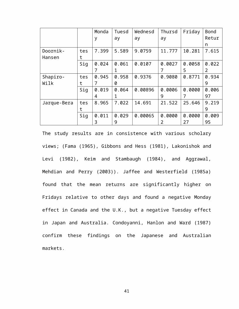
4.3 Normality Test

Jarque-Bera, Doornik-Hansen and Shapiro-Wilk tests are test

statistics for testing whether series are normally

distributed. They measure the difference of the skewness and

kurtosis of the series with those from the normal

distribution using the null hypothesis of a normal

distribution. They hypothesize that:

H0: Sample follows a Normal distribution.

Ha: Sample does not follow a Normal distribution.

When the p-value is greater than the alpha value (α ≤ .05),

then one fails to reject the null hypothesis and don’t

accept the alternative hypothesis. From the results, the

null hypothesis of normal distribution is rejected as the

computed p-value is less than the significance level

alpha=0.05.

Table 4.2: Normality Test

40

Monday

Tuesday

Wednesday

Thursday

Friday BondReturn

Doornik-Hansen

test

7.399 5.589 9.0759 11.777 10.281 7.615

Sig 0.0247

0.0611

0.0107 0.00277

0.00585

0.0222

Shapiro-Wilk

test

0.9457

0.9580

0.9376 0.9080 0.8771 0.9349

Sig 0.0194

0.0641

0.00896 0.00069

0.00007

0.00697

Jarque-Bera test

8.965 7.022 14.691 21.522 25.646 9.2199

Sig 0.0113

0.0299

0.00065 0.00002

0.000027

0.00995

The study results are in consistence with various scholary

views; (Fama (1965), Gibbons and Hess (1981), Lakonishok and

Levi (1982), Keim and Stambaugh (1984), and Aggrawal,

Mehdian and Perry (2003)). Jaffee and Westerfield (1985a)

found that the mean returns are significantly higher on

Fridays relative to other days and found a negative Monday

effect in Canada and the U.K., but a negative Tuesday effect

in Japan and Australia. Condoyanni, Hanlon and Ward (1987)

confirm these findings on the Japanese and Australian

markets.

41

Kato and Schallheim (1985) also found that the Tuesday

return is negative and Wednesday and Saturday returns are

strongly positive in Japan. Jaffe and Westerfield (1989)

wrote a significant paper providing international evidence.

Bad-Friday effect, which refers to a decline of the market

on Fridays, usually precedes Monday with increased stock

selling pressure.

4.3.1 Multicollinearity – Correlation Matrix

Correlation matrix indicates a linear association of the

explanatory variables and helped in determining the

strengths of association in the model, that is, which

variable best explained the relationship between day of the

week and bond returns. It also helped in deciding which

variable(s) to drop from the equation. This helped test the

hypothesis:

H0: there is no significant relationship between day of the

week and bond returns

42

Ha: there is a significant relationship between day of the

week and bond returns

Table 4.3: Correlation Matrix

Day BondReturn

Monday Tuesday

Wednesday

Thursday

Monday PearsonCorrelation

.968**

1

Sig. (2-tailed)

.000

Tuesday PearsonCorrelation

.973**

.989 1

Sig. (2-tailed)

.000 .121

Wednesday

PearsonCorrelation

.866**

.872 .893 1

Sig. (2-tailed)

.000 .091 .070

Thursday

PearsonCorrelation

.399 .009 .006 -.216 1

Sig. (2-tailed)

.158 .948 .969 .124

Friday PearsonCorrelation

.490 .015 .007 -.101 .308

Sig. (2-tailed)

.527 .915 .962 .478 .096

From the Table 4.3, it can be deduced that there was a

positive correlation between bond returns and day of the

week. The first three days of the week exhibited strong,

positive and significant linear relationship with bond

43

returns: Monday (R = .968; p < .001), Tuesday (R = .973; p <

.001), and Wednesday (R = .866; p < .001). Thursday (R =

.399; p = .158) and Friday (R = .490; p = .527) had positive

but insignificant relationship with bond returns.

However, the independent variables had low collinearity

owing to their correlation value between them. According to

Babak (2012), the limitation of Pearson correlation

coefficient is that though it indicates the strength of a

linear relationship between two variables, its value

generally does not completely characterize their

relationship, thus, the subsequent analysis.

Table 4.4: Multicollinearity Test

Tolerance VIF

Monday .320 3.121

Tuesday .317 3.157

Wednesday .148 6.742

Thursday .718 1.394

Friday .894 1.118

44

Variance Inflation Factors (VIF) shows that there is low

collinearity amongst the independent variables as the VIF

values were below the critical value of 10: Monday (3.121),

Tuesday (3.157), Wednesday (6.742), Thursday (1.394), and

Friday (1.118). Besides, tolerance values were above the

critical values of 0.1. As stated by Studenmund (2006), the

variance (the square of the estimate's standard deviation)

of an estimated regression coefficient is increased because

of collinearity.

4.4 Regression Analysis

The regression method used for this study was the least

square method. This was used to determine the line of best

fit for the model through minimizing the sum of squares of

the distances from the points to the line of best fit.

Through this method, the analysis assumed linearity between

the dependent variable and the independent variables.

Table 4.5: Model Summary

R RSquare

Adjusted RSquare

Std. Error ofthe Estimate

Durbin-Watson

45

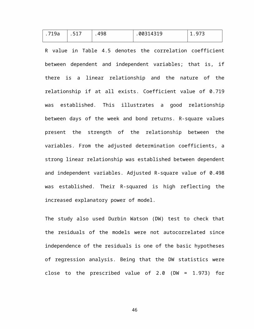
.719a .517 .498 .00314319 1.973

R value in Table 4.5 denotes the correlation coefficient

between dependent and independent variables; that is, if

there is a linear relationship and the nature of the

relationship if at all exists. Coefficient value of 0.719

was established. This illustrates a good relationship

between days of the week and bond returns. R-square values

present the strength of the relationship between the

variables. From the adjusted determination coefficients, a

strong linear relationship was established between dependent

and independent variables. Adjusted R-square value of 0.498

was established. Their R-squared is high reflecting the

increased explanatory power of model.

The study also used Durbin Watson (DW) test to check that

the residuals of the models were not autocorrelated since

independence of the residuals is one of the basic hypotheses

of regression analysis. Being that the DW statistics were

close to the prescribed value of 2.0 (DW = 1.973) for

46

residual independence, it can be concluded that there was no

autocorrelation.

Table 4.6: Analysis of Variance

Sum ofSquares

df MeanSquare

F Sig.

Regression

.215 5 .043 4347.188

.000b

Residual .000 46 .000

Total .215 51

Analysis of Variance’s (ANOVA) f-test was used to make

simultaneous comparisons between two or more means; thus,

testing whether a significant relation exists between

variables (dependent and independent variables); thus,

helping in bringing out the significance of the regression

model. Table 4.6 presents f-value 4347.188 at p < .001. It

can be concluded that the regression model was significant.

Table 4.7: Model Coefficients

UnstandardizedCoefficients

StandardizedCoefficients

t Sig.

B Std. Error Beta(Constant)

-.002 .001 -4.10

.090

47

8Monday .197 .026 .359 7.58

1.000

Tuesday .186 .027 .354 6.762

.002

Wednesday

.190 .011 .293 16.643

.040

Thursday

.172 .006 .245 30.675

.000

Friday .248 .050 .036 4.999

.031

The established regression equation for year 2005:

Bond Return = -0.002 + 0.197*Monday + 0.186* Tuesday +

0.190*Wednesday + 0.172*Thursday + 0.248*Friday

p < .001

From the finding in the above table the study found that

holding Monday – Friday returns at zero, the overall bond

returns was -0.002. Holding other factors constant, the

study found that a unit increase in Monday returns will lead

to an increase in bond returns by 0.197 (p < .001), a unit

increase in Tuesday returns will lead to an increase in bond

returns by a factor of 0.186 (p = .002), a unit increase in

Wednesday returns will lead to 0.190 (p = .040) increase in

bond returns, a unit increase in Thursday returns will lead

48

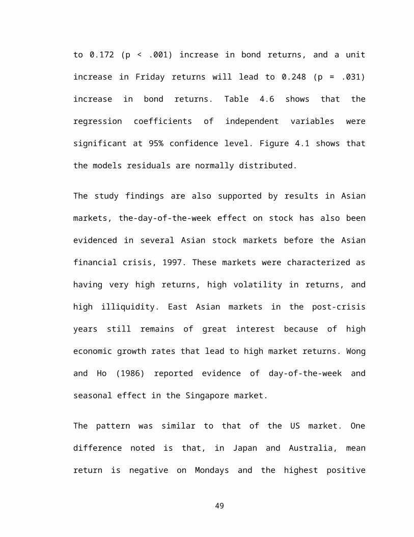
to 0.172 (p < .001) increase in bond returns, and a unit

increase in Friday returns will lead to 0.248 (p = .031)

increase in bond returns. Table 4.6 shows that the

regression coefficients of independent variables were

significant at 95% confidence level. Figure 4.1 shows that

the models residuals are normally distributed.

The study findings are also supported by results in Asian

markets, the-day-of-the-week effect on stock has also been

evidenced in several Asian stock markets before the Asian

financial crisis, 1997. These markets were characterized as

having very high returns, high volatility in returns, and

high illiquidity. East Asian markets in the post-crisis

years still remains of great interest because of high

economic growth rates that lead to high market returns. Wong

and Ho (1986) reported evidence of day-of-the-week and

seasonal effect in the Singapore market.

The pattern was similar to that of the US market. One

difference noted is that, in Japan and Australia, mean

return is negative on Mondays and the highest positive

49

return occurs on Fridays. The mean daily return in January

is higher than that for other months, although the end-of-

year effect is not significant at all. Aggarwal and Rivoli

(1989) noted day-of-the-week effect in Hong Kong, Korea,

Taiwan, Japan, and Singapore, while Ho’s (1990) paper finds

strong, seasonality effect – an evidence against the EMH -

in ten

Asia-Pacific markets, further confirming the day-of-the-week

effect in Singapore, Malaysia, Hong Kong, and Thailand.

Chen, Kwok, and Rui (2001) reported day of- the-week effect

in China, showing negative Tuesdays after 1995 and

highlighting that this anomaly disappears once non-normality

and spill-over from other countries is taken into account.

50

Figure 4.1: P-P Plot

4.5 Discussions

The results show that corporate bond returns follows day of

week signals. The market gave average positive returns on

all days. Friday, however, had the most returns given

positive returns in at least 75% of all the observations as

shown in the descriptive statistics.

Figure 4.2: Day of the Week Trend

Figure 4.3 shows that Monday, Tuesday and Wednesday returns

had the highest variability especially during mid-year and

towards the year end. In NSE, the maximum average return is

on Tuesday and had the highest standard deviation followed

51

by Monday. Thus, there is a signal of Tuesday effect.

However, Thursday exhibits near about zero return. This

implies that the average returns vary among the days of the

week. Hussain et al (2011) established a significant Tuesday

effect in Pakistani Stock market during a week exhibited by

high return unlike other days of the week which had constant

returns. Returns on Tuesday were more volatile over other days.

However, this is contrary to the Chukwuogor-Ndu (2006) findings that

occurrence of the highest daily return is evenly spread across

Thursday and Friday. The lowest return was experienced on Monday

and Wednesday.

The value of the skewness and kurtosis suggest that the return

distribution is not a normal distribution for all the days of the week.

Further the null hypothesis for the Jarque-Bera test of the presence of

normal distribution has been rejected at 1% level of significance. The

Efficient Market Hypothesis explains that there are constant market

returns for the whole week. The day-of-the-week effect happens

because perfect market do not exist. In economics, a perfect market is

defined by several condition. Among these conditions are: Perfect

market information, no participant with market power to set prices,

no intervention by governments, No barriers to entry or exit, equal

access to factors of production, profit maximization, and no

externalities. True perfect competition can exist only under a set of

conditions that are not possible in the real world, and so no real

52

perfect markets exist. The concept is used in economics, not to

describe any state of affairs in the real world, but as a construct to

simplify thought experiments about how economies work and provide

a benchmark to which real world markets can be compared.

53

CHAPTER FIVE

SUMMARY, CONCLUSION AND RECOMMENDATIONS

5.1 Introduction

This chapter presents discussions of the key findings

presented in chapter four, conclusions drawn based on such

findings and recommendations there-to. This chapter is

structured into summary, conclusions, recommendations and

areas for further research.

5.2 Summary

The objective of the study was to determine the daily bond returns for

the all five days of the week. It also sought to determine if there is a

significant difference in bond returns for all the five trading days. It

was then analysed using excel sheets and SPSS to compute the daily

stock market returns. From the analysis, Tuesday had the highest

return than any other day of the week. Wednesday on the other hand

had the lowest negative return. This contradicts the observation by

researchers such as Onyuma (2009) and many others who observed

that Monday had the lowest negative return while Friday had the

highest positive return.

54

5.3 Conclusion

Empirical results of this study indicate that there is a significant

Monday, Tuesday and Wednesday effect in bond market during a

week. On Friday there is high return. Returns on Mondays are more

volatile over other days. The results show that there is a significant

relationship between the dependent variable which is the bond market

return and independent variables which are the five days of the week.

The research findings indicate that there is little bond return volatility

at the NSE as judged by the distribution. Tuesday has the highest

volatility, then Monday, Wednesday and then Friday. The study

concludes that: the day of the week effect is present in mean returns

for the bond market return; there is strong evidence for the day of

the week effect in both return and volatility; and, it seems that bond

market anomaly exists in both return and volatility.

5.4 Recommendations

The day of the week effect patterns in return might enable investors

to take advantage of relatively regular market shifts by designing and

implementing trading strategies, which account for such predictable

patterns. The findings support that this potential advantage of

investors due to the day of the week effect anomaly is present in the

Kenya bond market.

55

5.5 Limitations of the Study

The corporate bond returns may have been affected by other

market and corporate event. Macroeconomic performance such

as inflation and environmental factors might also have

mediated the relationship between bond returns and day of

the week effect. These factors could not be isolated in the

study owing to difficulty in doing so.

5.6 Suggestions for Further Research

The study suggests that similar study can be conducted on stock

returns. This would produce a holistic view of the day of teh week

effect. This will allow for a comparison of the findings and

recommendations. Additionally, further studies can be conducted on

other periods such as January effect.

56

REFERENCES

Acharya, V., Amihud, Y., & Bharath S. (2013). Liquidity risk

of Corporate Bond Returns: Forthcoming, Journal of Financial

Economics.

Adrangi, B., & Ghazanfari, F. (1996). Corporate Bond Returns

and Weekday Seasonality, Journal of Applied Business Research,

13, 9–16.

57

Aggarwal, R. & Rivoli, P. (1989). Seasonal and Day of the

Week effects in Four Emerging Stock Markets, Financial

Review, 24, 541-50.

Aggarwal, R., Mehdian, S.M., & Perry, J.M. (2003). Day-of-

the-week Regularities and their Higher Moments in

Futures Markets. American Business Review 21, 47-53.

Agrawal, A., & Tandon, K. (1994). Anomalies or Illusions?

Evidence from Stock Markets In Eighteen countries,

Journal of International Money and Finance 13; 83 – 106.

Alexander, G., Edwards A., & Ferri, M. (2000). The

Determinants of the Trading Volume of High Yield

Corporate Bonds, Journal of Financial Markets, 3, 177-204.

Ariel, R.A. (1990). High stock returns before holidays:

existence and evidence on possible causes, Journal of

Finance, 45, 1611-1626.

Arize, A., & Nippani, S. (2007). U.S. Corporate Bond

Returns: A Study of Market Anomalies Based on Broad

58

Industry Groups, Review of financial economics 17 (2008) 157–

171

Babak, M.D. (2012). The Misleading Value of Measured

Correlation.

Bailey, J.V., Alexander G.J., & Sharpe W.F. (1999).

“Investments”, 6th Edn., Prentice Hall.

Ball, R. (1978). Anomalies in Relationships Between

Securities’ Yields and Yield- Surrogates, Journal of

Financial Economics, 6, 103-26.

Basu, S. (1977). Investment Performance of Common Stock in

Relation to their Price Earnings Ratio: A test of the

Efficient Market Hypothesis, Journal of Finance, 32, 663-

682

Brown, P., Keim, D., Kleidon, A., & Marsh, T. (1983). New

Evidence on the Nature of Size- Related Anomalies in

Stock Prices. Journal of Financial Economics, 12, 33-56.

Cabello, A., & Ortiz, E. (2002). Day of the Week and Month

of the Year Anomalies at the Mexican Stock Market.

59

Chakravarty, S., & Sarkar, A. (2003). A Comparison of

Trading Costs in the U.S. Corporate, Municipal and

Treasury Bond Markets, Journal of Fixed Income, 13(1), 39-

48.

Chen, G., Kwok, C.C.Y., & Rui, O.M. (2001). The Day-of-the-

Week Regularity in the Stock Markets of China. Journal of

Mathematical Financial Management, 11, 139-163.

Chukwuogor-Ndu, C. (2006). Stock Market Returns Analysis,

Day-of-the-Week Effect, Volatility of Returns: Evidence

from European Financial Markets 1997-2004. International

Research Journal of Finance and Economics, 1: 112-124.

Condoyanni, L., O’Hanlon J., & Ward, C.W.R. (1987). Day of

the week effects on stock returns: international

evidence. Journal of Business Finance and Accounting, 14, 159-

174.

Cross, F. (1973). The behaviour of stock prices on Friday

and Monday, Financial Analyst Journal 29, 67-60

60

Fama, E.F. (1965). The Behaviour of Stock Prices, Journal of

Business, 38, 34-105.

Fama, E.F. (1970), Reply to efficient capital market: A

review of theory and empirical work. Journal of Business

Finance, 25, 383-417.

Fama , E. F., Fisher, L., Jensen, M.C., and Roll, R. (1969).

The Adjustment of Stock Prices to the New Information,

International Economic Review, 10 (1), 1-21.

Fama, E.F., & French, K.R. (1993). Common Risk factors in

the Returns on Stocks and Bonds, Journal of Financial

Economics, 33, 3-56.

Fama, E.F., & French, K.R. (1995). Size and book –to- market

factors in earnings and returns, Journal of Finance, 50 ,

131-155.

Fields, M. J. (1931). Stock prices: a problem in

verification, Journal of Business, 7, 415-18.

French, K. (1980). Stock returns and the weekend effect.

Journal of financial Economics, 8, 55-69.

61

Gallant, R., Rossi, P., & Tauchen, G. (1992). Stock prices

and volume, Review of Financial Studies, 5, 199-242.

Gebhardt, W., Hvidkjaer, R., & Swaminathan, S. (2005). The

Cross-section of Expected Corporate Bond Returns:

Betas or Characteristics? Journal of Financial Economics 75,

84-114.

Gerald, K., Vivek, P., & Ninon, K. (2006). The Fading Day of

the Week in Developed Equity Market. Journal of Finance, 8,

12-18.

Gibbon, R., & Hess, P. (1981). Day of the week effects and

assets returns. Journal of Business, 54, 4, 579-596.

Harris, M., & Raviv A. (1993). Differences of Opinion Make

a Horse Race, Review of Financial Studies, 6, 473-506.

Ho, Y. K. (1990). Stock Returns Seasonalities in Asia

Pacific Market. Journal of International Financial Management and

Accounting 2, 44-77.

62

Hong, G., & A. Warga, A. (2000). An Empirical Study of

Corporate Bond Market Transactions, Financial Analysts

Journal, 56, 32-46.

Hotchkiss, E., & Ronen T. (2002). The Informational

Efficiency of the Corporate Bond Market: An Intraday

Analysis, Review of Financial Studies, 15(5), 1325-1354.

Hussain, F., Hamid, K., Akash, R.S., & Khan, M.I (2011). Day

of the Week Effect and Stock Returns: Evidence from

Karachi Stock Exchange-Pakistan. Far East Journal of Psychology

and Business, V 3, N 1.

Jaffe, R. and Westerfield (1985a). The weekend effect in

common stock returns: The International evidence.

Journal of finance, 40, 2, 433-454.

Jaffe, J., & Westerfield, R. (1989). The Weekend Effect in

common stock returns: The International evidence,

Journal of Finance, 46(2),529-554.

Johnston E.T., Kracaw W.A., & McConnell J.J. (1991). Day-of-

the-Week Effects in Financial Futures: An Analysis of

63

GNMA, T-Bond, T-Note, and T-Bill Contracts, Journal of

Financial and Quantitative Analysis v26 pp23-44.

Jordan, R., & Fischer, E.D. (2002). “Security Analysis and

Portfolio Management”, 6th Edition, Prentice Hall.

Jordan, S., & Jordan, B. (1991). “Seasonality in Daily Bond

Returns,” Journal of Financial and Quantitative Analysis, pp. 269-

285.

Kandel, E., & Pearson, N. (1995). Differential

Interpretation of Public Information and Trade in

Speculative Markets, Journal of Political Economy, 103, 831-

872.

Kato, K. & Schallheim, J.S., (1985). Seasonal and Size

Anomalies in the Japanese Stock Market. Journal of Financial

and Quantitative Analysis 20, 243–260.

Keim, D. & Stambaugh, R. (1984). Predicting Returns in the

Stock and Bond Market. Journal of Financial Economics,

17, 2, 357-390.

64

Kendall, M. G. (1953). The Analysis of Economic Time Series,

Part I: Prices. Journal of Royal Statistical Society, 96, 1, 11-

25.

Klesov, A. (2008). Calendar effects on stock market: Case of

selected CIS and CEE countries.

Kohers, T., & Patel, J. (1996). An Examination of the Day of

the Week Effect in Junk Bond Returns Over Business

Cycles, Review of Financial Economics, 5, 31–46.

Kombo, D.K., & Tromp, D.L.A. (2006). Proposal and thesis

writing: An introduction. Paulines Publicationa

Africa, 70-71.

Kulavi, C.M. (2013). Day of the Week Effect and Stock Market

Volatility: Evidence from Nairobi Securities Exchange

Kwan, S. (1996). Firm Specific Information and the

Correlation between Individual Stocks and Bonds, Journal

of Financial Economics, 40, 63-80.

Lakonishok, J., & Levi, M., 1982. Weekend effect in stock

return: A note. Journal of Finance 37, 883–889.

65

Lin, H., Wang, J., & Wu C. (2011). Liquidity Risk and

Expected Corporate Bond Returns. Journal of Financial

Economics 99, 628-650.

Lintner, J. (1965). The Valuation of Risk Assets and the

Selection of Risky Investments in Stock Portfolios and

Capital Budgets, Review of Economics and Statistics, 47, 13-37.

Makokha, A.S. (2012). Day of the Week Effect on Stock

Returns at the Nairobi Securities Exchange.

Malkiel, B.G. (1977). The Valuation of Closed Investment

Company Shares, Journal of Finance, 32,847-859.

Marrett, G., & Worthington, A. (2011). The month-of-the-year

effect in the Australian stock Market: A Short

Technical Note on the Market, Industry and Firm Size

Impacts, Australasian Accounting Business and Finance Journal, 5

(1), 117-123.

Mbewa, M., Ngugi, R., & Kithinji, A. (2007). Development of

Bonds Market: Kenya‘s Experience. Kenya Institute for Public

66

Policy Research and Analysis (KIPPRA) Working Paper No. 15,

December

Mbuthia, K.S. (2000). Calendar anomalies in the NSE.

Unpublished MBA Project, UON.

Mokua, M. (2003). Weekend effect on stock returns at the

NSE. Unpublished MBA Project, Uon.

Mossin, J. (1966) Equilibrium in Capital Asset Market,

Econometrica, 41, 867-87.

Muthama, N., & Mutothya, N. (2013). An Empirical

Investigation of the Random Walk Hypothesis of Stock

Prices at the Nairobi Stock Exchange, European Journal of

Accounting Auditing and Finance Research Vol.1, No.4, pp. 33-59.

Mykhailo, B. (2009). Calendar Effects in Daily Bonds

Returns: Case of Selected Emerging Economies.

NSE Handbook (2010).

Ndungu, D.I. (2012). Determinants of Individual Investor’s

Behavior in the Nairobi Securities Exchange.

67

Nyamosi, J.N. (2011). Testing the Effect of the January

Effect at the Nairobi Securities Exchange

Oduncu, A. (2012) “The Day of the Week Effect on the Turkish

Derivatives Exchange” European Journal of Economics, Finance

and Administrative Sciences ISSN 1450-2275 Issue 45 (2012)

Olsen, R. (1998). Behavioral finance and its implications

for stock price volatility. Association for Investment

Management and Research - Financial Analysts Journal, 54(2), 10-18.

Onyuma, S.O. (2009). Day of the week and month of the year

effect on the Kenyan stock market returns, East Africa

Social Science Research Review, 25, 2, 53-74.

Patell, J., and Wolfson, M. (1984). The Intraday Speed of

Adjustment of Stock Prices to Earnings and Dividend

Announcements, Journal of Financial Economics, 13, 223–252.

Polwitoon, S., and Tawatnuntachai, O. (2008). Emerging

Market Bond Funds: A Comprehensive Analysis, The

Financial Review 43 (2008) 51–84.

68

Poshakwale, S. (1996). Evidence on weak form efficiency and

day of the week effect in India Stock Exchange, Journal

of Finance, 3, 605-616.

Reilly, F., & Brown, K. (2003) Investment Analysis and

Portfolio Management, 7th Edition

Reinganum, M R. (1981) A New Empirical Perspective on the

CAPM, Journal of Financial and Quantitative Analysis, 16, 439-62.

Rozeff, M.S., & Kimney, W. R. (1976).Capital Market

Seasonality; The Case of Stock Returns, Journal of Financial

Economics, 3, 379-402.

Sarig, O., & Warga, A. (1989). Bond Price Data and Bond

Market Liquidity, Journal of Financial and Quantitative Analysis,

24, 367-378.

Seyhun, H.N. (1986). Insider Profits, Costs of Trading and

Market efficiency, Journal of Financial Economics, 16,189 -

212.

69

Sharpe, W. (1964) Capital Asset Prices: A Theory of Market

Equilibrium Under Conditions of Risk, Journal of Finance,

19, 425-42.

Shiller, R.J. (1998). Human Behaviour and the Efficiency of

the Financial System, Research Working Paper No. W6375.

Shiller, R. J. (2000). Irrational Exuberance. Princeton:

Princeton University Press.

Shiller, R. J. (2003). From Efficient Markets Theory to

Behavioral Finance, Cowles Foundation Paper No. 1055.

Schultz, P. (2001). Corporate Bond Trading Costs and

Practices: A Peek Behind the Curtain, Journal of Finance,

56, 677-698.

Soares, T., Herling L.H., Lima M.V., & Moritz G. (2013). Day

of the Week Effect and Stocks Returns: Evidence from

Ibovespa, Revista De Francas Aplicadas, 1-12.

Studenmund, A. (2006). Using Econometrics: A Practical

Guide. Boston: Pearson: Addison Wesley. 4, 245-273.

70

Warga, A. (1992). Bond Returns, Liquidity, and Missing Data,

Journal of Financial and Quantitative Analysis, 27 (4), 605-617.

Wong, K.A., & Ho, H.D (1986). The weekend effect on stock

returns in Singapore, Hong Kong Journal of Business

Management, 4: 31-50.

Wong, K.A., Hui, T.K., & Chan, C.Y. (1992). Day-of-the week

effects: Evidence from Developing Stock Markets. Applied

Financial Economics. 2, 49-56.

Wooldridge, J.M. (2003). Introductory Econometrics: A Modern

Approach, Thomson Southwestern, Mason, OH.

71

APPENDIX

Appendix 1: Corporate Bonds Traded at the NSE

Centum

Consolidated Bank of Kenya Ltd

Shelter Afrique

Barclays Bank

Mabati Rolling Mills

CFC Stanbic Bank

Kengen

I&M Bank

Housing Finance

Safaricom Ltd

PTA Bank Ltd

72

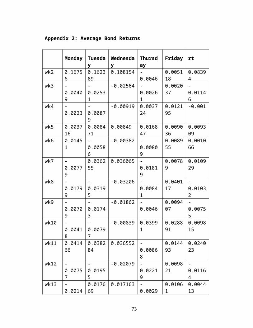
Appendix 2: Average Bond Returns

Monday Tuesday

Wednesday

Thursday

Friday rt

wk2 0.16756

0.162389

0.108154 -0.0046

0.005118

0.08394

wk3 -0.00409

-0.02531

-0.02564 -0.00261

0.002037

-0.01146

wk4 -0.0023

-0.00879

-0.00919 0.003724

0.012195

-0.001

wk5 0.003716

0.008471

0.00849 0.016847

0.009036

0.009309

wk6 0.01451

-0.00586

-0.00382 -0.00809

0.008955

0.001066

wk7 -0.00779

0.036255

0.036065 -0.01819

0.00789

0.010929

wk8 -0.01799

-0.03195

-0.03206 -0.00841

0.040117

-0.01032

wk9 -0.00709

-0.01743

-0.01862 -0.0046

0.009407

-0.00755

wk10 -0.00418

-0.00797

-0.00839 0.03991

0.028891

0.009815

wk11 0.041466

0.038284

0.036552 -0.00868

0.014493

0.024023

wk12 -0.00757

-0.01955

-0.02079 -0.02219

0.009821

-0.01164

wk13 -0.0214

0.017669

0.017163 -0.0029

0.01061

0.004413

73

5wk14 -

0.00182

-0.01096

-0.0117 -0.00214

0.006999

-0.00372

wk15 -0.00213

-0.00912

-0.00928 -0.06537

0.001738

-0.01607

wk16 -0.06575

-0.08046

-0.08019 0.092163

0.011275

-0.02553

wk17 0.093006

0.094392

0.093567 -0.0927

-0.01201

0.03102

wk18 -0.09395

-0.10425

-0.10309 0.12703

0.021701

-0.03233

wk19 0.126538

0.188735

0.189577 -0.05097

0.015293

0.086268

wk20 -0.05119

-0.06336

-0.06321 -0.06651

-0.01004

-0.04965

wk21 -0.06762

-0.08786

-0.08689 0.098905

0.015216

-0.0266

wk22 0.095558

0.097189

0.100477 -0.03191

-0.01166

0.045168

wk23 -0.03199

-0.03498

-0.0349 -0.03401

0.002527

-0.0256

wk24 -0.03409

-0.03727

-0.03719 0.09958

0.005882

-0.00123

wk25 0.100925

0.091738

0.090407 -0.08469

0.006683

0.037154

wk26 -0.0837

-0.0583

-0.05926 0.018933

0.00083

-0.0360

74

6 8 1wk27 0.0190

930.020324

0.020275 -0.00472

0.005804

0.011864

wk28 -0.00377

-0.02022

-0.02129 0.050628

0.004122

0.00165

wk29 0.051797

0.036533

0.035326 0.025901

0.004105

0.029332

wk30 0.02707

0.07049

0.069542 -0.08455

0.008994

0.017524

wk31 -0.08218

-0.08324

-0.08541 -0.01058

0.002431

-0.05096

wk32 -0.00985

-0.02526

-0.02619 0.089672

0.005659

0.005957

wk33 0.157213

0.17246

0.106933 0.021416

0.001608

0.085886

wk34 0.042726

0.024945

0.003321 -0.19055

0.000803

-0.02122

wk35 -0.17366

-0.18673

-0.20439 -0.0331

0.004812

-0.11975

wk36 -0.13524

-0.13589

-0.03471 0.031626

0.00399

-0.05288

wk37 0.178478

0.209021

0.063177 0.259197

0.00318

0.129301

wk38 0.251817

0.251172

0.258195 -0.00029

0.00317

0.13954

wk39 -0.03979

-0.05825

-0.02256 -0.01261

0.021327

-0.02227

wk40 0.10269

0.121723

0.009796 -0.1225

0.000773

0.02508

75

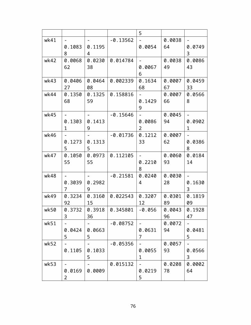
5wk41 -

0.10838

-0.11954

-0.13562 -0.0054

0.003864

-0.07493

wk42 0.006862

0.023038

0.014784 -0.00676

0.003849

0.008643

wk43 0.040627

0.046408

0.002339 0.163468

0.000767

0.045933

wk44 0.135068

0.132559

0.158816 -0.14299

0.000766

0.05668

wk45 -0.13031

-0.14139

-0.15646 -0.00862

0.004594

-0.09021

wk46 -0.12735

-0.13135

-0.01736 0.121233

0.000762

-0.03868

wk47 0.105055

0.097355

0.112105 -0.22108

0.006093

0.018414

wk48 -0.30397

-0.29829

-0.21581 0.02404

0.003028

-0.16303

wk49 0.323492

0.316015

0.022543 0.320712

0.030189

0.181909

wk50 0.37323

0.391836

0.345801 -0.056 0.004396

0.192847

wk51 -0.04245

-0.06635

-0.08752 -0.06317

0.007294

-0.04815

wk52 -0.1105

-0.10335

-0.05356 -0.00551

0.005793

-0.05663

wk53 -0.01692

-0.0009

0.015132 -0.02195

0.020878

0.000264

76

77