Exploring pre-main-sequence variables of the ONC: the new variables

arX

iv:0

907.

4836

v1 [

astr

o-ph

.SR

] 28

Jul

200

9

Mon. Not. R. Astron. Soc.000, 1–?? (....) Printed 12 December 2013 (MN LATEX style file v2.2)

Exploring pre-main sequence variables of ONC: The new variables

Padmakar Parihar1⋆, Sergio Messina2†, Elisa Distefano2‡, Shantikumar N.S.1§, and Biman J. Medhi1Indian Institute of Astrophysics, Bangalore 560034, India2INAF-Catania Astrophysical Observatory, Italy3Aryabhatta Research Institute of Observational Sciences (ARIES), Manora Peak, Nainital -263129, India

Accepted ..... Received ......; in original form .....

ABSTRACT

Since 2004, we have been engaged in a long-term observing program to monitor youngstellar objects in the Orion Nebula Cluster. We have collected about two thousands framesin V, R, and I broad-band filters on more than two hundred nights distributed over five con-secutive observing seasons. The high-quality and time-extended photometric data give us anopportunity to address various phenomena associated with young stars. The prime motiva-tions of this project arei) to explore various manifestations of stellar magnetic activity in veryyoung low-mass stars;ii) to search for new pre-main sequence eclipsing binaries; andiii) tolook for any EXor and FUor like transient activities associated with YSOs. Since this is thefirst paper on this program, we give a detailed description ofthe science drivers, the obser-vation and the data reduction strategies as well. In addition to these, we also present a largenumber of new periodic variables detected from our first five years of time-series photometricdata. Our study reveals that about 72% of CTTS in our FoV are periodic, whereas, the per-centage of periodic WTTS is just 32%. This indicates that inhomogeneities patterns on thesurface of CTTS of the ONC stars are much more stable than on WTTS. From our multi-yearmonitoring campaign we found that the photometric surveys based on single-season are inca-pable of identifying all periodic variables. And any study on evolution of angular momentumbased on single-season surveys must be carried out with caution.

Key words: Open clusters and associations: individual:Orion Nebula Cluster− stars: rota-tion: − stars: variable− stars: pre-main sequence− stars: activity− stars: late-type stars−stars: spots.

1 INTRODUCTION

The Orion Nebula Cluster (ONC) is an excellent target for study-ing young stellar objects (YSOs). It contains a few thousands ofpre-main sequence (PMS) stars within∼15 arc-minutes (2 pc) ofthe central Trapezium stars (Herbig & Terndrup 1986; Hillenbrand1997; Hillenbrand & Hartmann 1998). At a distance, 450±70 pc,ONC is the nearest high-mass star-forming region where one canfind very massive stars of∼25 solar mass (θ1 Ori C) to sub-solarobjects having mass well below the hydrogen burning limit (Hillen-brand 1997; Lucas & Roche 2000). From recent studies, it appearsthat formation of stars in the ONC started about 10 Myr back and,in the beginning, the formation process was very slow. Later, due tolarge scale contraction in the ONC parental cloud, the activity wentthrough a rapid phase of star formation. The mean age of the ONC

⋆ E-mail: [email protected]† E-mail:[email protected]‡ E-mail:[email protected]§ E-mail:[email protected]

is about 1 Myr, which characterizes an epoch when large fractionof stars were born. An age spread of 2 Myr around this mean age isfound by previous researchers (Hillenbrand 1997; Palla et al. 2005;Huff & Stahler 2006; Jeffries 2007). The ONC is located in front ofa very extended and fully opaque molecular cloud (AV peaks at 80-100 mag), which makes the background star contamination almostinsignificant in the optical region. This means that except for a fewforeground stars, all visible objects can be straight away consideredto be cluster members. Very intense radiation pressure and stellarwinds of the massive stars have cleared most of the dust from theONC (O’Dell 2001) and that is why about 80% cluster membersare subjected to relatively low visual extinction, AV ranging from0.0 to 2.5 mag (Hillenbrand 1997). The low-mass ONC stars arevery strong sources of X ray emission and the median luminosityof these objects is LX ∼ 30.25 erg sec−1 (LX/Lbol ∼10−3.5), which isthree orders of magnitude more intense than the solar X-ray lumi-nosity (Flaccomio et al. 2003). Recent studies reveal that the X-rayluminosity of low-mass stars increases with the stellar mass and de-creases with the age, but it seems to be independent of the rotation

http://arxiv.org/abs/0907.4836v1

2 Padmakar Parihar, et al.

period (Flaccomio et al. 2003; Stassun et al. 2004; Preibisch et al.2005).

In the past, for more than one decade, the ONC and the re-gions close-by (ONC flanking fields) were photometrically mon-itored by various researchers with varying degree of sensitivity aswell as spatial coverage (Mandel & Herbst 1991; Attridge & Herbst1992; Eaton et al. 1995; Choi & Herbst 1996; Stassun et al. 1999;Herbst et al. 2000; Carpenter et al. 2001; Rebull 2001; Herbst etal. 2002). Except the long-term observing program of Herbstandcollaborators of Van Vleck Observatory (VVO) and near infra-red(NIR) survey carried out by Carpenter et al. (2001), other moni-toring programs were primarily focused on a single goal and thatwas to explore the evolution of angular momentum of the starsin the PMS phase, by determining the rotation periods from thelight curves produced by modulation of light due to hot/cool spots.We realized that moderate size telescopes equipped with wide fieldimaging camera can be very effectively used to address a variety ofvaluable scientific problems related to PMS stars. And henceusingvarious observing facilities accessible to our group, since January2004 we have initiated a long-term monitoring program on thePMSstars of the ONC. Since this is the first paper on this project,we notonly report the results on the identification of new periodicvari-ables but also describe the science drivers, the observation and thedata reduction in some more detail. In Sect. 2 we describe oursci-entific motivations. Sect. 3 describes the selection of the target fieldand the observations. The data reduction procedures are describedin Sect. 4 together with the tools used to determine very accuraterotation periods. In Sect. 5 we present the results on the newly dis-covered periodic variables. A brief discussion and our planfor thenear future are given in Sect. 6.

2 SCIENTIFIC MOTIVATIONS

2.1 Exploring magnetic activities in T Tauri stars

T Tauri stars (TTS) are low-mass pre-main sequence objects andbased on the strength of the Hα line emission they are dividedmainly into two sub classes: weak lined TTS (WTTS) and clas-sical TTS (CTTS). The periodic photometric variability of WTTSis linked with rotational modulation of cool magnetic star-spots.Doppler Imaging, which is a robust stellar surface mapping tech-nique, supports the cool spot model (Strassmeier 2002; Schmidt etal 2005; Skelly et al. 2008). WTTS are found to be relatively fastrotators with the preliminary indication that they do not possesssurface differential rotation (Cohen et al. 2004; Skelly et al. 2008).They are sources of strong non-thermal radio as well as X-rayemis-sion. Since T Tauri stars are believed to be fully convective, theycannot sustain the so-calledαω interface dynamo. Furthermore, afossil field can survive only over timescales from 10 to 100 yearsin a fully convective star. So, even for few-million-year-old TTS, adynamo process is necessary to generate and amplify the magneticfield. The mechanism under which fully convective stars succeedto produce magnetism and related activities is a subject of debate(Chabrier & Kuker 2006 and references therein). The long-termmonitoring of low-mass stars of the ONC will be very valuabletounderstand the mechanism responsible for the generation ofmag-netic field in fully convective very young stars. We are particularlyinterested to explore the presence/absence of activity cycles and ofsurface differential rotation in WTTS.

CTTS are surrounded by a circum-stellar accretion disk andare characterised by the presence of strong emission lines as well

as an excess hot continuum emission. According magnetosphericmodels, strong dipolar field disrupt the inner disk at a few stellarradii. The disk material is channeled from the inner region of thedisk onto the star along the magnetic field lines. The free fallingmaterial eventually hit the stellar surface and develops accretionshocks (Calvet & Gullbring 1998). The thermalized shock energyform hot spots/ring near the magnetic pole which is seen as an ex-cess blue continuum emission in the spectrum of cool CTTS andin the optical-band photometry. The surface magnetic field mea-sured from Zeeman broadening in several CTTS indeed indicatesthe presence of very strong magnetic fields with an average fieldstrength of∼2.5 kG (Johns-Krull 2007; Bouvier et al. 2007). Re-cent results from the Zeeman Doppler Imaging technique alsore-veal the presence of large-scale dipolar fields of about 1 kG togetherwith a rather complex field configuration close to the stellarsurface(Jardine et al. 2008; Donati et al. 2008). The hot spots are supposedto be foot prints on the photosphere of the large scale dipolar field,which facilitates the accretion from the disk. From our long-termmulti-band monitoring program we intend to explore the temporalevolution of the hot spots. In addition, to obtain the disk accretionrate, we plan to model the CTTS light curves using star-spot models(Budding 1977; Dorren 1987; Mahdavi & Kenyon 1998) combinedwith the mechanism proposed by Calvet & Gullbring (1998) to ac-count the excess emission coming from the hot spots.

2.2 Search for PMS eclipsing binaries

Eclipsing binary systems provide an opportunity to measurestel-lar masses, radii, effective surface temperature, and luminosity ofthe individual components with very high precision. These are theparameters one need to test various theoretical PMS evolution-ary models. Several monitoring programs on young clusters,con-ducted recently by different groups have yielded only five suchPMS eclipsing binaries (Irwin et al. 2007; Cargile 2008 and ref-erences therein). Therefore, the identification of more such sys-tems is indeed in great demand. It appears that the discoveryofjust five eclipsing binaries among few thousand of PMS stars mon-itored so far, points toward the presence of some biases. Thefirstthing we must take into account is that most of the surveys made inthe recent past were single observing run, whereas the prominentsource of variability in low-mass PMS stars are either due totheinhomogeneous distribution of cool/hot spots and/or to the vari-able disk extinction. Therefore, the shallower light variation dueto the eclipses, being superimposed on these strong variations, islikely to be masked and only by means of repeated observationscarried out over several seasons one can disentangle these effects.Moreover, all PMS eclipsing systems identified so far are Algol-type eclipsing variables. The close semidetached/contact binaries(if they can form) and partially eclipsing variables are simply in-discernible from single season light curves, and hence not havebeen identified so far. Therefore, from our continuous multi-yearmonitoring, we expect to identify a few more interesting candidatesprobably missed out by previous surveys.

2.3 Studying other interesting variables

UXor objects are mostly intermediate-mass PMS stars but canalsobe low-mass PMS stars. The light curves of these stars are charac-terized by sudden drops in brightness up to 3 mag in the V band,followed by increased reddening and linear polarization (Waters &Waelkens 1998; Grinin et al. 1998; Herbig 2008). In very deepmin-ima the star reverses the color variation and, often, becomes bluer

Exploring pre-main sequence variables of ONC: The new variables 3

again (Bibo & The 1991). The origin of the brightness drops, theincrease in polarization, and the blueing effect have been debatedfor a long time (Natta et al. 1997; Bertout 2000; Dullemond etal.2003). The model based on variable obscuration suggest two dif-ferent mechanism: passage of proto-cometary clouds in front of thestar (Grady et al. 2000), and/or small hydrodynamic perturbationsin the puffed-up inner rim (Dullemond et al. 2003, Pontoppidan etal. 2007). On the other hand, a very interesting mechanism wasproposed by Herbst & Scevchenko (1999), in which unsteady ac-cretion naturally explains several observable phenomena related toUXor. From several Hα surveys including our own, we find aboutone hundred stars surrounded by the active accretion disk inoursmall FOV (Sect. 5.1), and it is quite expected that a few of thesewill indeed turn out to be UXor candidates.

FUor and EXor are young low-mass stellar objects surroundedby proto-planetary accretion disk and characterized by sudden en-hancement in the luminosity. During eruption, an FUor star can bebecome 100 to 1000 times more luminous and, then after it grad-ually fades up, reaching a quiescence phase. On the other hand,EXor phenomenon is found to be less energetic but shows morefrequent/recurrent transient activity. Both FUor and EXor phenom-ena are generally explained in terms of enhancement of disk accre-tion rate and several mechanisms have been proposed to trigger theoutburst. These include a tidal interaction with a companion star,thermal or gravitational instabilities, and induced accretion due topresence of massive planets (Bonnell & Bastien 1992; Hartmann etal. 2004; Vorobyov & Basu 2005; Lodato & Clarke 2004). It is alsonot well understood whether the physical mechanism operating inEXor outburst is the same as in FUors and the difference in burstduration as well as the amplitude is a consequence of PMS evolu-tion, or some very different physical process is responsible for theEXor phenomenon. There is one already known EXor in our field(V1118 Ori) and we expect to identify a few more EXor and FUorobjects.

In addition to identifying such a new objects, our multi-bandtime series data together with the spectroscopic follow-upstudywill greatly help to understand the mechanism responsible for theUXor, FUor and EXor phenomenon.

2.4 The angular momentum evolution in the PMS phase

In addition to the above mentioned science objectives, our programwill also be useful to address a few important aspects of the an-gular momentum evolution in the PMS phase. It is believed thata fraction of low-mass stars surrounded by disks goes through aphase of strong disk-braking, then after the disk-free starfreelyspins-up. The disk-braking models combined with the process ofstar formation (burst/sequential) as well disk dispersal, predict thebi-modal distribution of the rotation periods in young stars. How-ever, numerous studies made on this regard over the last decadeended-up with very contradictory claims and counter claims(Stas-sun et al. 1999; Herbst et al. 2002; Rebull 2004; Lamm et al. 2005,Rebull 2006; Cieza & Baliber 2007). In most studies of stellar an-gular momentum, the stellar rotation period is obtained from lightcurves produced by the rotational modulation of the star light due toinhomogeneous cool/hot spots, unevenly distributed on the stellarsurface. However, there have been no attempts made to check thecompleteness of the rotation periods derived from the lightcurvesof various objects (except some work done by Cohen et al. 2004on IC348; Lamm et al. 2005 on NGC2264). It is well known thatthe cool spots on WTTS and other active stars can change theirsizeas well as spatial distribution so dramatically and rapidlythat one

can not expect to get always the rotation modulation, specificallywhen the amplitude of variation is small. That is the reason,for ex-ample, why the single-season survey made by Herbst et al. (2002)in 1998-1999 with the MPG/ESO 2.2m telescope could not detectall the bright periodic variables identified by the previoussurvey ofStassun et al. (1999), despite using a larger telescope and,hence,with better sensitivity and accuracy. On the other hand, stars withdisks (mainly CTTS) are supposed to have both cool and hot spots.These stars usually display very irregular light variations and, of-ten, it is difficult to get their rotation period accurately, at least froma single observing run (Herbst et al. 1994; Grankin et al. 2007). Oneof the question we want to address is why just about 10-20% of sev-eral thousands of low-mass PMS stars monitored so far are foundto be periodic variables. What happened to the remaining 80-90%of stars? Why do they not show any regular and periodic variationdespite having all the ingredients to produce magnetic spots? So,our long-term monitoring program hopefully will put us in the po-sition to shed some light on detectability of the rotation periods andthe effects of biases preventing their detections.

3 SELECTION OF THE FIELD AND OBSERVATION

3.1 The selection of the field

Keeping in mind the science goals mentioned in the precedingsection, we started looking for a stellar field associated with veryyoung stellar clusters containing a large number of confirmed andrelatively bright young members confined to a small region. An-other criterion was that the field must have a large number of al-ready known PMS variables, representing to different mechanismsresponsible for the light variations. Our search finally ended on theONC, which was already chosen as target by other major moni-toring programs, conducted by Stassun et al. (1999), Herbstet al.(2000), Rebull (2001), Carpenter et al. (2001), and Herbst et al.(2002). More importantly, since 1990 hundreds of bright stars ofONC have also been continuously monitored by Herbst and hiscollaborators of VVO. The field of view (FOV) of the telescopeswhat we planned to use was 10×10 arc-minutes. Since our pro-gram needs long-term monitoring at least in two broad-band filters,and considering the limited availability of the telescope time, wehad to further optimize a very potential 10×10 arc-minutes fieldhaving large number of variables along with other measured quan-tities, such as NIR as well as X-ray data. We identified a regionsouth west of the Trapezium stars shown in Fig. 1. The coordinateof the selected ONC field isα(2000.0)= 05:35:04.09,δ(2000.0)=−05:29:04.8. We deliberately kept the very bright trapeziumstarsout of the field, so that the strong scattered light and very severebleeding of the charge should not spoil the CCD frame. The ONCfield chosen by us includes 110 periodic variables already knownfrom the literature: 92 from Herbst et al. (2000, 2002) and 38starsfrom Stassun et al. (1999, hereafter called S99), where 20 peri-odic variables are common in both groups. The cross-correlation ofoptically-identified stars from Hillenbrand (1997), with 2MASS allsky catalogue of point sources (Cutri et al. 2003) and COUP X-rayobservation (Getman et al. 2005), revealed that almost all opticalstars have NIR counterparts and large number of them have X-raydata as well. Most of these objects are low-mass stars and extremelyyoung candidates. Almost one fourth of our FOV is so close toTrapezium and severely affected by a strong HII region ( see Fig.1),whose average background level is several times larger thanin theregion slightly away from it. Nonetheless, we included thisregion


Figure 1. A 30×30 arc-min red band image from DSS on which the 10×10arc-min region chosen for the long-term monitoring is marked.

because it hosts a large number of relatively young low-massstars(younger than 1 Myr) and most of them have been found to besource of strong X-ray emission. Furthermore, it also comprises alarge number of intermediate-mass stars (Hillenbrand 1997).

3.2 Photometric Observations

The photometric observations of the ONC reported here, wereob-tained between January 18, 2004 and April 15, 2008, using the2m Himalayan Chandra Telescope (HCT) and the 2.3m VainuBappu Telescope (VBT). The Himalaya Faint Object Spectrograph(HFOSC) of HCT used in imaging mode uses 2k×2k central regionof 2k×4k CCD and covers a field of view of 10× 10 arc-minutes,with a scale of 0.296 arc-sec/pixel. The 1k × 1k CCD mounted atthe VBT prime focus covers a slightly larger field (∼ 11×11 arc-minutes) with plate scale of 0.65 arc-sec/pixel. The time series ob-servations were made primarily through Bessel I & V broad-bandfilters. However, during the most recent observing run (2007-08)we collected time series observations in R band too. The mostcom-plete time series data in all observing runs is in I band. Reasons togive more emphasis to I band are: (i) the I band minimizes the effectof nebular background and interstellar extinction, as wellit maxi-mizes the S/N of red faint stars which constitute the bulk of thecluster population, (ii) past monitoring programs were conductedprimarily in I band and so the comparison and the use of earlierdata is only possible with I band, and finally (iii) the effect of theseeing is least in I band, and the effect of color dependent atmo-spheric extinction, which is difficult to correct, is also minimized.In order to avoid the degradation of seeing at low elevation,effortwas also made to obtain photometric observations at low air-mass.Whenever possible, immediately after I band observations,we alsotried to collect V & R band data with motivation to get the colorcurves of at least a few bright and less embedded cluster members.During the observing rus 2004-06, whenever telescope time wasavailable, a sequence of 3-5 frames in each I and V filters withthe

Table 1.Log of the observations made to date.

Cyc Start Cyc End Filter No. Frames No. Nights

Jan 18, 2004 Feb 16, 2004 I 121 16V 69 14

Oct 11, 2004 Jan 26, 2005 I 109 25V 80 22

Aug 26, 2005 Dec 22, 2005 I 89 21V 58 19

Nov 28, 2006 Apr 07, 2007 I 337 57V 159 38

Aug 25, 2007 Apr 18, 2008 I 492 89V 274 35R 198 50

exposure time of 60 and 180 seconds were collected. In order to in-crease the dynamic range as well as the photometric measurementaccuracy of faint stars, starting from the most recent observing run(2007-08) we changed the observing strategy. Now, one shortex-posure is accompanied by 3-4 long exposures (20 and 90 secondsin I band, 60 and 300 seconds in V and R bands). Whenever possi-ble, this observing sequence which finally gives one averaged datapoint was repeated more than once per night. In total the ONC fieldwas observed on 208 nights and collected 1986 frames in R, V andI bands. A brief log of our observations is given in Table 1 andthedistribution of the nightly observations for all the filtersis shownin Fig. 2. The median seeing in I band for these observations is∼1.5 arc-sec (FWHM) and, during the course of our observations,it varied from 0.8 to 2.5 arc-sec. Seeing at shorter wavelengths wasslightly degraded according to the law of the wavelength dependentseeing (FHWM∝ λ−1/5).

Since accurate flat fielding is of critical importance in differ-ential photometry too, therefore, on every night we tried tocollecta large number of evening and morning sufficiently-exposed twi-light flats. Since there is no over-scan region in the detector usedby us, several bias frames, spread over the night, were collected.It has been found that even after taking all sorts of precaution todo very accurate flat fielding, small errors of the order of 0.1to1.0% remain in the flat field (primarily due to non-uniform illumi-nation of the flat field and wavelength-dependent differential vari-ation in the quantum efficiency of the pixels). Furthermore, ourback-illuminated thin CCD chips on both telescopes suffer fromhigh spatial frequency fringing problem. The combination of thesetwo effects typically limits the achievable photometric accuracytoa few milli-magnitude (mmag) depending on the instrument used.In order to minimize these effects, throughout the observing run,we tried to keep the stars in our FOV at the same pixel on CCDchip. To do this we selected a moderately bright star as a referencestar and kept this star at reference pixel just before the closed loopguiding used to begin. During 90% of observations, all target ob-jects were kept within the 2-3 pixels on the CCD frames.

3.3 Slit-less spectroscopy

In order to identify stars which show Hα in emission, in a few ob-serving nights of 2006-07, when the seeing was relatively better,the ONC field was also observed using HFOSC in the slit-less spec-tral mode with a grism as dispersing element. In this mode a com-bination of the Hα broad-band filter (Hα-Br, 6100 - 6740Å) andGrism 5 were used without any slit. This yields an image where


.

2003-04

2004-05

2005-06

2006-07

2007-08

Figure 2. The distribution of the observed nights for all five cycles. Thered, green and blue colors represent the observation made with I, R and Vfilters, respectively.

the stars are replaced by their low-resolution spectra, which are onaverage displaced by 163 pixels upward in the CCD plane. The2048×2500 pixels, central region of the 2k×4k CCD was used fordata acquisition. The average dispersion of Grism 5 around Hα is3.12 Å/pixel and the seeing was around 1.2 arc-sec (∼4 pixels),which sets the system resolution at about 500. Several repeated ob-servations with 600 second were made on each night and bias aswell as twilight flats were also taken on the same night with thesame setup. After bias correction and the flat fielding, as done inthe optical imaging, the spectral images were combined using me-dian combine. The consecutive spectral images were taken whileauto-guiding was active, so image shifts were found to be insignifi-cant and stellar spectra after median combine were found to be notsuffering through any smearing effect. On the other hand, we couldimprove not only the signal to noise ratio (S/N) in the median com-bined spectral image, but also remove the cosmic ray events andhence ensure unambiguous determination of sharp Hα emission.From the median combined image, strips of the image containingthe stellar spectra were copied and then the optimal extraction pro-cedures carried out in slit-spectroscopy were followed. Weused theIRAF taskapall to extract the spectra of 346 stars. A very accuratesky subtraction from those stellar spectra which have been affectedby the strong HII region is indeed very crucial. We sampled thesky from 2.5 arc-sec wide sky regions, nearly 2.5 arc-sec away,on either side of the stellar spectrum. To over come the problemof small scale strong variation in the sky background, a low-orderpolynomial was used to fit the background across the dispersion.This technique ensures that the nebular contribution in theHα pro-file is negligible and the measured Hα emission is indeed comingfrom the star. The coarse wavelength calibration was done byus-ing the average dispersion of the Grism 5, where the center oftheHα line was used as a reference point (6562.8Å). The Hα emission

line stars were identified and the equivalent widths(EW) were mea-sured. The smallest EW measured from our slit-less spectroscopywas found to depend on both seeing condition and star’s apparentmagnitude. The later fixes the strength of the continuum, with re-spect to what we measure the EW of emission lines. On the seeingvalue smaller than 1.5 arc-sec, we could measure EW as small as1Å and this can also be considered the typical error in our EW forthe stars having well exposed continuum.

4 DATA REDUCTION

4.1 Pre-processing and selection of the target stars

The basic image processing, such as bias subtraction and flat-fielding, were done in a standard way using tasks available withinIRAF. In order to minimize the propagation of statistical errorswhile doing the bias subtraction and flat fielding, it is recommendedthat on each night one need to collect a large number of bias andflat frames . However, on average not more than 4-8 bias framesaswell as twilight frames could be collected, due to the constraint im-posed by long read-out time (∼ 80 sec) of the CCD used. Therefore,to minimize the effect of propagation of the statistical error a largenumber of bias and flat frames were collected from near-by nightsand, depending on the stability of the features on the frames, biasand flats of 3 to 4 consecutive nights were combined to constructthe master bias and flat frames. After the bias correction andthe flatfielding, the next task was to identify a large number of sufficientlybright stars in our field. To do this we selected one I-band framewhich was obtained at fairly good seeing condition and used thedaofindtask of IRAF to identify stars within it. The radial profileof individual object was checked and the false detections orpro-file featuring extended objects were rejected. A total of 346objectssuitable for time series study were identified in this reference frame.Although the whole frame is affected to some extent by nebulosity,however, based on the intensity of the background emission we di-vided our FoV into three different sections, clear sky, sky partiallyaffected by nebula and the region where the nebula is very strong.The stars falling in these regions were marked with the sky flags,SC, SPN and SN. In addition to this a SNB flag is used for brightstars located in the region where the nebular emission is strong.Nearly 5% of the frames taken under very poor sky transparency orworst seeing condition or affected by strong wind were rejected forsubsequent analysis.

The astrometric calibration of the stars identified in the ref-erence frame discussed above was done using theStarlink pack-age ASTROM (Wallace 1994). The calibration was done using thecoordinates of about one hundred stars listed in the 2MASS cata-logue (Cutri et al. 2003) as references and on average the accuracyachieved on stellar coordinates is about 0.2 arc-sec. From the com-parison with various coordinates reported by earlier researchers, itappears that our coordinates very well match with the coordinatesof Herbst et al. (2002), with average difference of 0.23±0.21 arc-sec. Whereas, systematic 0.68±0.15 arc-sec and 1.39±0.28 arc-secdifferences have been noticed with Hillenbrand (1997) and S99.Herbst et al. (2002) also reported such difference and it was foundto be systematic errors in the astrometric transformation carried outby above two surveys.


4.2 The photometry

Despite our effort to keep our program stars always at the sameCCD pixel, the observed frames were found to be typically outofthe place and shifted with respect to the reference frame by 1to 3pixels. Furthermore, there were about 10% of the frames in whichthe effort was not made to center the star at the reference positionon the CCD. So, before we start the photometric reduction we hadtwo options. One possibility was to align all the frames withrespectto a reference frame and to use the same coordinates obtainedfromreference frame to all the frames. The other possibility wasto con-vert the coordinates of the stars determined from referenceframetaking the image shift as well as the rotation into account. We optedthe later procedure because the first procedure uses the intensity in-terpolation for the fractional shift in pixels and may not conservethe flux. The center of tens of bright stars were obtained using theCCD data reduction package DAOPHOT-II (Stetson 1987; 1992).Then after, the Stetson’sdaomatchand thedaomasterprogramswere used to obtain reasonably good transformation relation of stel-lar positions between the reference frame and any other observedframe. In the subsequent step the transformation relation generatedby daomasterwas used to generate an input coordinate file of all346 stars whose coordinates have been already determined inthereference frame. This coordinate file was used as input to eitheraperture photometry carried out by thephot task of IRAF or thePSF photometry done using Stetson DAOPHOT-II.

For each star we performed both aperture as well as PSF pho-tometry. In aperture photometry, the magnitude of stars were deter-mined with aperture radius spanning the range of 4-10 pixels. Keep-ing relatively poor seeing in consideration (FWHM varies from 4to 9 pixels), the sky was estimated from an annulus with slightlylarger inner radius of 30 pixels (∼ 8.8 arc-sec) and width of 10 pix-els. We played with various sky estimation procedures available inthe IRAF and found that themodegives more precise sky value and,hence, less scattered light curves of non-variable stars. Therefore,the sky was always estimated by using themodeoption, whenever,aperture photometry was carried out. The PSF photometry wasper-formed by modeling the star’s profile with a Penny-2 function. Weused this function because we found it yield a least residualaftersubtracting fitted stars from the image. Besides the analytical func-tions, which are used for the fitting procedure, another importantparameter of PSF photometry is the fitting-radius. For each framewe used a fitting-radius equal to the mean FWHM of the stellarprofiles. Such a value was about 4 pixels for the images acquiredin good seeing and about 8 pixels in poor seeing conditions. If anyfaint object has bright neighbours, then the effects of variable see-ing combined to the intrinsic variability of the bright neighbourscan introduce spurious variations. Such close pairs were identifiedand their time series photometric data was treated with special care.On total we identified 17 such pairs which have been found to beseparated by less than 6 arc-sec.

4.3 Ensemble differential photometry

The differential photometry was performed using the technique ofensemble photometry (Gilliland & Brown 1988; Everett & How-ell 2001; Bailer-Jones & Mundt 2001). In ensemble photometrythe differential magnitude is computed with respect to the aver-age magnitude of a large number of non-variable reference stars.The advantage of this technique is that, in the averaging process,the uncertainties of the ensemble stars magnitudes due to statisti-cal fluctuations as well as short-term small incoherent variations

will cancel each other. The uncertainty in the magnitude of the ar-tificial comparison, therefore will be smaller than the uncertaintyon the magnitude of a single star and this, in turn, will produceless noisy light curves. The ensemble photometry was performedwith ARCO, a software for Automatic Reduction of CCD Obser-vations, developed by us (Distefano et al. 2007). This software al-lows us to select automatically the suitable stars for the ensem-ble, i.e., sufficiently bright and isolated stars, which are commonto all the frames, and distributed all over the frame but not foundto be close to the CCD edges. After selecting the ensemble stars,ARCO automatically computes: (i) the magnitude of the artificialcomparison star by averaging instrumental flux of ensemble stars,(ii) time-series differential magnitudes for each star of the field and(iii) mean, median and the standard deviation (σ) associated to eachtime series. While computing the average ensemble magnitude, wefirst determined the average flux of all ensemble stars and, then af-ter, the ensemble magnitude was computed from the average flux.This way of computing ensemble magnitude gives more weight tothe bright stars which are expected to have smaller error related tophoton noise.

The whole procedure described above is iterative and startwith a large number of bright stars distributed all over the frame,excluding stars very much affected by the nebulosity. While con-structing the ensemble, the program exclude those ensemblestarswhose standard deviation is larger than the threshold sigmavaluefixed by the user. The final output of the software is a file with dif-ferential time-series magnitudes for all stars in the field includingthe ensemble stars. We used the ensemble made up of 24 stars togetdifferential magnitudes in I, R and V photometric bands. We run theprogram several times with different input data coming from aper-tures as well from PSF photometry and generated several setsoflight curves.

In principle, when differential aperture photometry is per-formed, the choice of the radius should not matter because, if thestellar profile does not vary significantly across the frame,the per-centage of the total flux collected through an aperture of a givenradiusr is same for all stars and, therefore, there should be no dif-ference between time-series data obtained with a 4-pixel apertureradius or with an 8-pixel radius. However, the use of a fixed radiusfor all stars is not recommended when the stars of the field spana broad range of magnitudes. Although a larger aperture increasesthe signal strength, however, at the same time, it increasesthe con-tribution of the noise due to the background fluctuations andCCDread out. In the case of bright stars the contribution to the totalnoise is mostly the photon noise whereas, the noise in the faint starmagnitude is due to the sky and read out noise of the CCD. So, alarge aperture is preferable to bright stars and a smaller aperture tofaint stars. It is well known that signal-to-noise ratio is afunctionof size of the apertures and is found to be maximum close the aper-ture radius of one FWHM of the stellar profile (Howell 1989). Themagnitude of faint stars may be very much affected even by slightinaccurate estimation of sky values and this can be minimized byadopting a small aperture. Whereas, any variation in the shape ofPSF over the frame introduces error in the bright stars magnitudes.Keeping all these in mind, a range of apertures starting from4 to 8pixels were used to generate the ensemble differential photometry.

As mentioned in Sect. 3, the differential ensemble magnitudesof the sequence of 3 to 4 frames collected within very short in-tervals of time (shorter than 1 hour) were combined and the meanvalue of the magnitudes from these close-by frames was used asone data point in the time series analysis. We also computed stan-dard deviation of these magnitudes which is a robust estimate of


Figure 3. The mean error associated to each data points as function of the Iband magnitude. The sequence which comprises the maximum distributionof the data points, were fitted with a piecewise function of second orderpolynomials and the exponential function. The data points of aperture radius6 has been only plotted here, but fitting were done for data of all threeapertures 4, 6 and 8 pixels radius and the best fit curves are shown here.Most of the deviant data points with respect to the fit, are associated withthe stars in strong nebula and hence the background photon noise are theprime source of the error.

the error associated with each data point. The mean of the standarddeviation< σ > is an average error of the measurement associatedwith any star which is a function of the magnitude and plottedinthe Fig. 3. Such an estimate of error linked with one data point isconservative because the true observational accuracy could be, inprinciple, even better for stars having substantial variability withinthe timescale close to our fixed binning time interval (i.e. 1hour).We have computed the mean error< σ > for all three aperturesof radius 4, 6 and 8 pixels, respectively. The lower bounds ofthedata points were fitted with a piecewise function of second orderpolynomials and the exponential function (see Fig. 3). As expected,the smaller apertures give better photometric precision tothe faintstars. Whereas, the large apertures seem to be more suitablefor thebrights stars. Relatively large errors associated with themagnitudesdetermined using small aperture of bright stars reflect the effect oftemporal as well as spatial variation of the PSF. The photometricprecision achieved in the interval of 11.5<I<16.0 is close to 0.01(∼1%) and then it degrades exponentially. During the final run ofthe photometric reduction, the optimum aperture was not only se-lected based on the stars brightness, but the aperture whichgivesthe lowest mean error (< σ >) was also taken in to account.

Finally, we performed a comparison between the results ob-tained from aperture photometry and from PSF-photometry. Sucha comparison is shown in Fig. 4, whereσ8 − σps f and σ4 −

σps f vs. I mag are plotted. In the fainter domain PSF-photometryis more advantageous than aperture photometry carried out with 8-pixel radius (Fig. 4). However, if the aperture photometry is done

-0.04

-0.02

0

0.02

0.04

11 12 13 14 15 16 17 18 19 20

σ 8 -

σps

f

I mag

-0.04

-0.02

0

0.02

0.04

11 12 13 14 15 16 17 18 19 20

σ 4 -

σps

f

I mag

Figure 4. In the top panel the quantity ”σ8 − σps f” vs. the I magnitude isplotted. The radius of 8 pixels gives a smaller standard deviation and, inturn, a less noisy light curve for brighter stars. To the fainter stars PSF pho-tometry seems to be advantageous, but looking at theσ4 − σPS F vs. I magplot (bottom panel), it appears that also in such a case aperture photometrygives the better results.

with radius of four pixels, then aperture photometry gives betterresults in the fainter domain (Fig. 4). From all these detailed exer-cise we found that in our case generally the aperture photometry ismore advantageous than PSF-photometry. Nevertheless, we foundthat there are few stars for which PSF-photometry produces lessnoisy light curves and we noticed that such stars are either closeto a brighter star or lying close to edges of the CCD. In such casesPSF-photometry is more efficient because it allows us to take intoaccount the effects of the distortion of the stellar profile at the edgesof CCD as well as it ”deblends” the star from the brighter neigh-bours. Therefore, to construct time series data of these stars we usedPSF-photometry.

4.4 Absolute Photometry

In order to obtain the standard magnitudes and the colors of alltargets in our FOV, which allow our observations to compare withprevious observations, we decided to carry out photometriccalibra-tion as precise as possible. The standardization of magnitudes alsoenables us to correctly place our objects in the HR diagram and todetermine various stellar parameters. On the six best nights of the2007-08 observing run, we observed a large number of BVRI pho-tometric standard stars from Landolt (1992) and deeper asterism ofM67 (Anupama et al. 1994). A few Landolt fields were monitoredover a wide range of air-mass to determine the nightly atmosphericextinction. From the extinction observation we found that only four


out of six nights were photometric and the transformation coeffi-cients were obtained from these nights. On the same night a largenumber of VRI frames with short and long exposures of the ONCwere taken, when it was close to the meridian. The short and longONC frames were aligned and then co-added separately, usingthemedian option of theimcombinetask of IRAF. The aperture pho-tometry magnitude with a radius of 1.5×FWHM, which is supposeto give maximum S/N was carried out for the all 346 ONC vari-ables. Then after, 20-30 fairly isolated bright stars free from neb-ulosity were used to determine the aperture correction. Finally theaperture corrected magnitudes of the ONC stars were obtained forthe aperture of 5×FWHM and then I-band magnitude and colorswere transformed using the transformation equation

I = i − ki X + ǫ(R− I ) + ζi (1)

(R− I ) = ((r − i) − kri∆ X)µri + ζri (2)

(V − I ) = ((v− i) − kvi∆ X)µvi + ζvi (3)

where k, X,ǫ, µ andζ are atmospheric extinction, air-mass, trans-formation coefficients, and zero points, respectively. The averagemagnitude and colors of all 346 stars were obtained from fournights using Eq. (1-3).

Finally, the accuracy of the photometric calibration was esti-mated by computing the standard deviation of magnitudes andcol-ors of the 24 comparisons used for the differential ensemble pho-tometry. And the errors were found to be 0.02, 0.04, and 0.05 magin I band, (R−I) and (V−I) colors, respectively. Because, nearly allstars in our field are expected to be variable with amplitude of vari-ability in the range from our accuracy limit (0.01mag) to fewtens ofmagnitudes, therefore, a better estimate of their brightness comesfrom the mean/median value of the time series data. Therefore,we determined the median magnitudes of each star’s time seriesdata collected over five consecutive observing years and comparedthese values with the I-band magnitudes of Hillenbrand (1997) andHerbst et. al (2002), the latter collected during a completeobser-vation season. The difference of the median magnitudes obtainedfrom the common stars are plotted against our I-band magnitude inFig. 5. Our median magnitudes and those from Herbst et al. (2002)seem to matching well, whereas, the difference with respect to Hil-lenbrand (1997) is quite apparent in the plot. Here we remindthat,differently than Herbst et al. (2002), the photometric data usedbyHillenbrand (1997) was mostly based on snapshot observations col-lected over few nights and hence affected by the intrinsic variabil-ity. The photometric data along with other relevant information ofall 346 stars in our FOV are partly given in Table 2, whereas, thecomplete table is available only electronically.

4.5 Search for periodicity

As already mentioned, one major objective of our project is to de-tect and characterize the optical and NIR band variability of all tar-gets detected in our FOV. Specifically, we aim at discoveringnewvariables and their rotation period whenever possible. Thevariabil-ity of low-mass members of ONC mostly arises from uneven dis-tribution of cool/hot brightness inhomogeneities on the stellar pho-tosphere, which, being carried in and out of view by the star’s ro-tation, produce a quasi-periodic variation in the observedflux. Thevariation in the star’s light is modeled through Fourier analysis todetermine the stellar rotation period. There are transientphenom-ena related to magnetic activity, such as flaring and micro-flaring,and star-disk interaction which also give rise to flux variability.

-2

0

2

12 14 16 18

-2

0

2

I (Mag)

Figure 5. The comparison of I-band magnitudes obtained from our pho-tometry and from Hillenbrand (1997), and Herbst et al. (2002). The meanand the standard deviations of the difference in magnitudes are also givenon the top of each plots.

However, they generally tend to be non-periodic, making more dif-ficult the detection of any periodicity in the observed time seriesdata. The reliable determination of the stellar rotation period is pos-sible if several conditions are met at a time. For example, stars musthave surface inhomogeneities unevenly distributed along the stellarlongitude, the stellar latitude of spots in combination with the incli-nation of the rotation axis must allow the rotation to modulate thespot visibility, and the inhomogeneity pattern must be stable overthe time interval when the photometric data are collected. Finally,the non-periodic phenomena mentioned earlier should not bedom-inant contributors to the flux variation. All these conditions are notalways satisfied.

Most of our targets are either WTTS or CTTS which show insome respects different patterns of variability. In the case of WTTS,the observed variability is dominated by phenomena relatedto mag-netic activity which manifest themselves on different time scales, asit also occurs in the more evolved MS and post-MS late-type stars(see Messina et al. 2004). The shortest time scale, of the order ofseconds to minutes, is related to micro-flaring activity. Its stochas-tic nature increases the level of intrinsic noise in the observed timeseries flux. The variability on time scales from several hours to daysis mostly related to the star’s rotation. Whereas, the variabilities onlonger time scales, from months to years, are related to the growthand decay of active regions (ARGD) as well as to the presence ofstar-spot cycles. In order to differentiate the effects on the variabil-


Table 2.The photometric data along with other relevant informationof all 346 stars in our FoV.

S.N. RA-Dec JW PHerbst PS tassun Sky Neighbour CTTS I R-I V-I Sp.Type J J-H H-K LX

161 05 34 55.006 -05 26 58.90 3111 - - SC - - 16.07 1.44 3.22 M5.5e13.83 0.92 0.61 29.00162 05 34 53.100 -05 26 59.54 - - - SC - - 18.61 3.60 2.67 - 15.96 0.79 0.35 28.04163 05 34 50.727 -05 27 01.01 117 8.870 - SC - C 13.17 1.02 2.10 M0e 11.65 0.93 0.53 29.26164 05 35 21.627 -05 26 57.78 688 - - SPN - - 14.68 0.74 2.81 - 12.84 0.76 0.31 29.10165 05 35 05.851 -05 27 01.64 281 3.160 - SPN - - 13.95 1.78 3.29 M3.5 12.10 0.96 0.32 29.56166 05 35 06.426 -05 27 04.82 290 - - SPN - - 15.37 1.56 3.81 - 12.93 0.74 0.48 29.41167 05 35 05.891 -05 27 09.00 283 7.010 - SPN - - 15.19 0.48 2.79 K8 12.51 1.37 0.75 29.72

NOTE: Only a portion of the table is shown here and complete table is available only in electronic edition of the MNRAS.

ity by ARGD and star-spot cycles from the effect of rotation, onwhich we are presently focused, we have analyzed our time seriesdata season by season from 2004 to 2008. Excluding cycle 5 whichis currently the longest one, we have collected our data during ob-servation seasons which are shorter than the timescale of ARGDtypically observed in PMS stars. In the case of CTTS, apart fromcool spots, also hot spots formed by accretion from the disk in-troduce additional variability. This type of variability is quite un-explored, in the sense that our knowledge either of the accretionprocesses or of their time scales is not as good as for WTTS. Weknow from previous studies that in most cases the combination ofdifferent mechanisms operating on different time scales makes thevariability highly irregular.

We included in our analysis also the data collected by Herbstet al. (2002) (hereafter referred to as H02), kindly made availableto us on our request. The independent analysis of the H02 datawith our tools (described in the following subsections), allowed usto check the reliability of our period search procedures. Wefirstsearched for the periodicity in our I band time series data collectedover all the seasons, because the I band data are more numerousthan V as well as R band data (see Fig. 2 and Table 1) and alsohave greater S/N ratio. Afterwards, the analysis of R and V bandtime series data was carried out to either confirm the periodicityfound from the I-band data and/or to search for additional periodicvariables.

We have used the Scargle-Press periodogram to search for sig-nificant periodicity. In the following sub-sections we briefly de-scribe our procedures to identify periodic variables amongour tar-gets.

4.6 Scargle-Press periodogram

The Scargle technique has been developed in order to search forsignificant periodicities in unevenly sampled data (Scargle 1982;Horne & Baliunas 1986). The algorithm calculates the normalizedpower PN(ω) for a given angular frequencyω = 2πν. The highestpeaks in the calculated power spectrum (periodogram) correspondto the candidate periodicities in the analyzed time series data. Inorder to determine the significance level of any candidate periodicsignal, the height of the corresponding power peak is related with afalse alarm probability (FAP), which is a probability that apeak ofgiven height is due to simply statistical variations, i.e. to noise. Thismethod assumes that each observed data point is independentfromthe others. However, this is not strictly true for our time series dataconsisting of data consecutively collected within the samenightand with a time sampling much shorter than the timescales of peri-odic variability we are looking for (Pd=0.1-20). The impact of thiscorrelation on the period determination has been highlighted by,e.g., Herbst & Wittenmyer (1996), S99, Rebull (2001) and Lammet al. (2004). In order to overcome this problem, we decided to de-

termine the FAP by different ways than proposed by Scargle (1982)and Horne & Baliunas (1986), the latter being only based on thenumber of independent frequencies. We followed the method optedby H02 (hereafter referred to asMethod A) and the approach pro-posed by Rebull (2001) (hereafter referred to asMethod B) .

4.6.1 Method A

Following the approach outlined by H02, randomized time seriesdata sets were created by randomly scrambling the day numberofthe Julian day (JD) while keeping photometric magnitudes and thedecimal part of the JD unchanged. This method preserves any cor-relation that exists in the original data set. We noticed that Lamm etal. (2004) in order to produce the simulated light curves, random-ized the observed magnitudes, instead of the epochs of observation.Then after, we applied the periodogram analysis to the ”random-ized” time series data for a total of about 10,000 simulations. Weretained the highest power peak and the corresponding period ofeach computed periodogram. In the top panel of Fig. 6, we plotthedistribution of detected periods from our simulations for I- banddata of the 5th cycle, whereas, in the bottom panel we plot thedis-tribution of the highest power peaks vs. period. The dashed lineshows the power level corresponding to the 99% confidence level.The FAP related to a given power PN is taken as the fraction ofrandomised light curves that have the highest power peak exceed-ing PN which, in turn, is the probability that a peak of this heightis simply due to statistical variations, i.e. white noise. We note thatsuch power thresholds are different from season to season, becauseof different time sampling, length of the observation season, andtotal number of data. The normalised powers corresponding to aFAP < 0.01 are reported in the second column of Table 3 for the5 observation seasons as well as the averaged H02 data. We notethat in our analysis we averaged the H02 time series data in thesame manner as done in our own time series (see Sect. 4.3). There-fore, the reduced total number of analysed data in each lightcurveleaded to a proportionally smaller power level - about 8.2 against16.5 for the unaveraged data as reported by H02.

4.6.2 Method B

Following the method given by Brown et al. (1996), synthetictimeseries data was generated with the same sampling as the observeddata and the frequencies were searched over the same range asdonewith the real data. The synthetic time series are built by using arandom number generator with a Gaussian distribution of points

xi>0 = αxi−1 + βR(0, σ) (4)

where x represents the magnitude of the light curve,α=exp(−∆t/Lcorr), where∆t is the time between magnitudes xi−1 and xi ,β=(1−α2)1/2, and R(0,σ) is the random number generator with a


Table 3.Normalized power at 1% FAP as established by randomizing timeseries (Method A) and by correlated Gaussian noise (Method B)

cycle Method A Method BLcorr(d)

0.0 0.1 0.25 0.5 1.0 2.0

PN PN PN PN PN PN PN

1 6.2 7.0 8.2 9.1 9.3 9.5 10.42 6.9 7.8 7.9 8.3 9.2 9.9 10.33 6.6 7.3 7.7 7.6 7.7 7.6 8.64 8.4 8.0 8.8 9.6 10.3 11.4 13.45 9.2 8.4 11.4 13.9 15.5 16.7 19.6

H02 (averaged) 8.2 7.8 8.2 8.8 9.4 10.4 12.8

dispersionσ, which is the variance of the time series data. The ini-tial mean magnitudex0 is selected via a call to R(0,σ). For moredetails on this procedure see Rebull (2001) and Brown et al. (1996).Lcorr = 0 d sets the case of uncorrelated Gaussian noise, where eachdata is assumed to be uncorrelated from others. A range of correla-tion time starting from 0.1 to 2 days were used. For each valueofcorrelation time we have built a set of about 10000 syntheticlightcurves and used the distribution of maximum power from the cor-responding periodograms to determine the 1% FAP. The results aresummarized in Table 3.

The increase of Lcorr implies that the synthetic light curves be-come more correlated and this makes the power level correspond-ing to any threshold FAP larger, which in turn increases the risk tomiss the detection of real periodicities. We found that a value ofLcorr=1.0d is a good compromise to properly account for the corre-lation in our data. For Lcorr >1.0d we start systematically missingeven those rotation periods whose reliability have been firmly es-tablished by previous multi-year surveys (e.g. H00).

We see that the power level adopted to discriminate periodicfrom non periodic target is larger than the values found bothinthe Method A and in Method B for uncorrelated Gaussian noise(Lcorr = 0.0d). Finally, we notice that these FAP values are con-servative. The reason is that even in the same observing run thesampling of the time series data differ from object to object. Thishappens primarily due to, objects close to the edge of the detectorwere some time missed out due to telescope pointing error, sometime at poor seeing faint objects failed to collect sufficient signaland hence undetectable. When doing our simulations we adoptedthe largest FAP level, which we generally found in the most nu-merous time series data (that is the case for more than 80% of lightcurves).

In order to establish whether a star can be considered a peri-odic at 99% confidence level we decided to adopt Method B forcorrelated Gaussian noise (Lcorr = 1.0d). All the stars listed in Ta-ble 6 satisfy this selection criterion. In a few cases, as shown in theon-line Figs.8-14, more than one peak were found with power ex-ceeding the fixed threshold value at 99%. These secondary peaksare generally alias of the peak related to the rotation period, whichis the only periodicity we expect in these late-type PMS stars inthe period range searched by us (0.1-20 days). In order to checkthat the secondary peaks are indeed nothing but an aliasing effectas well as to correctly identify the rotation period, we proceeded bysubtracting the smooth phased light curve of period associated withhighest peak. Then after, we re-computed the periodogram onthepre-whitened time series data. In most cases no significant peakswere left in the pre-whitened time series data with confidence levellarger than 99%. A total 14 stars whose rotation periods werede-

Figure 6. Distribution of periods (top panel) and power of the highestpeaks (bottom panel) resulting from Scargle periodogram analysis of10,000 ”randomised” light curves. Original time series data were col-lected during cycle 5 in the I band.

tected with a confidence level larger than 99% were excluded fromthe following analysis and not included in Table 6, since they dis-play very noisy phased light curves. These stars were also not iden-tified as a periodic variables by previous surveys.

4.7 Uncertainty with the rotation period

In order to compute the error associated with periods determined byus we followed the method used by Lamm et al. (2004). Accordingto this method the uncertainty in the period can be written as

∆P =δνP2

2(5)

whereδν is the finite frequency resolution of the power spectrumand is equal to the full width at half maximum of the main peakof the window function w(ν). If the time sampling is not too non-uniform, which is the case of our observations, thenδν ≃ 1/T,where T is the total time span of the observations. From Eq. 5 it isclear that the uncertainty in the determined period, not only dependon the frequency resolution (total time span) but is also proportionalto the square of the power. We also computed the error on the pe-riod following the prescription suggested by the Horne & Baliunas(1986) which is based on the formulation given by Kovacs (1981).We noticed that the uncertainty in period computed according toEq. 5 was found to be factor 5-10 larger than the uncertainty com-puted by the technique of Horne & Baliunas (1986). In this paperwe report the error computed with the first method described above.Hence, it can be considered as an upper limit, and the precision inthe period could be better than that we quote in this paper.

5 RESULTS

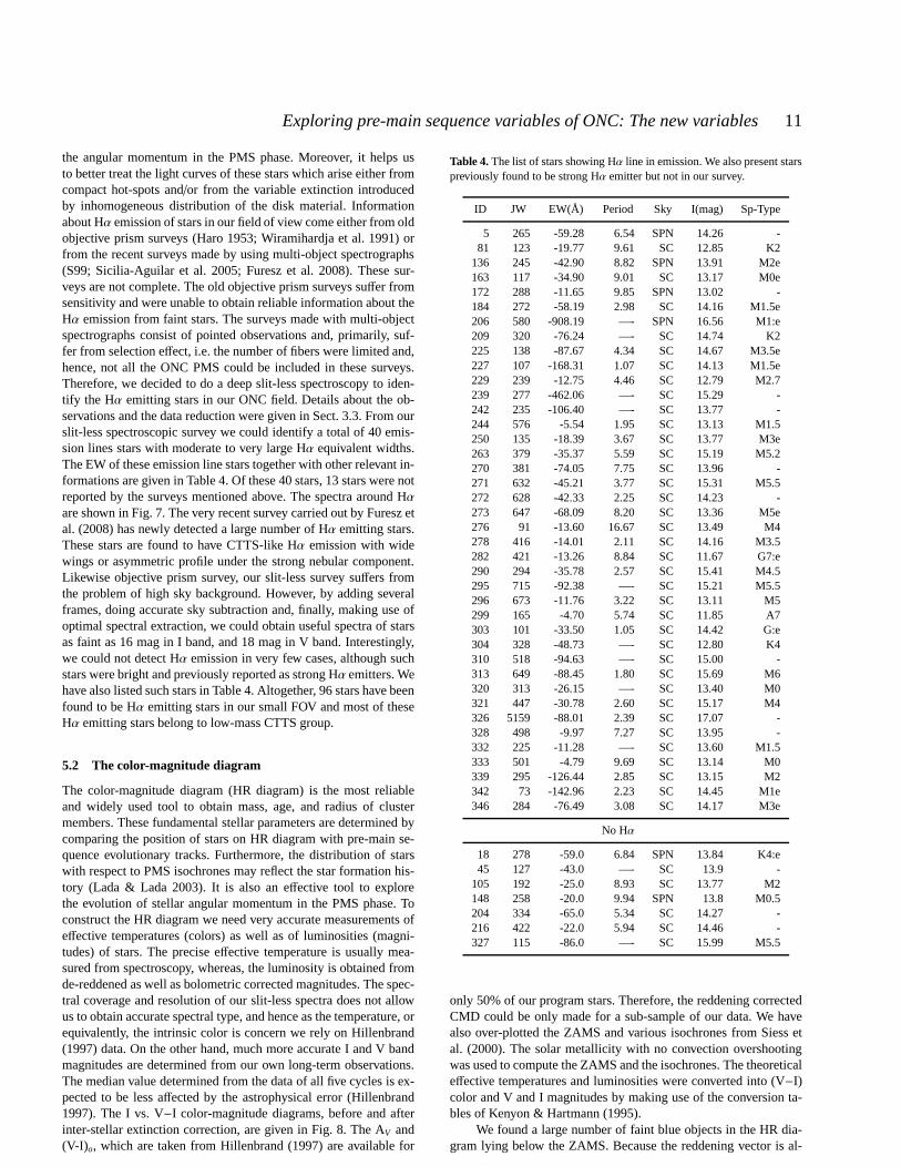
5.1 The Hα line emission stars

The strong Hα emission coming from low-mass PMS stars is anunambiguous signature of active accretion from the disk on to thesurface of star. Reliable knowledge of the presence/absence of aaccretion disk is desirable particularly for studying evolution of


the angular momentum in the PMS phase. Moreover, it helps usto better treat the light curves of these stars which arise either fromcompact hot-spots and/or from the variable extinction introducedby inhomogeneous distribution of the disk material. Informationabout Hα emission of stars in our field of view come either from oldobjective prism surveys (Haro 1953; Wiramihardja et al. 1991) orfrom the recent surveys made by using multi-object spectrographs(S99; Sicilia-Aguilar et al. 2005; Furesz et al. 2008). These sur-veys are not complete. The old objective prism surveys suffer fromsensitivity and were unable to obtain reliable informationabout theHα emission from faint stars. The surveys made with multi-objectspectrographs consist of pointed observations and, primarily, suf-fer from selection effect, i.e. the number of fibers were limited and,hence, not all the ONC PMS could be included in these surveys.Therefore, we decided to do a deep slit-less spectroscopy toiden-tify the Hα emitting stars in our ONC field. Details about the ob-servations and the data reduction were given in Sect. 3.3. From ourslit-less spectroscopic survey we could identify a total of40 emis-sion lines stars with moderate to very large Hα equivalent widths.The EW of these emission line stars together with other relevant in-formations are given in Table 4. Of these 40 stars, 13 stars were notreported by the surveys mentioned above. The spectra aroundHαare shown in Fig. 7. The very recent survey carried out by Furesz etal. (2008) has newly detected a large number of Hα emitting stars.These stars are found to have CTTS-like Hα emission with widewings or asymmetric profile under the strong nebular component.Likewise objective prism survey, our slit-less survey suffers fromthe problem of high sky background. However, by adding severalframes, doing accurate sky subtraction and, finally, makinguse ofoptimal spectral extraction, we could obtain useful spectra of starsas faint as 16 mag in I band, and 18 mag in V band. Interestingly,we could not detect Hα emission in very few cases, although suchstars were bright and previously reported as strong Hα emitters. Wehave also listed such stars in Table 4. Altogether, 96 stars have beenfound to be Hα emitting stars in our small FOV and most of theseHα emitting stars belong to low-mass CTTS group.

5.2 The color-magnitude diagram

The color-magnitude diagram (HR diagram) is the most reliableand widely used tool to obtain mass, age, and radius of clustermembers. These fundamental stellar parameters are determined bycomparing the position of stars on HR diagram with pre-main se-quence evolutionary tracks. Furthermore, the distribution of starswith respect to PMS isochrones may reflect the star formationhis-tory (Lada & Lada 2003). It is also an effective tool to explorethe evolution of stellar angular momentum in the PMS phase. Toconstruct the HR diagram we need very accurate measurementsofeffective temperatures (colors) as well as of luminosities (magni-tudes) of stars. The precise effective temperature is usually mea-sured from spectroscopy, whereas, the luminosity is obtained fromde-reddened as well as bolometric corrected magnitudes. The spec-tral coverage and resolution of our slit-less spectra does not allowus to obtain accurate spectral type, and hence as the temperature, orequivalently, the intrinsic color is concern we rely on Hillenbrand(1997) data. On the other hand, much more accurate I and V bandmagnitudes are determined from our own long-term observations.The median value determined from the data of all five cycles isex-pected to be less affected by the astrophysical error (Hillenbrand1997). The I vs. V−I color-magnitude diagrams, before and afterinter-stellar extinction correction, are given in Fig. 8. The AV and(V-I) o, which are taken from Hillenbrand (1997) are available for

Table 4.The list of stars showing Hα line in emission. We also present starspreviously found to be strong Hα emitter but not in our survey.

ID JW EW(Å) Period Sky I(mag) Sp-Type

5 265 -59.28 6.54 SPN 14.26 -81 123 -19.77 9.61 SC 12.85 K2

136 245 -42.90 8.82 SPN 13.91 M2e163 117 -34.90 9.01 SC 13.17 M0e172 288 -11.65 9.85 SPN 13.02 -184 272 -58.19 2.98 SC 14.16 M1.5e206 580 -908.19 —- SPN 16.56 M1:e209 320 -76.24 —- SC 14.74 K2225 138 -87.67 4.34 SC 14.67 M3.5e227 107 -168.31 1.07 SC 14.13 M1.5e229 239 -12.75 4.46 SC 12.79 M2.7239 277 -462.06 —- SC 15.29 -242 235 -106.40 —- SC 13.77 -244 576 -5.54 1.95 SC 13.13 M1.5250 135 -18.39 3.67 SC 13.77 M3e263 379 -35.37 5.59 SC 15.19 M5.2270 381 -74.05 7.75 SC 13.96 -271 632 -45.21 3.77 SC 15.31 M5.5272 628 -42.33 2.25 SC 14.23 -273 647 -68.09 8.20 SC 13.36 M5e276 91 -13.60 16.67 SC 13.49 M4278 416 -14.01 2.11 SC 14.16 M3.5282 421 -13.26 8.84 SC 11.67 G7:e290 294 -35.78 2.57 SC 15.41 M4.5295 715 -92.38 —- SC 15.21 M5.5296 673 -11.76 3.22 SC 13.11 M5299 165 -4.70 5.74 SC 11.85 A7303 101 -33.50 1.05 SC 14.42 G:e304 328 -48.73 —- SC 12.80 K4310 518 -94.63 —- SC 15.00 -313 649 -88.45 1.80 SC 15.69 M6320 313 -26.15 —- SC 13.40 M0321 447 -30.78 2.60 SC 15.17 M4326 5159 -88.01 2.39 SC 17.07 -328 498 -9.97 7.27 SC 13.95 -332 225 -11.28 —- SC 13.60 M1.5333 501 -4.79 9.69 SC 13.14 M0339 295 -126.44 2.85 SC 13.15 M2342 73 -142.96 2.23 SC 14.45 M1e346 284 -76.49 3.08 SC 14.17 M3e

No Hα

18 278 -59.0 6.84 SPN 13.84 K4:e45 127 -43.0 —- SC 13.9 -

105 192 -25.0 8.93 SC 13.77 M2148 258 -20.0 9.94 SPN 13.8 M0.5204 334 -65.0 5.34 SC 14.27 -216 422 -22.0 5.94 SC 14.46 -327 115 -86.0 —- SC 15.99 M5.5

only 50% of our program stars. Therefore, the reddening correctedCMD could be only made for a sub-sample of our data. We havealso over-plotted the ZAMS and various isochrones from Siess etal. (2000). The solar metallicity with no convection overshootingwas used to compute the ZAMS and the isochrones. The theoreticaleffective temperatures and luminosities were converted into (V−I)color and V and I magnitudes by making use of the conversion ta-bles of Kenyon & Hartmann (1995).

We found a large number of faint blue objects in the HR dia-gram lying below the ZAMS. Because the reddening vector is al-


Figure 7. The spectra around Hα from slit-less spectroscopic observations made on February 07, 2007 using HFOSC.

most parallel to ZAMS as well as the isochrones, so even afterred-dening correction these stars will not fit to any of the isochrones.Hillenbrand (1997) also found such blue and less-luminous objectsand inferred that they may be either heavily veiled CTTS and/orstars buried in nebulosity. Strongly veiled stars can become sys-tematically bluer by 1-2 mag in (V−I) color. However, at the sametime they should also be strong Hα emitters, which is indicative ofstrong active disk accretion, that has not been found exceptfor fewobjects. On the other hand, there is a large number of such blue faintstars lying in the intense nebulosity. Since the average color of theONC nebula close to the Trapezium is about V−I=0.11 mag, there-fore, it is likely that these stars appear bluer due to nebular con-tamination. These two phenomena can not explain all the outliers.Moreover, there are a few faint blue non-accreting stars outside thestrong nebulosity. These objects may not be at all stellar objects orthey may be UX Ori objects, which have been found to be bluerwhen they become fainter. Most of these faint blue objects werenot observed spectroscopically by Hillenbrand (1997) and hencethey simply disappear in the reddening corrected CMD. It also ap-pears from the uncorrected CMD that CTTS are more populous inthe upper portion of the PMS sequence than WTTS. This indicatesthat accreting CTTS are in general younger than WTTS. But anysuch trend disappears in the reddening corrected CMD. In agree-ment with earlier studies, the mean age of ONC appears to be ofabout 1 Myr with an age spread of about 3 Myr in the uncorrectedCMD. Here, we assume that the reddening vector is almost parallelto the isochrones in the low-mass range and that the reddening cor-rection will not change the relative distribution of the stars. In thereddening corrected CMD, ONC appears slightly older (∼2 Myr).This apparent difference in the age could be due to incompletenessof the reddening corrected sub-sample.

5.3 Periodic variables

The results of our search for periodic variables are presented in thissubsection. As mentioned, we searched for rotation periodsby an-alyzing our own data collected in five consecutive observation sea-sons as well as H02 data. Only stars having a peak power in the pe-riodogram, larger than 99% confidence level computed accordingto Method B for correlated Gaussian noise, were selected as ape-riodic variables. (see Sect. 4.6.2). In Table 6 we report theinforma-tion related to only the season in which the rotation period has beendetermined most precisely. Table 6 lists the following information:our star identification number (ID) which runs from 1 to 346; anidentification number from Hillenbrand (JW number); the normal-ized power (PN) of the highest peak in the Scargle power spec-trum, and the rotation period together with its uncertainty(P±∆P).In the next columns we list the reduced chi-squares (χ2

ν) of the lightcurve computed with respect to the median seasonal magnitude andthe average precision (< σ >) of the time series data computed asdescribed in the Sect. 4.3. Then we list the amplitude of the lightcurves in I band (∆I), which was computed by making the differ-ence between the median values of the upper and lower 15% ofmagnitude values of the light curve (see, e.g., H02). That allows usto prevent overestimation of the amplitude due to possible outliers.After this, we list the number of total useful observations and thedata points after averaging the close observations. In the next threecolumns of Table 6 we put the following notes: n1 denotes the sea-son to which the listed period and all the values in the previouscolumns refer; n2 denotes the cycles where the same periodicity,approximately within the computed uncertainty, were found(’H’stands for H02 and H00 data, ’S’ for S99 data, ’all’ for all cyclesincluding H02, H00 & S99 data); n3 indicates whether the staris a’new’ periodic or a previously known periodic variable whose pe-riod is in agreement or disagreement with the one determinedby


(V-I)

Figure 8. The color-magnitude diagram of ONC stars without reddeningcorrection is shown in the top panel. The bottom panel shows the same diagramafter reddening correction. Filled and open data points represent stars inside or outside nebulosity, respectively. The circles represent CTTS and other stars aremarked by a triangle.

Table 5.Result of the periodogram analysis of periodic variables ofthe ONC.

ID JW Power P±∆P χ2ν < σ > ∆I # # # n1 n2 n3 Sky Object Type Neighbour

(d) (mag) (mag) obs. mean dis.

5 265 45.59 6.540± 0.100 73.17 0.041 0.34 230 61 2 c4 c3/c5/H new SPN C y15 710 15.68 7.810± 0.180 106.99 0.231 1.43 76 25 2 c2 c1/H =S SC C -16 349 50.41 9.250± 0.120 173.62 0.054 0.63 397 101 6 c5 c3/c4 new SNB - -17 125 16.71 8.860± 0.150 86.95 0.010 0.11 74 21 2 c3 c1/c4 new SC C -18 278 60.60 6.840± 0.060 4189.88 0.016 1.60 400 102 6 c5 all =H SPN C -23a 366 18.86 8.790± 0.230 36.30 0.026 0.16 97 29 1 c2 - =H SNB - -27 437 31.38 2.341± 0.008 11.60 0.018 0.09 180 88 5 c5 H =H SNB C -29 417 15.58 7.370± 0.100 7.64 0.035 0.08 75 21 1 c3 c1/H =H SNB C -31 622 19.93 3.770± 0.150 52.29 0.032 0.26 365 105 4 c5 c1/H new SNB - -34 81 25.05 4.400± 0.040 26.53 0.010 0.12 62 21 2 c4 c1/c2/c3/H =H SC W -35 9213 21.64 12.220± 1.410 16.13 0.039 0.34 103 21 1 c1 c3 new SNB - y40 317 6.33 8.080± 0.190 14.37 0.018 0.08 97 29 3 c5 c2 =H SNB - -

NOTE: Only a portion of the table is shown here and complete table is available only in electronic edition of the MNRAS.a: The rotation period was detected in only one season and, although with a FAP< 1%, it needs to be confirmed by future observations.b: The rotation period, although detected in multiple seasons and with a FAP< 1%, may be a beat period, being very close to the window function main peak.

Stassun (S) or Herbst (H). Then after the position of stars with re-spect to the nebulosity (Sky), the star classification as CTTS (C) orWTTS (W). Finally, the last column denotes the presence (y) of an-other star closer than 6 arc-sec. In Fig. 9 we plot, as an example, theresult of our periodogram analysis obtained for one of our targetsID=293 which has been identified as periodic variable.

As listed in Table 6, there is a large number of stars whose

rotation period has been detected in all observing seasons includ-ing H02 data as well. The periodogram analysis performed on thewhole 5-yr time series allows us to determine the rotation periodswith accuracy better than 1%. Although the study of the long-termbehaviour of our targets will be the prime subject of a subsequentpaper, we show in Fig. 10 the light curves of one of these stars(ID=202), as an example. This example light curves show two in-


Figure 9. Results of periodogram analyses on the newly discovered periodic variable ID=293. Top panel:I-band time series data from cycle 4. Differentsymbols are used to better distinguish three different time intervals within the same observations season.Middle panels : Power spectra from Scargle analysis.The horizontal dashed line indicates the 99% confidence level, whereas the vertical dotted line marks the detected periodicity. Bottom panelphased light curveusing the detected period.

teresting features. The first is that within the longest observing run(season 5), the light curve is very smooth and the shape has re-mained constant over about 5 months. This indicates that thesizeas well as the distribution of the spot which modulates the star lightremain unchanged. This behaviour differs from what is observed inMS stars of similar rotation period, whose spot patterns arefoundto be stable over periods not longer than 1 to 2 months. However,we stress that this is the case for a limited number of stars inoursample, whereas there is a large number of stars whose rotation pe-riod, although detected in cycle 5 data, was not detected when thewhole time series data was analysed. This is likely due to a rapidchange of the spot pattern on these stars. Another feature isthechange in amplitude, mean light level and migration of the lightcurve minimum from season to season. These latter variations maybe related to the the presence of surface differential rotation (SDR)and ARGD.

As already mentioned, a part of our ONC field has been pho-tometrically monitored since 1990 at Van Vleck ObservatorybyHerbst and collaborators (see, e.g., H00), in 1994 by S99, and in1998-1999 by H02 at the MPG/ESO 2.2m telescope. Our analy-sis allowed us to identify a total of 148 periodic variables:56 arethe periodic stars newly discovered by us, whereas 92 were alreadyknown from the mentioned previous surveys (24 from Herbst andcollaborators, 11 stars from S99, and 57 from both groups). We didnot detect any periodicity in 18 stars, of which 2 were previouslyreported as periodic variables only by S99 (star 302 and 342)and16 only by Herbst and collaborators (star 3, 4, 38, 39, 62, 69,94,114, 129, 152, 175, 208, 302, 327, 339, and 344). Actually, wenotethat previous surveys could detect the periodicity for 14 out of these18 stars in only one observation season, hence their classification as

Figure 10. Example of light curves of one of our CTTS targets (ID=202)whose rotation period was detected in all our 5 observation season and inthe Herbst et al. (2002) data as well.


a periodic variables can be considred tentative. Among the 92 starswith already known rotation period, there are 14 stars for which wedetect a period different than that previously reported. However, wecould understand the origin of the disagreement. For 5 stars(star81, 96, 135, 181, 307), the rotation periods reported by either H02or S99 are very different from ours. Looking at our periodogramsof H02 averaged data we found a major power peak at the sameperiod found in multiple seasons in the power spectra of our timeseries. However, such peaks have a power slightly smaller than thethreshold (PN=16.5) that they fixed and, therefore, they were notconsidered in the H02 sample. Indeed, this is an example of the ad-vantage of multi-season with respect to single-season observationsto obtain more reliable rotation periods.

For the stars 240, 254, 283, 296 we found a period that is al-most doubled from the period reported by H02 or S99. This mis-match can be explained by considering that, at that time whenthesestars were observed, two major spots were located on opposite stel-lar hemispheres, giving rise to a flux modulation with half the pe-riod we found.

The disagreement to 4 stars (star 44, 285, 293, 303) is likelydue to the beat phenomenon, ours or the H02 and S99 periods be-ing beats of the true period. For star 274 we found in all seasonstwo different periods, one in common with H02 & S99 and anotherdifferent. We adopted the latter, since it gives less scattered phasedlight curves.

Therefore, we can state that for 92 periodic stars, the resultsof our period search well conciliate with the results of previousstudies. This point is very important, since it assures thatwe havebeen indeed collecting very precise photometric data as well as us-ing a reliable period analysis technique. In addition to this we getconfidence on our new detection of periodic variables and also con-firmation of the previous findings. We have discovered 56 new pe-riodic variables in our very small 10×10 arc-min FOV and henceincreased the total number of known periodic variables by almost50%. However, we must note that 7 new periodic stars (identifiedwith an apex ’a’ in Table 6) were detected as periodic for the firsttime by us and in only in one season. We need additional observa-tions to confirm these periodicities, which will be considered at thepresent as tentative and will not be included in any subsequent anal-ysis or statistics. For instance, the number of periodic stars whoseperiod is detected in only one season (∼ 5%) is similar to the to-tal number of false detections expected in 5 observation seasons byfixing the FAP at 1%. We must consider with great caution also the2 new periodic stars identified with an apex ’b’ in Table 6, sincetheir period is very close to 1 day. Although, the same periodwasdetected in multiple seasons, with high confidence level andgivingsmooth light curves, it may be an alias arising from the observa-tion day-night duty cycle. They also will not be considered in thefollowing analysis. The complete sample of light curves of our pe-riodic variables are plotted in Figs. 13-17. In these figureswe plotonly one light curve per star, specifically the details of which hasbeen listed in Table 6.

There are very few massive early spectral type stars in ourFoV. Since such objects are saturated, almost all our program starsare low- to very low-mass objects and we treat them as TTS. Inour FOV, till to date, 96 stars are found to show the Hα line inemission and with very large EW, hence, these stars can be assumedas accreting CTTS. Whereas, the remaining 242 stars which lackthe Hα emission can be considered as WTTS. These numbers ofCTTS and WTTS should be considered a preliminary estimate, andlikely subjected to be changed in the future. In fact, as mentioned inSect. 5., a few stars which were reported by previous studiesas Hα

emission stars, are found by us with no emission, whereas 13 newlyHα emitting stars have been identified by us. Thus, it appears thatto identify all accreting CTTS using Hα emission as a proxy, moreextensive multi-year spectroscopic survey is needed. Moreover, wenote that a few stars (like star 16, 41, 297 and 309) show an I-band light curve amplitude larger than 0.5 mag, although we havenot detected Hα emission. Such large amplitude most likely arisesfrom the presence of both hot spots and variable extinction by thecircum-stellar disk. Keeping these numbers distribution of WTTSand CTTS, our period search shows that about 72% of CTTS areperiodic variables. Whereas, the percentage of periodic WTTS isabout 32%. Our findind is contrary to Lamm et al. (2004), whoseresults on photometric monitoring of NGC2264 reveal that 85%WTTS and 15% CTTS are periodic variables.

From our study it appears that the detection of periodic sig-nal related to rotation is easier in CTTS than in WTTS. This issurprising in the sense that, as mentioned previously, it isbelievedthat the variability of CTTS is dominated by non-periodic phenom-ena, which should often prevent the detection of any periodic signalcoming from the rotation (Herbst et al. 1994; Lamm et al. 2004).From the present study, it appears that the CTTS of ONC have pat-terns of surface inhomogeneities which give rise to the flux varia-tions more stable than in WTTS and much more than in MS starsof similar period (see Fig. 10 as one example of stable CTTS lightcurve). The increased ability to detect rotation periods inCTTSmay be due to the large amplitude of light modulation, a charac-teristic of CTTS. That compensates to some extent the presence of”noisy” non-periodic phenomena, allowing the periodogramanaly-sis to correctly identify the rotation period. The other possibility isthat the number of CTTS identified from various Hα emission sur-veys has been underestimated, and actual number of Hα emittingCTTS are larger than the total number of 96 what we used for thecalculation.

As we mentioned earlier, we have divided our entire FOV inthree different regions and the number of spatial distribution of to-tal as well as periodic variables are as follows. There are 59starsresiding in bright nebular region and designated as SNB, 98 starsare in partially nebular region (SPN), 189 are outside the nebula(SC). We could determine the rotation period of 27% (16/59) starsinside the nebula, of 33% (33/98) partially in the nebula, and of52% (99/189) outside the nebula. As expected, the detection of pe-riodic variables outside nebulosity, where the backgroundlight con-tribution is minimum and the photometric accuracy better, is muchhigher than inside nebulosity. Another possibility could be the pres-ence of a large number of intermediate mass stars, inside thenebula,which are known for their irregular photometric behaviour.Finally,it was also found from previous studies that low-mass stars insidethe Trapezium cluster are relatively younger (Hillenbrand1997).Hence, it is quite possible that the youthness of these objects maketheir variability rather irregular.

The part of our FOV is very much affected by the presenceof strong HII nebular emission and, hence, the background con-tribution is very high. In addition to this as mentioned earlier thedistribution of the stellar mass as well as age are not uniform inthis region, therefore, we attempted to get some information aboutthe spatial distribution of periodic variables. In Fig. 11 we plot thespatial distribution of periodic variables over the FoV. The unex-pected result what we find is that the detection frequency of the ro-tation period, i.e. number of seasons on which any object hasbeenidentified as periodic, is indistinguishable from inside tooutside ofthe nebula. This result is surprising because the fact that inside thenebula, the observed magnitudes of stars are subjected to the lower


0 500 1000 1500 20000

500

1000

1500

2000

X (in pixels)

1c 2c 3c 4c 5c 6c 7c

Figure 11.The spatial distribution of periodic variables. Open circle represent the periodic variable detected from our long-term monitoring program. Whereasthe detection frequency is represented by size of the open circle, i.e. the largest circle correspond to the periodic variables, detected in all cycles including theprevious surveys by Herbst et al. (2002) and Stassun et al. (1999). The green color represent the CTTS stars identified from Hα emission and the red colorrepresent WTTS and/or other unclassified stars found to be periodic.

photometric precision, objects are relatively massive andtheir agerelative to the mean cluster age is less.

5.4 Scarcity of short period variables

During cycles 4 and 5, we dedicated a number of nights to searchfor very fast rotating periodic variables. In order to make our timeseries data sensitive to very short-term flux modulations down toabout 0.1 days, we monitored the ONC field over several full nights.Again, the data collected within one hour were combined and usedas one single data point while doing time series analysis. Thesemore numerous data collected within the same night allowed us tovery accurately identify 22 periodic variables with periodshorterthan about two days, 5 of which were newly identified by us. Wecould also identify 2 new variables having periods very close toone day. These short period variables are reported in this paper be-cause they have been detected in multiple seasons with high con-fidence level. However, their period need to be confirmed sincethey may be alias arising from the observation day-night duty cy-cle. The scarcity of very fast rotators (P<0.9d) in the magnituderange (12<I<17) explored by our survey supports the S99 findingon short-period variables. He first noticed that the ultra fast rota-tors that have been found in the Pleiades or in other older clus-

ters are quite absent in the ONC, at least in the 12<I<17 magni-tude range. This finding is quite expected for the low-mass starsof 1 Myr, whose break-up velocity is close to 0.5 days. However,here we like to emphasize that the fastest rotating stars identified byus in our FOV show a period about two times longer than S99. Incontrast, after a few Myrs, like in NGC 2264, the number of rota-tors faster than 0.4 days increases rapidly. A very deep photometricmonitoring campaign recently carried out by Rodriguez-Ledesmaet al. (2008) in the ONC, shows the presence of very fast rotators(P>0.5d) among Very Low Mass Stars (VLM) and sub-stellar ob-jects (BDs). These very fast rotating VLM and BDs probably pos-sess different dynamo mechanism, operating in this mass regimeand producing magnetic fields of different strength and topology aswell (Herbst et al. 2006).

5.5 Non-periodic targets

We never detected evidence of periodic variability in 198 out of 346stars. We have computed for each season the reduced chi-square(χ2ν) with respect to the seasonal median light level in order to quan-

tify their level of variability. Theχ2ν of each star is found to vary

from season to season. Their mean values vs. the median I mag-nitude (top panel) and vs. our internal ID number (bottom panel)


Figure 12. Top panel:Distribution of reduced chi-squares vs. I magnitude. Filled and open symbols are used to distinguish periodic from non periodicvariables, whereas different color indicate the star’s position with respect to thenebula.Bottom panel:reduced chi-squares vs. internal ID number.

are plotted in Fig. 12. The dashed vertical bars connect the mini-mum and maximumχ2

ν values ever observed. The red, green andblue colors indicate the target position with respect to thenebula(inside, partially inside and outside, respectively). Filled and openbullets represent periodic and non periodic variables, respectively.

Except the stars 230 and 308, which are the least variable inour sample, all non periodic targets can be classified as variable,havingχ2

ν > 3 in at least one season. This is not a surprising find-ing since all targets are very young stars. They host numerous phe-nomena which induce variability in the optical as well as in otherbands. Interestingly, theχ2

ν show a spatial dependence: their val-ues monotonically decrease from inside to outside the nebula. Thiseffect does not depend on the star’s brightness, as shown in thetop panel of Fig. 12, but more likely on mass and age. As men-tioned, a previous study (Hillenbrand 1997) shows a concentrationof intermediate-mass stars inside the nebula, which are character-ized by very irregular and large-amplitude variability. Itis alsoquite possible that stars inside nebula are younger and, therefore,being more active give rise to a larger-amplitude variability.

6 DISCUSSION AND PLAN FOR NEAR FUTURE

The luminosity spread in the color-magnitude diagram for starshaving similar color, and hence mass, has been generally associatedwith the age spread and found to be an effective tool to explore thestar formation history in young clusters (Hillenbrand 1997; Palla &Stahler 2000; Hartman 2001). However, limited photometricmea-

surement accuracy, intrinsic variability and effect of binarity in themagnitudes can mask the signatures of the initial age spread. Theuse of the median magnitude from our long-term photometric mon-itoring of the ONC stars has allowed us to construct a CMD muchmore accurate than in previous studies, mostly based on snapshotobservation, and, hence, has allowed us to better asses the pres-ence/absence of any age spread in the ONC. It is quite apparent inthe CMD of Fig. 8 that, after reddening correction, both WTTSandCTTS indeed show a spread in the magnitude at any color, whichpossibly points toward the presence of an age spread. However, wecan not draw a very firm conclusion on this because of the smallsize of our sample and possible effects from unrecognized binariesas well as uncertain extinction correction. The presence/absence ofspread in age of young stars has been subject of exploration overthe last decade and contradictory claims have been made (Hart-man 2001; Burningham et al. 2005; Jeffries 2007; Hillenbrand etal. 2008 and references their in). In near future, we expect to makefurther progress in our study on this subject by enlarging the sizeof our sample, identifying the binaries in our FOV as well as by abetter measurement of the intra-cluster extinction correction.

Our multi-epoch observations have allowed us to identify ina very small FOV a large number periodic variables (an additional50%). These newly identified periodic variables were unidentifiedmostly by previous surveys carried out over a single observing sea-son. If we exclude massive stars or stars highly affected by nebu-losity, then we found about 44% of stars in our FoV to be periodic.This is indeed a great gain with respect to previous surveys of S99


and H02 who discovered periodic variability only in 11% and 26%,respectively, of stars in our same FOV. Here we must keep in mindthat the S99 and H00 surveys were carried out with much smalleraperture telescopes, hence on a smaller sample of brighter stars.We could obtain agreement with previously determined periods in∼70% of stars, could explain the disagreement for 16% of peri-odic stars, whereas did not detect periodicity in the remaining 14%stars common in all these surveys. Our finding, and the results ofother ongoing multi-year surveys (e.g. H00) as well, pose a strongwarning about the completeness of the periodic variables discov-ered in young open clusters from single observing run, whichis themost common case. If we extend our finding to other star formingregions photometrically monitored in only one season, we expectthat the total number of periodic variables is highly underestimated.Therefore, when deriving any conclusion about the distribution ofrotation period and its implication to angular momentum evolution,the sample incompleteness must be seriously taken into account.

Our monitoring program together with two previous surveyshas yielded 148 periodic variables in a sample of 346 stars detectedin our FOV. Except few stars, which show no definite variability,all the other stars were found to be variables, although withno sys-tematic variations, i.e. irregular variables. It would be interestingto know what makes some stars periodic and others non-periodic.Is the undetected periodicity due to unfavourable inclination of therotation axis, which does not allow the spot pattern visibility to bemodulated? Or, is a very unstable spot pattern the major source ofirregular behaviours of these non-periodic variables? In addition tothese causes, sporadic accretion and extinction due to clumpy innerdisk could be the source of irregular variation in the stars classi-fied as a CTTS. We will be addressing all these questions in ourforthcoming papers.

7 CONCLUSIONS

Five consecutive years of observation of a 10×10 arc-minutes re-gion of the ONC, using moderate size telescopes has allowed us tofind several interesting results. We summarize our results below:

• We identified 13 new stars with moderate to strong Hα emis-sion, whereas, we did not detect emission in 7 stars, which werereported in the literature as strong Hα emitters.• The median multi-band magnitudes obtained from the long-

term time series data have allowed us to put stellar members onHR diagrams more accurately than the previous studies. Fromthecomparison with theoretical isochrones, it appears that the age ofONC is 1-2 Myr with a noticeable spread in the age.• Our multi-year monitoring has allowed us to detect 56 new

periodic variables, which increases by 50% the number of knownperiodic variables in the ONC region under study.• From a comparison with previously know periodic variables

we found matching periods for 70% variables. We find disagree-ment for 16% which can be explained either by period doublingoraliasing. To remaining 14% stars no period variation was detected.• We also find the absence of stars with period shorter than 0.9

days in the 1 Myr old, brights members ( 12<I<17 mag) of theONC.• Despite very high background emission, a large number of pe-

riodic variables have been identified inside the nebula. These starsdisplay a higher level of variability as for as reduced chi-square (χ2

ν)is concern.• Our study reveals that about 72% of CTTS in our FOV are

periodic, whereas, percentage of periodic WTTS is just 32%.This

indicate that inhomogeneity patterns on the surface of CTTSof theONC are much more stable than in WTTS.• All but two stars in our small FOV are found to be variable,

according to the chi-square criterion.

ACKNOWLEDGEMENTS

The Observations reported in this paper were obtained usingtwotelescopes of the Indian Institute of Astrophysics (Bangalore, In-dia): the 2-m HCT of Indian Astronomical Observatory (IAO),andthe 2.3-m VBT of Vainu Bappu Observatory (VBO) in Kavalur.We thank the staffs of IAO and VBO for their active support duringthe course of our observations. We are also very much grateful toProf. W. Herbst and Dr. K.G. Stassun who provided the raw dataoftheir photometric observations. This work has been also supportedby a grant given by the Department of Science & Technology In-dia and by the Italian MIUR (Ministero dell’Istruzione, Universitae Ricerca). The extensive use of the SIMBAD and ADS databasesoperated by the CDS center, Strasbourg, France, are gratefully ac-knowledged. Finally, we are indebted to our reviewer Prof. Herbstfor giving valuable suggestion/comments which immensely helpedus to improve the content of the manuscript.

REFERENCES

Anupama G. C., Kembhavi A. K., Prabhu T. P., Singh K. P., BhatP. N., 1994, A&AS, 103, 315

Attridge J. M., Herbst W., 1992, ApJ, 398, L61Bailer-Jones C. A. L., Mundt R., 2001, A&A, 367, 218Bertout C., 2000, A&A, 363, 984Bibo E. A., The P. S., 1991, A&AS, 89, 319Bonnell I., Bastien P., 1992, ApJ, 401, L31Bouvier J., Alencar S. H. P., Harries T. J., Johns-Krull C. M., Ro-manova M. M., 2007, prpl.conf, 479

Brown, Alexander, Deeney, Bryan D., Ayres, Thomas R., Veale,Anthony, Bennett, & Philip D., 1996, ApJS, 107, 263

Burningham B., Naylor T., Littlefair S. P., Jeffries R. D., 2005,MNRAS, 363, 1389

Budding E., 1977, Ap&SS, 48, 207Calvet N., Gullbring E., 1998, ApJ, 509, 802Cargile P. A., Stassun K. G., Mathieu R. D., 2008, ApJ, 674, 329Carpenter J. M., Hillenbrand L. A., Skrutskie M. F., 2001, AJ,121, 3160

Chabrier G., Kuker M., 2006, A&A, 446, 1027Choi P. I., Herbst W., 1996, AJ, 111, 283Cieza L., Baliber N., 2007, ApJ, 671, 605Cohen R. E., Herbst W., Williams E. C., 2004, AJ, 127, 1602Cutri R. M., et al., 2003, tmc..book,Distefano E., et al., 2007, EAS, 25, 165Donati J.-F., et al., 2008, MNRAS, 390, 545Dorren J. D., 1987, ApJ, 320, 756Dullemond C. P., van den Ancker M. E., Acke B., van Boekel R.,2003, ApJ, 594, L47

Duvert G., Guilloteau S., Menard F., Simon M., Dutrey A., 2000,A&A, 355, 165

Eaton N. L., Herbst W., Hillenbrand L. A., 1995, AJ, 110, 1735Everett M. E., Howell S. B., 2001, PASP, 113, 1428Furesz G., Hartmann L. W., Megeath S. T., Szentgyorgyi A. H.,Hamden E. T., 2008, ApJ, 676, 1109


Flaccomio E., Damiani F., Micela G., Sciortino S., Harnden F. R.,Jr., Murray S. S., Wolk S. J., 2003, ApJ, 582, 382

Getman K. V., et al., 2005, ApJS, 160, 319Gilliland R. L., Brown T. M., 1988, PASP, 100, 754Grady C. A., Sitko M. L., Russell R. W., Lynch D. K., Han-ner M. S., Perez M. R., Bjorkman K. S., de Winter D., 2000,prpl.conf, 613

Grankin K. N., Melnikov S. Y., Bouvier J., Herbst W., ShevchenkoV. S., 2007, A&A, 461, 183

Grinin V. P., Rostopchina A. N., Shakhovskoi D. N., 1998, AstL,24, 802

Haro G., 1953, ApJ, 117, 73Hartmann L., 2001, AJ, 121, 1030Hartmann L., Hinkle K., Calvet N., 2004, ApJ, 609, 906Herbig G. H., 2008, AJ, 135, 637Herbig G. H., Terndrup D. M., 1986, ApJ, 307, 609Herbst W., Herbst D. K., Grossman E. J., Weinstein D., 1994, AJ,108, 1906

Herbst W., Wittenmyer R., 1996, AAS, 28, 1338Herbst W., Rhode K. L., Hillenbrand L. A., Curran G., 2000, AJ,119, 261

Herbst W., Bailer-Jones C. A. L., Mundt R., Meisenheimer K.,Wackermann R., 2002, A&A, 396, 513

Hillenbrand L. A., Bauermeister A., White R. J., 2008, ASPC,384, 200

Hillenbrand L. A., 1997, AJ, 113, 1733Hillenbrand L. A., Hartmann L. W., 1998, ApJ, 492, 540Horne J. H., Baliunas S. L., 1986, ApJ, 302, 757Howell S. B., 1989, PASP, 101, 616Huff E. M., Stahler S. W., 2006, ApJ, 644, 355Irwin J., et al., 2007, MNRAS, 380, 541Jardine M. M., Gregory S. G., Donati J.-F., 2008, MNRAS, 386,688

Jeffries R. D., 2007, MNRAS, 381, 1169Johns-Krull C. M., 2007, ApJ, 664, 975Kenyon S. J., Hartmann L., 1995, ApJS, 101, 117Kovacs G., 1981, Ap&SS, 78, 175Lada C. J., Lada E. A., 2003, ARA&A, 41, 57Lamm M. H., Bailer-Jones C. A. L., Mundt R., Herbst W., ScholzA., 2004, A&A, 417, 557

Lamm M. H., Mundt R., Bailer-Jones C. A. L., Herbst W., 2005,A&A, 430, 1005

Landolt A. U., 1992, AJ, 104, 372Lodato G., Clarke C. J., 2004, MNRAS, 353, 841Lucas P. W., Roche P. F., 2000, MNRAS, 314, 858Mahdavi A., Kenyon S. J., 1998, ApJ, 497, 342Mandel G. N., Herbst W., 1991, ApJ, 383, L75Messina S., Rodono M., Cutispoto G., 2004, AN, 325, 660Medhi, Biman J., 2006, PhDT, 45MNatta A., Grinin V. P., Mannings V., Ungerechts H., 1997, ApJ,491, 885

O’dell C. R., 2001, ARA&A, 39, 99Palla F., Randich S., Flaccomio E., Pallavicini R., 2005, ApJ, 626,L49

Palla F., Stahler S. W., 2000, ApJ, 540, 255Pontoppidan K. M., Dullemond C. P., Blake G. A., BoogertA. C. A., van Dishoeck E. F., Evans N. J., II, Kessler-SilacciJ., Lahuis F., 2007, ApJ, 656, 980

Preibisch T., et al., 2005, ApJS, 160, 401Rebull L. M., 2001, AJ, 121, 1676Rebull L. M., Stauffer J. R., Megeath S. T., Hora J. L., HartmannL., 2006, ApJ, 646, 297

Rebull L. M., Wolff S. C., Strom S. E., 2004, AJ, 127, 1029YSC’15 Proceedings of Contributed Papers (eds. Choliy V. Ya.,Ivashchenko G.), 2008, pp. 21-24

Scargle J. D., 1982, ApJ, 263, 835Sicilia-Aguilar A., et al., 2005, AJ, 129, 363Siess L., Dufour E., Forestini M., 2000, A&A, 358, 593Skelly M. B., Unruh Y. C., Cameron A. C., Barnes J. R., DonatiJ.-F., Lawson W. A., Carter B. D., 2008, MNRAS, 385, 708

Stassun K. G., Ardila D. R., Barsony M., Basri G., Mathieu R. D.,2004, AJ, 127, 3537

Stassun K. G., Mathieu R. D., Mazeh T., Vrba F. J., 1999, AJ, 117,2941

Stetson P. B., 1992, ASPC, 25, 297Stetson P. B., 1987, PASP, 99, 191Strassmeier K. G., 2002, AN, 323, 309Vorobyov E. I., Basu S., 2005, ApJ, 633, L137Wallace P. T., 1994, ASPC, 61, 481Waters L. B. F. M., Waelkens C., 1998, ARA&A, 36, 233Wiramihardja S. D., Kogure T., Yoshida S., Nakano M., Ogura K.,Iwata T., 1991, PASJ, 43, 27


Figure 13. I-band light curves of our periodic variables vs. rotation phase. Phases are computed using the rotation period reported in Table 6. Different symbolsare used to disctinguish data belonging to different time intervals (see caption of Fig. 9. The solid line represents the sinusoidal fit to the data.


Table 6.Result of the periodogram analysis of periodic variables ofthe ONC.


(d) (mag) (mag) obs. mean dis.

5 265 45.59 6.540± 0.100 73.17 0.041 0.34 230 61 2 c4 c3/c5/H new SPN C y15 710 15.68 7.810± 0.180 106.99 0.231 1.43 76 25 2 c2 c1/H =S SC C -16 349 50.41 9.250± 0.120 173.62 0.054 0.63 397 101 6 c5 c3/c4 new SNB - -17 125 16.71 8.860± 0.150 86.95 0.010 0.11 74 21 2 c3 c1/c4 new SC C -18 278 60.60 6.840± 0.060 4189.88 0.016 1.60 400 102 6 c5 all =H SPN C -23a 366 18.86 8.790± 0.230 36.30 0.026 0.16 97 29 1 c2 - =H SNB - -27 437 31.38 2.341± 0.008 11.60 0.018 0.09 180 88 5 c5 H =H SNB C -29 417 15.58 7.370± 0.100 7.64 0.035 0.08 75 21 1 c3 c1/H =H SNB C -31 622 19.93 3.770± 0.150 52.29 0.032 0.26 365 105 4 c5 c1/H new SNB - -34 81 25.05 4.400± 0.040 26.53 0.010 0.12 62 21 2 c4 c1/c2/c3/H =H SC W -35 9213 21.64 12.220± 1.410 16.13 0.039 0.34 103 21 1 c1 c3 new SNB - y40 317 16.33 8.080± 0.190 14.37 0.018 0.08 97 29 3 c5 c2 =H SNB - -41b 3084 79.72 1.005± 0.001 93.87 0.165 1.07 410 106 8 c5 c1/c2/c3/c5 new SPN - -42 71 28.67 14.400± 2.400 16.90 0.013 0.11 103 21 1 c1 c4/c5/H new SC - -44 291 30.76 8.450± 0.210 5.93 0.009 0.04 223 61 2 c2 c4 ,H SPN - -51 658 28.97 3.204± 0.004 121.67 0.090 0.45 238 61 3 c4 c2/c3/c5 new SNB - -52 356 27.28 4.840± 0.260 45.21 0.008 0.08 103 21 1 c1 c3/c4/c5/H =H SNB - -54a - 15.30 9.460± 0.170 45.33 0.072 0.30 77 21 2 c3 - new SNB - -57 77 80.10 1.501± 0.004 47.05 0.013 0.19 245 62 2 c3 all =HS SC W -65 678 31.20 12.870± 0.240 120.88 0.073 0.45 203 93 3 c5 c4/H =H SNB W -66 130 22.84 1.206± 0.002 12.60 0.027 0.10 417 107 5 c5 all =H SC - -68 292 25.68 5.120± 0.070 31.56 0.019 0.18 97 29 3 c2 c1/c4/c5/H new SPN - -75 275 80.36 0.950± 0.001 18.84 0.014 0.09 411 107 6 c5 c1/c2/c4/H =H SPN - -78b 516 51.65 1.023± 0.001 45.39 0.035 0.26 415 107 4 c5 c1 new SNB - -81 123 37.80 9.610± 1.050 330.29 0.004 0.16 90 21 1 c1 all ,S SC - -88 323 54.49 11.370± 0.020 766.12 0.021 0.73 417 107 5 c5 c1/c2/c3 new SPN C -95 152 23.55 4.520± 0.240 9.61 0.006 0.03 103 21 1 c1 all new SC - -96 183 25.00 1.871± 0.005 9.05 0.007 0.03 103 21 1 c1 c3/c4/H ,H SC - -104 636 36.26 10.770± 1.320 133.92 0.012 0.22 101 21 1 c1 c2/c4/H =H SNB C y105 192 36.08 8.930± 0.230 1090.97 0.008 0.51 97 29 2 c2 all =S SC C -107 551 32.64 19.150± 4.190 24.69 0.010 0.09 103 21 1 c1 c5 new SNB - y109 535 36.81 18.170± 3.780 33.88 0.014 0.15 103 21 1 c1 c5 new SNB - -115 674 22.80 6.110± 0.070 139.90 0.014 0.30 62 20 2 c3 c1/c2/c4 new SNB - -117 299 28.69 2.770± 0.010 45.08 0.025 0.15 245 62 3 c4 c1 =H SPN C -118 3104 49.41 3.120± 0.020 55.95 0.033 0.28 97 29 2 c2 all =H SPN - -121 70 45.74 1.497± 0.005 19.48 0.011 0.09 246 62 4 c4 c1/c2/H =H SC - -122 250 30.21 2.740± 0.010 9.13 0.012 0.06 245 62 1 c4 all =H SPN - -125a 234 16.92 3.960± 0.040 7.01 0.016 0.05 97 29 2 c2 - new SPN - -130 324 27.69 6.250± 0.440 43.88 0.016 0.18 103 21 2 c1 c4/c5 new SPN C -131 254 21.10 3.500± 0.010 11.30 0.017 0.06 417 107 5 c5 c1/c2/H =H SPN - -133 104 58.44 1.772± 0.004 161.70 0.015 0.26 417 107 5 c5 c3/c4/H =H SC C -134 280 31.71 1.990± 0.010 10.55 0.008 0.04 96 29 2 c2 all =HS SPN - -135 - 19.17 3.620± 0.140 4.83 0.031 0.11 103 21 1 c1 H ,H SC - -136 245 43.45 8.820± 0.190 43.95 0.006 0.09 245 62 2 c4 c2/c5 =S SPN C -138 485 36.25 9.670± 0.270 205.72 0.013 0.29 97 29 2 c2 all =H SPN - -142 220 52.08 2.330± 0.010 15.02 0.005 0.05 208 58 3 c4 c1/H =H SPN C -145 168 34.51 0.912± 0.009 16.10 0.010 0.07 103 21 1 c1 c4/c5/H =H SC W -147 243 24.49 10.150± 0.300 52.89 0.006 0.10 97 29 1 c2 all =S SPN C -148 258 31.36 9.940± 1.130 76.22 0.006 0.11 103 21 1 c1 c4/c5/H =H SPN C -154 683 17.75 11.430± 0.190 12.92 0.028 0.13 205 91 2 c5 c4/H =H SPN - y158 573 55.73 4.750± 0.030 14.14 0.043 0.23 417 107 4 c5 c3 new SPN C -163 117 37.58 9.010± 0.500 10.08 0.010 0.06 244 62 2 c4 c1 =H SC C -165 281 29.75 3.150± 0.110 6.15 0.005 0.03 103 21 1 c1 c4/H =H SPN - -166 290 31.16 3.080± 0.010 45.72 0.009 0.12 103 21 2 c1 c3 new SPN - -167 283 35.35 7.390± 0.620 27.85 0.009 0.07 103 21 2 c1 c4/c5/H =H SPN - -170 392 16.05 3.900± 0.020 3.07 0.015 0.04 416 107 5 c3 c5 new SPN C -172 268 39.08 9.850± 0.140 69.50 0.016 0.15 417 107 4 c5 c1/c3/c4/H =H SPN C -173 477 39.36 6.670± 0.110 10.25 0.007 0.04 245 62 3 c4 c1/c3 new SPN - -174 415 16.75 2.060± 0.010 10.25 0.007 0.04 245 62 3 c2 c1 new SPN - -178 427 24.86 4.500± 0.060 15.82 0.008 0.05 97 29 2 c2 c1 new SPN C -181 144 27.78 3.960± 0.030 9.23 0.012 0.05 245 62 2 c4 c1/c3 ,H SC - -182 164 25.28 6.520± 0.080 643.74 0.018 0.41 77 21 2 c3 all =H SC - -183 137 29.62 8.730± 0.870 1027.81 0.009 0.36 103 21 2 c1 all =H SC - y184a 272 45.55 2.980± 0.020 7.05 0.008 0.05 245 62 3 c4 - new SC C -185 136 32.00 8.900± 0.900 1062.74 0.009 0.51 103 21 1 c1 all =H SC C y188 418 25.56 4.900± 0.040 12.98 0.013 0.06 77 21 2 c3 all new SPN - -191 188 37.52 6.560± 0.120 12.49 0.008 0.05 97 29 2 c2 all =HS SC - -192 105 22.84 5.280± 0.080 15.20 0.009 0.07 97 29 2 c2 c1 new SC - -195 672 32.09 6.530± 0.110 1538.41 0.009 0.83 103 21 1 c1 - =HS SPN C -198 102 111.78 5.280± 0.040 1369.67 0.016 0.76 417 107 7 c5 c3/c4 new SC C -199 486 25.52 4.380± 0.050 5.72 0.010 0.05 97 29 1 c2 c1/c3 new SPN W -200 149 20.15 2.806± 0.003 44.96 0.014 0.14 77 21 2 c3 H =S SC C -201 704 28.59 6.790± 0.030 34.58 0.026 0.16 243 62 5 c4 c1/H new SPN - y202 211 100.77 5.480± 0.050 129.97 0.005 0.15 245 62 1 c4 all =HS SC C -204 334 41.31 5.340± 0.070 37.93 0.009 0.10 245 62 2 c4 c1 =S SC C -216 422 142.43 5.940± 0.050 330.26 0.012 0.30 417 107 5 c5 c1/c3/c4 =S SC C -217 591 44.60 5.090± 0.030 9.42 0.014 0.06 417 107 9 c5 c1 new SC - -219 148 30.60 1.370± 0.010 18.31 0.010 0.07 245 62 1 c4 c2/c3/c5/H =HS SC C -221 502 31.09 4.250± 0.010 206.77 0.008 0.19 245 62 3 c4 c1 new SC - -225 138 40.46 4.340± 0.210 70.62 0.008 0.12 103 21 1 c1 c5/H =S SC C -226 543 25.50 9.860± 0.190 75.04 0.029 0.23 77 21 2 c3 c1/c2/c4/c5 new SC - -


Table 6.Continued.


(d) (mag) (mag) obs. means dis.

227 107 28.63 1.074± 0.005 48.85 0.009 0.12 245 62 3 c4 c1/c3 new SC C -228 326 34.15 6.380± 0.120 17.71 0.010 0.08 97 29 2 c2 all =H SC - -229 239 28.44 4.460± 0.210 60.67 0.004 0.10 76 18 1 c1 c3/c4/c5/H =HS SC C -231a 446 17.18 2.860± 0.090 3.15 0.012 0.03 103 21 1 c1 - new SC - -232 222 25.53 5.170± 0.070 18.00 0.009 0.08 97 29 2 c2 all =HS SC C -233 318 24.80 3.410± 0.030 5.96 0.010 0.04 103 21 1 c1 c3/c4/H =H SC - -236 311 41.23 6.230± 0.440 65.69 0.006 0.13 103 21 2 c1 all =HS SC - -238 76 60.99 6.350± 0.110 10.12 0.012 0.06 245 62 2 c4 all =H SC - -240 120 20.10 1.551± 0.003 2.88 0.012 0.04 417 107 5 c5 c4 ,S SC C -241 158 18.81 1.941± 0.007 49.35 0.006 0.09 60 21 2 c3 all =S SC - -243 - 25.08 4.280± 0.060 2.81 0.087 0.19 245 62 2 c4 c1/c4/c5 new SC - -244 576 57.83 1.951± 0.009 9.61 0.010 0.06 243 62 3 c4 c2/c5/H =H SC C -246 155 50.63 3.850± 0.040 8.50 0.010 0.05 245 62 3 c4 c1/c3/c4/c5 new SC C -247 252 22.89 9.230± 0.930 115.14 0.005 0.14 80 21 1 c1 H new SC C y250 135 50.30 3.670± 0.030 29.59 0.009 0.08 245 62 1 c4 c1/c5/H =H SC C -251 181 26.76 1.360± 0.005 9.16 0.008 0.04 97 29 2 c2 all =HS SC C -254 330 15.27 4.090± 0.060 10.99 0.031 0.09 386 105 1 c5 c4/H ,H SC W -255 232 72.27 5.090± 0.030 37.90 0.021 0.14 374 107 3 c5 c4/H =H SC W -256 65 135.50 7.400± 0.080 79.32 0.013 0.17 366 101 5 c5 all =S SC W -259 3130 23.02 3.460± 0.030 39.20 0.017 0.21 97 29 1 c2 all =H SC C -262 218 30.82 3.720± 0.020 3.84 0.010 0.04 245 62 1 c4 all new SC - -263 379 25.35 5.590± 0.060 1032.75 0.008 0.37 77 21 1 c3 all =H SC C -265 428 67.20 1.407± 0.003 6.67 0.011 0.04 417 107 5 c5 c3/c4 new SC - -266 556 16.18 2.810± 0.020 9.06 0.005 0.03 97 29 1 c2 c1/c4 new SC C -268 577 20.99 4.520± 0.040 13.73 0.014 0.06 77 21 2 c3 c1/c2/c4 new SC C -270 381 65.54 7.750± 0.080 8992.91 0.016 1.76 320 81 5 c5 c4/H =H SC C -271 632 31.86 3.770± 0.010 35.57 0.034 0.13 413 106 10 c5 c1/c4/H =H SC C -272 628 40.58 2.253± 0.002 11.11 0.008 0.06 245 62 4 c4 c3/H =HS SC C -273 647 95.82 8.200± 0.800 4771.02 0.018 1.08 314 80 6 c5 all new SC C -274 174 80.92 3.760± 0.030 66.39 0.007 0.11 245 62 5 c4 all ,HS SC C -275 571 80.32 4.140± 0.050 2997.36 0.014 1.30 245 62 3 c4 all new SC C -276 91 36.26 16.670± 3.170 5.46 0.005 0.03 103 21 3 c1 c5/H =H SC C -278 416 80.91 2.110± 0.010 22.53 0.009 0.07 245 62 4 c4 all =S SC - -282a 421 32.10 8.480± 0.100 41.38 0.029 0.20 265 101 3 c5 - new SC C -283 3134 24.21 12.080± 1.670 15.20 0.015 0.11 103 21 1 c1 c2/c3/c4 ,HS SC - -285 517 20.44 5.950± 0.020 3.16 0.009 0.03 245 62 1 c4 c1 ,S SC - -286 5147 19.47 11.880± 0.280 40.71 0.018 0.14 77 21 2 c3 c1/c2/c4 new SC C -287 633 30.60 6.210± 0.440 27.03 0.016 0.20 103 21 1 c1 c2/c5 new SC - -288a 96 22.49 15.780± 0.740 37.07 0.014 0.19 97 29 1 c2 - new SC C -289 200 28.21 3.070± 0.100 38.40 0.009 0.09 103 21 1 c1 all =H SC C -290 294 16.58 2.57± 0.070 43.74 0.007 0.09 97 29 1 c2 c1/c4/H =H SC C -292 3138 24.49 4.090± 0.020 11.74 0.033 0.11 416 107 6 c5 all =H SC - -293 159 73.41 9.110± 0.200 10.99 0.012 0.07 245 62 3 c4 c3/c5/H ,H SC - -296 673 46.42 3.220± 0.110 311.01 0.004 0.15 101 21 2 c1 c2/c4/c5/H ,H SC C -297 - 37.06 14.870± 2.530 1070.23 0.100 1.37 103 21 3 c1 all =H SC - -299 165 94.85 5.740± 0.040 98.42 0.027 0.26 281 97 1 c5 c4/H =H SC C -301 380 20.30 5.090± 0.250 12.48 0.004 0.03 103 21 2 c1 c3/c4/H =H SC C -303 101 36.25 1.053± 0.004 102.95 0.008 0.15 245 62 4 c4 c3/c5 ,S SC C -306 375 23.34 3.060± 0.100 18.78 0.005 0.04 68 15 1 c1 c4 new SC - -307 - 29.83 3.270± 0.120 4.91 0.038 0.14 103 21 1 c1 c4/c5/H ,H SC - -309 228 25.49 3.240± 0.020 769.84 0.045 1.01 77 21 3 c3 all =H SC - -311 565 152.00 9.890± 0.140 292.73 0.015 0.26 416 107 10 c5 all new SC - -313 649 36.03 1.800± 0.009 102.33 0.007 0.15 97 29 2 c2 all =H SC C -315 227 30.72 2.750± 0.020 8.87 0.010 0.06 97 29 2 c2 c1 new SC - -316 728 18.90 15.180± 2.970 119.24 0.008 0.15 51 15 1 c1 c5 =H SC C -317 94 20.27 4.760± 0.040 13.17 0.015 0.08 77 21 3 c3 all =H SC C -321 447 34.70 2.600± 0.070 41.10 0.006 0.06 103 21 2 c1 c3/H =S SC C -324 186 17.81 5.850± 0.100 15.85 0.012 0.08 97 29 1 c2 all =HS SC C -326 5159 30.26 2.393± 0.008 10.34 0.040 0.13 417 107 6 c5 c1/c4 new SC C -328 498 62.41 7.270± 0.070 217.19 0.017 0.22 417 107 6 c5 all =H SC - -333 501 37.24 9.690± 1.070 137.85 0.005 0.14 103 21 5 c1 all new SC C -335 682 33.73 3.310± 0.010 13.12 0.020 0.13 282 70 5 c5 c1/c3/c4/H new SC - -336 449 45.21 7.560± 0.140 1980.86 0.014 0.85 174 43 3 c4 c1 new SC C -338 100 18.00 1.910± 0.030 4.79 0.013 0.04 246 62 4 c4 c5 ∼H SC - -340 216 25.76 6.690± 0.110 2.42 0.014 0.04 244 62 2 c4 c2/c3/H new SC - -345 639 65.53 5.050± 0.080 33.59 0.015 0.08 72 21 1 c4 all =HS SC - -346 284 36.68 3.080± 0.100 292.15 0.006 0.28 101 20 1 c1 c2/c5/H =HS SC C -

a: The rotation period was detected in only one season and, although with a FAP< 1%, it needs to be confirmed by future observations.b: The rotation period, although detected in multiple seasons and with a FAP< 1%, may be a beat period, being very close to the window function main peak.

Exploring pre-main-sequence variables of the ONC: the new variables

Documents

Transcript of Exploring pre-main-sequence variables of the ONC: the new variables