MAIN REPORT - Queens College
112
The Economic Value of Queens College MAIN REPORT FEBRUARY 2020
-
Upload
khangminh22 -
Category
Documents
-
view
0 -
download
0
Transcript of MAIN REPORT - Queens College
The Economic Value of Queens College
MAIN REPORT
F E B R U A R Y 2 0 2 0
Contents
3 Executive Summary4 Economic impact analysis7 Investment analysis9 Introduction
11 Chapter 1: Profile of Queens College and the Economy13 QC employee and finance data15 The NYC Metropolitan Area economy
18 Chapter 2: Economic Impacts on the NYC Metropolitan Area Economy21 Operations spending impact25 Research spending impact28 Capital spending impact30 Start-up & spin-off company impact33 Visitor spending impact35 Student spending impact38 Alumni impact 44 Total QC impact
46 Chapter 3: Investment Analysis47 Student perspective56 Taxpayer perspective61 Social perspective
67 Chapter 4: Conclusion
69 Appendices69 Resources and References77 Appendix 1: Sensitivity Analysis83 Appendix 2: Glossary of Terms86 Appendix 3: Frequently Asked Questions (FAQs)89 Appendix 4: Example of Sales versus Income90 Appendix 5: Emsi MR-SAM96 Appendix 6: Value per Credit Hour Equivalent and the Mincer Function99 Appendix 7: Alternative Education Variable100 Appendix 8: Overview of Investment Analysis Measures104 Appendix 9: Shutdown Point108 Appendix 10: Social Externalities
3Executive Summary
Executive Summary
This report assesses the impact of Queens College (QC) on the regional economy and the benefits generated by the college for students, taxpayers, and society. The
study shows that QC creates a positive net impact on the regional economy and generates a positive return on investment for students, taxpayers, and society.
4Executive Summary
Economic impact analysis
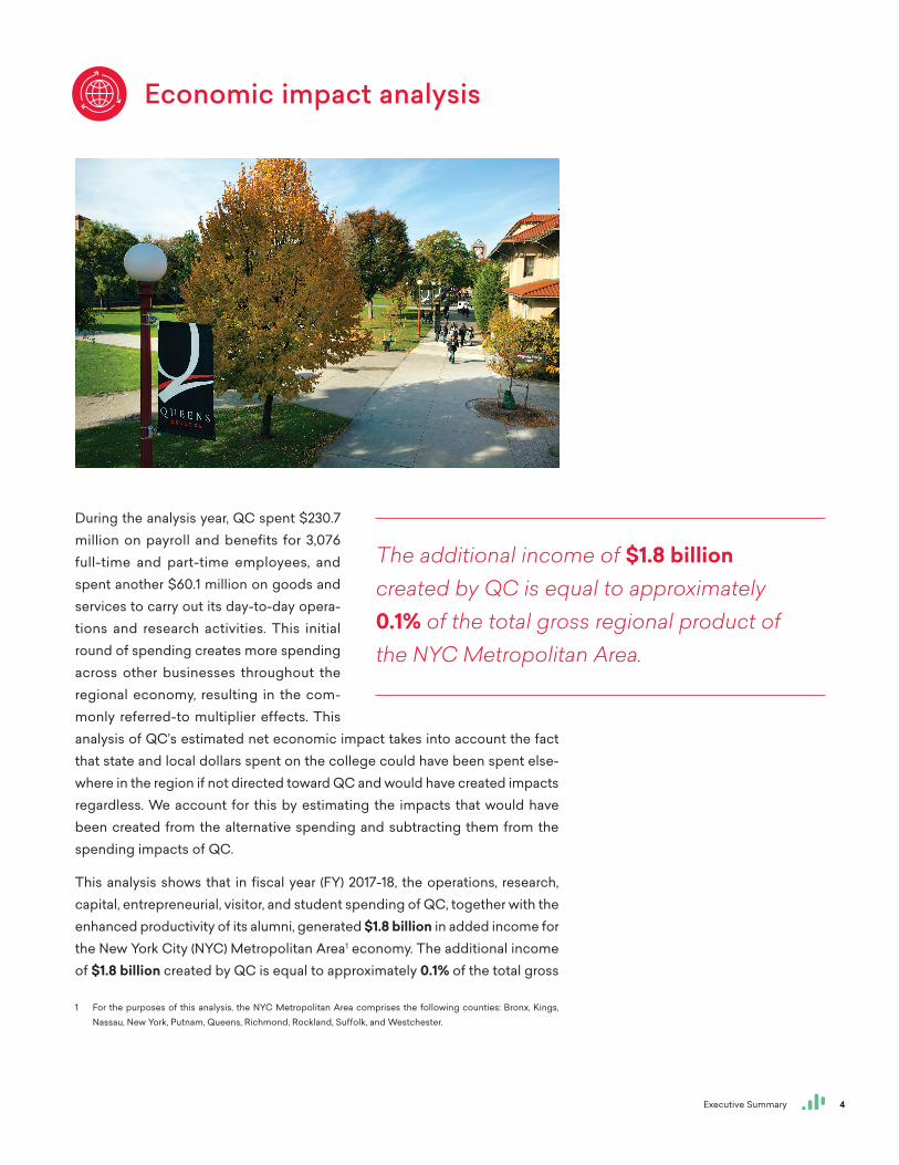
During the analysis year, QC spent $230.7 million on payroll and benefits for 3,076 full-time and part-time employees, and spent another $60.1 million on goods and services to carry out its day-to-day opera-tions and research activities. This initial round of spending creates more spending across other businesses throughout the regional economy, resulting in the com-monly referred-to multiplier effects. This analysis of QC’s estimated net economic impact takes into account the fact that state and local dollars spent on the college could have been spent else-where in the region if not directed toward QC and would have created impacts regardless. We account for this by estimating the impacts that would have been created from the alternative spending and subtracting them from the spending impacts of QC.
This analysis shows that in fiscal year (FY) 2017-18, the operations, research, capital, entrepreneurial, visitor, and student spending of QC, together with the enhanced productivity of its alumni, generated $1.8 billion in added income for the New York City (NYC) Metropolitan Area1 economy. The additional income of $1.8 billion created by QC is equal to approximately 0.1% of the total gross
1 For the purposes of this analysis, the NYC Metropolitan Area comprises the following counties: Bronx, Kings, Nassau, New York, Putnam, Queens, Richmond, Rockland, Suffolk, and Westchester.
The additional income of $1.8 billion created by QC is equal to approximately 0.1% of the total gross regional product of the NYC Metropolitan Area.
5Executive Summary
regional product (GRP) of the NYC Metropolitan Area. This annual impact of $1.8 billion is equivalent to supporting 16,862 jobs. These economic impacts break down as follows:
Operations spending impact
Payroll and benefits to support QC’s day-to-day operations (excluding payroll from research employees) amounted to $223.4 million. The college’s non-pay expenditures amounted to $50.7 million. The net
impact of operations spending by the college in the NYC Metropolitan Area during the analysis year was approximately $276.1 million in added income, which is equivalent to supporting 3,402 jobs.
Research spending impact
QC’s research activities affect the regional economy by employing people and requiring the purchases of equipment, supplies, and services. They also facilitate new knowledge creation throughout the
NYC Metropolitan Area. In FY 2017-18, QC spent $7.3 million on payroll and $9.4 million on other expenditures to support research activities. Research spending of QC generated $11 million in added income for the NYC Metropolitan Area economy, which is equivalent to supporting 131 jobs.
QC faculty and staff impact
QC students learn from leaders in their fields, among them Fulbright fellows, Guggenheim Award recipients, and grantees of the National Institutes of Health. The impact of QC’s renowned faculty and staff
can’t be quantified purely in dollars; however, in economic terms, of the $287.0 million in added income from the operations spending and the research spend-ing impacts to the NYC Metropolitan Area in FY 2017-18, $275.7 million2 is from QC faculty and staff alone. Attracting and retaining researchers, professors, and many professionals to the NYC Metropolitan Area keeps payroll dollars in the region as much of it is spent on goods and services, generating additional economic activity.
Capital spending impact
QC invests in capital each year to maintain its facilities, create additional capacities, and meet its growing educational demands. During FY 2017-18, QC spent a total of $8.5 million of the projected
$189.3 million allocated to the various construction projects. While the amount varies from year to year, these quick infusions of income and jobs have a sub-stantial impact on the regional economy. In FY 2017-18, QC’s capital spending generated $3 million in added income, which is equivalent to supporting 37 jobs.
2 This impact is included within the operations and the research spending impacts and thus should not be summed.
Important note
When reviewing the impacts estimated in this study, it’s important to note that it reports impacts in the form of added income rather than sales. Sales includes all of the intermediary costs associated with producing goods and services, as well as money that leaks out of the region as it is spent at out-of-region businesses. Income, on the other hand, is a net measure that excludes these intermediary costs and leakages, and is synonymous with gross regional product (GRP) and value added. For this reason, it is a more meaningful measure of new economic activity than sales.
6Executive Summary
Start-up and spin-off company impact
QC creates an exceptional environment that fosters innovation and entrepreneurship, evidenced by the number of start-up and spin-off companies related to QC in the region. In FY 2017-18, start-up
and spin-off companies related to QC added $35.8 million in income for the NYC Metropolitan Area economy, which is equivalent to supporting 129 jobs.
Visitor spending impact
Out-of-region visitors attracted to the NYC Metropolitan Area for activities at QC brought new dollars to the economy through their spending at hotels, restaurants, gas stations, and other regional
businesses. The spending from these visitors added approximately $1.8 million in income for the NYC Metropolitan Area economy, which is equivalent to sup-porting 19 jobs during FY 2017-18.
Student spending impact
QC fulfills its mission of serving the community, with its enrollment primarily comprising NYC Metropolitan Area residents. In FY 1718, QC served 829 credit students originating from outside the service
region. These students relocated to the NYC Metropolitan Area to attend the college. In addition, a portion of QC students, referred to as retained students, would have left the NYC Metropolitan Area if not for the existence of QC. The money that these students spent toward living expenses in the NYC Metro-politan Area is attributable to QC.
The expenditures of relocated and retained students in the region during the analysis year added approximately $23.1 million in income for the NYC Metro-politan Area economy, which is equivalent to supporting 301 jobs.
Alumni impact
QC fulfills its mission by primarily serving in-region students. Nearly 70% of all students are from the Borough of Queens. Over the years, students gained new skills, making them more productive workers,
by studying at QC. Today, thousands of these former students are employed in the NYC Metropolitan Area, with nearly 85% of graduates staying in the region and contributing to its brain gain.
The accumulated impact of former students employed in the NYC Met-ropolitan Area workforce amounted to an annual impact of $1.5 billion in added income for the NYC Metropolitan Area economy, which is equivalent to supporting 12,843 jobs.
7Executive Summary
Investment analysis
Investment analysis is the practice of comparing the costs and benefits of an investment to determine whether or not it is profitable. This study considers QC as an investment from the perspectives of students, taxpayers, and society.
Student perspective
Students invest their own money and time in their education to pay for tuition, books, and supplies. Student loans obtained to attend college are included in calculating the cost of attendance. Only
7% of QC students take out loans, with the average amount of a QC student loan in FY 2017-18 at $4,945.3 We account for the loans students will pay back over time. While some students were employed while attending the college, students overall forewent earnings that they would have generated had they been in full employment instead of learning. Summing these direct outlays, opportunity costs, and future student loan costs yields a total of $290.2 million in present value student costs.
In return, students will receive a present value of $1.6 billion in increased earnings over their working lives. This translates to a return of $5.50 in higher future earnings for every dollar that students invest in their education at QC. The corresponding annual rate of return is 17.9%.
3 Tuition cost, financial aid, debt and value evaluation for Queens College (City University of New York) Tuition and Financial Aid, cited by https://www.prepscholar.com/sat/s/colleges/Queens-College-City-University-of-New-York-tuition-financial-aid.
8Executive Summary
Taxpayer perspective
Excluding direct financial aid to students, taxpayers provided $127 million in state and local funding to QC in FY 2017-18. In return, taxpayers will receive an estimated present value of $509.3 million
in added tax revenue stemming from the students’ higher lifetime earnings and the increased output of businesses. Savings to the public sector add another estimated $108.6 million in benefits due to a reduced demand for government-funded social services in New York. For every tax dollar spent educating students attending QC, taxpayers will receive an average of $4.90 in return over the course of the students’ working lives. In other words, taxpayers enjoy an annual rate of return of 13.3%.
Social perspective
For every dollar society invests in QC, an average of $9.90 in benefits will accrue to New York over the course of the students’
careers. People in New York invested $517.2 million in QC in FY 2017-18. This includes the college’s expen-ditures, student expenses, and student opportunity costs. In return, the state of New York will receive an estimated present value of $4.9 billion in added state revenue over the course of the students’ working lives. New York will also benefit from an estimated $236.6 million in present value social savings related to reduced crime, lower welfare and unemployment, and increased health and well-being across the state.
Acknowledgments
Emsi gratefully acknowledges the excellent support of the staff at Queens College in making this study possible. Special thanks go to Dr. William A. Tramontano, Interim President, who approved the study, and to Elizabeth Hendrey, Provost and Vice President for Academic Affairs; William Keller, Vice President for Finance and Administration; Cheryl Littman, Dean of Institutional Effectiveness; Meghan Moore-Wilk, Interim Chief of Staff; Jay Hershenson, Vice President for Communications and Marketing and Senior Advisor to the President; Richard Alvarez, Vice President for Enrollment and Student Retention; Laurie Dorf, Vice President for Institutional Advancement; Adam Rockman, Vice President of the Division of Student Affairs; and Jeffrey Rosenstock, Assistant Vice President for External Affairs, who collected much of the data and information requested. Any errors in the report are the responsibility of Emsi and not of any of the above-mentioned individuals.
For every tax dollar spent educating students attending QC, taxpayers will receive an average of $4.90 in return over the course of the students’ working lives.
9Executive Summary
Introduction
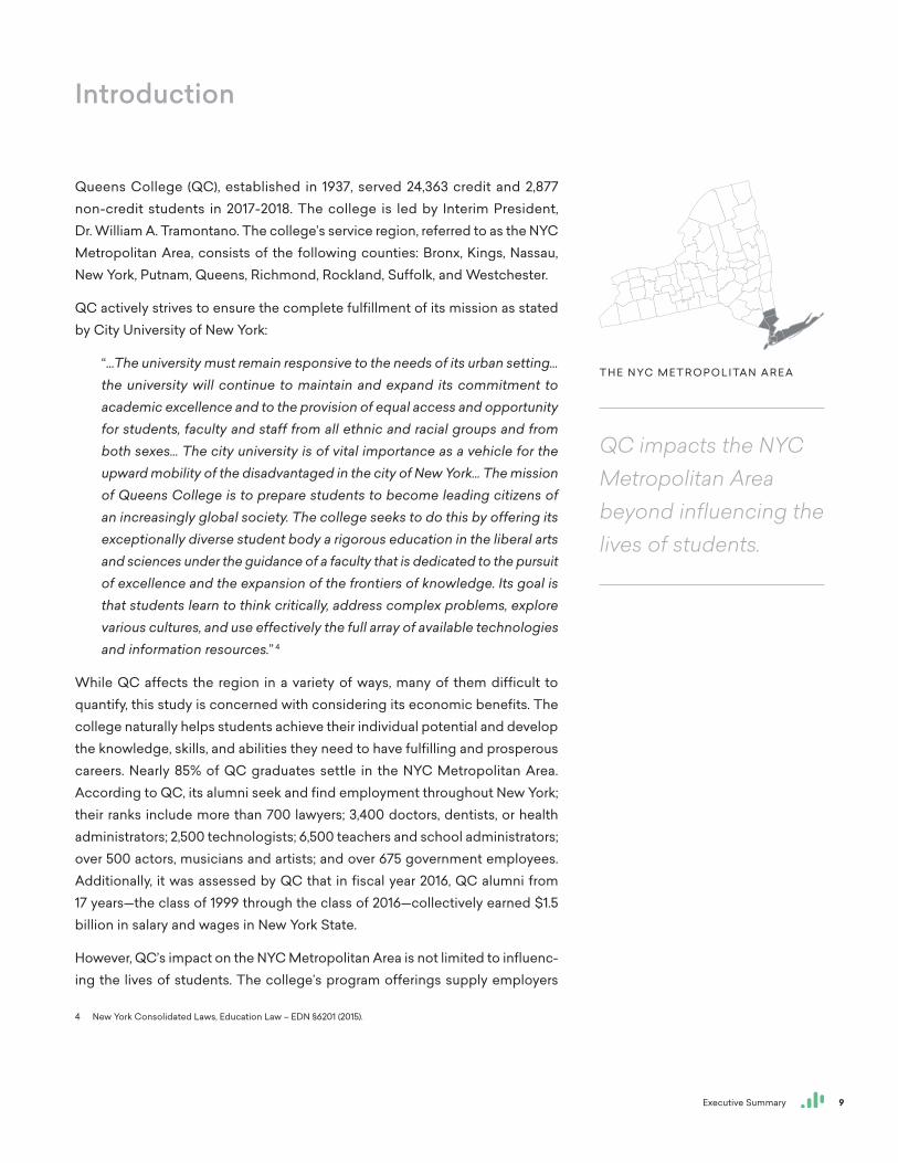
Queens College (QC), established in 1937, served 24,363 credit and 2,877 non-credit students in 2017-2018. The college is led by Interim President, Dr. William A. Tramontano. The college’s service region, referred to as the NYC Metropolitan Area, consists of the following counties: Bronx, Kings, Nassau, New York, Putnam, Queens, Richmond, Rockland, Suffolk, and Westchester.
QC actively strives to ensure the complete fulfillment of its mission as stated by City University of New York:
“…The university must remain responsive to the needs of its urban setting…the university will continue to maintain and expand its commitment to academic excellence and to the provision of equal access and opportunity for students, faculty and staff from all ethnic and racial groups and from both sexes… The city university is of vital importance as a vehicle for the upward mobility of the disadvantaged in the city of New York… The mission of Queens College is to prepare students to become leading citizens of an increasingly global society. The college seeks to do this by offering its exceptionally diverse student body a rigorous education in the liberal arts and sciences under the guidance of a faculty that is dedicated to the pursuit of excellence and the expansion of the frontiers of knowledge. Its goal is that students learn to think critically, address complex problems, explore various cultures, and use effectively the full array of available technologies and information resources.” 4
While QC affects the region in a variety of ways, many of them difficult to quantify, this study is concerned with considering its economic benefits. The college naturally helps students achieve their individual potential and develop the knowledge, skills, and abilities they need to have fulfilling and prosperous careers. Nearly 85% of QC graduates settle in the NYC Metropolitan Area. According to QC, its alumni seek and find employment throughout New York; their ranks include more than 700 lawyers; 3,400 doctors, dentists, or health administrators; 2,500 technologists; 6,500 teachers and school administrators; over 500 actors, musicians and artists; and over 675 government employees. Additionally, it was assessed by QC that in fiscal year 2016, QC alumni from 17 years—the class of 1999 through the class of 2016—collectively earned $1.5 billion in salary and wages in New York State.
However, QC’s impact on the NYC Metropolitan Area is not limited to influenc-ing the lives of students. The college’s program offerings supply employers
4 New York Consolidated Laws, Education Law – EDN §6201 (2015).
QC impacts the NYC Metropolitan Area beyond influencing the lives of students.
T H E N YC M E T R O P O L I TA N A R E A
10Executive Summary
with workers to make their businesses more productive. Furthermore, QC is committed to promoting supplier diversity and to ensuring that NYS-certified minority- and women-owned business enterprises (MWBE) are provided an equal opportunity to offer the college goods and services at competitive prices. According to QC, MWBE participation in 2018 was 36%, based on actual QC MWBE spending of $1.1 million.
The college, its day-to-day and research operations, its construction and entrepreneurial activities, and the expenditures of its visitors and students support the regional economy through the output and employment gener-ated by regional vendors. The benefits created by the college extend as far as the state treasury in terms of the increased tax receipts and decreased public sector costs generated by students across the state.
This report assesses the impact of QC as a whole on the regional economy and the benefits generated by the college for students, taxpayers, and society. The approach is twofold. We begin with an economic impact analysis of the college on the NYC Metropolitan Area economy. To derive results, we rely on a specialized Multi-Regional Social Accounting Matrix (MR-SAM) model to calculate the added income created in the NYC Metropolitan Area economy as a result of increased consumer spending and the added knowledge, skills, and abilities of students. Results of the economic impact analysis are broken out according to the following impacts: 1) impact of the college’s day-to-day operations, 2) impact of its research spending, 3) impact of its capital spending, 4) impact of entrepreneurial activities, 5) impact of visitor spending, 6) impact of student spending, and 7) impact of alumni who are still employed in the NYC Metropolitan Area workforce.
The second component of the study measures the benefits generated by QC for the following stakeholder groups: students, taxpayers, and society. For stu-dents, we perform an investment analysis to determine how the money spent by students on their education performs as an investment over time. The students’ investment in this case consists of their out-of-pocket expenses, the cost of interest incurred on student loans, and the opportunity cost of attending the college as opposed to working. In return for these investments, students receive a lifetime of higher earnings. For taxpayers, the study measures the benefits to state taxpayers in the form of increased tax revenues and public sector savings stemming from a reduced demand for social services. Finally, for society, the study assesses how the students’ higher earnings and improved quality of life create benefits throughout New York as a whole.
The study uses a wide array of data based on several sources, including the FY 2017-18 academic and financial reports from QC; industry and employment data from the Bureau of Labor Statistics and Census Bureau; outputs of Emsi’s impact model and MR-SAM model; and published materials relating education to social behavior.
Chapter 1: Profile of Queens College and the Economy 11
C H A P T E R 1 :
Profile of Queens College and the Economy
Queens College (QC), a member of the City University of New York network, is one of New York’s largest and most respected liberal arts colleges, as well as one of the best educational values in America according to the Center on Education and the Workforce.5 Based in New York’s Flushing Neighborhood, QC’s urban campus offers students from every background and part of society the opportunity to pursue a world-class education in New York. During
FY 2017-18, the college had a total enrollment of over 27,000 credit and non-credit students.
5 https://cew.georgetown.edu/about-us/
Chapter 1: Profile of Queens College and the Economy 12
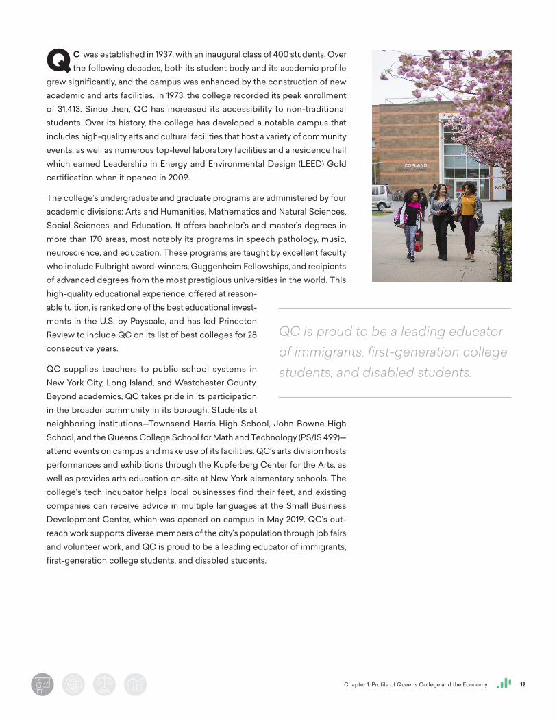
QC was established in 1937, with an inaugural class of 400 students. Over the following decades, both its student body and its academic profile
grew significantly, and the campus was enhanced by the construction of new academic and arts facilities. In 1973, the college recorded its peak enrollment of 31,413. Since then, QC has increased its accessibility to non-traditional students. Over its history, the college has developed a notable campus that includes high-quality arts and cultural facilities that host a variety of community events, as well as numerous top-level laboratory facilities and a residence hall which earned Leadership in Energy and Environmental Design (LEED) Gold certification when it opened in 2009.
The college’s undergraduate and graduate programs are administered by four academic divisions: Arts and Humanities, Mathematics and Natural Sciences, Social Sciences, and Education. It offers bachelor’s and master’s degrees in more than 170 areas, most notably its programs in speech pathology, music, neuroscience, and education. These programs are taught by excellent faculty who include Fulbright award-winners, Guggenheim Fellowships, and recipients of advanced degrees from the most prestigious universities in the world. This high-quality educational experience, offered at reason-able tuition, is ranked one of the best educational invest-ments in the U.S. by Payscale, and has led Princeton Review to include QC on its list of best colleges for 28 consecutive years.
QC supplies teachers to public school systems in New York City, Long Island, and Westchester County. Beyond academics, QC takes pride in its participation in the broader community in its borough. Students at neighboring institutions—Townsend Harris High School, John Bowne High School, and the Queens College School for Math and Technology (PS/IS 499)—attend events on campus and make use of its facilities. QC’s arts division hosts performances and exhibitions through the Kupferberg Center for the Arts, as well as provides arts education on-site at New York elementary schools. The college’s tech incubator helps local businesses find their feet, and existing companies can receive advice in multiple languages at the Small Business Development Center, which was opened on campus in May 2019. QC’s out-reach work supports diverse members of the city’s population through job fairs and volunteer work, and QC is proud to be a leading educator of immigrants, first-generation college students, and disabled students.
QC is proud to be a leading educator of immigrants, first-generation college students, and disabled students.
Chapter 1: Profile of Queens College and the Economy 13
QC employee and finance data
The study uses two general types of information: 1) data collected from the college and 2) regional economic data obtained from various public sources and Emsi’s proprietary data modeling tools.6 This chapter presents the basic underlying information from QC used in this analysis and provides an overview of the NYC Metropolitan Area economy.
Employee data
Data provided by QC include information on faculty and staff by place of work and by place of residence. These data appear in Table 1.1. As shown, QC employed 1,373 full-time and 1,703 part-time faculty and staff in FY 2017-18 (including student workers). All QC employees worked in the region and 95% resided in the region. These data are used to isolate the portion of the employ-ees’ payroll and household expenses that remains in the regional economy.
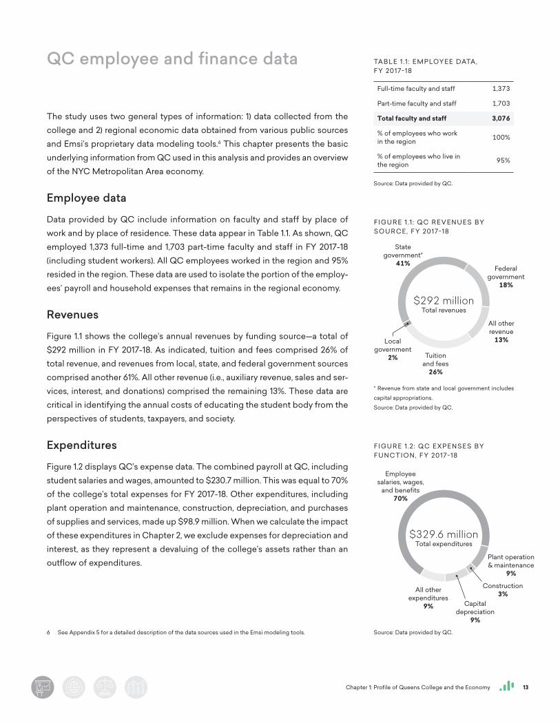
Revenues
Figure 1.1 shows the college’s annual revenues by funding source—a total of $292 million in FY 2017-18. As indicated, tuition and fees comprised 26% of total revenue, and revenues from local, state, and federal government sources comprised another 61%. All other revenue (i.e., auxiliary revenue, sales and ser-vices, interest, and donations) comprised the remaining 13%. These data are critical in identifying the annual costs of educating the student body from the perspectives of students, taxpayers, and society.
Expenditures
Figure 1.2 displays QC’s expense data. The combined payroll at QC, including student salaries and wages, amounted to $230.7 million. This was equal to 70% of the college’s total expenses for FY 2017-18. Other expenditures, including plant operation and maintenance, construction, depreciation, and purchases of supplies and services, made up $98.9 million. When we calculate the impact of these expenditures in Chapter 2, we exclude expenses for depreciation and interest, as they represent a devaluing of the college’s assets rather than an outflow of expenditures.
6 See Appendix 5 for a detailed description of the data sources used in the Emsi modeling tools.
TA B L E 1 .1 : E M P LOY E E DATA, F Y 2017-18
Full-time faculty and staff 1,373
Part-time faculty and staff 1,703
Total faculty and staff 3,076
% of employees who work in the region 100%
% of employees who live in the region 95%
Source: Data provided by QC.
F I G U R E 1 .1 : Q C R E V E N U E S BY S O U R C E, F Y 2017-18
* Revenue from state and local government includes
capital appropriations.
Source: Data provided by QC.
1818+1313+2626+22+4141+R$292 millionTotal revenues
Tuition and fees
26%
State government*
41%
Local government
2%
Federal government
18%
All other revenue
13%
F I G U R E 1 .2 : Q C E X P E N S E S BY F U N C T I O N, F Y 2017-1899
+33+99+99+7070+R $329.6 millionTotal expenditures
Employee salaries, wages,
and benefits70%
Plant operation & maintenance
9%
Capital depreciation
9%
Construction3%All other
expenditures9%
Source: Data provided by QC.
Chapter 1: Profile of Queens College and the Economy 14
Students
QC served 24,363 students taking courses for credit and 2,877 non-credit students in FY 2017-18. These numbers represent unduplicated student head-counts. The breakdown of the student body by gender was 57% female and 43% male. The breakdown by ethnicity was 70% students of color and 30% white. The students’ average age was 24 years old.7 An estimated 83% of students remain in the NYC Metropolitan Area after finishing their time at QC, another 4% settle outside the region but within the state, and the remaining 13% settle outside the state.8
Table 1.2 summarizes the breakdown of the student population and its corre-sponding awards and credits by education level. In FY 2017-18, QC served 881 master’s degree graduates, 266 post-bachelor’s certificate graduates, and 2,367 bachelor’s degree graduates. Another 19,799 students enrolled in courses for credit but did not complete a degree during the reporting year. The college offered dual-credit courses to high schools, serving a total of 1,042 students over the course of the year. The college also served eight personal enrichment stu-dents enrolled in non-credit courses. Non-degree seeking students enrolled in workforce or professional development programs accounted for 2,877 students.
We use credit hour equivalents (CHEs) to track the educational workload of the students. One CHE is equal to 15 contact hours of classroom instruction per semester. In the analysis, we exclude the CHE production of personal enrich-ment students under the assumption that they do not attain knowledge, skills, and abilities that will increase their earnings. The average number of CHEs per student (excluding personal enrichment students) was 15.2 for the academic year.
7 Unduplicated headcount, gender, ethnicity, and age data provided by QC.8 Settlement data provided by QC.
TA B L E 1 .2 : B R E A K D OW N O F S T U D E N T H E A D C O U N T A N D C H E P R O D U C T I O N BY E D U CAT I O N L E V E L, F Y 2017-18
Category Headcount Total CHEs Average CHEs
Master’s degree graduates 881 11,006 12.5
Post-bachelor’s certificate completers 266 3,214 12.1
Bachelor’s degree graduates 2,367 47,330 20.0
Continuing students 19,799 344,751 17.4
Dual credit students 1,042 7,149 6.9
Personal enrichment students 8 32 4.0
Workforce/professional development students 2,877 289 0.1
Total, all students 27,240 413,771 15.2
Total, less personal enrichment students 27,232 413,739 15.2
Source: Data provided by QC.
Chapter 1: Profile of Queens College and the Economy 15
The NYC Metropolitan Area economy
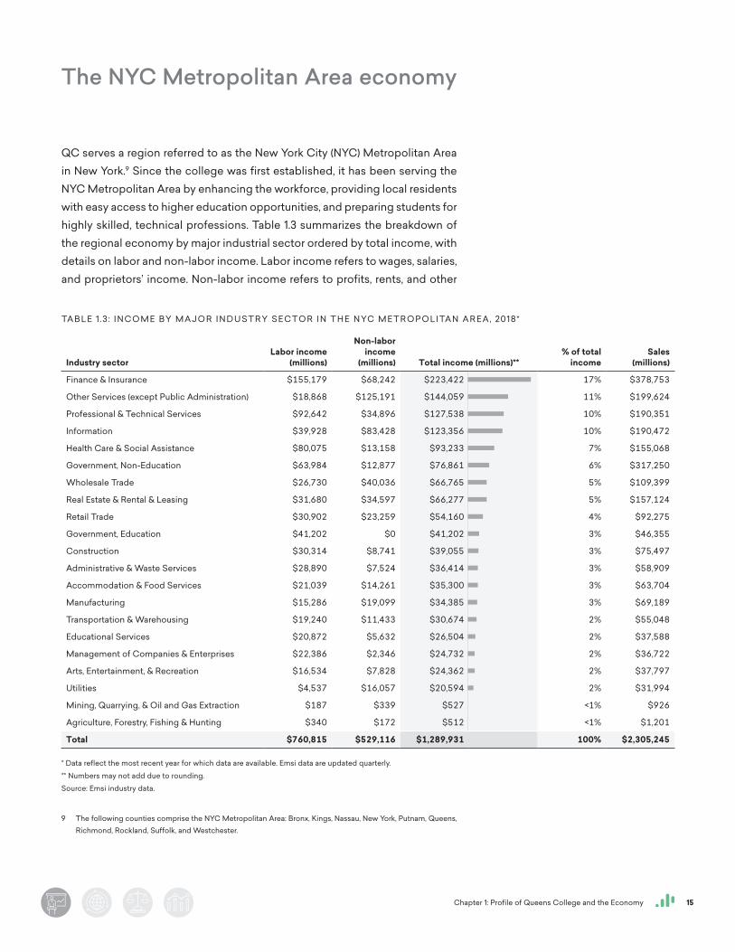
QC serves a region referred to as the New York City (NYC) Metropolitan Area in New York.9 Since the college was first established, it has been serving the NYC Metropolitan Area by enhancing the workforce, providing local residents with easy access to higher education opportunities, and preparing students for highly skilled, technical professions. Table 1.3 summarizes the breakdown of the regional economy by major industrial sector ordered by total income, with details on labor and non-labor income. Labor income refers to wages, salaries, and proprietors’ income. Non-labor income refers to profits, rents, and other
9 The following counties comprise the NYC Metropolitan Area: Bronx, Kings, Nassau, New York, Putnam, Queens, Richmond, Rockland, Suffolk, and Westchester.
TA B L E 1 .3 : I N C O M E BY M A J O R I N D U S T R Y S E C TO R I N T H E N YC M E T R O P O L I TA N A R E A, 2018*
Industry sectorLabor income
(millions)
Non-labor income
(millions) Total income (millions)**% of total
incomeSales
(millions)
Finance & Insurance $155,179 $68,242 $223,422 17% $378,753
Other Services (except Public Administration) $18,868 $125,191 $144,059 11% $199,624
Professional & Technical Services $92,642 $34,896 $127,538 10% $190,351
Information $39,928 $83,428 $123,356 10% $190,472
Health Care & Social Assistance $80,075 $13,158 $93,233 7% $155,068
Government, Non-Education $63,984 $12,877 $76,861 6% $317,250
Wholesale Trade $26,730 $40,036 $66,765 5% $109,399
Real Estate & Rental & Leasing $31,680 $34,597 $66,277 5% $157,124
Retail Trade $30,902 $23,259 $54,160 4% $92,275
Government, Education $41,202 $0 $41,202 3% $46,355
Construction $30,314 $8,741 $39,055 3% $75,497
Administrative & Waste Services $28,890 $7,524 $36,414 3% $58,909
Accommodation & Food Services $21,039 $14,261 $35,300 3% $63,704
Manufacturing $15,286 $19,099 $34,385 3% $69,189
Transportation & Warehousing $19,240 $11,433 $30,674 2% $55,048
Educational Services $20,872 $5,632 $26,504 2% $37,588
Management of Companies & Enterprises $22,386 $2,346 $24,732 2% $36,722
Arts, Entertainment, & Recreation $16,534 $7,828 $24,362 2% $37,797
Utilities $4,537 $16,057 $20,594 2% $31,994
Mining, Quarrying, & Oil and Gas Extraction $187 $339 $527 <1% $926
Agriculture, Forestry, Fishing & Hunting $340 $172 $512 <1% $1,201
Total $760,815 $529,116 $1,289,931 100% $2,305,245
* Data reflect the most recent year for which data are available. Emsi data are updated quarterly.
** Numbers may not add due to rounding.
Source: Emsi industry data.
100+64+57+55+42+34+30+30+24+18+17+16+16+15+14+12+11+11+9+0+0
Chapter 1: Profile of Queens College and the Economy 16
forms of investment income. Together, labor and non-labor income comprise the region’s total income, which can also be considered the region’s gross regional product (GRP).
As shown in Table 1.3, the total income, or GRP, of the NYC Metropolitan Area is approximately $1.3 trillion, equal to the sum of labor income ($760.8 billion) and non-labor income ($529.1 billion). In Chapter 2, we use the total added income as the measure of the relative impacts of the college on the regional economy.
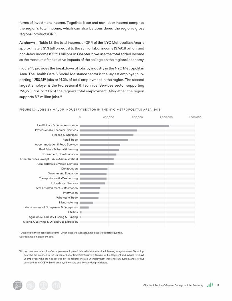
Figure 1.3 provides the breakdown of jobs by industry in the NYC Metropolitan Area. The Health Care & Social Assistance sector is the largest employer, sup-porting 1,250,319 jobs or 14.3% of total employment in the region. The second largest employer is the Professional & Technical Services sector, supporting 795,228 jobs or 9.1% of the region’s total employment. Altogether, the region supports 8.7 million jobs.10
10 Job numbers reflect Emsi’s complete employment data, which includes the following four job classes: 1) employ-ees who are counted in the Bureau of Labor Statistics’ Quarterly Census of Employment and Wages (QCEW), 2) employees who are not covered by the federal or state unemployment insurance (UI) system and are thus excluded from QCEW, 3) self-employed workers, and 4) extended proprietors.
F I G U R E 1 .3 : J O B S BY M A J O R I N D U S T R Y S E C TO R I N T H E N YC M E T R O P O L I TA N A R E A, 2018*
Health Care & Social Assistance
Professional & Technical Services
Finance & Insurance
Retail Trade
Accommodation & Food Services
Real Estate & Rental & Leasing
Government, Non-Education
Other Services (except Public Administration)
Administrative & Waste Services
Construction
Government, Education
Transportation & Warehousing
Educational Services
Arts, Entertainment, & Recreation
Information
Wholesale Trade
Manufacturing
Management of Companies & Enterprises
Utilities
Agriculture, Forestry, Fishing & Hunting
Mining, Quarrying, & Oil and Gas Extraction
* Data reflect the most recent year for which data are available. Emsi data are updated quarterly.
Source: Emsi employment data.
100+100+100+100+100+100+100+100+100+100+100+100+100+100+100+100+100+100+100+100+1001,600,0001,200,000800,0000 400,000100+64+60+54+45+44+41+38+38+31+30+30+28+23+22+21+15+10+2+1+0
Chapter 1: Profile of Queens College and the Economy 17
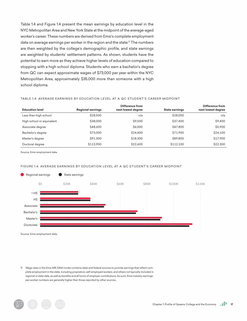
Table 1.4 and Figure 1.4 present the mean earnings by education level in the NYC Metropolitan Area and New York State at the midpoint of the average-aged worker’s career. These numbers are derived from Emsi’s complete employment data on average earnings per worker in the region and the state.11 The numbers are then weighted by the college’s demographic profile, and state earnings are weighted by students’ settlement patterns. As shown, students have the potential to earn more as they achieve higher levels of education compared to stopping with a high school diploma. Students who earn a bachelor’s degree from QC can expect approximate wages of $73,000 per year within the NYC Metropolitan Area, approximately $35,000 more than someone with a high school diploma.
11 Wage rates in the Emsi MR-SAM model combine state and federal sources to provide earnings that reflect com-plete employment in the state, including proprietors, self-employed workers, and others not typically included in regional or state data, as well as benefits and all forms of employer contributions. As such, Emsi industry earnings-per-worker numbers are generally higher than those reported by other sources.
TA B L E 1 .4 : AV E R AG E E A R N I N G S BY E D U CAT I O N L E V E L AT A Q C S T U D E N T’ S CA R E E R M I D P O I N T
Education level Regional earningsDifference from
next lowest degree State earningsDifference from
next lowest degree
Less than high school $28,500 n/a $28,000 n/a
High school or equivalent $38,000 $9,500 $37,400 $9,400
Associate degree $48,600 $6,000 $47,800 $5,900
Bachelor’s degree $73,000 $24,400 $71,900 $24,100
Master’s degree $91,300 $18,300 $89,800 $17,900
Doctoral degree $113,900 $22,600 $112,100 $22,300
Source: Emsi employment data.
F I G U R E 1 .4 : AV E R AG E E A R N I N G S BY E D U CAT I O N L E V E L AT A Q C S T U D E N T’ S CA R E E R M I D P O I N T
Source: Emsi employment data.
< HS
HS
Associate
Bachelor's
Master's
Doctorate
Regional earnings State earnings
$120K$80K$60K$40K$0 $20K $100K25+33+43+64+80+10025+33+42+63+79+98
Chapter 2: Economic Impacts on the NYC Metropolitan Area Economy 18
C H A P T E R 2 :
Economic Impacts on the NYC Metropolitan Area Economy
QC affects the NYC Metropolitan Area economy in a variety of ways. The college is an employer and buyer of goods and services. It attracts monies that otherwise would not
have entered the regional economy through its day-to-day and research operations, its construction and entrepreneurial activities, and the expenditures of its visitors and
students. Further, it provides students with the knowledge, skills, and abilities they need to become productive citizens and add to the region’s overall output.
Chapter 2: Economic Impacts on the NYC Metropolitan Area Economy 19
IN this chapter, we estimate the following economic impacts of QC: 1) the operations spending impact, 2) the research spending impact, 3) the capital
spending impact, 4) the start-up and spin-off company impact, 5) the visitor spending impact, 6) the student spending impact, and 7) the alumni impact, measuring the income added in the region as former students expand the regional economy’s stock of human capital.
When exploring each of these economic impacts, we consider the following hypothetical question:
How would economic activity change in the NYC Metropolitan Area if QC and all its alumni did not exist in FY 2017-18?
Each of the economic impacts should be interpreted according to this hypotheti-cal question. Another way to think about the question is to realize that we mea-sure net impacts, not gross impacts. Gross impacts represent an upper-bound estimate in terms of capturing all activity stemming from the college; however, net impacts reflect a truer measure of economic impact since they demonstrate what would not have existed in the regional economy if not for the college.
Economic impact analyses use different types of impacts to estimate the results. The impact focused on in this study assesses the change in income. This measure is similar to the commonly used gross regional product (GRP). Income may be further broken out into the labor income impact, also known as earnings, which assesses the change in employee compensation; and the non-labor income impact, which assesses the change in business profits. Together, labor income and non-labor income sum to total income.
Another way to state the impact is in terms of jobs, a measure of the number of full- and part-time positions that would be required to support the change in income. Finally, a frequently used measure is the sales impact, which comprises the change in business sales revenue in the economy as a result of increased economic activity. It is important to bear in mind, however, that much of this sales revenue leaves the regional economy through intermediary transactions and costs.12 All of these measures—added labor and non-labor income, total income, jobs, and sales—are used to estimate the economic impact results presented in this chapter. The analysis breaks out the impact measures into different components, each based on the economic effect that caused the impact. The following is a list of each type of effect presented in this analysis:
• The initial effect is the exogenous shock to the economy caused by the initial spending of money, whether to pay for salaries and wages, purchase goods or services, or cover operating expenses.
• The initial round of spending creates more spending in the economy, resulting in what is commonly known as the multiplier effect. The multiplier
12 See Appendix 4 for an example of the intermediary costs included in the sales impact but not in the income impact.
Operations Spending Impact
TOTAL ECONOMIC IMPACT
Capital Spending Impact
Start-up & Spin-off Company Impact
Research Spending Impact
Student Spending Impact
Visitor Spending Impact
Alumni Impact
Chapter 2: Economic Impacts on the NYC Metropolitan Area Economy 20
effect comprises the additional activity that occurs across all industries in the economy and may be further decomposed into the following three types of effects:
· The direct effect refers to the additional economic activity that occurs as the initially affected industries spend money to purchase goods and services from their supply chain industries.
· The indirect effect occurs as the supply chain of the initial industries creates even more activity in the economy through inter-industry spending.
· The induced effect refers to the economic activ-ity created by the household sector as the initially, directly, and indirectly affected businesses raise sala-ries or hire more people.
The terminology used to describe the economic effects listed above dif-fers slightly from that of other commonly used input-output models, such as IMPLAN. For example, the initial effect in this study is called the “direct effect” by IMPLAN, as shown in the table below. Further, the term “indirect effect” as used by IMPLAN refers to the combined direct and indirect effects defined in this study. To avoid confusion, readers are encouraged to interpret the results presented in this chapter in the context of the terms and definitions listed above. Note that, regardless of the effects used to decompose the results, the total impact measures are analogous.
Multiplier effects in this analysis are derived using Emsi’s Multi-Regional Social Accounting Matrix (MR-SAM) input-output model, which captures the inter-connection of industries, government, and households in the region. The Emsi MR-SAM contains approximately 1,000 industry sectors at the highest level of detail available in the North American Industry Classification System (NAICS) and supplies the industry-specific multipliers required to determine the impacts associated with increased activity within a given economy. The multi-regional capacity of the MR-SAM allows impacts to be measured in the region and state simultaneously, taking into account QC’s activity in each area, as well as each area’s economic characteristics. In this analysis, impacts on the region include impacts from the college’s regional activity, as well as the indirect and induced multiplier effects that reach the region from the college’s activity in the rest of the state. For more information on the Emsi MR-SAM model and its data sources, see Appendix 5.
Net impacts reflect a truer measure of economic impact since they demonstrate what would not have existed in the regional economy if not for the college.
Emsi Initial Direct Indirect Induced
IMPLAN Direct Indirect Induced
Chapter 2: Economic Impacts on the NYC Metropolitan Area Economy 21
Operations spending impact
Faculty and staff payroll is part of the region’s total earnings, and the spend-ing of employees for groceries, apparel, and other household expenditures helps support regional businesses. The college itself purchases supplies and services, and many of its vendors are located in the NYC Metropolitan Area. These expenditures create a ripple effect that generates still more jobs and higher wages throughout the economy.
Table 2.1 presents college expenditures (excluding research and capital spend-ing) for the following three categories: 1) salaries, wages, and benefits, 2) opera-tion and maintenance of plant, and 3) all other expenditures (including purchases
QC’s facilities serve as resources to the community
The college’s considerable athletic facilities—including an aquatics center, a fitness center, and a tennis cen-ter—are open at favorable rates to members of the general public. QC’s athletics department runs a summer camp that serves local children, offering academic enrichment, theatrical workshops, computer training, and of course, sports. Local high schools make use of QC’s fields as well as our outdoor track, where it’s common to see neighborhood residents of all ages walking and jogging.
THE KUPFERBERG CENTER FOR THE ARTS
The Kupferberg Center for the Arts is the borough’s top arts destination, attracting audiences from all over the city as well as Long Island. Kupferberg’s extraordinary calendar of events encompasses music, theater, and dance performances, readings by celebrated writers, and exhibitions drawing on the holdings of the Godwin-Ternbach Museum, a teaching institution with a collection of over 6,000 objects from antiquity to the present. (Admission to the Godwin-Ternbach and other galleries on campus is always free.)
Many schoolchildren see their first art show, concert, or play on this campus. But they don’t have to come to campus to have their horizons expanded. Through the Bach to School program, advanced music students from the Aaron Copland School of Music perform chamber music at elementary schools.
Kupferberg facilities include the Louis Armstrong House Museum (LAHM), furnished as it was when Satchmo lived there. Jazz aficionados and researchers from all over the world make pilgrimages to LAHM to learn more about its namesake and listen to performers building on his legacy.
SPEECH-LANGUAGE HEARING CENTER
Since 1942, the QC Speech-Language Hearing Center has treated children and adults in the Queens com-munity who have speech and language disorders that impact their ability to communicate. Over 250 assess-ment and treatment sessions are provided each year to persons from age 16 months to 99 years old with a variety of communication disorders. The Center also houses the highly regarded and nationally accredited, graduate program in speech-language pathology, with 350 highly trained and diverse students graduated from the program during the last few years. Our students have been highly successful in pursuing additional graduate studies and careers in speech-language pathology or audiology. Many have leadership positions in Queens at hospitals, rehabilitation centers, schools, home care, pre-schools and specialty practices.
Chapter 2: Economic Impacts on the NYC Metropolitan Area Economy 22
for supplies and services). In this analysis, we exclude expenses for deprecia-tion and interest due to the way those measures are calculated in the national input-output accounts, and because depreciation represents the devaluing of the college’s assets rather than an outflow of expenditures.13 The first step in estimating the multiplier effects of the college’s operational expenditures is to map these categories of expenditures to the approximately 1,000 industries of the Emsi MR-SAM model. Assuming that the spending patterns of college personnel approximately match those of the average consumer, we map salaries, wages, and benefits to spending on industry outputs using national household expenditure coefficients provided by Emsi’s national SAM. All QC employees work in the NYC Metropolitan Area (see Table 1.1), and therefore we consider 100% of the salaries, wages, and benefits. For the other two expenditure cat-egories (i.e., operation and maintenance of plant and all other expenditures), we assume the college’s spending patterns approximately match national aver-ages and apply the national spending coefficients for NAICS 902612 (Colleges, Universities, and Professional Schools (State Government)).14 Operation and maintenance of plant expenditures are mapped to the industries that relate to capital construction, maintenance, and support, while the college’s remaining expenditures are mapped to the remaining industries.
We now have three vectors of expenditures for QC: one for salaries, wages, and benefits; another for plant operation and maintenance; and a third for the college’s purchases of supplies and services. The next step is to estimate the portion of these expenditures that occur inside the region. The expenditures occurring outside the region are known as leakages. We estimate in-region expenditures using regional purchase coefficients (RPCs), a measure of the overall demand for the commodities produced by each sector that is satisfied by regional suppliers, for each of the approximately 1,000 industries in the
13 This aligns with the economic impact guidelines set by the Association of Public and Land-Grant Universities. Ultimately, excluding these measures results in more conservative and defensible estimates.
14 See Appendix 2 for a definition of NAICS.
TA B L E 2.1 : Q C E X P E N S E S BY F U N C T I O N ( E XC L U D I N G D E P R E C I AT I O N & I N T E R E S T) , F Y 2017-18
Expense categoryIn-region expenditures
(thousands)Out-of-region expenditures
(thousands)Total expenditures
(thousands)
Employee salaries, wages, and benefits $223,374 $0 $223,374
Plant operation and maintenance $23,273 $6,825 $30,098
All other expenditures $8,302 $12,313 $20,616
Total $254,949 $19,138 $274,088
This table does not include expenditures for research or construction activities, as they are presented separately in the following sections.
Source: Data provided by QC and the Emsi impact model.
Chapter 2: Economic Impacts on the NYC Metropolitan Area Economy 23
MR-SAM model.15 For example, if 40% of the demand for NAICS 541211 (Offices of Certified Public Accountants) is satisfied by regional suppliers, the RPC for that industry is 40%. The remaining 60% of the demand for NAICS 541211 is provided by suppliers located outside the region. The three vectors of expen-ditures are multiplied, industry by industry, by the corresponding RPC to arrive at the in-region expenditures associated with the college. See Table 2.1 for a break-out of the expenditures that occur in-region. Finally, in-region spending is entered, industry by industry, into the MR-SAM model’s multiplier matrix, which in turn provides an estimate of the associated multiplier effects on regional labor income, non-labor income, total income, sales, and jobs.
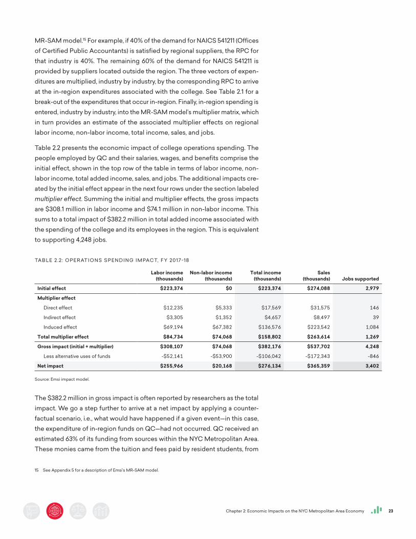
Table 2.2 presents the economic impact of college operations spending. The people employed by QC and their salaries, wages, and benefits comprise the initial effect, shown in the top row of the table in terms of labor income, non-labor income, total added income, sales, and jobs. The additional impacts cre-ated by the initial effect appear in the next four rows under the section labeled multiplier effect. Summing the initial and multiplier effects, the gross impacts are $308.1 million in labor income and $74.1 million in non-labor income. This sums to a total impact of $382.2 million in total added income associated with the spending of the college and its employees in the region. This is equivalent to supporting 4,248 jobs.
The $382.2 million in gross impact is often reported by researchers as the total impact. We go a step further to arrive at a net impact by applying a counter-factual scenario, i.e., what would have happened if a given event—in this case, the expenditure of in-region funds on QC—had not occurred. QC received an estimated 63% of its funding from sources within the NYC Metropolitan Area. These monies came from the tuition and fees paid by resident students, from
15 See Appendix 5 for a description of Emsi’s MR-SAM model.
TA B L E 2.2 : O P E R AT I O N S S P E N D I N G I M PAC T, F Y 2017-18
Labor income
(thousands)Non-labor income
(thousands)Total income
(thousands)Sales
(thousands) Jobs supported
Initial effect $223,374 $0 $223,374 $274,088 2,979
Multiplier effect
Direct effect $12,235 $5,333 $17,569 $31,575 146
Indirect effect $3,305 $1,352 $4,657 $8,497 39
Induced effect $69,194 $67,382 $136,576 $223,542 1,084
Total multiplier effect $84,734 $74,068 $158,802 $263,614 1,269
Gross impact (initial + multiplier) $308,107 $74,068 $382,176 $537,702 4,248
Less alternative uses of funds -$52,141 -$53,900 -$106,042 -$172,343 -846
Net impact $255,966 $20,168 $276,134 $365,359 3,402
Source: Emsi impact model.
Chapter 2: Economic Impacts on the NYC Metropolitan Area Economy 24
the auxiliary revenue and donations from private sources located within the region, from state and local taxes, and from the financial aid issued to students by state and local government. We must account for the opportunity cost of this in-region funding. Had other industries received these monies rather than QC, income impacts would have still been created in the economy. In economic analysis, impacts that occur under counter-factual conditions are used to offset the impacts that actually occur in order to derive the true impact of the event under analysis.
We estimate this counterfactual by simulating a sce-nario where in-region monies spent on the college are instead spent on consumer goods and savings. This simulates the in-region monies being returned to the taxpayers and being spent by the household sector. Our approach is to establish the total amount spent by in-region students and taxpayers on QC, map this to the detailed industries of the MR-SAM model using national household expenditure coefficients, use the industry RPCs to estimate in-region spending, and run the in-region spending through the MR-SAM model’s multiplier matrix to derive multiplier effects. The results of this exercise are shown as negative values in the row labeled less alternative uses of funds in Table 2.2.
The total net impact of the college’s operations is equal to the gross impact minus the impact of the alternative use of funds—the opportunity cost of the regional money. As shown in the last row of Table 2.2, the total net impact is approximately $256 million in labor income and $20.2 million in non-labor income. This sums together to $276.1 million in total added income and is equiv-alent to supporting 3,402 jobs. These impacts represent new economic activity created in the regional economy solely attributable to the operations of QC.
The total net impact of the college’s operations is $276.1 million in total added income, which is equivalent to supporting 3,402 jobs.
Chapter 2: Economic Impacts on the NYC Metropolitan Area Economy 25
Research spending impact
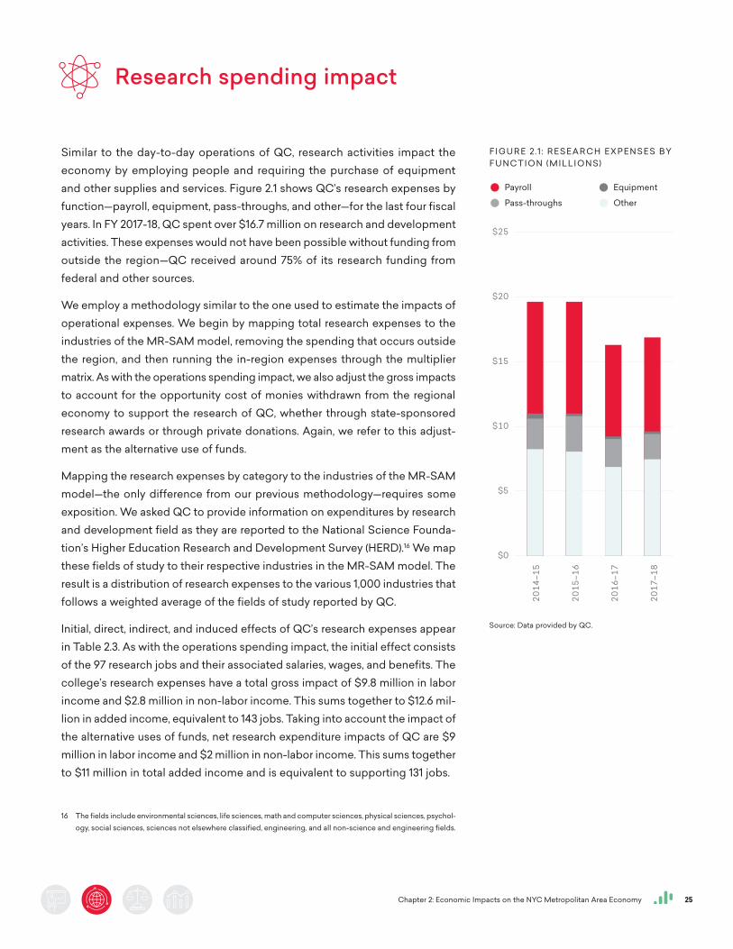
Similar to the day-to-day operations of QC, research activities impact the economy by employing people and requiring the purchase of equipment and other supplies and services. Figure 2.1 shows QC’s research expenses by function—payroll, equipment, pass-throughs, and other—for the last four fiscal years. In FY 2017-18, QC spent over $16.7 million on research and development activities. These expenses would not have been possible without funding from outside the region—QC received around 75% of its research funding from federal and other sources.
We employ a methodology similar to the one used to estimate the impacts of operational expenses. We begin by mapping total research expenses to the industries of the MR-SAM model, removing the spending that occurs outside the region, and then running the in-region expenses through the multiplier matrix. As with the operations spending impact, we also adjust the gross impacts to account for the opportunity cost of monies withdrawn from the regional economy to support the research of QC, whether through state-sponsored research awards or through private donations. Again, we refer to this adjust-ment as the alternative use of funds.
Mapping the research expenses by category to the industries of the MR-SAM model—the only difference from our previous methodology—requires some exposition. We asked QC to provide information on expenditures by research and development field as they are reported to the National Science Founda-tion’s Higher Education Research and Development Survey (HERD).16 We map these fields of study to their respective industries in the MR-SAM model. The result is a distribution of research expenses to the various 1,000 industries that follows a weighted average of the fields of study reported by QC.
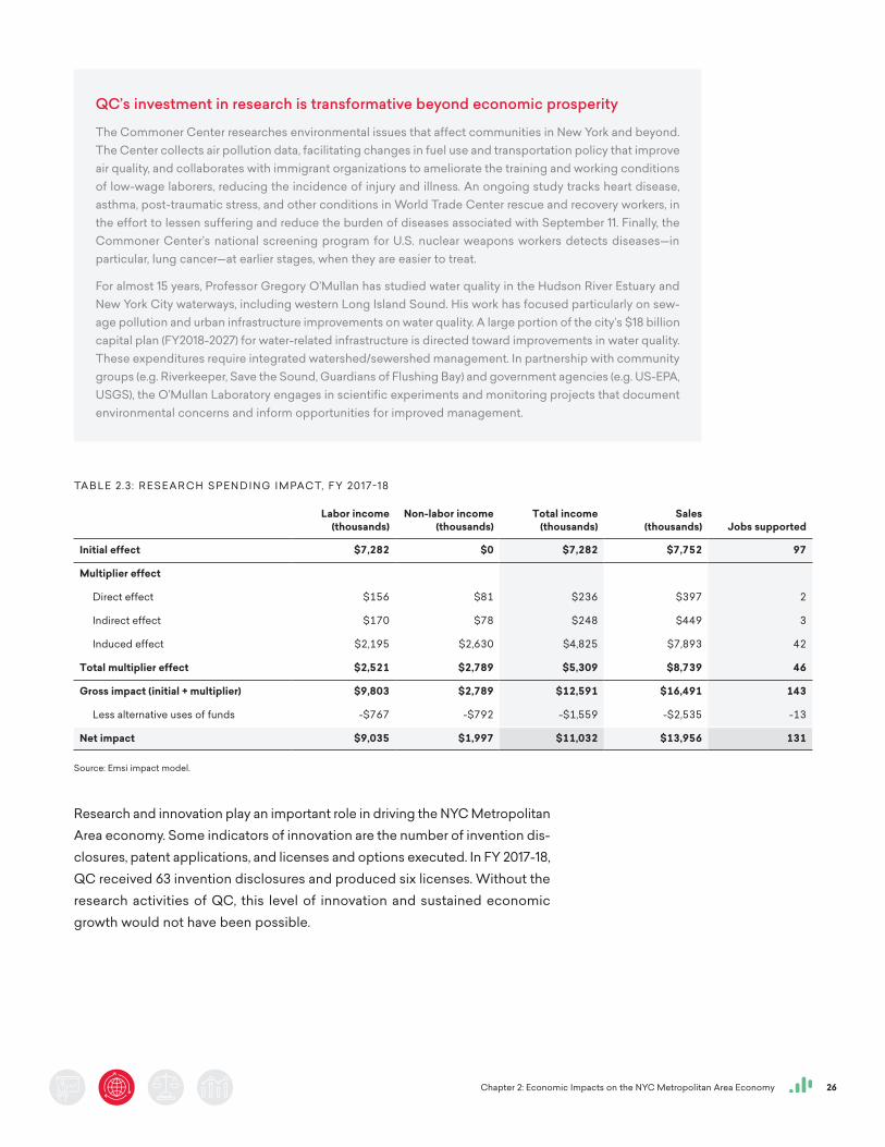
Initial, direct, indirect, and induced effects of QC’s research expenses appear in Table 2.3. As with the operations spending impact, the initial effect consists of the 97 research jobs and their associated salaries, wages, and benefits. The college’s research expenses have a total gross impact of $9.8 million in labor income and $2.8 million in non-labor income. This sums together to $12.6 mil-lion in added income, equivalent to 143 jobs. Taking into account the impact of the alternative uses of funds, net research expenditure impacts of QC are $9 million in labor income and $2 million in non-labor income. This sums together to $11 million in total added income and is equivalent to supporting 131 jobs.
16 The fields include environmental sciences, life sciences, math and computer sciences, physical sciences, psychol-ogy, social sciences, sciences not elsewhere classified, engineering, and all non-science and engineering fields.
F I G U R E 2.1 : R E S E A R C H E X P E N S E S BY F U N C T I O N ( M I L L I O N S)
2014
–15
2015
–16
2016
–17
2017
–18
Payroll
Pass-throughs
Equipment
Other
Source: Data provided by QC.
$25
$15
$10
$5
$0
$20
100+100+83+8656+56+47+4954+55+46+4842+41+35+38
Chapter 2: Economic Impacts on the NYC Metropolitan Area Economy 26
Research and innovation play an important role in driving the NYC Metropolitan Area economy. Some indicators of innovation are the number of invention dis-closures, patent applications, and licenses and options executed. In FY 2017-18, QC received 63 invention disclosures and produced six licenses. Without the research activities of QC, this level of innovation and sustained economic growth would not have been possible.
TA B L E 2.3 : R E S E A R C H S P E N D I N G I M PAC T, F Y 2017-18
Labor income
(thousands)Non-labor income
(thousands)Total income
(thousands)Sales
(thousands) Jobs supported
Initial effect $7,282 $0 $7,282 $7,752 97
Multiplier effect
Direct effect $156 $81 $236 $397 2
Indirect effect $170 $78 $248 $449 3
Induced effect $2,195 $2,630 $4,825 $7,893 42
Total multiplier effect $2,521 $2,789 $5,309 $8,739 46
Gross impact (initial + multiplier) $9,803 $2,789 $12,591 $16,491 143
Less alternative uses of funds -$767 -$792 -$1,559 -$2,535 -13
Net impact $9,035 $1,997 $11,032 $13,956 131
Source: Emsi impact model.
QC’s investment in research is transformative beyond economic prosperity
The Commoner Center researches environmental issues that affect communities in New York and beyond. The Center collects air pollution data, facilitating changes in fuel use and transportation policy that improve air quality, and collaborates with immigrant organizations to ameliorate the training and working conditions of low-wage laborers, reducing the incidence of injury and illness. An ongoing study tracks heart disease, asthma, post-traumatic stress, and other conditions in World Trade Center rescue and recovery workers, in the effort to lessen suffering and reduce the burden of diseases associated with September 11. Finally, the Commoner Center’s national screening program for U.S. nuclear weapons workers detects diseases—in particular, lung cancer—at earlier stages, when they are easier to treat.
For almost 15 years, Professor Gregory O’Mullan has studied water quality in the Hudson River Estuary and New York City waterways, including western Long Island Sound. His work has focused particularly on sew-age pollution and urban infrastructure improvements on water quality. A large portion of the city’s $18 billion capital plan (FY2018-2027) for water-related infrastructure is directed toward improvements in water quality. These expenditures require integrated watershed/sewershed management. In partnership with community groups (e.g. Riverkeeper, Save the Sound, Guardians of Flushing Bay) and government agencies (e.g. US-EPA, USGS), the O’Mullan Laboratory engages in scientific experiments and monitoring projects that document environmental concerns and inform opportunities for improved management.
Chapter 2: Economic Impacts on the NYC Metropolitan Area Economy 27
QC’s research activities create an economic impact beyond spending. There are impacts created through the entrepreneurial and innovative activities stemming from QC’s research. QC is leading innovation and research activities advancing sciences in music therapy, entomology, agroecology, among other cutting-edge research. However, the full magnitude of their value is difficult to quantify. Some of this value may be captured in the entrepreneurial and alumni impacts, presented later in this chapter. The broader spillover effects, however, remain as additional value created beyond the scope of this analysis.
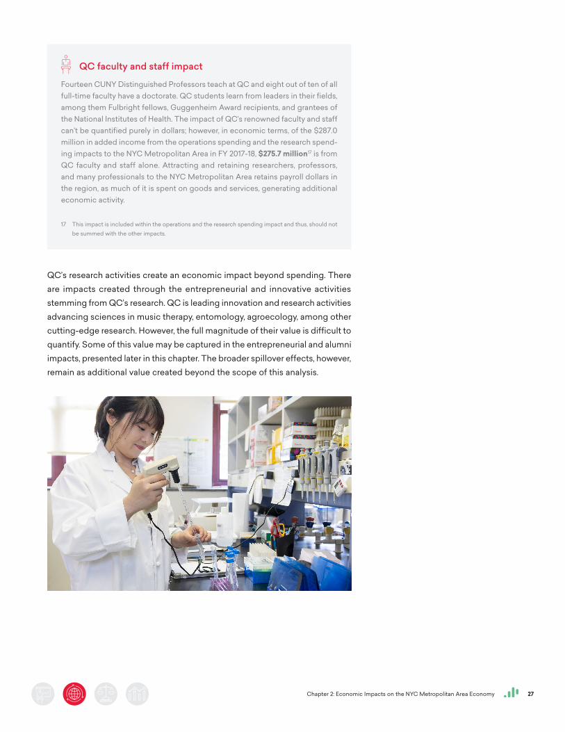
QC faculty and staff impact
Fourteen CUNY Distinguished Professors teach at QC and eight out of ten of all full-time faculty have a doctorate. QC students learn from leaders in their fields, among them Fulbright fellows, Guggenheim Award recipients, and grantees of the National Institutes of Health. The impact of QC’s renowned faculty and staff can’t be quantified purely in dollars; however, in economic terms, of the $287.0 million in added income from the operations spending and the research spend-ing impacts to the NYC Metropolitan Area in FY 2017-18, $275.7 million17 is from QC faculty and staff alone. Attracting and retaining researchers, professors, and many professionals to the NYC Metropolitan Area retains payroll dollars in the region, as much of it is spent on goods and services, generating additional economic activity.
17 This impact is included within the operations and the research spending impact and thus, should not be summed with the other impacts.
Chapter 2: Economic Impacts on the NYC Metropolitan Area Economy 28
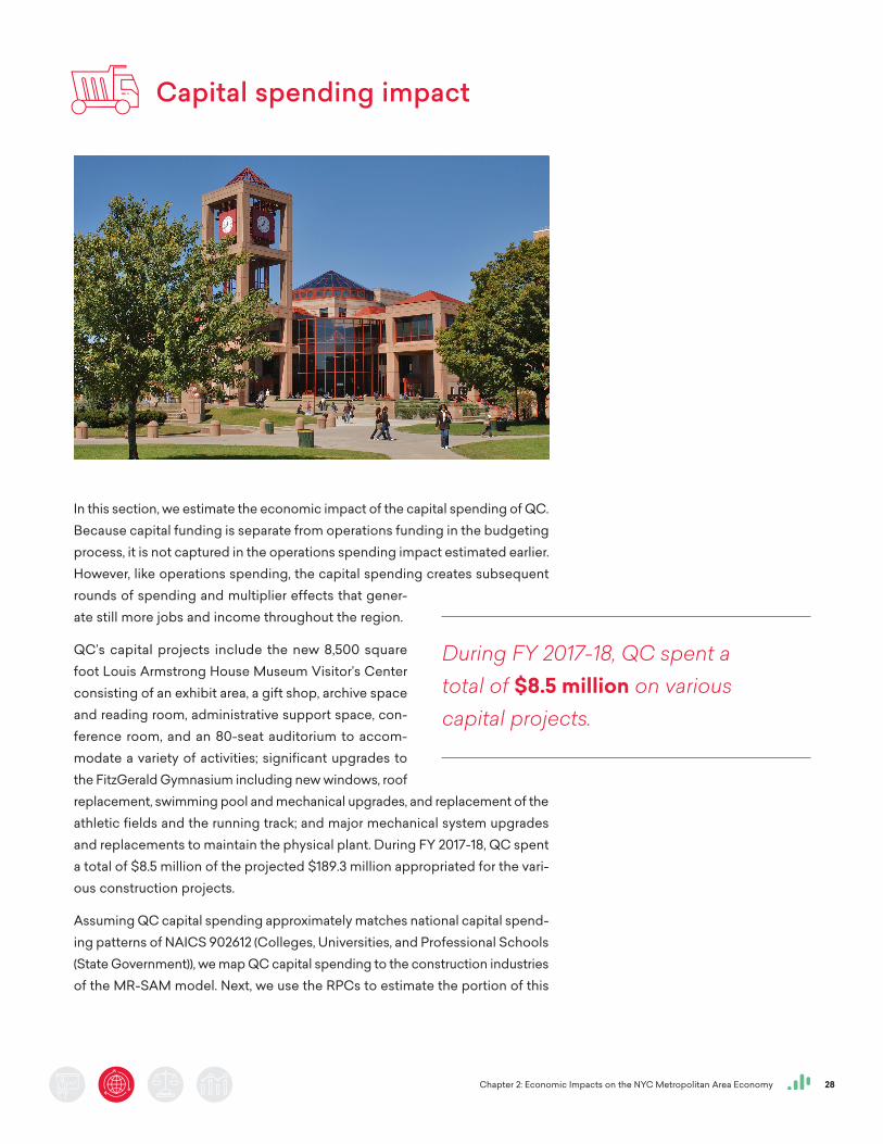
Capital spending impact
In this section, we estimate the economic impact of the capital spending of QC. Because capital funding is separate from operations funding in the budgeting process, it is not captured in the operations spending impact estimated earlier. However, like operations spending, the capital spending creates subsequent rounds of spending and multiplier effects that gener-ate still more jobs and income throughout the region.
QC’s capital projects include the new 8,500 square foot Louis Armstrong House Museum Visitor’s Center consisting of an exhibit area, a gift shop, archive space and reading room, administrative support space, con-ference room, and an 80-seat auditorium to accom-modate a variety of activities; significant upgrades to the FitzGerald Gymnasium including new windows, roof replacement, swimming pool and mechanical upgrades, and replacement of the athletic fields and the running track; and major mechanical system upgrades and replacements to maintain the physical plant. During FY 2017-18, QC spent a total of $8.5 million of the projected $189.3 million appropriated for the vari-ous construction projects.
Assuming QC capital spending approximately matches national capital spend-ing patterns of NAICS 902612 (Colleges, Universities, and Professional Schools (State Government)), we map QC capital spending to the construction industries of the MR-SAM model. Next, we use the RPCs to estimate the portion of this
During FY 2017-18, QC spent a total of $8.5 million on various capital projects.
Chapter 2: Economic Impacts on the NYC Metropolitan Area Economy 29
spending that occurs in-region. Finally, the in-region spending is run through the multiplier matrix to estimate the direct, indirect, and induced effects. Because construction is so labor intensive, the non-labor income impact is relatively small.
To account for the opportunity cost of any in-region construction money, we estimate the impacts of a similar alternative uses of funds as found in the operations and research spending impacts. This is done by simulating a scenario where in-region monies spent on construction are instead spent on consumer goods. These impacts are then subtracted from the gross capital spending impacts. Again, since construction is so labor intensive, most of the added income stems from labor income as opposed to non-labor income. As a result, the non-labor impacts associated with spending in the non-construction sectors are larger than in the construction sectors, so the net non-labor impact of capital spending is negative. This means that had the construction money instead been spent on consumer goods, more non-labor income would have been created at the expense of less labor income. The total net impact is still positive and substantial.
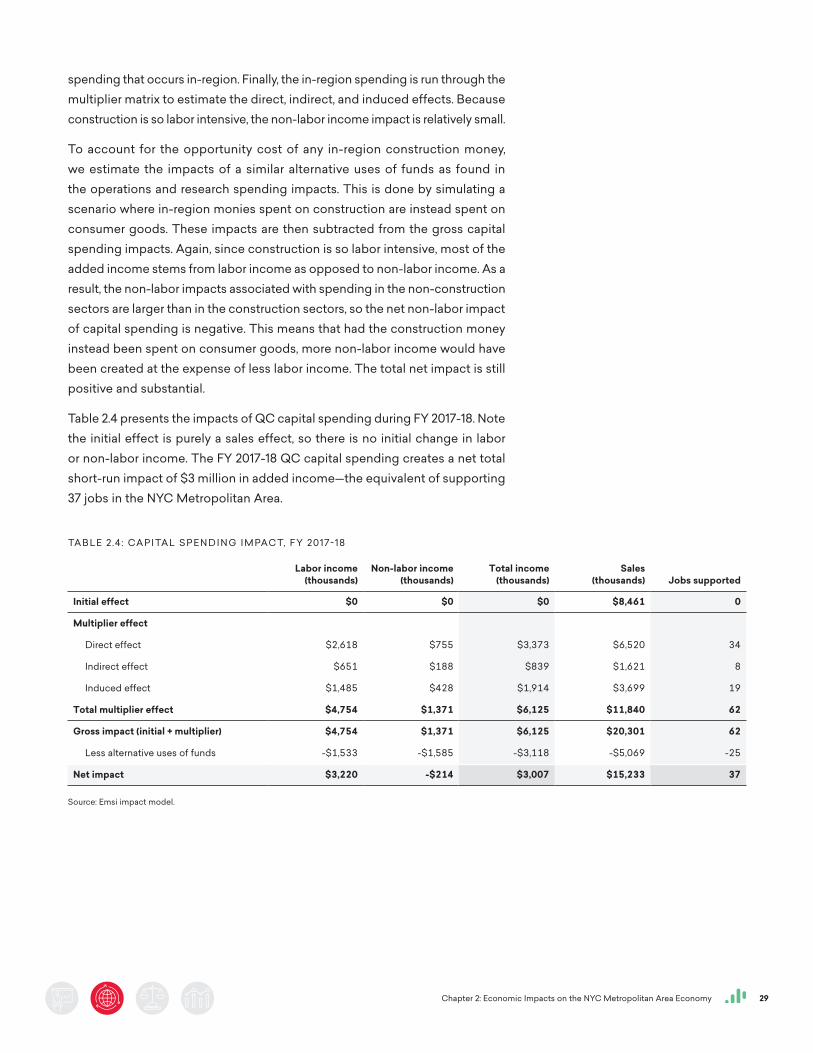
Table 2.4 presents the impacts of QC capital spending during FY 2017-18. Note the initial effect is purely a sales effect, so there is no initial change in labor or non-labor income. The FY 2017-18 QC capital spending creates a net total short-run impact of $3 million in added income—the equivalent of supporting 37 jobs in the NYC Metropolitan Area.
TA B L E 2.4: CA P I TA L S P E N D I N G I M PAC T, F Y 2017-18
Labor income
(thousands)Non-labor income
(thousands)Total income
(thousands)Sales
(thousands) Jobs supported
Initial effect $0 $0 $0 $8,461 0
Multiplier effect
Direct effect $2,618 $755 $3,373 $6,520 34
Indirect effect $651 $188 $839 $1,621 8
Induced effect $1,485 $428 $1,914 $3,699 19
Total multiplier effect $4,754 $1,371 $6,125 $11,840 62
Gross impact (initial + multiplier) $4,754 $1,371 $6,125 $20,301 62
Less alternative uses of funds -$1,533 -$1,585 -$3,118 -$5,069 -25
Net impact $3,220 -$214 $3,007 $15,233 37
Source: Emsi impact model.
Chapter 2: Economic Impacts on the NYC Metropolitan Area Economy 30
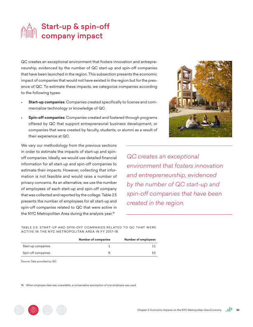
Start-up & spin-off company impact
QC creates an exceptional environment that fosters innovation and entrepre-neurship, evidenced by the number of QC start-up and spin-off companies that have been launched in the region. This subsection presents the economic impact of companies that would not have existed in the region but for the pres-ence of QC. To estimate these impacts, we categorize companies according to the following types:
• Start-up companies: Companies created specifically to license and com-mercialize technology or knowledge of QC.
• Spin-off companies: Companies created and fostered through programs offered by QC that support entrepreneurial business development, or companies that were created by faculty, students, or alumni as a result of their experience at QC.
We vary our methodology from the previous sections in order to estimate the impacts of start-up and spin-off companies. Ideally, we would use detailed financial information for all start-up and spin-off companies to estimate their impacts. However, collecting that infor-mation is not feasible and would raise a number of privacy concerns. As an alternative, we use the number of employees of each start-up and spin-off company that was collected and reported by the college. Table 2.5 presents the number of employees for all start-up and spin-off companies related to QC that were active in the NYC Metropolitan Area during the analysis year.18
18 When employee data was unavailable, a conservative assumption of one employee was used.
QC creates an exceptional environment that fosters innovation and entrepreneurship, evidenced by the number of QC start-up and spin-off companies that have been created in the region.
TA B L E 2.5 : S TA RT- U P A N D S P I N- O F F C O M PA N I E S R E L AT E D TO Q C T H AT W E R E AC T I V E I N T H E N YC M E T R O P O L I TA N A R E A I N F Y 2017-18
Number of companies Number of employees
Start-up companies 1 11
Spin-off companies 8 53
Source: Data provided by QC.
Chapter 2: Economic Impacts on the NYC Metropolitan Area Economy 31
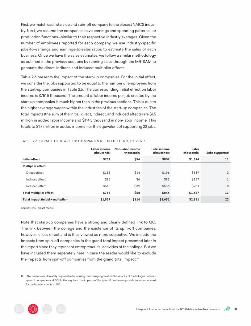
First, we match each start-up and spin-off company to the closest NAICS indus-try. Next, we assume the companies have earnings and spending patterns—or production functions—similar to their respective industry averages. Given the number of employees reported for each company, we use industry-specific jobs-to-earnings and earnings-to-sales ratios to estimate the sales of each business. Once we have the sales estimates, we follow a similar methodology as outlined in the previous sections by running sales through the MR-SAM to generate the direct, indirect, and induced multiplier effects.
Table 2.6 presents the impact of the start-up companies. For the initial effect, we consider the jobs supported to be equal to the number of employees from the start-up companies in Table 2.5. The corresponding initial effect on labor income is $751.5 thousand. The amount of labor income per job created by the start-up companies is much higher than in the previous sections. This is due to the higher average wages within the industries of the start-up companies. The total impacts (the sum of the initial, direct, indirect, and induced effects) are $1.5 million in added labor income and $114.5 thousand in non-labor income. This totals to $1.7 million in added income—or the equivalent of supporting 22 jobs.
Note that start-up companies have a strong and clearly defined link to QC. The link between the college and the existence of its spin-off companies, however, is less direct and is thus viewed as more subjective. We include the impacts from spin-off companies in the grand total impact presented later in the report since they represent entrepreneurial activities of the college. But we have included them separately here in case the reader would like to exclude the impacts from spin-off companies from the grand total impact.19
19 The readers are ultimately responsible for making their own judgment on the veracity of the linkages between spin-off companies and QC. At the very least, the impacts of the spin-off businesses provide important context for the broader effects of QC.
TA B L E 2.6: I M PAC T O F S TA RT- U P C O M PA N I E S R E L AT E D TO Q C, F Y 2017-18
Labor income
(thousands)Non-labor income
(thousands)Total income
(thousands)Sales
(thousands) Jobs supported
Initial effect $751 $56 $807 $1,394 11
Multiplier effect
Direct effect $183 $14 $196 $339 3
Indirect effect $85 $6 $91 $157 1
Induced effect $518 $39 $556 $961 8
Total multiplier effect $785 $58 $844 $1,457 11
Total impact (initial + multiplier) $1,537 $114 $1,651 $2,851 22
Source: Emsi impact model.
Chapter 2: Economic Impacts on the NYC Metropolitan Area Economy 32
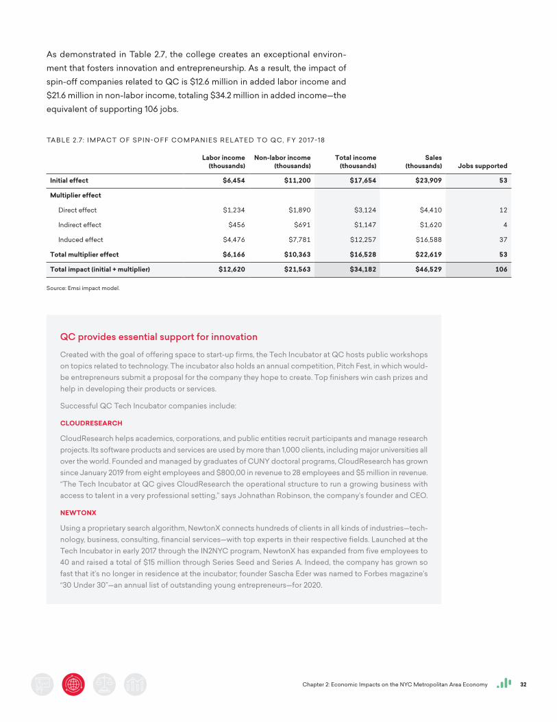
As demonstrated in Table 2.7, the college creates an exceptional environ-ment that fosters innovation and entrepreneurship. As a result, the impact of spin-off companies related to QC is $12.6 million in added labor income and $21.6 million in non-labor income, totaling $34.2 million in added income—the equivalent of supporting 106 jobs.
TA B L E 2.7 : I M PAC T O F S P I N- O F F C O M PA N I E S R E L AT E D TO Q C, F Y 2017-18
Labor income
(thousands)Non-labor income
(thousands)Total income
(thousands)Sales
(thousands) Jobs supported
Initial effect $6,454 $11,200 $17,654 $23,909 53
Multiplier effect
Direct effect $1,234 $1,890 $3,124 $4,410 12
Indirect effect $456 $691 $1,147 $1,620 4
Induced effect $4,476 $7,781 $12,257 $16,588 37
Total multiplier effect $6,166 $10,363 $16,528 $22,619 53
Total impact (initial + multiplier) $12,620 $21,563 $34,182 $46,529 106
Source: Emsi impact model.
QC provides essential support for innovation
Created with the goal of offering space to start-up firms, the Tech Incubator at QC hosts public workshops on topics related to technology. The incubator also holds an annual competition, Pitch Fest, in which would-be entrepreneurs submit a proposal for the company they hope to create. Top finishers win cash prizes and help in developing their products or services.
Successful QC Tech Incubator companies include:
CLOUDRESEARCH
CloudResearch helps academics, corporations, and public entities recruit participants and manage research projects. Its software products and services are used by more than 1,000 clients, including major universities all over the world. Founded and managed by graduates of CUNY doctoral programs, CloudResearch has grown since January 2019 from eight employees and $800,00 in revenue to 28 employees and $5 million in revenue. “The Tech Incubator at QC gives CloudResearch the operational structure to run a growing business with access to talent in a very professional setting,” says Johnathan Robinson, the company’s founder and CEO.
NEWTONX
Using a proprietary search algorithm, NewtonX connects hundreds of clients in all kinds of industries—tech-nology, business, consulting, financial services—with top experts in their respective fields. Launched at the Tech Incubator in early 2017 through the IN2NYC program, NewtonX has expanded from five employees to 40 and raised a total of $15 million through Series Seed and Series A. Indeed, the company has grown so fast that it’s no longer in residence at the incubator; founder Sascha Eder was named to Forbes magazine’s “30 Under 30”—an annual list of outstanding young entrepreneurs—for 2020.
Chapter 2: Economic Impacts on the NYC Metropolitan Area Economy 33
Visitor spending impact
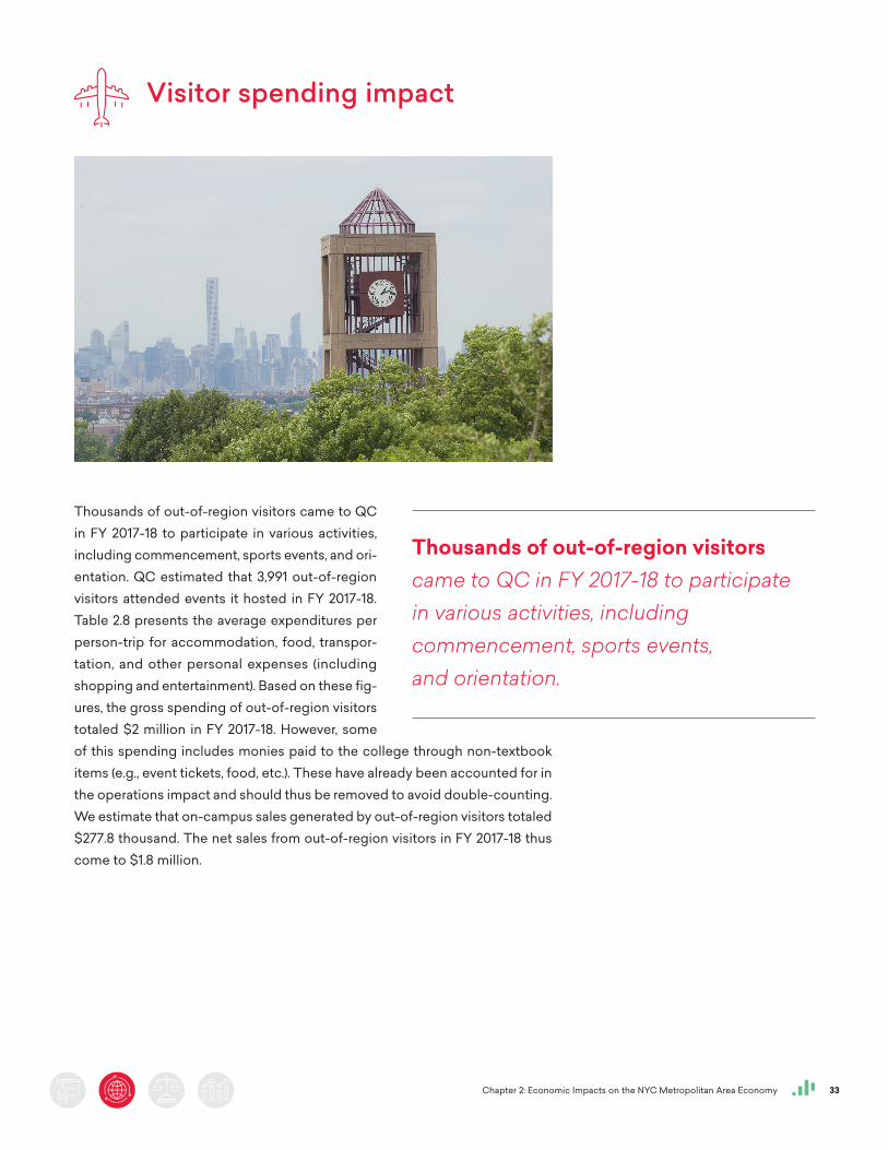
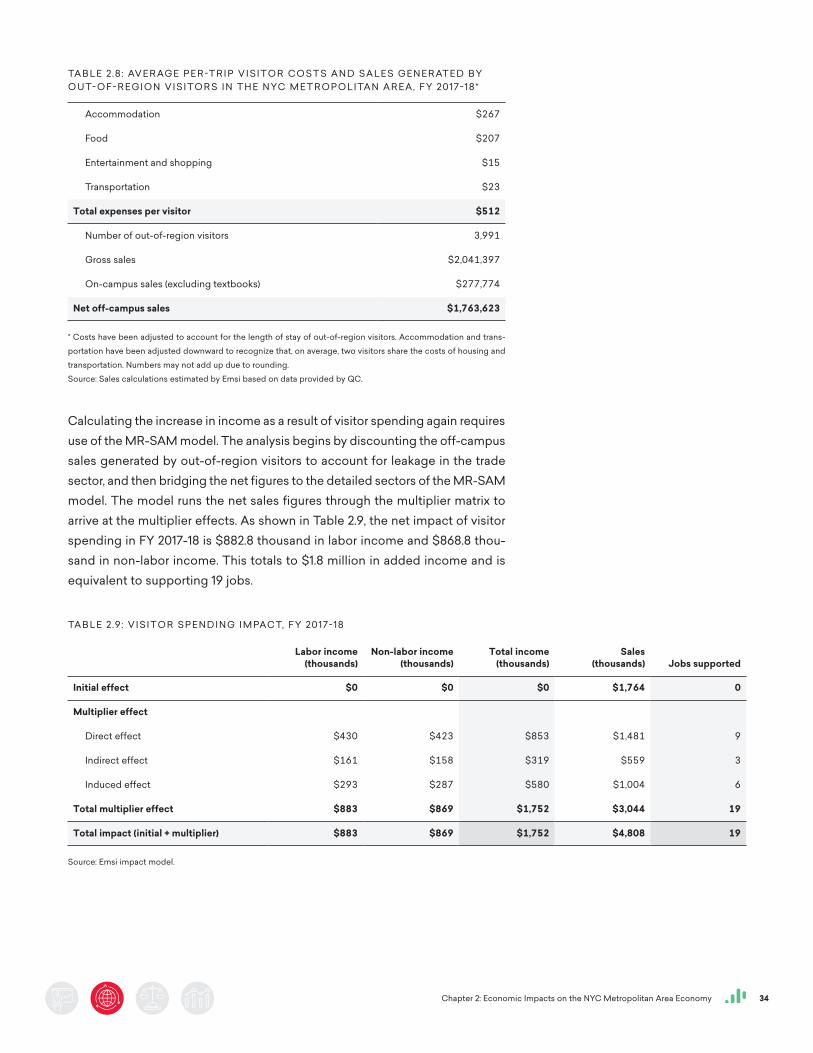
Thousands of out-of-region visitors came to QC in FY 2017-18 to participate in various activities, including commencement, sports events, and ori-entation. QC estimated that 3,991 out-of-region visitors attended events it hosted in FY 2017-18. Table 2.8 presents the average expenditures per person-trip for accommodation, food, transpor-tation, and other personal expenses (including shopping and entertainment). Based on these fig-ures, the gross spending of out-of-region visitors totaled $2 million in FY 2017-18. However, some of this spending includes monies paid to the college through non-textbook items (e.g., event tickets, food, etc.). These have already been accounted for in the operations impact and should thus be removed to avoid double-counting. We estimate that on-campus sales generated by out-of-region visitors totaled $277.8 thousand. The net sales from out-of-region visitors in FY 2017-18 thus come to $1.8 million.
Thousands of out-of-region visitors came to QC in FY 2017-18 to participate in various activities, including commencement, sports events, and orientation.
Chapter 2: Economic Impacts on the NYC Metropolitan Area Economy 34
Calculating the increase in income as a result of visitor spending again requires use of the MR-SAM model. The analysis begins by discounting the off-campus sales generated by out-of-region visitors to account for leakage in the trade sector, and then bridging the net figures to the detailed sectors of the MR-SAM model. The model runs the net sales figures through the multiplier matrix to arrive at the multiplier effects. As shown in Table 2.9, the net impact of visitor spending in FY 2017-18 is $882.8 thousand in labor income and $868.8 thou-sand in non-labor income. This totals to $1.8 million in added income and is equivalent to supporting 19 jobs.
TA B L E 2.9: V I S I TO R S P E N D I N G I M PAC T, F Y 2017-18
Labor income
(thousands)Non-labor income
(thousands)Total income
(thousands)Sales
(thousands) Jobs supported
Initial effect $0 $0 $0 $1,764 0
Multiplier effect
Direct effect $430 $423 $853 $1,481 9
Indirect effect $161 $158 $319 $559 3
Induced effect $293 $287 $580 $1,004 6
Total multiplier effect $883 $869 $1,752 $3,044 19
Total impact (initial + multiplier) $883 $869 $1,752 $4,808 19
Source: Emsi impact model.
TA B L E 2.8: AV E R AG E P E R-T R I P V I S I TO R C O S T S A N D SA L E S G E N E R AT E D BY O U T- O F- R E G I O N V I S I TO R S I N T H E N YC M E T R O P O L I TA N A R E A, F Y 2017-18*
Accommodation $267
Food $207
Entertainment and shopping $15
Transportation $23
Total expenses per visitor $512
Number of out-of-region visitors 3,991
Gross sales $2,041,397
On-campus sales (excluding textbooks) $277,774
Net off-campus sales $1,763,623
* Costs have been adjusted to account for the length of stay of out-of-region visitors. Accommodation and trans-
portation have been adjusted downward to recognize that, on average, two visitors share the costs of housing and
transportation. Numbers may not add up due to rounding.
Source: Sales calculations estimated by Emsi based on data provided by QC.
Chapter 2: Economic Impacts on the NYC Metropolitan Area Economy 35
Student spending impact
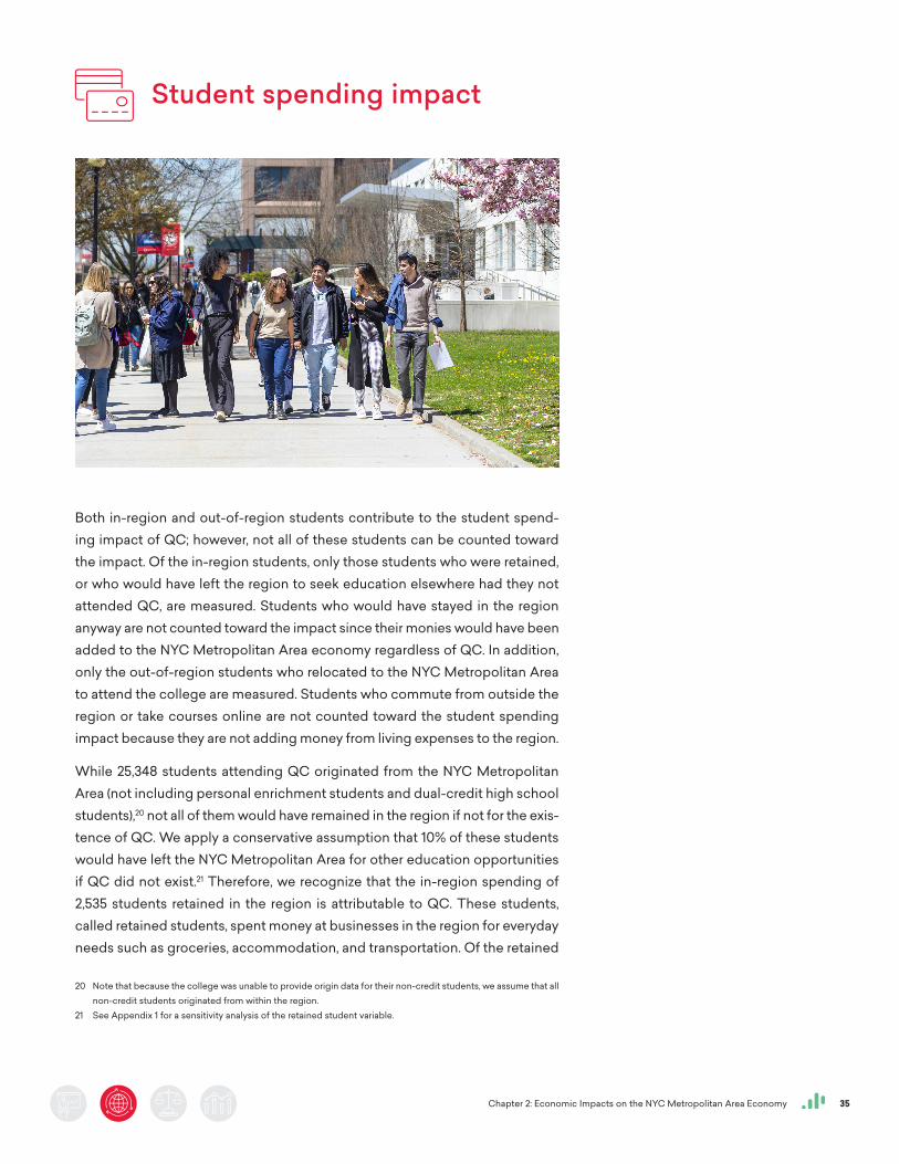
Both in-region and out-of-region students contribute to the student spend-ing impact of QC; however, not all of these students can be counted toward the impact. Of the in-region students, only those students who were retained, or who would have left the region to seek education elsewhere had they not attended QC, are measured. Students who would have stayed in the region anyway are not counted toward the impact since their monies would have been added to the NYC Metropolitan Area economy regardless of QC. In addition, only the out-of-region students who relocated to the NYC Metropolitan Area to attend the college are measured. Students who commute from outside the region or take courses online are not counted toward the student spending impact because they are not adding money from living expenses to the region.
While 25,348 students attending QC originated from the NYC Metropolitan Area (not including personal enrichment students and dual-credit high school students),20 not all of them would have remained in the region if not for the exis-tence of QC. We apply a conservative assumption that 10% of these students would have left the NYC Metropolitan Area for other education opportunities if QC did not exist.21 Therefore, we recognize that the in-region spending of 2,535 students retained in the region is attributable to QC. These students, called retained students, spent money at businesses in the region for everyday needs such as groceries, accommodation, and transportation. Of the retained
20 Note that because the college was unable to provide origin data for their non-credit students, we assume that all non-credit students originated from within the region.
21 See Appendix 1 for a sensitivity analysis of the retained student variable.
Chapter 2: Economic Impacts on the NYC Metropolitan Area Economy 36
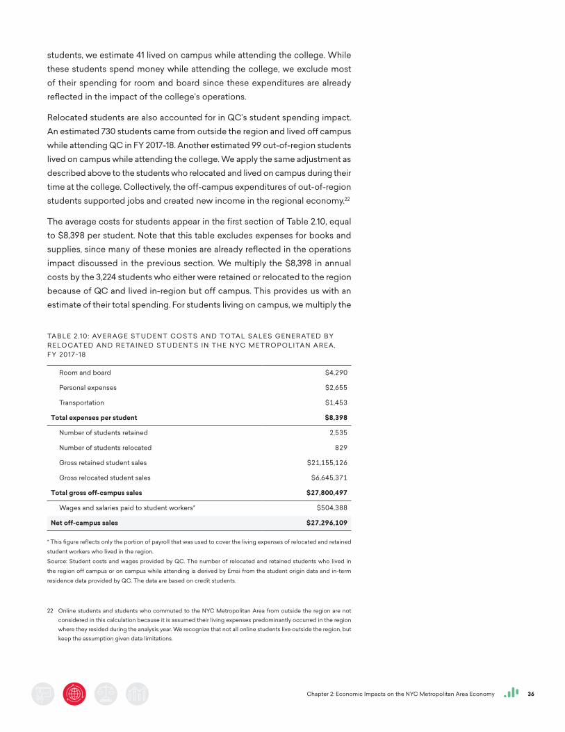
students, we estimate 41 lived on campus while attending the college. While these students spend money while attending the college, we exclude most of their spending for room and board since these expenditures are already reflected in the impact of the college’s operations.
Relocated students are also accounted for in QC’s student spending impact. An estimated 730 students came from outside the region and lived off campus while attending QC in FY 2017-18. Another estimated 99 out-of-region students lived on campus while attending the college. We apply the same adjustment as described above to the students who relocated and lived on campus during their time at the college. Collectively, the off-campus expenditures of out-of-region students supported jobs and created new income in the regional economy.22
The average costs for students appear in the first section of Table 2.10, equal to $8,398 per student. Note that this table excludes expenses for books and supplies, since many of these monies are already reflected in the operations impact discussed in the previous section. We multiply the $8,398 in annual costs by the 3,224 students who either were retained or relocated to the region because of QC and lived in-region but off campus. This provides us with an estimate of their total spending. For students living on campus, we multiply the
22 Online students and students who commuted to the NYC Metropolitan Area from outside the region are not considered in this calculation because it is assumed their living expenses predominantly occurred in the region where they resided during the analysis year. We recognize that not all online students live outside the region, but keep the assumption given data limitations.
TA B L E 2.10: AV E R AG E S T U D E N T C O S T S A N D TOTA L SA L E S G E N E R AT E D BY R E LO CAT E D A N D R E TA I N E D S T U D E N T S I N T H E N YC M E T R O P O L I TA N A R E A, F Y 2017-18
Room and board $4,290
Personal expenses $2,655
Transportation $1,453
Total expenses per student $8,398
Number of students retained 2,535
Number of students relocated 829
Gross retained student sales $21,155,126
Gross relocated student sales $6,645,371
Total gross off-campus sales $27,800,497
Wages and salaries paid to student workers* $504,388
Net off-campus sales $27,296,109
* This figure reflects only the portion of payroll that was used to cover the living expenses of relocated and retained
student workers who lived in the region.
Source: Student costs and wages provided by QC. The number of relocated and retained students who lived in
the region off campus or on campus while attending is derived by Emsi from the student origin data and in-term
residence data provided by QC. The data are based on credit students.
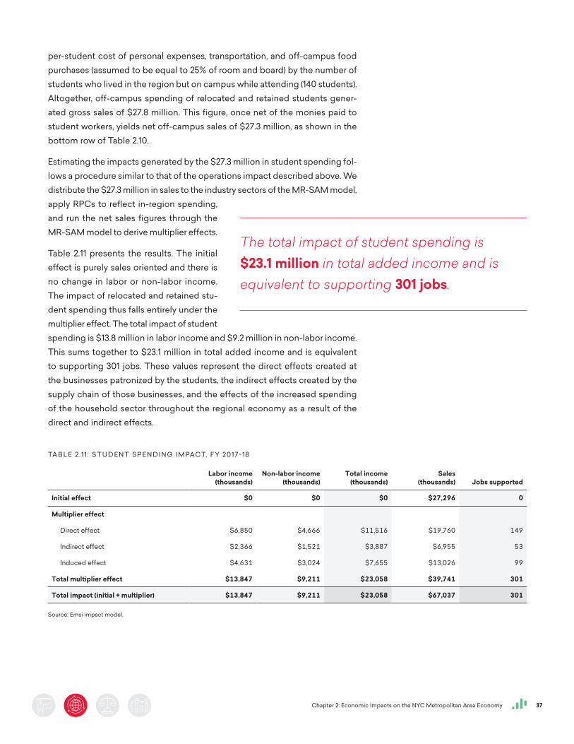
Chapter 2: Economic Impacts on the NYC Metropolitan Area Economy 37
per-student cost of personal expenses, transportation, and off-campus food purchases (assumed to be equal to 25% of room and board) by the number of students who lived in the region but on campus while attending (140 students). Altogether, off-campus spending of relocated and retained students gener-ated gross sales of $27.8 million. This figure, once net of the monies paid to student workers, yields net off-campus sales of $27.3 million, as shown in the bottom row of Table 2.10.
Estimating the impacts generated by the $27.3 million in student spending fol-lows a procedure similar to that of the operations impact described above. We distribute the $27.3 million in sales to the industry sectors of the MR-SAM model, apply RPCs to reflect in-region spending, and run the net sales figures through the MR-SAM model to derive multiplier effects.
Table 2.11 presents the results. The initial effect is purely sales oriented and there is no change in labor or non-labor income. The impact of relocated and retained stu-dent spending thus falls entirely under the multiplier effect. The total impact of student spending is $13.8 million in labor income and $9.2 million in non-labor income. This sums together to $23.1 million in total added income and is equivalent to supporting 301 jobs. These values represent the direct effects created at the businesses patronized by the students, the indirect effects created by the supply chain of those businesses, and the effects of the increased spending of the household sector throughout the regional economy as a result of the direct and indirect effects.
TA B L E 2.11 : S T U D E N T S P E N D I N G I M PAC T, F Y 2017-18
Labor income
(thousands)Non-labor income
(thousands)Total income
(thousands)Sales
(thousands) Jobs supported
Initial effect $0 $0 $0 $27,296 0
Multiplier effect
Direct effect $6,850 $4,666 $11,516 $19,760 149
Indirect effect $2,366 $1,521 $3,887 $6,955 53
Induced effect $4,631 $3,024 $7,655 $13,026 99
Total multiplier effect $13,847 $9,211 $23,058 $39,741 301
Total impact (initial + multiplier) $13,847 $9,211 $23,058 $67,037 301
Source: Emsi impact model.
The total impact of student spending is $23.1 million in total added income and is equivalent to supporting 301 jobs.
Chapter 2: Economic Impacts on the NYC Metropolitan Area Economy 38
Alumni impact
In this section, we estimate the economic impacts stemming from the added labor income of alumni in combination with their employers’ added non-labor income. This impact is based on the number of students who have attended QC throughout its history. We then use this total number to consider the impact of those students in the single FY 2017-18. Former students who earned a degree as well as those who may not have finished their degree or did not take courses for credit are considered alumni.
While QC creates an economic impact through its operations, research, capital, entrepreneurial, visitor, and student spending, the greatest economic impact of QC stems from the added human capital—the knowledge, creativity, imagination, and entrepreneurship—found in its alumni. This increase in creativity translated into productivity is exemplified by QC’s alumni in the arts, as published by a federal government study of the arts.23 While attending QC, students gain expe-rience, education, and the knowledge, skills, and abilities that increase their productivity and allow them to com-mand a higher wage once they enter the workforce. But the reward of increased productivity does not stop there. Talented professionals make capital more productive, too (e.g., buildings, production facilities, equipment). The employers of QC alumni enjoy the fruits of this increased productivity in the form of additional non-labor income (i.e., higher profits).
The methodology here differs from the previous impacts in one fundamental way. Whereas the previous spending impacts depend on an annually renewed injection of new sales into the regional economy, the alumni impact is the result of years of past instruction and the associated accumulation of human capital. The initial effect of alumni compromises two main components. The first and largest of these is the added labor income of QC’s former students. The second component of the initial effect comprises the added non-labor income of the businesses that employ former students of QC.
We begin by estimating the portion of alumni who are employed in the work-force. To estimate the historical employment patterns of alumni in the region, we use the following sets of data or assumptions: 1) settling-in factors to determine
23 QC alumni in the arts contribute to the overall economic impact of the arts industries, as cited by https://www.newyorkupstate.com/news/2018/04/study_ny_states_arts_cultural_industries_have_114_billion_impact.html
The greatest economic impact of QC stems from the added human capital—the knowledge, creativity, imagination, and entrepreneurship—found in its alumni.
Chapter 2: Economic Impacts on the NYC Metropolitan Area Economy 39
how long it takes the average student to settle into a career;24 2) death, retire-ment, and unemployment rates from the National Center for Health Statistics, the Social Security Administration, and the Bureau of Labor Statistics; and 3) state migration data from the Census Bureau. The result is the estimated portion of alumni from each previous year who were still actively employed in the region as of FY 2017-18.
The next step is to quantify the skills and human capital that alumni acquired from the college. We use the students’ production of CHEs as a proxy for accu-mulated human capital. The average number of CHEs completed per student in FY 2017-18 was 15.2. To estimate the number of CHEs present in the workforce during the analysis year, we use the college’s historical student headcount over the past 30 years, from FY 1988-89 to FY 2017-18.25 We multiply the 15.2 average CHEs per student by the headcounts that we estimate are still actively employed from each of the previous years.26 Students who enroll at the college for more than one year are counted at least twice in the historical enrollment data. However, CHEs remain distinct regardless of when and by whom they were earned, so there is no duplication in the CHE counts. We estimate there are approximately 5.4 million CHEs from alumni active in the workforce.
Next, we estimate the value of the CHEs, or the skills and human capital acquired by QC alumni. This is done using the incremental added labor income stem-ming from the students’ higher wages. The incremental added labor income is the difference between the wage earned by QC alumni and the alternative wage they would have earned had they not attended QC. Using the regional incremental earnings, credits required, and distribution of credits at each level of study, we estimate the average value per CHE to equal $237. This value rep-resents the regional average incremental increase in wages that alumni of QC received during the analysis year for every CHE they completed.
Because workforce experience leads to increased productivity and higher wages, the value per CHE varies depending on the students’ workforce expe-rience, with the highest value applied to the CHEs of students who had been employed the longest by FY 2017-18, and the lowest value per CHE applied to students who were just entering the workforce. More information on the theory and calculations behind the value per CHE appears in Appendix 6. In determining the amount of added labor income attributable to alumni, we multiply the CHEs of former students in each year of the historical time horizon
24 Settling-in factors are used to delay the onset of the benefits to students in order to allow time for them to find employment and settle into their careers. In the absence of hard data, we assume a range between one and three years for students who graduate with a certificate or a degree, and between one and five years for returning students.
25 We apply a 30-year time horizon because the data on students who attended QC prior to FY 1988-89 is less reliable, and because most of the students served more than 30 years ago had left the regional workforce by FY 2017-18.
26 This assumes the average credit load and level of study from past years is equal to the credit load and level of study of students today.
Lilo Leeds ’48
Co-founded CMP Publications Inc. with her husband Gerry in 1971, special-izing in trade magazines that covered business and technology. Some 25 years later, the Manhasset-based com-pany recorded $480 million in annual revenue and had a payroll of more than 1,700 people. In 1999, after taking CMP public, the Leeds family sold it for $920 million, sharing $50 million with employees. Lilo, who had fled Germany with her family in 1933, devoted the rest of her career to philanthropy: She and her husband co-founded several organi-zations designed to help disadvantaged students succeed in school. She passed away in 2016.
Sara Miller McCune ’61
Founded SAGE Publications in 1965 to enable scholars to disseminate quality research in their own voices. Now known as SAGE Publishing and headquartered in Thousand Oaks, California, the company has additional offices in North America, Europe, Asia, and Australia, and employs over 1,500 around the world. SAGE’s products range from books and journals to online courses and technologies for learning and research. McCune is committed to funding grassroots projects that advance educational opportunities for underserved communities. She is also a passionate supporter of the arts, an active advocate for social issues, and a long-term sponsor of academic and university initiatives.
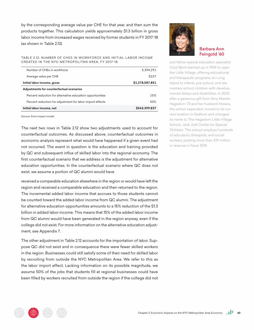
Chapter 2: Economic Impacts on the NYC Metropolitan Area Economy 40
by the corresponding average value per CHE for that year, and then sum the products together. This calculation yields approximately $1.3 billion in gross labor income from increased wages received by former students in FY 2017-18 (as shown in Table 2.12).
The next two rows in Table 2.12 show two adjustments used to account for counterfactual outcomes. As discussed above, counterfactual outcomes in economic analysis represent what would have happened if a given event had not occurred. The event in question is the education and training provided by QC and subsequent influx of skilled labor into the regional economy. The first counterfactual scenario that we address is the adjustment for alternative education opportunities. In the counterfactual scenario where QC does not exist, we assume a portion of QC alumni would have
received a comparable education elsewhere in the region or would have left the region and received a comparable education and then returned to the region. The incremental added labor income that accrues to those students cannot be counted toward the added labor income from QC alumni. The adjustment for alternative education opportunities amounts to a 15% reduction of the $1.3 billion in added labor income. This means that 15% of the added labor income from QC alumni would have been generated in the region anyway, even if the college did not exist. For more information on the alternative education adjust-ment, see Appendix 7.
The other adjustment in Table 2.12 accounts for the importation of labor. Sup-pose QC did not exist and in consequence there were fewer skilled workers in the region. Businesses could still satisfy some of their need for skilled labor by recruiting from outside the NYC Metropolitan Area. We refer to this as the labor import effect. Lacking information on its possible magnitude, we assume 50% of the jobs that students fill at regional businesses could have been filled by workers recruited from outside the region if the college did not
TA B L E 2.12 : N U M B E R O F C H E S I N WO R K F O R C E A N D I N I T I A L L A B O R I N C O M E C R E AT E D I N T H E N YC M E T R O P O L I TA N A R E A, F Y 2017-18
Number of CHEs in workforce 5,394,291
Average value per CHE $237
Initial labor income, gross $1,278,587,851
Adjustments for counterfactual scenarios
Percent reduction for alternative education opportunities 15%
Percent reduction for adjustment for labor import effects 50%
Initial labor income, net $543,399,837
Source: Emsi impact model.
Barbara Ann Feingold ’60
and fellow special education specialist Caryl Bank teamed up in 1969 to open the Little Village, offering educational and therapeutic programs on Long Island to infants, pre-school, and ele-mentary school children with develop-mental delays and disabilities. In 2002, after a generous gift from Amy Maiello Hagedorn ’73 and her husband Horace, the school expanded, moved to its cur-rent location in Seaford, and changed its name to The Hagedorn Little Village School, Jack Joel Center for Special Children. The school employs hundreds of educators, therapists, and social workers, posting more than $19 million in revenue in fiscal 2019.
Chapter 2: Economic Impacts on the NYC Metropolitan Area Economy 41
exist.27 Consequently, the gross labor income must be adjusted to account for the importation of this labor, since it would have happened regardless of the presence of the college. We conduct a sensitivity analysis for this assumption in Appendix 1. With the 50% adjustment, the net added labor income added to the economy comes to $543.4 million, as shown in Table 2.12.
The $543.4 million in added labor income appears under the initial effect in the labor income column of Table 2.13. To this we add an estimate for initial non-labor income. As discussed earlier in this section, businesses that employ former students of QC see higher profits as a result of the increased productiv-ity of their capital assets. To estimate this additional income, we allocate the initial increase in labor income ($543.4 million) to the six-digit NAICS industry sectors where students are most likely to be employed. This allocation entails a process that maps completers in the region to the detailed occupations for which those completers have been trained, and then maps the detailed occupations to the six-digit industry sectors in the MR-SAM model.28 Using a crosswalk created by National Center for Education Statistics (NCES) and the Bureau of Labor Statistics, we map the breakdown of the college’s completers to the approximately 700 detailed occupations in the Standard Occupational Classification (SOC) system. Finally, we apply a matrix of wages by industry and by occupation from the MR-SAM model to map the occupational distribution of the $543.4 million in initial labor income effects to the detailed industry sectors in the MR-SAM model.29
Once these allocations are complete, we apply the ratio of non-labor to labor income provided by the MR-SAM model for each sector to our estimate of initial labor income. This computation yields an estimated $171.9 million in added non-labor income attributable to the college’s alumni. Summing initial labor and non-labor income together provides the total initial effect of alumni productivity in the NYC Metropolitan Area economy, equal to approximately $715.3 million. To estimate multiplier effects, we convert the industry-specific income figures generated through the initial effect to sales using sales-to-income ratios from the MR-SAM model. We then run the values through the MR-SAM’s multiplier matrix.
Table 2.13 shows the multiplier effects of alumni. Multiplier effects occur as alumni generate an increased demand for consumer goods and services through the expenditure of their higher wages. Further, as the industries where alumni
27 A similar assumption is used by Walden (2014) in his analysis of the Cooperating Raleigh Colleges.28 Completer data comes from the Integrated Postsecondary Education Data System (IPEDS), which organizes
program completions according to the Classification of Instructional Programs (CIP) developed by the National Center for Education Statistics (NCES).
29 For example, if the MR-SAM model indicates that 20% of wages paid to workers in SOC 51-4121 (Welders) occur in NAICS 332313 (Plate Work Manufacturing), then we allocate 20% of the initial labor income effect under SOC 51-4121 to NAICS 332313.
Directly from employers
Our firm has had a long-standing rela-tionship with QC students, specifically with the Center for Career Engagement & Internships. Our interaction with the Center for Career Engagement & Internships team has been outstanding as they genuinely want their students to succeed beyond QC. QC continues to be an organization where we seek to attract talent as the students have a strong work ethic, come from diverse backgrounds, and have a sense of pride in their QC roots. It’s consistently a positive recruiting experience for full-time new hire and internship recruits.
— Jennifer Rambarran, PwC
QC’s mission to have “students graduate with the ability to think critically, address complex problems, explore various cultures, and use modern technologies and information resources” is the exact reason why GEICO recruits there. The student’s varied backgrounds and cultures stimulate diverse conversations and ideas that, along with their critical thinking skills and strong work ethic, meld well into GEICO’s culture.
— Jeanne Toscano, GEICO
Chapter 2: Economic Impacts on the NYC Metropolitan Area Economy 42
are employed increase their output, there is a corresponding increase in the demand for input from the industries in the employers’ supply chain. Together, the incomes generated by the expansions in business input purchases and household spending constitute the multiplier effect of the increased produc-tivity of the college’s alumni. The final results are $562.6 million in added labor income and $176.1 million in added non-labor income, for an overall total of $738.8 million in multiplier effects. The grand total of the alumni impact is $1.5 billion in total added income, the sum of all initial and multiplier labor and non-labor income effects. This is equivalent to supporting 12,843 jobs.
TA B L E 2.13 : A L U M N I I M PAC T, F Y 2017-18
Labor income
(thousands)Non-labor income
(thousands)Total income
(thousands)Sales
(thousands) Jobs supported
Initial effect $543,400 $171,853 $715,252 $1,287,577 6,217
Multiplier effect
Direct effect $98,958 $40,032 $138,990 $243,740 1,197
Indirect effect $39,671 $16,814 $56,485 $100,748 501
Induced effect $424,017 $119,273 $543,289 $906,464 4,929
Total multiplier effect $562,645 $176,119 $738,764 $1,250,952 6,627
Total impact (initial + multiplier) $1,106,045 $347,972 $1,454,016 $2,538,529 12,843
Source: Emsi impact model.
QC’s alumni create jobs
Max Kupferberg ’42, who passed away in 2017 at the age of 97, had an immeasurable impact on the Queens community as both a businessman and a philanthropist.
A member of QC’s first incoming class, Kupferberg studied physics at QC and went on to work on the top-secret Manhattan Project during World War II. In 1946, a year after the war ended, he opened Kepco, Inc. with his three brothers. They set up shop in Flushing, designing and manufacturing DC power supplies and associated electronic equipment. Their instrument products are found in automatic test equipment, avionics, aerospace,
experimental electronics, and high-energy physics applications, and many of their designs led to technological advancements in the industry. More than 70 years later, Kepco remains a family-operated business in Queens.
In 2006, Kupferberg and his wife, Selma, donated $10 million to support arts programs at QC. Named in their honor, the Kupferberg Center for the Arts encompasses Colden Auditorium, the Godwin-Ternbach Museum, the Queens College Art Center, and the Louis Armstrong House Museum and Archives. Each year, the center hosts concerts and exhibitions by world-class performers, outstanding regional and local artists, and QC students and faculty.

Chapter 2: Economic Impacts on the NYC Metropolitan Area Economy 43
Sara Radicati ’77 started her eponymous market research firm in 1993 to focus on mes-saging and collaboration. Today, the Radicati Group provides quantitative and qualitative research on email, security, instant messaging, social networking, information archiving, regulatory compliance, wireless technologies, web technologies, unified communications, and more. Headquartered in Palo Alto, California, Radicati has offices in London and Rome to better serve its international clientele. The firm has approximately 300 employees in total and an annual revenue of $55 million.
Russel Artzt ’68 and the late Charles Wang ’67 met during their time at QC and went on to co-found the software company Computer Associates International (known today as CA Technologies) in 1976. Growing rapidly, CA Technologies became one of the largest independent software firms in the world and was the first software maker to generate $1 billion in sales. It was also one of Long Island’s biggest companies. Now a subsidiary of Broadcom, CA Technologies earned more than $4.2 billion in revenue in 2018 and holds
more than 1,500 patents worldwide. It has offices in more than 40 countries and employs over 11,000 people.
Ed O’Hara ’81 earned a BFA from QC; eight years later, he became the founding partner and chief creative officer of SME Branding—a strategic and creative brand development agency specializing in industries such as sports, entertainment, higher education, non-profit, and consumer packaged goods. The company’s clients range from Major League Baseball, the National Basketball Association, and the National Football League to the University of Pennsylvania and the University of Louisville. SME designed QC’s current logo in 2010. In 2016, the New York City-based company was acquired by Learfield IMG
College, a leader in collegiate sports marketing.
Robin Mona Ware ’77 (MA) launched Hotels at Home with her husband Steven in 1999. As the name suggests, the company develops and manages branded merchandise programs that allow hotel guests to buy the furnishings and amenities they enjoyed at prominent establishments, such as the St. Regis, the Ritz-Carlton, and W Hotels. The company’s hospitality clients increase their name recognition and gain an additional revenue stream. Based in Fairfield, New Jersey, privately held Hotels at Home has satellite offices in Paris and Shanghai and employs 150 people around the world.
Matthew Higgins ’98 is CEO and cofounder of the private investment firm RSE Ventures, which focuses on sports and entertainment, media and marketing, food and lifestyle, and technology. Among its successes: growing the International Champions Cup into a popular international soccer platform. Higgins is also vice chairman of the Miami Dolphins, and a guest shark on the ABC-TV reality show “Shark Tank”; he appeared most recently in the episode that aired on Sunday, March 17, 2019. Higgins, one of four sons raised in poverty
by a single mother, created a scholarship at QC in honor of his late mom.
Olivier Noel ’11 conceived of a novel way to make saliva an invaluable commodity for researchers seeking cures to some of mankind’s most vexing diseases. In the summer of 2015, just a few years into his MD/PhD studies at Pennsylvania State College of Medicine, Noel founded DNAsimple, an online bank providing medical researchers access to DNA samples derived from the saliva of people all over the world who have different diseases. His innovation earned him an opportunity to pitch it as an investment opportunity to the panel of millionaire investors on the TV show “Shark Tank.” He ultimately accepted an offer from Mark Cuban, who outbid Richard Branson, pledging to invest $200,000 in return for
a 15% stake in Noel’s company. Noel obtained his PhD but has taken time off from MD studies to focus on his growing company, which is facilitating research into prostate cancer, diabetes, and a number of rare diseases.
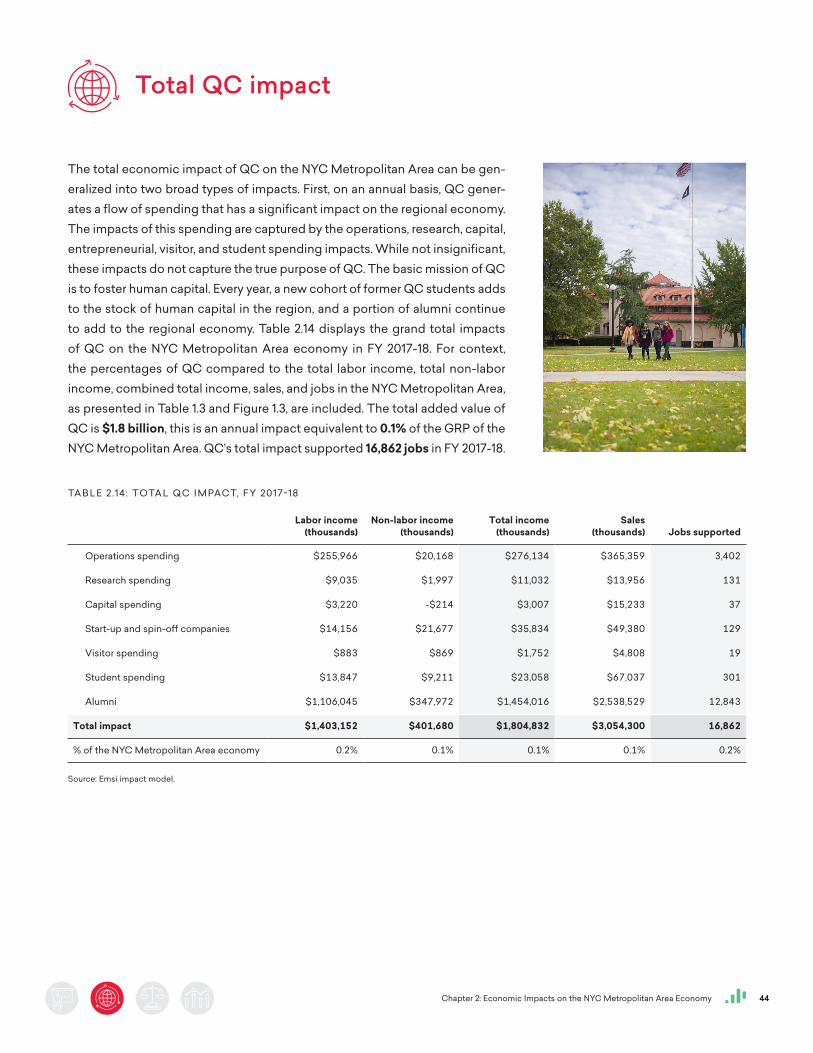
Chapter 2: Economic Impacts on the NYC Metropolitan Area Economy 44
Total QC impact
The total economic impact of QC on the NYC Metropolitan Area can be gen-eralized into two broad types of impacts. First, on an annual basis, QC gener-ates a flow of spending that has a significant impact on the regional economy. The impacts of this spending are captured by the operations, research, capital, entrepreneurial, visitor, and student spending impacts. While not insignificant, these impacts do not capture the true purpose of QC. The basic mission of QC is to foster human capital. Every year, a new cohort of former QC students adds to the stock of human capital in the region, and a portion of alumni continue to add to the regional economy. Table 2.14 displays the grand total impacts of QC on the NYC Metropolitan Area economy in FY 2017-18. For context, the percentages of QC compared to the total labor income, total non-labor income, combined total income, sales, and jobs in the NYC Metropolitan Area, as presented in Table 1.3 and Figure 1.3, are included. The total added value of QC is $1.8 billion, this is an annual impact equivalent to 0.1% of the GRP of the NYC Metropolitan Area. QC’s total impact supported 16,862 jobs in FY 2017-18.
TA B L E 2.14: TOTA L Q C I M PAC T, F Y 2017-18
Labor income
(thousands)Non-labor income
(thousands)Total income
(thousands)Sales
(thousands) Jobs supported
Operations spending $255,966 $20,168 $276,134 $365,359 3,402
Research spending $9,035 $1,997 $11,032 $13,956 131
Capital spending $3,220 -$214 $3,007 $15,233 37
Start-up and spin-off companies $14,156 $21,677 $35,834 $49,380 129
Visitor spending $883 $869 $1,752 $4,808 19
Student spending $13,847 $9,211 $23,058 $67,037 301
Alumni $1,106,045 $347,972 $1,454,016 $2,538,529 12,843
Total impact $1,403,152 $401,680 $1,804,832 $3,054,300 16,862
% of the NYC Metropolitan Area economy 0.2% 0.1% 0.1% 0.1% 0.2%
Source: Emsi impact model.
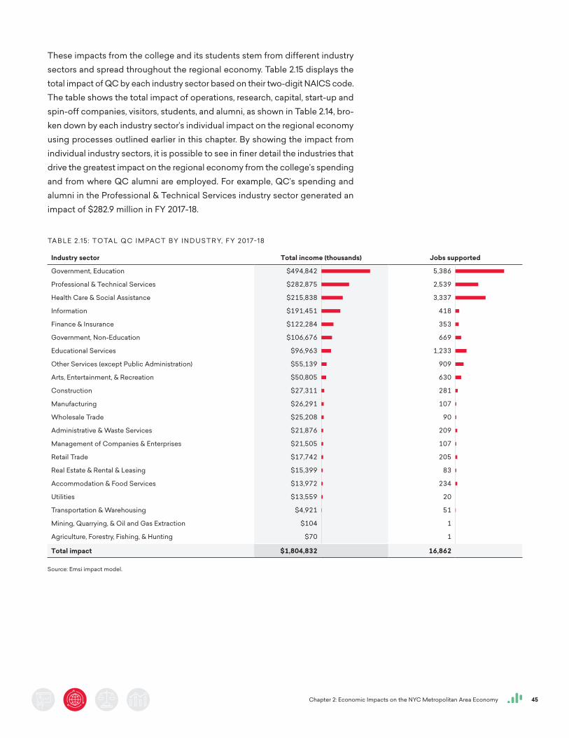
Chapter 2: Economic Impacts on the NYC Metropolitan Area Economy 45
These impacts from the college and its students stem from different industry sectors and spread throughout the regional economy. Table 2.15 displays the total impact of QC by each industry sector based on their two-digit NAICS code. The table shows the total impact of operations, research, capital, start-up and spin-off companies, visitors, students, and alumni, as shown in Table 2.14, bro-ken down by each industry sector’s individual impact on the regional economy using processes outlined earlier in this chapter. By showing the impact from individual industry sectors, it is possible to see in finer detail the industries that drive the greatest impact on the regional economy from the college’s spending and from where QC alumni are employed. For example, QC’s spending and alumni in the Professional & Technical Services industry sector generated an impact of $282.9 million in FY 2017-18.
TA B L E 2.15 : TOTA L Q C I M PAC T BY I N D U S T R Y, F Y 2017-18
Industry sector Total income (thousands) Jobs supported
Government, Education $494,842 5,386
Professional & Technical Services $282,875 2,539
Health Care & Social Assistance $215,838 3,337
Information $191,451 418
Finance & Insurance $122,284 353
Government, Non-Education $106,676 669
Educational Services $96,963 1,233
Other Services (except Public Administration) $55,139 909
Arts, Entertainment, & Recreation $50,805 630
Construction $27,311 281
Manufacturing $26,291 107
Wholesale Trade $25,208 90
Administrative & Waste Services $21,876 209
Management of Companies & Enterprises $21,505 107
Retail Trade $17,742 205
Real Estate & Rental & Leasing $15,399 83
Accommodation & Food Services $13,972 234
Utilities $13,559 20
Transportation & Warehousing $4,921 51
Mining, Quarrying, & Oil and Gas Extraction $104 1
Agriculture, Forestry, Fishing, & Hunting $70 1
Total impact $1,804,832 16,862
Source: Emsi impact model.
100+57+44+39+25+22+20+11+10+6+5+5+4+4+4+3+3+3+1+0+0
100+47+62+8+7+12+23+17+12+5+2+2+4+2+4+2+4+0+1+0+0
Chapter 3: Investment Analysis 46
C H A P T E R 3 :
Investment Analysis
The benefits generated by QC affect the lives of many people. The most obvious beneficiaries are the college’s students; they give up time and money to go to the college in return for a lifetime of higher wages and improved quality of life. But the benefits do not stop there. As
students earn more, communities and citizens throughout New York benefit from an enlarged economy and a reduced demand for social services. In the form of increased tax revenues and
public sector savings, the benefits of education extend as far as the state and local government.
Investment analysis is the process of evaluating total costs and measuring these against total benefits to determine whether or not a proposed venture will be profitable. If benefits outweigh
costs, then the investment is worthwhile. If costs outweigh benefits, then the investment will lose money and is thus considered infeasible. In this chapter, we consider QC as a
worthwhile investment from the perspectives of students, taxpayers, and society.
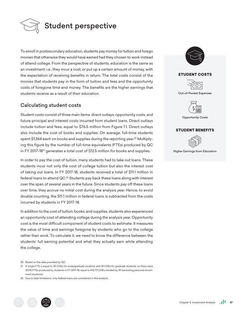
Chapter 3: Investment Analysis 47
Student perspective
To enroll in postsecondary education, students pay money for tuition and forego monies that otherwise they would have earned had they chosen to work instead of attend college. From the perspective of students, education is the same as an investment; i.e., they incur a cost, or put up a certain amount of money, with the expectation of receiving benefits in return. The total costs consist of the monies that students pay in the form of tuition and fees and the opportunity costs of foregone time and money. The benefits are the higher earnings that students receive as a result of their education.
Calculating student costs
Student costs consist of three main items: direct outlays, opportunity costs, and future principal and interest costs incurred from student loans. Direct outlays include tuition and fees, equal to $76.5 million from Figure 1.1. Direct outlays also include the cost of books and supplies. On average, full-time students spent $1,364 each on books and supplies during the reporting year.30 Multiply-ing this figure by the number of full-time equivalents (FTEs) produced by QC in FY 2017-1831 generates a total cost of $12.5 million for books and supplies.
In order to pay the cost of tuition, many students had to take out loans. These students incur not only the cost of college tuition but also the interest cost of taking out loans. In FY 2017-18, students received a total of $11.1 million in federal loans to attend QC.32 Students pay back these loans along with interest over the span of several years in the future. Since students pay off these loans over time, they accrue no initial cost during the analysis year. Hence, to avoid double counting, the $11.1 million in federal loans is subtracted from the costs incurred by students in FY 2017-18.
In addition to the cost of tuition, books, and supplies, students also experienced an opportunity cost of attending college during the analysis year. Opportunity cost is the most difficult component of student costs to estimate. It measures the value of time and earnings foregone by students who go to the college rather than work. To calculate it, we need to know the difference between the students’ full earning potential and what they actually earn while attending the college.
30 Based on the data provided by QC.31 A single FTE is equal to 30 CHEs for undergraduate students and 24 CHEs for graduate students, so there were
13,910 FTEs produced by students in FY 2017-18, equal to 413,771 CHEs divided by 30 (excluding personal enrich-ment students).
32 Due to data limitations, only federal loans are considered in this analysis.
Opportunity Costs
Higher Earnings from Education
Out-of-Pocket Expenses
STUDENT COSTS
STUDENT BENEFITS
Chapter 3: Investment Analysis 48
We derive the students’ full earning potential by weighting the average annual earnings levels in Table 1.4 according to the education level breakdown of the student population at first enrollment.33 However, the earnings levels in Table 1.4 reflect what average workers earn at the midpoint of their careers, not while attending the college. Because of this, we adjust the earnings levels to the average age of the student population (24) to better reflect their wages at their current age.34 This calculation yields an average full earning potential of $25,167 per student.
In determining how much students earn while enrolled in postsecondary education, an important factor to consider is the time that they actually spend on postsecondary education, since this is the only time that they are required to give up a portion of their earnings. We use the students’ CHE production as a proxy for time, under the assumption that the more CHEs students earn, the less time they have to work, and, consequently, the greater their foregone earnings. Overall, students attending QC earned an average of 15.5 CHEs per student (excluding personal enrichment students and dual-credit high school students), which is approximately equal to 55% of a full academic year.35 We thus include no more than $13,772 (or 55%) of the students’ full earning potential in the opportunity cost calculations.
Another factor to consider is the students’ employment status while enrolled in postsecondary education. It is estimated that 58% of students are employed.36 For the remainder of students, we assume that they are either seeking work or planning to seek work once they complete their educational goals (with the exception of personal enrichment students, who are not included in this calculation). By choosing to enroll, therefore, non-working students give up everything that they can potentially earn during the academic year (i.e., the $13,772). The total value of their foregone earnings thus comes to $151.5 million.
Working students are able to maintain all or part of their earnings while enrolled. However, many of them hold jobs that pay less than statistical averages, usually because those are the only jobs they can find that accommodate their course schedule. These jobs tend to be at entry level, such as restaurant servers or cashiers. To account for this, we assume that working students hold jobs that pay 73% of what they would have earned had they chosen to work full-time rather than go to college.37 The remaining 27% comprises the percentage of
33 This is based on students who reported their prior level of education to QC. The prior level of education data was then adjusted to exclude dual credit high school students.
34 Further discussion on this adjustment appears in Appendix 6.35 Equal to 15.5 CHEs divided by 30 for the proportion of undergraduate students and 24 for the proportion of gradu-
ate students, the assumed number of CHEs in a full-time academic year.36 Based on data provided by QC. This figure excludes dual credit high school students, who are not included in
the opportunity cost calculations.37 The 73% assumption is based on the average hourly wage of jobs commonly held by working students divided by
the national average hourly wage. Occupational wage estimates are published by the Bureau of Labor Statistics (see http://www.bls.gov/oes/current/oes_nat.htm).
Chapter 3: Investment Analysis 49
their full earning potential that they forego. Obviously this assumption varies by person; some students forego more and others less. Since we do not know the actual jobs that students hold while attending, the 27% in foregone earn-ings serves as a reasonable average.
Working students also give up a portion of their leisure time in order to attend higher education institutions. According to the Bureau of Labor Statistics American Time Use Survey, students forego up to 0.5 hours of leisure time per day.38 Assuming that an hour of leisure is equal in value to an hour of work, we derive the total cost of leisure by multiplying the number of leisure hours foregone during the academic year by the average hourly pay of the students’ full earning potential. For working students, therefore, their total opportunity cost is $70.1 million, equal to the sum of their foregone earnings ($56.2 million) and foregone leisure time ($13.9 million).
Thus far we have discussed student costs during the analysis year. However, recall that students take out student loans to attend college during the year, which they will have to pay back over time. The amount they will be paying in the future must be a part of their decision to attend the college today. Stu-dents who take out loans are required not only to pay back the principal of the loan but also to pay a certain amount in interest. The first step in calculating students’ loan interest cost is to determine the payback time for the loans. The $11.1 million in loans was awarded to 1,854 students, averaging $5,968 per student in the analysis year. However, this figure represents only one year of loans. Because loan payback time is determined by total indebtedness, and QC is a four-year college, we assume that students will be indebted four times that amount, or $23,870 on average. According to the U.S. Department of Education, this level of indebtedness will take 20 years to pay back under the standard repayment plan.39
This indebtedness calculation is used solely to estimate the loan payback period. Students will be paying back the principal amount of $11.1 million over time. After taking into consideration the time value of money, this means that students will pay off a discounted present value of $6.8 million in principal over the 20 years. In order to calculate interest, we only consider interest on the federal loans awarded to students in FY 2017-18. Using the student discount rate of 4.5%40 as our interest rate, we calculate that students will pay a total discounted present value of $4.1 million in interest on student loans throughout
38 “Charts by Topic: Leisure and Sports Activities,” American Time Use Survey, Last modified December 2016. http://www.bls.gov/tus/charts/leisure.htm.
39 Repayment period based on total education loan indebtedness, U.S. Department of Education, 2017. https://studentaid.ed.gov/sa/repay-loans/understand/plans/standard.
40 The student discount rate is derived from the baseline forecasts for the 10-year discount rate published by the Congressional Budget Office. See the Congressional Budget Office, Student Loan and Pell Grant Programs – April 2018 Baseline. https://www.cbo.gov/system/files?file=2018-06/51310-2018-04-studentloan.pdf.
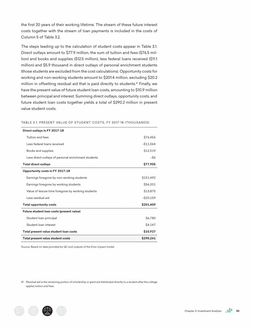
Chapter 3: Investment Analysis 50
the first 20 years of their working lifetime. The stream of these future interest costs together with the stream of loan payments is included in the costs of Column 5 of Table 3.2.
The steps leading up to the calculation of student costs appear in Table 3.1. Direct outlays amount to $77.9 million, the sum of tuition and fees ($76.5 mil-lion) and books and supplies ($12.5 million), less federal loans received ($11.1 million) and $5.9 thousand in direct outlays of personal enrichment students (those students are excluded from the cost calculations). Opportunity costs for working and non-working students amount to $201.4 million, excluding $20.2 million in offsetting residual aid that is paid directly to students.41 Finally, we have the present value of future student loan costs, amounting to $10.9 million between principal and interest. Summing direct outlays, opportunity costs, and future student loan costs together yields a total of $290.2 million in present value student costs.
41 Residual aid is the remaining portion of scholarship or grant aid distributed directly to a student after the college applies tuition and fees.
TA B L E 3.1 : P R E S E N T VA L U E O F S T U D E N T C O S T S, F Y 2017-18 ( T H O U SA N D S)
Direct outlays in FY 2017-18
Tuition and fees $76,456
Less federal loans received -$11,064
Books and supplies $12,519
Less direct outlays of personal enrichment students -$6
Total direct outlays $77,905
Opportunity costs in FY 2017-18
Earnings foregone by non-working students $151,492
Earnings foregone by working students $56,201
Value of leisure time foregone by working students $13,875
Less residual aid -$20,159
Total opportunity costs $201,409
Future student loan costs (present value)
Student loan principal $6,780
Student loan interest $4,147
Total present value student loan costs $10,927
Total present value student costs $290,241
Source: Based on data provided by QC and outputs of the Emsi impact model.
Chapter 3: Investment Analysis 51
Linking education to earnings
Having estimated the costs of education to students, we weigh these costs against the benefits that students receive in return. The relationship between education and earnings is well documented and forms the basis for determin-ing student benefits. As shown in Table 1.4, state mean earnings levels at the midpoint of the average-aged worker’s career increase as people achieve higher levels of education. The differences between state earnings levels define the incremental benefits of moving from one education level to the next.
A key component in determining the students’ return on investment is the value of their future benefits stream; i.e., what they can expect to earn in return for the investment they make in education. We calculate the future benefits stream to the college’s FY 2017-18 students first by determining their average annual increase in earnings, equal to $103.1 million. This value represents the higher wages that accrue to students at the midpoint of their careers and is calculated based on the marginal wage increases of the CHEs that students complete while attending the college. Using New York State earnings, the marginal wage increase per CHE is $249. For a full description of the methodology used to derive the $103.1 million, see Appendix 6.
The second step is to project the $103.1 million annual increase in earnings into the future, for as long as students remain in the workforce. We do this using the Mincer function to predict the change in earnings at each point in an individual’s working career.42 The Mincer function originated from Mincer’s seminal work on human capital (1958). The function estimates earnings using an individual’s years of education and post-schooling experience. While some have criticized Mincer’s earnings function, it is still upheld in recent data and has served as the foundation for a variety of research pertaining to labor economics. Card (1999 and 2001) addresses a number of these criticisms using U.S.-based research over the last three decades and concludes that any upward bias in the Mincer parameters is on the order of 10% or less. We use state-specific and education level-specific Mincer coefficients. To account for any upward bias, we incorpo-rate a 10% reduction in our projected earnings, otherwise known as the ability bias. With the $103.1 million representing the students’ higher earnings at the midpoint of their careers, we apply scalars from the Mincer function to yield a stream of projected future benefits that gradually increase from the time students enter the workforce, peak shortly after the career midpoint, and then dampen slightly as students approach retirement at age 67, the full retirement age in the US. This earnings stream appears in Column 2 of Table 3.2.
42 Appendix 6 provides more information on the Mincer function and how it is used to predict future earnings growth.
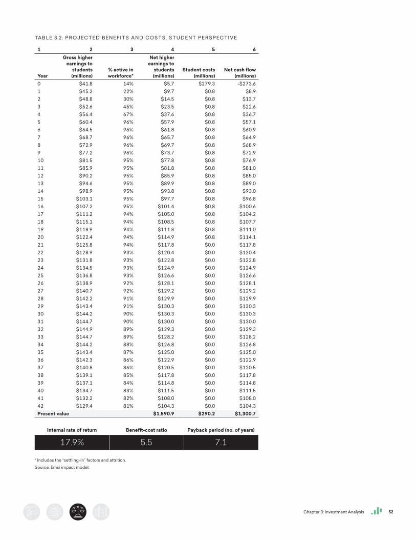
Chapter 3: Investment Analysis 52
TA B L E 3.2 : P R O J E C T E D B E N E F I T S A N D C O S T S, S T U D E N T P E R S P E C T I V E
1 2 3 4 5 6
Year
Gross higher earnings to
students(millions)
% active in workforce*
Net higher earnings to
students(millions)
Student costs(millions)
Net cash flow(millions)
0 $41.8 14% $5.7 $279.3 -$273.61 $45.2 22% $9.7 $0.8 $8.92 $48.8 30% $14.5 $0.8 $13.73 $52.6 45% $23.5 $0.8 $22.64 $56.4 67% $37.6 $0.8 $36.75 $60.4 96% $57.9 $0.8 $57.16 $64.5 96% $61.8 $0.8 $60.97 $68.7 96% $65.7 $0.8 $64.98 $72.9 96% $69.7 $0.8 $68.99 $77.2 96% $73.7 $0.8 $72.910 $81.5 95% $77.8 $0.8 $76.911 $85.9 95% $81.8 $0.8 $81.012 $90.2 95% $85.9 $0.8 $85.013 $94.6 95% $89.9 $0.8 $89.014 $98.9 95% $93.8 $0.8 $93.015 $103.1 95% $97.7 $0.8 $96.816 $107.2 95% $101.4 $0.8 $100.617 $111.2 94% $105.0 $0.8 $104.218 $115.1 94% $108.5 $0.8 $107.719 $118.9 94% $111.8 $0.8 $111.020 $122.4 94% $114.9 $0.8 $114.121 $125.8 94% $117.8 $0.0 $117.822 $128.9 93% $120.4 $0.0 $120.423 $131.8 93% $122.8 $0.0 $122.824 $134.5 93% $124.9 $0.0 $124.925 $136.8 93% $126.6 $0.0 $126.626 $138.9 92% $128.1 $0.0 $128.127 $140.7 92% $129.2 $0.0 $129.228 $142.2 91% $129.9 $0.0 $129.929 $143.4 91% $130.3 $0.0 $130.330 $144.2 90% $130.3 $0.0 $130.331 $144.7 90% $130.0 $0.0 $130.032 $144.9 89% $129.3 $0.0 $129.333 $144.7 89% $128.2 $0.0 $128.234 $144.2 88% $126.8 $0.0 $126.835 $143.4 87% $125.0 $0.0 $125.036 $142.3 86% $122.9 $0.0 $122.937 $140.8 86% $120.5 $0.0 $120.538 $139.1 85% $117.8 $0.0 $117.839 $137.1 84% $114.8 $0.0 $114.840 $134.7 83% $111.5 $0.0 $111.541 $132.2 82% $108.0 $0.0 $108.042 $129.4 81% $104.3 $0.0 $104.3Present value $1,590.9 $290.2 $1,300.7
Internal rate of return Benefit-cost ratio Payback period (no. of years)
17.9% 5.5 7.1
* Includes the “settling-in” factors and attrition.
Source: Emsi impact model.
Chapter 3: Investment Analysis 53
As shown in Table 3.2, the $103.1 million in gross higher earnings occurs around Year 15, which is the approximate midpoint of the students’ future working careers given the average age of the student population and an assumed retirement age of 67. In accordance with the Mincer function, the gross higher earnings that accrue to students in the years leading up to the midpoint are less than $103.1 million and the gross higher earnings in the years after the midpoint are greater than $103.1 million.
The final step in calculating the students’ future benefits stream is to net out the potential benefits generated by students who are either not yet active in the workforce or who leave the workforce over time. This adjustment appears in Column 3 of Table 3.2 and represents the percentage of the FY 2017-18 student population that will be employed in the workforce in a given year. Note that the percentages in the first five years of the time horizon are relatively lower than those in subsequent years. This is because many students delay their entry into the workforce, either because they are still enrolled at the college or because they are unable to find a job immediately upon graduation. Accordingly, we apply a set of “settling-in” factors to account for the time needed by students to find employment and settle into their careers. As discussed in Chapter 2, settling-in factors delay the onset of the benefits by one to three years for students who graduate with a certificate or a degree and by one to five years for degree-seeking students who do not graduate during the analysis year.
Beyond the first five years of the time horizon, students will leave the workforce for any number of reasons, whether death, retirement, or unemployment. We estimate the rate of attrition using the same data and assumptions applied in the calculation of the attrition rate in the economic impact analysis of Chapter 2.43 The likelihood of leaving the workforce increases as students age, so the attrition rate is more aggressive near the end of the time horizon than in the beginning. Column 4 of Table 3.2 shows the net higher earnings to students after accounting for both the settling-in patterns and attrition.
Return on investment for students
Having estimated the students’ costs and their future benefits stream, the next step is to discount the results to the present to reflect the time value of money. For the student perspective we assume a discount rate of 4.5% (see below). Because students tend to rely upon debt to pay for education—i.e. they are negative savers—their discount rate is based upon student loan interest rates.44
43 See the discussion of the alumni impact in Chapter 2. The main sources for deriving the attrition rate are the National Center for Health Statistics, the Social Security Administration, and the Bureau of Labor Statistics. Note that we do not account for migration patterns in the student investment analysis because the higher earnings that students receive as a result of their education will accrue to them regardless of where they find employment.
44 The student discount rate is derived from the baseline forecasts for the 10-year Treasury rate published by the Congressional Budget Office. See the Congressional Budget Office, Student Loan and Pell Grant Programs – April 2018 Baseline. https://www.cbo.gov/system/files?file=2018-06/51310-2018-04-studentloan.pdf.
Discount rate
The discount rate is a rate of interest that converts future costs and benefits to present values. For example, $1,000 in higher earnings realized 30 years in the future is worth much less than $1,000 in the present. All future values must therefore be expressed in present value terms in order to compare them with investments (i.e., costs) made today. The selection of an appropriate discount rate, however, can become an arbitrary and controversial undertaking. As suggested in economic theory, the discount rate should reflect the inves-tor’s opportunity cost of capital, i.e., the rate of return one could reasonably expect to obtain from alternative invest-ment schemes. In this study we assume a 4.5% discount rate from the student perspective and a 1.0% discount rate from the perspectives of taxpayers and society.
Chapter 3: Investment Analysis 54
In Appendix 1, we conduct a sensitivity analysis of this discount rate. The present value of the benefits is then compared to student costs to derive the invest-ment analysis results, expressed in terms of a benefit-cost ratio, rate of return, and payback period. The investment is feasible if returns match or exceed the minimum threshold values; i.e., a benefit-cost ratio greater than 1.0, a rate of return that exceeds the discount rate, and a reasonably short payback period.
In Table 3.2, the net higher earnings of students yield a cumulative discounted sum of approximately $1.6 billion, the present value of all of the future earnings increments (see the bottom section of Column 4). This may also be interpreted as the gross capital asset value of the students’ higher earnings stream. In effect, the aggregate FY 2017-18 student body is rewarded for its investment in QC with a capital asset valued at $1.6 billion.
The students’ cost of attending the college is shown in Column 5 of Table 3.2, equal to a present value of $290.2 million. Comparing the cost with the present value of benefits yields a student benefit-cost ratio of 5.5 (equal to $1.6 billion in benefits divided by $290.2 million in costs).
Another way to compare the same benefits stream and associated cost is to compute the rate of return. The rate of return indicates the interest rate that a bank would have to pay a depositor to yield an equally attractive stream of future payments.45 Table 3.2 shows QC stu-dents earning average returns of 17.9% on their invest-ment of time and money. This is a favorable return compared, for example, to approximately 1% on a standard bank savings account, or 10% on stocks and bonds (30-year average return).
Note that returns reported in this study are real returns, not nominal. When a bank promises to pay a certain rate of interest on a savings account, it employs an implicitly nominal rate. Bonds operate in a similar manner. If it turns out that the inflation rate is higher than the stated rate of return, then money is lost in real terms. In contrast, a real rate of return is on top of inflation. For example, if inflation is running at 3% and a nominal percentage of 5% is paid, then the real rate of return on the investment is only 2%. In Table 3.2, the 17.9% student rate of return is a real rate. With an inflation rate of 2.2% (the average rate reported over the past 20 years as per the U.S. Department of Commerce, Consumer
45 Rates of return are computed using the familiar internal rate-of-return calculation. Note that with a bank deposit or stock market investment, the depositor puts up a principal, receives in return a stream of periodic payments, and then recovers the principal at the end. Someone who invests in education, on the other hand, receives a stream of periodic payments that include the recovery of the principal as part of the periodic payments, but there is no principal recovery at the end. These differences notwithstanding, comparable cash flows for both bank and education investors yield the same internal rate of return.
QC students see an average rate of return of 17.9% for their investment of time and money.
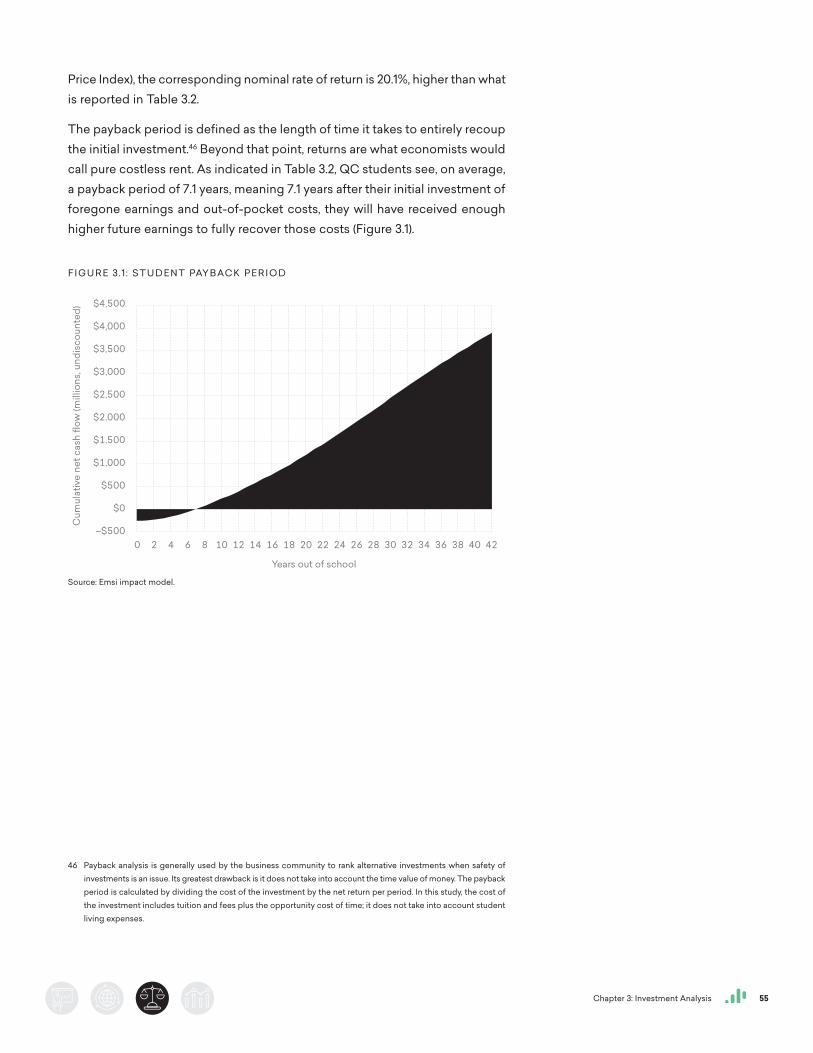
Chapter 3: Investment Analysis 55
Price Index), the corresponding nominal rate of return is 20.1%, higher than what is reported in Table 3.2.
The payback period is defined as the length of time it takes to entirely recoup the initial investment.46 Beyond that point, returns are what economists would call pure costless rent. As indicated in Table 3.2, QC students see, on average, a payback period of 7.1 years, meaning 7.1 years after their initial investment of foregone earnings and out-of-pocket costs, they will have received enough higher future earnings to fully recover those costs (Figure 3.1).
46 Payback analysis is generally used by the business community to rank alternative investments when safety of investments is an issue. Its greatest drawback is it does not take into account the time value of money. The payback period is calculated by dividing the cost of the investment by the net return per period. In this study, the cost of the investment includes tuition and fees plus the opportunity cost of time; it does not take into account student living expenses.
F I G U R E 3.1 : S T U D E N T PAY BAC K P E R I O D
Source: Emsi impact model.
Cum
ulat
ive
net c
ash
flow
(mill
ions
, und
isco
unte
d)
Years out of school
0 4 8 12 16 20 24 4228 32 36 40383430262218141062
$4,500
$2,500
$2,000
$1,500
$1,000
$500
$0
–$500
$3,000
$3,500
$4,000
Chapter 3: Investment Analysis 56
Taxpayer perspective
From the taxpayer perspective, the pivotal step is to determine the public benefits that specifically accrue to state and local government. For example, benefits resulting from earnings growth are limited to increased state and local tax payments. Similarly, savings related to improved health, reduced crime, and fewer welfare and unemployment claims, discussed below, are limited to those received strictly by state and local government. In all instances, benefits to private residents, local businesses, or the federal government are excluded.
Growth in state tax revenues
As a result of their time at QC, students earn more because of the skills they learned while attending the college, and businesses earn more because stu-dent skills make capital more productive (buildings, machinery, and everything else). This in turn raises profits and other business property income. Together, increases in labor and non-labor (i.e., capital) income are considered the effect of a skilled workforce. These in turn increase tax revenues since state and local government is able to apply tax rates to higher earnings.
Estimating the effect of QC on increased tax revenues begins with the present value of the students’ future earnings stream, which is displayed in Column 4 of Table 3.2. To these net higher earnings, we apply a multiplier derived from Emsi’s MR-SAM model to estimate the added labor income created in the state as students and businesses spend their higher earnings.47 As labor income increases, so does non-labor income, which consists of monies gained through investments. To calculate the growth in non-labor income, we multiply the increase in labor income by a ratio of the gross New York State product to total labor income in the state. We also include the spending impacts discussed in Chapter 2 that were created in FY 2017-18 from operations, research, capital, visitor, and student spending, measured at the state level. To each of these, we apply the prevailing tax rates so we capture only the tax revenues attributable to state and local government from this additional revenue.
Not all of these tax revenues may be counted as benefits to the state, however. Some students leave the state during the course of their careers, and the higher earnings they receive as a result of their education leave the state with them. To account for this dynamic, we combine student settlement data from the college with data on migration patterns from the Census Bureau to estimate the number of students who will leave the state workforce over time.
47 For a full description of the Emsi MR-SAM model, see Appendix 5.
Increased Tax Revenue
Avoided Costs to State/Local Government
State/Local Funding
TAXPAYER COSTS
TAXPAYER BENEFITS
Chapter 3: Investment Analysis 57
We apply another reduction factor to account for the students’ alternative education opportunities. This is the same adjustment that we use in the cal-culation of the alumni impact in Chapter 2 and is designed to account for the counterfactual scenario where QC does not exist. The assumption in this case is that any benefits generated by students who could have received an educa-tion even without the college cannot be counted as new benefits to society. For this analysis, we assume an alternative education variable of 15%, meaning that 15% of the student population at the college would have generated ben-efits anyway even without the college. For more information on the alternative education variable, see Appendix 7.
We apply a final adjustment factor to account for the “shutdown point” that nets out benefits that are not directly linked to the state and local government costs of supporting the college. As with the alternative education variable dis-cussed under the alumni impact, the purpose of this adjustment is to account for counterfactual scenarios. In this case, the counterfactual scenario is where state and local government funding for QC did not exist and QC had to derive the revenue elsewhere. To estimate this shutdown point, we apply a sub-model that simulates the students’ demand curve for education by reducing state and local support to zero and progressively increasing student tuition and fees. In our model, as student tuition and fees increase, enrollment declines, all other factors held constant. For QC, the shutdown point adjustment is 0%, meaning that the college could not operate without taxpayer support. As such, no reduc-tion applies. For more information on the theory and methodology behind the estimation of the shutdown point, see Appendix 9.
After adjusting for attrition, alternative education opportunities, and the shut-down point, we calculate the present value of the future added tax revenues that occur in the state, equal to $509.3 million. Recall from the discussion of the student return on investment that the present value represents the sum of the future benefits that accrue each year over the course of the time horizon, discounted to current year dollars to account for the time value of money. Given that the stakeholder in this case is the public sector, we use the discount rate of 1.0%. This is the real treasury interest rate recommended by the Office of Management and Budget (OMB) for 30-year investments, and in Appendix 1, we conduct a sensitivity analysis of this discount rate. 48
Government savings
In addition to the creation of higher tax revenues to the state and local govern-ment, education is statistically associated with a variety of lifestyle changes
48 Office of Management and Budget. “Discount Rates for Cost-Effectiveness Analysis of Federal Programs.” Real Interest Rates on Treasury Notes and Bonds of Specified Maturities (in Percent). Last modified November 2018. https://www.whitehouse.gov/wp-content/uploads/2018/12/Discount-History.pdf.
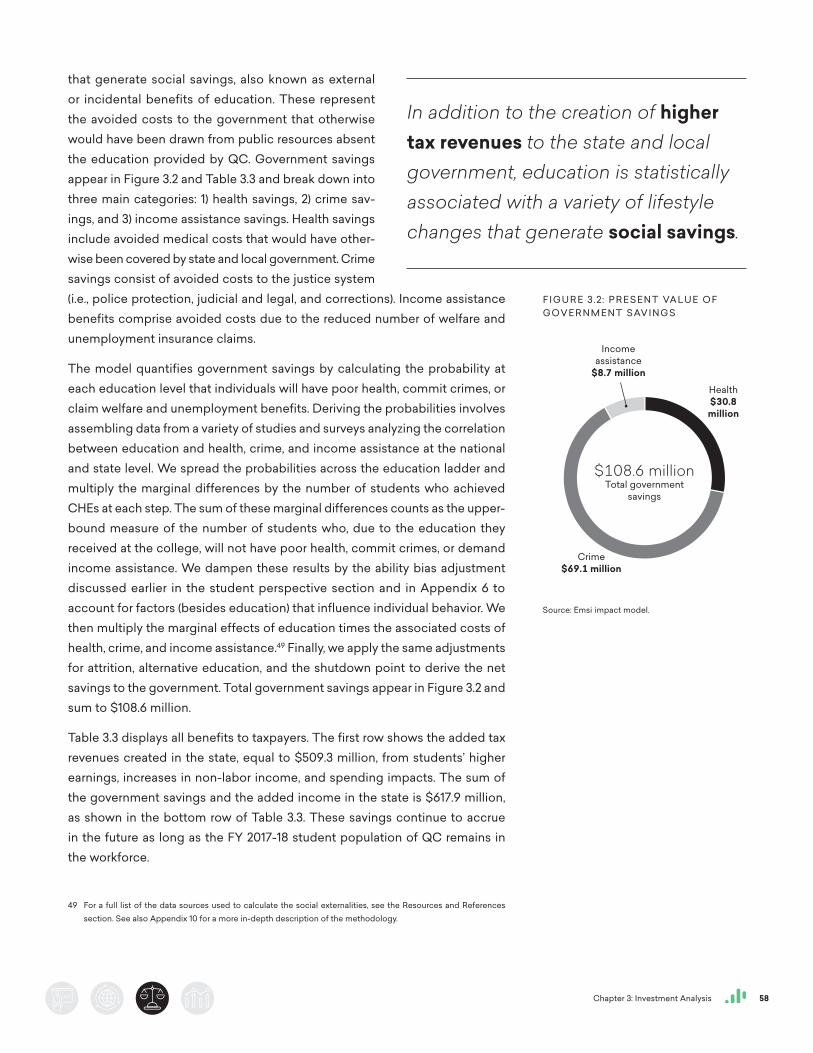
Chapter 3: Investment Analysis 58
that generate social savings, also known as external or incidental benefits of education. These represent the avoided costs to the government that otherwise would have been drawn from public resources absent the education provided by QC. Government savings appear in Figure 3.2 and Table 3.3 and break down into three main categories: 1) health savings, 2) crime sav-ings, and 3) income assistance savings. Health savings include avoided medical costs that would have other-wise been covered by state and local government. Crime savings consist of avoided costs to the justice system (i.e., police protection, judicial and legal, and corrections). Income assistance benefits comprise avoided costs due to the reduced number of welfare and unemployment insurance claims.
The model quantifies government savings by calculating the probability at each education level that individuals will have poor health, commit crimes, or claim welfare and unemployment benefits. Deriving the probabilities involves assembling data from a variety of studies and surveys analyzing the correlation between education and health, crime, and income assistance at the national and state level. We spread the probabilities across the education ladder and multiply the marginal differences by the number of students who achieved CHEs at each step. The sum of these marginal differences counts as the upper-bound measure of the number of students who, due to the education they received at the college, will not have poor health, commit crimes, or demand income assistance. We dampen these results by the ability bias adjustment discussed earlier in the student perspective section and in Appendix 6 to account for factors (besides education) that influence individual behavior. We then multiply the marginal effects of education times the associated costs of health, crime, and income assistance.49 Finally, we apply the same adjustments for attrition, alternative education, and the shutdown point to derive the net savings to the government. Total government savings appear in Figure 3.2 and sum to $108.6 million.
Table 3.3 displays all benefits to taxpayers. The first row shows the added tax revenues created in the state, equal to $509.3 million, from students’ higher earnings, increases in non-labor income, and spending impacts. The sum of the government savings and the added income in the state is $617.9 million, as shown in the bottom row of Table 3.3. These savings continue to accrue in the future as long as the FY 2017-18 student population of QC remains in the workforce.
49 For a full list of the data sources used to calculate the social externalities, see the Resources and References section. See also Appendix 10 for a more in-depth description of the methodology.
F I G U R E 3.2 : P R E S E N T VA L U E O F G OV E R N M E N T SAV I N G S
Source: Emsi impact model.
2828+6464+88+RHealth$30.8
million
Crime$69.1 million
Income assistance
$8.7 million
In addition to the creation of higher tax revenues to the state and local government, education is statistically associated with a variety of lifestyle changes that generate social savings.
$108.6 millionTotal government
savings
Chapter 3: Investment Analysis 59
Return on investment for taxpayers
Taxpayer costs are reported in Table 3.4 and come to $127 million, equal to the contribution of state and local government to QC. In return for their public support, taxpayers are rewarded with an investment benefit-cost ratio of 4.9 (= $617.9 million ÷ $127 million), indicating a profitable investment.
At 13.3%, the rate of return to state and local taxpayers is favorable. Given that the stakeholder in this case is the public sector, we use the discount rate of 1.0%, the real treasury interest rate recommended by the Office of Management and Budget for 30-year investments.50 This is the return governments are assumed to be able to earn on generally safe investments of unused funds, or alternatively, the interest rate for which governments, as relatively safe borrowers, can obtain funds. A rate of return of 1.0% would mean that the college just pays its own way. In principle, govern-ments could borrow monies used to support QC and repay the loans out of the resulting added taxes and reduced government expenditures. A rate of return of 13.3%, on the other hand, means that QC not only pays its own way, but also generates a surplus that the state and local government can use to fund other programs. It is unlikely that other government programs could make such a claim.
50 Office of Management and Budget. “Discount Rates for Cost-Effectiveness Analysis of Federal Programs.” Real Interest Rates on Treasury Notes and Bonds of Specified Maturities (in Percent). Last modified November 2018. https://www.whitehouse.gov/wp-content/uploads/2018/12/Discount-History.pdf.
TA B L E 3.3 : P R E S E N T VA L U E O F A D D E D TA X R E V E N U E A N D G OV E R N M E N T SAV I N G S ( T H O U SA N D S)
Added tax revenue $509,296
Government savings
Health-related savings $30,773
Crime-related savings $69,145
Income assistance savings $8,728
Total government savings $108,646
Total taxpayer benefits $617,942
Source: Emsi impact model.
A rate of return of 13.3% means that QC not only pays its own way, but also generates a surplus that the state and local government can use to fund other programs.
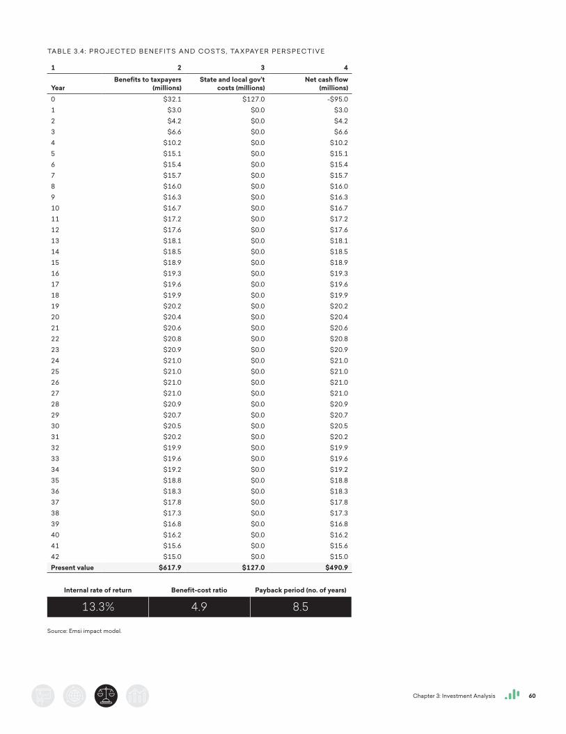
Chapter 3: Investment Analysis 60
TA B L E 3.4: P R O J E C T E D B E N E F I T S A N D C O S T S, TA X PAY E R P E R S P E C T I V E
1 2 3 4
YearBenefits to taxpayers
(millions)State and local gov’t
costs (millions)Net cash flow
(millions)0 $32.1 $127.0 -$95.01 $3.0 $0.0 $3.02 $4.2 $0.0 $4.23 $6.6 $0.0 $6.64 $10.2 $0.0 $10.25 $15.1 $0.0 $15.16 $15.4 $0.0 $15.47 $15.7 $0.0 $15.78 $16.0 $0.0 $16.09 $16.3 $0.0 $16.310 $16.7 $0.0 $16.711 $17.2 $0.0 $17.212 $17.6 $0.0 $17.613 $18.1 $0.0 $18.114 $18.5 $0.0 $18.515 $18.9 $0.0 $18.916 $19.3 $0.0 $19.317 $19.6 $0.0 $19.618 $19.9 $0.0 $19.919 $20.2 $0.0 $20.220 $20.4 $0.0 $20.421 $20.6 $0.0 $20.622 $20.8 $0.0 $20.823 $20.9 $0.0 $20.924 $21.0 $0.0 $21.025 $21.0 $0.0 $21.026 $21.0 $0.0 $21.027 $21.0 $0.0 $21.028 $20.9 $0.0 $20.929 $20.7 $0.0 $20.730 $20.5 $0.0 $20.531 $20.2 $0.0 $20.232 $19.9 $0.0 $19.933 $19.6 $0.0 $19.634 $19.2 $0.0 $19.235 $18.8 $0.0 $18.836 $18.3 $0.0 $18.337 $17.8 $0.0 $17.838 $17.3 $0.0 $17.339 $16.8 $0.0 $16.840 $16.2 $0.0 $16.241 $15.6 $0.0 $15.642 $15.0 $0.0 $15.0Present value $617.9 $127.0 $490.9
Internal rate of return Benefit-cost ratio Payback period (no. of years)
13.3% 4.9 8.5
Source: Emsi impact model.
Chapter 3: Investment Analysis 61
Social perspective
New York benefits from the education that QC provides through the earnings that students create in the state and through the savings that they generate through their improved lifestyles. QC ranked eleventh in 2018 and fourth in 2019 in College Net’s Social Mobility Index.51 The Social Mobility Index (SMI) measures the extent to which a college or university educates more economi-cally disadvantaged students (with family incomes below the national median) at lower tuition and graduates them into good-paying jobs. More evidence of QC’s realization for transforming its students’ lives through increased upward mobility is QC’s rank on the Mobility Report Cards: The Role of Colleges in Intergenerational Mobility.52
To receive these benefits, however, members of society must pay money and forego services that they otherwise would have enjoyed if QC did not exist. Society’s investment in QC stretches across a number of investor groups, from students to employers to taxpayers. We weigh the benefits generated by QC to these investor groups against the total social costs of generating those benefits. The total social costs include all QC expenditures, all student expenditures (including interest on student loans) less tuition and fees, and all student opportunity costs, totaling a present value of $517.2 million.
On the benefits side, any benefits that accrue to New York as a whole—including students, employers, taxpayers, and anyone else who stands to benefit from the activities of QC—are counted as benefits under the social perspective. We group these benefits under the following broad headings: 1) increased earnings in the state, and 2) social externalities stemming from improved health, reduced crime, and reduced unemployment in the state (see the Beekeeper Analogy box for a discussion of externalities). Both of these benefits components are described more fully in the following sections.
51 As cited in https://www.socialmobilityindex.org/52 As cited in https://opportunityinsights.org/wp-content/uploads/2018/03/coll_mrc_summary.pdf. The CUNY
System was ranked #6 in U.S. colleges that have the highest upward mobility rates.
Student Opportunity Costs
Student Out-of-Pocket Expenses
Increased State Earnings
Avoided Costs to Society
QC Expenditures
SOCIAL COSTS
SOCIAL BENEFITS
QC enhances community well-being
QC uses its facilities to support the diverse population of its home borough. Recent public events on the campus have included New York State’s first Veterans Resource Fair; a Black Business Expo that highlighted African American-owned companies and enabled their representatives to network with students; CUNY Pridefest, which included an LGBTQIA+ expo; and just last fall, the College Fair for Young Men, which attracted more than 2,000 high school students, most of them young men of color.
Chapter 3: Investment Analysis 62
Growth in state economic base
In the process of absorbing the newly acquired skills of students who attend QC, not only does the productivity of the New York workforce increase, but so does the productivity of its physical capital and assorted infrastructure. Students earn more because of the skills they learned while attending the college, and businesses earn more because student skills make capital more productive (buildings, machinery, and everything else). This in turn raises profits and other business property income. Together, increases in labor and non-labor (i.e., capital) income are considered the effect of a skilled workforce.
Estimating the effect of QC on the state’s economic base follows a similar pro-cess used when calculating increased tax revenues in the taxpayer perspective. However, instead of looking at just the tax revenue portion, we include all of the added earnings and business output. First, we calculate the students’ future higher-earnings stream. We factor in student attrition and alternative educa-tion opportunities to arrive at net higher earnings. We again apply multipliers derived from Emsi’s MR-SAM model to estimate the added labor and non-labor income created in the state as students and businesses spend their higher earnings and as businesses generate additional profits from this increased output. We also include the operations, research, capital, visitor, and student spending impacts discussed in Chapter 2 that were created in FY 2017-18, measured at the state level. The shutdown point does not apply to the growth of the economic base because the social perspective captures not only the state and local taxpayer support to the college, but also the support from the students and other non-government sources.
Using this process, we calculate the present value of the future added income that occurs in the state, equal to $4.9 billion. Recall from the discussion of the student and taxpayer return on investment that the present value represents the sum of the future benefits that accrue each year over the course of the time horizon, discounted to current year dollars to account for the time value of money. As stated in the taxpayer perspective, given that the stakeholder in this case is the public sector, we use the discount rate of 1.0%.
Social savings
Similar to the government savings discussed above, society as a whole sees savings due to external or incidental benefits of education. These represent the avoided costs that otherwise would have been drawn from private and public resources absent the education provided by QC. Social benefits appear in Table 3.5 and break down into three main categories: 1) health savings, 2) crime savings, and 3) income assistance savings. These are similar to the categories from the taxpayer perspective above, although health savings now also account for lost productivity and other effects associated with smoking, alcohol depen-
Beekeeper analogy
Beekeepers provide a classic example of positive externalities (sometimes called “neighborhood effects”). The beekeeper’s intention is to make money selling honey. Like any other business, receipts must at least cover operat-ing costs. If they don’t, the business shuts down.
But from society’s standpoint, there is more. Flowers provide the nectar that bees need for honey production, and smart beekeepers locate near flower-ing sources such as orchards. Nearby orchard owners, in turn, benefit as the bees spread the pollen necessary for orchard growth and fruit production. This is an uncompensated external benefit of beekeeping, and economists have long recognized that society might actually do well to subsidize activities that produce positive externalities, such as beekeeping.
Educational institutions are like bee-keepers. While their principal aim is to provide education and raise people’s earnings, in the process they create an array of external benefits. Students’ health and lifestyles are improved, and society indirectly benefits just as orchard owners indirectly benefit from beekeepers. Aiming at a more complete accounting of the benefits generated by education, the model tracks and accounts for many of these external social benefits.
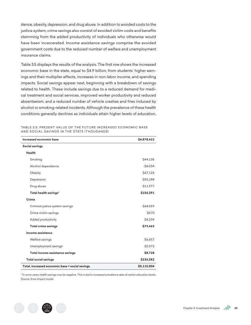
Chapter 3: Investment Analysis 63
dence, obesity, depression, and drug abuse. In addition to avoided costs to the justice system, crime savings also consist of avoided victim costs and benefits stemming from the added productivity of individuals who otherwise would have been incarcerated. Income assistance savings comprise the avoided government costs due to the reduced number of welfare and unemployment insurance claims.
Table 3.5 displays the results of the analysis. The first row shows the increased economic base in the state, equal to $4.9 billion, from students’ higher earn-ings and their multiplier effects, increases in non-labor income, and spending impacts. Social savings appear next, beginning with a breakdown of savings related to health. These include savings due to a reduced demand for medi-cal treatment and social services, improved worker productivity and reduced absenteeism, and a reduced number of vehicle crashes and fires induced by alcohol or smoking-related incidents. Although the prevalence of these health conditions generally declines as individuals attain higher levels of education,
TA B L E 3.5 : P R E S E N T VA L U E O F T H E F U T U R E I N C R E AS E D E C O N O M I C BAS E A N D S O C I A L SAV I N G S I N T H E S TAT E ( T H O U SA N D S)
Increased economic base $4,878,422
Social savings
Health
Smoking $44,135
Alcohol dependence -$4,034
Obesity $47,124
Depression $55,188
Drug abuse $11,977
Total health savings* $154,391
Crime
Criminal justice system savings $68,559
Crime victim savings $670
Added productivity $4,234
Total crime savings $73,463
Income assistance
Welfare savings $6,657
Unemployment savings $2,072
Total income assistance savings $8,728
Total social savings $236,582
Total, increased economic base + social savings $5,115,004
* In some cases, health savings may be negative. This is due to increased prevalence rates at certain education levels.
Source: Emsi impact model.
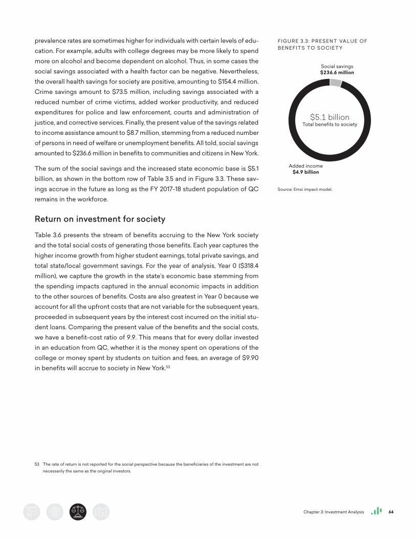
Chapter 3: Investment Analysis 64
prevalence rates are sometimes higher for individuals with certain levels of edu-cation. For example, adults with college degrees may be more likely to spend more on alcohol and become dependent on alcohol. Thus, in some cases the social savings associated with a health factor can be negative. Nevertheless, the overall health savings for society are positive, amounting to $154.4 million. Crime savings amount to $73.5 million, including savings associated with a reduced number of crime victims, added worker productivity, and reduced expenditures for police and law enforcement, courts and administration of justice, and corrective services. Finally, the present value of the savings related to income assistance amount to $8.7 million, stemming from a reduced number of persons in need of welfare or unemployment benefits. All told, social savings amounted to $236.6 million in benefits to communities and citizens in New York.
The sum of the social savings and the increased state economic base is $5.1 billion, as shown in the bottom row of Table 3.5 and in Figure 3.3. These sav-ings accrue in the future as long as the FY 2017-18 student population of QC remains in the workforce.
Return on investment for society
Table 3.6 presents the stream of benefits accruing to the New York society and the total social costs of generating those benefits. Each year captures the higher income growth from higher student earnings, total private savings, and total state/local government savings. For the year of analysis, Year 0 ($318.4 million), we capture the growth in the state’s economic base stemming from the spending impacts captured in the annual economic impacts in addition to the other sources of benefits. Costs are also greatest in Year 0 because we account for all the upfront costs that are not variable for the subsequent years, proceeded in subsequent years by the interest cost incurred on the initial stu-dent loans. Comparing the present value of the benefits and the social costs, we have a benefit-cost ratio of 9.9. This means that for every dollar invested in an education from QC, whether it is the money spent on operations of the college or money spent by students on tuition and fees, an average of $9.90 in benefits will accrue to society in New York.53
53 The rate of return is not reported for the social perspective because the beneficiaries of the investment are not necessarily the same as the original investors.
F I G U R E 3.3 : P R E S E N T VA L U E O F B E N E F I T S TO S O C I E T Y
Source: Emsi impact model.
55+9595+RAdded income
$4.9 billion
Social savings$236.6 million
$5.1 billionTotal benefits to society
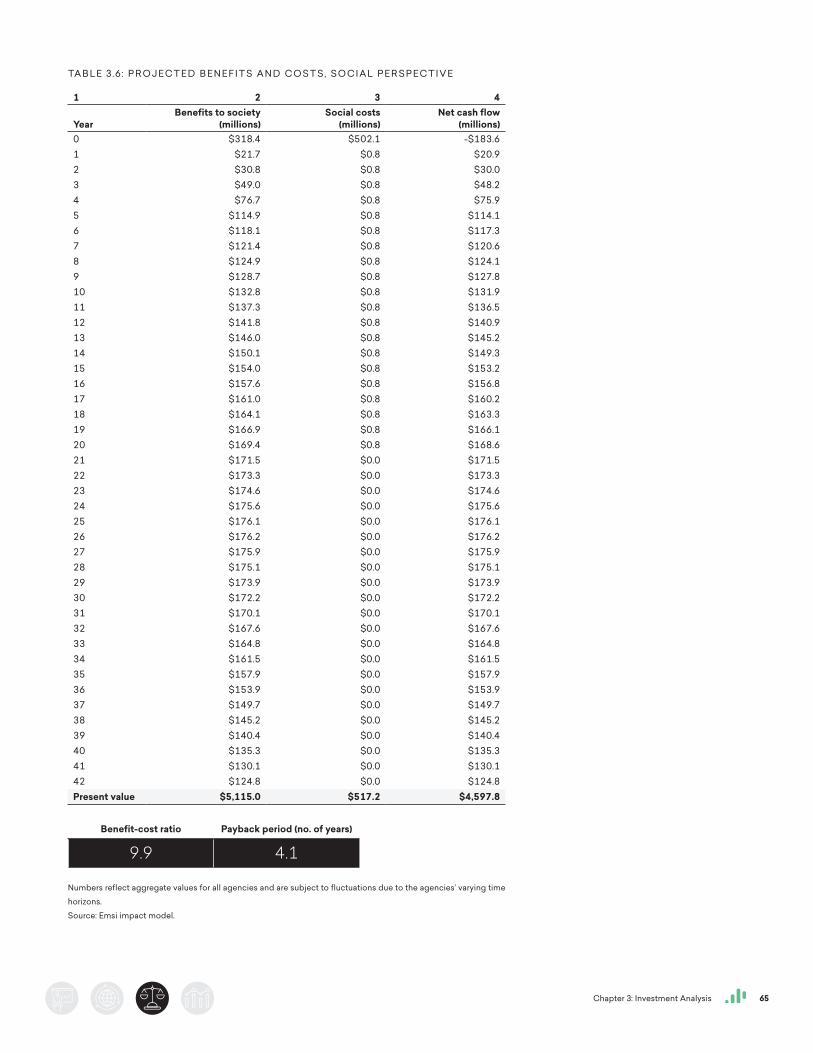
Chapter 3: Investment Analysis 65
TA B L E 3.6: P R O J E C T E D B E N E F I T S A N D C O S T S, S O C I A L P E R S P E C T I V E
1 2 3 4
YearBenefits to society
(millions)Social costs
(millions)Net cash flow
(millions)0 $318.4 $502.1 -$183.61 $21.7 $0.8 $20.92 $30.8 $0.8 $30.03 $49.0 $0.8 $48.24 $76.7 $0.8 $75.95 $114.9 $0.8 $114.16 $118.1 $0.8 $117.37 $121.4 $0.8 $120.68 $124.9 $0.8 $124.19 $128.7 $0.8 $127.810 $132.8 $0.8 $131.911 $137.3 $0.8 $136.512 $141.8 $0.8 $140.913 $146.0 $0.8 $145.214 $150.1 $0.8 $149.315 $154.0 $0.8 $153.216 $157.6 $0.8 $156.817 $161.0 $0.8 $160.218 $164.1 $0.8 $163.319 $166.9 $0.8 $166.120 $169.4 $0.8 $168.621 $171.5 $0.0 $171.522 $173.3 $0.0 $173.323 $174.6 $0.0 $174.624 $175.6 $0.0 $175.625 $176.1 $0.0 $176.126 $176.2 $0.0 $176.227 $175.9 $0.0 $175.928 $175.1 $0.0 $175.129 $173.9 $0.0 $173.930 $172.2 $0.0 $172.231 $170.1 $0.0 $170.132 $167.6 $0.0 $167.633 $164.8 $0.0 $164.834 $161.5 $0.0 $161.535 $157.9 $0.0 $157.936 $153.9 $0.0 $153.937 $149.7 $0.0 $149.738 $145.2 $0.0 $145.239 $140.4 $0.0 $140.440 $135.3 $0.0 $135.341 $130.1 $0.0 $130.142 $124.8 $0.0 $124.8Present value $5,115.0 $517.2 $4,597.8
Benefit-cost ratio Payback period (no. of years)
9.9 4.1
Numbers reflect aggregate values for all agencies and are subject to fluctuations due to the agencies’ varying time
horizons.
Source: Emsi impact model.
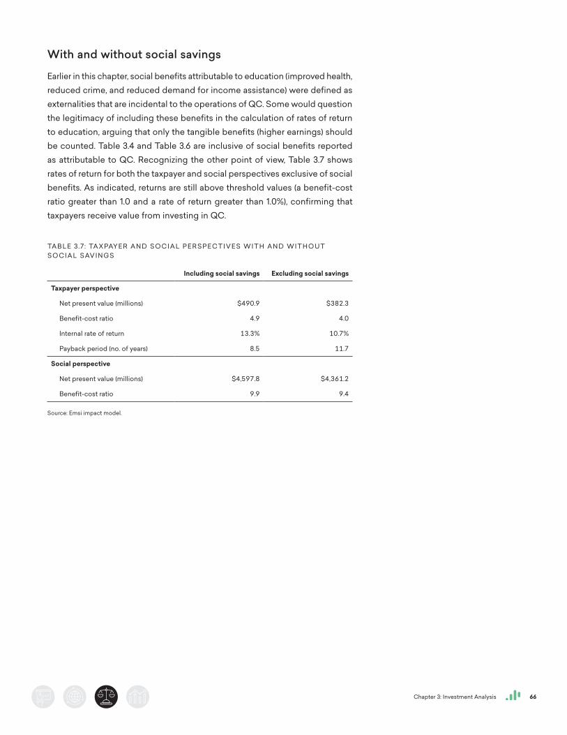
Chapter 3: Investment Analysis 66
With and without social savings
Earlier in this chapter, social benefits attributable to education (improved health, reduced crime, and reduced demand for income assistance) were defined as externalities that are incidental to the operations of QC. Some would question the legitimacy of including these benefits in the calculation of rates of return to education, arguing that only the tangible benefits (higher earnings) should be counted. Table 3.4 and Table 3.6 are inclusive of social benefits reported as attributable to QC. Recognizing the other point of view, Table 3.7 shows rates of return for both the taxpayer and social perspectives exclusive of social benefits. As indicated, returns are still above threshold values (a benefit-cost ratio greater than 1.0 and a rate of return greater than 1.0%), confirming that taxpayers receive value from investing in QC.
TA B L E 3.7 : TA X PAY E R A N D S O C I A L P E R S P E C T I V E S W I T H A N D W I T H O U T S O C I A L SAV I N G S
Including social savings Excluding social savings
Taxpayer perspective
Net present value (millions) $490.9 $382.3
Benefit-cost ratio 4.9 4.0
Internal rate of return 13.3% 10.7%
Payback period (no. of years) 8.5 11.7
Social perspective
Net present value (millions) $4,597.8 $4,361.2
Benefit-cost ratio 9.9 9.4
Source: Emsi impact model.

Chapter 4: Conclusion 67
C H A P T E R 4 :
Conclusion
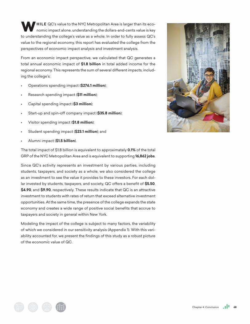
Chapter 4: Conclusion 68
WH I L E QC’s value to the NYC Metropolitan Area is larger than its eco-nomic impact alone, understanding the dollars-and-cents value is key
to understanding the college’s value as a whole. In order to fully assess QC’s value to the regional economy, this report has evaluated the college from the perspectives of economic impact analysis and investment analysis.
From an economic impact perspective, we calculated that QC generates a total annual economic impact of $1.8 billion in total added income for the regional economy. This represents the sum of several different impacts, includ-ing the college’s:
• Operations spending impact ($276.1 million);
• Research spending impact ($11 million);
• Capital spending impact ($3 million);
• Start-up and spin-off company impact ($35.8 million);
• Visitor spending impact ($1.8 million);
• Student spending impact ($23.1 million); and
• Alumni impact ($1.5 billion).
The total impact of $1.8 billion is equivalent to approximately 0.1% of the total GRP of the NYC Metropolitan Area and is equivalent to supporting 16,862 jobs.
Since QC’s activity represents an investment by various parties, including students, taxpayers, and society as a whole, we also considered the college as an investment to see the value it provides to these investors. For each dol-lar invested by students, taxpayers, and society, QC offers a benefit of $5.50, $4.90, and $9.90, respectively. These results indicate that QC is an attractive investment to students with rates of return that exceed alternative investment opportunities. At the same time, the presence of the college expands the state economy and creates a wide range of positive social benefits that accrue to taxpayers and society in general within New York.
Modeling the impact of the college is subject to many factors, the variability of which we considered in our sensitivity analysis (Appendix 1). With this vari-ability accounted for, we present the findings of this study as a robust picture of the economic value of QC.
69Resources and References
Resources and References
Administration for Children and Families. “Fiscal Year 2016 TANF Financial Data.” Office of Family Assistance, TANF Financial Data. 2018. https://www.acf.hhs.gov/ofa/resource/tanf-financial-data-fy-2016.
Arias, Elizabeth. “United States Life Tables, 2008.” National Vital Statistics Reports 61, no. 3 (September 24, 2012). Hyattsville, MD: National Center for Health Statistics. http://www.cdc.gov/nchs/data/nvsr/nvsr61/nvsr61_03.pdf.
Baryla, Edward and Douglas Dotterweich. “Student Migration: Do Significant Factors Vary by Region?” Education Economics 9, no. 3 (2001).
Becker, Gary S. Human Capital: A Theoretical and Empirical Analysis, with Special Reference to Education. New York: Columbia College Press for NBER, 1964.
Bilkic, Natasa, Thomas Gries, and Margarethe Pilichowski. “Stay in School or Start Working? The Human Capital Investment Decision under Uncertainty and Irreversibility.” Labour Economics 19, no. 5 (October 2012): 706-717.
Bureau of Economic Analysis. “Table 1.1.6. Real Gross Domestic Product, Chained Dollars.” GDP and Personal Income. Last modified January 27, 2017. http://www.bea.gov/iTable/iTableHtml.cfm?reqid=9&step=3&isuri=1&903=6.
Bureau of Justice Statistics. “Table 2: Prisoners under the Jurisdiction of State or Federal Correctional Authorities, by Jurisdiction, December 31, 2015 and 2016. Prisoners in 2016, NCJ 251149, 2018. https://www.bjs.gov/content/pub/pdf/p16.pdf.
Bureau of Labor Statistics. “Charts by Topic: Leisure and Sports Activities.” American Time Use Survey. December 2016. http://www.bls.gov/tus/charts/leisure.htm.
Bureau of Labor Statistics. “Charts by Topic: Students.” American Time Use Survey. December 2016. https://www.bls.gov/tus/charts/students.htm.
Bureau of Labor Statistics. “Table 7. Employment status of the civilian nonin-stitutional population 25 years and over by educational attainment, sex, race, and Hispanic or Latino ethnicity.” Current Population Survey, Labor Force Statistics, Household Data Annual Averages, 2017. http://www.bls.gov/cps/cpsaat07.pdf.
Bureau of Labor Statistics. “Table 24: Historical Consumer Price Index for all Urban Consumers (CPI-U): U.S. City Average, All Items.” 2019. https://www.bls.gov/cpi/tables/supplemental-files/historical-cpi-u-201901.pdf.
Emsi is a leading provider of economic impact stud-ies and labor market data to educational institutions, workforce planners, and regional developers in the U.S. and internation-ally. Since 2000, Emsi has completed over 2,000 economic impact studies for educational institutions in three countries. Visit www.economicmodeling.com for more information about Emsi’s products and services.
70Resources and References
Buss, Christian, Jeffrey Parker, and Jon Rivenburg. “Cost, Quality and Enroll-ment Demand at Liberal Arts Colleges.” Economics of Education Review 23, no. 1 (February 2004): 57-65.
Card, David. “The Causal Effect of Education on Earnings.” Handbook of Labor Economics 3 (1999): 1801-1863.
Card, David. “Estimating the Return to Schooling: Progress on Some Persistent Econometric Problems.” Econometrica 69, no. 5 (September 2001): 1127-1160.
Center on Budget and Policy Priorities. “Policy Basics - How Many Weeks of Unemployment are Available?” April 2018. https://www.cbpp.org/sites/default/files/atoms/files/policybasics-uiweeks.pdf.
Centers for Disease Control and Prevention. “Current Cigarette Use Among Adults (Behavior Risk Factor Surveillance System) 2016.” Behavioral Risk Factor Surveillance System Prevalence and Trends Data [Data set]. https://www.cdc.gov/statesystem/cigaretteuseadult.html.
Centers for Disease Control and Prevention. “Heavy Drinkers (Adult Men Hav-ing More Than Two Drinks per Day and Adult Women Having More Than One Drink per Day).” Alcohol Consumption - 2016 Behavioral Risk Factor Surveillance System Prevalence and Trends Data. https://nccd.cdc.gov/BRFSSPrevalence/rdPage.aspx?rdReport=DPH_BRFSS.ExploreByTopic&irbLocationType=StatesAndMMSA&islClass=CLASS01&islTopic=TOPIC30&islYear=2016&islLocation=.
Centers for Disease Control and Prevention. “Table. Characteristics of Current Adult Cigarette Smokers.” National Health Interview Survey, United States, 2016. https://www.cdc.gov/mmwr/volumes/67/wr/mm6702a1.htm#T1_down.
Centers for Medicare and Medicaid Services. “Table 16: National Health Expenditures, Amounts and Average Annual Growth from Previous Year Shown, by Type of Sponsor, Selected Calendar Years 2011-2027.” NHE Projections 2018-2027 – Tables. February 2019. https://www.cms.gov/Research-Statistics-Data-and-Systems/Statistics-Trends-and-Reports/NationalHealthExpendData/NationalHealthAccountsProjected.html.
College Board. “Figure 1: Average Estimated Full-Time Undergraduate Bud-gets, 2018-19 (Enrollment-Weighted).” The College Board, Annual Survey of Colleges, Average Estimated Undergraduate Budgets, 2018-19. https://trends.collegeboard.org/college-pricing/figures-tables/average-estimated-undergraduate-budgets-2018-19.
Congressional Budget Office. “Table 4. Projection of Borrower Interest Rates: CBO’s April 2018 Baseline.” Congressional Budget Office Publications CBO’s April 2018 Baseline Projections for the Student Loan Program. Last modified April 2018. https://www.cbo.gov/system/files?file=2018-06/51310-2018-04-studentloan.pdf.
71Resources and References
Criminal Justice Expenditure and Employment Extracts Program. “Table 4. Justice System Expenditure by Character, State and Type of Government, Fiscal Year 2015” Justice Expenditure and Employment Extracts 2015 (pre-liminary) NCJ 251780. https://www.bjs.gov/index.cfm?ty=dcdetail&iid=286.
Dickerson, Andy, and Steven McIntosh. “The Impact of Distance to Nearest Education Institution on the Post Compulsory Education Participation Decision.” Urban Studies 50, no. 4 (2013): 742-758.
Dynarski, Susan M. “Does Aid Matter? Measuring the Effect of Student Aid on College Attendance and Completion.” American Economic Review 93, no. 1 (2003): 279-288.
Emsi Labor Market Data and Software. www.economicmodeling.com.
Federal Bureau of Investigation, Criminal Justice Information Services Divi-sion. “Table 1: Crime in the United States.” Crime in the United States 2016, Offenses Known to Law Enforcement. https://ucr.fbi.gov/crime-in-the-u.s/2016/crime-in-the-u.s.-2016/tables/table-1.
Federal Bureau of Investigation, Criminal Justice Information Services Division. “Table 18: Estimated Number of Arrests, United States, 2016” in “Uniform Crime Reports.” Crime in the United States, 2016, Persons Arrested. https://ucr.fbi.gov/crime-in-the-u.s/2016/crime-in-the-u.s.-2016/tables/table-18.
Finkelstein, Eric A., Marco da Costa DiBonaventura, Somali M. Burgess, and Brent C. Hale. “The Costs of Obesity in the Workplace.” Journal of Occupational and Environmental Medicine 52, no. 10 (October 2010): 971-976.
Greenberg, Paul, Andree-Anne Fournier, Tammy Sisitsky, Crystal Pike, and Ronald Kesslaer. “The Economic Burden of Adults with Major Depressive Disorder in the United States (2005 and 2010)” Journal of Clinical Psychiatry 76:2, 2015.
Guerino, Paul, Paige M. Harrison, and William J. Sabol. “Prisoners in 2016.” Bureau of Justice Statistics NCJ 236096, January 2018. https://www.bjs.gov/content/pub/pdf/p16.pdf.
Hamadeh, Mohamad and Roy Khoueiri. “Demand Elasticities for Higher Educa-tion in the United States.” International Journal of Business and Economic Perspectives 5, no. 2 (2010): 60-67.
Henderson, James M. and Richard E. Quandt. Microeconomic Theory: A Math-ematical Approach. New York: McGraw-Hill Book Company, 1971.
Hernández-Murillo, Rubén, Lesli S. Ott, Michael T. Owyang, and Denise Wha-len. “Patterns of Interstate Migration in the United States from the Sur-vey of Income and Program Participation.” Federal Reserve Bank of St. Louis Review 93, no. 3 (May/June 2011): 169-186. https://files.stlouisfed.org/files/htdocs/publications/review/11/05/169-186Hernandez.pdf.
72Resources and References
Jaeger, David A. and Marianne E. Page. “New Evidence on Sheepskin Effects in the Returns to Education.” The Review of Economics and Statistics 78, no. 4 (November 1996): 733-740.
Jamal Ahmed, Elyse Phillips, Andrea S. Gentzke, David M. Homa, Stephen D. Babb, Brian A. King, and Linda J. Neff. “Current Cigarette Smoking Among Adults – United States, 2016.” Morbidity and Mortality Weekly Report 2018 67:53-59. DOI: http://dx.doi.org/10.15585/mmwr.mm6702a1.
Kaeding, Nicole. “State Individual Income Tax Rates and Brackets for 2018.” Tax Foundation Fiscal Fact no. 500 (February 2019). https://taxfoundation.org/state-individual-income-tax-rates-brackets-2018.
Kelchtermans, Stijn and Frank Verboven. “Participation and Study Decisions in a Public System of Higher Education.” Journal of Applied Econometrics 25, no. 3 (2010): 355-391.
Leigh, Andrew and Chris Ryan. “Estimating Returns to Education Using Differ-ent Natural Experiments Techniques.” Economics of Education Review 27 (2008): 149-160.
Leonesio, Michael V. “The Economics of Retirement: A Nontechnical Guide.” Social Security Bulletin 59, no. 4 (Winter 1996): 29-50.
McCollister, Kathryn E., Michael T. French, and Hai Fang. “The Cost of Crime to Society: New Crime-Specific Estimates for Policy and Program Evaluation.” Drug and Alcohol Dependence 108, no. 1-2 (April 2010): 98-109. http://www.ncbi.nlm.nih.gov/pmc/articles/PMC2835847.
Mincer, Jacob. “Investment in Human Capital and Personal Income Distribution.” Journal of Political Economy 66, no. 4 (August 1958): 281–302.
Mincer, Jacob. Schooling, Experience and Earnings. New York: National Bureau of Economic Research, 1974.
Morgan, James N. and Edward H. Robb. “The Impact of Age Upon Interregional Migration.” The Annals of Regional Science 15, no. 3 (November 1981): 31-45.
National Center for Education Statistics. Integrated Post-secondary Education Data System (IPEDS). http://nces.ed.gov/ipeds.
National Center for Education Statistics. “Table 219.60 Number of People Taking the GED Test and Percentage Distribution of Those who Passed, by Age Group: 1971 through 2013.” Digest of Education Statistics. 2015. https://nces.ed.gov/programs/digest/d15/tables/dt15_219.60.asp?current=yes.
National Center for Education Statistics. “Table 507.20 Participants in State-Admin-istered Adult Basic Education, Secondary Education, and English as a Second Language Programs, by Type of Program and State or Jurisdiction: Selected Fiscal Years, 2000 through 2014.” Digest of Education Statistics. 2015. https://nces.ed.gov/programs/digest/d15/tables/dt15_507.20.asp?current=yes.
73Resources and References
National Center for Health Statistics. “Table 58. Normal Weight, Overweight, and Obesity Among Persons 20 Years of Age and Over, by Selected Char-acteristics: United States, Selected Years 1988-1994 through 2011-2014.” Centers for Disease Control and Prevention, Health, United States, 2015. https://www.cdc.gov/nchs/data/hus/2015/058.pdf.
National Employment Law Project. “Unemployment Insurance: An Over-view of the Challenges and Strengths of Today’s System”. 2016. https://waysandmeans.house.gov/wp-content/uploads/2016/09/20160907HR-Testimony-Conti.pdf.
National Survey on Drug Use and Health. “Table 19. Illicit Drug Use Disorder in the Past Year, by Age Group and State: Percentages, Annual Averages Based on 2015 and 2016 NSDUHs.” National Survey on Drug Use and Health: Model-Based Prevalence Estimates (50 States and the District of Columbia). https://www.samhsa.gov/data/sites/default/files/NSDUHsaePercents2016/NSDUHsaePercents2016.pdf.
National Survey on Drug Use and Health. “Table 8.59B: Had at Least One Major Depressive Episode (MDE) or MDE with Severe Impairment in Past Year among Persons Aged 18 or Older, and Receipt of Treatment for Depres-sion in Past Year among Persons Aged 18 or Older with MDE or MDE with Severe Impairment in Past Year, by Geographic, Socioeconomic, and Health Characteristics: Percentages, 2015 and 2016.” https://www.samhsa.gov/data/sites/default/files/NSDUH-DetTabs-2016/NSDUH-DetTabs-2016.pdf.
National Survey on Drug Use and Health. “Table 15: Major Depressive Episode in the Past Year, by age group and state: Percentages, annual averages, and P values from tests of differences between percentages, 2008-2009 and 2015-2016.” https://www.samhsa.gov/data/sites/default/files/NSDUHsaeShortTermCHG2016/NSDUHsaeShortTermCHG2016.htm.
Nowotny, Kathryn, Ryan Masters, and Jason Boardman, 2016. “The relationship between education and health among incarcerated man and women in the United States” BMC Public Health. September 2016. https://www.ncbi.nlm.nih.gov/pmc/articles/PMC5009667/.
OECD. “Household Net Saving Rates: As a Percentage of Household Disposable Income.” OECD Factbook 2015-2016: Economic, Environmental and Social Statistics (2016). http://dx.doi.org/10.1787/factbook-2015-19-en.
Office of Management and Budget. “Discount Rates for Cost-Effectiveness Anal-ysis of Federal Programs.” Real Interest Rates on Treasury Notes and Bonds of Specified Maturities (in Percent). Last modified November 2018. https://www.whitehouse.gov/wp-content/uploads/2018/12/Discount-History.pdf.
74Resources and References
Ogden, Cynthia L., Molly M. Lamb, Margaret D. Carroll, and Katherine M. Flegal. “Figure 3. Prevalence of Obesity among Adults Aged 20 Years and Over, by Education, Sex, and Race and Ethnicity: United States 2005-2008.” Obesity and Socioeconomic Status in Adults: United States 2005-2008, National Center for Health Statistics no. 50. (2010).
Ogden Cynthia L., Tala H. Fakhouri, Margaret D. Carroll, Craig M. Hales, Cheryl D. Fryar, Xianfen Li, David S. Freedman. “Prevalence of Obesity Among Adults, by Household Income and Education — United States, 2011–2014” National Center for Health Statistics, Morbidity and Mortality Weekly Report, 66:1369–1373 (2017). https://www.cdc.gov/mmwr/volumes/66/wr/mm6650a1.htm?s_cid=mm6650a1_w#suggestedcitation.
Polachek, Solomon W. “Earnings Over the Lifecycle: The Mincer Earnings Func-tion and its Applications.” Foundations and Trends in Microeconomics 4, no. 3 (2008): 165-272.
Polachek, Solomon W. “Mincer’s Overtaking Point and the Lifecycle Earnings Distribution.” Review of the Economics of the Household 1, no. 4 (December 2003): 273-304.
Ramey, Valerie and Neville Francis. “A Century of Work and Leisure.” American Economic Journal: Macroeconomics 1, no. 2 (2009): 189-224.
Sacks, Gonzales, Bouchery, Tomedi, & Brewer (2015). 2010 National and State Costs of Excessive Alcohol Consumption. American Journal of Preven-tive Medicine, 49(5), E73-E79. https://www.ajpmonline.org/article/S0749-3797(15)00354-2/pdf/.
Sevilla, Almudena, Jose Ignacio Gimenez-Nadal, and Jonathan I. Gershuny. “Leisure Inequality in the United States: 1965-2003.” IZA Discussion Paper no. 6708 (July 2012).
Social Security Administration. “Retirement Benefits.” Full Retirement Age. May 2016. https://www.ssa.gov/pubs/EN-05-10035.pdf.
State of Obesity. “Adult Obesity in the United States.” Adult Obesity Rate by State, 2016. https://stateofobesity.org/adult-obesity/.
Substance Abuse and Mental Health Services Administration. “Table A.2. Spending by Payer: Levels and Percent Distribution for Mental Health and Substance Abuse (MHSA), Mental Health (MH), Substance Abuse (SA), Alco-hol Abuse (AA), Drug Abuse (DA), and All-Health, 2014.” Behavioral Health Spending & Use Accounts, 1986 – 2014. HHS Publication No. SMA-16-4975, 2016. https://store.samhsa.gov/shin/content/SMA16-4975/SMA16-4975.pdf.
75Resources and References
Substance Abuse and Mental Health Services Administration. “Table 5.4B - Illicit Drug Use Disorder in Past Year among Persons Aged 12 or Older, by Age Group and Demographic Characteristics: Percentages, 2015 and 2016” SAM-SHA, Center for Behaviorial Health Statistics and Quality, National Survey on Drug Use and Health, 2015 and 2016. https://www.samhsa.gov/data/sites/default/files/NSDUH-DetTabs-2016/NSDUH-DetTabs-2016.htm#tab5-4B.
Substance Abuse and Mental Health Services Administration. “Table 5.5B - Alcohol Use Disorder in the Past Year among Persons Aged 18 or Older, by Demographic Characteristics: Percentages, 2015 and 2016.” SAMSHA, Center for Behavioral Health Statistics and Quality, National Survey on Drug Use and Health, 2015 and 2016. https://www.samhsa.gov/data/sites/default/files/NSDUH-DetTabs-2016/NSDUH-DetTabs-2016.htm#tab5-6A.
Supplemental Nutrition Assistance Program. “State Activity Report Fiscal Year 2016.” Food and Nutrition Service, Supplemental Nutrition Assistance Program, Program Accountability and Administration Division (September 2017). https://fns-prod.azureedge.net/sites/default/files/snap/FY16-State-Activity-Report.pdf.
U.S. Census Bureau. “Annual Estimates of the Resident Population for Selected Age Groups by Sex: April 1, 2010 to July 1, 2015.” National Population by Characteristics Tables: 2010-2015. December 2016. http://www.census.gov/data/tables/2015/demo/popest/nation-detail.html.
U.S. Census Bureau. “Educational Characteristics of Prisoners: Data from the ACS.” 2011. https://www.census.gov/library/working-papers/2011/demo/SEHSD-WP2011-08.html.
U.S. Census Bureau. “Social Insurance and Human Services.” The 2012 Statistical Abstract. http://www.census.gov/compendia/statab/cats/social_insurance_human_services.html.
U.S. Department of Agriculture, Office of Policy Support. Supplemental Nutri-tion Assistance Program Nutrition Assistance Program Report Series. “Characteristics of Supplemental Nutrition Assistance Program Households: Fiscal Year 2016.” https://fns-prod.azureedge.net/sites/default/files/ops/Characteristics2016.pdf.
U.S. Department of Education, Federal Student Aid Office. “The Standard Repayment Plan.” https://studentaid.ed.gov/sa/repay-loans/understand/plans/standard.
U.S. Department of Health and Human Services. “2016 Welfare Indicators and Risk Factors: Fifteenth Report to Congress” Annual Report to Congress, 2016. https://aspe.hhs.gov/system/files/pdf/206736/WelfareIndicators15thReport.pdf.
76Resources and References
U.S. Department of Health and Human Services, Office of Family Assistance. “Characteristics and Financial Circumstances of TANF Recipients, Fis-cal Year 2016.” https://www.acf.hhs.gov/ofa/resource/characteristics-and-financial-circumstances-of-tanf-recipients-fiscal-year-2016-0.
U.S. Department of Health & Human Services. “The Health Consequences of Smoking—50 Years of Progress.” A Report of the Surgeon General, 2014. https://www.surgeongeneral.gov/library/reports/50-years-of-progress/50-years-of-progress-by-section.html.
U.S. Department of Labor. “Unemployment Insurance Data Summary, 4th Quarter 2017.” https://workforcesecurity.doleta.gov/unemploy/content/data_stats/datasum17/DataSum_2017_4.pdf.
Walczak, Jared, Scott Drenkard. “State and Local Sales Tax Rates, Midyear 2018.” Tax Foundation Fiscal Fact no. 600 (July 2018). https://files.taxfoundation.org/20180713135343/Tax-Foundation-FF600.pdf.
Walden, Michael, “The Local Economic Impact of the Cooperating Raleigh Colleges: Update 2013.” March 2014. http://crcraleighcolleges.org/files/crcimpact2013-final.pdf.
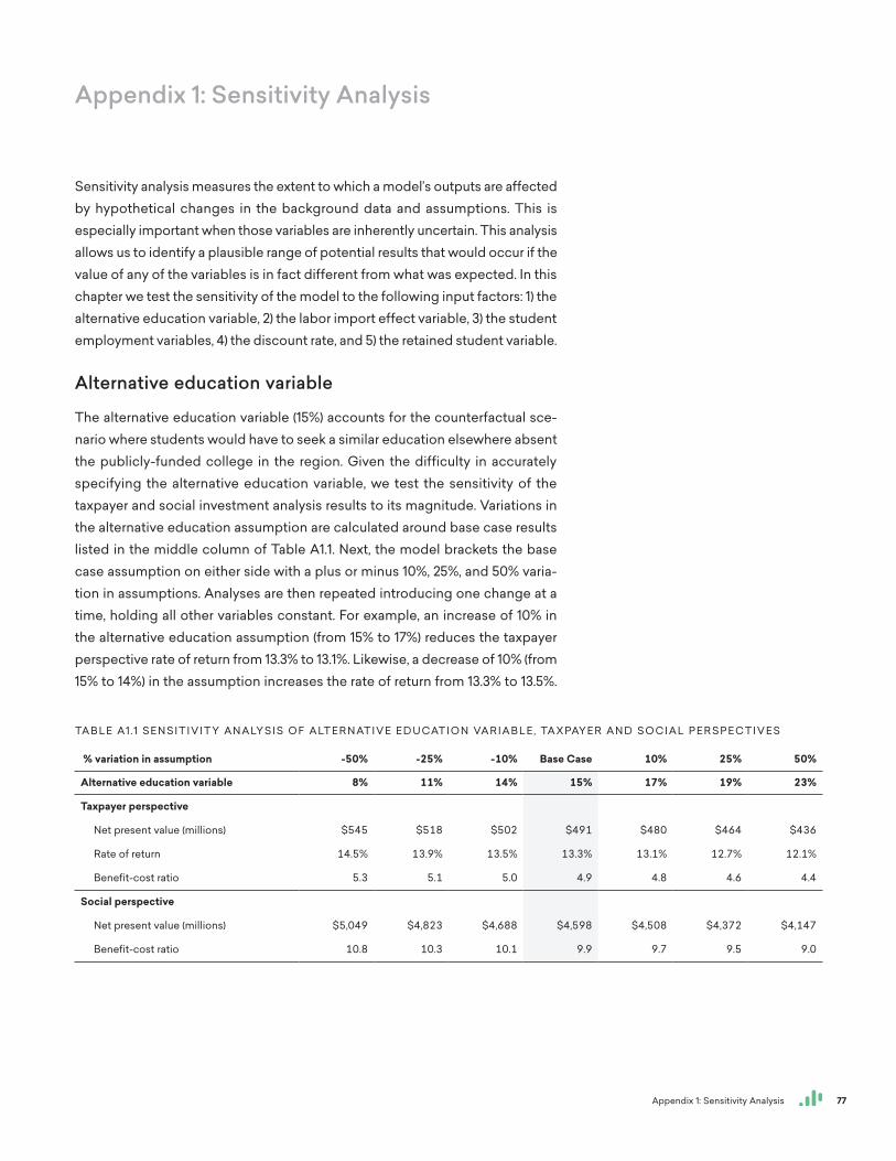
77Appendix 1: Sensitivity Analysis
Appendix 1: Sensitivity Analysis
Sensitivity analysis measures the extent to which a model’s outputs are affected by hypothetical changes in the background data and assumptions. This is especially important when those variables are inherently uncertain. This analysis allows us to identify a plausible range of potential results that would occur if the value of any of the variables is in fact different from what was expected. In this chapter we test the sensitivity of the model to the following input factors: 1) the alternative education variable, 2) the labor import effect variable, 3) the student employment variables, 4) the discount rate, and 5) the retained student variable.
Alternative education variable
The alternative education variable (15%) accounts for the counterfactual sce-nario where students would have to seek a similar education elsewhere absent the publicly-funded college in the region. Given the difficulty in accurately specifying the alternative education variable, we test the sensitivity of the taxpayer and social investment analysis results to its magnitude. Variations in the alternative education assumption are calculated around base case results listed in the middle column of Table A1.1. Next, the model brackets the base case assumption on either side with a plus or minus 10%, 25%, and 50% varia-tion in assumptions. Analyses are then repeated introducing one change at a time, holding all other variables constant. For example, an increase of 10% in the alternative education assumption (from 15% to 17%) reduces the taxpayer perspective rate of return from 13.3% to 13.1%. Likewise, a decrease of 10% (from 15% to 14%) in the assumption increases the rate of return from 13.3% to 13.5%.
TA B L E A1.1 S E N S I T I V I T Y A N A LY S I S O F A LT E R N AT I V E E D U CAT I O N VA R I A B L E, TA X PAY E R A N D S O C I A L P E R S P E C T I V E S
% variation in assumption -50% -25% -10% Base Case 10% 25% 50%
Alternative education variable 8% 11% 14% 15% 17% 19% 23%
Taxpayer perspective
Net present value (millions) $545 $518 $502 $491 $480 $464 $436
Rate of return 14.5% 13.9% 13.5% 13.3% 13.1% 12.7% 12.1%
Benefit-cost ratio 5.3 5.1 5.0 4.9 4.8 4.6 4.4
Social perspective
Net present value (millions) $5,049 $4,823 $4,688 $4,598 $4,508 $4,372 $4,147
Benefit-cost ratio 10.8 10.3 10.1 9.9 9.7 9.5 9.0
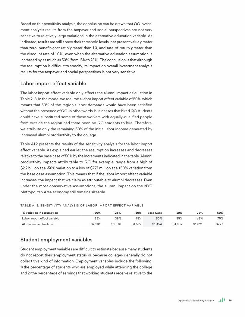
78Appendix 1: Sensitivity Analysis
Based on this sensitivity analysis, the conclusion can be drawn that QC invest-ment analysis results from the taxpayer and social perspectives are not very sensitive to relatively large variations in the alternative education variable. As indicated, results are still above their threshold levels (net present value greater than zero, benefit-cost ratio greater than 1.0, and rate of return greater than the discount rate of 1.0%), even when the alternative education assumption is increased by as much as 50% (from 15% to 23%). The conclusion is that although the assumption is difficult to specify, its impact on overall investment analysis results for the taxpayer and social perspectives is not very sensitive.
Labor import effect variable
The labor import effect variable only affects the alumni impact calculation in Table 2.13. In the model we assume a labor import effect variable of 50%, which means that 50% of the region’s labor demands would have been satisfied without the presence of QC. In other words, businesses that hired QC students could have substituted some of these workers with equally-qualified people from outside the region had there been no QC students to hire. Therefore, we attribute only the remaining 50% of the initial labor income generated by increased alumni productivity to the college.
Table A1.2 presents the results of the sensitivity analysis for the labor import effect variable. As explained earlier, the assumption increases and decreases relative to the base case of 50% by the increments indicated in the table. Alumni productivity impacts attributable to QC, for example, range from a high of $2.2 billion at a -50% variation to a low of $727 million at a +50% variation from the base case assumption. This means that if the labor import effect variable increases, the impact that we claim as attributable to alumni decreases. Even under the most conservative assumptions, the alumni impact on the NYC Metropolitan Area economy still remains sizeable.
Student employment variables
Student employment variables are difficult to estimate because many students do not report their employment status or because colleges generally do not collect this kind of information. Employment variables include the following: 1) the percentage of students who are employed while attending the college and 2) the percentage of earnings that working students receive relative to the
TA B L E A1.2 : S E N S I T I V I T Y A N A LY S I S O F L A B O R I M P O RT E F F E C T VA R I A B L E
% variation in assumption -50% -25% -10% Base Case 10% 25% 50%
Labor import effect variable 25% 38% 45% 50% 55% 63% 75%
Alumni impact (millions) $2,181 $1,818 $1,599 $1,454 $1,309 $1,091 $727
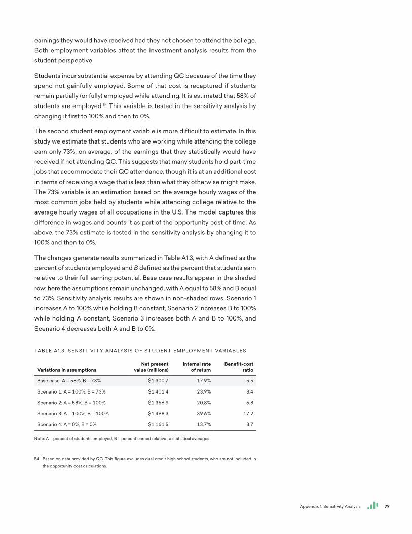
79Appendix 1: Sensitivity Analysis
earnings they would have received had they not chosen to attend the college. Both employment variables affect the investment analysis results from the student perspective.
Students incur substantial expense by attending QC because of the time they spend not gainfully employed. Some of that cost is recaptured if students remain partially (or fully) employed while attending. It is estimated that 58% of students are employed.54 This variable is tested in the sensitivity analysis by changing it first to 100% and then to 0%.
The second student employment variable is more difficult to estimate. In this study we estimate that students who are working while attending the college earn only 73%, on average, of the earnings that they statistically would have received if not attending QC. This suggests that many students hold part-time jobs that accommodate their QC attendance, though it is at an additional cost in terms of receiving a wage that is less than what they otherwise might make. The 73% variable is an estimation based on the average hourly wages of the most common jobs held by students while attending college relative to the average hourly wages of all occupations in the U.S. The model captures this difference in wages and counts it as part of the opportunity cost of time. As above, the 73% estimate is tested in the sensitivity analysis by changing it to 100% and then to 0%.
The changes generate results summarized in Table A1.3, with A defined as the percent of students employed and B defined as the percent that students earn relative to their full earning potential. Base case results appear in the shaded row; here the assumptions remain unchanged, with A equal to 58% and B equal to 73%. Sensitivity analysis results are shown in non-shaded rows. Scenario 1 increases A to 100% while holding B constant, Scenario 2 increases B to 100% while holding A constant, Scenario 3 increases both A and B to 100%, and Scenario 4 decreases both A and B to 0%.
54 Based on data provided by QC. This figure excludes dual credit high school students, who are not included in the opportunity cost calculations.
TA B L E A1.3 : S E N S I T I V I T Y A N A LY S I S O F S T U D E N T E M P LOY M E N T VA R I A B L E S
Variations in assumptionsNet present
value (millions)Internal rate
of returnBenefit-cost
ratio
Base case: A = 58%, B = 73% $1,300.7 17.9% 5.5
Scenario 1: A = 100%, B = 73% $1,401.4 23.9% 8.4
Scenario 2: A = 58%, B = 100% $1,356.9 20.8% 6.8
Scenario 3: A = 100%, B = 100% $1,498.3 39.6% 17.2
Scenario 4: A = 0%, B = 0% $1,161.5 13.7% 3.7
Note: A = percent of students employed; B = percent earned relative to statistical averages
80Appendix 1: Sensitivity Analysis
• Scenario 1: Increasing the percentage of students employed (A) from 58% to 100%, the net present value, internal rate of return, and benefit-cost ratio improve to $1.4 billion, 23.9%, and 8.4, respectively, relative to base case results. Improved results are attributable to a lower opportunity cost of time; all students are employed in this case.
• Scenario 2: Increasing earnings relative to statistical averages (B) from 73% to 100%, the net present value, internal rate of return, and benefit-cost ratio results improve to $1.4 billion, 20.8%, and 6.8, respectively, relative to base case results; a strong improvement, again attributable to a lower opportunity cost of time.
• Scenario 3: Increasing both assumptions A and B to 100% simultaneously, the net present value, internal rate of return, and benefit-cost ratio improve yet further to $1.5 billion, 39.6%, and 17.2, respectively, relative to base case results. This scenario assumes that all students are fully employed and earning full salaries (equal to statistical averages) while attending classes.
• Scenario 4: Finally, decreasing both A and B to 0% reduces the net present value, internal rate of return, and benefit-cost ratio to $1.2 billion, 13.7%, and 3.7, respectively, relative to base case results. These results are reflective of an increased opportunity cost; none of the students are employed in this case.55
It is strongly emphasized in this section that base case results are very attractive in that results are all above their threshold levels. As is clearly demonstrated here, results of the first three alternative scenarios appear much more attractive, although they overstate benefits. Results presented in Chapter 3 are realistic, indicating that investments in QC generate excellent returns, well above the long-term average percent rates of return in stock and bond markets.
Discount rate
The discount rate is a rate of interest that converts future monies to their present value. In investment analysis, the discount rate accounts for two fundamental principles: 1) the time value of money, and 2) the level of risk that an investor is willing to accept. Time value of money refers to the value of money after interest or inflation has accrued over a given length of time. An investor must be willing to forego the use of money in the present to receive compensation for it in the future. The discount rate also addresses the investors’ risk prefer-ences by serving as a proxy for the minimum rate of return that the proposed risky asset must be expected to yield before the investors will be persuaded to invest in it. Typically, this minimum rate of return is determined by the known
55 Note that reducing the percent of students employed to 0% automatically negates the percent they earn relative to full earning potential, since none of the students receive any earnings in this case.
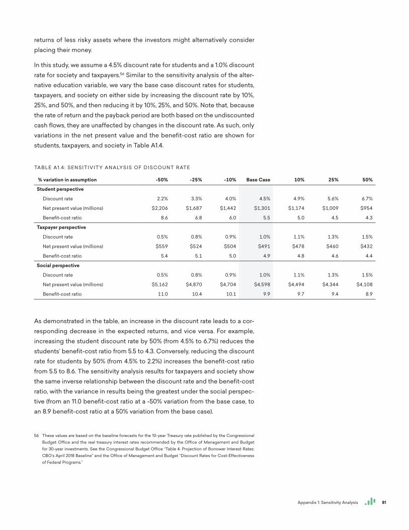
81Appendix 1: Sensitivity Analysis
returns of less risky assets where the investors might alternatively consider placing their money.
In this study, we assume a 4.5% discount rate for students and a 1.0% discount rate for society and taxpayers.56 Similar to the sensitivity analysis of the alter-native education variable, we vary the base case discount rates for students, taxpayers, and society on either side by increasing the discount rate by 10%, 25%, and 50%, and then reducing it by 10%, 25%, and 50%. Note that, because the rate of return and the payback period are both based on the undiscounted cash flows, they are unaffected by changes in the discount rate. As such, only variations in the net present value and the benefit-cost ratio are shown for students, taxpayers, and society in Table A1.4.
As demonstrated in the table, an increase in the discount rate leads to a cor-responding decrease in the expected returns, and vice versa. For example, increasing the student discount rate by 50% (from 4.5% to 6.7%) reduces the students’ benefit-cost ratio from 5.5 to 4.3. Conversely, reducing the discount rate for students by 50% (from 4.5% to 2.2%) increases the benefit-cost ratio from 5.5 to 8.6. The sensitivity analysis results for taxpayers and society show the same inverse relationship between the discount rate and the benefit-cost ratio, with the variance in results being the greatest under the social perspec-tive (from an 11.0 benefit-cost ratio at a -50% variation from the base case, to an 8.9 benefit-cost ratio at a 50% variation from the base case).
56 These values are based on the baseline forecasts for the 10-year Treasury rate published by the Congressional Budget Office and the real treasury interest rates recommended by the Office of Management and Budget for 30-year investments. See the Congressional Budget Office “Table 4. Projection of Borrower Interest Rates: CBO’s April 2018 Baseline” and the Office of Management and Budget “Discount Rates for Cost-Effectiveness of Federal Programs.”
TA B L E A1.4: S E N S I T I V I T Y A N A LY S I S O F D I S C O U N T R AT E
% variation in assumption -50% -25% -10% Base Case 10% 25% 50%
Student perspective
Discount rate 2.2% 3.3% 4.0% 4.5% 4.9% 5.6% 6.7%
Net present value (millions) $2,206 $1,687 $1,442 $1,301 $1,174 $1,009 $954
Benefit-cost ratio 8.6 6.8 6.0 5.5 5.0 4.5 4.3
Taxpayer perspective
Discount rate 0.5% 0.8% 0.9% 1.0% 1.1% 1.3% 1.5%
Net present value (millions) $559 $524 $504 $491 $478 $460 $432
Benefit-cost ratio 5.4 5.1 5.0 4.9 4.8 4.6 4.4
Social perspective
Discount rate 0.5% 0.8% 0.9% 1.0% 1.1% 1.3% 1.5%
Net present value (millions) $5,162 $4,870 $4,704 $4,598 $4,494 $4,344 $4,108
Benefit-cost ratio 11.0 10.4 10.1 9.9 9.7 9.4 8.9
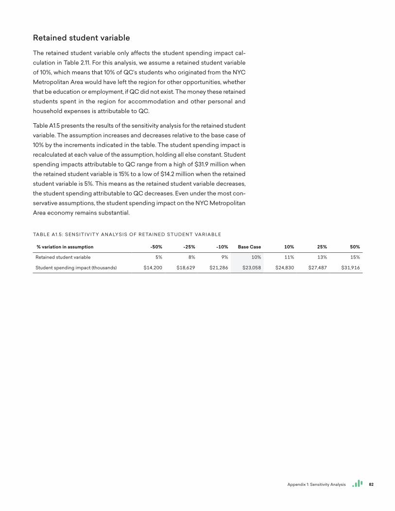
82Appendix 1: Sensitivity Analysis
Retained student variable
The retained student variable only affects the student spending impact cal-culation in Table 2.11. For this analysis, we assume a retained student variable of 10%, which means that 10% of QC’s students who originated from the NYC Metropolitan Area would have left the region for other opportunities, whether that be education or employment, if QC did not exist. The money these retained students spent in the region for accommodation and other personal and household expenses is attributable to QC.
Table A1.5 presents the results of the sensitivity analysis for the retained student variable. The assumption increases and decreases relative to the base case of 10% by the increments indicated in the table. The student spending impact is recalculated at each value of the assumption, holding all else constant. Student spending impacts attributable to QC range from a high of $31.9 million when the retained student variable is 15% to a low of $14.2 million when the retained student variable is 5%. This means as the retained student variable decreases, the student spending attributable to QC decreases. Even under the most con-servative assumptions, the student spending impact on the NYC Metropolitan Area economy remains substantial.
TA B L E A1.5 : S E N S I T I V I T Y A N A LY S I S O F R E TA I N E D S T U D E N T VA R I A B L E
% variation in assumption -50% -25% -10% Base Case 10% 25% 50%
Retained student variable 5% 8% 9% 10% 11% 13% 15%
Student spending impact (thousands) $14,200 $18,629 $21,286 $23,058 $24,830 $27,487 $31,916
83Appendix 2: Glossary of Terms
Appendix 2: Glossary of Terms
Alternative education A “with” and “without” measure of the percent of stu-dents who would still be able to avail themselves of education if the college under analysis did not exist. An estimate of 10%, for example, means that 10% of students do not depend directly on the existence of the college in order to obtain their education.
Alternative use of funds A measure of how monies that are currently used to fund the college might otherwise have been used if the college did not exist.
Asset value Capitalized value of a stream of future returns. Asset value mea-sures what someone would have to pay today for an instrument that pro-vides the same stream of future revenues.
Attrition rate Rate at which students leave the workforce due to out-migration, unemployment, retirement, or death.
Benefit-cost ratio Present value of benefits divided by present value of costs. If the benefit-cost ratio is greater than 1, then benefits exceed costs, and the investment is feasible.
Counterfactual scenario What would have happened if a given event had not occurred. In the case of this economic impact study, the counterfactual scenario is a scenario where the college did not exist.
Credit hour equivalent Credit hour equivalent, or CHE, is defined as 15 contact hours of education if on a semester system, and 10 contact hours if on a quarter system. In general, it requires 450 contact hours to complete one full-time equivalent, or FTE.
Demand Relationship between the market price of education and the volume of education demanded (expressed in terms of enrollment). The law of the downward-sloping demand curve is related to the fact that enrollment increases only if the price (tuition and fees) is lowered, or conversely, enroll-ment decreases if price increases.
Discounting Expressing future revenues and costs in present value terms.
Earnings (labor income) Income that is received as a result of labor; i.e., wages.
Economics Study of the allocation of scarce resources among alternative and competing ends. Economics is not normative (what ought to be done), but positive (describes what is, or how people are likely to behave in response to economic changes).
84Appendix 2: Glossary of Terms
Elasticity of demand Degree of responsiveness of the quantity of education demanded (enrollment) to changes in market prices (tuition and fees). If a decrease in fees increases or decreases total enrollment by a significant amount, demand is elastic. If enrollment remains the same or changes only slightly, demand is inelastic.
Externalities Impacts (positive and negative) for which there is no compensa-tion. Positive externalities of education include improved social behaviors such as improved health, lower crime, and reduced demand for income assistance. Educational institutions do not receive compensation for these benefits, but benefits still occur because education is statistically proven to lead to improved social behaviors.
Gross regional product Measure of the final value of all goods and services produced in a region after netting out the cost of goods used in production. Alternatively, gross regional product (GRP) equals the combined incomes of all factors of production; i.e., labor, land and capital. These include wages, salaries, proprietors’ incomes, profits, rents, and other. Gross regional prod-uct is also sometimes called value added or added income.
Initial effect Income generated by the initial injection of monies into the economy through the payroll of the college and the higher earnings of its students.
Input-output analysis Relationship between a given set of demands for final goods and services and the implied amounts of manufactured inputs, raw materials, and labor that this requires. When educational institutions pay wages and salaries and spend money for supplies in the region, they also generate earnings in all sectors of the economy, thereby increasing the demand for goods and services and jobs. Moreover, as students enter or rejoin the workforce with higher skills, they earn higher salaries and wages. In turn, this generates more consumption and spending in other sectors of the economy.
Internal rate of return Rate of interest that, when used to discount cash flows associated with investing in education, reduces its net present value to zero (i.e., where the present value of revenues accruing from the invest-ment are just equal to the present value of costs incurred). This, in effect, is the breakeven rate of return on investment since it shows the highest rate of interest at which the investment makes neither a profit nor a loss.
Multiplier effect Additional income created in the economy as the college and its students spend money in the region. It consists of the income cre-ated by the supply chain of the industries initially affected by the spending of the college and its students (i.e., the direct effect), income created by the supply chain of the initial supply chain (i.e., the indirect effect), and the income created by the increased spending of the household sector (i.e., the induced effect).
85Appendix 2: Glossary of Terms
NAICS The North American Industry Classification System (NAICS) classifies North American business establishment in order to better collect, analyze, and publish statistical data related to the business economy.
Net cash flow Benefits minus costs, i.e., the sum of revenues accruing from an investment minus costs incurred.
Net present value Net cash flow discounted to the present. All future cash flows are collapsed into one number, which, if positive, indicates feasibility. The result is expressed as a monetary measure.
Non-labor income Income received from investments, such as rent, interest, and dividends.
Opportunity cost Benefits foregone from alternative B once a decision is made to allocate resources to alternative A. Or, if individuals choose to attend college, they forego earnings that they would have received had they chose instead to work full-time. Foregone earnings, therefore, are the “price tag” of choosing to attend college.
Payback period Length of time required to recover an investment. The shorter the period, the more attractive the investment. The formula for computing payback period is:
Payback period = cost of investment/net return per period
86Appendix 3: Frequently Asked Questions (FAQs)
Appendix 3: Frequently Asked Questions (FAQs)
This appendix provides answers to some frequently asked questions about the results.
What is economic impact analysis?
Economic impact analysis quantifies the impact from a given economic event—in this case, the presence of a college—on the economy of a specified region.
What is investment analysis?
Investment analysis is a standard method for determining whether or not an existing or proposed investment is economically viable. This methodology is appropriate in situations where a stakeholder puts up a certain amount of money with the expectation of receiving benefits in return, where the benefits that the stakeholder receives are distributed over time, and where a discount rate must be applied in order to account for the time value of money.
Do the results differ by region, and if so, why?
Yes. Regional economic data are drawn from Emsi’s proprietary MR-SAM model, the Census Bureau, and other sources to reflect the specific earnings levels, jobs numbers, unemployment rates, population demographics, and other key characteristics of the region served by the college. Therefore, model results for the college are specific to the given region.
Are the funds transferred to the college increasing in value, or simply being re-directed?
Emsi’s approach is not a simple “rearranging of the furniture” where the impact of operations spending is essentially a restatement of the level of funding received by the college. Rather, it is an impact assessment of the additional income created in the region as a result of the college spending on payroll and other non-pay expenditures, net of any impacts that would have occurred anyway if the college did not exist.
87Appendix 3: Frequently Asked Questions (FAQs)
How does my college’s rates of return compare to that of other institutions?
In general, Emsi discourages comparisons between institutions since many factors, such as regional economic conditions, institutional differences, and student demographics are outside of the college’s control. It is best to com-pare the rate of return to the discount rates of 4.5% (for students) and 1.0% (for society and taxpayers), which can also be seen as the opportunity cost of the investment (since these stakeholder groups could be spending their time and money in other investment schemes besides education). If the rate of return is higher than the discount rate, the stakeholder groups can expect to receive a positive return on their educational investment.
Emsi recognizes that some institutions may want to make comparisons. As a word of caution, if comparing to an institution that had a study commissioned by a firm other than Emsi, then differences in methodology will create an “apples to oranges” comparison and will therefore be difficult. The study results should be seen as unique to each institution.
Net present value (NPV): How do I communicate this in laymen’s terms?
Which would you rather have: a dollar right now or a dollar 30 years from now? That most people will choose a dollar now is the crux of net present value. The preference for a dollar today means today’s dollar is therefore worth more than it would be in the future (in most people’s opinion). Because the dollar today is worth more than a dollar in 30 years, the dollar 30 years from now needs to be adjusted to express its worth today. Adjusting the values for this “time value of money” is called discounting and the result of adding them all up after discount-ing each value is called net present value.
Internal rate of return (IRR): How do I communicate this in laymen’s terms?
Using the bank as an example, an individual needs to decide between spending all of their paycheck today and putting it into savings. If they spend it today, they know what it is worth: $1 = $1. If they put it into savings, they need to know that there will be some sort of return to them for spending those dollars in the future rather than now. This is why banks offer interest rates and deposit interest earnings. This makes it so an individual can expect, for example, a 3% return in the future for money that they put into savings now.
88Appendix 3: Frequently Asked Questions (FAQs)
Total economic impact: How do I communicate this in laymen’s terms?
Big numbers are great, but putting them into perspective can be a challenge. To add perspective, find an industry with roughly the same “% of GRP” as your college (Table 1.3). This percentage represents its portion of the total gross regional product in the region (similar to the nationally recognized gross domestic product but at a regional level). This allows the college to say that their single brick and mortar campus does just as much for the NYC Metropolitan Area as the entire Utilities industry, for example. This powerful statement can help put the large total impact number into perspective.
89Appendix 4: Example of Sales versus Income
Appendix 4: Example of Sales versus Income
Emsi’s economic impact study differs from many other studies because we prefer to report the impacts in terms of income rather than sales (or output). Income is synonymous with value added or gross regional product (GRP). Sales include all the intermediary costs associated with producing goods and services. Income is a net measure that excludes these intermediary costs:
Income = Sales – Intermediary Costs
For this reason, income is a more meaningful measure of new economic activity than reporting sales. This is evidenced by the use of gross domestic product (GDP)—a measure of income—by economists when considering the economic growth or size of a country. The difference is GRP reflects a region and GDP a country.
To demonstrate the difference between income and sales, let us consider an example of a baker’s production of a loaf of bread. The baker buys the ingre-dients such as eggs, flour, and yeast for $2.00. He uses capital such as a mixer to combine the ingredients and an oven to bake the bread and convert it into a final product. Overhead costs for these steps are $1.00. Total intermediary costs are $3.00. The baker then sells the loaf of bread for $5.00.
The sales amount of the loaf of bread is $5.00. The income from the loaf of bread is equal to the sales amount less the intermediary costs:
Income = $5.00 − $3.00 = $2.00
In our analysis, we provide context behind the income figures by also report-ing the associated number of jobs. The impacts are also reported in sales and earnings terms for reference.
90Appendix 5: Emsi MR-SAM
Appendix 5: Emsi MR-SAM
Emsi’s MR-SAM represents the flow of all economic transactions in a given region. It replaces Emsi’s previous input-output (IO) model, which operated with some 1,000 industries, four layers of government, a single household consumption sector, and an investment sector. The old IO model was used to simulate the ripple effects (i.e., multipliers) in the regional economy as a result of industries entering or exiting the region. The MR-SAM model performs the same tasks as the old IO model, but it also does much more. Along with the same 1,000 industries, government, household and investment sectors embedded in the old IO tool, the MR-SAM exhibits much more functionality, a greater amount of data, and a higher level of detail on the demographic and occupational components of jobs (16 demographic cohorts and about 750 occupations are characterized).
This appendix presents a high-level overview of the MR-SAM. Additional documentation on the technical aspects of the model is available upon request.
Data sources for the model
The Emsi MR-SAM model relies on a number of internal and external data sources, mostly compiled by the federal government. What follows is a listing and short explanation of our sources. The use of these data will be covered in more detail later in this appendix.
Emsi Data are produced from many data sources to produce detailed industry, occupation, and demographic jobs and earnings data at the local level. This information (especially sales-to-jobs ratios derived from jobs and earnings-to-sales ratios) is used to help regionalize the national matrices as well as to disaggregate them into more detailed industries than are normally available.
BEA Make and Use Tables (MUT) are the basis for input-output models in the U.S. The make table is a matrix that describes the amount of each commod-ity made by each industry in a given year. Industries are placed in the rows and commodities in the columns. The use table is a matrix that describes the amount of each commodity used by each industry in a given year. In the use table, commodities are placed in the rows and industries in the columns. The BEA produces two different sets of MUTs, the benchmark and the summary. The benchmark set contains about 500 sectors and is released every five years, with a five-year lag time (e.g., 2002 benchmark MUTs were released in 2007). The summary set contains about 80 sectors and is released every year, with a two-year lag (e.g., 2010 summary MUTs were released in late 2011/early 2012).
91Appendix 5: Emsi MR-SAM
The MUTs are used in the Emsi MR-SAM model to produce an industry-by-industry matrix describing all industry purchases from all industries.
BEA Gross Domestic Product by State (GSP) describes gross domestic product from the value added (also known as added income) perspective. Value added is equal to employee compensation, gross operating surplus, and taxes on pro-duction and imports, less subsidies. Each of these components is reported for each state and an aggregate group of industries. This dataset is updated once per year, with a one-year lag. The Emsi MR-SAM model makes use of this data as a control and pegs certain pieces of the model to values from this dataset.
BEA National Income and Product Accounts (NIPA) cover a wide variety of economic measures for the nation, including gross domestic product (GDP), sources of output, and distribution of income. This dataset is updated periodi-cally throughout the year and can be between a month and several years old depending on the specific account. NIPA data are used in many of the Emsi MR-SAM processes as both controls and seeds.
BEA Local Area Income (LPI) encapsulates multiple tables with geographies down to the county level. The following two tables are specifically used: CA05 (Personal income and earnings by industry) and CA91 (Gross flow of earnings). CA91 is used when creating the commuting submodel and CA05 is used in sev-eral processes to help with place-of-work and place-of-residence differences, as well as to calculate personal income, transfers, dividends, interest, and rent.
Bureau of Labor Statistics Consumer Expenditure Survey (CEX) reports on the buying habits of consumers along with some information as to their income, consumer unit, and demographics. Emsi utilizes this data heavily in the creation of the national demographic by income type consumption on industries.
Census of Government’s (CoG) state and local government finance dataset is used specifically to aid breaking out state and local data that is reported in the MUTs. This allows Emsi to have unique production functions for each of its state and local government sectors.
Census’ OnTheMap (OTM) is a collection of three datasets for the census block level for multiple years. Origin-Destination (OD) offers job totals associ-ated with both home census blocks and a work census block. Residence Area Characteristics (RAC) offers jobs totaled by home census block. Workplace Area Characteristics (WAC) offers jobs totaled by work census block. All three of these are used in the commuting submodel to gain better estimates of earn-ings by industry that may be counted as commuting. This dataset has holes for specific years and regions. These holes are filled with Census’ Journey-to-Work described later.
92Appendix 5: Emsi MR-SAM
Census’ Current Population Survey (CPS) is used as the basis for the demo-graphic breakout data of the MR-SAM model. This set is used to estimate the ratios of demographic cohorts and their income for the three different income categories (i.e., wages, property income, and transfers).
Census’ Journey-to-Work (JtW) is part of the 2000 Census and describes the amount of commuting jobs between counties. This set is used to fill in the areas where OTM does not have data.
Census’ American Community Survey (ACS) Public Use Microdata Sample (PUMS) is the replacement for Census’ long form and is used by Emsi to fill the holes in the CPS data.
Oak Ridge National Lab (ORNL) County-to-County Distance Matrix (Skim Tree) contains a matrix of distances and network impedances between each county via various modes of transportation such as highway, railroad, water, and combined highway-rail. Also included in this set are minimum impedances utilizing the best combination of paths. The ORNL distance matrix is used in Emsi’s gravitational flows model that estimates the amount of trade between counties in the country.
Overview of the MR-SAM model
Emsi’s MR-SAM modeling system is a comparative static model in the same general class as RIMS II (Bureau of Economic Analysis) and IMPLAN (Minne-sota Implan Group). The MR-SAM model is thus not an econometric model, the primary example of which is PolicyInsight by REMI. It relies on a matrix representation of industry-to-industry purchasing patterns originally based on national data which are regionalized with the use of local data and mathemati-cal manipulation (i.e., non-survey methods). Models of this type estimate the ripple effects of changes in jobs, earnings, or sales in one or more industries upon other industries in a region.
The Emsi MR-SAM model shows final equilibrium impacts—that is, the user enters a change that perturbs the economy and the model shows the changes required to establish a new equilibrium. As such, it is not a dynamic model that shows year-by-year changes over time (as REMI’s does).
N AT I O N A L SA M
Following standard practice, the SAM model appears as a square matrix, with each row sum exactly equaling the corresponding column sum. Reflecting its kinship with the standard Leontief input-output framework, individual SAM elements show accounting flows between row and column sectors during a chosen base year. Read across rows, SAM entries show the flow of funds into column accounts (also known as receipts or the appropriation of funds by
93Appendix 5: Emsi MR-SAM
those column accounts). Read down columns, SAM entries show the flow of funds into row accounts (also known as expenditures or the dispersal of funds to those row accounts).
The SAM may be broken into three different aggregation layers: broad accounts, sub-accounts, and detailed accounts. The broad layer is the most aggregate and will be covered first. Broad accounts cover between one and four sub-accounts, which in turn cover many detailed accounts. This appendix will not discuss detailed accounts directly because of their number. For example, in the industry broad account, there are two sub-accounts and over 1,000 detailed accounts.
M U LT I- R E G I O N A L AS P E C T O F T H E M R- SA M
Multi-regional (MR) describes a non-survey model that has the ability to analyze the transactions and ripple effects (i.e., multipliers) of not just a single region, but multiple regions interacting with each other. Regions in this case are made up of a collection of counties.
Emsi’s multi-regional model is built off of gravitational flows, assuming that the larger a county’s economy, the more influence it will have on the surrounding counties’ purchases and sales. The equation behind this model is essentially the same that Isaac Newton used to calculate the gravitational pull between planets and stars. In Newton’s equation, the masses of both objects are multiplied, then divided by the distance separating them and multiplied by a constant. In Emsi’s model, the masses are replaced with the supply of a sector for one county and the demand for that same sector from another county. The distance is replaced with an impedance value that takes into account the distance, type of roads, rail lines, and other modes of transportation. Once this is calculated for every county-to-county pair, a set of mathematical operations is performed to make sure all counties absorb the correct amount of supply from every county and the correct amount of demand from every county. These operations produce more than 200 million data points.
Components of the Emsi MR-SAM model
The Emsi MR-SAM is built from a number of different components that are gathered together to display information whenever a user selects a region. What follows is a description of each of these components and how each is created. Emsi’s internally created data are used to a great extent throughout the processes described below, but its creation is not described in this appendix.
C O U N T Y E A R N I N G S D I S T R I B U T I O N M AT R I X
The county earnings distribution matrices describe the earnings spent by every industry on every occupation for a year—i.e., earnings by occupation.
94Appendix 5: Emsi MR-SAM
The matrices are built utilizing Emsi’s industry earnings, occupational average earnings, and staffing patterns.
Each matrix starts with a region’s staffing pattern matrix which is multiplied by the industry jobs vector. This produces the number of occupational jobs in each industry for the region. Next, the occupational average hourly earnings per job are multiplied by 2,080 hours, which converts the average hourly earn-ings into a yearly estimate. Then the matrix of occupational jobs is multiplied by the occupational annual earnings per job, converting it into earnings values. Last, all earnings are adjusted to match the known industry totals. This is a fairly simple process, but one that is very important. These matrices describe the place-of-work earnings used by the MR-SAM.
C O M M U T I N G M O D E L
The commuting sub-model is an integral part of Emsi’s MR-SAM model. It allows the regional and multi-regional models to know what amount of the earnings can be attributed to place-of-residence vs. place-of-work. The commuting data describe the flow of earnings from any county to any other county (including within the counties themselves). For this situation, the commuted earnings are not just a single value describing total earnings flows over a complete year, but are broken out by occupation and demographic. Breaking out the earnings allows for analysis of place-of-residence and place-of-work earnings. These data are created using Bureau of Labor Statistics’ OnTheMap dataset, Census’ Journey-to-Work, BEA’s LPI CA91 and CA05 tables, and some of Emsi’s data. The process incorporates the cleanup and disaggregation of the OnTheMap data, the estimation of a closed system of county inflows and outflows of earnings, and the creation of finalized commuting data.
N AT I O N A L SA M
The national SAM as described above is made up of several different com-ponents. Many of the elements discussed are filled in with values from the national Z matrix—or industry-to-industry transaction matrix. This matrix is built from BEA data that describe which industries make and use what commodities at the national level. These data are manipulated with some industry standard equations to produce the national Z matrix. The data in the Z matrix act as the basis for the majority of the data in the national SAM. The rest of the values are filled in with data from the county earnings distribution matrices, the commut-ing data, and the BEA’s National Income and Product Accounts.
One of the major issues that affect any SAM project is the combination of data from multiple sources that may not be consistent with one another. Matrix balancing is the broad name for the techniques used to correct this problem.
95Appendix 5: Emsi MR-SAM
Emsi uses a modification of the “diagonal similarity scaling” algorithm to bal-ance the national SAM.
G R AV I TAT I O N A L F LOW S M O D E L
The most important piece of the Emsi MR-SAM model is the gravitational flows model that produces county-by-county regional purchasing coefficients (RPCs). RPCs estimate how much an industry purchases from other industries inside and outside of the defined region. This information is critical for calculating all IO models.
Gravity modeling starts with the creation of an impedance matrix that values the difficulty of moving a product from county to county. For each sector, an impedance matrix is created based on a set of distance impedance methods for that sector. A distance impedance method is one of the measurements reported in the Oak Ridge National Laboratory’s County-to-County Distance Matrix. In this matrix, every county-to-county relationship is accounted for in six measures: great-circle distance, highway impedance, rail miles, rail imped-ance, water impedance, and highway-rail-highway impedance. Next, using the impedance information, the trade flows for each industry in every county are solved for. The result is an estimate of multi-regional flows from every county to every county. These flows are divided by each respective county’s demand to produce multi-regional RPCs.
96Appendix 6: Value per Credit Hour Equivalent and the Mincer Function
Appendix 6: Value per Credit Hour Equivalent and the Mincer Function
Two key components in the analysis are 1) the value of the students’ educa-tional achievements, and 2) the change in that value over the students’ working careers. Both of these components are described in detail in this appendix.
Value per CHE
Typically, the educational achievements of students are marked by the cre-dentials they earn. However, not all students who attended QC in the 2017-18 analysis year obtained a degree or certificate. Some returned the following year to complete their education goals, while others took a few courses and entered the workforce without graduating. As such, the only way to measure the value of the students’ achievement is through their credit hour equivalents, or CHEs. This approach allows us to see the benefits to all students who attended the college, not just those who earned a credential.
To calculate the value per CHE, we first determine how many CHEs are required to complete each education level. For example, assuming that there are 30 CHEs in an academic year, a student generally completes 120 CHEs in order to move from a high school diploma to a bachelor’s degree, another 60 CHEs to move from a bachelor’s degree to a master’s degree, and so on. This progression of CHEs generates an education ladder beginning at the less than high school level and ending with the completion of a doctoral degree, with each level of education representing a separate stage in the progression.
The second step is to assign a unique value to the CHEs in the education lad-der based on the wage differentials presented in Table 1.4.57 For example, the difference in regional earnings between a high school diploma and a bachelor’s degree is $35,000. We spread this $35,000 wage differential across the 60 CHEs that occur between a high school diploma and a bachelor’s degree, applying a ceremonial “boost” to the last CHE in the stage to mark the achievement of the degree.58 We repeat this process for each education level in the ladder.
Next we map the CHE production of the FY 2017-18 student population to the education ladder. Table 1.2 provides information on the CHE production
57 The value per CHE is different between the economic impact analysis and the investment analysis. The economic impact analysis uses the region as its background and, therefore, uses regional earnings to calculate value per CHE, while the investment analysis uses the state as its backdrop and, therefore, uses state earnings. The meth-odology outlined in this appendix will use regional earnings; however, the same methodology is followed for the investment analysis when state earnings are used.
58 Economic theory holds that workers that acquire education credentials send a signal to employers about their ability level. This phenomenon is commonly known as the sheepskin effect or signaling effect. The ceremonial boosts applied to the achievement of degrees in the Emsi impact model are derived from Jaeger and Page (1996).
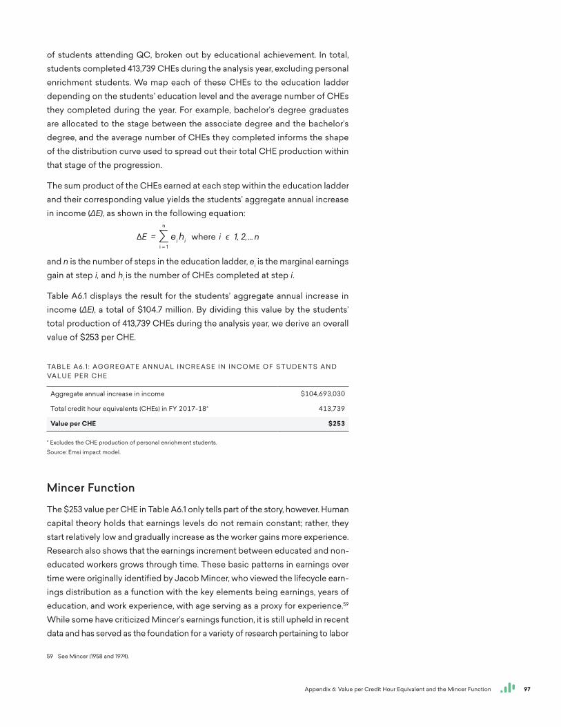
97Appendix 6: Value per Credit Hour Equivalent and the Mincer Function
of students attending QC, broken out by educational achievement. In total, students completed 413,739 CHEs during the analysis year, excluding personal enrichment students. We map each of these CHEs to the education ladder depending on the students’ education level and the average number of CHEs they completed during the year. For example, bachelor’s degree graduates are allocated to the stage between the associate degree and the bachelor’s degree, and the average number of CHEs they completed informs the shape of the distribution curve used to spread out their total CHE production within that stage of the progression.
The sum product of the CHEs earned at each step within the education ladder and their corresponding value yields the students’ aggregate annual increase in income (∆E), as shown in the following equation:
and n is the number of steps in the education ladder, ei is the marginal earnings gain at step i, and hi is the number of CHEs completed at step i.
Table A6.1 displays the result for the students’ aggregate annual increase in income (∆E), a total of $104.7 million. By dividing this value by the students’ total production of 413,739 CHEs during the analysis year, we derive an overall value of $253 per CHE.
Mincer Function
The $253 value per CHE in Table A6.1 only tells part of the story, however. Human capital theory holds that earnings levels do not remain constant; rather, they start relatively low and gradually increase as the worker gains more experience. Research also shows that the earnings increment between educated and non-educated workers grows through time. These basic patterns in earnings over time were originally identified by Jacob Mincer, who viewed the lifecycle earn-ings distribution as a function with the key elements being earnings, years of education, and work experience, with age serving as a proxy for experience.59 While some have criticized Mincer’s earnings function, it is still upheld in recent data and has served as the foundation for a variety of research pertaining to labor
59 See Mincer (1958 and 1974).
TA B L E A6.1 : AG G R E GAT E A N N UA L I N C R E AS E I N I N C O M E O F S T U D E N T S A N D VA L U E P E R C H E
Aggregate annual increase in income $104,693,030
Total credit hour equivalents (CHEs) in FY 2017-18* 413,739
Value per CHE $253
* Excludes the CHE production of personal enrichment students.
Source: Emsi impact model.
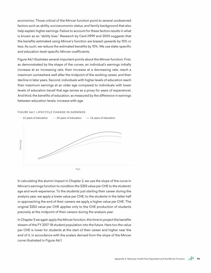
98Appendix 6: Value per Credit Hour Equivalent and the Mincer Function
economics. Those critical of the Mincer function point to several unobserved factors such as ability, socioeconomic status, and family background that also help explain higher earnings. Failure to account for these factors results in what is known as an “ability bias.” Research by Card (1999 and 2001) suggests that the benefits estimated using Mincer’s function are biased upwards by 10% or less. As such, we reduce the estimated benefits by 10%. We use state-specific and education level-specific Mincer coefficients.
Figure A6.1 illustrates several important points about the Mincer function. First, as demonstrated by the shape of the curves, an individual’s earnings initially increase at an increasing rate, then increase at a decreasing rate, reach a maximum somewhere well after the midpoint of the working career, and then decline in later years. Second, individuals with higher levels of education reach their maximum earnings at an older age compared to individuals with lower levels of education (recall that age serves as a proxy for years of experience). And third, the benefits of education, as measured by the difference in earnings between education levels, increase with age.
In calculating the alumni impact in Chapter 2, we use the slope of the curve in Mincer’s earnings function to condition the $253 value per CHE to the students’ age and work experience. To the students just starting their career during the analysis year, we apply a lower value per CHE; to the students in the latter half or approaching the end of their careers we apply a higher value per CHE. The original $253 value per CHE applies only to the CHE production of students precisely at the midpoint of their careers during the analysis year.
In Chapter 3 we again apply the Mincer function, this time to project the benefits stream of the FY 2017-18 student population into the future. Here too the value per CHE is lower for students at the start of their career and higher near the end of it, in accordance with the scalars derived from the slope of the Mincer curve illustrated in Figure A6.1.
F I G U R E A6.1 : L I F E C YC L E C H A N G E I N E A R N I N G S
Earn
ings
Age
12 years of education 14 years of education 16 years of education
99Appendix 7: Alternative Education Variable
Appendix 7: Alternative Education Variable
In a scenario where the college did not exist, some of its students would still be able to avail themselves of an alternative comparable education. These students create benefits in the region even in the absence of the college. The alternative education variable accounts for these students and is used to discount the benefits we attribute to the college.
Recall this analysis considers only relevant economic information regarding the college. Considering the existence of various other academic institutions surrounding the college, we have to assume that a portion of the students could find alternative education and either remain in or return to the region. For example, some students may participate in online programs while remaining in the region. Others may attend an out-of-region institution and return to the region upon completing their studies. For these students—who would have found an alternative education and produced benefits in the region regardless of the presence of the college—we discount the benefits attributed to the col-lege. An important distinction must be made here: the benefits from students who would find alternative education outside the region and not return to the region are not discounted. Because these benefits would not occur in the region without the presence of the college, they must be included.
In the absence of the college, we assume 15% of the college’s students would find alternative education opportunities and remain in or return to the region. We account for this by discounting the alumni impact, the benefits to taxpayers, and the benefits to society in the region in Chapters 2 and 3 by 15%. In other words, we assume 15% of the benefits created by the college’s students would have occurred anyway in the counterfactual scenario where the college did not exist. A sensitivity analysis of this adjustment is presented in Appendix 1.
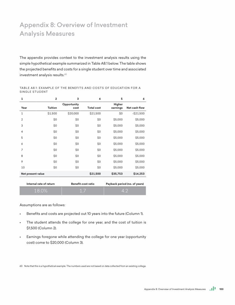
100Appendix 8: Overview of Investment Analysis Measures
Appendix 8: Overview of Investment Analysis Measures
The appendix provides context to the investment analysis results using the simple hypothetical example summarized in Table A8.1 below. The table shows the projected benefits and costs for a single student over time and associated investment analysis results.60
Assumptions are as follows:
• Benefits and costs are projected out 10 years into the future (Column 1).
• The student attends the college for one year, and the cost of tuition is $1,500 (Column 2).
• Earnings foregone while attending the college for one year (opportunity cost) come to $20,000 (Column 3).
60 Note that this is a hypothetical example. The numbers used are not based on data collected from an existing college.
TA B L E A8.1 : E X A M P L E O F T H E B E N E F I T S A N D C O S T S O F E D U CAT I O N F O R A S I N G L E S T U D E N T
1 2 3 4 5 6
Year TuitionOpportunity
cost Total costHigher
earnings Net cash flow
1 $1,500 $20,000 $21,500 $0 -$21,500
2 $0 $0 $0 $5,000 $5,000
3 $0 $0 $0 $5,000 $5,000
4 $0 $0 $0 $5,000 $5,000
5 $0 $0 $0 $5,000 $5,000
6 $0 $0 $0 $5,000 $5,000
7 $0 $0 $0 $5,000 $5,000
8 $0 $0 $0 $5,000 $5,000
9 $0 $0 $0 $5,000 $5,000
10 $0 $0 $0 $5,000 $5,000
Net present value $21,500 $35,753 $14,253
Internal rate of return Benefit-cost ratio Payback period (no. of years)
18.0% 1.7 4.2
101Appendix 8: Overview of Investment Analysis Measures
• Together, tuition and earnings foregone cost sum to $21,500. This rep-resents the out-of-pocket investment made by the student (Column 4).
• In return, the student earns $5,000 more per year than he otherwise would have earned without the education (Column 5).
• The net cash flow (NCF) in Column 6 shows higher earnings (Column 5) less the total cost (Column 4).
• The assumed going rate of interest is 4%, the rate of return from alternative investment schemes for the use of the $21,500.
Results are expressed in standard investment analysis terms, which are as fol-lows: the net present value, the internal rate of return, the benefit-cost ratio, and the payback period. Each of these is briefly explained below in the context of the cash flow numbers presented in Table A8.1.
Net present value
The student in Table A8.1 can choose either to attend college or to forego post-secondary education and maintain his present employment. If he decides to enroll, certain economic implications unfold. Tuition and fees must be paid, and earnings will cease for one year. In exchange, the student calculates that with post-secondary education, his earnings will increase by at least the $5,000 per year, as indicated in the table.
The question is simple: Will the prospective student be economically better off by choosing to enroll? If he adds up higher earnings of $5,000 per year for the remaining nine years in Table A8.1, the total will be $45,000. Compared to a total investment of $21,500, this appears to be a very solid investment. The reality, however, is different. Benefits are far lower than $45,000 because future money is worth less than present money. Costs (tuition plus earnings foregone) are felt immediately because they are incurred today, in the present. Benefits, on the other hand, occur in the future. They are not yet available. All future benefits must be discounted by the going rate of interest (referred to as the discount rate) to be able to express them in present value terms.61
Let us take a brief example. At 4%, the present value of $5,000 to be received one year from today is $4,807. If the $5,000 were to be received in year 10, the present value would reduce to $3,377. Put another way, $4,807 deposited in the bank today earning 4% interest will grow to $5,000 in one year; and $3,377 deposited today would grow to $5,000 in 10 years. An “economically rational” person would, therefore, be equally satisfied receiving $3,377 today or $5,000
61 Technically, the interest rate is applied to compounding – the process of looking at deposits today and determin-ing how much they will be worth in the future. The same interest rate is called a discount rate when the process is reversed – determining the present value of future earnings.
102Appendix 8: Overview of Investment Analysis Measures
10 years from today given the going rate of interest of 4%. The process of discounting—finding the present value of future higher earnings—allows the model to express values on an equal basis in future or present value terms.
The goal is to express all future higher earnings in present value terms so that they can be compared to investments incurred today (in this example, tuition plus earnings foregone). As indicated in Table A8.1 the cumulative present value of $5,000 worth of higher earnings between years 2 and 10 is $35,753 given the 4% interest rate, far lower than the undiscounted $45,000 discussed above.
The net present value of the investment is $14,253. This is simply the present value of the benefits less the present value of the costs, or $35,753 – $21,500 = $14,253. In other words, the present value of benefits exceeds the present value of costs by as much as $14,253. The criterion for an economically worthwhile investment is that the net present value is equal to or greater than zero. Given this result, it can be concluded that, in this case, and given these assumptions, this particular investment in education is very strong.
Internal rate of return
The internal rate of return is another way of measuring the worth of investing in education using the same cash flows shown in Table A8.1. In technical terms, the internal rate of return is a measure of the average earning power of money used over the life of the investment. It is simply the interest rate that makes the net present value equal to zero. In the discussion of the net present value above, the model applies the going rate of interest of 4% and computes a positive net present value of $14,253. The question now is what the interest rate would have to be in order to reduce the net present value to zero. Obviously it would have to be higher—18.0% in fact, as indicated in Table A8.1. Or, if a discount rate of 18.0% were applied to the net present value calculations instead of the 4%, then the net present value would reduce to zero.
What does this mean? The internal rate of return of 18.0% defines a breakeven solution—the point where the present value of benefits just equals the present value of costs, or where the net present value equals zero. Or, at 18.0%, higher earnings of $5,000 per year for the next nine years will earn back all invest-ments of $21,500 made plus pay 18.0% for the use of that money ($21,500) in the meantime. Is this a good return? Indeed, it is. If it is compared to the 4% going rate of interest applied to the net present value calculations, 18.0% is far higher than 4%. It may be concluded, therefore, that the investment in this case is solid. Alternatively, comparing the 18.0% rate of return to the long-term 10% rate or so obtained from investments in stocks and bonds also indicates that the investment in education is strong relative to the stock market returns (on average).
103Appendix 8: Overview of Investment Analysis Measures
Benefit-cost ratio
The benefit-cost ratio is simply the present value of benefits divided by pres-ent value of costs, or $35,753 ÷ $21,500 = 1.7 (based on the 4% discount rate). Of course, any change in the discount rate would also change the benefit-cost ratio. Applying the 18.0% internal rate of return discussed above would reduce the benefit-cost ratio to 1.0, the breakeven solution where benefits just equal costs. Applying a discount rate higher than the 18.0% would reduce the ratio to lower than 1.0, and the investment would not be feasible. The 1.7 ratio means that a dollar invested today will return a cumulative $1.70 over the ten-year time period.
Payback period
This is the length of time from the beginning of the investment (consisting of tuition and earnings foregone) until higher future earnings give a return on the investment made. For the student in Table A8.1, it will take roughly 4.2 years of $5,000 worth of higher earnings to recapture his investment of $1,500 in tuition and the $20,000 in earnings foregone while attending the college. Higher earnings that occur beyond 4.2 years are the returns that make the investment in education in this example economically worthwhile. The payback period is a fairly rough, albeit common, means of choosing between investments. The shorter the payback period, the stronger the investment.
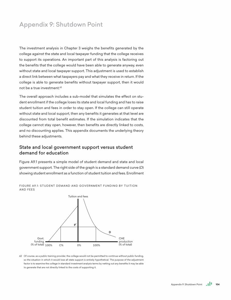
104Appendix 9: Shutdown Point
Appendix 9: Shutdown Point
The investment analysis in Chapter 3 weighs the benefits generated by the college against the state and local taxpayer funding that the college receives to support its operations. An important part of this analysis is factoring out the benefits that the college would have been able to generate anyway, even without state and local taxpayer support. This adjustment is used to establish a direct link between what taxpayers pay and what they receive in return. If the college is able to generate benefits without taxpayer support, then it would not be a true investment.62
The overall approach includes a sub-model that simulates the effect on stu-dent enrollment if the college loses its state and local funding and has to raise student tuition and fees in order to stay open. If the college can still operate without state and local support, then any benefits it generates at that level are discounted from total benefit estimates. If the simulation indicates that the college cannot stay open, however, then benefits are directly linked to costs, and no discounting applies. This appendix documents the underlying theory behind these adjustments.
State and local government support versus student demand for education
Figure A9.1 presents a simple model of student demand and state and local government support. The right side of the graph is a standard demand curve (D) showing student enrollment as a function of student tuition and fees. Enrollment
62 Of course, as a public training provider, the college would not be permitted to continue without public funding, so the situation in which it would lose all state support is entirely hypothetical. The purpose of the adjustment factor is to examine the college in standard investment analysis terms by netting out any benefits it may be able to generate that are not directly linked to the costs of supporting it.
F I G U R E A9.1 : S T U D E N T D E M A N D A N D G OV E R N M E N T F U N D I N G BY T U I T I O N A N D F E E S
Tuition and fees
CHE production (% of total)100% C% 0% 100%
D
p'
Govt. funding
(% of total)
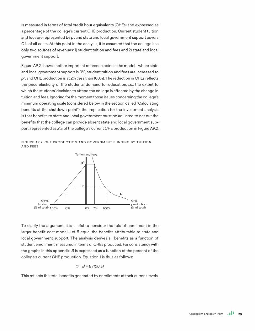
105Appendix 9: Shutdown Point
is measured in terms of total credit hour equivalents (CHEs) and expressed as a percentage of the college’s current CHE production. Current student tuition and fees are represented by p’, and state and local government support covers C% of all costs. At this point in the analysis, it is assumed that the college has only two sources of revenues: 1) student tuition and fees and 2) state and local government support.
Figure A9.2 shows another important reference point in the model—where state and local government support is 0%, student tuition and fees are increased to p’’, and CHE production is at Z% (less than 100%). The reduction in CHEs reflects the price elasticity of the students’ demand for education, i.e., the extent to which the students’ decision to attend the college is affected by the change in tuition and fees. Ignoring for the moment those issues concerning the college’s minimum operating scale (considered below in the section called “Calculating benefits at the shutdown point”), the implication for the investment analysis is that benefits to state and local government must be adjusted to net out the benefits that the college can provide absent state and local government sup-port, represented as Z% of the college’s current CHE production in Figure A9.2.
To clarify the argument, it is useful to consider the role of enrollment in the larger benefit-cost model. Let B equal the benefits attributable to state and local government support. The analysis derives all benefits as a function of student enrollment, measured in terms of CHEs produced. For consistency with the graphs in this appendix, B is expressed as a function of the percent of the college’s current CHE production. Equation 1 is thus as follows:
1) B = B (100%)
This reflects the total benefits generated by enrollments at their current levels.
F I G U R E A9.2: C H E P R O D U C T I O N A N D G OV E R N M E N T F U N D I N G BY T U I T I O N A N D F E E S
Tuition and fees
CHE production (% of total)100% C% 0% 100%Z%
D
p'
p"
Govt. funding
(% of total)
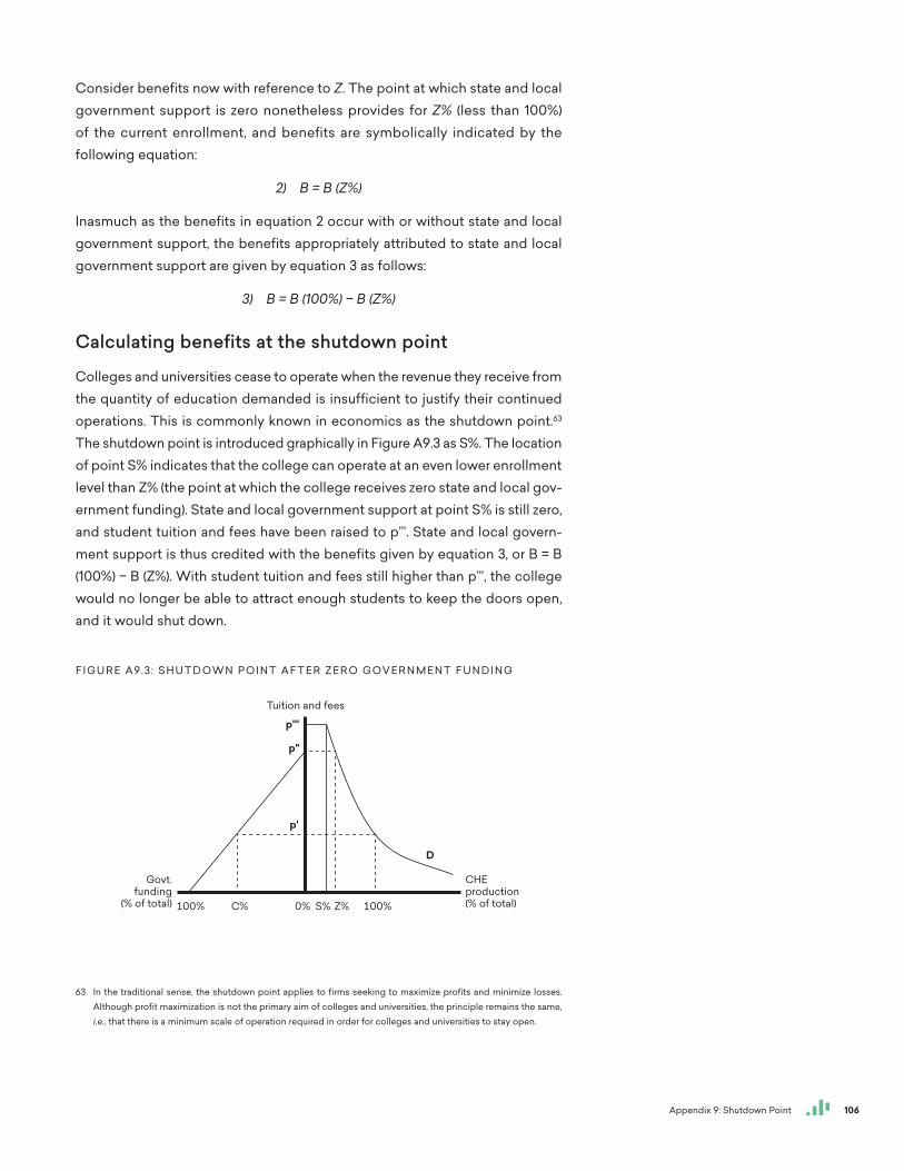
106Appendix 9: Shutdown Point
Consider benefits now with reference to Z. The point at which state and local government support is zero nonetheless provides for Z% (less than 100%) of the current enrollment, and benefits are symbolically indicated by the following equation:
2) B = B (Z%)
Inasmuch as the benefits in equation 2 occur with or without state and local government support, the benefits appropriately attributed to state and local government support are given by equation 3 as follows:
3) B = B (100%) − B (Z%)
Calculating benefits at the shutdown point
Colleges and universities cease to operate when the revenue they receive from the quantity of education demanded is insufficient to justify their continued operations. This is commonly known in economics as the shutdown point.63 The shutdown point is introduced graphically in Figure A9.3 as S%. The location of point S% indicates that the college can operate at an even lower enrollment level than Z% (the point at which the college receives zero state and local gov-ernment funding). State and local government support at point S% is still zero, and student tuition and fees have been raised to p’’’. State and local govern-ment support is thus credited with the benefits given by equation 3, or B = B (100%) − B (Z%). With student tuition and fees still higher than p’’’, the college would no longer be able to attract enough students to keep the doors open, and it would shut down.
63 In the traditional sense, the shutdown point applies to firms seeking to maximize profits and minimize losses. Although profit maximization is not the primary aim of colleges and universities, the principle remains the same, i.e., that there is a minimum scale of operation required in order for colleges and universities to stay open.
F I G U R E A9.3: S H U T D OW N P O I N T A F T E R Z E R O G OV E R N M E N T F U N D I N G
Tuition and fees
CHE production (% of total)100% C% Z%0% S% 100%
D
p'
p"
p'''
Govt. funding
(% of total)
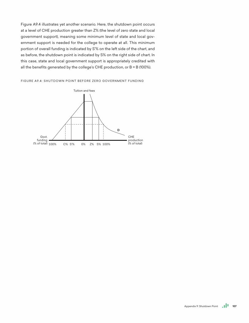
107Appendix 9: Shutdown Point
Figure A9.4 illustrates yet another scenario. Here, the shutdown point occurs at a level of CHE production greater than Z% (the level of zero state and local government support), meaning some minimum level of state and local gov-ernment support is needed for the college to operate at all. This minimum portion of overall funding is indicated by S’% on the left side of the chart, and as before, the shutdown point is indicated by S% on the right side of chart. In this case, state and local government support is appropriately credited with all the benefits generated by the college’s CHE production, or B = B (100%).
F I G U R E A9.4: S H U T D OW N P O I N T B E F O R E Z E R O G OV E R N M E N T F U N D I N G
Tuition and fees
CHE production (% of total)100% C% S'% Z%0% S% 100%
D
Govt. funding
(% of total)
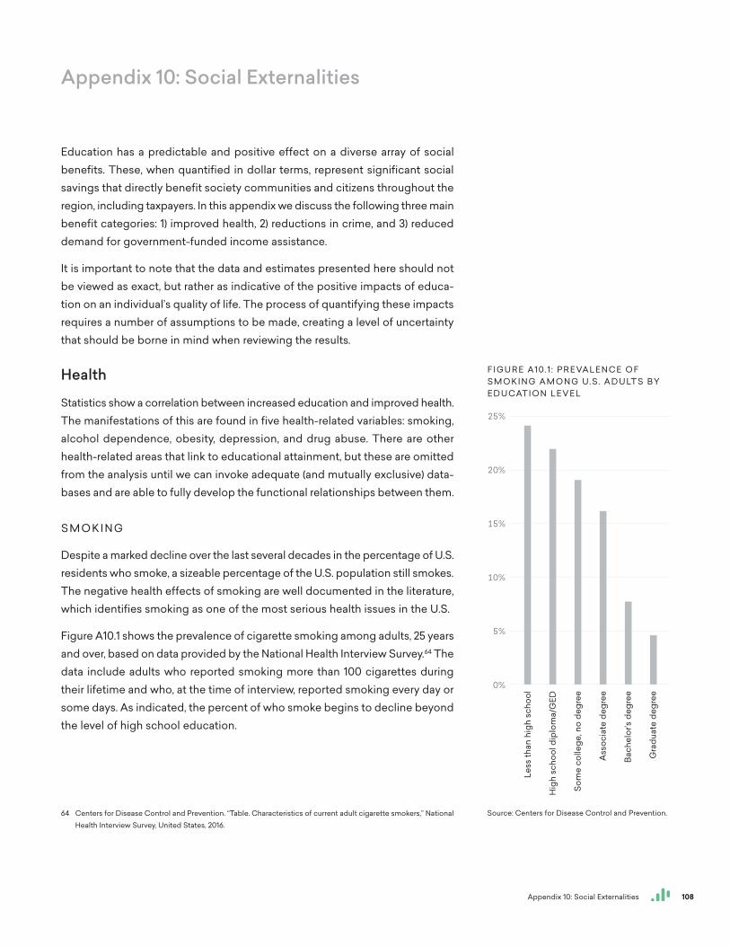
108Appendix 10: Social Externalities
Appendix 10: Social Externalities
Education has a predictable and positive effect on a diverse array of social benefits. These, when quantified in dollar terms, represent significant social savings that directly benefit society communities and citizens throughout the region, including taxpayers. In this appendix we discuss the following three main benefit categories: 1) improved health, 2) reductions in crime, and 3) reduced demand for government-funded income assistance.
It is important to note that the data and estimates presented here should not be viewed as exact, but rather as indicative of the positive impacts of educa-tion on an individual’s quality of life. The process of quantifying these impacts requires a number of assumptions to be made, creating a level of uncertainty that should be borne in mind when reviewing the results.
Health
Statistics show a correlation between increased education and improved health. The manifestations of this are found in five health-related variables: smoking, alcohol dependence, obesity, depression, and drug abuse. There are other health-related areas that link to educational attainment, but these are omitted from the analysis until we can invoke adequate (and mutually exclusive) data-bases and are able to fully develop the functional relationships between them.
S M O K I N G
Despite a marked decline over the last several decades in the percentage of U.S. residents who smoke, a sizeable percentage of the U.S. population still smokes. The negative health effects of smoking are well documented in the literature, which identifies smoking as one of the most serious health issues in the U.S.
Figure A10.1 shows the prevalence of cigarette smoking among adults, 25 years and over, based on data provided by the National Health Interview Survey.64 The data include adults who reported smoking more than 100 cigarettes during their lifetime and who, at the time of interview, reported smoking every day or some days. As indicated, the percent of who smoke begins to decline beyond the level of high school education.
64 Centers for Disease Control and Prevention. “Table. Characteristics of current adult cigarette smokers,” National Health Interview Survey, United States, 2016.
F I G U R E A10.1 : P R E VA L E N C E O F S M O K I N G A M O N G U. S. A D U LT S BY E D U CAT I O N L E V E L
25%
20%
15%
10%
5%
0%
Less
than
hig
h sc
hool
Hig
h sc
hool
dip
lom
a/G
ED
Som
e co
llege
, no
degr
ee
Ass
ocia
te d
egre
e
Bac
helo
r’s d
egre
e
Gra
duat
e de
gree
Source: Centers for Disease Control and Prevention.
100 + 91 + 79 + 67 + 32 + 19
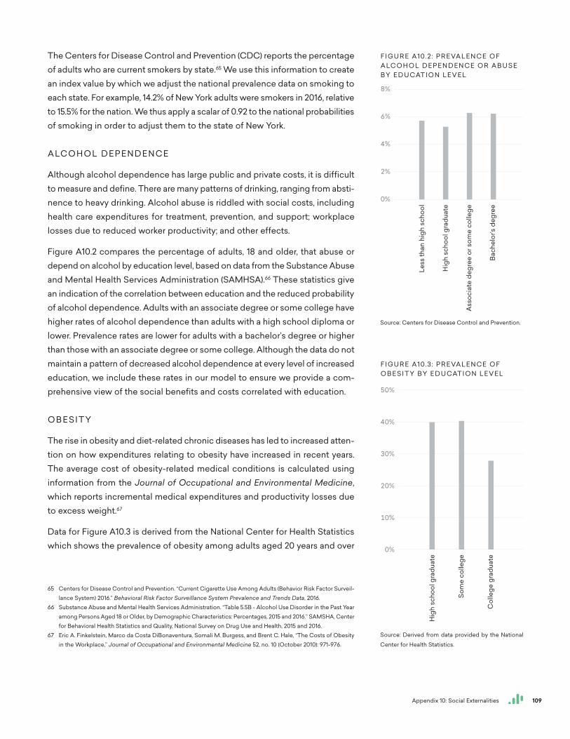
109Appendix 10: Social Externalities
The Centers for Disease Control and Prevention (CDC) reports the percentage of adults who are current smokers by state.65 We use this information to create an index value by which we adjust the national prevalence data on smoking to each state. For example, 14.2% of New York adults were smokers in 2016, relative to 15.5% for the nation. We thus apply a scalar of 0.92 to the national probabilities of smoking in order to adjust them to the state of New York.
A LC O H O L D E P E N D E N C E
Although alcohol dependence has large public and private costs, it is difficult to measure and define. There are many patterns of drinking, ranging from absti-nence to heavy drinking. Alcohol abuse is riddled with social costs, including health care expenditures for treatment, prevention, and support; workplace losses due to reduced worker productivity; and other effects.
Figure A10.2 compares the percentage of adults, 18 and older, that abuse or depend on alcohol by education level, based on data from the Substance Abuse and Mental Health Services Administration (SAMHSA).66 These statistics give an indication of the correlation between education and the reduced probability of alcohol dependence. Adults with an associate degree or some college have higher rates of alcohol dependence than adults with a high school diploma or lower. Prevalence rates are lower for adults with a bachelor’s degree or higher than those with an associate degree or some college. Although the data do not maintain a pattern of decreased alcohol dependence at every level of increased education, we include these rates in our model to ensure we provide a com-prehensive view of the social benefits and costs correlated with education.
O B E S I T Y
The rise in obesity and diet-related chronic diseases has led to increased atten-tion on how expenditures relating to obesity have increased in recent years. The average cost of obesity-related medical conditions is calculated using information from the Journal of Occupational and Environmental Medicine, which reports incremental medical expenditures and productivity losses due to excess weight.67
Data for Figure A10.3 is derived from the National Center for Health Statistics which shows the prevalence of obesity among adults aged 20 years and over
65 Centers for Disease Control and Prevention. “Current Cigarette Use Among Adults (Behavior Risk Factor Surveil-lance System) 2016.” Behavioral Risk Factor Surveillance System Prevalence and Trends Data, 2016.
66 Substance Abuse and Mental Health Services Administration. “Table 5.5B - Alcohol Use Disorder in the Past Year among Persons Aged 18 or Older, by Demographic Characteristics: Percentages, 2015 and 2016.” SAMSHA, Center for Behavioral Health Statistics and Quality, National Survey on Drug Use and Health, 2015 and 2016.
67 Eric A. Finkelstein, Marco da Costa DiBonaventura, Somali M. Burgess, and Brent C. Hale, “The Costs of Obesity in the Workplace,” Journal of Occupational and Environmental Medicine 52, no. 10 (October 2010): 971-976.
F I G U R E A10.2: P R E VA L E N C E O F A LC O H O L D E P E N D E N C E O R A B U S E BY E D U CAT I O N L E V E L
F I G U R E A10.3: P R E VA L E N C E O F O B E S I T Y BY E D U CAT I O N L E V E L
50%
20%
10%
0%
40%
30%
Source: Centers for Disease Control and Prevention.
Source: Derived from data provided by the National
Center for Health Statistics.
Less
than
hig
h sc
hool
Hig
h sc
hool
gra
duat
e
Ass
ocia
te d
egre
e or
som
e co
llege
Bac
helo
r’s d
egre
e
Hig
h sc
hool
gra
duat
e
Som
e co
llege
Col
lege
gra
duat
e
8%
2%
0%
4%
6%
99 + 100 + 69
91 + 84 + 100 + 99
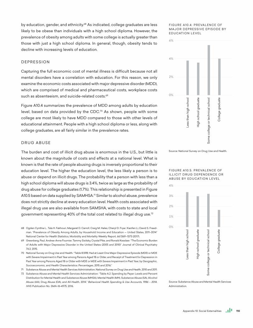
110Appendix 10: Social Externalities
by education, gender, and ethnicity.68 As indicated, college graduates are less likely to be obese than individuals with a high school diploma. However, the prevalence of obesity among adults with some college is actually greater than those with just a high school diploma. In general, though, obesity tends to decline with increasing levels of education.
D E P R E S S I O N
Capturing the full economic cost of mental illness is difficult because not all mental disorders have a correlation with education. For this reason, we only examine the economic costs associated with major depressive disorder (MDD), which are comprised of medical and pharmaceutical costs, workplace costs such as absenteeism, and suicide-related costs.69
Figure A10.4 summarizes the prevalence of MDD among adults by education level, based on data provided by the CDC.70 As shown, people with some college are most likely to have MDD compared to those with other levels of educational attainment. People with a high school diploma or less, along with college graduates, are all fairly similar in the prevalence rates.
D R U G A B U S E
The burden and cost of illicit drug abuse is enormous in the U.S., but little is known about the magnitude of costs and effects at a national level. What is known is that the rate of people abusing drugs is inversely proportional to their education level. The higher the education level, the less likely a person is to abuse or depend on illicit drugs. The probability that a person with less than a high school diploma will abuse drugs is 3.4%, twice as large as the probability of drug abuse for college graduates (1.7%). This relationship is presented in Figure A10.5 based on data supplied by SAMHSA.71 Similar to alcohol abuse, prevalence does not strictly decline at every education level. Health costs associated with illegal drug use are also available from SAMSHA, with costs to state and local government representing 40% of the total cost related to illegal drug use.72
68 Ogden Cynthia L., Tala H. Fakhouri, Margaret D. Carroll, Craig M. Hales, Cheryl D. Fryar, Xianfen Li, David S. Freed-man. “Prevalence of Obesity Among Adults, by Household Income and Education — United States, 2011–2014” National Center for Health Statistics, Morbidity and Mortality Weekly Report, 66:1369–1373 (2017).
69 Greenberg, Paul, Andree-Anne Fournier, Tammy Sisitsky, Crystal Pike, and Ronald Kesslaer. “The Economic Burden of Adults with Major Depressive Disorder in the United States (2005 and 2010)” Journal of Clinical Psychiatry 76:2, 2015.
70 National Survey on Drug Use and Health. “Table 8.59B: Had at Least One Major Depressive Episode (MDE) or MDE with Severe Impairment in Past Year among Persons Aged 18 or Older, and Receipt of Treatment for Depression in Past Year among Persons Aged 18 or Older with MDE or MDE with Severe Impairment in Past Year, by Geographic, Socioeconomic, and Health Characteristics: Percentages, 2015 and 2016.”
71 Substance Abuse and Mental Health Services Administration, National Survey on Drug Use and Health, 2010 and 2011.72 Substance Abuse and Mental Health Services Administration. “Table A.2. Spending by Payer: Levels and Percent
Distribution for Mental Health and Substance Abuse (MHSA), Mental Health (MH), Substance Abuse (SA), Alcohol Abuse (AA), Drug Abuse (DA), and All-Health, 2014.” Behavioral Health Spending & Use Accounts, 1986 – 2014. HHS Publication No. SMA-16-4975, 2016.
F I G U R E A10.4: P R E VA L E N C E O F M A J O R D E P R E S S I V E E P I S O D E BY E D U CAT I O N L E V E L
F I G U R E A10.5: P R E VA L E N C E O F I L L I C I T D R U G D E P E N D E N C E O R A B U S E BY E D U CAT I O N L E V E L
Source: National Survey on Drug Use and Health.
Source: Substance Abuse and Mental Health Services
Administration.
Less
than
hig
h sc
hool
Hig
h sc
hool
gra
duat
e
Som
e co
llege
or t
echn
ical
sch
ool
Col
lege
gra
duat
e
Less
than
hig
h sc
hool
Hig
h sc
hool
gra
duat
e
Som
e co
llege
or t
echn
ical
sch
ool
Col
lege
gra
duat
e
2%
0%
4%
6%
2%
0%
4%
3%
1% 100 + 88 + 95 + 49
69 + 65 + 100 + 73
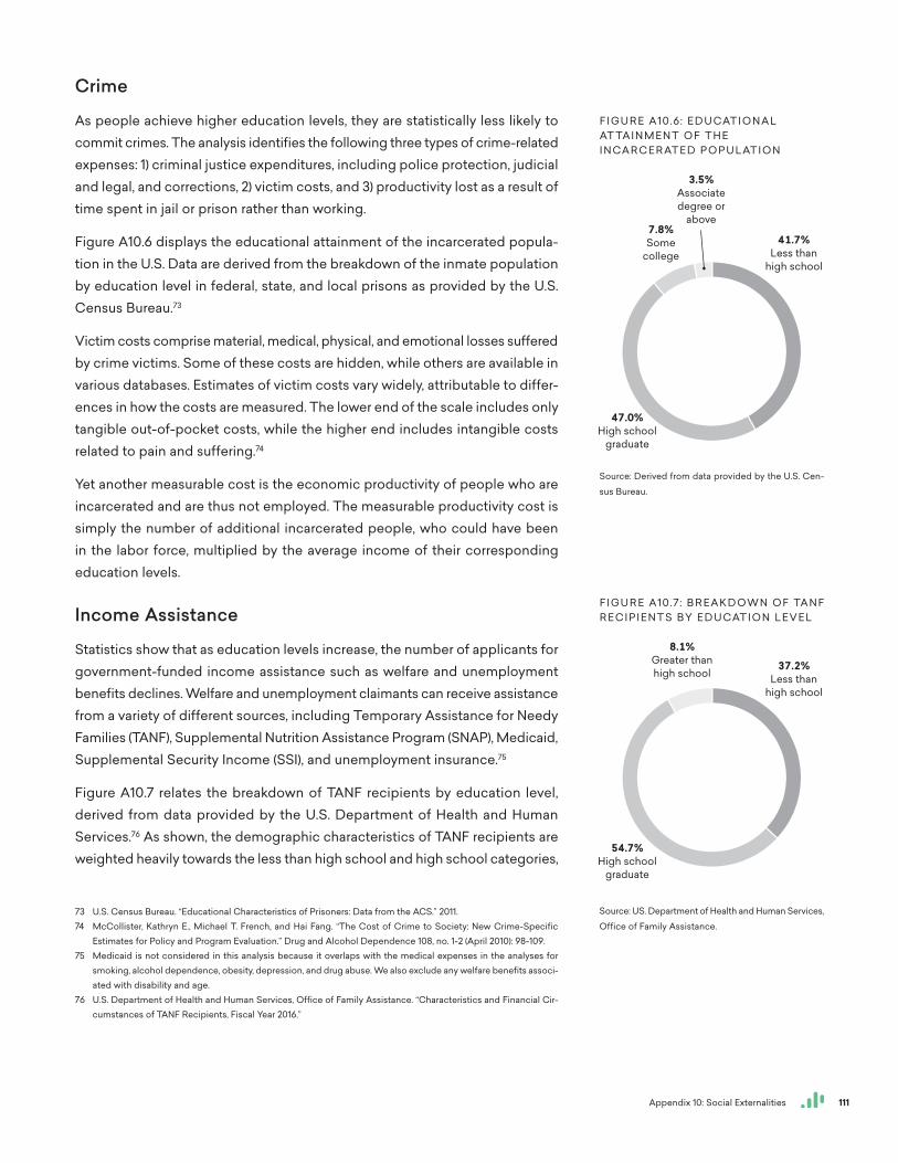
111Appendix 10: Social Externalities
Crime
As people achieve higher education levels, they are statistically less likely to commit crimes. The analysis identifies the following three types of crime-related expenses: 1) criminal justice expenditures, including police protection, judicial and legal, and corrections, 2) victim costs, and 3) productivity lost as a result of time spent in jail or prison rather than working.
Figure A10.6 displays the educational attainment of the incarcerated popula-tion in the U.S. Data are derived from the breakdown of the inmate population by education level in federal, state, and local prisons as provided by the U.S. Census Bureau.73
Victim costs comprise material, medical, physical, and emotional losses suffered by crime victims. Some of these costs are hidden, while others are available in various databases. Estimates of victim costs vary widely, attributable to differ-ences in how the costs are measured. The lower end of the scale includes only tangible out-of-pocket costs, while the higher end includes intangible costs related to pain and suffering.74
Yet another measurable cost is the economic productivity of people who are incarcerated and are thus not employed. The measurable productivity cost is simply the number of additional incarcerated people, who could have been in the labor force, multiplied by the average income of their corresponding education levels.
Income Assistance
Statistics show that as education levels increase, the number of applicants for government-funded income assistance such as welfare and unemployment benefits declines. Welfare and unemployment claimants can receive assistance from a variety of different sources, including Temporary Assistance for Needy Families (TANF), Supplemental Nutrition Assistance Program (SNAP), Medicaid, Supplemental Security Income (SSI), and unemployment insurance.75
Figure A10.7 relates the breakdown of TANF recipients by education level, derived from data provided by the U.S. Department of Health and Human Services.76 As shown, the demographic characteristics of TANF recipients are weighted heavily towards the less than high school and high school categories,
73 U.S. Census Bureau. “Educational Characteristics of Prisoners: Data from the ACS.” 2011.74 McCollister, Kathryn E., Michael T. French, and Hai Fang. “The Cost of Crime to Society: New Crime-Specific
Estimates for Policy and Program Evaluation.” Drug and Alcohol Dependence 108, no. 1-2 (April 2010): 98-109.75 Medicaid is not considered in this analysis because it overlaps with the medical expenses in the analyses for
smoking, alcohol dependence, obesity, depression, and drug abuse. We also exclude any welfare benefits associ-ated with disability and age.
76 U.S. Department of Health and Human Services, Office of Family Assistance. “Characteristics and Financial Cir-cumstances of TANF Recipients, Fiscal Year 2016.”
F I G U R E A10.6: E D U CAT I O N A L AT TA I N M E N T O F T H E I N CA R C E R AT E D P O P U L AT I O N
F I G U R E A10.7: B R E A K D OW N O F TA N F R E C I P I E N T S BY E D U CAT I O N L E V E L
4242+4747+88+33+R
3737+5555+88+R
41.7%Less than
high school
37.2%Less than
high school
47.0%High school
graduate
54.7%High school
graduate
7.8%Some
college
3.5%Associate degree or
above
8.1%Greater than high school
Source: Derived from data provided by the U.S. Cen-
sus Bureau.
Source: US. Department of Health and Human Services,
Office of Family Assistance.
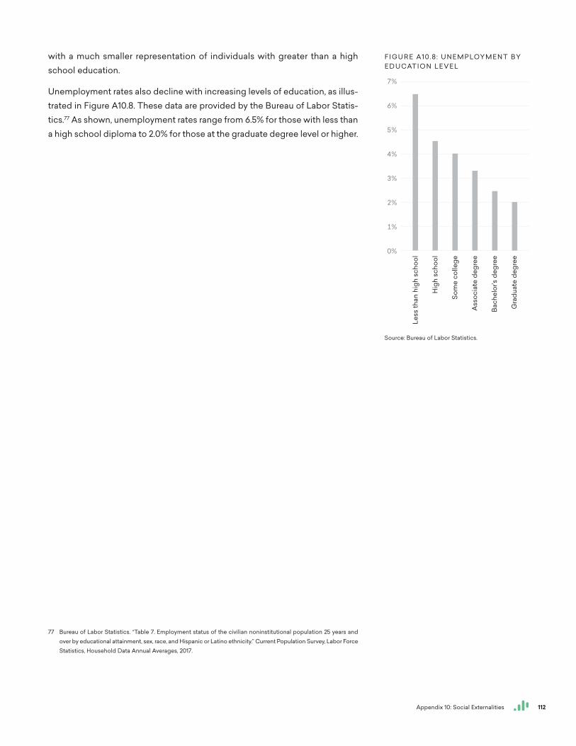
112Appendix 10: Social Externalities
with a much smaller representation of individuals with greater than a high school education.
Unemployment rates also decline with increasing levels of education, as illus-trated in Figure A10.8. These data are provided by the Bureau of Labor Statis-tics.77 As shown, unemployment rates range from 6.5% for those with less than a high school diploma to 2.0% for those at the graduate degree level or higher.
77 Bureau of Labor Statistics. “Table 7. Employment status of the civilian noninstitutional population 25 years and over by educational attainment, sex, race, and Hispanic or Latino ethnicity.” Current Population Survey, Labor Force Statistics, Household Data Annual Averages, 2017.
F I G U R E A10.8: U N E M P LOY M E N T BY E D U CAT I O N L E V E L
Source: Bureau of Labor Statistics.
Less
than
hig
h sc
hool
Hig
h sc
hool
Som
e co
llege
Ass
ocia
te d
egre
e
Bac
helo
r’s d
egre
e
Gra
duat
e de
gree
7%
6%
5%
4%
0%
3%
2%
1% 100 + 70 + 62 + 51 + 38 + 31