MATHEMATICAL ENGINEERINGTECHNICAL REPORTS

Markov Degree of the Three-State ToricHomogeneous Markov Chain Model

David HAWS, Abraham MARTIN DEL CAMPO,Akimichi TAKEMURA and Ruriko YOSHIDA

METR 2012–09 May 2012

DEPARTMENT OF MATHEMATICAL INFORMATICSGRADUATE SCHOOL OF INFORMATION SCIENCE AND TECHNOLOGY

THE UNIVERSITY OF TOKYOBUNKYO-KU, TOKYO 113-8656, JAPAN

WWW page: http://www.keisu.t.u-tokyo.ac.jp/research/techrep/index.html

The METR technical reports are published as a means to ensure timely dissemination of

scholarly and technical work on a non-commercial basis. Copyright and all rights therein

are maintained by the authors or by other copyright holders, notwithstanding that they

have offered their works here electronically. It is understood that all persons copying this

information will adhere to the terms and constraints invoked by each author’s copyright.

These works may not be reposted without the explicit permission of the copyright holder.

Markov degree of the three-state toric homogeneous Markov chain model

David Haws, Abraham Martın del Campo, Akimichi Takemura, Ruriko Yoshida∗

University of Kentucky, Department of Statistics

Abstract

Markov chain models had proved to be useful tools in many fields, such as physics, chemistry,information sciences, economics, finances, mathematical biology, social sciences, and statisticsfor analyzing data. A discrete time Markov chain is often used as a statistical model froma random physical process to fit the observed data. A time-homogeneous Markov chain is aprocess that each transition probability from a state to a state does not depend on time. Itis important to test if the assumption of the time-homogeneity of the chain fits the observeddata. In 2011, Hara and Takemura suggested a Markov Chain Monte Carlo (MCMC) approachto a goodness-of-fit test using Markov bases on the toric homogeneous Markov chain (THMC)model and gave a full description of the Markov bases for the two-state THMC model which doesnot depend on time T . In this paper, we provide a bound on the degree of the Markov basesfor the three-state THMC model (without loops and initial parameters), when the transitionprobabilities of the Markov chains are assumed to be independent of the time. Our proof isbased on a result due to Sturmfels, who gave a bound on the degree for the generators of toricideals, provided the normality of the corresponding toric variety. In our setting, we proved thenormality of the semigroup generated by the columns of the design matrix associated to theTHMC model by studying the geometric properties of the polytope associated to the designmatrix of the model. Moreover, we give a complete description of the facets of this polytope,which does not depend on the time.

Keywords: Markov bases, toric homogeneous Markov chains, polyhedrons, semigroups

1. Introduction

A discrete time Markov chain, Xt for t = 1, 2, . . ., is a stochastic process with the Markovproperty, that is P (Xt+1 = y|X1 = x1, . . . , Xt−1 = xt−1, Xt = x) = P (Xt+1 = y|Xt = x) forany states x, y. Discrete time Markov chains have applications in several fields, such as physics,chemistry, information sciences, economics, finances, mathematical biology, social sciences, andstatistics [8]. In this paper, we consider a discrete time Markov chain Xt, with t = 1, . . . , T(T ≥ 3), over a finite set of states [S] = {1, . . . , S}. In this paper we focus on S = 3.

Discrete time Markov chains are often used in statistical models to fit the observed datafrom a random physical process. Sometimes, in order to simplify the model, it is convenient toconsider time-homogeneous Markov chains, where the transition probabilities do not depend onthe time, in other words, when

P (Xt+1 = y|Xt = x) = P (X2 = y|X1 = x) for all states x, y and for any t = 1 . . . , T.

∗ruriko.yoshida@uky.edu

Preprint submitted to Elsevier May 7, 2012

In order for a statistical model to reflect the observed data, it is necessary to verify if themodel fits the date via the goodness-of-fit test. For instance, for the time-homogeneous Markovchain model, it is necessary to test if the assumption of time-homogeneity fits the observed data.In this paper, we study some properties of these algebraic relations for the toric homogeneousMarkov chain (THMC) model, which is a slight generalization of the time-homogeneous Markovchain model, and which we explain as follows.

Let w = s1 · · · sT denote a word of length T on states [S]. Let p(w) denote the likelihoodof observing the word w. Since the time-homogeneous Markov chain model assumes that thetransition probabilities do not depend on time, we can write the likelihood as the product ofprobabilities

p(w) = πs1ps1,s2 · · · psT−1,sT , (1.1)

where, πsi indicates the initial distribution at the first state, and psi,sj are the transition prob-abilities from state si to sj . In usual time-homogeneous Markov chain model it is assumed

that the row sums of the transition probabilities are one:∑S

j=1 pi,j = 1, ∀i ∈ [S]. On theother hand, in the toric homogeneous Markov model (1.1), the parameters pi,j are free and wedo not assume that the row sums of the transition probabilities are one. This simplifies themodel as we can disregard some information from it. Also in many cases the parameters πs1for the initial distribution are known, or sometimes these parameters are all constant, namelyπ1 = π2 = · · · = πS = c; in this situation it is no longer necessary to take them in considerationfor the model. Another simplification that arises from practice is when the only transition prob-abilities considered are those between two different states, i.e. when pi,j = 0 whenever i = j;this situation is referred as the THMC model without self-loops.

In [11], Takemura and Hara suggested a Markov Chain Monte Carlo (MCMC) approach forthe goodness-of-fit test using Markov bases of the THMC model. A Markov basis is a set of movesbetween data sets with the same sufficient statistics so that the transition graph for the MCMCis guaranteed to be connected for any observed value of the sufficient statistics (see Section 2.1and [8]). A Markov basis can be encoded by polynomial relations among the probabilities pi,j .The set of all these algebraic relations is the toric ideal associated to the model.

In [11], the authors provided a full description of the Markov bases for the THMC modelin two states (i.e. when S = 2) that does not depend on T . Inspired by their work, we studythe algebraic and polyhedral properties of the Markov bases of the three-state THMC modelwithout initial parameters and without self-loops for any time T ≥ 3. As a result, we provedthat the Markov bases of the model consist of binomials of degree at most 6. Our proof relies onthe normality of the semigroup generated by the columns of the design matrix for the three-stateTHMC model for any time T ≥ 3, which we settle using a complete description of the facets ofthe convex hull generated by the columns of the design matrix.

The outline of this paper is as follows. In Section 2, we recall some definitions from Markovbases theory. In Section 3, we explicitly describe the hyperplane representation of the convexhull generated by the columns of the design matrix for the three-state THMC model for any timeT ≥ 4. Then, in Section 4 we show the normality of the semigroup generated by the columnsof the design matrix for the three-state THMC model for any time T ≥ 3. Finally, using theseresults, we present the proof of our bound on the degree of the Markov basis in Section 5,and we finalize that section with some observations based on the analysis of our computationalexperiments.

2

2. Notation

Let 〈S〉T be the set of all words of length T on states [S] such that every word has no self-loops; that is, if w = (s1, . . . , sT ) ∈ 〈S〉T then si 6= si+1 for i = 1, . . . , T −1. We define P∗(〈S〉T )to be the set of all multisets of words in 〈S〉T .

Let V(〈S〉T

)be the real vector space with basis 〈S〉T and note that V

(〈S〉T

) ∼= RS(S−1)T .We recall some definitions from the book of Pachter and Sturmfels [7]. Let A = (aij) be anon-negative integer d×m matrix with the property that all column sums are equal:

d∑i=1

ai1 =d∑i=1

ai2 = · · · =d∑i=1

aim.

Write A = [a1 a2 · · · am] where aj are the column vectors of A and define θaj =∏di=1 θ

aiji for

j = 1, . . . ,m. The toric model of A is the image of the orthant Rd≥0 under the map

f : Rd → Rm, θ 7→ 1∑mj=1 θ

aj(θa1 , . . . , θam) .

Here we have d parameters θ = (θ1, . . . , θd) and a discrete state space of size m. In our setting,the discrete space will be the set of all possible words on [S] of length T without self-loops (〈S〉T )and we can think of θ1, . . . , θd as the probabilities p1,2, p1,3, . . . , pS−1,S .

In this paper, we focus on the THMC model without initial parameters and with no self-loopsin three states, (i.e., S = 3), which is parametrized by 6 positive real variables: p12, p13, p21, p23,p31, p3,2. Thus, the number of parameters is d = 6 and the size of the discrete space is m = 6T−1,which is precisely the number of words in 〈3〉T . The model we study is thus the toric modelrepresented by the 6 × 6T−1 matrix AT , which will be referred to as the design matrix for themodel on 3 states with time T . The rows of AT are indexed by elements in 〈3〉2 and the columnsare indexed by words in 〈3〉T . The entry of AT indexed by row σ1σ2 ∈ 〈3〉2, and column w =(s1, . . . , sT ) ∈ 〈3〉T is equal to the cardinality of the set { i ∈ {1, . . . , T − 1} | σ1σ2 = sisi+1 }.

Example 2.1. Ordering 〈3〉2 and 〈3〉T lexicographically, and letting T = 4, the matrix A4 is:

1212

1213

1231

1232

1312

1313

1321

1323

2121

2123

2131

2132

2312

2313

2321

2323

3121

3123

3131

3132

3212

3213

3231

3232

12 2 1 1 1 1 0 0 0 1 1 1 0 0 0 0 0 1 1 1 0 0 0 0 013 0 1 1 0 0 2 1 1 0 0 0 1 1 1 0 0 0 0 0 1 1 1 0 021 1 1 0 0 0 0 1 0 2 1 0 1 1 0 1 0 1 1 0 1 0 0 0 023 0 0 0 1 1 0 0 1 0 1 1 0 0 1 1 2 0 0 1 0 0 0 1 131 0 0 1 1 0 1 0 0 0 0 1 1 0 1 0 0 1 0 1 0 2 1 1 032 0 0 0 0 1 0 1 1 0 0 0 0 1 0 1 1 0 1 0 1 0 1 1 2

2.1. Sufficient statistics, ideals, and Markov basis

Let AT be the design matrix for the THMC model without initial parameters and with noself-loops. The column of AT indexed by w ∈ 〈3〉T is denoted by aTw. Thus, by extendinglinearly, the map AT : V(〈3〉T )→ R6 is well-defined.

Let W = {w1, . . . , wN} ∈ P∗(〈3〉T ) where we regard W as observed data which can be

summarized in the data vector u ∈ N6T−1. We index u by words in 〈3〉T , so the coordinate

representing for the word w in the vector u is denoted by uw, and its value is the number ofwords in W equal to w. Note since AT is linear then ATu is well-defined. We also adopt the

3

notation AT (W ) := ATu. For W from P∗(〈3〉T ), let u be its data vector, the sufficient statisticsfor the model are stored in the vector ATu. Often the data vector u is also referred to as acontingency table, in which case ATu is referred to as the marginals.

The design matrix AT above defines a toric ideal which is of central interest in this paper,as their set of generators are in bijection with the Markov bases. The toric ideal IAT is definedas the kernel of the homomorphism of polynomial rings ψ : C[{ p(w) | w ∈ 〈S〉T }] → C[{ pij |i, j ∈ [3], i 6= j }] defined by ψ(p(w)) = ps1,s2 · · · psT−1,sT , where { p(w) | w ∈ 〈S〉T } is regardedas a set of indeterminates.

The set of all contingency tables (data vectors) satisfying a given set of marginals b ∈ Zd≥0 is

called a fiber which we denote by Fb = {x ∈ Zm≥0 | AT (x) = b }. A move z ∈ Zm is an integer

vector satisfying AT (z) = 0. A Markov basis for our model defined by the design matrix AT isdefined as a finite set Z of moves satisfying that for all b and all pairs x,y ∈ Fb there exists asequence z1, . . . , zK ∈ Z such that

y = x +

K∑k=1

zk, with x +

l∑k=1

zk ≥ 0, for all l = 1, . . . ,K.

A minimal Markov basis is a Markov basis which is minimal in terms of inclusion. See Diaconisand Sturmfels[2] for more details on Markov bases and their toric ideals.

2.2. State Graph

We give here a useful tool to visualize multisets of P∗(〈3〉T ). Given any multiset W ∈P∗(〈3〉T ) we consider the directed multigraph called the state graph G(W ). The vertices ofG(W ) are given by the states [3] and the directed edges i→ j are given by the transitions fromstate i to j in w ∈ W . Thus, we regard w ∈ W as a path with T − 1 edges (steps, transitions)in G(W ).

See Figure 1 for an example of the state graph G(W ) of the multiset W = {(12132), (12321)}of paths with length 4. Notice that the state graph in Figure 1 is the same for another multisetof paths W = {(13212), (21232)}.

1

2

3

1

Figure 1: The state graph G(W ) of W = {(12132), (12321)}. Also the state graph G(W ) where W ={(13212), (21232)}.

From the definition of state graph it is clear that it records the transitions in a given multisetof words and we state the following proposition.

Proposition 2.2 (Proposition 2.1 in [5]). Let A be the design matrix for the THMC, andW,W ∈ P∗(〈S〉T ). Then A(W ) = A(W ) if and only if G(W ) = G(W ).

4

Throughout this paper we alternate between terminology of the multisets of words W andthe graph it defines G(W ).

2.3. Semigroup and Smith Normal Form

Given an integer matrix A ∈ Zd×m we associate an integer lattice ZA = {n1a1+ · · ·+nmam |ni ∈ Z}. We can also associate the semigroup NA := {n1a1 + · · · + nmam | ni ∈ N}. We saythat the semigroup NA is normal when x ∈ NA if and only if there exist y ∈ Zd and α ∈ Rd≥0such that x = Ay and x = Aα. The set of vectors Aα is called the saturation of NA. See [6, 10]for more details on normality.

For an integer matrix A ∈ Zd×m, we consider the Smith normal form D of A, which is adiagonal matrix D for which there exist unimodular matrices U ∈ Zd×d and V ∈ Zm×m, suchthat UAV = D. The Smith normal form encodes the Z-module structure of the abelian groupZA := {n1A1 + · · ·+ nmAm | ni ∈ Z}. Some additional material about the Smith normal formfor matrices with entries over a PID can be found in the book of C. Yap [12]. The Smith normalform is important for studying the normality of the toric ideal associated to the model.

Proposition 2.3 (Proposition 3.2 in [5]). Let AS,T be the design matrix for the THMC withoutinitial parameters and no self-loops on S > 1 states with time T > 0. For S ≥ 3 and T ≥ 4, theSmith normal form of the design matrix AS,T is D = diag(1, . . . , 1, T − 1).

3. Facets of the design polytope

3.1. Polytopes

We recall some necessary definitions from polyhedral geometry and we refer the reader tothe book of Schrijver [9] for more details. The convex hull of {a1, . . . ,am} ⊂ Rn is defined as

conv(a1, . . . ,am) :=

{x ∈ Rn | x =

m∑i=1

λiai,m∑i=1

λi = 1, λi ≥ 0

}.

A polytope P is the convex hull of finitely many points. We say F ⊆ P is a face of thepolytope P if there exists a vector c such that F = arg maxx∈P c · x. Every face F of P is alsoa polytope. If the dimension of P is d, a face F is a facet if it is of dimension d− 1. For k ∈ N,we define the k-th dilation of P as kP := { kx | x ∈ P, }. A point x ∈ P is a vertex if and onlyif it can not be written as a convex combination of points from P\{x}.

The cone of {a1, . . . ,am} ⊂ Rn is defined as

cone(a1, . . . ,am) :=

{x ∈ Rn | x =

m∑i=1

λiai, λi ≥ 0

}.

Thus, cone(A) denote the cone over the columns of the matrix A. We are interested in thepolytope given by the convex hull of the columns of the design matrices of our model. We definethe design polytope P T as the convex hull conv(AT ) of the columns of the design matrix AT .Notice that in this case, P T has dimension 6.

If x ∈ R6, we index x by { ij | 1 ≤ i, j ≤ 3, i 6= j }. We define eij ∈ R6 to be the vector ofall zeros, except 1 at index ij. We also adopt the notation xi+ :=

∑j xij and x+i :=

∑j xji.

For any x ∈ N6 we can define a directed multigraph G(x) on three vertices, where there are xijdirected edges from vertex i to vertex j. One would like to identify the vectors x ∈ N6 for which

5

the graph G(x) is a state graph. Nevertheless, observe that xi+ is the out-degree of vertex i andx+i is the in-degree of vertex i with respect to G(x).

We now give some properties which will be used later for describing the facets of the designpolytope P T given by the design matrix for our model, and to prove normality of the semigroupassociated with the design matrix.

Proposition 3.1 (Proposition 5.1 in [5]). Let AT be the design matrix for the THMC withoutloops and initial parameters. If x ∈ ZAT ∩ cone(AT ) then

∑i 6=j xij = k(T − 1) for some k ∈ N

and |xi+ − x+i| ≤ k for all i ∈ {1, 2, 3}.

Proposition 3.1 states that for x ∈ ZAT ∩ cone(AT ) the multigraph G(x) will have in-degreeand out-degree bounded by ‖x‖1/(T − 1) at every vertex. This implies nice properties when‖x‖1 = (T − 1). Recall that a path in a directed multigraph is Eulerian if it visits every edgeonly once.

Proposition 3.2 (Proposition 5.2 in [5]). If G is a directed multigraph on three vertices, withno self-loops, T − 1 edges, and satisfying

|Gi+ −G+i| ≤ 1 i = 1, 2, 3;

then, there exists an Eulerian path in G.

Note that every word w ∈ P∗(〈3〉T ) gives an Eulerian path in G({w}) containing all edges.Conversely, for every multigraph G with an Eulerian path containing all edges, there existsw ∈ P∗(〈3〉T ) such that G({w})= G. More specifically, w is the Eulerian path in G({w}).Throughout this paper we use the terms path and word interchangeably.

Lemma 3.3 (Lemma 5.2 in [5]). Let AT be the design matrix for the THMC. If T ≥ 4, thenconv(AT )∩Z6 = AT , where the right hand side is taken as the set of columns of the matrix AT .

We define

Hk(T−1) :=

x ∈ R6 |∑i 6=j

xij = k(T − 1)

.

Proposition 3.4 (Proposition 5.3 in [5]). Let AT be the design matrix for the THMC withoutinitial parameters and no loops.

1. For T ≥ 4 and k ∈ N,k conv(AT ) = cone(AT ) ∩Hk(T−1).

2. For T ≥ 4,

cone(AT ) ∩ ZAT =∞⊕k=0

(k conv(AT ) ∩ Z6

).

3.2. Facets

In this section we give the facets of the design polytope P T for S = 3 and arbitrary T . Recallthat vectors c ∈ R6 are indexed as [c12, c13, c21, c23, c31, c32]. The proofs for the facets of P T

rely heavily on the state graph. Note that we give the facets of the design polytope in termsof equivalence classes under permutations of the labels {1, 2, 3}. For example, if S3 denote theset of permutations of the set {1, 2, 3}, and the vector (c12, c13, c21, c23, c31, c32) defines a facet,

6

for any σ ∈ S3, the vector (cσ(1)σ(2), cσ(1)σ(3), cσ(2)σ(1), cσ(2)σ(3), cσ(3)σ(1), cσ(3)σ(2)) also defines afacet.

Notice that by definition, the transition count between states should be a non-negativeinteger, thus we have the following facet.

Proposition 3.5. For any T ≥ 5, the row vector

c = [1, 0, 0, 0, 0, 0]

defines a facet of P T modulo S3.

Recall that in general, to show that a vector c forms a facet of P T , we need to show thefollowing two things:

i) The elements of c aTw are non-negative for all w ∈ 〈3〉T .

ii) The dimension of linear subspace spanned by {aTw | c aTw = 0} is 5;

where c a denotes the vector multiplication of the row vector c times the column vector a.

Proposition 3.6. For any T ≥ 5, the row vector

c = [T, T,−(T − 2), 1,−(T − 2), 1]

defines a facet of P T modulo S3.

Proof. We now check i). Consider any particular word (path) w ∈ 〈3〉T of length T withtransition counts x12, x13, x21, x23, x31, x32. We need to show

T (x12 + x13) + x23 + x32 ≥ (T − 2)(x21 + x31). (3.1)

Note that x12 + x13 is the out-degree of vertex 1 and x21 + x31 is the in-degree of vertex 1 withrespect to the graph G(w). By Proposition 3.1 the out-degree and the in-degree can differ byat most 1. Note that (3.1) trivially holds when x12 + x13 ≥ x21 + x31. Hence we only need tocheck the case a = x12 + x13 = x21 + x21 − 1. Now

T − 1 = x12 + x13 + x21 + x23 + x31 + x32 = 2a+ 1 + x23 + x32

or2a+ 2 + x23 + x32 − T = 0.

Hence the difference of two sides of (3.1) is written as

Ta+ x23 + x32 − (T − 2)(a+ 1) = x23 + x32 + 2(a+ 1)− T = 0. (3.2)

This proves i).Next we consider ii). Equation (3.1) can not hold with equality in the case x12 + x13 >

x21 + x31. Also (3.1) can not hold with equality in the case x12 + x13 = x21 + x31 > 0.Furthermore if 0 = x12 +x13 = x21 +x31, then the path entirely consists of edges between 2 and3. Then T − 1 = x32 + x23 > 0 and (3.1) does not hold with equality. Hence the only remainingcase is x12 + x13 = x21 + x31 − 1. But then from (3.2) we see that (3.1) holds with equality.Hence all paths w such that x12 + x13 = x21 + x31 − 1 satisfies c aTw = 0. We now give five suchpaths with linearly independent sufficient statistics, which depends on T mod 3 and T mod 2.

7

If T even, consider3131 · · · 131, 2121 · · · 121, 3232 · · · 3231

If T odd, consider23131 · · · 31, 32121 · · · 21, 2323 · · · 231

If T ≡ 0 (mod 3), consider

321321 · · · 321, 231231 · · · 231

If T ≡ 2 (mod 3), consider

213213 · · · 2131, 312312 · · · 3121

Finally if T ≡ 1 (mod 3), put the loop 232 or 323 in front of the word above for the valueof T ≡ 2 (mod 3).

We need to show that the sufficient statistics of these paths are linearly independent. Forexample, consider the case T = 6k. Then the sufficient statistics are given by the vectors

[0, 3k − 1, 0, 0, 3k, 0], [3k − 1, 0, 3k, 0, 0, 0], [0, 0, 0, 3k − 1, 1, 3k − 1],

[0, 2k − 1, 2k, 0, 0, 2k], [0, 2k, 0, 2k − 1, 2k, 0].

For k ≥ 2, the linear independence of these five vectors can be easily verified. Other cases T ≡ r(mod 6) can be similarly handled.n

In a similar fashion, we prove the following propositions.

Proposition 3.7. For any T = 2k + 1 odd, T ≥ 5, the row vector

c = [1, 1,−1,−1, 1, 1]

defines a facet of P T modulo S3.

Proof. Considerx12 + x13 + x31 + x32 ≥ x21 + x23. (3.3)

We can “merge” two vertices 1 and 3 as a virtual vertex 4 and consider 4 as a single vertex.Then the resulting graph has only two vertices (2 and 4). Then x12 + x32 is the out-degreeof this vertex 4. If x12 + x32 ≥ x21 + x23 then the inequality is trivial. Consider the casex12 + x32 = x21 + x23 − 1. We need to show that in this case we have x13 + x31 ≥ 1. Bycontradiction assume that x13 + x31 = 0. Then the path of odd length is like

2424242.

However in this case x12 + x32 = x21 + x23, which is a contradiction. Therefore we have provedthat (3.3) holds for any path w.

We now check for which path (3.3) holds with equality. The first case is 0 = x13 + x31.Then as we saw above we have x12 + x32 = x21 + x23. Other case is 1 = x13 + x31, i.e. eitherx13 = 1, x31 = 0 or x31 = 1, x13 = 0. In the former case the path is like

2121323

8

and in the latter case the path is like 32323121. We claim that for T = 2k + 1 ≥ 5 the paths

121 · · · 121, 232 · · · 232, 212 · · · 2123, 1323 · · · 232, 3121 · · · 212

give sufficient statistics that are linearly independent and hold with equality for Equation (3.3).The sufficient statistics for the paths above are

[k, 0, k, 0, 0, 0], [0, 0, 0, k, 0, k], [k − 1, 1, k, 0, 0, 0], [0, 1, 0, k − 1, 0, k], [k, 0, k − 1, 0, 1, 0].

For k ≥ 2, one can check the linear independence of these 5 vectors.

We now consider any three consecutive transitions, or a path for T = 4. Let xij , 1 ≤ i 6=j ≤ 3, be transition counts of these three transitions.

Lemma 3.8. Let i, j, k be distinct (i.e. {i, j, k} = {1, 2, 3}). Then

xij + xjk + xik ≥ 1.

Proof. Suppose that xij + xjk + xik = 0. Then in the three transitions, we can not use thedirected edges ij, jk, ik. Then the available edges are ji, ki, kj. By drawing a state graph, it isobvious that by the edges ji, ki, kj only, we can not form a path of three transitions.

Proposition 3.9. For any T ≥ 4 of the form T = 3k + 1 (for k ≥ 2), the row vector

c = [2,−1,−1,−1, 2, 2]

defines a facet of P T modulo S3.

Proof. Consider the inequality

2(x12 + x31 + x32) ≥ x13 + x21 + x23 (3.4)

Since x13 + x21 + x23 = T − 1− (x12 + x31 + x32) = 3k− (x12 + x31 + x32), (3.4) is equivalent to

x12 + x31 + x32 ≥ k. (3.5)

If we consider paths in triples of transitions, (3.5) follows from Lemma 3.8.Now we consider the case when the inequality (3.5) becomes an equality. By the induction

above, if we divide a path into triples of transitions (edges), then in each triple only one ofx12, x31, x32 has to be 1. That is, we proved above that for every three transitions (edges) theleft-hand-side of equation (3.5) increases by one. For equality to hold, the LHS can only increaseby exactly one. Knowing this, we consider the cases for which three transitions increases theLHS of Equation (3.5) by exactly one. In three transitions, a path can either come back to thesame vertex or move to another vertex. In the former case (say ijki), the following three loops1321,3213,2132 increases x32 by 1. Another case going from i to j in three transitions are of theform

ijij, ijkj, ikij,

where i, j, k are different. Then appropriate ones are only the following ones:

2121, 1313, 2323.

9

Therefore in three transitions, we go 2 → 1, 1 → 3 or 2 → 3. Among these three, the onlypossible connection is

2→ 1→ 3

(or 2→ 3 alone). Then the loops are inserted at any point. Thus, we can consider the followingpaths

2121321321 · · · 1321, 1313213 · · · 3213, 2323213 · · · 3213, 2132132 · · · 2132, 2121313 · · · 1313,(3.6)

with sufficient statistics given by the vectors

[1, k − 1, k + 1, 0, 0, k − 1], [0, k + 1, k − 1, 0, 1, k − 1], [0, k − 1, k − 1, 2, 0, k],

[0, k, k, 0, 0, k], [1, 2(k − 1), 2, 0, k − 1, 0];

respectively. For k ≥ 2 it is easily checked that these vectors are linearly independent and satisfyEquation (3.5) with equality.

Proposition 3.10. For any T ≥ 5 of the form T = 3k + 2, k ≥ 1, the row vector

c = [2k + 1,−k,−k,−k, 2k + 1, 2k + 1]

defines a facet of P T modulo S3.

Proof. Consider(2k + 1)(x12 + x31 + x32) ≥ k(x13 + x21 + x23). (3.7)

Since x13 + x21 + x23 = T − 1 − (x12 + x31 + x32) = 3k + 1 − (x12 + x31 + x32), the inequality(3.7) is equivalent to

(2k + 1)(x12 + x31 + x32) ≥ k(3k + 1− (x12 + x31 + x32)),

which simplifies tox12 + x31 + x32 ≥ k. (3.8)

For a path of length 3k + 2, consider omitting the last transition. Then we have a path oflength 3k + 1. The inequality already holds for this shortened path by Proposition 3.9. Sincethe last transition only increases the transition counts, the same inequality holds for 3k + 2.

Now we can find five paths by adding one of the transitions 2→ 1, 1→ 3, or 2→ 3 either atthe end or at the beginning of the paths in Proposition 3.6. In this way, we obtain the followingpaths

2121321321 · · · 13213, 2321321321 · · · 13213, 21313213 · · · 3213, 13213 · · · 3213, 2132132 · · · 21321,

with the following vectors of frequencies:

[1, k, k + 1, 0, 0, k − 1], [0, k, k + 1, 1, 0, k − 1], [0, k + 1, k, 0, 1, k − 1], [0, k + 1, k, 0, 0, k],

[0, k, k + 1, 0, 0, k];

which are easily checked to be linearly independent and satisfy (3.8) with equality.

The following lemma will be useful to show the facets of P T when T ≥ 6 is even.

10

Lemma 3.11. Let T = 2k, with k ≥ 1. Then, the inequality 2x12 + x13 + x32 ≥ k − 1 holds forevery path. Moreover, the inequality is strict for every path ending at sT = 2.

Proof. We prove the lemma by induction on k.For k = 1, this is a path with a single transition; thus, i) and ii) are obvious, because

2x12 +x13 +x32 is non-negative and for two paths 12, 32 ending at s2 = 2, we have 2x12 +x13 +x32 = 1 or 2.

Assume that the proposition holds for k. Now we prove that it holds for k + 1. For a pathw let

x = (x12, x13, x21, x23, x31, x32) = (x12(w), x13(w), x21(w), x23(w), x31(w), x32(w))

denote the transition counts of w. Consider a path w of length T = 2k + 2

w = s1 . . . s2ks2k+1s2k+2.

Denote w0 = s1 . . . s2k and w1 = s2ks2k+1s2k+2. Then

2x12(w)+x13(w)+x32(w) = (2x12(w0)+x13(w

0)+x32(w0))+(2x12(w

1)+x13(w1)+x32(w

1)).

The inductive assumption is that

2x12(w0) + x13(w

0) + x32(w0) ≥ k − 1

ands2k = 2 ⇒ 2x12(w

0) + x13(w0) + x32(w

0) ≥ k.

We prove the first statement of the proposition. If

2x12(w1) + x13(w

1) + x32(w1) ≥ 1,

then the inequality holds for w. On the other hand it is easily seen that if 2x12(w1)+x13(w

1)+x32(w

1) = 0 then the only possible case is w1 = 231. Then we have s2k = 2. Hence by thesecond part of the inductive assumption we also have the inequality.

We now prove the second statement of the proposition. Let s2k+2 = 2. Note that s2k+1 iseither 1 or 3. If s2k+1 = 1, then

2x12(w1) + x13(w

1) + x32(w1) = 2

and the inequality for w is strict. On the other hand let s2k+1 = 3, then there are two cases:

w1 = 232 or = 132.

In the former case 2x12(w1) + x13(w

1) + x32(w1) = 1, but s2k = 2. Hence by the inductive

assumption the inequality is strict. In the latter case 2x12(w1) +x13(w

1) +x32(w1) = 2 and the

inequality is strict.

Proposition 3.12. For any even T ≥ 6, the row vector

c = [3

2T − 1,

T

2,−T

2+ 1,−T

2+ 1,−T

2+ 1,

T

2]

defines a facet of P T modulo S3.

11

Proof. Write T = 2k, k ≥ 3. Consider

(3k − 1)x12 + k(x13 + x32) ≥ (k − 1)(x21 + x23 + x31).

Substituting

x21 + x23 + x31 = T − 1− (x12 + x13 + x32) = 2k − 1− (x12 + x13 + x32)

into the above and collecting terms, we have

(4k − 2)x12 + (2k − 1)(x13 + x32) ≥ (k − 1)(2k − 1)

or equivalently2x12 + x13 + x32 ≥ k − 1, (3.9)

which holds by Lemma 3.11It remains to show that the first inequality for T ≥ 6 defines a facet. Consider the following

5 paths.31 . . . 31, 32 . . . 3231, 2131 . . . 31, 2313 . . . 13, 23123131 . . . 31

The sufficient statistics for these paths are

[0, k−1, 0, 0, k, 0], [0, 0, 0, k−1, 1, k−1], [0, k−1, 1, 0, k−1, 0], [0, k−1, 0, 1, k−1, 0], [1, k−3, 0, 2, k−1, 0]

For k ≥ 3, linear independence of these vectors can be easily checked.

We now state some results that will be useful to treat the remaining case when T = 3l.

Lemma 3.13. Suppose that u1, . . . ,uk ∈ Rm are linearly independent vectors such that [1, 1, . . . , 1]·aj = c > 0 is a positive constant for j = 1, . . . , k. Then for any non-negative vector w ∈ Rm,u1 + w, . . . ,uk + w are linearly independent.

Proof. For scalars α1, . . . , αk consider

0 = (u1 + w)α1 + · · ·+ (uk + w)αk = u1α1 + · · ·+ ukαk + w(α1 + · · ·+ αk) (3.10)

Taking the inner product with [1, 1, . . . , 1] we have

0 = (c+ [1, 1, . . . , 1] ·w)(α1 + · · ·+ αk).

Here c+ [1, 1, . . . , 1] ·w > 0. Hence we have 0 = α1 + · · ·+ αk. But then (3.10) reduces to

0 = u1α1 + · · ·+ ukαk

By linear independence of u1, . . . ,uk we have αj = 0, j = 1, . . . , k.

Lemma 3.14. Let xij, 1 ≤ i 6= j ≤ 3, be transition counts of three consecutive transitions andlet i, j, k be distinct. Then

2xij + xik + xkj ≥ xji. (3.11)

The equality holds for the following paths: jiji, jkji, jiki. These three paths start from j andends at i. Furthermore if the difference of both sides is 1 then the possible transitions in threesteps are j → k, k → i, and self-loops i → i, j → j, k → k. Finally if the difference of bothsides is 2, then the possible transitions in three steps are k → j, and i→ k, and self-loops i→ i,j → j, k → k.

12

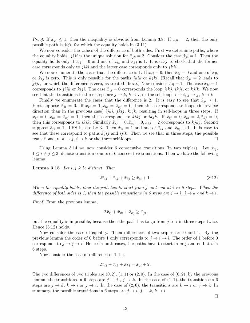
Proof. If xji ≤ 1, then the inequality is obvious from Lemma 3.8. If xji = 2, then the onlypossible path is jiji, for which the equality holds in (3.11).

We now consider the values of the difference of both sides. First we determine paths, wherethe equality holds. jiji is the unique solution for xjk = 2. Consider the case xji = 1. Then theequality holds only if xij = 0 and one of xik and xkj is 1. It is easy to check that the formercase corresponds only to jiki and the latter case corresponds only to jkji.

We now enumerate the cases that the difference is 1. If xji = 0, then xij = 0 and one of xikor xkj is zero. This is only possible for the paths jkik or kjki. (Recall that xji = 2 leads tojiji, for which the difference is zero, as treated above.) Now consider xji = 1. The case xij = 1corresponds to jijk or kiji. The case xij = 0 corresponds the loop jikj, ikji, or kjik. We nowsee that the transitions in three steps are j → k, k → i, or the self-loops i→ i, j → j, k → k.

Finally we enumerate the cases that the difference is 2. It is easy to see that xji ≤ 1.First suppose xji = 0. If xij = 1, xik = xkj = 0, then this corresponds to loops (in reversedirection than in the previous case) ijki, jkij, kijk, resulting in self-loops in three steps. Ifxij = 0, xik = xkj = 1, then this corresponds to kikj or ikjk. If xij = 0, xik = 2, xkj = 0,then this corresponds to ikik. Similarly xij = 0, xik = 0, xkj = 2 corresponds to kjkj. Secondsuppose xji = 1. LHS has to be 3. Then xij = 1 and one of xik and xkj is 1. It is easy tosee that these correspond to paths kjij and ijik. Then we see that in three steps, the possibletransitions are k → j, i→ k or the three self-loops.

Using Lemma 3.14 we now consider 6 consecutive transitions (in two triples). Let xij ,1 ≤ i 6= j ≤ 3, denote transition counts of 6 consecutive transitions. Then we have the followinglemma.

Lemma 3.15. Let i, j, k be distinct. Then

2xij + xik + xkj ≥ xji + 1. (3.12)

When the equality holds, then the path has to start from j and end at i in 6 steps. When thedifference of both sides is 1, then the possible transitions in 6 steps are j → i, j → k and k → i.

Proof. From the previous lemma,

2xij + xik + xkj ≥ xji

but the equality is impossible, because then the path has to go from j to i in three steps twice.Hence (3.12) holds.

Now consider the case of equality. Then differences of two triples are 0 and 1. By theprevious lemma the order of 0 before 1 only corresponds to j → i→ i. The order of 1 before 0corresponds to j → j → i. Hence in both cases, the paths have to start from j and end at i in6 steps.

Now consider the case of difference of 1, i.e.

2xij + xik + xkj = xji + 2.

The two differences of two triples are (0, 2), (1, 1) or (2, 0). In the case of (0, 2), by the previouslemma, the transitions in 6 steps are j → i , j → k. In the case of (1, 1), the transitions in 6steps are j → k, k → i or j → i. In the case of (2, 0), the transitions are k → i or j → i. Insummary, the possible transitions in 6 steps are j → i, j → k, k → i.

13

The final lemma is as follows.

Lemma 3.16. Consider a path of length T = 6k + 1, i.e., path with 6k steps. Then

2xij + xik + xkj ≥ xji + 2k − 1. (3.13)

If the equality holds, then the path has to be at i at time T .

Proof. We divide a path into k subpaths of length 6. Suppose that there exists a block for which

2xij + xik + xkj = xji + 1. (3.14)

In this block the path goes from j to i. Before another block of this type, the path has to comeback to j. But then there has to be some block of i→ k or i→ j. For these blocks

2xij + xik + xkj ≥ xji + 3. (3.15)

Therefore the deficit of 1 in (3.14) is compensated by the gain of 1 in (3.15). The lemma followsfrom this observation. The condition for equality also follows from this observation.

Now we will show a facet for the cases T = 6k and T = 6k + 3, k = 1, 2, . . . .

Proposition 3.17. For T = 6k + 3, the row vector

c = [5k + 2, 2k + 1,−4k − 1,−k,−k, 2k + 1]

defines a facet of P T modulo S3.

Proof. Consider

(5k + 2)x12 + (2k + 1)x13 + (2k + 1)x32 ≥ (4k + 1)x21 + kx23 + kx31. (3.16)

The RHS is written as

(3k + 1)x21 + k(x21 + x23 + x31) = (3k + 1)x21 + k(6k + 2− x12 − x13 − x32).

Hence (3.16) is equivalent to

(6k + 2)x12 + (3k + 1)x13 + (3k + 1)x32 ≥ (3k + 1)x21 + 2k(3k + 1).

Dividing by 3k + 1 > 0, this is equivalent to

2x12 + x13 + x32 ≥ x21 + 2k. (3.17)

A path has T − 1 = 6k + 2 steps. Consider the first 6k steps divided into triples of steps andapply Lemma 3.16 to the LHS. If the inequality in (3.13) is strict, then we only need to checkthat

2x12 + x13 + x32 ≥ x21for the remaining two steps. This is obvious, because a transition 21 has to be preceded orfollowed by some term on the left-hand side.

14

If equality holds in (3.13), at time 6k + 1, the path is at state 1 and then the penultimatestep is either 12 or 13. In either case we easily see that

2x12 + x13 + x32 > x21.

It remains to show that the first inequality for T = 6k + 3 defines a facet. Consider thefollowing 5 paths.

23132132132132 . . . 132132, 321321 . . . 321, 213232321321321 . . . 21,

213213213 . . . 213, 21321321321 . . . 3213212121.

The sufficient statistics for these paths are

[0, 2k, 2k, 1, 1, 2k], [0, 2k, 2k + 1, 0, 0, 2k + 1], [0, 2k − 1, 2k, 2, 0, 2k + 1]

[0, 2k + 1, 2k + 1, 0, 0, 2k], [2, 2k − 1, 2k + 2, 0, 0, 2k − 1].

This proves the proposition.

Now we consider T = 6k.

Proposition 3.18. For T = 6k, the row vector

c = [10k − 1, 4k,−8k + 2,−2k + 1,−2k + 1, 4k]

defines a facet of P T modulo S3.

Proof. Consider

(10k − 1)x12 + 4kx13 + 4kx32 ≥ (8k − 2)x21 + (2k − 1)x23 + (2k − 1)x31. (3.18)

The RHS is written as

(6k − 13)x21 + (2k − 1)(6k − 1− x12 − x13 − x32)

Hence (3.18) is equivalent to

(12k − 2)x12 + (6k − 1)x13 + (6k − 1)x32 ≥ (6k − 1)x21 + (2k − 1)(6k − 1)

or2x12 + x13 + x32 ≥ x21 + (2k − 1).

The rest of the proof is similar to that of Proposition 3.17.It remains to show that the first inequality for T = 6k defines a facet. Consider the following

5 paths.

232321321321 . . . 321, 213231321321 . . . 321, 321321321321 . . . 321,

213213 . . . 213, 212321321321 . . . 321.

The sufficient statistics for these paths are

[0, 2k − 2, 2k − 1, 2, 0, 2k], [0, 2k − 1, 2k − 1, 1, 1, 2k − 1], [0, 2k − 1, 2k, 0, 0, 2k]

[0, 2k, 2k, 0, 0, 2k − 1], [1, 2k − 2, 2k, 1, 0, 2k − 1].

15

Here we summarize all the inequalities in their original form and in their inhomogeneousform. Below we only present one of six of the inequalities with the understanding that for eachcase that any permutation of the labels {1, 2, 3} gives another facet. The inhomogeneous form isderived by substituting the equality n(T −1) = x12 +x13 +x21 +x23 +x31 +x32 into the originalform. Inhomogeneous form is essential for proving the normality of semigroup associated withthe design matrix AT .

For any T ≥ 5 homogeneous

c = [1, 0, 0, 0, 0, 0] · x ≥ 0

For any T ≥ 5, homogeneous

c = [T, T,−(T − 2), 1,−(T − 2), 1)] · x ≥ 0

inhomogeneousc = [1, 1,−1, 0,−1, 0] · x ≥ −n.

For any T odd, T ≥ 5, homogeneous

c = [1, 1,−1,−1, 1, 1] · x ≥ 0.

For any T ≥ 4 of the form T = 3k + 1, k ≥ 1, homogeneous

c = [2,−1,−1,−1, 2, 2] · x ≥ 0.

For any T ≥ 5 of the form T = 3k + 2, k ≥ 1, homogeneous

c = [2k + 1,−k,−k,−k, 2k + 1, 2k + 1] · x ≥ 0

inhomogeneous

x12 + x31 + x32 ≥ kn =T − 2

3n.

For any T ≥ 6, T :even, homogeneous

c = [3

2T − 1,

T

2,−T

2+ 1,−T

2+ 1,−T

2+ 1,

T

2] · x ≥ 0

inhomogeneous3x12 + x13 − x21 − x23 − x31 + x32 ≥ −n.

For T = 6k + 3, homogeneous

c = [5k + 2, 2k + 1,−4k − 1,−k,−k, 2k + 1] · x ≥ 0

inhomogeneous

2x12 + x13 − x21 + x32 ≥T − 3

3n.

For T = 6k, homogeneous

c = [10k − 1, 4k,−8k + 2,−2k + 1,−2k + 1, 4k] · x ≥ 0

inhomogeneous

2x12 + x13 − x21 + x32 ≥T − 3

3n.

16

3.3. There are only 24 facets

In the previous section, we give 24 facets of the polytope P T for every T ≥ 3, where death ofthe 24 facets depend on T mod 6. Here, we discuss how these 24 facets are enough to describethe polytope P T (the convex hull of the columns of AT ), depending on T . Let CT := cone(AT ).

Recall that the columns of AT are on the following hyperplane

HT = {(x12, . . . , x32) | T − 1 = x12 + · · ·+ x32}.

Then it is clear by Proposition 3.4 that

P T = CT ∩HT .

Let FT denote the set of facets of the pointed cone CT . Then the facets F of P T (within HT )are of the form F ⊆ HT , F ⊆ FT .

For every T , let FT denote the 24 facets prescribed in the previous section, and let FT denotethe set of all facets of P 3,T . Therefore we have a certain subset FT ⊂ FT and we need to showthat FT = FT . Let CT denote the polyhedral cone defined by FT . It follows that CT ⊃ CT . Notethat FT = FT if and only if CT = CT . Also let

PT = CT ∩HT .

Then PT ⊃ P T and PT = P T if and only if CT = CT .The above argument shows that to prove FT = FT it suffices to show that

PT ⊂ P T . (3.19)

Let VT be the set of vertices of PT . Then in order to show (3.19), it suffices to show that

VT ⊂ P T .

Hence, if we can obtain explicit expressions of the vertices of VT and can show that each vertexbelongs to P T , we are done.

In the previous section, we used only the condition T − 1 = x12 + · · · + x32 to settle theequivalence between the homogeneous and inhomogeneous inequalities defining the 24 the facetsof P T . Hence the homogeneous and the inhomogeneous inequalities are equivalent on HT .Therefore, for each r = 0, . . . , 5, there exists a polyhedral region defined by 24 fixed affinehalf-spaces, say Qr, such that

PT = Qr ∩HT , T = 6k + r, k = 1, 2, . . .

Since Qr is a polyhedral region it can be written as a Minkowski sum of a polytope P r anda cone Cr:

Qr = P r + Cr.

Please note that r is modulo 6, but T is not. Recall the Minkowski sum of two sets A,B ⊆ Rnis simply { a + b | a ∈ A, b ∈ B }. The six cones and polytopes defining Qr for r = 0, . . . , 5are given in the Appendix and were computed using Polymake [3]. For each vertex v of P r andeach extreme ray e of Cr let lv,e denote the half-line emanating from v in the direction e:

lv,e = {v + te | t ≥ 0}

17

Given the explicit expressions of v and e we can solve

[1, 1, 1, 1, 1, 1] · (v + te) = T − 1

for t and get

t := t(T,v, e) =T − 1− [1, . . . , 1]v

(1, . . . , 1)e.

Then v + t(T,v, e)e ∈ HT . Note that

VT ⊂ {v + t(T,v, e)e | v : vertex of P r, e : extreme ray of Cr}.

Also clearly

{v + t(T,v, e)e | v : vertex of P r, e : extreme ray of Cr} ∈ PT = conv(VT ).

The above argument shows that for proving FT = FT it suffices to show that

{v + t(T,v, e)e | v : vertex of P r, e : extreme ray of Cr} ∈ P T . (3.20)

For proving (3.20) the following lemma is useful.

Lemma 3.19. Let v ∈ P r and e ∈ C. If v + t(T,v, e)e ∈ P T ∩ Z6 for some T , then v + t(T +6k,v, e)e ∈ P T+6k for all k ≥ 0.

Proof. If x := v+ t(T,v, e)e ∈ P T ∩Z6 for some T then x corresponds to a path of length T onthree states with no loops (word in 〈3〉T ). Suppose e is a two-loop (three-loop) e.g. 121 (1231).Then x + (3k)e ∈ P T+6k (x + (2k)e ∈ P T+6k). That is, since x is an integer point (a path)contained in P T , we can simply add three (or two depending on the loop) copies of the loop eand we will be guaranteed to have a path of the correct length meaning it will be contained inP T+6.

By this lemma we need to compute Cr only for some special small T ’s. We computedall vertices and all rays for the cases T = 12, 7, 20, 9, 16, 11. The software to generate thedesign matrices can be found at https://github.com/dchaws/GenWordsTrans and the designmatrices and some other material can be found at http://www.davidhaws.net/THMC.html. Byour computational result and Lemma 3.19 we verified the following proposition.

Proposition 3.20. The rays of the cones Cr for r = 0, . . . , 5 are ((1,0,1,0,0,0), (1,0,0,1,1,0),(0,1,1,0,0,1), (0,1,0,0,1,0), (0,0,0,1,0,1)). In terms of the state graph, the rays correspond tothe five loops 121, 131, 232, 1231, and 1321.

Note that Cr, r = 0, . . . , 5 are common and we denote them as C hereafter. Also note thatthe rays of the cone Cr are very simple. Proposition 3.20 implies the following theorem.

Theorem 3.21. The 24 facets given in Propositions 3.6, 3.7, 3.9, 3.10, 3.12, 3.17, 3.18 (de-pending on T mod 6) are all the facets of P T = conv(AT ).

18

4. Normality of the semigroup

From the definition of normality of a semigroup defined in Section 2.3, the semigroup NATdefined by the design matrix is normal if it coincides with the elements in both, the integerlattice ZAT and the cone cone(AT ).

In this section, we provide an inductive prove on the normality of the semigroup NAT forarbitrary T . For the first 135 values of T , we computationally verified the normality. Thesecases served as an inductive base for a proof of normality for a general T .

Lemma 4.1. The semigroup NAT is normal for 1 ≤ T ≤ 135.

Proof. The normality of the design matrices AT for 1 ≤ T ≤ 135 was confirmed computationallyusing the software Normaliz [1]. The software to generate the design matrices and the scriptsto run the computations are available at https://github.com/dchaws/GenWordsTrans.

Using Lemma 4.1, we have prove normality in the general case in what follows.

Theorem 4.2. The semigroup NAT is normal for any T ∈ N.

Proof. We need to show that given any transition counts x12, . . . , x32, such that their sum isdivisible by T − 1 and the counts lie in cone(AT ), there exists a set of paths having thesetransition counts. Write x = [x12, x13, x21, x23, x31, x32]

T and 16 = [1, 1, 1, 1, 1, 1]. Let

n = 16 · x/(T − 1)

denote the number of the paths. Note that n is determined from T and x.We listed above inhomogeneous forms of inequalities defining facets. In all cases T = 6k+ r,

r = 0, 1, . . . , 5, the inhomogeneous form of inequalities for n paths can be put in the form

c12x12 + · · ·+ c32x32 ≥ aTn, (4.1)

where c12, . . . , c32, aT do not depend on n.Let Qr denote the polyhedral region defined by the inequalities for T = 6k + r and just one

path. We have computed the V -representation

Qr = P r + C,

where P r is a polytope and C is the common cone. The n-th dilation of Qr is

Qrn := nQr = nP r + nC = nP r + C.

Then from (4.1) we have

cone(AT ) ∩ {x | 16 · x = n(T − 1)} = Qrn ∩ {x | 16 · x = n(T − 1)}.

We now look at vertices of P r from Appendix. The vertex [0,3,4,3,0,7] for Q2 has the largestL1-norm, which is 17. Hence the sum of elements of these vertices P rn are at most 17n.

Any non-negative integer vector x with 16 ·x = n(T −1), T = 6k+ r, belonging to cone(AT )is written as

x = b + α1e1 + α2e2 + α3e3 + α4e4 + α5e5, b ∈ nP r1 , αi ≥ 0, i = 1, . . . , 5.

19

Taking the inner product with 16 (i.e. the L1-norm) we have

16 · b ≤ 17n. (4.2)

Hencen(T − 1) = 16 · x ≤ 17n+ 2(α1 + α2 + α3) + 3(α4 + α5).

Consider the case thatα1, α2, α3 ≤ 3n, α4, α5 ≤ 2n. (4.3)

Thenn(T − 1) = 16 · x ≤ 17n+ 18n+ 12n = 47n

or T ≤ 48. Hence if T > 48 we have at least one of

α1 > 3n, α2 > 3n, α3 > 3n, α4 > 2n, α5 > 2n. (4.4)

Now we employ induction on k for T = 6k + r. Note that we arbitrarily fix n ≥ 1 and useinduction on k. For k ≤ 21 we have T = 6k + r ≤ 126 + r ≤ 131 < 135 and the normality holdsby the computational results.

Now consider k > 22 and let T = 6k + r. In this case at least one inequality of (4.4) holds.Let

x ∈ cone(AT ) ∩ {x | 16 · x = n(T − 1)}First consider x such that α1 > 3n. (The argument for α2 and α3 is the same.) Let

x = x− 3ne1 ∈ cone(AT ) ∩ {x | 16 · x = n(T − 1− 6)}

Our inductive assumption is that there exists a set of paths w1, . . . ,wn of length T − 6 havingx as the transition counts. We now form n partial paths of length 6:

n times ijijij

Note that instead of ijijij we can also use jijiji. We now argue that these n partial paths canbe appended (at the end or at the beginning) of each path w1, . . . ,wn.

Let w1 = s1 . . . sT−6. If s1 6= sT−6, then

{s1, sT−6} ∩ {i, j} 6= ∅,

since |S| = 3. In this case we see that at least one of the following 4 operations is possible

1. put ijijij at the end of w1

2. put jijiji at the end of w1

3. put ijijij in front of w1

4. put jijiji in front of w1

Hence w1 can be extended to a path of length T . Now consider the case that s1 = sT−6,i.e., w1 is a cycle. It may happen that s1 6= i, j. But a cycle can be rotated, i.e., instead ofw1 = s1 . . . sT−6 we can take

w′1 = s2s3 . . . sT−6s1

where s2 6= s1, hence s2 = i or j. Then either ijijij or jijiji can be put in front of w′1 and w′1can be extended. Therefore we see that w1 can be extended in any case. Similarly w2, . . . ,wn

can be extended.The case of α4 > 2n is trivial. The path ijkijk can be rotated as jkijki or kijkij. Therefore

one of them can be appended to each of w1, . . . ,wn.

20

5. Discussion

In this paper, we considered only the situation of the toric homogeneous Markov chain(THMC) model (1.1) for S = 3, with the extra assumption of having non-zero transition proba-bilities only when the transition is between two different states. In this setting, we described thehyperplane representations of the design polytope for any T ≥ 4, and from this representationwe showed that the semigroup generated by the columns of the design matrix AT is normal.

We recall from Lemma 4.14 in [10], that a given set of integer vectors {a1, . . . ,an} is a gradedset, if there exists w ∈ QS2

such that ai ·w = 1. In our setting, the set of columns of the designmatrix AT is a graded set, as each of its columns add up to T −1, so we let w = ( 1

T−1 , . . . ,1

T−1).In his same book, Sturmfels provided a way to bound the generators of the toric ideal

associated to an integer matrix A, the precise statement is the following.

Theorem 5.1 (Theorem 13.14 in[10]). Let A ⊂ Zd be a graded set such that the semigroupgenerated by the elements in A is normal. Then the toric ideal IA associate with the set A isgenerated by homogeneous binomials of degree at most d.

In our setting, Theorem 4.2 demonstrates the normality of the semigroup generated by thecolumns of the design matrix AT , so as a consequence we obtain the following theorem:

Theorem 5.2. For S = 3 and for any T ≥ 4, a Markov basis for the toric ideal IAT associatedto the THMC model (without loops and initial parameters) consists of binomials of degree atmost 6.

The bound provided by Theorem 5.2 seems not to be sharp, in the sense that there existsMarkov basis whose elements have degree strictly less than 6. In our computational experiments,we found evidence that more should be true. Our observations hold in a more general setting.For any S and T , let AS,T denote the design matrix for the THMC model in S states.

Conjecture 5.3. Fix S ≥ 3; then, for every T ≥ 4, there is a Markov basis for the toric idealIAS,T consisting of binomials of degree at most S − 1, and there is a Grobner basis with respectto some term ordering consisting of binomials of degree at most S.

We also noted that for S ≥ 4, the semigroup generated by the columns of AS,T is not normal.For example, S = 4, T = 8, 1

2a4,412121212 + 1

2a4,434343434 is an integral solution in the intersection

between the cone and the integer lattice. However this does not form a path. Thus it isinteresting to investigate that for any S ≥ 4 and for any T ≥ 5 what the necessary and sufficientcondition is for the semigroup generated by the columns of the design matrix AS,T to be normal.

6. appendix

Cr = C := cone(

[1, 0, 1, 0, 0, 0], [1, 0, 0, 1, 1, 0], [0, 1, 1, 0, 0, 1], [0, 1, 0, 0, 1, 0], [0, 0, 0, 1, 0, 1]).

for r = 0, . . . , 5.vert(Q0) := ([3, 0, 0, 4, 4, 0], [4, 0, 0, 3, 4, 0], [2, 0, 0, 4, 3, 2], [2, 2, 0, 2, 5, 0], [4, 0, 2, 2, 3, 0], [0, 4, 3, 0, 0, 4], [0, 2, 2, 2, 0, 5], [0, 4,

2, 0, 2, 3], [2, 2, 4, 0, 0, 3], [3, 0, 0, 4, 2, 2], [3, 2, 0, 2, 4, 0], [5, 0, 2, 2, 2, 0], [0, 2, 2, 1, 0, 2], [1, 2, 2, 0, 0, 2], [0, 1, 1, 0, 0, 1], [1, 0, 0, 1,1, 0], [2, 1, 0, 2, 2, 0], [2, 0, 0, 2, 2, 1], [0, 2, 2, 0, 1, 2], [2, 0, 1, 2, 2, 0], [2, 3, 4, 0, 0, 2], [0, 5, 2, 0, 2, 2], [0, 3, 2, 2, 0, 4], [4, 0, 2, 3, 2, 0],[2, 2, 0, 3, 4, 0], [2, 0, 0, 5, 2, 2], [4, 0, 0, 4, 3, 0], [2, 2, 5, 0, 0, 2], [0, 4, 3, 0, 2, 2], [0, 2, 3, 2, 0, 4], [0, 4, 4, 0, 0, 3], [0, 3, 4, 0, 0, 4], [2, 0,2/3, 2, 7/3, 0], [4/3, 2/3, 2/3, 4/3, 7/3, 2/3], [8/5, 2/5, 4/5, 6/5, 11/5, 0], [2, 0, 0, 2, 7/3, 2/3], [6/5, 2/5, 0, 8/5, 11/5, 4/5], [3/2, 0, 0, 3/2,2, 0], [2/3, 4/3, 4/3, 2/3, 2/3, 7/3], [0, 8/5, 6/5, 2/5, 4/5, 11/5], [0, 2, 2, 0, 2/3, 7/3], [2/3, 2, 2, 0, 0, 7/3], [4/5, 6/5, 8/5, 2/5, 0, 11/5], [0,3/2, 3/2, 0, 0, 2], [7/3, 2/3, 2/3, 4/3, 4/3, 2/3], [11/5, 0, 2/5, 8/5, 6/5, 4/5], [7/3, 0, 0, 2, 2, 2/3], [7/3, 2/3, 0, 2, 2, 0], [11/5, 4/5, 2/5, 6/5,8/5, 0], [2, 0, 0, 3/2, 3/2, 0], [1/2, 1, 2, 1, 0, 3/2], [3/2, 0, 1, 2, 1, 1/2], [1, 1, 3/2, 1/2, 0, 2], [2, 0, 1/2, 3/2, 1, 1], [2, 1, 1/2, 1, 3/2, 0], [1, 2,3/2, 0, 1/2, 1], [0, 2, 1, 1, 1/2, 3/2], [1, 1, 0, 2, 3/2, 1/2], [0, 3/2, 1, 1/2, 1, 2], [1, 1/2, 0, 3/2, 2, 1], [1/2, 3/2, 2, 0, 1, 1], [3/2, 1/2, 1, 1, 2, 0],[0, 2, 3/2, 0, 0, 3/2], [2/3, 7/3, 2, 0, 0, 2], [4/5, 11/5, 8/5, 0, 2/5, 6/5], [0, 7/3, 2, 2/3, 0, 2], [0, 11/5, 6/5, 4/5, 2/5, 8/5], [2/3, 7/3, 4/3, 2/3,2/3, 4/3], [3/2, 0, 0, 2, 3/2, 0], [6/5, 4/5, 0, 11/5, 8/5, 2/5], [2, 2/3, 0, 7/3, 2, 0], [2, 0, 2/3, 7/3, 2, 0], [8/5, 0, 4/5, 11/5, 6/5, 2/5], [4/3, 2/3,2/3, 7/3, 4/3, 2/3], [0, 3/2, 2, 0, 0, 3/2], [2/5, 6/5, 11/5, 4/5, 0, 8/5], [0, 2, 7/3, 2/3, 0, 2], [2/5, 8/5, 11/5, 0, 4/5, 6/5], [0, 2, 7/3, 0, 2/3, 2],[2/3, 4/3, 7/3, 2/3, 2/3, 4/3] ).

21

vert[Q1] := [([2, 0, 1, 2, 1, 0], [1, 0, 0, 3, 1, 1], [1, 1, 0, 2, 2, 0], [2, 1, 3, 0, 0, 0], [0, 3, 1, 0, 2, 0], [0, 1, 1, 2, 0, 2], [3, 0, 1, 1, 1, 0], [2, 0,0, 2, 1, 1], [2, 1, 2, 0, 0, 1], [2, 1, 0, 1, 2, 0], [0, 1, 0, 2, 0, 3], [0, 3, 0, 0, 2, 1], [0, 0, 0, 0, 0, 0], [0, 3, 1, 0, 1, 1], [0, 2, 1, 1, 0, 2], [1, 2, 2, 0, 0,1], [1, 2, 0, 1, 2, 0], [1, 0, 0, 3, 0, 2], [3, 0, 2, 1, 0, 0], [3, 0, 2, 0, 1, 0], [1, 0, 0, 2, 1, 2], [1, 2, 0, 0, 3, 0], [1, 1, 2, 0, 0, 2], [0, 1, 1, 1, 0, 3], [0, 2,1, 0, 1, 2], [2, 0, 1, 1, 2, 0], [1, 0, 0, 2, 2, 1], [1, 1, 0, 1, 3, 0], [2, 0, 3, 0, 0, 1], [0, 0, 1, 2, 0, 3], [0, 2, 1, 0, 2, 1], [1, 1, 3, 0, 0, 1], [0, 2, 2, 0, 1,1], [0, 1, 2, 1, 0, 2], [0, 2, 0, 1, 3, 0], [0, 0, 0, 3, 1, 2], [2, 0, 2, 1, 1, 0], [1/2, 1/2, 1/2, 1, 1/2, 0], [0, 1/2, 1/2, 1, 1/2, 1/2], [0, 1, 1/2, 1/2, 1, 0],[1/2, 1/2, 1, 1/2, 1/2, 0], [1, 1/2, 0, 1/2, 1/2, 1/2], [1/2, 1, 0, 0, 1, 1/2], [1/2, 1/2, 0, 1/2, 1/2, 1], [1, 1/2, 1/2, 0, 1/2, 1/2], [1/2, 1/2, 0, 1, 0,1], [1/2, 1, 0, 1/2, 1/2, 1/2], [1, 1/2, 1/2, 1/2, 0, 1/2], [1/2, 1, 1/2, 1/2, 1/2, 0], [1/2, 1/2, 1/2, 1, 0, 1/2], [1, 1/2, 1, 1/2, 0, 0], [1/2, 1, 1/2,1/2, 0, 1/2], [1/2, 1/2, 1/2, 0, 1, 1/2], [1/2, 0, 1/2, 1/2, 1/2, 1], [1, 0, 1, 0, 1/2, 1/2], [1/2, 1/2, 1/2, 0, 1/2, 1], [0, 1/2, 1/2, 1/2, 1, 1/2], [0,0, 1/2, 1, 1/2, 1], [1/2, 0, 1, 1/2, 1/2, 1/2], [1/2, 0, 1/2, 1/2, 1, 1/2], [0, 1/2, 1, 1/2, 1/2, 1/2] ).

vert[Q2] :=([2, 2, 0, 3, 4, 0], [4, 0, 2, 3, 2, 0], [2, 0, 0, 5, 2, 2], [0, 2, 2, 3, 0, 4], [0, 7, 4, 0, 3, 3], [0, 4, 2, 1, 2, 2], [3, 4, 7, 0, 0, 3], [2, 2, 4,1, 0, 2], [3, 0, 0, 4, 2, 2], [5, 0, 2, 2, 2, 0], [3, 2, 0, 2, 4, 0], [3, 2, 4, 0, 0, 2], [0, 7, 3, 0, 3, 4], [1, 4, 2, 0, 2, 2], [0, 4, 3, 3, 0, 7], [1, 2, 2, 2, 0, 4],[0, 2, 1, 0, 1, 1], [0, 1, 1, 1, 0, 2], [1, 1, 0, 1, 2, 0], [1, 1, 2, 0, 0, 1], [2, 0, 1, 1, 1, 0], [1, 0, 0, 2, 1, 1], [2, 1, 0, 4, 2, 2], [4, 1, 2, 2, 2, 0], [7, 0, 3,4, 3, 0], [4, 0, 0, 7, 3, 3], [0, 5, 2, 0, 2, 2], [0, 3, 2, 2, 0, 4], [2, 3, 0, 2, 4, 0], [2, 3, 4, 0, 0, 2], [2, 2, 0, 2, 4, 1], [4, 3, 0, 3, 7, 0], [4, 0, 2, 2, 2,1], [7, 0, 3, 3, 4, 0], [0, 4, 2, 0, 2, 3], [0, 2, 2, 2, 0, 5], [2, 0, 0, 4, 2, 3], [2, 2, 4, 0, 0, 3], [2, 2, 4, 0, 1, 2], [0, 3, 4, 3, 0, 7], [0, 2, 2, 2, 1, 4], [3,3, 7, 0, 0, 4], [3, 3, 0, 4, 7, 0], [3, 0, 0, 7, 4, 3], [2, 0, 1, 4, 2, 2], [2, 2, 1, 2, 4, 0], [2, 2, 0, 2, 5, 0], [4, 0, 2, 2, 3, 0], [2, 0, 0, 4, 3, 2], [0, 4, 2,0, 3, 2], [0, 4, 3, 0, 2, 2], [0, 2, 3, 2, 0, 4], [4, 0, 3, 2, 2, 0], [2, 2, 5, 0, 0, 2], [4/3, 2/3, 2/3, 7/3, 4/3, 2/3], [2/3, 4/3, 4/3, 5/3, 2/3, 4/3], [7/6,1/3, 4/3, 5/3, 2/3, 5/6], [5/6, 2/3, 5/3, 4/3, 1/3, 7/6], [1/2, 1, 2, 2, 0, 5/2], [3/2, 1, 3, 1, 0, 3/2], [5/2, 0, 2, 2, 1, 1/2], [3/2, 0, 1, 3, 1, 3/2],[7/3, 2/3, 2/3, 4/3, 4/3, 2/3], [5/3, 4/3, 4/3, 2/3, 2/3, 4/3], [4/3, 2/3, 7/6, 5/6, 1/3, 5/3], [5/3, 1/3, 5/6, 7/6, 2/3, 4/3], [1, 1, 3/2, 3/2, 0, 3],[2, 1, 5/2, 1/2, 0, 2], [3, 0, 3/2, 3/2, 1, 1], [2, 0, 1/2, 5/2, 1, 2], [1/3, 2/3, 2/3, 1/3, 1/3, 2/3], [2/3, 1/3, 1/3, 2/3, 2/3, 1/3], [5/3, 4/3, 5/6,2/3, 7/6, 1/3], [4/3, 5/3, 7/6, 1/3, 5/6, 2/3], [3, 1, 3/2, 1, 3/2, 0], [2, 2, 1/2, 1, 5/2, 0], [1, 3, 3/2, 0, 3/2, 1], [2, 2, 5/2, 0, 1/2, 1], [0, 3, 1, 1,3/2, 3/2], [0, 2, 1, 2, 1/2, 5/2], [1, 2, 0, 2, 5/2, 1/2], [1, 1, 0, 3, 3/2, 3/2], [1/3, 5/3, 2/3, 4/3, 5/6, 7/6], [2/3, 4/3, 1/3, 5/3, 7/6, 5/6], [4/3,5/3, 2/3, 4/3, 4/3, 2/3], [2/3, 7/3, 4/3, 2/3, 2/3, 4/3], [0, 5/2, 1, 1/2, 2, 2], [0, 3/2, 1, 3/2, 1, 3], [1, 3/2, 0, 3/2, 3, 1], [1, 1/2, 0, 5/2, 2, 2],[1/3, 7/6, 2/3, 5/6, 4/3, 5/3], [2/3, 5/6, 1/3, 7/6, 5/3, 4/3], [4/3, 2/3, 2/3, 4/3, 4/3, 5/3], [2/3, 4/3, 4/3, 2/3, 2/3, 7/3], [3/2, 3/2, 3, 0, 1, 1],[1/2, 5/2, 2, 0, 2, 1], [3/2, 3/2, 1, 1, 3, 0], [5/2, 1/2, 2, 1, 2, 0], [5/6, 7/6, 5/3, 1/3, 4/3, 2/3], [7/6, 5/6, 4/3, 2/3, 5/3, 1/3], [2/3, 4/3, 4/3,2/3, 5/3, 4/3], [4/3, 2/3, 5/3, 4/3, 4/3, 2/3], [4/3, 2/3, 2/3, 4/3, 7/3, 2/3], [2/3, 4/3, 7/3, 2/3, 2/3, 4/3] ).

vert[Q3] := ([1, 0, 0, 0, 1, 0], [1, 2, 0, 1, 4, 0], [1, 0, 0, 3, 2, 2], [3, 0, 2, 1, 2, 0], [0, 1, 0, 0, 0, 1], [0, 3, 1, 0, 2, 2], [0, 1, 1, 2, 0, 4], [2, 1,3, 0, 0, 2], [2, 2, 0, 1, 3, 0], [2, 0, 0, 3, 1, 2], [4, 0, 2, 1, 1, 0], [0, 0, 0, 0, 0, 0], [2, 2, 3, 0, 0, 1], [0, 2, 1, 2, 0, 3], [0, 4, 1, 0, 2, 1], [3, 0, 2, 2, 1,0], [1, 0, 0, 4, 1, 2], [1, 2, 0, 2, 3, 0], [1, 0, 0, 1, 0, 0], [2, 1, 4, 0, 0, 1], [0, 1, 2, 2, 0, 3], [0, 3, 2, 0, 2, 1], [0, 1, 1, 0, 0, 0], [0, 0, 1, 0, 0, 1], [0, 0,0, 1, 1, 0]).

vert[Q4] := ([0, 2, 2, 2, 0, 3], [3, 0, 1, 3, 2, 0], [2, 1, 0, 3, 3, 0], [2, 0, 0, 4, 2, 1], [0, 6, 4, 0, 2, 3], [0, 3, 2, 1, 1, 2], [2, 4, 6, 0, 0, 3], [1, 2,3, 1, 0, 2], [3, 0, 0, 3, 2, 1], [4, 0, 1, 2, 2, 0], [3, 1, 0, 2, 3, 0], [2, 2, 3, 0, 0, 2], [0, 4, 3, 2, 0, 6], [0, 6, 3, 0, 2, 4], [1, 3, 2, 0, 1, 2], [1, 2, 2, 1, 0,3], [0, 1, 1, 0, 0, 1], [1, 0, 0, 1, 1, 0], [2, 1, 0, 3, 2, 1], [3, 1, 1, 2, 2, 0], [6, 0, 2, 4, 3, 0], [4, 0, 0, 6, 3, 2], [0, 4, 2, 0, 1, 2], [0, 3, 2, 1, 0, 3], [1, 3,3, 0, 0, 2], [2, 2, 0, 2, 3, 0], [2, 1, 0, 2, 3, 1], [4, 2, 0, 3, 6, 0], [3, 0, 1, 2, 2, 1], [6, 0, 2, 3, 4, 0], [0, 2, 2, 1, 0, 4], [0, 3, 2, 0, 1, 3], [1, 2, 3, 0, 0,3], [2, 0, 0, 3, 2, 2], [1, 2, 3, 0, 1, 2], [0, 3, 4, 2, 0, 6], [0, 2, 2, 1, 1, 3], [2, 3, 6, 0, 0, 4], [3, 2, 0, 4, 6, 0], [3, 0, 0, 6, 4, 2], [2, 0, 1, 3, 2, 1], [2, 1,1, 2, 3, 0], [2, 1, 0, 2, 4, 0], [2, 0, 0, 3, 3, 1], [3, 0, 1, 2, 3, 0], [0, 3, 2, 0, 2, 2], [0, 2, 3, 1, 0, 3], [0, 3, 3, 0, 1, 2], [1, 2, 4, 0, 0, 2], [3, 0, 2, 2, 2,0], [5/3, 1/3, 1/3, 8/3, 5/3, 1/3], [1/3, 5/3, 5/3, 4/3, 1/3, 5/3], [1/2, 1, 2, 1, 0, 3/2], [3/2, 0, 1, 2, 1, 1/2], [8/3, 1/3, 1/3, 5/3, 5/3, 1/3], [4/3,5/3, 5/3, 1/3, 1/3, 5/3], [1, 1, 3/2, 1/2, 0, 2], [2, 0, 1/2, 3/2, 1, 1], [2, 1, 1/2, 1, 3/2, 0], [1, 2, 3/2, 0, 1/2, 1], [0, 2, 1, 1, 1/2, 3/2], [1, 1, 0,2, 3/2, 1/2], [5/3, 4/3, 1/3, 5/3, 5/3, 1/3], [1/3, 8/3, 5/3, 1/3, 1/3, 5/3], [0, 3/2, 1, 1/2, 1, 2], [1, 1/2, 0, 3/2, 2, 1], [5/3, 1/3, 1/3, 5/3, 5/3,4/3], [1/3, 5/3, 5/3, 1/3, 1/3, 8/3], [1/2, 3/2, 2, 0, 1, 1], [3/2, 1/2, 1, 1, 2, 0], [1/3, 5/3, 5/3, 1/3, 4/3, 5/3], [5/3, 1/3, 4/3, 5/3, 5/3, 1/3],[5/3, 1/3, 1/3, 5/3, 8/3, 1/3], [1/3, 5/3, 8/3, 1/3, 1/3, 5/3]).

vert[Q5] := ([1, 2, 0, 2, 3, 0], [3, 0, 2, 2, 1, 0], [1, 0, 0, 4, 1, 2], [0, 1, 1, 3, 0, 3], [0, 4, 1, 0, 3, 0], [3, 1, 4, 0, 0, 0], [0, 4, 0, 0, 3, 1], [0, 1,0, 3, 0, 4], [4, 0, 2, 1, 1, 0], [2, 0, 0, 3, 1, 2], [3, 1, 3, 0, 0, 1], [2, 2, 0, 1, 3, 0], [0, 1, 0, 0, 1, 0], [0, 0, 0, 1, 0, 1], [1, 0, 1, 0, 0, 0], [1, 0, 0, 4, 0,3], [4, 0, 3, 1, 0, 0], [0, 2, 1, 2, 0, 3], [0, 4, 1, 0, 2, 1], [1, 3, 0, 1, 3, 0], [2, 2, 3, 0, 0, 1], [1, 3, 0, 0, 4, 0], [1, 0, 0, 3, 1, 3], [0, 3, 1, 0, 2, 2], [0, 1,1, 2, 0, 4], [4, 0, 3, 0, 1, 0], [2, 1, 3, 0, 0, 2], [3, 0, 2, 1, 2, 0], [1, 0, 0, 3, 2, 2], [1, 2, 0, 1, 4, 0], [0, 3, 1, 0, 3, 1], [0, 0, 1, 3, 0, 4], [3, 0, 4, 0, 0,1], [3, 0, 3, 1, 1, 0], [0, 0, 0, 4, 1, 3], [0, 3, 0, 1, 4, 0], [2, 1, 4, 0, 0, 1], [0, 3, 2, 0, 2, 1], [0, 1, 2, 2, 0, 3], [1/2, 1/2, 1/2, 2, 1/2, 1], [3/2, 1/2,3/2, 1, 1/2, 0], [1/2, 3/2, 1/2, 1, 3/2, 0], [0, 1/2, 1/2, 2, 1/2, 3/2], [0, 2, 1/2, 1/2, 2, 0], [3/2, 1/2, 2, 1/2, 1/2, 0], [1, 1/2, 0, 3/2, 1/2, 3/2],[1, 3/2, 0, 1/2, 3/2, 1/2], [2, 1/2, 1, 1/2, 1/2, 1/2], [2, 1/2, 3/2, 0, 1/2, 1/2], [1/2, 1/2, 0, 3/2, 1/2, 2], [1/2, 2, 0, 0, 2, 1/2], [2, 1/2, 3/2, 1/2,0, 1/2], [1/2, 2, 0, 1/2, 3/2, 1/2], [1/2, 1/2, 0, 2, 0, 2], [1/2, 1/2, 1/2, 2, 0, 3/2], [2, 1/2, 2, 1/2, 0, 0], [1/2, 2, 1/2, 1/2, 3/2, 0], [1/2, 1, 1/2,3/2, 0, 3/2], [1/2, 2, 1/2, 1/2, 1, 1/2], [3/2, 1, 3/2, 1/2, 0, 1/2], [1/2, 3/2, 1/2, 0, 2, 1/2], [1/2, 0, 1/2, 3/2, 1/2, 2], [2, 0, 2, 0, 1/2, 1/2], [3/2,1/2, 3/2, 0, 1/2, 1], [1/2, 1/2, 1/2, 1, 1/2, 2], [1/2, 3/2, 1/2, 0, 3/2, 1], [3/2, 0, 2, 1/2, 1/2, 1/2], [0, 0, 1/2, 2, 1/2, 2], [0, 3/2, 1/2, 1/2, 2,1/2], [1/2, 1, 1/2, 1/2, 2, 1/2], [1/2, 0, 1/2, 3/2, 1, 3/2], [3/2, 0, 3/2, 1/2, 1, 1/2], [0, 1/2, 1, 3/2, 1/2, 3/2], [0, 3/2, 1, 1/2, 3/2, 1/2], [1, 1/2,2, 1/2, 1/2, 1/2]).

[1] Bruns, W., Ichim, B., Soger, C., 2011. Normaliz, a tool for computations in affine monoids,vector configurations, lattice polytopes, and rational cones.

[2] Diaconis, P., Sturmfels, B., 1998. Algebraic algorithms for sampling from conditional dis-tributions. The Annals of Statistics 26 (1), 363–397.

[3] Gawrilow, E., Joswig, M., 2000. polymake: a framework for analyzing convex polytopes. In:Kalai, G., Ziegler, G. M. (Eds.), Polytopes — Combinatorics and Computation. Birkhauser,pp. 43–74.

[4] Hara, H., Takemura, A., 2011. A markov basis for two-state toric homogeneous markovchain model without initial paramaters. Journal of Japan Statistical Society 41, 33–49.

[5] Haws, D., Martin del Campo, A., Yoshida, R., 2011. Degree bounds for a minimal markovbasis for the three-state toric homogeneous markov chain model. Proceedings of the Sec-ond CREST–SBM International Conference, “Harmony of Grobner Bases and the ModernIndustrial Society”.

[6] Miller, E., Sturmfels, B., 2005. Combinatorial commutative algebra. Graduate texts inmathematics. Springer.URL http://books.google.com/books?id=CqEHpxbKgv8C

22

[7] Pachter, L., Sturmfels, B., 2005. Algebraic Statistics for Computational Biology. CambridgeUniversity Press, Cambridge, UK.

[8] Pardoux, E., 2009. Markov Processes and Applications: Algorithms, Networks, Genome andFinance. Wiley Series in Probability and Statistics Series. Wiley, John & Sons, Incorporated.

[9] Schrijver, A., 1986. Theory of Linear and Integer Programming. John Wiley & Sons, Inc.,New York, NY, USA.

[10] Sturmfels, B., 1996. Grobner Bases and Convex Polytopes. Vol. 8 of University LectureSeries. American Mathematical Society, Providence, RI.

[11] Takemura, A., Hara, H., 2012. Markov chain monte carlo test of toric homogeneous markovchains. Statistical Methodology. doi:10.1016/j.stamet.2011.10.004. 9, 392–406.

[12] Yap, C.-K., 2000. Fundamental problems of algorithmic algebra. Oxford University Press.URL http://books.google.com/books?id=YzjvQ-TSQ4gC

23