A Sequential Markov Chain Monte Carlo Approach to Set-up Adjustment of a Process over a Set of Lots

Journal of Applied Statistics, VS RoutledgeVol. 31, No. 5, 499-520, June 2004 1^

A Sequential Markov Chain MonteCarlo Approach to Set-up Adjustmentof a Process over a Set of Lots

B. M. COLOSIMO*, R. PAN** AND E. DEL CASTILLO!*Dipariimenia di Meccanica - Poliieaiica di Mllano, 20133 Milano, Ualy. **Deparlmeni ofMechanical & Industrial Engineering. The University of Texas al El Paso. TX. USA.'^Department of Industrial & Manujacturing Engineering. The Pennsylvania State University,PA, USA

ABSTRACT We consider the problem of adjusting a machine that manufactures parts in hatchesor lots and experiences random offsets or shifts whenever a set-up operation takes place betweenlots. The existing procedures for adjusting set-up errors in a production process over a set of lotsare based on the assumption of known process parameters. In practice, these parameters areusually unknown, especially in short-run production. Due to this lack of knowledge, adjustmentprocedures such as Gruhbs' (1954. 1983) rules and discrete integral controllers (also calledEWMA controllers) aimed at adjusting for the initial offset in each single lot, are typically used.This paper presents an approach for adjusting the initial machine offset over a set of lots whenthe process parameters are unknown and are iteratively estimated using Markov Chain MonteCarlo (MCMC). As each observation becomes available, a Gibbs Sampler is run to estimatethe paratneters of a hierarchical normal means model given the observations up to that point intime. The current lot mean estimate is then used for adjustment. If used over a series of lots, thepropo.sed method allows one eventually to start adjusting the ojfset before producing the first partin each lot. The method is illustrated with application to two examples reported in the literature.It is shown how the propo.sed MCMC adjusting procedure can outperform existing rules basedon a quadratic off-target criterion.

KEY WORDS: Process adJLisiment. Gibbs sampling, Bayesian hierarchical models, randomeffects model, normal means model, process control

Introduction

When parts are manufactured in small batches or lots, two sources of variabihtybecome relevant: the 'within-batch' variability and the 'between-batches" one.Between-batches variability implies that the quality characteristics produced ineach batch or lot can be characterized by diiferent means, which represent offsetswhen measured with respect to a target value. This can be due to 'day-to-daychanges, shift-to-shift changes, unknown shifts in level of a machine for a givensetting due to repair work, etc' (Grubbs, 1954, 1983), or more generally, due toan incorrect set-up operation. If the offset characterizing a lot were observable

Correspondence Address: E. del Castillo. Department of Industrial & Manufacturing Engineering, ThePennsylvania State University. University Park. PA 16802, USA. Email: exdl3(S)psu.edu

0266-4763 Print/1360-0532 Online/04/050499-22 © 2004 Taylor & Franeis Ltd

DOT; 10.1080/02664760410001681765

500 B. M. Colosimo et al.

without error, it could be removed at once by adjusting the process mean afterthe first part in the lot has been observed. Unfortunately, within-batch variabilitydoes not allow us to observe directly the magnitude of the offset, and theadjustment procedure should estimate the offset to effectively reduce scrap andrework.

F. E. Grubbs proposed a procedure that will be called, in the following,Grubbs" 'extended rule' (following Trietsch, 1998). aimed at adjusting initialoffsets that occur at set-up operations over a set of lots. In his model, Grubbsassumes the initial offset in each lot as an occurrence of a random variable withknown mean / i = 0 and known variance nl (the between-batch or between-lotvariance). Furthermore, the within-batch or within-lot variance a; (due toprocess and measurement errors) is also assumed to be known before startingadjusting. No further offsets of 'shifts' are assumed to occur within a lot. If allthese assumptions hold, Grubbs' extended rule is optimal if the off-target costsare quadratic and no cost is incurred when performing the adjustments. If off-target costs are based on a 0-1 loss criterion, Sullo & Vandeven (1999) derivedthe optimal adjustment strategy again considering process parameters are known.

Del Castillo et ai (2003a) showed how Grubbs' extended rule has a Bayesianinterpretation based on a Kalman filter where an a priori knowledge of para-meters characterizing both batch-to-batch and within-batch distributions isrequired. When no information on the offset is available, Grubbs' suggestedusing a different rule, which we will call Grubbs' 'harmonic rule' again followingTrietsch (1998). This can be derived as a special case of the extended rule whenthe prior distribution on the initial offset has infinite variance, i.e. no a prioriknowledge is available (Del Castillo et al.. 2003a). Although derived to compens-ate for an offset while processing a single lot, this rule and the simple integralcontroller (or EWMA controller) can perform better than the extended rule (DelCastilo el al., 2003b), since optimality of the later rule is no longer guaranteedif the prior distribution of the initial offset is not exactly equal to the true set-up error distribution.

The present paper proposes a different approach to process adjustments overa set of batches, when no previous knowledge on the parameters of thedistribution of the set-up offsets and on the process variability is available (i.e.when /i, (To, and af. are unknown). Hence, the on-line adjustment procedureproposed herein can be useful when starting processing lots of a new product orwith a new installed process. The approach is based on hierarchical Bayesianmodels and uses Markov Chain Monte Carlo (MCMC) to derive estimates usedto compute the adjustments at each observation. Therefore, a sequence of MCMCruns is conducted, one per adjustment, and the results of each are then used toadjust the process.

It will be shown, based on two examples reported in the literature that theproposed adjustment approach can perform considerably better than competitorrules, in particular. Grubbs' harmonic rule and an integral controller, when no apriori knowledge is available.

The remainder of this paper is organized as follows. The problem of adjustingset-up errors over a set of lots and its relation with performing inference in aone-way random effects model is presented in the next section. The basic

Set-Up Adjustment of a Process 501

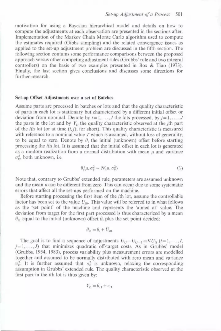
motivation for using a Bayesian hierarchical model and details on how tocompute the adjustments at each observation are presented in the sections after.Implementation of the Markov Chain Monte Carlo algorithm used to computethe estimates required (Gibbs sampling) and the related convergence issues asapplied to the set-up adjustment problem are discussed in the fifth section. Thefollowing section contains some performance comparisons between the proposedapproach versus other competing adjustment rules (Grubbs' rule and two integralcontrollers) on the basis of two examples presented in Box & Tiao (1973).Finally, the last section gives conclusions and discusses some directions forfurther research.

Set-up Offset Adjustments over a set of Batches

Assume parts are processed in batches or lots and that the quality characteristicof parts in each lot is stationary but characterized by a different initial offset ordeviation from nominal. Denote by /= 1 / the lots processed, by /= 1 Jthe parts in the lot and by K,; the quality characteristic observed at theyth partof the ith lot (or at time (ij), for short). This quality characteristic is measuredwith reference to a nominal value 7" which is assumed, without loss of generality,to be equal to zero. Denote by 0, the initial (unknown) offset before startingprocessing the /th lot. It is assumed that the initial offset in each lot is generatedas a random realization from a normal distribution with mean ^ and varianceo"e, both unknown, i.e.

0,\^.a'o^N(fUG'o) (1)

Note that, contrary to Grubbs" extended rule, parameters are assumed unknownand the mean /i can be different from zero. This can occur due to some systematicerrors that affect all the set-ups performed on the machine.

Before starting processing the first item of the /th lot. assume the controllablefactor has been set to the value f/ o- This value will be referred to in what followsas the 'set point' of the machine and represents the 'aimed at' value. Thedeviation from target for the first part processed is thus characterized by a meanOil equal to the initial (unknown) offset 0; plus the set point decided;

The goal is to find a sequence of adjustments Ujj— Ujj^ ^=VUij (/= 1, . . . , /,7 = 1 , . . . , / ) that minimizes quadratic off-target costs. As in Grubbs' model(Grubbs, 1954, 1983), process variability plus measurement errors are modelledtogether and assumed to be normally distributed with zero mean and varianceaf.. It is further assumed that (rf. is unknown, relaxing the correspondingassumption in Grubbs' extended rule. The quality characteristic observed at thefirst part in the ith lot is thus given by:


where y,, '-^N{Q.GI) represents random error. Once the quality characteristic hasbeen observed, the adjustment V(/,i = f n —^/o has to be determined andimplemented in order to 'cancel' the offset f?,i. i.e.

where Qn is an estimate of the offset of the current lot (lot /) after obtaining themeasurement for part 1. Due to this adjustment, the mean of the qualitycharacteristic for the next processed part changes to:

and the quality characteristic observed for the second part in the lot is given by:

Continuing in this way. the quality characteristic of the yth part processed in the(th lot is given by:

Yu-O.^ + û (2)

where:

fl,7 = ô--i+Vf/,,-_i (3)

and 0,0 = î- Hence, the next adjustment is selected as:

Therefore, adjustments Vt ,j can be determined by estimating the relevantunknown parameter; in this case, the mean of the quality characteristic in thecurrent lot, based on data available up to time (ij).

An important relationship in the problem of estimating the means in a one-wayrandom effects model can be seen after some manipulations in expressions (2)to (4). Solving recursively equation (3) and considering that Vt/jj= t/,-^—t/ij_i,the mean of the quality characteristic can be rewritten as:

O,.. = (j,. + f/,..,, (5)

Therefore, the quality characteristic of the /th part in the /th lot can berewritten as:

> . = 0. + f/,,_j + .,.. (6)

Considering that at the time Y^ is observed, f/jj-i is known, a new variable Xjjcan be defined as:

Merging the last expression with equation (1) permits us to derive an analogywith a one-way random effects model, i.e.,

(8)

Set-up Adjustment of a Process 503

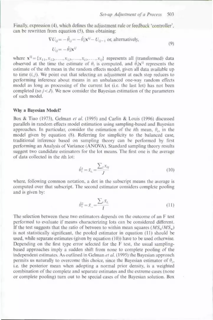
Finally, expression (4), which detines the adjustment rule or feedback 'controller',can be rewritten from equation (5), thus obtaining:

VUtj=~djj= -Oi\\'^- Uij^i or, alternatively,

/"/..= —f)-\\''

where x '^= {.YI[, .YI2. . . . , . V ] ; , . . . . .Y,I , . . .,-v,-j} represents all ( transformed) dataobserved at the time the estimate of 0, is cotnputed. and OJx'J represents theestimate of the /th mean in the random effects model, given ail data available upto time (/,/). We point out that selecting an adjustment at each step reduces toperforming inference about means in an unbalanced one-way random etfectsmodel as long as processing of the current lot (i.e. the last lot) has not beencompleted (so j<J). We now consider the Bayesian estimation of the parametersof such model.

a Bayesian Model?

Box & Tiao (1973). Gelman et al. (1995) and Carlin & Louis (1996) discussedparallels in random effects model estimation using sampling-based and Bayesianapproaches. In particular, consider the estimation of the /th mean, 0^, in themodel given by equation (8). Referring for simplicity to the balanced case,traditional inference based on sampling theory can be performed by firstperforming an Analysis of Variance (ANOVA). Standard sampling theory resultssuggest two candidate estimators for the lot means. The tirst one is the averageof data collected in the /th lot:

(10)

where, following common notation, a dot in the subscript means the average iscomputed over that subscript. The second estimator considers complete poolingand is given by:

< 5 ? = . v . . = ^ (U)

The selection between these two estimators depends on the outcome of an F testperformed to evaluate if means characterizing lots can be considered different.If the test suggests that the ratio of between to within mean squares (MSJMS^)is not statistically significant, the pooled estimator in equation (II) should beused, while separate estimates (given by equation (10)) have to be used otherwise.Depending on the first type error selected for the F test, the usual sampling-based approaches imply a sudden shift from none to complete pooling of theindependent estimates. As outlined in Gelman et al. (1995) the Bayesian approachpermits us naturally to overcome this choice, since the Bayesian estimator of ^,.i.e. the posterior mean when adopting a normal prior density, is a weightedcombination of the complete and separate estimates and the extreme cases (noneor complete pooling) turn out to be special cases of the Bayesian solution. Box


& Tiao (1973, p. 388) pointed out how this has a parallel with certain results insampling theory, specifically with the work of James and Stein.

The Bayesian approach has some additional advantages over the samplingapproach, related to the estimation of variance components, and to flexibility indepartures from assumptions. Variance components estimates can be useful inadjusting for initial offsets. After some lots have been processed, estimates ofbetween-lots and within-lot variances, i.e. af, and CT^. can be obtained andGrubbs" extended rule can be adopted thereafter. Considering the estimation ofthe variance components, traditional sampling theory suggests using:

(12)and

^ (13)

The first well-known problem concerns IT|, which turns out to be negative ifMSy,<MS^ Furthermore, the estimate aj given by equation (13) has a complexdistribution that induces problems in deriving a confidence interval for thisquantity. In contrast, the Bayesian approach permits us easily to tackle the lackof normality and/or independence and possible heterogeneity of variances (Box&Tiao, 1973).

Due to the considerations outlined above, a Bayesian approach has beenadopted for determining the adjustments for an on-line set-up adjustment in alot-by-Iot production process.

Bayesian Online Adjustment of Initial Offsets

From a Bayesian perspective, the one-way random eflects model is a special caseof a hierarchical model used in describing multiparameter problems in whichparameters are related based on some structure that depends on the specificproblem addressed.

The Bayesian model used for the set-up adjustment problem can be describedby considering the case when the^th part in the (th lot has been just processedand we have to decide the adjustment for the next part in lot /. In this case, thefirst stage of the hierarchy models the distribution of data conditionally onunknown parameters and is given by the first equation in (8). In this equation,the (transformed) data distribution is given conditionally on two unknownparameters: the current mean f?, and the variance within lots a^.. The secondstage in the hierarchy specifies the distribution of these unknown parameters.The within-lot variance (T , which represents process variability plus measurementerrors, does not depend on any other parameter. Therefore, the probabilisticspecification of this parameter at the second stage of the hierarchy models theprevious or subjective knowledge on it. i.e. its prior distribution. Adoptingconjugacy at each step of the hierarchical model (a common choice for therandom effects model, Gelfand et al.. 1990; Gelfand & Smith, 1990), the priordistribution for o^. is given by:


fo r (k lN1 : i }

Figure 1. Graphical representation of the three-stage model A/,, where T,, — I/IT," andr,j \loj are ihe precisions of the two normal distributions in the model

where IG represents an Inverse-Gamma distribution and Ui^bj are assumedknown and have been chosen both equal to 0.001 to model 'vague' priorinformation (Spiegelhalter et al., 1994).

The second unknown parameter, modelled at the second stage in the hierarchyis the initial offset fi,. given by equation (I). As it can be observed, its distributionis given conditionally on the other two parameters, {.i and af,. These arehyperparameters and are modelled at the third stage in the hierarchy, where theprior distributions on them is reported. Adopting once again conjugacy, priorson these hyperparameters are given by:

U li|^ (Ta-^Niltfi tin) (15)

o"o|<7i, /jj " IG(a^. /jj) (16)

where IG is the Inverse-Gamma distribution and ^i,,. rr5,;/,, ^ are assumedknown. In particular, they were selected according to values suggested in theliterature (Spiegelhalter et al., 1994) to model 'vague' prior distributions, i.e.((, = 0, r7^-1.0£+10. (/i=/j, = 0.001.

The random effects model, hereafter called model A/,, can be described bythree stages modeUing respectively data, parameters and hyperparameters. Usingthis approach, the model A/ can be graphically represented as in Figure 1 andis given by the following.

Three-stage Hierarchical Model M^

• First stage: data X^p {k=\,. ...i and p^\ J) with distribution given bythe first equation in (8).


• Second stage: parameters 0^ {k = \, /) and al with distributions givenrespectively by equations (1) and (14).

• Third stage: hyperparameters /( and (TI with distributions given respectively byequations (15) and (16).

We point out the similarity between the assumed model and a 'normal means'model (Gelfand el f//., 1990). Once data from all lots are available, the normalmeans model allows for ditferent lot sizes and ditferent within-lot variances,whereas we assume a constant lot size and the same within-lot variance distribu-tion for all lots. Extension to such case is straightforward but is not addressedin this paper.

As already mentioned, the adjustment VL'',j can be computed using equation(9) once the deviation from target Y;J has been measured, i.e. it is based onestimating the initial otfset 0;. Using the three-stage hierarchical model, theestimator of f, is given by the expected value of the posterior distribution andcan be computed if at least two parts from different lots have been alreadyprocessed (otherwise the variance between lots aj cannot be estimated). There-fore, adjustments Vf/,j for lots starting from the second lot are given by:

'J, M,) / = 2 , . . . , /and,/= 1,. . . , J (17)

where conditioning on M^ means the estimation is computed using the randomeffects model A/[.

Notice how, when selecting the adjustment for they+ I part in the /th lot. wehave unequal lot sizes since for all the lots already processed (A'= 1,. . . , /— 1) Jentries are available (in accordance to our constant lot size assumption) whilefor the current lot ik^i) justy^y data have already been collected. However,lot sizes can be treated as equal by considering future data (i.e. /? = /- |-1, . . . , /)of the current lot / as if they were missing data (Spiegelhalter et a!.. 1994).

One main advantage of applying Bayesian hierarchical modelling is thepossibility to select the initial set-point f/,+ i o that has to be set on the machinebefore processing the tirst part in the next lot (lot /+1). In contrast, Grubbs'harmonic rule requires us to collect at least one (uncontrolled) observation ineaeh lot in order to set the controllable variable starting with the second part ineach lot. Using the hierarchical model described, the predictive distribution forthe offset in the next lot can be derived using information collected in all theprevious lots. Therefore, we can set:

U^,,o^-E(()Ui\^'\M,) for i^X...J (18)

where ('; +Jx'-'. M, is the posterior predictive distribution (Gelman el a/., 1995)of a future offset given all the data collected from previously produced lots.Similarly, as before, prediction can start from the third lot since at least two lotshave to be processed to start estimating the variance between lots.

To start adjusting in the first lot, a reduced two-stage model A/, was used.When only one lot is being processed, the initial offset Oi can be considered notas a realization from a random variable but simply as an unknown parameter.Hence, the three-stage model A/j 'collapses' into a two-stage model, describingthe data distribution at the tirst stage, and priors on unknown parameters at the


Figure 2. Graphical representation of the two-stage model A/j where i,,= l/a, is the precisionof the normal distribution in the model

second one. Therefore, the first stage in model M2 is given by the first equationin (8), just as in model M,. The second stage reports priors on the two unknownparameters (?, and o",-. The prior on the last parameter is given again by equation(14), and the prior on Oi is given by:

e,\H-rT',^N(^i.G'o) (19)

where now // and a^ are supposed known and chosen to model vague priorinformation on 0^, i.e. /< = 0 and GQ — l.OE-f 10. Therefore, the model for selectingadjustments in the first lot is the following.

Two-stage Hierarchical Model Mj

• First stage: data Xip(p = \,... ,7) distribution given by the first equation in (8).• Second stage: parameters Oi and a^ with distributions given respectively by

equations (19) and (14).

For the second model, the adjustments Vt/iy are obtained by computing theexpected value of the posterior distribution of 0^, given data already observedand the model M2, i.e.

t/j .= -E(O,\x^\ A/2), y = 2, 3, . . .,y (20)

where j starts from 2 since at least two parts have to be processed to estimatethe within-lot variance af.. To start adjusting just after the first part in the firstlot is processed and measured, the trivial estimator:

f / u = - - v u (21)

can be used, which coincides with Grubbs' harmonic rule. In summary, theproposed adjustment procedure consists of computing the adjustments asreported in Table 1.

Batch

123 . . . I

lable 1.

U,o

00

equation

Bayesian

(18)

adjustment

equation

of initial ofTset over a set of lots

^'.

(21) for7=l and equation (20) for^^equation (9) for J= I , . . . ,7equation (9) for /= 1, f

2 J


Gibbs Sampling Implementation and Convergence Issues

Although Bayesian models permit us to overcome the difficulties implied bysampling theory and to derive easy extensions to more complex problems., it iswell-known that their main drawback is related to computational difficulties inthe calculation of marginal posterior densities required for Bayesian inference.Problems exist related to the exact computation of functions of the marginalposterior densities since they require solving complicated high-dimensionalintegrals. In the last two decades, these difficulties have been greatly reduced dueto the development of simulation-based approaches (Gelfand & Smith, 1990),which permit us to numerically compute marginal posteriors. In particular,Markov Chain Monte Carlo methods are widely spread and consist of performingMonte Carlo integration using Markov Chains. One of the better known MCMCalgorithms used to construct this chain is the Gibbs sampler. The basic ideas ofthe Gibbs sampler applied to the adjustment problem at hand are summarizedin Appendix Al.

A complete implementation of a Gibbs sampler requires dealing with conver-gence issues. In particular, it is necessary to specify the variables ! (truncationpoint) and m (stopping point) in equation (28) in Appendix Al. The first ofthese variables represents the number of iterations that are required to reach thesteady-state (i.e. the approximately true) distribution. The / variable constituteswhat is called the burn in period in which observations have to be discarded forcomputing moments of the posterior marginal densities. This represents thetransient period during which the Markov Chain has not reached stability andis thus highly influenced by starting points (initial values of the parameters thathave to be estimated).

The second variable, m, is the total number of iterations, and is required todetermine the additional number of samples m — t that have to be drawn afterconvergence has been reached in order to compute all relevant moments of theposterior distribution (equation (28)). This variable is critical due to the Markovnature of the algorithm. If convergence has been reached, all the samples areidentically distributed. However, since the samples are autocorrelated, the slowerthe simulation algorithm in moving within the sample space, the higher thenumber of samples required to obtain efficiently the required estimates. Althoughtypical choices in the literature (/ —1000 and m= 10000) have been shown to beappropriate for many applications, we use convergence diagnostic algorithmsproposed in the literature to evaluate whether these values are satisfactory forthe adjustment problem. These convergence diagnostic algorithms are brieflydescribed next. This is followed by a discussion of the software implementationof the proposed approach to the set-up adjustment problem.

Convergence Diagnostic Algorithms and their use in the Adjustment Problem

Although theoretical results, oriented to define ex ante the number of iterationst required to reach convergence, appear to be a promising solution to deal withconvergence issues in MCMC, the results obtained in this field are far frombeing actually applied due to their mathematical complexity and the excessive

Set-up Adjustment of a Proeess 509

calculation involved (Cowles & Carlin. 1995). Thus, most of the apphed workon MCMC focuses on using a set of diagnostic tools for assessing convergenceby analysing output produced by MCMC simulations. Numerous studies (e.g.Brooks & Roberts, 1998; Cowles & Carlin. 1995) have compared the convergencediagnostics proposed in the literature over a set of problems in order to rankthem. Since, at this time, no diagnostic algorithm seems globally superior to allothers, we follow the recommended approach of applying simultaneously morethan one diagnostic method to assess convergence of the lot mean estimatesneeded for adjustment at each point in time (/,/). In particular, we use two ofthe most popular methods adopted in the literature, proposed by Raftery &Lewis (1996) (RL) and Gelman & Rubin (1995) (GR).

The first algorithm (RL) is based on monitoring the autocorrelation withinone single chain. It requires as input the quantile q of the posterior distributionthat has to be estimated to within ± r with probability .v. Default values suggestedby Raftery & Lewis are £/ = 0.025, r = 20%; ^ = 0.005 and ^ = 0.95. Since theadjustment selection requires computing the posterior mean, the 0.5 quantile(median) has been selected as reference. Accuracy has been defined accordinglyas 10% of the desired quantiie, thus obtaining r= 10%, (7 = 0.05. Concerning s,the value 5 = 0.95, suggested by Raftery & Lewis, has been utilized.

The RL algorithm has the main drawback of masking excessive slow conver-gence of Markov Chain simulation, a problem common to other methods basedon a single simulated chain. It could happen that, looking at one single chain,convergence seems achieved although the chain is stuck in one place of the targetdistribution. In order to overcome this problem, Gelman & Rubin (1992, seealso Gelman, 1995) suggest performing multiple simulations, starting fromdifferent initial values for parameters that have to be estimated. These valueshave to be chosen to be 'overdispersed' with reference to the target density. Sincethe target density is not known in advance, sometimes this technique has beencriticized for the lack of guidelines about selecting the starting points. In ourprocess adjustment application, however, this choice can be easily performed,considering a basic knowledge of the process producing the quality characteristic.For example, a rough idea of the process capability can give information on therange of variation (at least its magnitude) of the quality characteristic and thisinformation can easily be used in determining overdispersed initial values forparameters derived through MCMC.

Once starting values are selected, the GR algorithm is based on mixingsimulated chains and comparing the variance within each chain to the totalvariance of the mixture of chains. These (estimated) variances permit us to derivethe 'estimated potential scale reduction' factor R. As simulations converge, Rdeclines to 1, thus assessing that parallel chains are essentially overlapping. Therule of thumb suggested when performing the GR diagnostic is to continuesimulation until R is close to one; for example, lower than 1.2. In the set-upadjustment application, diagnostics are run on the simulated lot mean ( ,)corresponding to the current lot (/).

Using both diagnostic algorithms briefly described, the proposed set-up adjust-ment approach can be summarized as follows. After the first part is processed inthe first lot and the first trivial-value b\] = — .Y, , is set on the machine, the second

510 B. M. Colosimo Qi al.

part in the first lot is processed and A-, is observed. Therefore, adjustment t/,2has to be selected according to equation (20). The expected value required isthus computed through MCMC. Starting from the trial values suggested in theliterature (r=1000 and m = 10000) two MCMC chains are simulated, each onestarting from different initial values, as previously mentioned. Then, the RL diag-nostic check is performed on each chain for 6^, the parameter of interest. If theRL algorithm suggests for one of the chains, higher / or tn values (i.e. convergencediagnostic has failed thus far), MCMC is rerun for both chains using the new r, mparameters suggested by RL. To avoid an excessive number of reiterations, thesevalues are rounded to the upper multiple of 500 for t and the upper multiple of5000 for m (thus increasing / and m in steps of 500 and 5000, respectively). Hence,MCMC simulations and RL convergence checks are performed again until thediagnostic check is satisfied. Starting with the values eventually assessed for t andm. the GR diagnostic is then performed on both chains (for ('i).

Similarly as for the RL algorithm, if the GR method concludes that conver-gence has been reached, i.e. the estimated potential scale reduction factor^^1 .2 , an adjustment is computed by calculating the expected value of theposterior distribution of Q^ obtained from the two final MCMC chains. Other-wise, t and m are increased. Contrary to the RL diagnostic, the GR algorithmdoes not suggest new values for these parameters, so both are increased (in stepsof 500 for r and 5000 for /»). Both chains are thus simulated again and the GRcheck performed until the algorithm permits us to conclude that convergencehas been reached and to set (7,2 is possible. We then proceed to compute t/,3and so on until we process all parts in all lots.

Computer Implementation of the Proposed Approach

All the steps in the previous section are performed for each adjustment, andcomputed following Table 1. A Visual Basic (VB) code has been written tosimulate the determination of the adjustments over a set of lots. Each time anadjustment has to be computed at time (/,/), the code launches the execution ofboth the MCMC simulations and the convergence checks. The MCMC simula-tion is coded in the Buys {Bayesian inference Using Gihbs Sampling, Spiegelhalteret al., 1994) language, while the RL and GR convergence diagnostic algorithmsin the CODA Hbrary (Best et al., 1995) are used running under R, the freelyavailable version of S-plus. After MCMC convergence is assessed, the adjustmentis computed and all input files required to rerun MCMC simulation for the nextadjustment are automatically generated by the VB program.

With respect to computational time, the software requires a few seconds toperform each MCMC simulation and around half a minute to perform eachconvergence check, on a Pentium II 333 MHz. However, due to the use ofditferent available software packages, most of the computational time is due towriting and reading MCMC output, considering that each chain is constitutedby thousands of values. Therefore, a specific code written to perform MCMCand convergence checks, maintaining in memory all these values of the chains,should significantly improve computational times. For most high value-addeddiscrete part manufacturing processes, we envisage the MCMC adjustment


approach being applied, and the aforementioned computing times should beadequate, that is, well below the time between consecutive parts as they areproduced in a manufacturing process. The present version of the softwareperforms the different MCMC simulation chains and the convergence checkssequentially, so computational times could be reduced by simulating differentchains on parallel processors.

Two Examples of Sequential Bayesian Set-up Offset Adjustment over a Set ofLots

Bayesian adjustment of an initial or set-up offset is useful when several lots haveto be processed but no information is available on parameters characterizingoffset and process distributions. Alternative feedback methods that can be usedin this case are the harmonic rule due to Grubbs (1983):

, -j}^, (22)

(with Uio = O) and the integral controller (Box & Luceno, 1997J:

S/U^i^-?.Y;j (23)

(with U,o = 0) since both these rules do not require any information on offset orerror distributions (Del Castillo et al., 2002b). The performance obtained withthe MCMC-based adjustment method has been compared with the performanceof these competitor rules considering two examples. Both examples were pre-sented by Box & Tiao (1973) in the framework of Bayesian estimation in a one-way random effects model and are reproduced in Table 2. The first examplerefers to the yield of dyestuff measured from five samples taken from six batchesof raw material, while the second one relates to randomly generated data with// —4, rT,) = 2 and rr,, — 4. This was used by the authors to study the Bayesianestimation of variance components in a case where sample-based theory deter-mines a negative estimate ol' df, obtained with equation (13) where MSi,<MS^For illustration purposes of the online MCMC adjustment approach, we pretend

Table 2. First example: dyestutT data F , for /= 1,..., 6 and 7= 1,..., 5 (yield of dyestulT ingrams of standard colour computed with respect lo larget value of 1400 g). Second example:

data with fi=4, a,, = 2 and fT,=4 (Box & Tiao. 1973)

Batch

123456

154515401595144515951520

First

144015551550144016301455

example

144014901605159515151450

152015601510146516351480

158014951560154516251445

Batch

123456

7.2985.220.112.2120.2821.722

Second

3.8466.55610.3864.8529.0144.782

example

2.4340.60813.4347.0924.4588.106

9.11.5.9.9.0,

56678851288446758

7.99-0.8928.1664.987.1983.758

512 B. M. Colosimo Qt a\.

Table 3. Initial values and seeds for the random generation adopted in the two MCMC chainssimulated at each step of the adjustment procedure for both the examples

Chain

FirstSecond

2000-2000

0.0011000

0.0011000

Seed

105612656111235

the data become available sequentially in time and apply the MCMC adjustmentprocedure at each time instant.

Two MCMC chains were simulated at each step of the adjustment procedureand different initial values of the parameters that have to be estimated(/i, (TJ, af. and Oj, where / = 1. . . . , 6 for the model M^; cf. and ('i for the modelM2) were specified for each chain. Among these parameters, the Ofi in modelA/i and (9, in model Mj can be randomly generated by the software, usingequations (1) and (19). respectively. To make this random generation differentfor the two chains, a different seed must be specified for each chain. Initial valuesand seeds used for both examples are reported in Table 3. To see how the effectof these starting values disappear as the MCMC simulation proceeds, considerthe plot shown in Figure 3. It represents the first 600 iterations of the twoMCMC chains estimating (J, in adjusting the second part of the third lot for thefirst example. As can be observed, the two chains start respectively around 2000and —2000 (their mean values) and have almost 'forgotten' these starting pointsafter 100 iterations. The trial value adopted, i.e. /=1000, was observed to beadequate for all the simulations performed with the first data set while anincrease to only t= 1500 was required for the second case studied. With respectto the total number of runs m, it was started from the trial value of 10,000.Owing to high autocorrelation of the chains, it was increased as suggested byconvergence algorithms to the final values of 45,000 and 20.000 for the first andthe second examples, respectively.

-3000

First chain

Second chain Iteration

100 200 300 400 500 600

Figure 3. First 600 iterations of the two MCMC chains simulating (1^ in adjusting the secondpart in the third lot for the first example


Adjustments were computed with the proposed procedure for all the lotsprocessed in the two examples. After the 30 adjustments were computed, aquadratic symmetric loss function, given by:

ft 5

c=y y Yfj (24)

was used to compare the performance obtained with this approach versusGrubbs' harmonic rule and two discrete integral controllers (or EWMA control-lers) with different weights A = 0.1 and A = 0.4. These weights were chosen as theycover the range of EWMA weights recommended in the process adjustmentliterature (Box & Luceno, 1997). Large values of A (i.e. closer to 1) will bringthe process back to target faster on average, but will increase the variance of thecontrolled process (Del Castillo, 2001), also increasing the cost function (24).

Figure 4 reports the pattern of deviations from target Y^ for the dyestuff data(first example) observed in each lot using Grubbs' harmonic rule, the MCMC-based adjustment method, and the two EWMA controllers (with A = 0.1 and 0.4.respectively). As can be observed, the deviations from the target induced by theMCMC approach are smaller than the ones due to the other rules, especiallyafter the first two lots have been machined, i.e. after information on the variancebetween lots becomes available.

The deviations from target K,j observed for the second example in each lotusing the four competing rules are reported in Figure 5, which, as before, testifiesto the better performance of the MCMC approach compared with the otheradjustment rules, especially after the first two lots have been processed.

Global savings in costs attained in each lot using the MCMC-based approachversus Grubbs' rule and the two EWMA controllers are reported in Figure 6 forboth the examples studied. As can be observed, savings in costs are almostalways positive, showing that the MCMC approach outperforms the competitoradjustment rules considered. Furthermore, the three alternative methods can beranked, noting that savings induced by the MCMC approach decrease goingfrom the FWMA controller (;. = 0.1) to the other EWMA controller (;. = 0.4)and eventually to Grubbs' adjustment rule. This ranking is even more clearconsidering the total costs C obtained by applying the different adjustment rulesto the two examples considered (Table 4). As can be observed, percentageadvantages determined by the MCMC Bayesian procedure vary from 27% to63'M) for the first example and from 18' !) to 50% for the second one. The savingsare mainly due to the ability to predict the initial offset before starting a new lot.

Discussion and Further Research

This article presented a procedure to adjust the set-up errors of a productionprocess over a set of lots assuming a one-way random effects model (withunknown parameters) for the initial offset in each lot. The approach presentedis based on repeatedly estimating the initial offset in each lot through MarkovChain Monte Carlo simulation of a Bayesian hierarchical random effects model.Assuming a quadratic off-target cost model, the approach presented was com-


200150100

50

0

-50-100-150

250200150100500

-50-100

First Lot Second Lot

" ' • \

Third Lot

- - ^ ^s A \o--" ..a\

. • - ' ' • • \

' ^ ^ 3 s

\ ^

V4 . - ^-^

Fourth Lot

2OO1

150

100-50-0

- 5 0 -

-100-

-150-

Fifth Lot150'

100-

50-

0

- 5 0

-lOO-"

Sixth Lot

\ 2\

4..-D-.

• " • n

- Grubbs • MCMC EWMA(O.I) --<?— EWMA(0.4)

Figure 4. Deviations Irom tyrget K,,- obtained using Grubbs' harmonic rule, the MCMCapproach and the iwo EWMA controllers (with /^O. l and 0.4} to adjust an initial offset for

the dyestuff data {Table 2)

pared with adjustment rules that can be applied when parameters of theinitial offset distribution are unknown, i.e. Grubbs' rule (based on stochasticapproximation) and discrete integral controllers (or EWMA controllers). Theprocedure was illustrated with application to two examples presented in theliterature (Box & Tiao. 1973) where the advantages attained with the approachpresented here vary from 18'Mi to 27'Mi and from 29'Vij to 37% when consideringGrubbs" rule and the best EWMA controller utilized (A = 0.4). respectively. Theproposed approach for set-up adjustment can be applied to high value added,short-run manufacturing processes, where the computational expense and relativecomplexity of the proposed adjustment rule, compared with the simplicity of thealternative rules studied, can be justified.

Recent work by Box & Luceiio (2002) considers a problem similar to themachine set-up problem discussed herein, but with some important differences.

86420

-2-4-6

First Lot

i>-^~;r:S


Second Lot

14121086420

- 2- 4- 6

1086420

-2-4-6

Third Lot

Fifth Lot

10-,8-6-4-20

-2--4--6-

Fourth Lot

— Grubbs •a M C M C EWMA(O.I) - - O — EWMA(0.4)

Figure 5. Deviations from target F,j ohtiiined using Grubbs" harmonic rule, the MCMCapproach and the two EWMA controllers (with A = 0.1 and 0.4) to adjust an initial offset for

the second example {Table 2)

In Box & Luceno's problem, the set-up error is assumed to be caused byvariability in the different feedstock material used in each batch. These authorsthen show how the feedstock material can be measured and these data used in afeedforward adjustment scheme to anticipate changes that occur between lots,and in this way complement the feedback action of an integral controller. Theyalso consider a non-stationary disturbance (IMA(1,1)) to model within lotvariability, and consider adjustment costs. Interestingly, the MCMC-basedadjustment strategy achieves the benefits of feedforward control, i.e. anticipationof the set-up error and the possibility to adjust for the first part in each lot, onceenough batches have been processed to allow for reliable parameter estimates.Although the set-up adjustment problem focuses on high-value discrete-partmanufacturing processes, where the dominant cost is the off-target cost andwhich do not follow non-stationary processes if uncontrolled, it would be worthexploring MCMC-based methods applied to Box & Lucefio's "feedstock change'problem. This would be of particular use in continuous manufacturing processes


AC:

120000n

100000-

80000-

60000-

40 0001

20000-

0-

-20000-

y

o""1

First example A

A/\ \/ \ / \

2 3 4 5 6 i

200 n

150

100-

50-

Second example

0-

-50-1

— • - - Grubbs

2

—A>—

3

- EWMA(O.I)

•-

4 5 6 i

— 0 — EWMA(0.4)

Figure 6. Savings in costs per each lot AC, = Cf"""''"'" rui._ ^ MCMC obtained with the MCMCapproach versus allernalive rules, i.e. Grubbs' harmonic rule and two EWMA controllers—

with /.-O.I and 0.4

Table 4. Costs C (equation (24)) related to the different adjustment rules and percentagesavings AC'/o induced by the MCMC-based approach over the other rules for the two examples

Adjustment rule Costs C AC'A,

First example

Second example

MCMCGRUBBS

EWMA(/-0.4)EWMA(/-O.I)

MCMCGRUBBS

EWMA(A=0.4)

EWMAU-Ol)

160982.39221316.15254072.75437815.98

533.27649.27745.95

1072.52

27%37%63%

18%29%50'^

where both process and disturbance dynamics frequently occur, and when theprocess parameters are not necessarily known.

The preliminary performance results of the previous section indicate that initialdirection for further research should be to extend the numerical comparisons inorder better to understand the effect of different factors (such as the lot size, the


number of lots, the parameters characterizing the initial offset distribution) onthe advantages obtained with the Bayesian approach. As previously mentioned,a further direction concerns the situation where the number of (small) lotsprocessed is relevant. In this case, it is possible to estimate the unknownparameters through MCMC and plug in these estimates in a simpler adjustmentrule that assumes known parameters, e.g. in Grubbs' extended rule. The perfor-mance of such a simpler rule remains a matter of study.

Taking advantage of the flexibility of hierarchical models, a further directionof research could be related to different extensions of the presented approachto model situations that can arise in short-run manufacturing. As examples,measurement errors or tool wear can be easily included in the study, adding astage in the hierarchy and relaxing the assumption of i.i.d. random errors,respectively.

Acknowledgements

This research was partially funded by NSF grant DM I 0200056.

References

Best, N. G.. Cowles. M. K. & Vines. S. K. 0995) CODA Manual Version O.JO (Cambridge: MRCBiostalislics Unit).

Box. G. E. P. & Luceno. A. (1997) Statistical Control bv Monitoring and Feedback Adjustment {New York:Wiley).

Box, G. E. P. & Luceno, A. (2002) Feedforward as a supplement to feedback adjustment in allowing forfeedstock changes, Journal of Applml Statistics, 29(8), pp. 1241-1254.

Box, G. E. P & Tiao, G. D. (1973) Bayesian inference in Statistical Analysis (New York: Wiley).Brooks, S. P. & Roberts, G, O. (1998) Assessing convergence of Markov Chain Monte Carlo algorithms.

Statistics and Computing. 8, pp. 319-335,Carliii. B. P. & Louis. T. A. (1996) Bayes and Empirical Bayes Methods for Data Analysis (London:

Chapman & Hall).Cowles. M. K. & Carlin. B. P (1995) Markov Chain Monte Carlo convergence diagnostics: a comparative

review. Journal of the American Statistical Association. 91. pp. 883-904.Del Castillo, E. (2001) Some properties of EWMA feedback quality adjustment schemes for drifting

processes, Journal of Quality Technology. 33(2). pp. 153-166.Del Castillo, E.. Pan. R. & Colosimo, B. M. (2003a) An unifying view of some process adjustment

methods, Journal of Quality Technology, 35(3). pp. 286-293.Del Castillo, E,. Pan, R. & Colosimo. B. M. (2003b) Small sample comparison of some process adjustment

methods. Communications in Statistics. Simulation mtt Computation. 32(3). pp. 923-942.Gelfand, A. E. & Smith, A. F. M. (1990) Sampling-based approaches to ealculating marginal densities.

Journal of the American Statistical Association. 85(410). pp. 398^09.Gelfand, A. E., Hills, S. E.. Raeine-Poon. A. & Smith. A. F. M. (1990) Illtistration of Bayesian inference

in normal data models using Gibbs sampling. Journal of the American Statistical Association 85(412).pp. 972-985.

Gelman. A. (1996) Inference and monitoring convergence, in: W. R. Gilks, S. Richardson & D. J.

Spiegelhalter (Eds) Markov Chain Monte Carlo in Practice, pp. 131-140 (London: Chapman & Hall).Gelman, A. & Rubin. D. (1992) Inference from iterative simulation using multiple sequences. Statistical

Science. 7, pp. 457 511,Gelman, A.. Carlin, J. B.. Stern, H. S. & Rubin, D- B. (1995) Bayesian Data Analysis {London: Chapman

& Hall).


Gilks. W R., Richardson. S- & Spiegelhalter, D. J. (Eds) (1996) Markov Chain Monte Curio in Praciice(London: Chapman & Hall).

Grubbs, R E, (1954, 1983) An optimum procedure for setting machines or adjusting processes, IndustrialQuality Control. July, reprinted in Journal of Qtuility Technology. 1983, I5|4), pp. 186 189.

Ral'tery, A. E. & Lewis, S. M. (1996) Implementing MCMC, in: W. R. Gllks, S. Richardson and D. J.Spiegelhalter (Eds) Markoi Chain Monte Carlo in Practice, pp. 115-130 (London: Chapman & Hall).

Spiegelhalter. D. J., Thomas, A., Best, N. G. & Gilks, W. R. (1994) BUGS: Bayesian inference Using GihhsSampling, version 0.50 (Cambridge: Medical Research Council Biostatistics Unit).

Sullo, P, & Vandeven, M. (1999) Optimal adjustment strategies for a process with run-to-run variationand 0-1 quality loss, HE Transactions. 31, pp. 1135-1145.

Trietsch, D. (1998) The harmonic rule for process setup adjustment with quadratic loss. Journal of QualityTechnology. 30(1), 75-84.

Appendix Al: Gibbs Sampling in the One-way Random Effects Model

To estimate all the unknown parameters and hyperparameters in the randomeffects model, the Bayesian approach requires us to assume a set of priordistributions. A common choice for the random effects model (Gelfand el al.,1990; Gelfand & Smith, 1990) is adopting conjugacy at each step of thehierarchical model, thus assuming:

(25)

where /^o, CQ, « I , ^ J . Ui, 3 are assumed known. In particular, a,. A, (and/or Ui,hj) can be assumed equal to 0 to model the usual improper prior for aj [al) anda vague prior for jx can be assumed by setting al sufficiently great, e.g. CTQ^ lO'' .

If all the observations from all lots X" = (A-,J. / = 1 . . . . , / ;y= 1 J) have beencollected, inference on the unknown parameters can be performed as follows.Due to conjugacy adopted at each step, all the full conditional posteriors can bederived as follows (Gelfand et al.. 1990):

(26)


^ = 2 ; y x'- = {v

1 is a / x 1 column vector of Is and I is the / x / identity matrix. Althoughsimilar to the random effects model, the process adjustment problem focuses onthe lot means f?, as the parameters of interest, rather than on the variancecomponents. The conditional posteriors can be all expressed in closed form asin equation (26). but the computation of the marginal posteriors requires solvingcomplex high-dimensional integrals.

Introducing a more general notation, assume that the hierarchical modelrequires the estimation of K parameters W = {IVi, IV2,..., Wf^), which aremodelled as random variables in the Bayesian framework. In the random effectsmodel. K=f-\-?>, i.e. the / components of 9. fu Cr and (rf,. Due to conjugacy(although this is not a required hypothesis for the computational approachdescribed) all the full conditional posteriors

can be assumed known. To estimate each parameter W^, the marginal posterior/7(vij,x'O has to be computed.

Markov Chain Monte Carlo methods can be used to estimate these posteriormarginals. In particular, one of the most powerful MCMC methods is the GihhsSampler, which has the relevant advantage of being almost independent of thenumber of parameters and stages in a hierarchical model. Consider the generalproblem of estimating K parameters W= li^i. W,,..., Wf^ and assume that thefull conditional distributions /?(vi |n-, ^), k^\ ,K, are all given. Given anarbitrary set of starting values (Wf\ Wf^ W^K^), the first iteration in Gibbssampling is performed as follows:

Draw

Draw

Draw W^^^ -pin-^l ^?\..., ^^K- 1)

thus obtaining, as a result, a set of points (W\^\ HV* W *) that representthe starting values for the next step. Iterating the process in this case also, theconvergence is proved. Indeed, denoting with / the generic iteration of thealgorithm, it can be shown that:

(^r,,^i^„...,w^^)^/-(HVH^,...,vv^) (27)

Assume convergence has been reached after t steps, m — ( further samples can be


drawn and the marginal posterior density for each variable W^ can then becomputed as:

1 "'Pi^k)- , Z p,{W,\W,= Wf,k^r) (28)

which can be viewed as a 'Rao-Blackwellized' density estimator (Gelfand et ciL,1990).

A Sequential Markov Chain Monte Carlo Approach to Set-up Adjustment of a Process over a Set of Lots

Documents

Transcript of A Sequential Markov Chain Monte Carlo Approach to Set-up Adjustment of a Process over a Set of Lots