1 Open set, closed set, bounded sets, internal points ...
152
1 Open set, closed set, bounded sets, internal points, accumulation points, isolated points, boundary points and exterior points. 1 1 Open set, closed set, bounded sets, internal points, accumulation points, isolated points, boundary points and exterior points. Definition 1. Consider the set of real numbers R and let E ⊂ R be a subset of R. The following definitions are standard: ● A neighborhood of radius ε ∈ R, > 0, of a point x 0 of R is the set defined by: N ε (p)=(x 0 - ε, x 0 + ε) . A right-neighborhood of radius ε ∈ R, > 0, of a point x 0 of R is the set defined by: N ε (p) + =(x 0 ,x 0 + ε) . A left-neighborhood of radius ε ∈ R, > 0, of a point x 0 of R is the set defined by: N ε (p) - =(x 0 - ε, x 0 ) . ● A point p ∈ R is a limit point (also said accumulation point) of E if every neighborhood of p contains a point q ≠ p such that q ∈ E. In formula (p accumulation point of E ⊆ R) ⇔ (∀ε > 0 ⇒(N ε (p) E){p} ≠ ) The set made by all the accumulation point of E is called the derivative set and it is indicated with E ′ . ● If p ∈ E and p is not a limit point of E then p is called an isolated point of E. ● E is closed if every limit point of E is a point of E. For example the set E =(0, 1)⊂ R is not closed because the points 0 and 1 are limit points of E but they are not in E. Nevertheless the set E =[0, 1]⊂ R is colsed. ● A point p of E is an interior point of E if there is a neighborhood N ε (p) of p such that N ⊂ E. In formula (p interior point of E ⊆ R) ⇔ (∃ε > 0 ∶ N ε (p)⊂ E) ● E is open if every point of E is an interior point of E. For example the set E =(0, 1)⊂ R is open.
-
Upload
khangminh22 -
Category
Documents
-
view
1 -
download
0
Transcript of 1 Open set, closed set, bounded sets, internal points ...

1 Open set, closed set, bounded sets, internal points, accumulation points, isolated points, boundary points and exterior points. 1
1 Open set, closed set, bounded sets, internal points, accumulation points, isolated
points, boundary points and exterior points.
Definition 1. Consider the set of real numbers R and let E ⊂ R be a subset of R. The following
definitions are standard:
● A neighborhood of radius ε ∈ R, ε > 0, of a point x0 of R is the set defined by:
Nε (p) = (x0 − ε, x0 + ε) .
A right-neighborhood of radius ε ∈ R, ε > 0, of a point x0 of R is the set defined by:
Nε (p)+ = (x0, x0 + ε) .
A left-neighborhood of radius ε ∈ R, ε > 0, of a point x0 of R is the set defined by:
Nε (p)− = (x0 − ε, x0) .
● A point p ∈ R is a limit point (also said accumulation point) of E if every neighborhood
of p contains a point q ≠ p such that q ∈ E.
In formula
(p accumulation point of E ⊆ R)⇔ (∀ε > 0⇒ (Nε (p)⋂E) ∖ {p} ≠ ∅)
The set made by all the accumulation point of E is called the derivative set and it is indicated
with E′.
● If p ∈ E and p is not a limit point of E then p is called an isolated point of E.
● E is closed if every limit point of E is a point of E. For example the set E = (0,1) ⊂ R is not
closed because the points 0 and 1 are limit points of E but they are not in E. Nevertheless
the set E = [0,1] ⊂ R is colsed.
● A point p of E is an interior point of E if there is a neighborhood Nε (p) of p such that
N ⊂ E.
In formula
(p interior point of E ⊆ R)⇔ (∃ε > 0 ∶ Nε (p) ⊂ E)
● E is open if every point of E is an interior point of E. For example the set E = (0,1) ⊂ R is
open.

1 Open set, closed set, bounded sets, internal points, accumulation points, isolated points, boundary points and exterior points. 2
● E is bounded if there is a real number M and a point q ∈ R such that ∣p − q∣ < M for all
p ∈ E.
● A point p is a boundary point for E if every neighborhood of p contains at least one point
of E and at least one point in Ec.
The set made by all the boundary points of a set E is indicated with BE and it is called the
border of E. For example
B (0,1) = B [0,1] = B(0,1] = B[0,1) = {0,1} .
● A point p ∈ R is called an exterior point of E if
∃ε > 0 ∶ Nε (p) ⊂ Ec.
Recall that Ec is defined as the complement set Ec = R ∖E = x ∈ R∣x /i nE.
● The closure of E is defined as the set
sE = E⋃E′
that is the union of E with the set of all its limit points.
Remark. Trivially the closure of a set is always a closed set since it contains all its limit points by
definition.
Example. Consider the set E = (0,1). It is clear that
● E is open.
● The accumulations points are all the points of [0,1]
● All x ∈ (0,1) are interior points.
● All x ∉ [0,1] are exterior points, i.e all x such that x < 0 or x > 1.
● The numbers 0 and 1 are the boundary points.
● The set E has no isolated points.
Theorem 1.1. If S1, ..., Sn are open subsets of R then
n
⋂i=1
Si
is open.

1 Open set, closed set, bounded sets, internal points, accumulation points, isolated points, boundary points and exterior points. 3
Let I ⊆ N be an arbitrary set of indexes. Let Si be open for all i ∈ I. Then
⋃i∈I
Si
is open.
Proof.
1) Let x ∈ ⋂ni∈I Si, hence x ∈ Si for all i = 1, ..., n. Therefore given the openness of all Si, for all
i = 1, ..., n, there exists ρi > 0 such that Nρi (x) ⊂ Si. Consider ρ = mini ρi, hence for all i we have
Nρ (x) ⊆ Nρi (x) ⊂ Si hence Nρ (x) ⊂ ⋂ni=1 Si.
2) Let x ∈ ⋃i∈I Si. Therefore there exists i∗ ∈ I such that x ∈ Si∗ . Since Si∗ is open there exists a ρi∗
such that Nρi∗ ⊂ Si∗ ⊆ ⋃ni∈I Si.
Consider the sequence of open sets Sn = (1 − 1n ,1 +
1n) ⊂ R. Hence
S1 = (0,2) ⊃ S2 = (1
2,3
2) ⊃ S3 = (2
3,4
3) ⊃ ⋯
Now note that
● ⋂∞n=1 Sn = {1} is not open (in particular, since the set of limit points of {1} is empty, then {1}contains all its limit point so it is closed).
● ⋃∞n=1 Sn = (0,2) is open.
It is immediate to se that E is closed if and only if Ec = R/E is open. Hence
Theorem 1.2. If S1, ..., Sn are closed subsets of R then
n
⋃i=1
Si
is closed.
Let I ⊆ N be an arbitrary set of indexes. Let Si be closed for all i ∈ I. Then
⋂i∈I
Si
is closed.

2 Maximum, minimum, supremum and infimum of a subset of R 4
Proof. It follows from the fact that if S is closed then Sc is open and
(⋃i
Si)c
=⋂i
Sci .
Consider the sequence of closed sets Sn = [ 1n ,1 −
1n] ⊂ R. Now note that
● ⋃∞n=3 Sn = (0,1) is not closed (in particular, is open).
● ⋂∞n=3 Sn = [13 ,
23] is closed.
2 Maximum, minimum, supremum and infimum of a subset of R
In what follows, as before, we indicate with E a generic subset of R.
Definition 2. We say that M ∈ E is a maximum for E if
∀x ∈ E ⇒ x ≤M,
similarly we say that m ∈ E is a minimum for E if
∀x ∈ E ⇒m ≤ x,
Warning: it is not absolutely guaranteed that a set E has a minimum and a maximum! This is
mainly due to the fact that, in the definition of maximum and minimum, we require that both of
them belong to E. As an example consider E = (0,1). It is clear that ∀x ∈ (0,1) we have x > 0
and x < 1. Nevertheless 0 is not a minimum (neither 1 is a maximum) since it does not belong to
(0,1). In fact the open set (0,1) does not have neither a minimum nor a maximum. This is quite
easy to see: let x ∈ R, if x ≤ 0 or x ≥ 1, then x cannot be a minimum nor a maximum since x ∉ (0,1).On the contrary if x ∈ (0,1) then x is an interior point and so we can find elements of (0,1) that
are both below and above x, so x is neither a minimum nor a maximum.
Example. Consider the case
E = { 1
n∣ n ∈ N, n > 0} = {1,
1
2,1
3,1
4,1
5,⋯}
Note that 1 ∈ E and 1n ≤ 1 for all n ∈ N, so M = 1. Does the set E have a minimum point? The
answer is trivially no. Suppose that we have found a minimum point, and let 1n⋆ be such point.
Trivially1
n⋆ + 1< 1
n⋆,

2 Maximum, minimum, supremum and infimum of a subset of R 5
but 1n⋆+1 ∈ E so 1
n⋆ is not a minimum point.
Example. Consider
E = { 1
n∣ n ∈ N, n > 0} = {1,
1
2,1
3,1
4,1
5,⋯}
then ∄ the minimum of E, nevertheless
E′ = E⋃{0} = {0,1,1
2,1
3,1
4,1
5,⋯}
is such that 0 is the minimum point of E′. Similarly
F = {− 1
n∣ n ∈ N, n > 0} = {−1,−1
2,−1
3,−1
4,−1
5,⋯}
Then ∄ the maximum of F , nevertheless
F ′ = F⋃{0} = {0,−1,−1
2,−1
3,−1
4,−1
5,⋯}
is such that 0 is the maximum point of F ′.
Theorem 2.1. Maximum and minimum are unique (when they exist) Let E ⊂ R be a subset
of R. The maximum of E, provided that it exists, is unique. The same holds for the minimum.
Proof. Let M be a maximum of E. Suppose that M ′ is another maximum. Since M is a maximum
and since M ′ ∈ E then it must be M ′ ≤M . Nevertheless since, by hypothesis, also M ′ is a maximum
and since, by the definition of maximum, M ∈ E then it must be M ≤M ′. The only way in which
M ′ ≤M and M ≤M ′ are possible is M =M ′.
A more general definition is given introducing the concept of upper and lower bounds.
Definition 3. Let E ⊂ R. A number M ∈ R is called an upper bound for E if
∀x ∈ E ⇒ x ≤M.
Similarly, a m ∈ R is lower bound for E if
∀x ∈ E ⇒m ≤ x.
Note that, since the set R is provided with the “special” numbers ±∞ a lower and an upper bound
for any set always exist. In particular if E is bounded (see definition before) then both the upper
and the lower bound are ≠∞.
Example. Let E = (0,1). Then
● Any x ∈ R with x ≥ 1 is an upper bound.

2 Maximum, minimum, supremum and infimum of a subset of R 6
● Any x ∈ R with x ≤ 0 is a lower bound.
Example. Let E = (0,∞). Then
● Only +∞ is an upper bound.
● Any x ∈ R with x ≤ 0 is a lower bound.
Definition 4. Let E ⊂ R. Consider these two subsets
UE = {x ∈ R∣x is an upper bound for E} ,
LE = {x ∈ R∣x is a lower bound for E} . (2.1)
The minimum of UE (which always exists) is called supremum of E and it is indicated with supE.
The maximum of LE (which always exists) is called infimum of E and it is indicated with inf E.
Remark. Note that, differently from maximum and minimum, the supremum and the infimum
always exist, they could be however +∞ or −∞.
Remark. Note that, if E has a maximum element M then supE = M . Similarly, if E has a
minimum element m then inf E =m.
Example. Let E = (0,1). We already know that E has neither a minimum nor a maximum element.
However since
U(0,1) = {x ∈ R ∣ x ≥ 1}
then sup (0,1) = 1 and since
L(0,1) = {x ∈ R ∣ x ≤ 0}
then inf (0,1) = 0.
Remark. Thanks to Theorem 2.1 supremum and infimum of a set are unique.
Example. Consider the set
E = { 1
n∣ n ∈ N, n > 0} = {1,
1
2,1
3,1
4,1
5,⋯}
then
UE = {u ∈ R ∣ u ≥ 1} , LE = {` ∈ R ∣ ` ≤ 0}

2 Maximum, minimum, supremum and infimum of a subset of R 7
and so, although E has no minimum element, we have
inf (E) = max (LE) = 0,
while, straightforwardly, the maximum element and the supremum coincide
sup (E) = min (UE) = 1.
Examples. The following table gives some example of max/min and inf/sup of sets.
Set max min sup inf
{n ∈ N ∣ n ≤ 10} 10 0 10 0
{q ∈ Q ∣ q > −1} ∄ ∄ +∞ −1
{q ∈ Q ∣ q ≥ −1} ∄ −1 +∞ −1
{q ∈ Q ∣ q < 0} ∄ ∄ 0 −∞{q ∈ Q ∣ q ≤ 0} 0 ∄ 0 −∞{1 − 1
n∣ n ∈ N, n > 0} ∄ 0 1 0
{1 − 1n3 ∣ n ∈ N, n > 0} ∄ 0 1 0
{q ∈ Q ∣ 0 ≤ q < 2} ∄ 0 2 0
{q ∈ Q ∣ 0 < q ≤ 2} 2 ∄ 2 0
{q ∈ Q ∣ 0 ≤ q ≤ 2} 2 0 2 0
Exercise. Let
A = (0,1) ∪ 2
determine its accumulation points, isolated points, boundary points, interior points, exterior points,
maximum, minimum, infimum, supremum.
Solution.
Accumulation points. Take x ∈ R. Then if x < 0 clearly it is not an accumulation point since
(x − ∣x∣2, x + ∣x∣
2)⋂A = ∅
This is immediate since x + ∣x∣2 < 0 for a x < 0. The point x = 0 is an accumulation point since the
neighborhood (−ε, ε) has always a non-empty intersection with (0,1), that is
(−ε, ε)⋂A ∖ {0} ≠ ∅.

2 Maximum, minimum, supremum and infimum of a subset of R 8
Any x ∈ (0,1) is trivially an accumulation point. Also x = 1 is an accumulation point since the
neighborhood (1 − ε,1 + ε) has always a non-empty intersection with (0,1), that is
(1 − ε,1 + ε)⋂A ∖ {1} ≠ ∅.
All other x with x > 1 cannot be accumulation points. Summing up the derivative set is given by
A′ = [0,1] .
Isolated points. Since 2 ∈ A and 2 is not an accumulation point then 2 is an isolated point.
Besides it is the unique isolated point of A.
Boundary points. Clearly 0 and 1 are boundary points since every neighborhood of 0 or 1 contains
points of A and of Ac. Also 2 is a boundary points since every neighborhood of 2 contains 2, which
is a point of A, and points of Ac, so
BA = {0,1,2} .
Interior points. The interior points of A are the points of the set (0,1). In fact, if x ∈ (0,1) then
I can always find a Nε (x) such that Nε (x) ⊂ A (try to find it). Vice versa all other points of Rcannot be interior points, neither 2 can be since, for example, the neighborhood (2 − 1
2 ,2 +12) is not
contained in A.
Exterior points. All x such that x < 0, 1 < x < 2, x > 2.
Maximum. Clearly we have that ∀x ∈ A then x ≤ 2, besides since 2 ∈ A we have that the set A has
a maximum and this maximum is 2.
Minimum. A has no minimum element.
Supremum. Since A has 2 as a maximum then supA = 2.
Infimum. Consider that
LA = {x ∈ R∣x ≤ 0} ,
hence
inf A = maxLA = 0.

3 Functions 9
Exercize. Let Br represents the open interval (−1, r) and let J be the set of positive real numbers.
Describe, with proof, the set ∩r∈JBr.
Solution. We claim that the intersection of this family consists of all −1 < x ≤ 0. First, if x ≤ −1 then
x /∈ Br for any r according to the definition of Br, and thus x is clearly not in their intersection.
Furthermore, if −1 < x ≤ 0 then x ∈ Br for every positive real number r, since Br consists of all real
numbers between −1 and r, which certainly includes any x in the range −1 < x ≤ 0. Hence these
values of x belong to the intersection ∩r∈JBr. Finally, given any x > 0, choose r = 0.5x. Then r is a
smaller positive real number, so x /∈ Br for this particular r. Since x is absent from at least one
such set, it does not belong to their intersection.
3 Functions
Definition 5. A function f ∶ A→ B is a correspondence that associate to each element of a set A
(called domain) one and only element of a set B (called co-domain).
The function is typically indicated with the letter f , g, h, ... and it is specified once all elements of
A are assigned to one and only one element of B.
Definition 6. The image of a function f ∶ A→ B is the set indicated with If and defined as
If = {b ∈ B∣∃a ∈ A ∶ f (a) = b} .
Examples.
1. Consider the sets A = {0,5, π} and B = {0,1,2,3,4} and the correspondence f ∶ A→ B defined
as0 Ð→ 3
5 Ð→ 3
π Ð→ 4
which is typically shortened in f (0) = 3, f (5) = 3 and f (π) = 4. So we have If = {3,4} ⊂ B.
2. Consider the function
f ∶ R ∖ {0} Ð→ R
x Ð→ 1
x(3.1)
shortened in f (x) = 1x . The domain of the function is R ∖ {0} while the image is given by

3 Functions 10
If = {y ∈ R∣∃x ∈ R ∖ {0} ∶ y = 1
x} = R ∖ {0}
3. Consider the function
f ∶ R Ð→ R
x Ð→ x2 (3.2)
In this case If = R+ = {y ∈ R∣y ≥ 0}.
4. Consider the function
f ∶ R ∖ {0} Ð→ R
x Ð→ x2 − 1 (3.3)
In this case If = {y ∈ R∣y ≥ −1}.
Economic example. The most simple function form R→ R is the linear function
f (x) =mx + b
where m and b are given fixed parameters.
To have an idea of its plot it is enough to choose a value for m and b and then, in the function so
obtained, plug some value for x and extract the corresponding value for f (x):
x-1 -0.5 0 0.5 1
f(x)
-2
-1.5
-1
-0.5
0
0.5
1
1.5
2f(x) = m*x+b
m=1,b=0m=2,b=0m=0.5,b=0m=0.5,b=1

3 Functions 11
x-1 -0.5 0 0.5 1
f(x
)
0
0.5
1
1.5
2f(x) = m*x2+b
m=1,b=0m=2,b=0m=0.5,b=0m=0.5,b=1
x-1 -0.5 0 0.5 1
f(x)
-2
-1.5
-1
-0.5
0
0.5
1
1.5
2f(x) = m*x3+b
m=1,b=0m=2,b=0m=0.5,b=0m=0.5,b=1

3 Functions 12
Suppose now for example that p is the price of a good and that the demand for that good is a linear
function of p
D (p) = −αp + β
with α > 0 and β > 0. Since α is positive then higher prices correspond to lower demand. Similarly
suppose that the supply is given by
S (p) = γ p + δ
with γ > 0 and δ > 0. Since γ is positive then higher prices correspond to higher supply. Which is
the economic interpretation of α and γ? Suppose that an economic shock changes the price form p
to p +∆ with ∆ > 0, which are the changes in demand and supply because of this shock? Let’s focus
first on the demand
D (p +∆) −D (p) = −α (p +∆) + β − (−αp + β) = −αp − α∆ + β + αp − β = −α∆,
so the rate of change of the demand, defined as the absolute change in demand per unit of price is
∣D (p +∆) −D (p)∆
∣ = α,
similarly the rate of change of the supply is
∣S (p +∆) − S (p)∆
∣ = γ.
Which is the equilibrium price? The equilibrium price is defined as that particular p∗ such that
D (p∗) = S (p∗)
so that
−αp∗ + β = γ p∗ + δ⇔ p∗ = β − δγ + α
.
Hence a strictly positive equilibrium price exits if and only if β > δ, besides the larger the γ or the
α (i.e. the larger the rate of change of supply and the rate of change of demand, respectively) the
smaller the equilibrium price.
4 The Absolute Value and The Triangular Inequality 13
4 The Absolute Value and The Triangular Inequality
As a special function consider
∣x∣ =⎧⎪⎪⎪⎨⎪⎪⎪⎩
x if x ≥ 0
−x if x ≤ 0
called “the absolute value of x” and defined for all x ∈ R.
Theorem 4.1. Triangular Inequality. For all a and b in R it holds that
∣a + b∣ ≤ ∣a∣ + ∣b∣ .
Proof.
− ∣a∣ ≤ a ≤ ∣a∣ .
− ∣b∣ ≤ b ≤ ∣b∣ .
by summing we get
− ∣a∣ − ∣b∣ ≤ a + b ≤ ∣a∣ + ∣b∣ .
Let c = ∣a∣ + ∣b∣, then:
−c ≤ a + b ≤ c,
which means
∣a + b∣ ≤ ∣c∣ = ∣a∣ + ∣b∣ .
5 Surjective and Injective functions.
Definition 7. A function is called injective if
∀a, a′ ∈ A ∶ a ≠ a′ ⇒ f (a) ≠ f (a′) ,
which is logically equivalent to
∀a, a′ ∈ A ∶ f (a) = f (a′)⇒ a = a′.
The functions in the examples above are , respectively: 1) not injective 2) injective 3) not injective
4) not injective.
Definition 8. A function f ∶ A→ B is called surjective if
∀b ∈ B ∶ ∃a ∈ A ∶ f (a) = b.

5 Surjective and Injective functions. 14
Note that if we restrict the definition of a function this way
f ∶ A→ If
all functions are surjective, the problem arises if we think the function as having a co-domain in
which the image of the function is strictly included.
Definition 9. A function which is surjective and injective is called bijective.
For example the function
f (x) = 1
x
is a bijection from R+ ∖ {0}→ R+ ∖ {0} but not a bijection from R+ ∖ {0}→ R since, for example,
the element y = 0 of R is not the image of any x ∈ R through f .
Definition 10. Let f ∶ A→ B and let g ∶D → C. Suppose that If ⊆D. Then it is well defined the
composite function
g ○ f ∶ A→ C
defined as
∀a ∈ A ∶ (g ○ f) (a) = g (f (a)) .
Remark. Note that it is essential that the domain of the second function g contains the image of
f , otherwise it may be the case that f (a) falls outside of the domain of definition of g and then the
writing f (g (a)) is meaningless. For example consider the function f ∶ R→ R defined as x→ − ∣x∣and the function g ∶ R→ R defined as x→
√x, the composition of (g ○ f) would require to compute√
− ∣x∣ which is not defined (at least not in R).
Definition 11. A function f ∶ A → B is called invertible if there exists a second function called
inverse, indicated with f−1, defined from B to A such that
f−1 ○ f = ι,
where is ι is the identity function defined as
ι ∶ A→ A
a→ a,
simply put
f−1 (f (a)) = a.
Theorem 5.1. Suppose that f ∶ A→ B is bijective. Then f is invertible.

5 Surjective and Injective functions. 15
Proof. We have to define the inverse of f . So let b ∈ B. Since f is surjective then ∃a ∈ A such that
f (a) = b. Besides since f is injective this a is unique, in fact if I consider any a′ ≠ a I would have
f (a′) ≠ f (a) = b. So we can say that ∃!a ∈ A so that f (a) = b. Hence I define, for all b ∈ B,
g (b) def= a, with a the unique element of A such that f (a) = b.
this definition is well-posed since the a is unique (remember that a function must associate to each
point of the domain one and only one point of the co-domain). Note that I have defined the g in all
the points of B. Now it is obvious that, for all a in A
(g ○ f) (a) = g (f (a)) = a,
which means g = f−1.
Examples.
● Let f ∶ Z→ Z the function defined as
f ∶ n→ n + 1
which is typically written as f (n) = n + 1. The function is trivially a bijection hence it exists
the inverse function g ∶ N→ N which is g (n) = n − 1.
Exercizes.
1. Let A = {0,1,2,3} and f ∶ A→ Z defined as f(x) = 2x−3. Determine the image. ({−3,−1,1,3}).
2. Say if the following law defines a function from R to R:
f(x) =⎧⎪⎪⎪⎨⎪⎪⎪⎩
x + 3 if x ≥ 1
−x2 + x if x ≤ 1(5.1)
3. Let f ∶ Z→ Z defined as
f(x) =⎧⎪⎪⎪⎨⎪⎪⎪⎩
2x − 1 if x ≥ 2
1 − 3x if x < 2(5.2)
Determine x such that f(x) = 7.
4. Let f ∶ Z→ Z defined as f(x) = x2 − 1.
● Determine the minimum value of the image of f . (y = −1)

6 Increasing and decreasing functions 16
● Try to draw the graph of the function f .
● Determine x such that f(x) = 8. (x = ±3)
● Determine x such that f(x) = 18. (there are no x ∈ Z with this property)
Exercize. Given f (x) = 1x and g (x) =
√x determine for which x is possible to define the composite
function h = g ○ f and write explicitly the form of h. Determine then for which x is possible to
define the composite function u = f ○ g and write the u explicitly.
Solution. Since√x is define only for x ≥ 0 we have to impose that
1
x≥ 0
which corresponds to x > 0 (x = 0 has no reciprocal). So the inverse function h is defined from
(0,∞) to (0,∞) and it is given by
h (x) = g (f (x)) = 1√x.
Similarly f ○ g is defined only in (0,∞) because, even if the square root function is defined in 0 (so
g (0) can be defined) f is not defined in 0 hence
u (x) = f (g (x)) = 1√x= h (x) .
6 Increasing and decreasing functions
Definition 12. The function
f ∶ A ⊆ R→ R
is said to be increasing on A if
∀x1, x2 ∈ A ∶ x1 ≤ x2 ⇒ f (x1) ≤ f (x2)
and it is said that it is strictly increasing if
∀x1, x2 ∈ A ∶ x1 < x2 ⇒ f (x1) < f (x2) .
Similarly it is said to be decreasing on A if
∀x1, x2 ∈ A ∶ x1 ≤ x2 ⇒ f (x1) ≥ f (x2)
and it is said that it is strictly decreasing if
∀x1, x2 ∈ A ∶ x1 < x2 ⇒ f (x1) > f (x2) .

6 Increasing and decreasing functions 17
Examples.
● Any linear functions of the form
f (x) =mx + b
is strictly increasing if m > 0 and strictly decreasing if m < 0. If fact take x1 ≤ x2 then
f (x2) − f (x1) =m (x2 − x1)
so if x1 < x2 and m > 0 we have m (x2 − x1) > 0 and then f (x1) < f (x2). Vice versa if x1 < x2and m < 0 we have m (x2 − x1) < 0 and then f (x1) > f (x2).
● The function f (x) = x2 is strictly increasing in [0,∞] and strictly decreasing in [−∞, 0]. Take
any x2 and x1 such that 0 < x1 < x2. Then x22 − x21 = (x1 + x2) (x2 − x1) but x1 + x2 is positive
since both x1 and x2 are positive and x2 − x1 > 0 since we assumed x1 < x2 then x22 − x21 > 0
and then the function is increasing. Similarly if x1 < x2 < 0 then again write
x22 − x21 = (x1 + x2)´¹¹¹¹¹¹¹¹¹¹¹¹¹¹¹¹¸¹¹¹¹¹¹¹¹¹¹¹¹¹¹¹¹
<0
(x2 − x1)´¹¹¹¹¹¹¹¹¹¹¹¹¹¹¹¹¸¹¹¹¹¹¹¹¹¹¹¹¹¹¹¹¹
>0
< 0,
hence the function is decreasing.
● The function f (x) = x3 is defined on the entire real line and it is every where strictly increasing.
This can be proved by noticing that, for any x1 and x2 real numbers, it holds that
x32 − x31 = (x2 − x1)(x22 + x2 x1 + x21).
Besides the quantity (x22 + x2 x1 + x21) is always strictly positive unless x2 = x1 = 0, this can be
seen by noticing that
(x22 + x2 x1 + x21) =1
2(x22 + x21 + (x1 + x2)2) .
So in summary
x32 − x31 =1
2(x2 − x1) (x22 + x21 + (x1 + x2)2)
hence if x1 < x2 then x31 < x32.
Theorem 6.1. Let f ∶ A ⊆ R → R and g ∶ B ⊆ R → R be such that f (A) ⊆ B. Consider h = g ○ fThen it holds that
● f increasing plus g increasing then h = g ○ f increasing.
● f increasing plus g decreasing then h = g ○ f decreasing.

7 The Elementary Functions 18
● f decreasing plus g increasing then h = g ○ f decreasing.
● f decreasing plus g decreasing then h = g ○ f increasing.
Proof.
Let x < y be points of A.
If f is increasing then f (x) < f (y) and if g is increasing then g (f (x)) < g (f (y)) hence g ○ f is
increasing. On the contrary if g is decreasing g (f (x)) > g (f (y)) hence g ○ f is decreasing.
If f is decreasing then f (x) > f (y) and if g is increasing then g (f (x)) > g (f (y)) hence g ○ h is
decreasing. On the contrary if g is decreasing then g (f (x)) < g (f (y)) hence g ○h is increasing.
Theorem 6.2. Let f ∶ A ⊆ R→ R and g ∶ A ⊆ R→ R be two functions. Consider h = g + f Then it
holds that
● f increasing plus g increasing then h = g + f increasing.
● f decreasing plus g decreasing then h = g + f decreasing.
Proof. Immediate (try by yourselves).
7 The Elementary Functions
Definition 13. Given any real number a > 0, a ≠ 1, we define, for all n ∈ N, n > 1,
andef= a ⋅ a ⋅ a⋯a
´¹¹¹¹¹¹¹¹¹¹¹¹¹¹¹¹¹¹¸¹¹¹¹¹¹¹¹¹¹¹¹¹¹¹¹¹¹¶n−times
.
We further define a1 = a and
a−n = 1
an.
For any m,n ∈ Z we define
an+m = an am.
Hence we are forced to define
a0 = 1,

7 The Elementary Functions 19
since
a0 = an−n = an a−n = an
an= 1.
Definizione 7.1. For any n > 1, a function of the form
f (x) = xn
is called a power function.
Properties. Let f (x) = xn be a power function. Then
● f (x) is defined for all x ∈ R.
● If n is even then f (x) ≥ 0 for all x ∈ R. If n is odd then f (x) is positive in R+ and negative
in R−.
● The image of f (x) is R+ for n even and R for n odd.
● f (x) is invertible only for x ≥ 0 and its inverse is the radical function f−1 (x) = x1/n that will
be defined later on.
● We will prove that for n odd the power function is increasing, while for n even is increasing
for x ≥ 0 and decreasing for x ≤ 0.
In order to proceed with the definition we must state a theorem (that we do not show) that is
fundamental to guarantee that the equation yn = a, for given strictly positive a, has always a
solution.
Theorem 7.1. Let a ∈ R be a strictly positive real number, that is a > 0. Therefore for any n ∈ N,
with n > 0, there exists a unique y ∈ R with y > 0 such that
yn = a.
We call that y the n-th root of a and we indicate it with
y = a1n .
The theorem above can be formulated equivalently as

7 The Elementary Functions 20
x-1 -0.5 0 0.5 1
f(x)
-2.5
-2
-1.5
-1
-0.5
0
0.5
1
1.5
2
2.5x2
x3
x4
x5
Fig. 1: The power functions.
Theorem 7.2. For any n ∈ N with n > 0 the function
f ∶ R+ → R+
defined as
f (x) = xn
is surjective.
Since f (x) = xn as a function from R+ to R+ is injective (note that we are restricting the domain to
positive real numbers! For example f (x) = x2 is NOT injective on all R) it follows that f (x) = xn
is a bijection from R+ to R+ and then is invertible. The inverse function si called the n-th root
function or radical function.
f (x) = xn ∶ R+ → R+ ⇒ f−1 (x) = x1/n ∶ R+ → R+.
Remark. Note that it is fundamental in this context the introduction of the real numbers R. In
fact the equation
y2 = 2

7 The Elementary Functions 21
has no solution in Q in the sense that
∄y ∈ Q ∶ y2 = 2.
Besides, the fact that the solution of yn = a exists does not mean that it is easy to compute it. The
theorem does not give us any numerical routines.
Given the theorem above we can proceed with the definition of radicals.
Definizione 7.2. Let a > 0 be a strictly positive real number and let n and m be two positive
integers, i.e. n ∈ N and m ∈ N. Assume further that m ≠ 0. We define
anm = (a
1m )
n= (an)
1m .
Definizione 7.3. For any n > 1, a function of the form
f (x) = x1n
is called a radical function.
Properties. Let f (x) = x1n be a radical function. Then
● f (x) is defined only for x ≥ 0.
● f (x) ≥ 0 in all its domain.
● The image of f (x) is R+.
● f (x) is invertible and its inverse is the power function f−1 (x) = xn.
● Let x be strictly positive. We want to find for which x it is true that 0 < x1n ≤ x. Hence,
assuming that 0 < x1n ≤ x, we arrive at
0 < x ≤ xn
which implies that x ≥ 1, in fact it is not possible that x < 1 since this would imply xn < x(if you multiply any number smaller than one by itself, at every multiplication we obtain a
smaller number).
Summing up
x1n ≤ x⇔ x ≥ 1

7 The Elementary Functions 22
and similarly
x1n ≥ x⇔ x ≤ 1.
item Fix now x ∈ (0,1). We want to find for which n and m it holds that
x1/n > x1/m.
By taking the n-power we get,
x > xn/m
by now taking the m power we get
xm > xn
but since x (0,1) this is possible if and only if m < n. Similarly fix x ∈ (1,∞). We want to
find for which n and m it holds that
x1/n > x1/m
again we take first the n-th power and then the m-th power and we arrive at
xm > xn
but since x > 1 this is possible if and only if m > n.
Remark. Note that the definition above is well-posed since both a1m and (an)
1m are well-defined
real numbers.
Definition 14. A polynomial function is any function of the type
f (x) = an xn + an−1 xn−1 + ⋅ ⋅ ⋅ + a1 x + a0
where n is an integer and ai for i = 0, ..., n are real numbers. The number n is called degree of the
polynomial while an xn is called the leading term and an the leading coefficient.
Exercize. Determine where
f (x) = x3 − 2
is positive and negative, increasing or decreasing, and where f (x) = 0.
Solution. The function is positive if and only if x3 > 2. Since the function x3 is increasing this means
that x > 21/3. Similarly the function is negative for x < 21/3 and zero if and only if x = 21/3. Note
that since g (x) = x3 is increasing then also f (x) = x3 − 2 is increasing since adding or subtracting a
constant is immaterial from this point of view.

7 The Elementary Functions 23
x0 0.5 1 1.5
f(x)
0
0.2
0.4
0.6
0.8
1
1.2 xx1/2
x1/3
x1/4
x1/5
Fig. 2: The radical functions.
We have now a problem to solve. Given that we now the meaning of xn which is the meaning of
3π = 33.14159265359..... =??? (7.1)
that is exponentials whose exponent is a purely irrational number, that is a number of R ∖ Q.
Remember that these kinds of number cannot be represented as ratios of the type mn with m and n
integers and they have an infinite decimal representations (as the example reported for π in equation
(7.1)). Let’s focus on the case, for example, of√
2, suppose we want to compute a√2 with a > 0,
a ≠ 1. Recall that
√2 = 1.4142135623730950488016887242096980785696718753769480731766797379 . . .
The idea is that any of these “special” numbers, such as√
2, can be approximated with a sequence
of elements of Q, that is there is with an infinite collections {q1, q2, q3, ....} of elements of Q such
that
limn→∞
qn =√
2,

7 The Elementary Functions 24
where the last equation means that, the larger the n the better the approximation. For example
consider
q1 =14
10= 7
5= 1.4, q2 =
141
100= 1.41, q3 =
1414
1000= 1.414,⋯
for each of these rational numbers qn we can compute, for example, aqn . The positive news is that,
no matter which sequence of qn →√
2 we take the limit of aqn is the same. So we define
a√2 def= lim
n→∞aqn .
We can now proceed with the “formal” definition:
Definition 15. Let a ∈ R with a > 0 and a ≠ 1. For any x ∈ R ∖Q, x > 0, let qn ∈ Q, for all n, be
any sequence of rational numbers such that qn → x as n → ∞ (we will define more formally this
writing later on), then we define
axdef= lim
n→∞aqn .
If x < 0 we define
axdef= 1
a−x.
Definition 16. For any a > 0 with a ≠ 1 the function
f (x) = ax
is called the exponential function.
Properties. Let a > 0 and a ≠ 1. Consider the exponential function f (x) = ax.
● f (x) is defined on R and its image is R+ ∖ {0}. In fact ax > 0 for all x.
● It can be proved that
ax+y = ax ay, (ax)y = (ay)x = axy.
● If a > 1 then ax > 1 for all x positive and ax < 1 for all x negative. Viceversa if 0 < a < 1 then
ax > 1 for all x negative and ax < 1 for all x positive.
● If a > 1 the function is increasing:
f (y) − f (x) = ay − ax = ax (ay−x − 1)
so if x < y then ay−x > 1 and then f (x) < f (y).
If 0 < a < 1 then consider g (x) = 1f(x) = ( 1
a)x, since 1
a > 1 then g (x) is increasing and so
f (x) = ax is decreasing.

7 The Elementary Functions 25
● The function is injective and, as can be seen graphically from Figure 5, is also surjective on
R+ ∖ {0}, hence there exists the inverse function which is called loga (x).
x-1.5 -1 -0.5 0 0.5 1 1.5
f(x)
0
0.5
1
1.5
2
2.5
3(1/2)x
2x
Fig. 3: The exponential functions.
Definition 17. Let a be a real number with 0 < a < 1 and a > 1. For any x > 0 we call loga (x) the
real number y such that
ay = x
The function f (x) = loga (x) is called the logarithm with base a of x.
Properties. Let a be a real number with 0 < a < 1 and a > 1 and let f (x) = loga (x).
● The function f (x) is defined from R+ ∖ {0} to R.
● The image is R.
● Since a0 = 1 then loga(1) = 0. Besides, if a > 1 then loga (x) > 0 for x > 1, in fact if we write
ay = x

7 The Elementary Functions 26
x-1.5 -1 -0.5 0 0.5 1 1.5
f(x)
0
0.5
1
1.5
2
2.5
3(1/2)x
2x
y
x: f(x)=y
y
x: f(x)=y
Fig. 4: The exponential functions: inversion.
then if a > 1 and x > 1 it can’t be that y < 0 because otherwise we could write y = − ∣y∣ and
then
(1
a)∣y∣
= x
but ( 1a)∣y∣ < 1 only because a > 1 (look at the red dotted line in Figure 3, they say that by < 1
if y > 0 and 0 < b < 1), so it must be y > 0. Similarly if 0 < a < 1 then loga (x) < 0 for x > 1.
● For any x and y we have that
loga(x) + loga(y) = loga (xy) .
In order to verify the last identity note that, by using the properties of the exponential
function,
aloga(x)+loga(y) = aloga(x) aloga(y) = xy
so, by definition, the quantity loga(x) + loga(y) is the logarithm with base a of xy.
● For any b it holds that
b loga (x) = loga (xb) .
In order to verify the last identity note that, by using the properties of the exponential
function,
ab loga(x) = (aloga(x))b= xb,

7 The Elementary Functions 27
where we have used aloga(x) = x. So, by definition, the quantity b loga (x) is the logarithm
with base a of xb.
● The function is increasing for a > 1 and decreasing for a < 1. Suppose for example that a > 1
then
loga y − loga x = loga y + loga x−1 = loga y x
−1 = logay
x.
Nevertheless if x < y then yx > 1 and then loga (
yx) > 0 if a > 1 and loga (
yx) < 0 if 0 < a < 1.
● We can change base of the logarithm according to the rule
loga (b) =logc(b)logc(a)
.
x0.2 0.4 0.6 0.8 1 1.2 1.4
f(x)
-8
-6
-4
-2
0
2
4
6
8log
1/2(x)
log2(x)
Fig. 5: The exponential functions: inversion.
Exercizes
● Consider the function
f (x) = loga (x) + loga (x − 1)
with a > 1. Find the domain D of the function and characterize the sets I+ = {x ∣ f (x) ≥ 0}and I− = {x ∣ f (x) ≤ 0}.

7 The Elementary Functions 28
Solution.
The function is a sum of two elementary functions:
f1 (x) = loga (x) , f2 (x) = loga (x − 1) .
The function f1 is defined for all x > 0 while f2 for all x − 1 > 0, hence x > 1. Since both f1
and f2 must be defined simultaneously in order to define f then the function f is defined for
D = {x ∣ x > 0}⋂{x > 1} = {x > 1} .
Concerning the two sets, let’s focus first on I+. Note that we can write
f (x) = loga (x (x − 1))
since a > 1 we have to look for those x ∈D such that x (x − 1) > 1 hence x < 1−√5
2 or x > 1+√5
2 ,
but we have to exclude x < 1−√5
2 because 1−√5
2 < 1.
Finally since 1+√5
2 > 1 we get
I+ = {x ∈D ∣ x (x − 1) > 1} = (1 +√
5
2,∞)
Now in order to find I− we have to look for those x ∈D such that x (x − 1) < 1, hence
I− = {x ∈D ∣ x (x − 1) < 1} = (1,1 +
√5
2)
● Consider the function f (x) = xx+1 . Find the domain D of f , where f = 0, f > 0 and f < 0.
Prove that f (x) is increasing in (−∞,−1) and in (−1,∞) but not in its entire domain.
Solution. The function is defined in D = R ∖ {−1}. The function is zero if and only if
x
x + 1= 0→ x = 0.
The function is positive where x > 0 and x + 1 > 0 that is x > 0 and where x < 0 and x + 1 < 0
that is x < −1. The function is negative where x < 0 and x > −1 hence in (−1,0).
Consider x and y with x < y. Let’s distinguish the two cases.
1) If x and y are in (1,∞) then the condition
x
x + 1< y
y + 1,
since x + 1 and y + 1 are both positive is equivalent to
x (y + 1) < y (x + 1)⇔ xy + x < y x + y⇔ x < y,

7 The Elementary Functions 29
which is true by hypothesis, so the function is increasing.
2) If x and y are in (−∞,−1) then x + 1 < 0 and y + 1 < 0. Hence the condition
x
x + 1< y
y + 1,
is equivalent to
x > (x + 1) y
y + 1
which is equivalent to
x (y + 1) < (x + 1) y
that is xy + x < xy + y, which gives again the hypothesis x < y. To prove that it is not
increasing on D it is enough to consider x = −2 and y = 2 then we get
f (−2) = −2
−1= 2 > f (2) = 2
2 + 1= 2
3.
● For any a > 1 consider the function f (x) = loga ( xx+1
). Find the domain D of f and establish
where f is increasing or decreasing in its domain.
Solution.
Note that f (x) is the composition of x→ xx+1 and x
x+1 → loga ( xx+1
). The first is defined for
all x ≠ −1 while the second only for xx+1 > 0, so the domain is
D = {x ∣ x ≠ −1}⋂{x ∣ x
x + 1> 0} = {x ∣ x ≠ −1}⋂ ({x ∣ x > 0}⋃{x ∣ x < −1}) = R ∖ [−1,0] ,
since the first is increasing (see the exercize before) in (−1,∞) and increasing in (−1,∞)and the second is an increasing function, then by theorem (6.2) the composite function is
increasing in (−1,∞) and (0,∞). Nevertheless if I take x = −2 and y = 2 I get
f (−2) = loga (2) > f (2) = loga (2
3) ,
so the function is not increasing in its entire domain.
● Let f (x) = (log2 ((log2 (x2 − 1))1/2))1/2
. Determine the domain of the function.
Solution. By the properties of the logarithm and of the radical we have
f (x) = (1
2log2 (log2 (x2 − 1)))
1/2
= 1√2
(log2 (log2 (x2 − 1)))1/2
so the function is the composition of
x→ x2 − 1→ log2 (x2 − 1)→ log2 (log2 (x2 − 1))→ 2−1/2√
log2 (log2 (x2 − 1))

7 The Elementary Functions 30
The first is defined everywhere. The second is defined for all x such that x2−1 > 0 which is true
for all x ∈ R such that x > 1 or x < −1. The third is defined for all x such that log2 (x2 − 1) > 0
hence x2 − 1 > 1 that is x2 > 2 so x >√
2 or x < −√
2. The fourth is defined for all x such that
log2 (log2 (x2 − 1)) > 0, hence log2 (x2 − 1) > 1 hence x2 −1 > 2 or x2 > 3 that is either x < −√
3
or x >√
3. In summary the domain of the function is
D = (−∞,−√
3)⋃(√
3,∞).
● Let a > 1. Is the function f (x) = aax increasing or not? What can be said about
f (x) = aaa...ax
where the dots mean that the procedure is iterated n-times?
Solution. Let h (x) = ax. The function provided is simply
f = h ○ h,
so the function f is increasing. In the general case
aaa...ax
= (h ○ h ○ ⋯ ○ h) (x)´¹¹¹¹¹¹¹¹¹¹¹¹¹¹¹¹¹¹¹¹¹¹¹¹¹¹¹¹¹¹¹¹¹¹¹¹¹¹¹¹¹¹¹¹¹¹¹¹¹¸¹¹¹¹¹¹¹¹¹¹¹¹¹¹¹¹¹¹¹¹¹¹¹¹¹¹¹¹¹¹¹¹¹¹¹¹¹¹¹¹¹¹¹¹¹¹¹¹¹¹
n−times
,
hence the function aaa...ax
is increasing.
● For all n ∈ N consider the function f (x) = logn ( x− 1n
x1/n+2). Determine the domain Dn of the
function fn. Determine then the set D where all the fn’s are defined.
Solution. First we need to impose that x > 0 because of the radical x1/n. Then we have to
impose
x1/n + 2 ≠ 0
which is always true for x > 0 (i.e. no more conditions).
We have to impose thatx − 1
n
x1/n + 2> 0,
hence x > 1n . Hence
Dn = ( 1
n,∞)
and so
⋂n∈N
Dn =D1 = (1,∞)
is the set where all the fn’s are defined.

8 Euclidean Geometry 31
● Consider the polynomial function
f (x) = 2x10 + x4 + 3x2 + 2
determine the maximum and minimum of the function in [−1,1], that is the maximum and
the minimum of the set
S = {2x10 + x4 + 3x2 + 2 ∣ x ∈ [−1,1]} .
Solution. First note that f (x) ≥ 2 for all x and f (0) = 2 so the minimum is 2. Consider then
that 2x10, x4, 3x2 are all increasing in [0,1] hence the sum is increasing in [0,1] and then
the maximum is achieved in x = 1 and is equal to 2 + 1 + 3 + 2 = 7. Similarly all the monomials
are decreasing in [−1,0] and hence the maximum is achieved in x = −1 and it is equal to the
value in x = −1. So the maximum in [−1,1] is 7.
8 Euclidean Geometry
The set R2 can be represented by associating every point (x, y) ∈ R2 a point on the Cartesian plan
with horizontal coordinate x and vertical coordinate y. A straight line in R2 is the locus of points
(x, y) ∈ R2 such that ax + b y + c = 0, where a, b, and c are given constants. Written explicitly
L = {(x, y) ∈ R2 ∣ ax + b y + c = 0} .
For example with b = 1 and a = −1 and c = 0 we get the locus of points y = x that is the secant of
the first quadrant. Note that, a straight line can be described also as
L = {(x, y) ∈ R2 ∣ y =mx + c} ,
or, in a parametric fashion,
L = {(t,m t + c) ∣ t ∈ (−∞,∞)} .
Exercise. Given the point P = (1,1) (sometimes also indicated simply with P (1,1)) determine
all the straight lines passing through P . Determine then all the straight lines that pass through
P = (1,1) and Q = (−1,1).
Solution. We want to impose find all the straight lines L such that P ∈ L, so we impose

8 Euclidean Geometry 32
a + b + c = 0⇒ c = − (a + b)
Hence all lines with equation ax+b y−(a + b) = 0 pass through P , that is we have an infinite number
of lines satisfying this condition. Let’s now impose that also the point Q belong to the line. We
have to further impose that
−a + b − (a + b) = 0⇒ −a + b − a − b = 0⇒ −2a = 0⇒ a = 0.
Then the equation of the straight lines becomes
ax + b y − (a + b) = 0⇒ b y − b = 0⇒ y = 1
which is the horizontal line passing through the point y = 1.
Definition 18. Two lines with equations
L1 ∶ a1 x + b1 y + c1 = 0,
L2 ∶ a2 x + b2 y + c2 = 0 (8.1)
are said parallel if
a1 ⋅ b2 = a2 ⋅ b1
and perpendicular if
a1 ⋅ a2 + b1 ⋅ b2 = 0
Examples. The lines L1 ∶ y = 0 and L2 ∶ y = 1 are parallel since a1 = 0 and a2 = 0 so the condition
of parallelism is verified. The lines L1 ∶ x = 0 and L2 ∶ y = 1 are perpendicular since
a1 = 1, b1 = 0, a2 = 0, b2 = 1
Exercise. Find all the straight lines L that pass through the point P = (−1,−1) and that are
parallel to the line x + y + 1 = 0.
Solution. First we impose that the generic line ax + b y + c = 0 passes through P , hence
−a − b + c = 0⇒ c = a + b.
Hence the generic equation must be of the form

8 Euclidean Geometry 33
ax + b y + a + b = 0
Now we impose the condition of parallelism with x + y + 1 = 0 that is
a1 = 1 b⇒ a = b
that is
ax + ay + 2a = 0⇒ x + y + 2 = 0.
Exercise. Determine where the two lines
x + 2 y = 0, 2x + y = 0
intersect.
Solution. We have to find, if it exists, a point that belongs to both lines, so we have to solve the
linear system
⎧⎪⎪⎪⎨⎪⎪⎪⎩
x + 2 y = 0,
2x + y = 0
from the first equation we get x = −2 y which plugged into the second one gives −4 y + y = 0 so y = 0
and then x = 0. We can conclude that the two lines have a unique intersection point which is the
origin.
Definition 19. The distance between two points P = (xp, yp) and Q = (xq, yq) is defined as
d (Q,P ) =√
(xp − xq)2 + (yp − yq)2 = d (P,Q) .
The distance of any point form the origin is the given by
d (Q,0) =√x2p + y2p
Exercise. Compute the distance between (1,1) and (1,−1).
Solution.

8 Euclidean Geometry 34
d ((1,1) , (1,−1)) =√
(1 − 1)2 + (1 + 1)2 = 2.
Definition 20. A circumference with center P = (x0, y0) and radius ρ is the locus of points
CP (ρ) = {(x, y) ∈ R2 ∣ d ((x, y) , P ) = ρ} .
Exercises. Find all the intersection points between the circumference C(0,0) (1) and the line
x + 12 y = 0.
Solution. We have to impose that
⎧⎪⎪⎪⎨⎪⎪⎪⎩
x2 + y2 = 1,
x + 12 y = 0
for the first we get y = ±√
1 − x2 which gives
x ± 1
2
√1 − x2 = 0⇒ ±1
2
√1 − x2 = −x⇒ 1
4(1 − x2) = x2 ⇒ 5
4x2 = 1
4⇒ x = ± 1√
5
and so, for example, if x = + 1√5
from the equation of the line we get
1√5+ 1
2y = 0⇒ y = − 2√
5
if x = − 1√5
from the equation of the line we get
− 1√5+ 1
2y = 0⇒ y = + 2√
5
The intersection points are then
( 1√5,− 2√
5) , (− 1√
5,
2√5)
7 Trigonometry
7.1 Angles and radiants
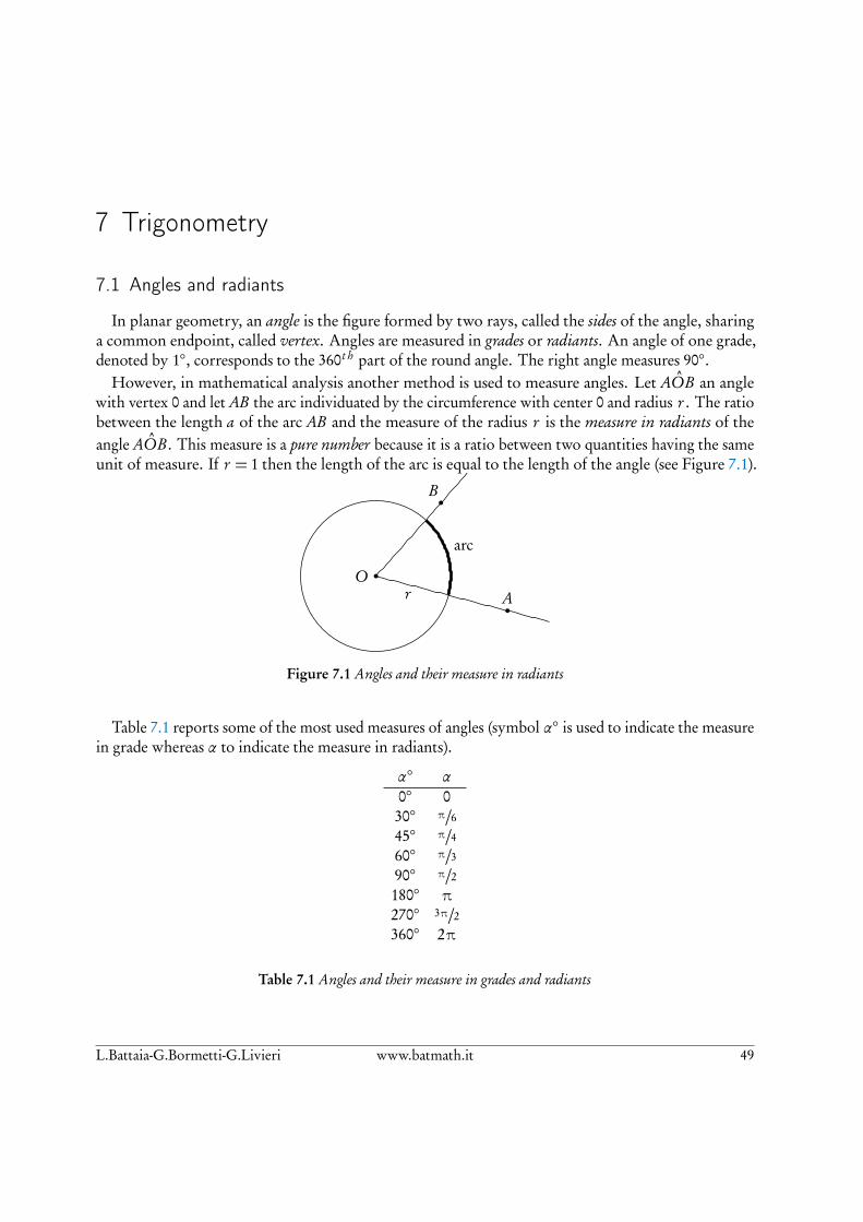
In planar geometry, an angle is the figure formed by two rays, called the sides of the angle, sharinga common endpoint, called vertex. Angles are measured in grades or radiants. An angle of one grade,denoted by 1�, corresponds to the 360t h part of the round angle. The right angle measures 90�.
However, in mathematical analysis another method is used to measure angles. Let AOB an anglewith vertex 0 and let AB the arc individuated by the circumference with center 0 and radius r . The ratiobetween the length a of the arc AB and the measure of the radius r is the measure in radiants of theangle AOB . This measure is a pure number because it is a ratio between two quantities having the sameunit of measure. If r = 1 then the length of the arc is equal to the length of the angle (see Figure 7.1).
OA
B
arc
r
Figure 7.1 Angles and their measure in radiants
Table 7.1 reports some of the most used measures of angles (symbol ↵� is used to indicate the measurein grade whereas ↵ to indicate the measure in radiants).
↵� ↵0� 030� ⇡/645� ⇡/460� ⇡/390� ⇡/2180� ⇡270� 3⇡/2360� 2⇡
Table 7.1 Angles and their measure in grades and radiants
L.Battaia-G.Bormetti-G.Livieri www.batmath.it 49

7 Trigonometry Precalculus
Although the definition of the measurement of an angle does not support the concept of negative angle,in applications, it is frequently useful to impose a convention that allows positive and negative angularvalues, to represent orientations and/or rotations in opposite directions relative to some reference. Apositive sign is attributed to angles oriented anti-clockwise and negative to angles oriented clockwise.There exists a direct correspondence between circumference arcs and angles. To measure an angle onemoves (clockwise or anti-clock-wise) from the point of intersection between the circumference and thefirst side to the point of intersection between the circumference and the second side. In particular, it ispossible to “travel” the circumference more than one time, obtaining angles “larger” than 2⇡. Theseangles are named generalized angles.For example, with reference to Figure 7.2, you can imagine to start from the point P and “travel” thearc (of length 1) to join the point Q. At this point, you continue along the circumference to reach againthe point Q. In this case the length of the “journey” will be 2⇡+ 1.
O
A
B
arc
P
Q
r = 1
Figure 7.2 Generalized angles
When working with a Cartesian plane, it is always possible to assume that the vertex of the anglecoincides with the origin and the first side with the positive semi-positive x-axis. In this situation, tomeasure angles, it is necessary to draw the circumference described by equation x2 + y2 = 1. Thiscircumference, with unit radius, is named geometric circumference. At this point, angles are identifiedwith the arcs of this circumference. Moreover, it is possible to associate with any real number a pointon the circumference (this association is not unique because of the definition of generalized angles), by“travelling” the circumference (clockwise or anti-clockwise), starting from the point (0,1), for an arc oflength the absolute value of the real number.
7.2 Sine and cosine functions
Le P = (xP , yP ) the point on the geometric circumference associated with the real number x. Theabscissa, xP , and the ordinate, yP , of P have a great impact on applications. In particular, the followingdefinition holds.
Definition 7.1. The abscissa of the point P is named cosine of the real number x; the ordinate of the pointP is named sine of the real number x. Precisely:
(7.1) xP = cos(x), yP = sin(x), or, simplyxP = cos x, yP = sin x.
50 www.batmath.it L.Battaia-G.Bormetti-G.Livieri

Precalculus 7.2 Sine and cosine functions
Figures 7.3 and 7.4 represent the functions introduced above.
1
−1
1 2 3 4 5 6 7 8 9−1−2−3
Figure 7.3 The cosine function
1
−1
1 2 3 4 5 6 7 8 9−1−2−3
Figure 7.4 The sine function
Both sine and cosine functions (hereafter trigonometric functions) are periodic. In mathematics, a periodicfunction is a function that repeats its values in regular intervals or periods. Trigonometric functionsrepeat over intervals of 2⇡. Periodic functions are used throughout science to describe oscillations,waves, and other phenomena that exhibit periodicity. Any function which is not periodic is calledaperiodic. Figure 7.5 represents a function obtained by opportunely mixing trigonometric functions.
1
2
3
4
−1
−2
−3
1 2 3 4 5 6 7 8 9 10 11 12 13−1
Figure 7.5 Oscillatory function
L.Battaia-G.Bormetti-G.Livieri www.batmath.it 51

7 Trigonometry Precalculus
7.3 Addition formulae
In this section some important formulae linked to trigonometric functions are given. In particular,the sum and difference formulae.
(7.2) cos(x ± y) = cos x cos y ⌥ sin x sin y, sin(x ± y) = sin x cos y ± cos x sin y .
For instance, from
cos⇡
4=p
22
, sin⇡
4=p
22
, cos⇡
6=p
32
, sin⇡
6=
12
,
one obtains
cos⇣⇡
4� ⇡
6
⌘= cos
⇡
4cos⇡
6+ sin
⇡
4sin⇡
6=p
22
p3
2+p
22
12=p
6+p
24
.
In particular, setting x = y:
(7.3) cos(2x) = cos2 x � sin2 x , sin(2x) = 2sin x cos x .
52 www.batmath.it L.Battaia-G.Bormetti-G.Livieri

9 Inverse trigonometric functions. 39
9 Inverse trigonometric functions.
The sine and cosine function cannot be inverted on the entire real line, however we can find an
inverse by restricting the dominion of the function. So consider the “restricted functions”
cos ∶ [0, π]→ [−1,1] , sin ∶ [−π2,π
2]→ [−1,1] .
With this restriction the cosine is a strictly decreasing function and the sine is a strictly increasing
function, so it is possible to define the inverse functions
arccos ∶ [−1,1]→ [0, π] , arcsin ∶ [−1,1]→ [−π2,π
2] .
Fig. 6: Red: graph of the arcsin, blue: graph of the arccos.
Equivalently, the sin and cos function can be defined, by looking at the triangle in Figure 7, as
● sin (x) = ah .
● cos (x) = bh
Hence, by looking at Figure 8 we get that, the so-called secant function is such that

9 Inverse trigonometric functions. 40
Fig. 7: Trigonometric triangle.
secant (θ) ⋅ cos (θ) = 1⇒ secant (θ) = 1
cos (θ)
and, finally, the tangent, as defined in Figure 8, must be such that
secant (θ) ⋅ sin (θ) = tan (θ)⇒ tan (θ) = sin (θ)cos (θ)
.

9 Inverse trigonometric functions. 41
Fig. 8: Sine, cosine and the tangent.

10 Principle of Induction 42
10 Principle of Induction
Axiom 1. ∀ proposition Pn defined on the set of integer number N:
[Pn∗ ∧ (∀n > n∗ ∶ Pn ⇒ Pn+1)]⇒ (∀n > n∗ ∶ Pn)
Esercize 1. Compute the sum of the first n integer as a function of n.
Sn = 1 + 2 + ... + n.
Therefore:
S1 = 1
S2 = 1 + 2 = 3 = (2 ⋅ 3)/2
S3 = 1 + 2 + 3 = 6 = (3 ⋅ 4)/2
S4 = 1 + 2 + 3 + 4 = 10 = (4 ⋅ 5)/2
Guess: Sn = n ⋅ (n + 1)/2. Let’s show it by induction.
● S1 = 1⇒ true.
● Assume Sn = n ⋅ (n + 1)/2. Compute:
Sn+1 = Sn + n + 1 = n ⋅ (n + 1)2
+ n + 1 = (n + 1) [n2+ 1] = (n + 1) ⋅ (n + 2)
2.⇒ ok!
Esercize 2. Show that:
(1 + x)n ≥ 1 + nx,x ≥ −1, n ∈ N.
● (1 + x)0 = 1 ≥ 1⇒ ok!.
● Assume (1 + x)n ≥ 1 + nx and compute:
(1 + x)n+1 = (1 + x) (1 + x)n ≥
≥ (1 + x) (1 + nx) = 1 + nx + x + nx2 =
= 1 + (n + 1) x + nx2 ≥ 1 + (n + 1) x⇒ ok!
For all n ∈ N we define
n! = n (n − 1) (n − 2)⋯1.

10 Principle of Induction 43
Moreover we define for any couple of integers
(nk) = n!
k! (n − k)!.
With this definition the following properties hold
( n
k + 1) + (n
k) = (n + 1
k + 1)
(n0) = (n + 1
0) = 1
(nn) = (n + 1
n + 1) = 1
Esercize 3. Show that:
(a + b)n =n
∑k=0
(nk) an−k bk,
where:
(nk) = n!
k! (n − k)!
● For n = 1 we get:
(a + b)1 =1
∑k=0
(1
k) an−k bk = (1
0) a + (1
1) b = a + b⇒ ok!
● Assume (a + b)n = ∑nk=0 (nk) an−k bk Compute:
(a + b)n+1 = (a + b)n
∑k=0
(nk) an−k bk =
n
∑k=0
(nk) an−k+1 bk +
n
∑k=0
(nk) an−k bk+1
The first term is:
n
∑k=0
(nk) an−k+1 bk = (n
0) an+1 +
n
∑k=1
(nk) an−k+1 bk q=k−1= (n
0) an+1 +
n−1
∑q=0
( n
q + 1) an−q bq+1
k=q= (n0) an+1 +
n−1
∑k=0
( n
k + 1) an−k bk+1.
The second term is:
n
∑k=0
(nk) an−k bk+1 =
n−1
∑k=0
(nk) an−k bk+1 + (n
n) bn+1
Then:
(a + b)n+1 = (n0) an+1 +
n−1
∑k=0
( n
k + 1) an−k bk+1 +
n−1
∑k=0
(nk) an−k bk+1 + (n
n) bn+1
= (n0) an+1 +
n−1
∑k=0
[( n
k + 1) + (n
k)] an−k bk+1 + (n
n) bn+1

11 Sequences 44
Remember that:
( n
k + 1) + (n
k) = (n + 1
k + 1)
(n0) = (n + 1
0) = 1
(nn) = (n + 1
n + 1) = 1
Thus:
(a + b)n+1 = (n0) an+1 +
n−1
∑k=0
( n
k + 1) an−k bk+1 +
n−1
∑k=0
(nk) an−k bk+1 + (n
n) bn+1
= (n0) an+1 +
n−1
∑k=0
[( n
k + 1) + (n
k)] an−k bk+1 + (n
n) bn+1
= (n0) an+1 +
n−1
∑k=0
(n + 1
k + 1) an−k bk+1 + (n
n) bn+1
k+1→q=k= (n0) an+1 +
n
∑k=1
(n + 1
k) an−k+1 bk + (n
n) bn+1
= (n + 1
0) an+1 +
n
∑k=1
(n + 1
k) an−k+1 bk + (n + 1
n + 1) bn+1
=n+1
∑k=0
(n + 1
k) an−k+1 bk ⇒ ok!
11 Sequences
Definition 21. A sequence is any application:
s ∶ E ⊂ N→ R,
from a subset of N to R. We indicate usually the image of a natural number sub s as:
s (n) = sn.
Definition 22. A sequence pn is said to converge if there exists a real number p ∈ R such that:
∀ε > 0∃nε ∈ N ∶ ∀n ≥ nε ⇒ ∣pn − p∣ < ε.
In this case we write:
pn → p or limn→∞
pn = p.
We add also the two following definitions:
∀M > 0∃nε ∈ N ∶ ∀n ≥ nε ⇒ pn >M,
and
∀M > 0∃nε ∈ N ∶ ∀n ≥ nε ⇒ pn < −M,

11 Sequences 45
and we write, respectively, that:
pn → ±∞ or limn→∞
pn = ±∞.
and we say that the sequence is divergent. If the sequence does not diverge or converge we say that
it has no limit.
Theorem 11.1. Suppose that (pn) is a sequence. If it exists the limit ` = limn→∞ pn then this limit
is unique.
Proof. Suppose that there exist two distinct limits ` and `′. Hence it must happen that
∀ε > 0∃nε ∈ N ∶ ∀n ≥ nε ⇒ ∣pn − `∣ < ε.
∀ε > 0∃mε ∈ N ∶ ∀m ≥ mε ⇒ ∣pm − `′∣ < ε.
Hence, for an arbitrary small ε > 0 take any integer k ≥ max (snε, smε) and consider
∣` − `′∣ ≤ ∣` − pk∣ + ∣pk − `′∣ < 2 ε.
Since ε is arbitrary small we get ` = `′.
The following theorem clarify why a limit point is called a limit point:
Theorem 11.2. If p is a limit point (accumulation point) of E ⊂ R then there exists a sequence
pn ∈ E such that pn → p.
For all n ∈ N we known that there exists a point pn in E such that:
∣p − pn∣ <1
n.
Now for all ε > 0 take n > 1ε , therefore for all n ≥ n > 1
ε we have that:
∣p − pn∣ <1
n≤ 1
n< ε,
which is our statement.
Esercize 4. Show that ∀a, b ∈ R:
∣a − b∣ ≥ ∣∣a∣ − ∣b∣∣ , ∀a, b ∈ R..
(Reverse Triangular Inequality).
Let’s write:
a = a − b + b = (a − b) + b.

11 Sequences 46
Therefore:
∣a∣ = ∣(a − b) + b∣ ≤ ∣a − b∣ + ∣b∣ ,⇒ ∣a∣ − ∣b∣ ≤ ∣a − b∣ (11.1)
where we have used the triangular inequality. Now exchange a with b:
∣b∣ = ∣(b − a) + a∣ ≤ ∣b − a∣ + ∣a∣⇒ ∣b∣ − ∣a∣ ≤ ∣b − a∣ . (11.2)
Equations (11.1)-(11.2) imply that:
∣∣a∣ − ∣b∣∣ ≤ ∣a − b∣ . (11.3)
Definition 23. Suppose that P (n) is a proposition on N. Instead of saying
∃sn ∶ ∀n ≥ sn⇒ P (n) ,
we will say that P (n) holds for n “sufficiently large”.
Esercize 5. Prove that if sn → p then ∣sn∣→ q = ∣p∣. Is the converse true?
We know that:
∀ ε > 0 ∃ n > 0 ∶ ∀ n > n→ ∣pn − p∣ < ε (11.4)
The quantity ∣∣pn∣ − ∣p∣∣ can be maximized using the reverse triangular inequality by:
∣∣pn∣ − ∣p∣∣ ≤ ∣pn − p∣ (11.5)
Then we have that:
∀ ε > 0 ∃ n > 0 s.c. ∀ n > n→ ∣∣pn∣ − ∣p∣∣ ≤ ∣pn − p∣ < ε, (11.6)
which is the thesys. The converse is not true. Take sn = (−1)n ⇒ ∣sn∣ = 1 → 1, nevertheless sn
doesn’t converge.
Theorem 11.3. Let pn be a sequence such that is it exists p = limn→∞ pn. Therefore pn is bounded,
in the sense that pn ∈ Nρ (p) for all n.
Proof. Consider the definition of limit of a sequence and take ε = 1. Hence there exists N such that
for all n > N we have ∣pn − p∣ < 1 that is pn ∈ N1 (p). Now consider any number ρ such that
ρ ≥ max (∣p1 − p∣ , ∣p2 − p∣ , ∣p3 − p∣ , ..., ∣pN−1 − p∣ ,1)
hence pn ∈ Nρ (p) for all n.
Theorem 11.4. Suppose sn and tn are two sequences in R and assume further than sn → s and
tn → t, thus:

11 Sequences 47
1. (sn + tn)→ s + t.
2. (sn tn)→ s t.
3. (c + sn)→ c + s and (c sn)→ c s for any number c.
4. if sn → s and s ≠ 0 then for n sufficiently large we have sn ≠ 0 and moreover we have 1sn→ 1
s .
Proof.
1. Take an arbitrary small ε > 0. Since both pn and tn converge then there will be two integers
n1,ε and n2,ε such that for all n ≥ n1,ε we have ∣sn − s∣ < ε2 and for all n ≥ n2,ε we have
∣tn − t∣ < ε2 . Hence for all n ≥ max (n1,ε, n2,ε) we get
∣sn + tn − (s + t)∣ = ∣sn − s + tn − t∣ ≤ ∣sn − s∣ + ∣tn − t∣ <ε
2+ ε
2= ε.
2. We want to evaluate the difference
∣sn tn − s t∣ = ∣sn tn − sn t + sn t − s t∣ = ∣sn (tn − t) + t (sn − s)∣ ≤ ∣sn∣ ∣tn − t∣ + ∣t∣ ∣sn − s∣
Since sn → s we know that sn is limited that is there exists A ≥ 0 such that ∣sn∣ ≤ A for all n.
Let’s assume that A > 0 since the case A = 0 (which implies sn = 0 for all n) is trivial. Besides
we know that, for all ε there exist n1,ε and n2,ε such that for all n ≥ n1,ε we have ∣sn − s∣ < ελ
and for all n ≥ n2,ε we have ∣tn − t∣ < ελ , where λ > 0 is to be chosen, whence
∣sn tn − s t∣ ≤ ∣A∣ ∣tn − t∣ + ∣t∣ ∣sn − s∣ < Aε
λ+ ∣t∣ ε
λ,
If now we choose λ such that
Aε
λ+ ∣t∣ ε
λ= ε⇔ λ = A + ∣t∣ .
we get that for all ε > 0 there exists snε = max (n1,ε, n2,ε) such that for all n ≥ snε we get
∣sn tn − s t∣ < ε.
3. Immediate form 2) and 3) since the constant sequence cn = c converges to c.
4. We know that for all ε > 0 there exists a snε such that ∀n ≥ snε we have ∣sn − s∣ < ε. Since
s ≠ 0 it cannot happen that definitively sn = 0 otherwise we will get ∣s∣ < ε which is impossible
since s ≠ 0. Hence there must exists a constant c > 0 such that ∣sn∣ ≥ c for n sufficiently large.
Whence, for n sufficiently large, we have
∣ 1
sn− 1
s∣ = ∣s − sn∣
s sn≤ ∣s − sn∣
s c< ε
s c
hence 1sn→ 1
s . ✠

11 Sequences 48
Esercize 6. Let pn be a sequence in R such that pn → p and pn ≥ 0 for all n. Prove that
1. p ≥ 0.
2. p12n → p
12
1) Suppose by contradiction that p < 0. Then there exists ε > 0 such that p + ε < 0 and for n
sufficiently large we have ∣pn − p∣ < ε which is equivalent to −ε < pn − p < ε which is equivalent to
p − ε < pn < p + ε < 0
which is impossible since pn ≥ 0 for all n.
2) Let’s distinguish two cases. If p = 0 then for n sufficiently large
pn < ε2
hence p12n < ε, whence p
12n → 0.
If p > 0 then
∣√pn −√p∣ = ∣√pn −
√p∣
∣√pn +√p∣
∣√pn +√p∣
= ∣pn − p∣√pn +
√p< ∣pn − p∣√
p<ε√p
√p
= ε
Esercize 7. Compute limn→∞
√n2 + n − n.
We first note that:√n2 + n →∞ and of course n →∞. The idea is that for large n the quantity
n2+n is dominated by n2 and therefore the limit under study should be finite. Let’s try to rationalize
the sequence:
√n2 + n − n =
(√n2 + n − n) (
√n2 + n + n)
√n2 + n + n
= n2 + n − n2√n2 + n + n
= n√n2 + n + n
= n
n (√
1 + 1n + 1)
= 1
(√
1 + 1n + 1)
→ 1
2. (11.7)
Theorem 11.5. The following two assertions hold:
1. Let xn and yn be two convergent sequences in R. Assume that xn ≤ yn for n sufficiently large.
Hence limn xn ≤ limn yn

11 Sequences 49
2. Let xn, yn and zn be three sequences in R. Suppose that xn ≤ yn ≤ zn for n sufficiently large
and that limn xn = limn zn = a. Hence there exists limn yn and it is equal to a.
Proof. The 1) is trivial. Let’s prove assertion 2). We know that for all ε > 0 there exists n1 and
n2 such that for all n ≥ n1 we have ∣xn − a∣ < ε and for all n ≥ n2 we have ∣zn − a∣ < ε. Hence if
n ≥ max (n1, n2) we have
a − ε < xn ≤ yn ≤ zn < a + ε,
whence the thesis. ✠
A notable limit.
We want to compute:
limn→∞
n sin( 1
n) = 0 ⋅ ∞.
Consider a unit circle and an angle x ∈ (0, π2 ).
The length of the arc AC is AC = 1×x = x, the length of the segment CD is sin (x) while the length
OD = cos (x). Now is clear that the area of the triangle OAC = 1×sin(x)2 is less than the area of the
circular sector OAC which is 12 12 x = x
2 which is less than the area of the triangle OAB which is1×tan(x)
2 = 12 tan (x) or in formula:
0 ≤ 1
2sin (x) ≤ 1
2x ≤ 1
2tan (x)⇒ 0 ≤ sin (x) ≤ x ≤ tan (x) .
or graphically:
For x = 1n we have:
0 ≤ sin( 1
n) ≤ 1
n≤ tan( 1
n) =
sin ( 1n)
cos ( 1n),

11 Sequences 50
i.e.,
1
sin ( 1n)≥ n ≥
cos ( 1n)
sin ( 1n)⇒
1 ≥ sin( 1
n) n ≥ cos( 1
n) ≥ 0⇒
0 ≤ cos( 1
n) ≤ n sin( 1
n) ≤ 1.
Nevertheless:
cos( 1
n)→ 1.
Thus:
limn→∞
n sin( 1
n) = 1.
11.1 Monotonicity
Definition 24. A sequence sn of real numbers is said to be:
● monotonically increasing if sn ≤ sn+1.
● monotonically decreasing if sn ≥ sn+1.
Theorem 11.6. Every increasing (respectively decreasing) sequence sn converges to
limn→∞
sn = sup{sn∣n ∈ N} (respectively limn→∞
sn = inf {sn∣n ∈ N} ).

11 Sequences 51
Proof. Suppose sn is increasing and let ` = sup{sn∣n ∈ N}. If ` = ∞ then sn is not bounded and
hence ∀M > 0 I can find snM such that for n ≥ snM we have sn >M (otherwise it would be bounded
from above), whence sn →∞. Suppose now that ` <∞. By the definition of supremum we know
that sn ≤ ` for all n and that for all ε > 0 the exist snε such that ` − ε < ssnε . Since sn is increasing
then for all n ≥ snε we have
` − ε < ssnε ≤ sn ≤ ` < ` + ε,
whence ∣sn − `∣ < ε, i.e. sn → ` and a similar reasoning applies for the decreasing sequences. ✠
Corollario 11.7. Suppose that sn is a monotonically increasing (resp. decreasing) sequence. Hence
sn converges to a finite limit if and only if it is bounded from above (resp. below).
Proof. Let’s prove before implication ⇒. If sn is increasing and it converges to a finite limit
therefore for the Theorem 11.6 we must have supn sn <∞ otherwise we would have sn →∞ which
is impossible. Hence sn is bounded from above.
Let’s prove now implication ⇐. Since sn is bounded from above we know that exists and it is finite
the supremum ` = supn sn. By the theorem 11.6 we know that sn → `.✠
11.2 Subsequences
Definition 25. Given a sequence sn and a second sequence of strictly increasing positive integers
n1 < n2 < ... < nk < ... we call the sequence snk a sub-sequence of sn. If snk converges its limit is
called a subsequential limit of sn. In particular note that it must happens that nk ≥ k.
Theorem 11.8. A sequence sn converges to s in and only if every subsequence of sn converges to s.
Proof.
The implication ⇐ is trivial. If every subsequence converges to s hence since sn is a subsequence of
itself it converges to s.
Let’s now consider the other implication ⇒. Suppose that sn → s. Let U be a neighborhood of s.
Then there exists N such that for all n ≥ N it happens that sn ∈ U . Since nk ≥ k therefore if k ≥ Nwe get nk ≥ k ≥ N and hence snk ∈ U , whence snk → s. ✠
Exercizes.
● Show that sn = (−1)n has no limit.
Solution. Since s2n = 1→ 1 and s2n+1 = −1→ −1 the sequence has no limit.

11 Sequences 52
● Prove that sn = loga (n) with a > 1 is such that sn →∞.
Solution. Consider an M > 0. We want to find a nM such that for all n ≥ nM it holds
loga (n) ≥M.
Since loga with a > 1 is an increasing function it is enough to consider take any nM such that
nM ≥ aM .
So now consider a generic n with n ≥ nM ≥ aM , then by the monotonicity of the logarithm we
get
loga (n) ≥ loga (nM) ≥ loga (aM) =M.
● Find the limit of the sequence sn = 3 − 1log2(n)
.
Solution. The guess is that the limit is 3. Let ε > 0 be arbitrarily small. The condition
∣sn − 3∣ < ε
is equivalent to
∣ 1
log2 (n)∣ < ε.
Since n ≥ 1 we get1
log2 (n)< ε.
So it is enough to take any nε such that nε > 21/ε.
11.3 Some Notable Limits
● Let a ∈ R with a ≠ 1. Then
limn→∞
an =
⎧⎪⎪⎪⎪⎪⎨⎪⎪⎪⎪⎪⎩
0 if ∣a∣ < 1
∞ if a > 1
∄ if a ≤ −1
Case ∣a∣ < 1. Hence ∣a∣ = 11+h for some h > 0. By the binomial inequality
(1 + h)n ≥ 1 + nh ≥ nh
whence
0 ≤ 1
(1 + h)n≤ 1
nh
the results follows from the fact that 1n → 0.
Case a > 1. Hence a = 1 + h for some h > 0. Therefore

11 Sequences 53
an = (1 + h)n ≥ 1 + nh.
Since n→∞ and h > 0 we have the result.
Suppose that a = −1. Let sn = (−1)n. Therefore I can define two subsequences s2n = 1 → 1
and s2n+1 = −1→ −1, hence sn does not converge.
Finally, suppose a < −1, whence a = − ∣a∣ with ∣a∣ > 1. Hence an = (−1)n ∣a∣n with ∣a∣n → ∞.
Let sn = an. As a consequence s2k →∞ and s2k+1 → −∞ hence sn does not converge.
● Let a ∈ R be such that a > 1 and let k be an integer number k ≥ 1. We want to compute
limn→∞
nk
an.
Write a = 1 + h. For n sufficiently large we will have n > k + 1 hence
an = (1 + h)n =n
∑m=0
( nm
)hm ≥ ( n
k + 1)hk+1 = n (n − 1)⋯ (n − k)
(k + 1)!hk+1,
whence
0 ≤ nk
an≤ (k + 1) nk
hk+1 n (n − 1) ⋯ (n − k)´¹¹¹¹¹¹¹¹¹¹¹¹¹¹¹¹¹¹¹¹¹¹¹¹¹¹¹¹¹¹¹¹¹¹¹¹¹¹¹¹¹¹¹¹¹¹¹¹¹¹¹¹¹¹¸¹¹¹¹¹¹¹¹¹¹¹¹¹¹¹¹¹¹¹¹¹¹¹¹¹¹¹¹¹¹¹¹¹¹¹¹¹¹¹¹¹¹¹¹¹¹¹¹¹¹¹¹¹¹
k+1 terms
= (k + 1)hk+1 n (1 − 1
n) ⋯ (1 − k
n)→ 0.
● Find a formula for the sum the first n-powers of any real number x
Sn = 1 + x + x2 + ... + xn
We multiply both side of the equation by 1 − x obtaining
(1 − x) Sn = (1 + x) (1 + x + x2 + ... + xn)
= 1 + x + x2 + ... + xn − x (1 + x + x2 + ... + xn)
= 1 + x + x2 + ... + xn − x − x2 − ... − xn+1
= 1 − xn+1,
whence
Sn =1 − xn+1
1 − x.
As a consequence, by looking backward in the section dedicated to the notable limits, we can
claim that
limn→∞
Sn =
⎧⎪⎪⎪⎪⎪⎨⎪⎪⎪⎪⎪⎩
11−x if ∣x∣ < 1,
+∞ if x ≥ 1,
∄ if x ≤ −1.

11 Sequences 54
● We want to compute
limnn1/n.
It is immediate to see that for all n ≥ 1 then n1/n ≥ 1 since the inequality n1/n < 1 would lead
to
n1/n⋯n1/n´¹¹¹¹¹¹¹¹¹¹¹¹¹¹¹¹¹¹¹¹¹¹¸¹¹¹¹¹¹¹¹¹¹¹¹¹¹¹¹¹¹¹¹¹¹
n times
< 1⋯1 = 1,
nevertheless n1/n⋯n1/n´¹¹¹¹¹¹¹¹¹¹¹¹¹¹¹¹¹¹¹¹¹¹¸¹¹¹¹¹¹¹¹¹¹¹¹¹¹¹¹¹¹¹¹¹¹
n times
= n which is impossible. Hence n1/n = 1 + an with an ≥ 0 that is
(1 + an)n = n. Now we have
n = (1 + an)n = 1 + (n1)an + (n
2)a2n + ... ≥ 1 + (n
2)a2n = 1 + n (n − 1)
2a2n.
The inequality 1 + n (n−1)2 a2n ≤ n re-arranged gives
0 ≤ a2n ≤2
n→ 0.
Hence an → 0 and thus n1/n → 1.
● We want to compute
limn→∞
nn
n!
Consider thatnn
n!= n ⋅ n⋯nn ⋅ (n − 1)⋯1
= n
n®=1
⋅ n
n − 1²
>1
⋯ n
2®>1
⋅n > n
hence
limn→∞
nn
n!=∞
or
limn→∞
n!
nn= 0
● For a > 1 compute the limit of the sequence sn = loga(n)n .
Consider that sn = loga (n1n ) but n
1n → 1 hence sn → loga (1) = 0.
More generally for a > 1 and b > 0 we have
limn→∞
loga n
nb= 0.
● Let a > 1. We want to compute the limit
limn→∞
an
n!.
Let xn = an
n! . Consider that

11 Sequences 55
xn+1xn
= an+1
(n + 1)!n!
an= aa
n
ann!
(n + 1)n!= a
n + 1→ 0
which means that
∀ε > 0,∃nε ∶ ∀n ≥ nε ⇒ ∣xn+1xn
∣ < ε.
In particular, there exists ε ∈ (0,1) and an N such that for all n > N we have
0 < xn+1xn
< ε⇒ 0 < xn+1 < εxn, (11.8)
where we also have used the fact that xn ≥ 0 for all n. By iteration of the (11.8) we get
0 < xn+1 < εxn < ε2 xn−1 < ε3 xn−2 < ... < εn−N xN+1.
Consider now that N is a fixed given number, hence we can let n →∞ obtaining εn−N → 0
then
limn→∞
an
n!= 0
so the factorial grows faster than the exponential.
Orders of Infinity.
Suppose that an →∞ and bn →∞. We say that an ≪ bn if bnan→∞, that is both an and bn diverge,
however bn diverges faster than an. Summing up the results of the limits above we can say that, for
all a > 1 and b > 0, that the following orders of infinity hold:
loga (n) ≪ nb ≪ an ≪ n! ≪ nn.
Definition 26. We say that an ∼ bn for n→∞ if:
limn→∞
anbn
= 1.
In this case we also say that an and bn are asymptotically equivalent. For example if an → L then
an ∼ L.
Observation 1. The following properties hold:
● If an ∼ bn and bn → l ∈ R ∪ {±∞} then an → l.

11 Sequences 56
● If an ∼ bn and bn ∼ cn then an ∼ cn.
● If an ∼ bn then for every sequence cn such that cn ≠ 0∀n we have:
an cn ∼ bn cn,ancn
∼ bncn,cnan
∼ cnbn. (11.9)
Proof. We prove just the case bn → ` with ` a finite number and ` > 0. Since an ∼ bn we have
for sufficiently large n
1 − ε < anbn
< 1 + ε,
or
bn (1 − ε) < an < bn (1 + ε)
Now if ε → 0 then n → ∞ and so bn → ` which implies, by the comparison theorem, that
an → `.
Consider for example n√
1 + 1n +
1n2 ∼ n.
Esercize 8. Compute:
limn→∞
n√n − n2
n + 1.
Note that:
n√n − n2 = n
32 − n2 ∼ −n2 because
3
2< 2,
moreover:
n + 1 ∼ n.
Threrfore we have:n√n − n2
n + 1∼ −n2
n= −n→ −∞. (11.10)
Esercize 9. Show that:
limn→∞
p1n = 1,∀ p > 0 (11.11)
Assume p ≥ 1. Consider xn = p1n − 1, thus xn ≥ 0 and:
(1 + xn)n = p.

11 Sequences 57
Using binomial inequality:
(1 + xn)n ≥ 1 + nxn ⇒
p ≥ 1 + nxn ⇒
0 ≤ xn ≤ p − 1
n⇒
xn → 0⇒
p1n → 1.
If 0 < p < 1 then consider q = 1p > 1. Therefore q
1n → 1 and:
p1n = 1
q1n
→ 1
1= 1.
Esercize 10. Compute:
limn→∞
4n + 2n
1n2 + 5n
.
4n + 2
n∼ 4n.
1
n2+ 5n ∼ 5n.
As a consequence:
limn→∞
4n + 2n
1n2 + 5n
= limn→∞
4n
5n= 4
5.
Esercize 11. Compute:
limn→∞
n −√n + n2.
When dealing with square roots it’s wise to rationalize:
n −√n + n2 =
(n −√n + n2) (n +
√n + n2)
n +√n + n2
=n2 − (n + n2)n +
√n + n2
= − n
n (1 +√
1n + 1)
→ −1
2(11.12)
Esercize 12. Compute:
limn→∞
(3n + 4n)1n .
(3n + 4n)1n = {4n [1 + (3
4)n
]}1n
= 4 [1 + (3
4)n
]1n
.
Neverthelss for 0 < p < 1, pn → 0, thus:
(3n + 4n)1n = 4 [1 + (3
4)n
]1n
→ 4. (11.13)

11 Sequences 58
The Euler Sequence
Let
an = (1 + 1
n)n
be the a sequence of real numbers (also known as the Euler sequence). First notice that, by the
binomial inequality, we have
an ≥ 1 + n 1
n= 2.
Using the binomial theorem we get
an =n
∑k=0
(nk)( 1
n)k
= 1 +n
∑k=1
(nk)( 1
n)k
= 1 +n
∑k=1
n (n − 1) ⋯ (n − k + 1)nk
1
k!
= 1 + 1 +n
∑k=2
n (n − 1) ⋯ (n − k + 1)nk
1
k!
= 2 +n
∑k=2
[1 ⋅ (1 − 1
n) ⋅ (1 − 2
n)⋯(1 − k − 1
n)] 1
k!
< 2 +n
∑k=2
[1 ⋅ (1 − 1
n + 1) ⋅ (1 − 2
n + 1)⋯(1 − k − 1
n + 1)] 1
k!
< 2 +n+1
∑k=2
[1 ⋅ (1 − 1
n + 1) ⋅ (1 − 2
n + 1)⋯(1 − k − 1
n + 1)] 1
k!= an+1. (11.14)
Now we show that the sequence is bounded from above. Note that
k! = 1 2 3⋯k ≥ 1 2 2⋯2 = 2k−1,
whence
2 < an = 1 +n
∑k=1
⎡⎢⎢⎢⎢⎢⎢⎢⎣
1 ⋅ (1 − 1
n)
´¹¹¹¹¹¹¹¹¹¹¹¸¹¹¹¹¹¹¹¹¹¹¹¶<1
⋅(1 − 2
n)
´¹¹¹¹¹¹¹¹¹¹¹¸¹¹¹¹¹¹¹¹¹¹¹¶<1
⋯(1 − k − 1
n)
´¹¹¹¹¹¹¹¹¹¹¹¹¹¹¹¹¹¹¹¹¹¹¹¹¸¹¹¹¹¹¹¹¹¹¹¹¹¹¹¹¹¹¹¹¹¹¹¹¹¶<1
⎤⎥⎥⎥⎥⎥⎥⎥⎦
1
k!
< 1 +n
∑k=1
1
k!≤ 1 +
n
∑k=1
1
2k−1= 1 + 2
n
∑k=1
1
2k< 1 + 2 lim
n→∞
n
∑k=1
1
2k= 1 + 2 ( 1
1 − 12
− 1) = 3.
Hence ∃e = limn→∞ (1 + 1n)n and 2 < e ≤ 3.
Exercise. Compute the limit of the sequence sn = (1 + 5n2 )
n2
.

11 Sequences 59
Solution. Call m = n√5, hence
limn→∞
(1 + 5
n2)n2
= limm→∞
(1 + 1
m2)5m2
= limm→∞
((1 + 1
m2)m2
)5
Call k =m2, hence
limm→∞
((1 + 1
m2)m2
)5
= limk→∞
((1 + 1
k)k
)5
= e5.
So that
sn → e5.
Economic Application
Suppose that, at time n, the price of a good is pn. Suppose further that the demand, for a given
price, is given by D (pn) = −b pn + a while the supply is given by S (pn) = s pn −m. Assume that the
price evolves according to
pn+1 = pn + (D (pn) − S (pn)) ,
We want to study the limit limn→∞ pn.
pn+1 = pn + (D (pn) − S (pn)) = pn + a − b pn +m − s pn ⇒
pn+1 = a +m + (1 − b − s)pn ⇒
pn+1 = α + β pn ⇒
p1 = α + β p0 ⇒
p2 = α + β α + β2 p0 ⇒
p3 = α + β α + β2 α + β3 p0 ⇒
⋮ ⋮
pn = α (1 + β + β2 +⋯ + βn−1) + βn p0 ⇒
pn = α (1 − βn
1 − β) + βn p0.

11 Sequences 60
Simplifying:
pn = α (1 − βn) + (1 − β) βn p01 − β
⇒
pn = α (1 − βn) + βn p0 − βn+1 p01 − β
⇒
pn = βn (p0 (1 − β) − α) + α1 − β
⇒
pn = (1 − b − s)n (p0 (b + s) − (a +m)) + a +mb + s
⇒
pn = (1 − (b + s))n (b + s) (p0 − pe) + a +mb + s
⇒
pn = (1 − (b + s))n (p0 − pe) + pe.
Now define b+ s = r, the quantity r represents the sum of the rate of decrasing demand and the rate
of increasing supply:
limn→+∞
pn =⎧⎪⎪⎨⎪⎪⎩
pe if 0 < r ≤ 1 (convergence with monotonic behaviour)
pe if 1 < r < 2 (convergence with non-monotonic behaviour)
For r ≥ 2 there is no limit.
Esercize 13. The return of an investment in a time horizon [0,1] is R, i.e. if we invest a quantity
of money M0 at time t0 = 0 we arrive at M0 (1 +R) at time tf = 1. Suppose that the quantity of
money is continuously invested, i.e. we invest money at time t0 wait for maturity at time t0 +∆t
and re-invest the original amount plus maturity at time t0 +∆t, then wait for maturity at time
t0 + 2 ∆t and so on. Compute which of the two strategies (in absence of transaction costs) is the
one with the largest return in the limit ∆t→ 0.
Solution. If we divide the interval [0,1] in two part the return is:
(1 + R2) (1 + R
2) = (1 + R
2)2
.
More generally if we continuously invest:
limn→∞
(1 + Rn)n
= eR.
Remember that the sequence an = (1 + Rn)n is increasing hence
eR = limn→∞
an ≥ a1 = 1 +R.
Therefore (as expected) continuously investing is the winning strategy. In practice transaction costs
make this choice unfeasible.

11 Sequences 61
Esercize 14. Let k > 1 be a given integer. Establish if the sequence
xn =⎛⎝k sin( 1
n2) + 1
kcosn
⎞⎠
n
.
has a limit or note and in the affermative case compute it.
Solution. We know that for 0 < x < π2 then 0 < sin (x) < x and 0 < cosx < 1, hence
∣xn∣ ≤⎛⎝k
n2+ 1
k
⎞⎠
n
.
Since k > 1 there exists a δ with 0 < δ < 1 such that, for n sufficiently large
k
n2+ 1
k≤ 1 − δ
whence
∣xn∣ ≤ (1 − δ)n → 0.
11.4 “Advanced” topics on sequences.
This section discusses some advanced topics on sequences. It is an optional section that can
be skipped.
Theorem 11.9. Every sequence contains a monotone subsequence.
Proof. Consider a sequence xn. We call the m-th term xm a peak if xm ≥ xn for all n ≥m. There
are two cases.
● There are infinitely many peaks. In this case I list them according to the increasing subscript
{xn1 , xn2 , ..., xnk , ...} and since they are peaks by definition it must be
xn1 ≥ xn2 ≥ ... ≥ xnk ≥ ...,
hence a monotonically decreasing sub-sequence.
● There are finitely many peaks. Again I list them according to the increasing subscript
{xm1 , xm2 , ..., xmk}. Consider n1 =mk + 1. Hence xn1 it is not a peak and therefore it must

11 Sequences 62
exist a index n2 > n1 such that xn2 > xn1 . Nevertheless since n2 > n1 >mk then xn2 it is not
a peak, hence it must exists an index n3 > n2 such that xn3 > xn2 . Iterating this we get a
monotonically increasing sub-sequence xnk .
✠
Definition 27. Let sn be a sequence and E the set defined as:
E = {x ∈ R ∪ {+∞} ∪ {−∞} ∣∃nk ∶ snk → x} ,
i.e. the collection of all limits of the subsequences of sn. We define the upper and lower limit of sn
as:
lim supn→∞
sn = supE
lim infn→∞
sn = inf E .
Theorem 11.10. It xn and yn are real sequences then
1. lim sup(−xn) = − lim inf xn and lim inf(−xn) = − lim supxn.
2. For any a > 0 lim sup(axn) = a lim sup(xn) and lim inf(axn) = a lim inf(xn).
3. Suppose that lim supxn and lim sup yn are finite then: lim sup(xn + yn) ≤ lim sup(xn) +lim sup(yn). Suppose that lim inf xn and lim inf yn are finite then: lim inf(xn+yn) ≥ lim inf xn+lim inf yn.
4. lim inf xn ≤ lim supxn where the equality holds if and only if the sequence converges and in
this case limxn = lim inf xn = lim supxn.
Proof. 1) and 2) are obvious while 4) follows from Theorem 11.8. Let’s prove assertion 3) for the
lim sup case, the other one is similar. Hence, let X = lim supxn and Y = lim sup yn. Given ε > 0
then there exist two integers n1 and n2 such that ∀n ≥ n1 we have xn <X + ε2 and ∀n ≥ n2 we have
yn < Y + ε2. Hence if n ≥ max (n1, n2) we have
xn + yn <X + Y + ε.
We can take the limn→∞ on both side of the inequality, we do not know in general if xn+yn converges,
but we know that the lim sup always exists and hence it must be
lim sup (xn + yn) ≤X + Y.✠
Theorem 11.11. Bolzano-Weiestrass Let (xn)n∈N be a sequence in R. If (xn)n∈N is bounded
then (xn)n∈N has a convergent subsequence.
Proof. According to Theorem 11.9 any sequence has a monotone-subsequence. Since (xn)n∈Nis bounded then also the monotonic sub-sequence is bounded, but then by Theorem 11.6 it is
convergent.

12 Some exercise on sequences 63
12 Some exercise on sequences
Try to solve these exercises by yourself, then look at the solutions.
Esercize 15. Let sn be the sequence defined recursively as:
s0 = a
sn+1 = 12 (sn + α
sn) ,
with a ≥ α > 0. Establish if sn converge and in this case compute its limit.
First of all notice that s0 > 0 and if sn > 0 immediately follows sn+1 > 0, hence by induction sn > 0
for all n. From the definition of the sequence we get
s2n − 2sn+1sn + α = 0
hence the second-degree polynomial has a real root whence the delta must be positive
4 s2n+1 − 4α ≥ 0
that is s2n+1 ≥ α for all n. Now consider
sn+1 − sn =1
2
s2n + αsn
− sn =s2n + α − 2 s2n
2 sn= α − s
2n
2 sn≤ 0
whence sn+1 ≤ sn, therefore the sequence is monotonically decreasing and since it is bounded from
below therefore it must exist L = limn→∞ sn. Besides every sub-sequence converge to the same limit,
hence also sn+1 → L. By the recursive rule the only possibility for L is to satisfy the equation
L = 1
2(L + α
L)⇔ L2 = 1
2(L2 + α)⇔ L2 = α
whence L = α12 .
The exercise just solved gives a rule to approximate the square root of any positive real number.
Esercize 16. Let sn be the sequence defined recursively as:
s1 =√
2
sn+1 =√
2 +√sn
Establish if sn converge and in this case compute its limit.

12 Some exercise on sequences 64
Let’s write out some terms of the sequence:
s1 =√
2
s2 =√
2 +√√
2 >√
2 = s1
Apparently the sequence seems increasing. Assume that sn+1 > sn and try to show that sn+2 > sn+1:
sn+2 =√
2 +√sn+1
(by hypothesis)>
√2 +
√sn = sn+1 ⇒ ok!
Does there exist an upper limit?
s1 =√
2 < 2
s2 =√
2 +√√
2 < 2
The last inequality is equivalent to√
2 < 4 which is more evident. Now suppose that sn < 2 and
show that sn+1 < 2:
sn+1 =√
2 +√sn <
√2 +
√2 < 2 (12.1)
The last inequality is equivalent to√
2 < 2 which is more evident. Increasing + Bounded from above
⇒:
∃ L = limn→∞
sn (12.2)
and it must satisfies:
L =√
2 +√L⇒ L4 − 4L2 −L + 4 = 0 (12.3)
Numerically:
L ≈ 1.8312....
Esercize 17. Consider: ⎧⎪⎪⎨⎪⎪⎩
a1 = 2
an+1 = 12 (an + 6)
.
Establish if an admits limit and, in this case, compute it.
Let’s write out some term of the sequence:
a1 = 2
a2 = 12 (2 + 6) = 4
a3 = 5
a4 = 112 < 11+1
2 = 6
a5 = 12(11
2 + 6) = 234 < 23+1
4 = 6
a6 = ... = 478 < 47+1
8 = 6
.

12 Some exercise on sequences 65
The induction hypothesis is that an < 6:
an+1 =1
2(an + 6) < 1
2(6 + 6) = 6.
Therefore an < 6,∀n. Is an increasing? a1 < a2. Now assume an < an+1:
an+2 =1
2(an+1 + 6) > 1
2(an + 6) = an+1.
Therefore an is limited from above and increasing ⇒
∃l ∶ limn→∞
an = l.
Note that:
limn→∞
an+1 = l.
Therefore l must verify:
l = 1
2(l + 6)⇒ l = 6⇒ lim
n→∞an = 6.
Esercize 18. Consider: ⎧⎪⎪⎨⎪⎪⎩
a1 = 1
an+1 = 3 − 1an
.
Establish if an admits limit and, in this case, compute it.
Let’s write out some term of the sequence:
a1 = 1
a2 = 3 − 1 = 2
a3 = 3 − 12 =
52 <
5+12 = 3
a4 = 3 − 25 =
135 < 13+2
5 = 3
.
The induction hypothesis is that an < 3⇒ 13 <
1an
:
an+1 = 3 − 1
an< 3 − 1
3= 8
3< 8 + 1
3= 3.
Is an increasing? a1 < a2. Now assume an < an+1:
an+2 = 3 − 1
an+1> 3 − 1
an= an+1.
Therefore an is limited from above and increasing ⇒
∃l ∶ limn→∞
an = l.
Note that:
limn→∞
an+1 = l.

12 Some exercise on sequences 66
Therefore l must verify:
l = 3 − 1
l⇒ l2 − 3 l + 1 = 0⇒ l± =
3 ±√
9 − 4
2.
Neverthelss l− = 3−√5
2 < 1 and a1 > 1 and the sequence is increasing ⇒ l− cannot be the limit of l.
Therefore:
limn→∞
an =3 +
√5
2.
Esercize 19. Find upper and lower limit of:
s1 = 0, s2m = s2m−12
, s2m+1 =1
2+ s2m.
Let’s write out some term:s1 = 0 → s2 = 0
↙s3 = 1
2 → s4 = 14 =
21−122
↙s5 = 3
4 → s6 = 38 =
22−123
↙s7 = 7
8 → s8 = 716 =
23−124
.
Similarly for the odd sequence note that:
s1 = 0, s3 =1
21, s5 =
22 − 1
22, s7 =
23 − 1
23.
Now induction implies that:
s2m = 2m−1 − 1
2m(⇒ s2m+1 =
1
2+ 2m−1 − 1
2m= 2m − 1
2m) .
Therefore:
limm→∞
s2m = limm→∞
2m−1 − 1
2m= 1
2.
limm→∞
s2m+1 = limm→∞
2m − 1
2m= 1.
Note that every subsequence can be splitted in its odd and even sub-subsequence:
↗snk
↘
s2nk+1
s2nk
Therefore it is enough to check if the odd and even sequences converge somewhere. In our case we
can conclude that:
lim sup sn = 1, lim inf sn =1
2. (12.4)
As a direct consequence sn doesn’t converge.
13 Series 67
13 Series
Definition 28. Given a sequence an, the sequence of the partial sums of an is defined as
Sn =n
∑k=1
ak.
We call the sum of the series of the an the limit, if it exists, of the partial sums and we write:
S = limn→∞
Sn =+∞
∑k=1
ak.
Observation 2. The following properties hold:
1. (Necessary condition). If
Sn =∞
∑k=0
ak <∞,
then
limk→∞
ak = 0.
The proof is immediate since an = Sn − Sn−1. So if Sn → ` for some finite ` then also Sn−1 → `
and thus an → ` − ` = 0.
2. If 0 ≤ ak ≤ ck for all k ≥ k0, with k0 given, then the convergence of ∑∞k=1 ck implies the
convergence of ∑∞k=1 ak.
3. If ak ≥ ck ≥ 0 for all k ≥ k0, with k0 given, then the divergence of ∑∞k=1 ck implies the divergence
of ∑∞k=1 ak.
The proofs of the points 2 and 3 are an application of the comparison theorem to the sequence
of partial sums Sn.
Esercize 20. For which values of x the series:
∞
∑k=0
xk,
converges?
Note that:
1 + x = (1 + x) (1 − x)1 − x
= 1 − x2
1 − x.
Therefore:
1 + x + x2 = 1 − x2
1 − x+ x2 = 1 − x2 + x2 − x3
1 − x= 1 − x3
1 − x.

13 Series 68
Iterating again:
1 + x + x2 + x3 = 1 − x3
1 − x+ x3 = 1 − x3 + x3 − x4
1 − x= 1 − x3
1 − x.
Now it’s easy to show by induction that:
1 + x + x2 + ... + xn = 1 − xn+1
1 − x.
Hence:
∞
∑k=0
xk = limn→∞
1 − xn+1
1 − x=
⎧⎪⎪⎪⎪⎪⎨⎪⎪⎪⎪⎪⎩
11−x ∣x∣ < 1
∞ x ≥ 1
no limit x ≤ −1.
13.1 Series of nonnegative terms
Theorem 13.1. Suppose that:
a1 ≥ a2 ≥ a3 ≥ ⋯ ≥ 0.
Then the series:∞
∑k=1
ak,
converges if and only if the series:∞
∑k=0
2ka2k ,
converges.
Proof.
It is immediate to see that
0 ≤∞
∑k=1
ak ≤∞
∑k=0
2k a2k ≤ 2∞
∑k=1
ak.
Concerning the first inequality note that
∑∞k=1 ak = a1 + a2 + a3 + a4 + a5 + a6 + a7 +⋯
≤ a1 + a2 + a2 + a4 + a4 + a4 + a4 +⋯= a1 + 2a2 + 4a4 +⋯= ∑∞
k=0 2k a2k
Concerning the second inequality note that
∑∞k=0 2ka2k = a1 + a2 + a2 + a4 + a4 + a4 + a4 +⋯
= a1 + a2 + a2 + a4 + a4 + a4 + a4 + a8 + a8 + a8 + a8 + a8 + a8 + a8 +⋯≤ a1 + a1 + a2 + a2 + a3 + a3 + a4 + a4 + a5 + a5 + a6 + a6 + a7 + a7 +⋯= 2 ∑∞
k=1 ak ,

13 Series 69
which completes the proof.
Observation 3. The sum+∞
∑k=0
(1
k)p
,
converges ⇔ p > 1.
We show that it doesn’t converge for p = 1:
2n
∑k=1
1
k= 1 + 1
2+ 1
3+ 1
4+ 1
5+ 1
6+ 1
7+ 1
8+⋯
> 1 + 1
2+ 1
4+ 1
4+ 1
8+ 1
8+ 1
8+ 1
8+⋯
= 1 + 1
2+ 1
2+ 1
2+⋯
= 1 + n2.
Whence
limn→∞
2n
∑k=1
1
k> limn→∞
(1 + n2) =∞.
Note that the necessary condition is verified!
More generally if p ≤ 0 the generic term is not infinitesimal and as a consequence the series diverges.
If p > 0 we can apply the 2k-criterion:
∞
∑k=1
2k1
2k p=
∞
∑k=1
(2(1−p))k,
The argument of the geometric series is < 1 if and only if:
2(1−p) < 1⇔ p > 1,
whence the thesis.
Definition 29. A series ∑∞n=1 an is said to be absolutely convergent if
∞
∑n=1
∣an∣ <∞.
Theorem 13.2. If a series is absolutely convergent then it is convergent.
Proof. Since
0 ≤ an + ∣an∣ ≤ 2 ∣an∣
we have
0 ≤m
∑n=1
(an + ∣an∣) ≤ 2m
∑n=1
∣an∣ < 2∞
∑n=1
∣an∣

13 Series 70
so the sequence sm = ∑mn=1 (an + ∣an∣) is a monotonic increasing bounded sequence and hence it must
converge. Now note that the original series
Sm =m
∑n=1
an = sm −m
∑n=1
∣an∣
is the difference of two converging sequences, hence it must converge.
13.2 Convergence Criteria for Series
1. ∑ak converges if and only if for every ε > 0 there is an integer N such that for all m ≥ n ≥ Nwe have that:
∣m
∑k=n
ak∣ ≤ ε.
2. Root test: given ∑k ak consider α = lim supn→∞ ∣an∣1n . Therefore if α < 1 the series converges,
if α > 1 the series diverges, if α = 1 the test gives no information.
Proof. We prove only the case α < 1. Assume, hence, that α = limn→∞ ∣an∣1n < 1. Therefore,
there exists an r such that, for n sufficiently large
∣an∣1/n ≤ r < 1,
whence
0 ≤ ∣an∣ ≤ rn.
Since ∑n rn converges so does ∑n ∣an∣, hence the series converges absolutely and thus converges.
3. Ratio test: ∑k ak converges if lim supn→∞ ∣an+1an∣ < 1 and diverges if ∣an+1an
∣ > 1 for some n > n0.
Proof. If L = limn→∞ ∣an+1an∣ < 1 then there exists r so that 0 < r < 1 such that for n sufficiently
large (say n > N) we get ∣an+1∣ < r ∣an∣ hence by induction ∣an+i∣ < ri ∣an∣. Hence
∞
∑i=N
∣ai∣ =∞
∑i=0
∣aN+i∣ <∞
∑i=1
ri ∣aN ∣ = ∣aN ∣ r
1 − r<∞,
whence the series converges absolutely and hence converges.
On the other side if L > 1 then definitively an+1 > an and therefore it is not possible that
an → 0 hence the series diverges.
Esercize 21. Show that the series:∞
∑n=0
1
n!.
converges.

13 Series 71
Use ratio test:1
(n+1)!
1n!
= n!
(n + 1)!= 1
n + 1→ 0.
For the ratio test the series converges. We call the sum of the series e.
Economic Application
Suppose that, at time t = 0, I enter in a contract that pays me 1$ in one year. At the moment of
the investment the value of the contract is less than receiving now 1$ because, in this case I would
invest 1$ immediately in the bank account receiving, at the end of the year, 1 ⋅ (1 +R) > 1 dollars,
where R is the yearly linear interest rate. So the present value of the investment is
V(1)0 = 1
1 +R,
where, for simplicity, we have omitted the $ symbol. Similarly, if the contract pays me 1$ in two
year the present value is
V(2)0 = 1
(1 +R)2.
Now suppose that, at time t = 0, I enter in a contract that pays me 1$ every year perpetually. The
present value is
V =∞
∑n=1
V(n)0 =
∞
∑n=1
1
(1 +R)n= 1
1 − 11+R
− 1 = 1
R.
More generally the present value of x$ invested in a annuity in perpetuity with interest rate R is xR .
Esercize 22. Show that:
limn→∞
(1 + 1
n)n
= e.
13 Series 72
Define sn = (1 + 1n)n. Use newton binomial:
(1 + 1
n)n
=n
∑k=0
⎛⎝n
k
⎞⎠
1
nk
=n
∑k=0
n!
k! (n − k)!nk
=n
∑k=0
n (n − 1) (n − 2) ⋅ ⋅ ⋅ (n − k + 1) (n − k)!k! (n − k)!nk
=n
∑k=0
n (n − 1) (n − 2) ⋅ ⋅ ⋅ (n − k + 1)k!nk
=n
∑k=0
1
k!
k terms³¹¹¹¹¹¹¹¹¹¹¹¹¹¹¹¹¹¹¹¹¹¹¹¹¹¹¹¹¹¹¹¹¹¹¹¹¹¹¹¹¹¹¹¹¹¹¹¹¹¹¹¹¹¹¹¹¹¹¹¹¹¹¹¹¹¹¹¹¹¹¹¹¹¹¹¹¹¹¹¹¹¹¹¹¹¹¹¹¹¹¹¹¹¹¹¹¹¹¹·¹¹¹¹¹¹¹¹¹¹¹¹¹¹¹¹¹¹¹¹¹¹¹¹¹¹¹¹¹¹¹¹¹¹¹¹¹¹¹¹¹¹¹¹¹¹¹¹¹¹¹¹¹¹¹¹¹¹¹¹¹¹¹¹¹¹¹¹¹¹¹¹¹¹¹¹¹¹¹¹¹¹¹¹¹¹¹¹¹¹¹¹¹¹¹¹¹¹¹µn (n − 1) (n − 2) ⋅ ⋅ ⋅ (n − k + 1)
nn ⋅ ⋅ ⋅ n´¹¹¹¹¹¹¹¹¹¹¹¸¹¹¹¹¹¹¹¹¹¹¹¹¶k terms
=n
∑k=0
1
k!1 ⋅ (1 − 1
n) (1 − 2
n) ⋅ ⋅ ⋅ (1 − k − 1
n) <
n
∑k=0
1
k!.
Thus:
lim supn→∞
sn ≤ e.
Now take an m < n, m fixed. Every term entering in the binomial formula for sn is a positive term,
therefore if we stop the sum at m we obtain a smaller quantity:
sn >m
∑k=0
1
k!1 ⋅ (1 − 1
n) (1 − 2
n) ⋅ ⋅ ⋅ (1 − k − 1
n) .
As a consequence:
lim infn→∞
sn ≥m
∑k=0
1
k!.
We finally have that:m
∑k=0
1
k!≤ lim inf
n→∞sn ≤ lim sup
n→∞sn ≤ e.
Now let m→∞:
e ≤ lim infn→∞
sn ≤ lim supn→∞
sn ≤ e.
That is:
lim infn→∞
sn = lim supn→∞
sn = limn→∞
sn = e.
Esercize 23. Find an upper bound for the error:
e −n
∑k=0
1
k!.

13 Series 73
Note that:
e −n
∑k=0
1
k!= 1
(n + 1)!+ 1
(n + 2)!+ 1
(n + 3)!+⋯
= 1
(n + 1)!+ 1
(n + 2) (n + 1)!+ 1
(n + 3) (n + 2) (n + 1)!+⋯
< 1
(n + 1)!+ 1
(n + 1) (n + 1)!+ 1
(n + 1) (n + 1) (n + 1)!+⋯
= 1
(n + 1)![1 + 1
(n + 1)+ 1
(n + 1)2+⋯] = 1
(n + 1)!1
1 − 1(n+1)
= 1
n!n.
Therefore:
0 < e −n
∑k=0
1
k!< 1
n!n.
Theorem 13.3. The number e is irrational.
Suppose, by contradiction, that there exist two integers q and p such that e = p/q. We know that,
for all n:
0 < e −n
∑k=0
1
k!< 1
n!n.
In particular for n = q we get:
0 < e −q
∑k=0
1
k!< 1
q! q,
or:
0 < q! (e −q
∑k=0
1
k!) < 1
q≤ 1. (13.1)
By assumption:
q! e = q! pq= (q − 1)!p,
i.e. q! e is an integer. Nevertheless:
q!q
∑k=0
1
k!= q! (1 + 1
1!+ 1
2!+⋯ + 1
q!) ∈ N.
As a consequence q! (e −∑qk=01k!). Moreover q! (e −∑qk=0
1k!) is in (0,1) as stated by (12.1) . Never-
theless the open interval (0,1) does not contain integer numbers.
Observation 4. The sequence:
Qn =n
∑k=0
1
k!.
is a sequence of rational numbers, i.e. Qn ∈ Q for all n. Nevertheless:
e = limn→∞
Qn ∉ Q.
This is another example showing that Q does not contain the limits of all its Cauchy sequences.

13 Series 74
Esercize 24. In a population of N individuals every element has two alleles A1 and A2. Each new
generation is obtained from the parent generation by repeating 2N times the following steps :
● Choose an allele at random from among the 2N alleles in the parent generation.
● Make an exact copy of the allele.
● Place the copy in the offspring generation.
Compute, in the limit of an infinite population, the probability that a particular allele gets a copy
into the next generation.
Solution. The probability that a particular allele is not chosen on a single draw is 1 − 12N . As each
draw is with replacement, the probability that the allele is not drawn at all is [1 − 12N
]2N . In the
limit of infinite population we find:
[1 − 1
2N]2N
→ e−1 ≈ 37%.
As a consequence the probability that an allele gets a copy into the next generation is 63%.
Theorem 13.4. Limit Comparison Test.
Suppose that an and bn are two positive sequences, an ≥ 0 and bn ≥ 0. Then if
limn→∞
anbn
= 1
and in this case we write an ∼ bn, then either both series (∑∞n=0 an and ∑∞
n=0 bn) converge or they
both diverge.
Proof.
We know that for all ε > 0 there exists a n0 > 0 such that for all n ≥ n0 we have that ∣anbn − 1∣ < εwhich can be re-written as
−ε < anbn
− 1 < ε ⇐⇒ 1 − ε < anbn
< 1 + ε.
If ε is sufficiently small we have 1 − ε > 0 then we can say that there exist two positive constants
c1 > 0 and c2 > 0 such that for n sufficiently large
c1 <anbn
< c2 ⇐⇒ c1 bn < an < c2 bn.
Hence if ∑∞n=0 bn diverges then ∑∞
n=0 an diverges (first inequality), if ∑∞n=0 an diverges then ∑∞
n=0 bn di-
verges (second inequality). Similarly if ∑∞n=0 bn converges then ∑∞
n=0 an converges (second inequality),
if ∑∞n=0 an converges then ∑∞
n=0 bn converges (first inequality).

13 Series 75
Esercize 25. Determine whether the following series are convergent or divergent.
● ∑∞n=0
n4+7n3+sin(n)π n5+8n2+1
.
● ∑∞n=0
n2
2n3+1.
Esercize 26. Establish if the series∞
∑n=0
n2 + 2n
n3 + 3n
converges or not.
Solution. Use ratio test.
Esercize 27. Study the convergence/divergence of the following series:
+∞
∑k=0
1
k +√k
+∞
∑k=0
1
k + k2
(13.2)
Asymptotically:
1
k +√k∼ 1
k⇒ div.
1
k + k2∼ 1
k2⇒ conv.
(13.3)
Theorem 13.5. Absolute convergence implies convergence, i.e.:
+∞
∑k=0
∣ak∣ <∞⇒+∞
∑k=0
ak <∞
Esercize 28. Investigate the convergence of:
+∞
∑k=0
k2
k!
Necessary condition:
ak =k2
k!→ 0⇒ ok!
Use ratio test:ak+1ak
= (k + 1)2
(k + 1) k!
k!
k2= (k + 1)2
k2 (k + 1)∼ k
2
k3→ 0.
Ratio test implies convergence.

13 Series 76
Esercize 29. Investigate the convergence of:
+∞
∑k=0
(−1)k−1 k2
k!
Ratio test implies absolute convergence that implies convergence.
Esercize 30. Investigate the convergence of:
+∞
∑k=0
k
(k + 1)!
Clearly:
0 < k
(k + 1)!< k
2
k!.
Nevertheless we know that ∑k k2
k! <∞ therefore ∑+∞k=0
k(k+1)! <∞.
Esercize 31. Investigate the convergence of:
+∞
∑k=0
kk
k!
The necessary condition is not satisfied:kk
k!→∞.
Esercize 32. Investigate the convergence of:
∞
∑k=0
(−1)k−1 k3k
∣ak+1ak
∣ = k + 1
3 3k3k
k= k + 1
3k→ 1
3< 1.
Ratio test implies convergence.
Esercize 33. Investigate the convergence of:
+∞
∑k=0
(k + 1)!2k k!
Use ratio test to prove convergence.
Esercize 34. Investigate the convergence of:
+∞
∑k=0
4k
1 + k2

13 Series 77
Ratio test is unuseful! Use asymptotic behaviour.
Esercize 35. Investigate the convergence of:
+∞
∑k=0
2k
k 3k
2k
k 3k< 2k
3k⇒ conv.
Esercize 36. Investigate the convergence of:
+∞
∑k=0
( 3k
k + 3)k
Use root test:
a1k
k = 3k
k + 3→ 3 > 1⇒ div.
Esercize 37. Compute the sum:+∞
∑k=1
1
k (k + 1)
We try to split the generic term as:
1
k (k + 1)= Ak+ B
k + 1.
Straightforward computations show that A = 1 and B = −1:
Sn =n
∑k=1
(1
k− 1
k + 1) .
We write explictly some term of the series:
S1 = 1 − 12
S2 = 1 − 12 +
12 −
13 = 1 − 1
3
S3 = 1 − 12 +
12 −
13 +
13 −
14 = 1 − 1
4
⋮ ⋮Sn = 1 − 1
n+1
Sn+1 = Sn + 1n+1 −
1n+2 ⇒ Sn+1 = 1 − 1
n+1 +1n+1 −
1n+2 = 1 − 1
(n+1)+1 ⇒ ok!
(13.4)
Therefore:
∀n,Sn = 1 − 1
n + 1→ 1.
Esercize 38. Compute the sum:+∞
∑k=0
( 1
2k + 1− 1
2k + 3)

13 Series 78
We write explictly some term of the series:
S1 = 1 − 13
S2 = 1 − 13 +
13 −
15 = 1 − 1
5
S3 = 1 − 13 +
13 −
15 +
15 −
17 = 1 − 1
7
⋮ ⋮Sn = 1 − 1
2n+3
Sn+1 = Sn + 12 (n+1)+1 −
12 (n+1)+3 ⇒
Sn+1 = 1 − 12n+3 +
12 (n+1)+1 −
12 (n+1)+3 = 1 − 1
2n+3 +1
2n+3 −1
2 (n+1)+3 = 1 − 12 (n+1)+3 ⇒ ok!
(13.5)
Therefore:
∀n,Sn = 1 − 1
2 (n + 1) + 3→ 1.
Esercize 39. Compute the sum of the series
∞
∑n=1
√n + 1 −
√n√
n2 + n
Solution. Since √n + 1 −
√n√
n2 + n= 1√
n− 1√
n + 1
we get
n
∑k=1
√k + 1 −
√k√
k2 + k= 1 − 1√
2+ 1√
2− 1√
3+ 1√
3− 1√
4+ ... + 1√
n− 1√
n + 1= 1 − 1√
n + 1→ 1.
Theorem 13.6. Suppose that
● ∑∞n=0 an converges absolutely.
● ∑∞n=0 an = A.
● ∑∞n=0 bn = B.
Let
cn =n
∑k=0
ak bn−k,
then∞
∑n=0
cn = AB.
Theorem 13.7. Alternating series
A series of the form∞
∑n=1
(−1)n an
where the an ≥ 0 for all n or an ≤ 0 for all n is called an alternating series. If an decreases
monotonically and limn→∞ an = 0 then the alternating series converges.

13 Series 79
Proof. Suppose, without loss of generality, that we are in the case an ≥ 0. The odd partial sums
Om = S2m+1 increases monotonically, i.e.
Om+1 = S2(m+1)+1 = S2m+3 = S2m+1 + a2m+2 − a2m+3 ≥ S2m+1 + a2m+3 − a2m+3 = Om.
Similarly the series of even partial sum Em = S2m decreases
Em+1 = S2 (m+1) = S2m+2 = S2m − a2m+1 + a2m+2 ≤ S2m − a2m+1 + a2m+1 = Em.
Note that S2m+1 − S2m = −a2m+1 ≤ 0 that is S2m+1 ≤ S2m Moreover
−a1 = S1 ≤ S2m+1 ≤ S2m ≤ S1
hence S2m+1 is increasing and bounded from above, thus S2m+1 → L and S2m is decreasing and
bounded from below, thus S2m → L′. Nevertheless S2m+1 − S2m = −a2m+1 → 0 hence L = L′. Since
all sub-subsequences of a sequence can be split into the even and odd subsequence we conclude that
Sn → L.
Definizione 13.1. We define, for all x ∈ R the exponential function ex as the sum of the series
ex ≜∞
∑k=0
xk
k!.
The definition is well-posed since by the ratio test the series converges absolutely and hence it
converges.
Theorem 13.8. The exponential function has the following properties
● For all x and y in R it holds that
ex+y = ex ey.
● For all y ∈ R with x > 0 there exits a unique x ∈ R such that
ex = y
we call that x the natural logarithm of x and we indicate it as
x = ln y.
The natural logarithm of a number is thus the inverse of the exponential function and it has the
following properties
● For all x and y in R it holds that
ln (xy) = ln (x) + ln (y) .

13 Series 80
Proof. We prove only the multiplicative property of the exponential function.
ex+y =∞
∑n=0
(x + y)n
n!
=∞
∑n=0
n
∑k=0
1
n!(nk)xk yn−k
=∞
∑n=0
n
∑k=0
1
k! (n − k)!xk yn−k
(by Theorem (12.6)) =∞
∑n=0
xn
n!
∞
∑m=0
ym
m!= ex ey. (13.6)
Definizione 13.2. For all a > 0 and a ≠ 1 we define the exponential function with base a the
function
ax ≜ ex ln(a).
Theorem 13.9. Let a be a real number such that a > 0 and a ≠ 1. For all y > 0 there exists a
unique x ∈ R such that
y = ax
and we put y = loga x.
The following proposition completes the list of properties of the exponential and logarithmic function:
Theorem 13.10. Let a > 0 and b > 0 be two strictly positive real numbers, a ≠ 1 and b ≠ 1.
● For all x ∈ R it holds loga (bx) = x loga b.
● If x = 1 then loga x = 0 and ax = a.
● If 0 < a < 1 then the functions f (x) = ax and f (x) = loga x are decreasing. If a > 1 they are
both increasing.
● limn→∞ loga n =∞ if a > 1 while limn→∞ loga n = −∞ if 0 < a < 1.
● If sn → s is a converging sequence then asn → as and loga sn → loga s.
Esercize 40. For what values of x does the series∞
∑n=0
enx
converge?
Esercize 41. Establish if the series∞
∑n=1
(−1)n 1
2 + lnn2,
converges or not and, when it converges, compute the sum.

13 Series 81
Esercize 42. Establish for which x ∈ R the series
∞
∑n=0
(n + 1)xn
converges.
Solution.
1 + 2x + 3x2 + 4x3 + ⋅ ⋅ ⋅ = 1 + x + x2 + x3 + . . .
+x + x2 + x3 + . . .
+x2 + x3 + . . .
+x3 + . . .
+ . . .
= 1 + x + x2 + x3 + . . .
+x(1 + x + x2 + . . . )
+x2(1 + x + . . . )
+x3(1 + . . . )
+ . . .
= (1 + x + x2 + x3 + . . . ) (1 + x + x2 + x3 + . . . ) = 1
(1 − x)2
Esercize 43. Compute the sum of the series
∞
∑n=1
√n + 1 −
√n√
n2 + n
Hint.
√n + 1 −
√n√
n2 + n= 1√
n− 1√
n + 1.
Esercize 44. Establish if the series
∞
∑n=1
ln(2(n + 1)) − ln(2n)
coverges or not.
Solution. First note that
limn→∞
ln (1 + 1n)
1n
= limn→∞
ln(1 + 1
n)n
= ln e = 1.
Hence
ln(2(n + 1)) − ln(2n) = ln(1 + 1
n) ∼ 1
n

13 Series 82
so that∞
∑n=1
ln(2(n + 1)) − ln(2n) =∞.
Esercize 45. Does the series
∞
∑n=2
√n + 1
(2n2 − 3n + 1)(lnn + (lnn)2)
converge or not?
Solution. For n sufficiently large ln > 1 and hence
0 <√n + 1
(2n2 − 3n + 1)(lnn + ln2 n)<
√n + 1
n2 − 3n + 1.
Now note that √n + 1 ≤ 2
√n
and for n ≥ 6 we have n2 − 3n + 1 ≥ 12n
2 hence
√n + 1
n2 − 3n + 1< 4
n3/2,
since∞
∑n=2
4
n3/2<∞
thus the series converges.
Esercize 46. Let an be a positive sequence such that
∑n≥1
an = +∞.
Prove that
∑n≥1
an1 + an
= +∞.
Proof. Suppose, by contradiction, that
∑n≥1
an1 + an
<∞.
Hence in particularan
1 + an→ 0
so that for sufficiently large n
an1 + an
< 1
2⇒ an <
1
2+ an
2⇒ an < 1.
This implies thatan
1 + 1= an
2< anan + 1
,
but then for the comparison theorem we will have ∑n≥1 an <∞, which is an absurd.

13 Series 83
Esercize 47. Prove that∞
∑n=1
1
n(1 + 1/2 +⋯ + 1/n)
diverges.
Solution. Use condensation criterion:
∞
∑k=1
2ka2k =∞
∑k=1
1
1 + 1/2 + ⋅ ⋅ ⋅ + 1/2k.
Nevertheless
1 + 1/2 + ⋅ ⋅ ⋅ + 1/2k ≤ 1 + 2 ⋅ 1/2 + 4 ⋅ 1/4 + ⋅ ⋅ ⋅ + 2k−1 ⋅ 1/2k−1 + 1/2k ≤ k + 1,
hence∞
∑n=1
1
n(1 + 1/2 +⋯ + 1/n)=∞.
Esercize 48. Suppose that an ≥ 0 and that ∑∞n=1 an <∞. Prove that
∞
∑n=1
√an
n<∞.
Solution. From Cauchy-Schwarz inequality ∣⟨x, y⟩∣2 ≤ ⟨x,x⟩ ⟨y, y⟩ we get
(N
∑n=1
√an
n)2
≤N
∑n=1
(√an)2 ⋅
N
∑n=1
1
n2≤
∞
∑n=1
an ⋅∞
∑n=1
1
n2
therefore∞
∑n=1
√an
n≤
¿ÁÁÀ
∞
∑n=1
an ⋅∞
∑n=1
1
n2<∞.
Esercize 49. Establish if the series∞
∑k=1
(−1)k
3k +√k
converges or not. Does the sequence converge absolutely?
Solution.
n
∑k=1
∣ (−1)k
3k +√k∣ =
n
∑k=1
1
3k +√k≤
n
∑k=1
1
3k − 123k
< 2n
∑k=1
(1
3)k
.
Esercize 50. Establish for which value of α > 0 the series
∞
∑k=1
(1 − cos( 1
kα))
converges.

14 Limits and Continuity 84
Solution. Since
1 − cos( 1
nα) = 2 sin2 ( 1
2nα)
we have that
limn→∞
1 − cos ( 1nα
)1
2nα
= 2
Hence
1 − cos( 1
nα) ∼ 1
2nα,
whence the series converges if and only if α > 1.
Esercize 51. Suppose that ∑∞n=1 an <∞ and an ≥ 0 for all n. Prove that
∞
∑n=1
√an ⋅ an+1 <∞.
Solution. It is enough to note that for all positive x and y real numbers it holds that
2√xy ≤ x + y
hence√an an+1 ≤
an + an+12
then by the comparison criterion ∑∞n=1
√an ⋅ an+1 <∞.
Esercize 52. Establish if the series
∞
∑n=2
1
n ln(n),
∞
∑n=2
1
ln(n)
converge or not.
Solution. It is enough to apply the condensation criterion:
an ∶=1
n lognÔ⇒ 2na2n =
2n
2n ln 2n= 1
ln 2
1
n
hence the first series diverges. Since1
lnn≥ 1
n lnn,
also the second one diverges.
14 Limits and Continuity
Definition 30. Let f ∶ E ⊂ R→ R be a function defined on the set E, subset of R, with value in R.
Let p be a limit point of E.

14 Limits and Continuity 85
● We write f (x)→ q as x→ p, or
limx→p
f (x) = q,
if
∀ε > 0∃δ > 0 ∶ ∀x such that x ∈ E and 0 < ∣x − x0∣ < δ⇒ ∣f (x) − q∣ < ε.
● If E is not limited from above we write f (x)→ q as x→ +∞, or
limx→+∞
f (x) = q,
if
∀ε > 0∃M > 0 ∶ ∀x ∈ E ∧ x ≥M ⇒ ∣f (x) − q∣ < ε.
● If E is not limited from above we write f (x)→ +∞ as x→ +∞, or
limx→+∞
f (x) = +∞,
if
∀K > 0∃M > 0 ∶ ∀x ∈ E ∧ x ≥M ⇒ f (x) >K.
Similar definitions holds for all the other possibilities, for example limx→−∞ f (x) = p etc..etc..
Theorem 14.1. Let f ∶ E ⊂ R→ R be a function defined on the set E, subset of R, with value in
R. Let x0 be a limit point of E. Then:
∃ limx→x0
f (x) = L⇔ ∀xn ∈ E ∶ (xn → x0 ∧ xn ≠ x0)⇒ f (xn)→ L.
Proof. First we assume that the limit exists. This means that
∀ε > 0∃δε > 0 ∶ ∣x − x0∣ < δε ⇒ ∣f (x) −L∣ < ε.
Let xn be a sequence in E such that xn ≠ x0 and xn → x0, hence for large n we have ∣xn − x0∣ < δεwhence ∣f (xn) −L∣ < ε, that is f (xn)→ L.
Suppose now that for all xn in E such that xn ≠ x0 and xn → x0 we have f (xn)→ L. We proceed
by contradiction. So let’s assume that the limit limx→x0 f (x) does not exist. Hence there exists a
ε0 > 0 such that for all δ > 0 there is a point x such that 0 < ∣x − x0∣ < δ but ∣f (x) −L∣ ≥ ε. So for
example, since δ can be chosen arbitrarily, we can choose to put δ = 1n for any n ∈ N. And hence for
all n ∈ N there is a xn such that
0 < ∣xn − x0∣ < δ and ∣f (xn) −L∣ ≥ ε
This means that there exists a sequence such that xn → x0, xn ≠ x0 for all n, but f (xn) /→ L.

14 Limits and Continuity 86
Remark. The above theorem holds also if x0 = ±∞ or L = ±∞. For example f (x) = sin (x) has no
limit for x→∞ because f (n π2) = 1 for n = 1,5,9, ... and f (n π
2) = −1 for n = 3,7,11, ....
Theorem 14.2. Let f ∶ E ⊆ R → R and x0 be a limit point of E. If f (x) → L when x → x0 then
the limit is unique.
Proof. Suppose by contradiction that there exist L1 and L2 with L1 ≠ L2 such that
limx→x0
f (x) = L1, limx→x0
f (x) = L2.
Hence for all ε > 0 there exist δ1 > 0 and δ2 > 0 such that
0 < ∣x − x0∣ < δ1 and x ∈ E implies ∣f (x) −L1∣ < ε/2,
0 < ∣x − x0∣ < δ2 and x ∈ E implies ∣f (x) −L2∣ < ε/2.
Now consider δ = min (δ1, δ2). Since x0 is a limit point of E then there exists x ∈ E such that
0 < ∣x − x0∣ < δ. Hence it follows that
∣L1 −L2∣ ≤ ∣L1 − f (x)∣ + ∣f (x) −L2∣ < ε,
whence L1 = L2.
Rules for sum, multiplication and division of limits are the same valid for sequences.
Definition 31. Let f ∶ E ⊂ R→ R be a function defined on the set E, subset of R, with value in R.
The function f is said to be continuous in p ∈ E if:
∀ε > 0∃δ > 0 ∶ x ∈ Nδ (p) ∩E ⇒ ∣f (x) − f (p)∣ < ε,
or equivalently
∀ε > 0∃δ > 0 ∶ ∣x − p∣ < δ ∧ x ∈ E ⇒ ∣f (x) − f (p)∣ < ε,
that is, small changes in x correspond to small changes in f (x). If f is continuous for all p ∈ Ethen f is said to be continuous in E.
Theorem 14.3. Let f ∶ E ⊂ R→ R be a function defined on the set E, subset of R, with value in
R. Suppose that p ∈ E is a limit point of E. Then f is continuous at p if and only if:
limx→p
f (x) = f (p) .

14 Limits and Continuity 87
● f (x) =√x is continuous in its domain.
Solution. Consider a c > 0. Then
∣f (x) − f (c)∣ = ∣√x −
√c∣ = ∣ x − c√
x +√c∣
Since c ≠ 0 if we take x close enough to c we have x ≠ 0 and so
∣f (x) − f (c)∣ = ∣√x −
√c∣ = ∣ x − c√
x +√c∣ < ∣x − c√
c∣
so for all ε > 0 it is enough to consider any δ such that δ < ε√c, if this is the case we have
immediately that ∣x − c∣ < δ implies ∣f (x) − f (c)∣ < ε. For the continuity in c = 0 it is enough,
for all ε > 0 to take any δ < ε2 so that we have
∣x∣ < δ⇒√
∣x∣ <√δ < ε.
● f (x) = sinx is continuous in its domain.
Proof. Remember that ∣sinx∣ ≤ ∣x∣. Hence
∣sinx − sin c∣ = ∣2 cos(x + c2
) sin(x − c2
)∣ ≤ 2 ∣sin(x − c2
)∣ ≤ ∣x − c∣
so any δ < ε does the job.
● The exponential function f (x) = ax is continuos in its domain.
Proof. Consider first the case x > c and c > 0, thus
0 < x − c < δ⇒ x < c + δ⇒ ex < ec eδ ⇒ ex − ec < ec eδ − ec = ec (eδ − 1)
so for all ε > 0 I take δ such that ec (eδ − 1) = ε, that is
c+ ln (eδ − 1) = ln(ε)⇒ ln (eδ − 1) = ln(ε)−c⇒ eδ−1 = ε e−c ⇒ eδ = ε e−c+1⇒ δ = ln (ε e−c + 1)
so that if x − c < δ then ex − ec < ε
Remark. Sums of continuous function are continuous. Products of continuous function are
continuous. Inverse of an invertible continuous function is continuous. Composition of continuous
function is continuous.

14 Limits and Continuity 88
Esercize 53. Suppose f ∶ R→ R is such that:
limh→0
(f (x + h) − f (x − h)) = 0,∀x ∈ R.
Does this imply that f (x) is continuous?
Take:
f (x) =⎧⎪⎪⎨⎪⎪⎩
1 x ∈ Z = {−∞,⋯,−2,−1,0,1,2,⋯,+∞} ,0 x ∈ R/Z.
f (x) is discontinuous, nevertheless:
limh→0
(f (x + h) − f (x − h)) = 0,∀x ∈ R.
because for each neighborhood U of x ∈ Z, U contains infinite elements of R/Z.
Remarks. All elementary functions encountered up to now
sinx, cosx, ax, loga x,xa,
are continuous in their domains of definition.
Esercize 54. Compute:
limx→±∞
(1 + 1
x)x
.
Consider the sequence:
an = (1 + 1
n)n
,
we know that
∃e = limn→∞
an, e ∈ (2,3] .
Now let n = ⌊x⌋ be the integer part of x. For example ⌊2.34⌋ = 2, ⌊5.89⌋ = 5, more generally
⌊x⌋ = max{n ∈ N∣n ≤ x} .
Hence n ≤ x < n + 1 and so
1
n + 1< 1
x≤ 1
n
1 + 1
n + 1< 1 + 1
x≤ 1 + 1
n.

14 Limits and Continuity 89
This implies that:
(1 + 1
n + 1)n
≤ (1 + 1
n + 1)x
(n ≤ x)
< (1 + 1
x)x
(1 + 1n+1 < 1 + 1
x)
≤ (1 + 1
n)x
(1 + 1x ≤ 1 + 1
n)
< (1 + 1
n)n+1
(x < n + 1)
Summarizing:
(1 + 1
n + 1)n
< (1 + 1
x)x
< (1 + 1
n)n+1
= (1 + 1
n)n
(1 + 1
n) .
Now note that:
limn→∞
(1 + 1
n)n
(1 + 1
n) = lim
n→∞(1 + 1
n)n
= e.
The term on the left side of our inequality can be managed in the same way:
limn→∞
(1 + 1
n + 1)n
= limn→∞
(1 + 1
n + 1)n+1
(1 + 1
n + 1)−1
= e.
If n→∞ then x→∞. This shows that:
limx→∞
(1 + 1
x)x
= e.
If x→ −∞ then x = − ∣x∣. Thus:
(1 + 1
x)x
= (1 − 1
∣x∣)−∣x∣
= (∣x∣ − 1
∣x∣)−∣x∣
= ( ∣x∣∣x∣ − 1
)∣x∣
= (1 + 1
∣x∣ − 1)∣x∣
.
Call y = ∣x∣ − 1:
(1 + 1
x)x
= (1 + 1
y)y+1
= (1 + 1
y)y
(1 + 1
y)→ e
(14.1)

14 Limits and Continuity 90
14.1 Notable Limits
● Fraction of polynomials.
limx→+∞
ar xr + ar−1xr +⋯ + a0
bq xq + bq−1xq−1 +⋯ + b0=
⎧⎪⎪⎪⎪⎪⎨⎪⎪⎪⎪⎪⎩
sign [arbq ] ∞ r > qarbq
r = q0 r < q
.
limx→−∞
ar xr + ar−1xr +⋯ + a0
bq xq + bq−1xq−1 +⋯ + b0=
⎧⎪⎪⎪⎪⎪⎨⎪⎪⎪⎪⎪⎩
sign [arbq ] (−1)r−q∞ r > qarbq
r = q0 r < q
.
ex:
limx→−∞
±2x2 + x3x
= ∓∞
limx→−∞
±2x2 + x3x2
= ±2
3
limx→−∞
±2x2 + x3x3
= 0.
●limx→0
sinx
x= 1.
Same demonstration for sequences.
●limx→0
1 − cosx
x= 0
0.
Try to go back to a known notable limit. Re-write the limit as:
1 − cosx
x= 1 − cosx
x
1 + cosx
x
x
1 + cosx= 1 − cos2 x
x2x
1 + cosx= sin2 x
x2x
1 + cosx→ 1 ⋅ 0 = 0
(14.2)
●limx→0
1 − cosx
x2= 0
0.
Try to go back to a known notable limit. Similarly to the previous one:
1 − cosx
x2= 1 − cosx
x21 + cosx
1 + cosx= 1 − cos2 x
x21
1 + cosx= sin2 x
x21
1 + cosx→ 1 ⋅ 1
2= 1
2.
●limx→0
tanx
x= 0
0.
Try to go back to a known notable limit. Similarly to the previous ones:
tanx
x= sinx
x
1
cosx→ 1.

14 Limits and Continuity 91
●limx→0
ln (1 + x)x
= 0
0.
Exploit the properties of the logarithmic function:
ln (1 + x)x
= ln (1 + x)1x (14.3)
Call t = 1x →∞:
limx→0
ln (1 + x)1x = lim
t→∞ln(1 + 1
t)t
= ln( limt→∞
(1 + 1
t)t
) = ln e = 1.
Esercize 55. Compute the limit:
limx→∞
(3x + 2
3x − 4)2x−4
= 1∞. (14.4)
Use Ruffini’s rule:3x + 2 3x − 4
(+1) ⋅ (3x − 4) = 3x − 4 3x3x = 1 ≡ Q (x)
3x + 2 − 3x + 4 = 6 ≡ R (x)
.
Obtaining:3x + 2
3x − 4= 1 + 6
3x − 4.
Therefore:
(3x + 2
3x − 4)2x−4
= (1 + 6
3x − 4)2x−4
= (1 + 13x−46
)2x−4
(y ≡ 3x − 4
6) = (1 + 1
y)
23(6y+4)−4
= (1 + 1
y)4y+ 8
3−4
= (1 + 1
y)4y− 4
3
= (1 + 1
y)4y
´¹¹¹¹¹¹¹¹¹¹¹¹¹¹¹¹¹¹¹¸¹¹¹¹¹¹¹¹¹¹¹¹¹¹¹¹¹¹¹¶↓
e4
(1 + 1
y)− 4
3
´¹¹¹¹¹¹¹¹¹¹¹¹¹¹¹¹¹¹¹¹¸¹¹¹¹¹¹¹¹¹¹¹¹¹¹¹¹¹¹¹¹¶↓
1
→ e4.
Esercize 56. Compute:
limx→0
(1 + x2)1
tanx .

14 Limits and Continuity 92
Try to go back to a known notable limit:
(1 + x2)1
tanx = [(1 + x2)1x2 ]
x2
tanx
.
Note that:
limx→0
(1 + x2)1x2 = lim
y→∞(1 + 1
y)y
= e
limx→
tanx
x= 1 .
Therefore:
limx→0
(1 + x2)1
tanx = limx→0
[(1 + x2)1x2 ]
x2
tanx
= limx→0
[(1 + x2)1x2
´¹¹¹¹¹¹¹¹¹¹¹¹¹¹¹¹¹¹¹¹¹¸¹¹¹¹¹¹¹¹¹¹¹¹¹¹¹¹¹¹¹¹¹¶↓
e
](
1↑
tanxx
)x = limx→0
ex = 1.
Esercize 57. Compute:
limx→0
ex − 1
x= 0
0.
Define y = ex − 1⇒ x = ln (1 + y):
limx→0
ex − 1
x= limy→0
y
ln (1 + y)= limy→0
1ln(1+y)
y
= 1. (14.5)
This is a very important result, especially when computing derivatives.
Esercize 58. Compute:
limx→∞
(1 + ax)x
.
Change variable y = xa :
limx→∞
(1 + ax)x
= limy→∞
(1 + 1
y)ay
= limy→∞
[(1 + 1
y)y
]a
= ea.
Esercize 59. Compute:
limx→0
logb (1 + x)x
.
Recall:
logb (⋅) =loga (⋅)loga b
.
Therefore:
limx→0
logb (1 + x)x
= limx→0
ln (1 + x)x ln b
= 1
ln b.
Esercize 60. Compute:
limx→0
ax − 1
x.

14 Limits and Continuity 93
Define y = ax − 1⇒ x = loga (y + 1):
limx→0
ax − 1
x= limy→0
y
loga (y + 1)= lna (14.6)
Esercize 61. Compute:
limx→0
e3x2 − cos (4x)
ln (1 + 9x2).
Try to use notable limits:
e3x2 − cos (4x)
ln (1 + 9x2)=
1x2
1x2
e3x2 − 1 + 1 − cos (4x)
ln (1 + 9x2)
=e3x
2−1
x2+ 1−cos(4x)
x2
ln(1+9x2)x2
=3 e3x
2−1
3x2+ 16
1−cos(4x)
(4x)2
9ln(1+9x2)
9x2
=3
1↑
³¹¹¹¹¹·¹¹¹¹¹µe3x
2−1
3x2+16
12↑
³¹¹¹¹¹¹¹¹¹¹¹¹¹¹·¹¹¹¹¹¹¹¹¹¹¹¹¹¹¹µ1−cos(4x)
(4x)2
9ln(1+9x2)
9x2
´¹¹¹¹¹¹¹¹¹¹¹¹¹¹¸¹¹¹¹¹¹¹¹¹¹¹¹¹¹¹¶↓
1
→3 + 16 1
2
9= 11
9.
14.2 Types of Discontinuities
Let f ∶ D ⊆ R → R and let x0 be a limit point of D. Note that x0 may or may not belong to D,
which is the domain of the function. We can have three types of discontinuities in x0, depending on
whether the left and right limits in x0 exist or not. The following is the standard classification:
1. ∃L1 = limx→x−0f (x) and ∃L2 = limx→x+0
f (x) but
L1 ≠ L2,
in this case we say that the function has a jump discontinuity in x0.
2. If it happens that
∃L = limx→x0
f (x) ,
but either x∗ ∉ D or x∗ ∈ D but L ≠ f (x∗). In this case we say that the function has a
removable discontinuity in x0.
14 Limits and Continuity 94
3. Either ∄ limx→x−0f (x) (or the limit exists but is not finite) or ∄ limx→x+0
f (x) (or the limit
exists but is not finite) or both simultaneously. In this case we say that the function has an
essential discontinuity in x0.
For example
f (x) =⎧⎪⎪⎨⎪⎪⎩
sin ( 1x) x ≠ 0
0 x = 0.
Esercize 62. Find the value of α s.t. the function:
f (x) =⎧⎪⎪⎨⎪⎪⎩
αsin(x)x x > 0
2x2 + 3 x ≤ 0.
is continuous in x = 0.
limx→0+
f (x) = limx→0+
αsin (x)x
= α.
limx→0−
f (x) = limx→0−
2x2 + 3 = 3.
Therefore α = 3.
Esercize 63. Classify the type of discontinuity of:
f (x) =⎧⎪⎪⎨⎪⎪⎩
sin2(x) cos( 1x)
ex−1 x < 0
ln (1 + x) x ≥ 0.
limx→0−
f (x) = limx→0−
sin2 (x) cos ( 1x)
ex − 1= limx→0−
sin2(x)x2
x2 cos ( 1x)
ex − 1= limx→0−
1↑
³¹¹¹¹¹·¹¹¹¹¹µsin2(x)x2
0↑
³¹¹¹¹¹¹¹¹¹¹¹¹¹¹¹¹·¹¹¹¹¹¹¹¹¹¹¹¹¹¹¹¹µx cos ( 1
x)
ex−1x
±↓
1
= 0.
limx→0+
f (x) = limx→0+
ln (1 + x) = 0.
Therefore f is continuous.
Esercize 64. Find α and β such that:
f (x) =⎧⎪⎪⎨⎪⎪⎩
x − α x ≤ 0
∣β − x2∣ x > 0.
is a continuous function.
limx→0−
f (x) = limx→0−
x − α = −α.
limx→0+
f (x) = limx→0+
∣β − x2∣ = ∣β∣ .
Hence ∣β∣ = −α⇒ α < 0 and moreover the function is continuous for each couple of parameters such
that α = − ∣β∣.

15 Main Theorems on Continuity 95
Esercize 65. Find α such that:
f (x) =⎧⎪⎪⎨⎪⎪⎩
x2 − 2x + 3α − 4 x ≤ 0sin(αx)
x x > 0.
is a continuous function.
limx→0+
f (x) = limx→0+
sin (αx)x
= limx→0+
αsin (αx)αx
= α.
limx→0−
f (x) = limx→0−
x2 − 2x + 3α − 4 = 3α − 4.
Hence f (x) is continuous for α = 3α − 4⇒ α = 2.
Esercize 66. Classify the discontinuities of:
f (x) =⎧⎪⎪⎨⎪⎪⎩
∣1 − x∣ ∣x∣ ≥ 2
ln (2 − ∣x∣) ∣x∣ < 2.
limx→2−
f (x) = limx→2−
∣1 − x∣ = ∣1 − 2∣ = 1.
limx→2+
f (x) = limx→2+
ln (2 − ∣x∣) = −∞.
limx→−2+
f (x) = limx→−2+
ln (2 − ∣x∣) = limx→−2+
ln (2 + x) = −∞.
limx→−2−
f (x) = limx→−2−
∣1 − x∣ = 3.
x± = ±2 are discontinuity point of type I.
15 Main Theorems on Continuity
Theorem 15.1. Intermediate value theorem Let I = [a, b] be an interval and f ∶ I → R be a
continuous function. Suppose, without loss of generality, that f (a) < f (b). Then
∀ξ ∈ (f (a) , f (b)) ∃xξ ∈ (a, b) such that f (xξ) = ξ.
Proof. Consider the set
S = {x ∈ [a, b] ∣ f (x) < ξ} .
Since f (a) < ξ we can say that a ∈ S. Besides ∀x ∈ S then x ≤ b. Hence S is a non-empty bounded
subset of R, so it exists finite c = supS. Besides since c is the minimum upper bounds we get c ≤ b.Finally since a ∈ S and c is an upper bound for S we get also that a ≤ c, whence in conclusion

15 Main Theorems on Continuity 96
c ∈ [a, b]. Now what I want to prove is that f (c) = ξ. Fix some ε > 0, hence by continuity of f there
exists a δ > 0 such that
∀x ∈ (c − δ, c + δ)⇒ f (x) − ε < f (c) < f (x) + ε. (15.1)
Now recall that c is a supremum for S so there exists a c∗ ∈ (c − δ, c] which is still in S. So this c∗
has two important properties. First it belongs to S and then
f (c∗) < ξ.
Second c∗ is in the interval (c − δ, c + δ) and so
f (c∗) − ε < f (c) < f (c∗) + ε. (15.2)
So we can use the following property
f (c∗) < ξ ⇒ f (c∗) + ε < ξ + ε
with the right inequality in (14.2) to get
f (c) < f (c∗) + ε < ξ + ε
Now I take a point c∗∗ ∈ [c, c + δ) so for sure f (c∗∗) ≥ ξ because c is the supremum of S. But again
using the continuity condition in (14.1) we can say that f (c) > f (c∗∗) − ε. So we can conclude by
saying
ξ − ε ≤ f (c∗∗) − ε < f (c) < f (c∗) + ε < ξ + ε
or more simply
ξ − ε < f (c) < ξ + ε.
Since ε is arbitrarily small we get f (c) = ξ.
Remark. The Intermediate Value Theorem has an interesting application in economics, it is used
to prove the existence of Nash equilibria.

16 Derivatives, L’Hopital, Taylor and Local Extrema 97
Definition 32. Let f ∶ I → R be a function. Suppose that it exists m ∈ I such that
∀x ∈ I ⇒ f (x) ≥ f (m) .
In this case we call f (m) the minimum value of f in I. An identical definition holds for the
maximum.
Theorem 15.2. Let f ∶ [a, b]→ R be a function defined on the closed limited interval [a, b]. If f is
continuous on [a, b] then f attains a minimum and a maximum on [a, b].
Proof. First of all we prove that f is bounded both from below and form above. Suppose, by
contradiction, that f is not bounded, for example is not bounded from above (an identical reasoning
applies for the unboundedness from below). Hence for all n ∈ N there exits a xn ∈ [a, b] such that
f (xn) > n. For the Bolzano-Weierstrass theorem, that is Theorem 11.11, we can say that there
exists xnk such that xnk → x∗ ∈ [a, b]. From continuity of f we derive that f (xnk) → f (x∗). But
also f (nk) > nk ≥ k which implies that f (xnk)→ +∞, which is a contradiction.
Hence we conclude that f is bounded from above, hence
M = supx∈[a,b]
f (x) <∞.
Now let n be again a natural number. By the properties of the supremum we can say that ∃xn ∈ [a, b]such that
M − 1
n≤ f (xn) ≤M.
Hence f (xn) →M . Again by the Bolzano-Weierstrass theorem we can say that there exists xnk
such that xnk → x∗ ∈ [a, b]. By continuity of f we get that f (xnk)→ f (x∗). Nevertheless f (xnk)is a sub-sequence of f (xn) and hence f (x∗) =M , that is f attains a maximum. Similar reasonings
hold for the minimum.
16 Derivatives, L’Hopital, Taylor and Local Extrema
Definition 33. A function f ∶ D ⊆ R→ R is said to be differentiable in x0 ∈ int (D) (int (D) denotes
the set of the interior points of D) if:
∃L = limh→0
f (x0 + h) − f (x0)h
.
We call L = f ′ (x0). We define the left and right derivative of f in x0 the two limits:
limh→0−
f (x0 + h) − f (x0)h
, limh→0+
f (x0 + h) − f (x0)h
,

16 Derivatives, L’Hopital, Taylor and Local Extrema 98
when they exist and we call them f ′ (x−0) and f ′ (x+0) respectively. Note that the left and right
derivatives can be defined even if x0 belongs to the closure of D.
Theorem 16.1. If f is differentiable in x0 then it is continuous in x0.
Proof. Immediate since the limit
f ′ (x0) = limx→x0
f (x) − f (x0)x − x0
,
exists and it is finite hence
limx→x0
(f (x) − f (x0)) = limx→x0
f (x) − f (x0)x − x0
(x − x0)
= limx→x0
f (x) − f (x0)x − x0
limx→x0
(x − x0)
= f ′ (x0) ⋅ 0 = 0. (16.1)
Observation 5. Consider a function f differentiable in x0 and consider the straight line that passes
through the points A = (x0, f (x0)) and B = (x0 + h, f (x0 + h)). The generic equation of the line
is y =mx + b, so imposing that the line passes through A and B is equivalent to impose the two
conditions⎧⎪⎪⎪⎨⎪⎪⎪⎩
f (x0) =mx0 + b
f (x0 + h) =m (x0 + h) + b,
subtracting the first from the second we get
f (x0 + h) − f (x0) =mx0 +mh + b −mx0 − b =mh
that isf (x0 + h) − f (x0)
h=m
when h → 0 the line approaches the tangent to the graph of f in x0, so the derivative f ′(x0)represents the angular coefficient of the tangent of f in x0.
Observation 6. Consider the set of functions defined in a open set I and differentiable infinite
times on I. We call this set C∞ (I). The operator:
D ∶ C∞ (I)→ C∞ (I) ,
defined as:
D(f) = f ′.
is a linear operator. That is
● D(f + g) =D(f) +D(g),

16 Derivatives, L’Hopital, Taylor and Local Extrema 99
● D(c ⋅ f) = c ⋅D(f), c ∈ R a given constant.
Proof. Take two f, g ∈ C∞ (I), x ∈ I and α,β ∈ R. Therefore:
limh→0
(αf + β g) (x + h) − (αf + β g) (x)h
= limh→0
αf (x + h) + β g (x + h) − αf (x) − β g (x)h
= limh→0
αf (x + h) − αf (x) + β g (x + h) − β g (x)h
= limh→0
[α f (x + h) − f (x)h
+ β g (x + h) − g (x)h
] .
We know that:
∃L = limh→0
f (x + h) − f (x)h
= f ′ (x) .
and we know that:
∃P = limh→0
g (x + h) − g (x)h
= g′ (x) .
Therefore:
limh→0
(αf + β g) (x + h) − (αf + β g) (x)h
= α limh→0
f (x + h) − f (x)h
+ β limh→0
g (x + h) − g (x)h
= αf ′ (x) + β g′ (x) .
Observation 7. Consider two functions f and g both differentiable in the open set I. Therefore:
limh→0
(f g) (x + h) − (f g) (x)h
= limh→0
f (x + h) g (x + h) − f (x) g (x)h
= limh→0
f (x + h) g (x + h) − f (x) g (x + h) + f (x) g (x + h) − f (x) g (x)h
= limh→0
g (x + h) (f (x + h) − f (x)) + f (x) (g (x + h) − g (x))h
.
Because we know that both functions are differentiable:
limh→0
(f g) (x + h) − (f g) (x)h
= limh→0
g (x + h) (f (x + h) − f (x))h
+ limh→0
f (x) (g (x + h) − g (x))h
= g (x) f ′ (x) + f (x) g′ (x) .
That is:
(f g)′ = f ′ g + f g′.
Moreover if it is possible to compose f and g, i.e. it is possible to define f ○ g it can be shown that:
(f ○ g)′ (x) = f ′ (g (x)) g′ (x) .
Esercize 67. Compute the derivative of f (x) =K where K is a constant.

16 Derivatives, L’Hopital, Taylor and Local Extrema 100
f ′ (x) = limh→0
K −Kh
= 0.
Esercize 68. Compute the derivative of f (x) = x.
f ′ (x) = limh→0
x + h − xh
= 1.
Esercize 69. Compute the derivative of f (x) = xn for n ∈ N, n > 1.
f ′ (x) = limh→0
(x + h)n − xn
h
= limh→0
⎛⎝n
0
⎞⎠xn +
⎛⎝n
1
⎞⎠xn−1 h +
⎛⎝n
2
⎞⎠xn−2 h2 +⋯ +
⎛⎝n
n
⎞⎠hn − xn
h
= limh→0
xn +⎛⎝n
1
⎞⎠xn−1 h +
⎛⎝n
2
⎞⎠xn−2 h2 +⋯ + hn − xn
h
= limh→0
⎛⎝n
1
⎞⎠xn−1 h +
⎛⎝n
2
⎞⎠xn−2 h2 +⋯ + hn
h
= limh→0
⎛⎝n
1
⎞⎠xn−1 +
⎛⎝n
2
⎞⎠xn−2 h +⋯ + hn−1.
Now we have that: limh→0 h = limh→0 h2 = limh→0 h
3 = ⋯ = limh→0 hn−1 = 0. Therefore:
f ′ (x) =⎛⎝n
1
⎞⎠xn−1 = n!
1! (n − 1)!xn−1 = nxn−1.
Esercize 70. Compute the derivative of f (x) = ax for a > 0, a ≠ 1.
f ′ (x) = limh→0
ax+h − ax
h= ax lim
h→0
ah − 1
h= ax ln (a) .
In particular f (x) = ex ⇒ f ′ (x) = ex.

16 Derivatives, L’Hopital, Taylor and Local Extrema 101
Esercize 71. Compute the derivative of f (x) = sinx.
f ′ (x) = limh→0
sin (x + h) − sin (x)h
= limh→0
sinx cosh + cosx sinh − sinx
h
= limh→0
⎡⎢⎢⎢⎢⎢⎢⎢⎢⎢⎣
sinxcosh − 1
h´¹¹¹¹¹¹¹¹¹¹¹¹¹¹¹¸¹¹¹¹¹¹¹¹¹¹¹¹¹¹¹
↓
0
+ cosxsinh
h²
↓
1
⎤⎥⎥⎥⎥⎥⎥⎥⎥⎥⎦
= cosx.
Esercize 72. Compute the derivative of f (x) = cos (x).
We know that cosx = sin (x + π2):
f ′ (x) = d cosx
dx=d sin (x + π
2)
dx
(g (x) = x + π2) = d sin g
dg
d (x + π2)
dx= cosu = cos(x + π
2) = − sinx.
Esercize 73. Compute the derivative of f (x) = ∣x∣.
Using the definition of the derivative:
f ′ (x) = limh→0
∣x + h∣ − ∣x∣h
.
If x > 0 then for h small enough I get:
f ′ (x) = limh→0
∣x + h∣ − ∣x∣h
= limh→0
x + h − xh
= 1.
Viceversa If x < 0 then for h small enough I get:
f ′ (x) = limh→0
∣x + h∣ − ∣x∣h
= limh→0
−x − h + xh
= −1.
For x = 0:
f ′ (0+) = limh→0+
∣h∣h
= 1.
f ′ (0−) = limh→0−
∣h∣h
= −1.
(16.2)
Therefore the function is not differentiable in x = 0 and we can say that:
d
dx∣x∣ = ∣x∣
x= x
∣x∣.
The point x = 0 it’s called an angle point. We say that the function f (x) has an angle point in x0
whenever the derivative has a jump discontinuity in x0.
16 Derivatives, L’Hopital, Taylor and Local Extrema 102
Esercize 74. Compute the derivative of f (x) = loga (x).
f ′ (x) = limh→0
loga (x + h) − loga x
h
= limh→0
loga (x+hx )h
= limh→0
loga (x + hx
)1h
= limh→0
loga [(1 + hx)xh
]1x
= limh→0
1
xloga (1 + h
x)xh
.
Now compute:
limh→0
loga (1 + hx)xh
= limt→0
loga (1 + t)1t
= limq→∞
loga (1 + 1
q)q
= loga ( limq→∞
(1 + 1
q)q
) = loga e.
As a consequence:d loga x
dx= loga e
x= 1
x lna.
In particular:d lnx
dx= 1
x.
Esercize 75. Compute the derivative of f (x) = xα, with α ∈ R, α ≠ 1.
Let’s write xα as:
xα = eα lnx = eg(x) ⇒ g′ (x) = αx.
Thus:
d
dxxα = d
dxeg(x) = eg(x) d
dxg (x) = xα α
x= αxα−1.
Esercize 76. Consider the function:
f (x) =⎧⎪⎪⎨⎪⎪⎩
√x x > 0
−√−x x ≤ 0.
(16.3)
What can be said about the derivative of f in x = 0 ?

17 Main Theorems on Derivatives 103
x > 0⇒ f ′ (x) = 1
2√x.
x < 0⇒ f ′ (x) = 1
2√−x.
Therefore:
limx→0±
f ′ (x) = +∞.
This corresponds to a flex point in the graph of the function at x = 0.
Esercize 77. Consider the function:
f (x) =√
∣x∣.
What can be said about the derivative of f in x = 0 ?
f ′ (x) = 1
2√
∣x∣∣x∣x.
Therefore:
limh→0±
f ′ (x) = ±∞.
In this case the graph of the function has a cusp in x = 0. We say that the function has a cusp in
x = x0 every time that both left and right derivatives diverge in x = x0 one (left or right) to +∞ and
the other (right or left) to −∞.
17 Main Theorems on Derivatives
Theorem 17.1. Rolle’s Theorem Let f ∶ [a, b]→ R be continuous on [a, b] and differentiable on
(a, b). If f (a) = f (b) then ∃ξ ∈ (a, b) such that f ′ (ξ) = 0.
Proof. Since f is continuous on [a, b] therefore f has a minimum and a maximum on [a, b]. If both
are attained not in an interior point then since f (a) = f (b) we get that f is constant and therefore
f ′ (ξ) = 0 for all ξ ∈ (a, b). Suppose then that at least the maximum is attained in an interior point
ξ ∈ (a, b). Hence for sufficiently small h > 0 we have that ξ + h ∈ (a, b) and hence f (ξ + h) ≤ f (ξ) or
f (ξ + h) − f (ξ)h
≤ 0⇒ f ′ (ξ+) ≤ 0.
Now if h < 0 is sufficiently small we have that ξ + h ∈ (a, b) and still f (ξ + h) ≤ f (ξ). But now since
h < 0 the denominator in the previous inequality is negative and thus
f (ξ + h) − f (ξ)h
≥ 0⇒ f ′ (ξ−) ≥ 0.

17 Main Theorems on Derivatives 104
Nevertheless f is differentiable in ξ hence f ′ (ξ) = f ′ (ξ−) = f ′ (ξ+) = 0.
Theorem 17.2. Lagrange’s Mean Value Theorem. If f is a real continuous function on [a, b]which is differentiable in (a, b) then there is a point ξ ∈ (a, b) at which
f (b) − f (a) = (b − a) f ′ (ξ) .
Geometrically, the whole slope that the function has on the interval [a, b] is reached by the derivative
of the function in some point of the interval.
Proof. Consider the function
g (x) = f (x) − r x.
We want to find r such that g (a) = g (b), hence
g (a) = g (b) ⇔ f (a) − r a = f (b) − r b (17.1)
⇔ r (b − a) = f (b) − f (a) (17.2)
⇔ r = f (b) − f (a)b − a
. (17.3)
Since f is continuous in [a, b] and differentiable in (a, b) it follows that g has the same properties.
Besides since g (a) = g (b) then g satisfies the Rolle’s Theorem and hence ∃ξ ∈ (a, b) such that
g′ (ξ) = 0 that is
f ′ (ξ) = f (b) − f (a)b − a
.
Theorem 17.3. Cauchy’s Mean Value Theorem Let f and g be two functions continuous in
[a, b] and differentiable in (a, b). Then there exists a ξ ∈ (a, b) such that
(f (b) − f (a)) g′ (ξ) = (g (b) − g (a)) f ′ (ξ) .
Proof. Suppose first that g (b) ≠ g (a). Define h (x) = f (x) − r g (x) in such a way that h (a) = h (b)that is
h (a) = h (b) ⇔ f (a) − r g (a) = f (b) − r g (b) (17.4)
⇔ r (g (b) − g (a)) = f (b) − f (a) (17.5)
⇔ r = f (b) − f (a)g (b) − g (a)
. (17.6)
Since f and g are continuous in [a, b] and differentiable in (a, b) then the same holds for h and so
we can apply Rolle’s Theorem to h obtaining that there exists a ξ ∈ (a, b) such that h′ (ξ) = 0. But
h′ (x) = f ′ (x) − f(b)−f(a)g(b)−g(a) g
′ (x) and hence

18 Characterization of discontinuities of derivatives. 105
0 = h′ (ξ) = f ′ (ξ) − f (b) − f (a)g (b) − g (a)
g′ (ξ)
whence the thesis. The case g (a) = g (b) is trivial since it is enough to apply Rolle’s Theorem to g
to get the claimed identity (which is a void 0 = 0).
18 Characterization of discontinuities of derivatives.
The following theorems asserts that a derivative of a function cannot be ”two much irregular”:
Theorem 18.1. Let f be differentiable in (a, b), then f ′ cannot have any jump discontinuity on
(a, b).
Proof. Let c ∈ (a, b). We know that
f ′ (c) = limx→c
f (x) − f (c)x − c
exists and is finite. Suppose that the limits
limx→c+
f ′(x) = A, limx→c−
f ′(x) = B
exist and are finite (if one of the two is infinite or does not exist then it is an essential discontinuity).
Now let’s handle the case for x→ c+ first. Clearly then x > c and we have
f(x) − f(c)x − c
= f ′(d)
for some d ∈ (c, x). As x→ c+ also d→ c+, hence
f ′(c) = limx→c+
f(x) − f(c)x − c
= limd→c+
f ′(d) = A
Similarly by considering x→ c− we can show that B = f ′(c) and then A = B and f ′ (x) is continuous
at c and therefore does not have jump discontinuity. It may happen however that one or both of
the limits A,B don’t exist or are ±∞.
Esercize 78. Find a function f differentiable on (a, b) but such that its derivative has an essential
discontinuity.
Solution. Consider:
f (h) =⎧⎪⎪⎨⎪⎪⎩
h2 sin ( 1h) h ≠ 0,
0 h = 0.
It is obvious that f is continuous and differentiable for all h ≠ 0 and observing that:
limh→0
f (h) = 0,

19 Derivatives: Monotonicity and Local Extrema 106
we find that f (h) is continuous everywhere. Moreover it is obvious that f (h) is differentiable for
all h ≠ 0 with derivative:
f ′ (h) = 2h sin(1
h) − cos(1
h) .
Moreover noticing that:
limh→0
f (h) − f (0)h
= limh→0
h2 sin ( 1h)
h= limh→0
h sin(1
h) = 0.
we find that f is differentiable even in h = 0 with derivative f ′ (0) = 0. Nevertheless:
limh→0
f ′ (h) = limh→0
[2h sin(1
h) − cos(1
h)] ,
which does not exist, i.e. f ′ (h) has an essential discontinuity in x0 = 0.
19 Derivatives: Monotonicity and Local Extrema
Theorem 19.1. Let f ∶ I ⊆ R → R be defined in an open interval (that can be either limited or
unlimited). Suppose f is differentiable in I. If f ′ (x) ≥ 0 (resp. f ′ (x) ≤ 0) for all x in I then f is
increasing (resp. decreasing) in I. Vice versa if f is increasing (resp. decreasing) in I then f ′ (x) ≥ 0
(resp. f ′ (x) ≤ 0) for all x in I.
Proof. Consider x1, x2 ∈ I with x1 < x2. For the mean value theorem there exists a ξ ∈ (x1, x2) such
that
f (x2) − f (x1) = f ′ (ξ) (x2 − x1) .
If f ′ (ξ) ≥ 0 it follows that f (x1) ≤ f (x2), vice versa if f ′ (ξ) ≤ 0 it follows that f (x2) ≤ f (x1).
Now assume that f is increasing and let x0 be an interior point. For positive h we have x0 ≤ x0 + h
f (x0 + h) − f (x0)h
≥ 0⇒ f ′ (x+0) ≥ 0.
Similarly for negative h we have h = − ∣h∣ and hence
−f (x0 − ∣h∣) − f (x0)∣h∣
= f (x0) − f (x0 − ∣h∣)∣h∣
≥ 0⇒ f ′ (x−0) ≥ 0
whence f ′ (x0) ≥ 0 (the case f decreasing is identical). .
Definition 34. We say that a function f reaches a local minimum in x0 if f (x) ≥ f (x0) for x
sufficiently close to x0 (similarly for a local maximum). More formally, a function f reaches a local
minimum (resp. maximum) in x0 if there exists a δ > 0 such that for all x in the open interval
(x0 − δ, xo + δ) it happens that f (x) ≥ f (x0) (resp.f (x) ≤ f (x0) ).
Intuitively, local minima/maxima occur where the graph of a function f bottoms out/tops out
(locally). Collectively, local minima and maxima are known as local extrema.

19 Derivatives: Monotonicity and Local Extrema 107
Theorem 19.2. (Fermat’s Theorem) Suppose that f (x) is a function defined on an interval I
that surrounds x0, that is x0 is an interior point of I. If f (x) reaches a local minimum or a local
maximum in x0, then or f ′ (x0) = 0 or f ′ (x0) does not exist.
Proof. Suppose that f is differentiable in x0 then f ′ (x0) cannot be strictly positive, because this
would mean that f were increasing and the function values for arguments immediately on the left
of x0 would be smaller than f (x0) and values immediately on the right of x0 would be larger than
f (x0), thus f would neither peak nor bottom out at x0. Trivially, with the same argument we can
show that f ′ (x0) cannot be strictly negative. Therefore the remaining possibilities are f ′ (x0) = 0
or f ′ (x0) does not exist.
Definition 35. If a function f is differentiable in x0 and f ′ (x0) = 0 then the point x0 is called a
critical point.
Esercize 79. Find the critical points of:
f (x) = 2 cosx − x.
First compute:
f ′ (x) = −2 sinx − 1.
Then look for solutions of f ′ (x) = 0:
f ′ (x) = 0⇔ sinx = −1
2.
There are infinite solutions:
xm = 7
6π ± 2mπ, ym = 11
6π ± 2mπ.
More over f ′ (x) is negative in a left neighborhood of xm and positive in a right neighborhood of
xm. Vice versa for ym. Therefore xm are local minima and ym are local maxima.
Esercize 80. Find the critical points of:
f (x) = x1x
In order to compute the derivative note that:
y (x) = ln f (x) = 1
xlnx.
Taking the derivative on both sides:
y′ (x) = f′ (x)f (x)
= 1
x2− 1
x2lnx.

19 Derivatives: Monotonicity and Local Extrema 108
−20 −15 −10 −5 0 5 10 15 20−20
−15
−10
−5
0
5
10
15
20
25
2*cos x−x
−2*sin x −1
Obtaining:
f ′ (x) = f (x) ( 1
x2− 1
x2lnx) = x
1x
x2(1 − lnx) .
The equation f ′ (x) = 0 has the only solution x = e. Moreover f ′ (x) > 0 for x < e and f ′ (x) < 0 for
x > e. Therefore e is a local maximum.
0 1 2 3 4 5 6 7 8 9 10−0.2
0
0.2
0.4
0.6
0.8
1
1.2
1.4
1.6
1.8
x1/x
(x1/x
/x2)*(1−ln x)
Esercize 81. Is the converse of the Fermat’s theorem on local extrema true?
No. Take f (x) = x3. Then f ′ (x) = 3x2. Nevertheless f ′ (x) = 3x2 > 0 bot for x < 0 and x > 0. Thus
x = 0 is neither a local minimum nor a local maximum.
Remark.
In order to verify that a point x0 is a local minimum/maximum we have to check not only that
f ′ (x0) = 0 but also that the derivative changes sign in x0.

19 Derivatives: Monotonicity and Local Extrema 109
−10 −8 −6 −4 −2 0 2 4 6 8 10−1000
−800
−600
−400
−200
0
200
400
600
800
1000
x3
3*x2
Esercize 82. Find a function f such that f (x0) is a local minimum or a local maximum, while
f ′ (x0) does not exist.
The absolute value f (x) = ∣x∣ ≥ 0 ∀x has a global (and hence also local) minimum in x = 0,
nevertheless:
f ′ (0+) = limh→0+
∣0 + h∣ − 0
h= 1
f ′ (0−) = limh→0+
∣0 + h∣ − 0
h= −1,
i.e. f ′ (0) does not exist.
Esercize 83. Find the critical points of:
f (x) = xx
In order to compute the derivative note that:
y (x) = ln f (x) = x lnx.
Taking the derivative on both sides:
y′ (x) = f′ (x)f (x)
= lnx + 1.
Obtaining:
f ′ (x) = f (x) (lnx + 1) = xx (lnx + 1) .
Therefore f ′ (x) = 0 implies x = 1e . Moreover f ′ (x) < 0 if x > 1
e and f ′ (x) > 0 if x < 1e . As a
consequence x0 = 1e is a local minimum.

20 Concavity and Convexity 110
0 0.2 0.4 0.6 0.8 1 1.2 1.4 1.6 1.8 2−6
−4
−2
0
2
4
6
8
xx
xx*(ln x+1)
20 Concavity and Convexity
Definition 36. A function f ∶ E ⊆ R→ R is said to be concave in the interval I ⊆ E if for all x and
y in I it holds that
f ((1 − α) x + αy) ≥ (1 − α) f (x) + αf (y) ,∀α ∈ [0,1]
i.e. if the graph of the function is above the segment that joins (x, f (x)) with (y, f (y)).
Definition 37. A function f ∶ E ⊆ R→ R is said to be convex in the interval I ⊆ E if for all x and
y in I it holds that
f ((1 − α) x + αy) ≤ (1 − α) f (x) + αf (y) ,∀α ∈ [0,1]
i.e. if the graph of the function is below the segment that joins (x, f (x)) with (y, f (y)).
Fig. 9: A concave function

20 Concavity and Convexity 111
Let’s focus on properties of convex functions, the analogous properties for concave functions are
derived immediately by an appropriate change of the sign of inequalities.
Theorem 20.1. A function f is convex on the interval I if and only if
∀x1, x2, x3 ∈ I ∶ x1 < x2 < x3 ⇒f (x2) − f (x1)
x2 − x1≤ f (x3) − f (x2)
x3 − x2. (20.1)
or, equivalently, if and only if
∀x1, x2, x3 ∈ I ∶ x1 < x2 < x3 ⇒f (x2) − f (x1)
x2 − x1≤ f (x3) − f (x1)
x3 − x1. (20.2)
Proof. We want to use the definition, so we now that
∀x, y ∈ I,∀α ∈ [0,1]⇒ f (αx + (1 − α) y) ≤ αf (x) + (1 − α) f (y) . (20.3)
Since x3 − x2 < x3 − x1 I define α = x3−x2x3−x1
and hence α ∈ (0,1). Then I put, in the definition (19.3),
x = x1 and y = x3 and I obtain
f (αx + (1 − α) y) = f (x3 − x2x3 − x1
x1 + (1 − x3 − x2x3 − x1
) x3)
= f (x3 − x2x3 − x1
x1 +x2 − x1x3 − x1
x3)
= f (���x3 x1 − x2 x1 + x2 x3 −���x1 x3
x3 − x1)
= f (x2x3 − x1x3 − x1
) = f (x2) . (20.4)
Hence we can say that
f (x2) = f (αx + (1 − α) y) ≤ αf (x) + (1 − α) f (y) = x3 − x2x3 − x1
f (x1) +x2 − x1x3 − x1
f (x3)
which implies
(x3 − x1) f (x2) ≤ (x3 − x2) f (x1) + (x2 − x1) f (x3)
⇔ (x3 − x1) f (x2) ≤ (x3 − x2) f (x1) + (x3 − x3 + x2 − x1) f (x3)
⇔ (x3 − x1) f (x2) ≤ (x3 − x2) f (x1) + (x3 − x1 − (x3 − x2)) f (x3)
⇔ (x3 − x2) f (x3) + (x3 − x1) f (x2) ≤ (x3 − x2) f (x1) + (x3 − x1) f (x3)
⇔ (x3 − x2) f (x3) − (x3 − x2) f (x1) ≤ (x3 − x1) f (x3) − (x3 − x1) f (x2)
⇔ f (x3) − f (x1)x3 − x1
≤ f (x3) − f (x2)x3 − x2
(20.5)

20 Concavity and Convexity 112
Now we do similar computations as before
(x3 − x1) f (x2) ≤ (x3 − x2) f (x1) + (x2 − x1) f (x3)
⇔ (x3 − x1) f (x2) ≤ (x1 − x1 + x3 − x2) f (x1) + (x2 − x1) f (x3)
⇔ (x3 − x1) f (x2) ≤ (x3 − x1 − (x2 − x1)) f (x1) + (x2 − x1) f (x3)
⇔ (x3 − x1) f (x2) − (x3 − x1) f (x1) ≤ −(x2 − x1)f (x1) + (x2 − x1) f (x3)
⇔ (x3 − x1) (f (x2) − f (x1)) ≤ (x2 − x1) (f (x3) − f (x1))
⇔ f (x2) − f (x1)x2 − x1
≤ f (x3) − f (x1)x3 − x1
(20.6)
so summing upf (x2) − f (x1)
x2 − x1≤ f (x3) − f (x1)
x3 − x1≤ f (x3) − f (x2)
x3 − x2.
As each step is an equivalence, the argument reverses throughout.
Theorem 20.2. Let f be a function which is differentiable on the open interval (a, b). Then f is
convex on (a, b) if and only if f ′ is increasing on (a, b).
Proof. Consider four points on (a, b) such that a < x1 < x2 < x3 < x4 < b. By the property (19.1) of
convex functions (used two times) we get
f (x2) − f (x1)x2 − x1
≤ f (x3) − f (x2)x3 − x2
≤ f (x4) − f (x3)x4 − x3
.
Now let x2 → x+1 and x3 → x−4 obtaining (since f is differentiable!)
f ′ (x1) ≤ f ′ (x4) ,
from the arbitrariness of x1 and x4 we get that f ′ is increasing on (a, b). Now assume that f ′ is
increasing on (a, b). Consider three points x1, x2 and x3 with x1 < x2 < x3. By the mean value
theorem
∃α ∈ (x1, x2) ∶f (x2) − f (x1)
x2 − x1= f ′ (α)
and
∃β ∈ (x2, x3) ∶f (x3) − f (x2)
x3 − x2= f ′ (β) .
Since α < β then f ′ (α) ≤ f ′ (β) and hence
f (x2) − f (x1)x2 − x1
≤ f (x3) − f (x2)x3 − x2
which is condition (19.1), hence f is convex.
Corollario 20.3. Let f be a function which is twice differentiable on the open interval (a, b). Then
f is convex if and only if f2 (x) ≥ 0 for all x ∈ (a, b).

20 Concavity and Convexity 113
The Second Derivative Test. Consider a function f which is twice differentiable on the open
interval (a, b) with continuous second derivative. Consider a point x0 ∈ (a, b) such that f ′ (x0) = 0.
1. If f ′ (x0) = 0 and f ′′ (x0) > 0 then x0 is a local minimum.
2. If f ′ (x0) = 0 and f ′′ (x0) < 0 then x0 is a local maximum.
Esercize 84. Find minima/maxima of the following function
f (x) = ln (x)x
Solution. The function is defined in D = {x ∈ R ∣ x > 0}. The first derivative is
f ′ (x) = 1
x2− ln (x)
x2= 1 − ln (x)
x2.
Hence f ′ (x) = 0 if and only if x = e. Besides since
f ′′ (x) = − 1
x3− 2
1 − ln (x)x3
= −3 − 2 ln (x)x3
we have that
f ′′ (e) = −3 − 2 ln (e)e3
= − 1
e3< 0,
whence x = e is a local maximum.
Esercize 85. Find minima/maxima of the following function
f (x) = ln (1 − ln (x)) − ln (x) .
Solution. The domain of the function is D = (0, e). The first derivative is
f ′ (x) = 1
1 − ln (x)(−1
x) − 1
x= −1
x( 1
1 − ln (x)+ 1) = −1
x
2 − ln (x)1 − ln (x)
= 1
x
2 − ln (x)ln (x) − 1
hence f ′ (x) = 0 has a unique solution x = e2, but since e2 > e then the critical point is outside of
the domain. The function has no minimum no maximum in (0, e).
Esercize 86. Find minima/maxima of the following function
f (x) = ln (1 + ln (x)) − ln (x) .
Solution. The domain of the function is D = (1/e,+∞). The first derivative is
f ′ (x) = 1
x (1 + ln (x))− 1
x= 1 − 1 − ln (x)x (1 + ln (x))
= − ln (x)x (1 + ln (x))
,

20 Concavity and Convexity 114
so that f ′ (x) = 0 if and only if x = 1. The second derivative is
f ′′ (x) = − 1
x2 (1 + ln (x))+ ln (x)x2 (1 + ln (x))2
(1 + ln (x) + 1)
= − (1 + ln (x)) + ln (x) (2 + ln (x))x2 (1 + ln (x))2
= −1 − ln (x) + 2 ln (x) + (ln (x))2
x2 (1 + ln (x))2
= (ln (x))2 + ln (x) − 1
x2 (1 + ln (x))2. (20.7)
It follows that f ′′ (x) > 0 if and only if
(ln (x))2 + ln (x) − 1 > 0
which, putting t = ln (x), gives
t2 + t − 1 > 0
whose solutions are
t < −1 +√
5
2or t > −1 +
√5
2
that is
ln (x) < −1 +√
5
2or ln (x) > −1 +
√5
2
or, equivalently,
x < e−1+
√5
2 or x > e−1+
√5
2
Since√
5 ≈ 2.2361 then√
5 − 1 > 0 and hence
e−1+
√5
2 > 1,
while, trivially, e−1+
√5
2 < 1 hence x = 1 is in the region in which f ′′ (x) < 0, i.e.
e−1+
√5
2 < 1 < e−1+
√5
2
so that x = e is a maximum.
Exercise: an economic application. A monopolistic manufacturer determines that in order to
sell x units of its product, the price per unit, in dollars, must be
p (x) = p0 − x
where p0 is a given positive constant. The manufacturer is also aware that the total cost of producing
x units is given by c (x) = c0 + αx, where c0 is a given positive constant. The total revenues are
defined as the quantity sold times the price per unit, so the total revenues are
R (x) = xp (x) = xp0 − x2.

20 Concavity and Convexity 115
The profit is defined as the difference between total revenues and total cost, so the profit is
Π (x) = R (x) − c (x) = xp0 − x2 − c0 − αx = x (p0 − α) − x2 − c0.
Note that in order to be admissible the quantity of good produced and sold x must be such that
0 < x < p0.
Determine
1. How many units must the company produce and sell in order to maximize profit? Does this
problem have an admissible solution for any value of p0 and α?
2. What is the maximum profit?
3. Which is the maximum value for cost parameter c0 that guarantees a positive maximum
profit?
4. What price per unit must be charged in order to make this maximum profit?
Answers.
1. Π′ (x) = p0 − α − 2x. Hence Π′ (x0) = 0 is solved by
p0 − α − 2x0 = 0⇔ x0 =p0 − α
2
We note that we find a positive solution if and only if p0 > α and, of course, if this is the case
we get 0 < x0 < p0. Is this a maximum or a minimum for Π (x)? Since Π2 (x) = −2 hence we
have a maximum, in particular Π (x) is increasing for x ≤ x0 and decreasing for x ≥ x0.
2. The maximum profit is
Π (x0) =p0 − α
2(p0 − α) −
(p0 − α)2
4− c0 =
(p0 − α)2
4− c0
3. Of course
c0 ≤(p0 − α)2
4
and hence if c0 > (p0−α)2
4 it is not convenient to start the production.
4.
p (x0) = p0 −p0 − α
2= 1
2(p0 + α)

20 Concavity and Convexity 116
Esercize 87. A producers knows that, at time n, the cost of producing x kilos of rice is given by
cn (x) = ln (αn + x2) ,
with αn > 0 for all n. Simultaneously, she knows that the revenues for selling x kilos of rice do not
depend on time and are given by
r (x) = ln (x) .
Assume that the producer is a profit-maximizer, i.e. she decides the production x by maximizing
the total profit
πn (x) = r (x) − cn (x) = ln (x) − ln (αn + x2) .
Answer the following questions.
1. Determine, at each time n, the optimal amount xn of kilos of rice that must be produced and
the optimal profit.
2. Assume αn = 14n . Which is the first date (i.e. the first n) in which the producer faces a strictly
positive optimal profit? Which is the total amount of rice produced from the initial time
(n = 0) to infinity (n =∞)?
Solution. 1) In order to determine the optimal amount of rice we have to find the maximum profit.
For this purpose we compute the first derivative
π′n (x) = 1
x− 2x
αn + x2= αn + x
2 − 2x2
x (αn + x2)= αn − x2
x (αn + x2)
so π′n (x) = 0 if and only if xn = ±√αn, nevertheless only xn = +√αn is admissible as a solution,
since the amount of rice produced must be a positive quantity. The second derivative is given by
π′′n (x) = −2x
x (αn + x2)− αn − x2
x2 (αn + x2)2(αn + x2 + 2x2)
in particular
π′′n (xn) = −2√αn
2αn√αn
< 0
whence xn =√αn is a maximum. The optimal profit is
πn (xn) = 1
2ln (αn) − ln (2αn)
= 1
2ln (αn) − ln (αn) − ln (2)
= −1
2ln (αn) − ln(2)
= ln( 1√αn
) + ln(1
2)
= ln( 1
2√αn
) . (20.8)

20 Concavity and Convexity 117
2) If αn = 1/4n then the optimal profit is
πn (xn) = ln(2n
2)
so for n = 0 the profit is πn (x0) = ln (1/2) < 0, for n = 1 the profit is πn (x1) = ln (1) = 0 and for
n = 2 we get πn (x1) = ln (2) > 0. So the first date is n = 2.
The total amount of rice produced is
∞
∑n=0
xn =∞
∑n=0
1
2n= 1
1 − 12
= 2.
Esercize 88. Find the point on the graph of y =√x nearest to the point (4,0).
Solution. The distance of (x, y) from (4,0) is
d (x, y) =√
(x − 4)2 + y2
but since the point must belong to y =√x we have to find the minimum of
f (x) =√
(x − 4)2 + x
for x ≥ 0. Hence
f ′ (x) = 1
2√
(x − 4)2 + x(2 (x − 4) + 1) = 1
2√
(x − 4)2 + x(2x − 7) = 0⇔ x = 7
2.
Now compute
f2 (x) = − 1
4 ((x − 4)2 + x)3/2(2x − 7)2 + 1
2√
(x − 4)2 + x2 = 1
√(x − 4)2 + x
(1 − 1
4(2x − 7)2)
whence
f2 (7
2) > 0
hence x = 72 is the minimum and the minimal distance is
√(7
2− 4)
2
+ 7
2.
Esercize 89. Find the minimum distance between the point (0,2) and the curve g (x) = 4 − x2.

20 Concavity and Convexity 118
Solution. Compute the (squared) distance between the point (0,2) and a generic point on the graph
(x,4 − x2) as
f (x) = (x − 0)2 + (4 − x2 − 2)2 = x2 + (2 − x2)2
whence
f ′ (x) = 2x + 2 (2 − x2) ⋅ (−2x)
that is
f ′ (x) = 2x − 4x (2 − x2) = x (2 − 4 (2 − x2)) = x (4x2 − 6) .
Hence the solutions of f ′ (x) = 0 are x = 0 and x = ±√
32 . Consider now the second derivative
f ′′ (x) = 12x2 − 6.
Hence f ′′ (0) < 0 so x = 0 is not a minimum, while f ′′ (±√
32) = 12, so both x = ±
√32 are minima
and the minimum distance is¿ÁÁÁÀf
⎛⎝±√
3
2
⎞⎠=√
3
2+ (2 − 3
2)2
=√
7
4.
Esercize 90. Find the minimum distance between the point (0,0) and the curve g (x) = 1√x.
Solution. Compute the (squared) distance between the point (0,0) and a generic point on the graph
(x, 1√x) as
f (x) = (x − 0)2 + ( 1√x− 0)
2
= x2 + 1
x
whence
f ′ (x) = 2x − 1
x2.
Hence f ′ (x) = 0 is equivalent to
2x3 − 1 = 0⇔ x3 = 1
2⇔ x = 1
21/3.
The second derivative is
f ′′ (x) = 2 + 2
x3
Hence f ′′ ( 121/3
) > 0 so x = 121/3
is a minimum and the minimum distance is
√f ( 1
21/3) =
√1
22/3+ 21/3

20 Concavity and Convexity 119
Definition In economics, the utility function U (x) is defined as the satisfaction experienced by
the consumer of a good x. In a rational choice framework every consumer decides to consume the
amount of good x that maximizes the utility U (x).
Esercize 91. A consumer is willing to buy a good x with utility U (x) = u0 ln (x2) − u1 x, with u0
and u1 positive contants. For which value of u0 and u1 will the consumer buy an amount of good
larger than 1? For which value of u0 and u1 the optimal utility is positive?
Solution. The consumer has to maximize the utility U (x). Hence we compute
U ′ (x) = 2u0x
− u1 = 0
whose solution is
x0 =2u0u1
.
Note that
U ′′ (x) = −2u0x2
< 0,
so the function is concave everywhere, whence x0 is a maximum. We get x0 > 1 if and only if
u1 < 2u0. The optimal utility is
U (x0) = 2u0 ln(2u0u1
) − 2u0 = 2u0 (ln(2u0u1
) − 1)
hence we have U (x0) > 0 if and only if
ln(2u0u1
) > 1
that is2u0u1
> e
or
u1 <2u0e.
Esercize 92. Find two nonnegative numbers whose sum is 9 and so that the product of one number
and the square of the other number is a maximal.
Solution. Find x and y such that
x + y = 9⇒ y = 9 − x
and maximizes F (x) = xy (x)2 = x (9 − x)2 with x ∈ [0,9]. Hence
F ′ (x) = 0⇔ −2x (9 − x) + (9 − x)2 = 0⇔ (9 − x) (9 − x − 2x) = 0⇔ (9 − x) (9 − 3x) = 0

20 Concavity and Convexity 120
whose solution are
x1 = 9, x2 = 3.
Now compute
F 2 (x) = −2 (9 − x) + 2x − 2 (9 − x) = −4 (9 − x) + 2x
. So F 2 (9) = 18 > 0 so x = 9 is the minimum. Since F 2 (3) = −18, hence x = 3 is the maximum and
the two numbers are x = 3 and y = 6.
Esercize 93. Use Lagrange’s theorem to prove that
ln (x) ≤ x, ∀x ∈ (0,∞) .
Solution. For x ∈ (0,1) we have ln (x) < 0 < x, so the inequality is obvious. For x = 1 the inequality
that we want to prove is 0 ≤ 1, which is true. Suppose x > 1. We apply Lagrange’s theorem on the
interval [1, x] to the function f (x) = ln (x), obtaining
ln (x) − ln (1)x − 1
= 1
c
with c ∈ (1, x) and where we have used (ln (x))′ = 1/x. In particular c > 1. Hence we get
ln (x) = x − 1
c= xc− 1
c< xc< x
where the last inequality follows exactly from c > 1.
Esercize 94. Use Lagrange’s theorem to prove that
sin (x) < x, ∀x > 0.
Solution. For x > π2 > 1 we have immediately that
sin (x) ≤ 1 < π2< x.
Take now a x ∈ (0, π2 ). We apply Lagrange’s theorem on the interval [0, x] to the function
f (x) = sin (x) obtainingsin (x) − sin (0)
x − 0= cos (c)
with c ∈ (0, x). Now note that, since 0 < c < x we also have that 0 < c < π2 and hence 0 < cos (c) < 1,
whencesin (x)x
= cos (c) < 1,
which is what we wanted to prove.
Esercize 95. Use Cauchy’s Theorem to prove that
0 < 1 − cos (x) < x2
2, ∀x > 0.

20 Concavity and Convexity 121
Solution. We introduce the functions
f (x) = 1 − cos (x) , g (x) = x2
2.
By the Cauchy’s theorem applied on the interval [0, x] we know that there exists a c ∈ (0, x) such
thatf (x) − f (0)g (x) − g (0)
= f′ (c)g′ (c)
⇒ 1 − cos (x)x2
2
= sin (c)c
nevertheless sincesin(c)c < 1 for c > 0, whence
1 − cos (x)x2
2
< 1⇒ 1 − cos (x) < x2
2.
Esercize 96. Suppose that the number of mobile phones produced by a factory from time 0 to
time t, is given by a function f (t). Assume also that f (0) = 0 and that f verifies the hypotheses of
the Lagrange’s theorem. We can interpret f ′ (t) as the instantaneous velocity of production (i.e. the
number of mobile phones produced per unit of time). Assume that this velocity is bounded, that is
f ′ (t) ≤ 7 ∀t ≥ 0.
Which is the maximum number of mobile phones produced at time t ?.
Solution. Using the Lagrange’s theorem on [0, t] applied to the function f we know that
f (t) − f (0)t − 0
= f ′ (c) ≤ 7
whence f (t) ≤ 7 t.
Esercize 97. Does there exist a continuous and differentiable function f (x) such that f (0) = −1
and f (2) = 4 and f ′ (x) ≤ 2 for all x?
Solution. Since such a function would also verify the hypotheses of the Lagrange’s theorem we
would havef (2) − f (0)
2 − 0= f ′ (c)
with c ∈ (0,2). This would imply4 + 1
2= f ′ (c) ≤ 2
which is impossible.

20 Concavity and Convexity 122
20.1 The Derivative of the Inverse Function
Theorem 20.4. Suppose that f ∶ D ⊆ R → R is differentiable in D. Assume that f is invertible
and call f (−1) ∶ If ⊆ R → R the inverse function, where If denotes the image of f . Then f (−1) is
differentiable in If and
[f (−1)]′
(y) = 1
f ′ (f−1 (y)). (20.9)
for all y ∈ If .
Proof. Take a point x0 ∈D and call y0 = f (x0), that is x0 = f−1 (y0). Hence
limy→y0
f (−1) (y) − f (−1) (y0)y − y0
= limx→x0
x − x0f (x) − f (x0)
= 1
f ′ (x0)
whence
[f (−1)]′
(y0) =1
f ′ (x0)= 1
f ′ (f (−1) (y0)).
Definition 38. The function sin (x) is strictly monotonic and increasing in [−π2 ,π2] so it can be
inverted and the inverse is called arcsin (x) and it is defined in [−1,1] with values in [−π2 ,π2].
Esercize 98. Compute the derivative of the arcsin (x).
Solution. We use the formula (19.9). Hence, for x ∈ [−1,1], we get
darcsin (x)dx
= 1
cos (arcsin (x)).
Nevertheless since arcsin (x) ∈ [−π2 ,π2] we have
cos (arcsin (x)) = +√
1 − sin2 (arcsin (x)) =√
1 − x2,
whencedarcsin (x)
dx= 1√
1 − x2.
Definition 39. The function cos (x) is strictly monotonic and decreasing in [0, π] so it can be
inverted and the inverse is called arccos (x) and it is defined in [−1,1] with values in [0, π].
Esercize 99. Compute the derivative of the arccos (x).
Solution. We use the formula (19.9). Hence, for x ∈ [−1,1], we get
darccos (x)dx
= − 1
sin (arccos (x)).
Nevertheless since arccos (x) ∈ [0, π] we have
sin (arccos (x)) = +√
1 − cos2 (arccos (x)) =√
1 − x2,

20 Concavity and Convexity 123
whencedarccos (x)
dx= − 1√
1 − x2.
Definition 40. The function tan (x) is strictly monotonic and increasing in [−π2 ,π2] so it can be
inverted and the inverse is called arctan (x) and it is defined in R with values in [−π2 ,π2].
Esercize 100. Compute the derivative of the arctan (x).
Solution. We use the formula (19.9). Hence, for x ∈ [−1,1], we get
darctan (x)dx
= 11
cos2(arctan(x))
= cos2 (arctan (x)) .
Remember that
cos2 (x) = 1
1 + tan2 (x)hence
darctan (x)dx
= 1
1 + tan2 (arctan (x))= 1
1 + x2
Esercize 101. Compute the derivative of the lnx using formula (19.9).
Solution. We haved ln (x)dx
= 1
eln(x)= 1
x.
20.2 L’Hopital’s Rule
Theorem 20.5. Assume that f (x) and g (x) are real function continuous in A. Let x0 be a limit
point of A. Assume that f and g are differentiable in A/ {x0} and g (x0) ≠ 0. If:
limx→x0
f (x) = limx→x0
g (x) = 0,
or if
limx→x0
f (x) = ±∞, limx→x0
g (x) = ±∞,
and if
∃ limx→x0
f ′ (x)g′ (x)
= L.
Then
∃ limx→x0
f (x)g (x)
= L.
The rule is valid even if x0 = +∞ or x0 = −∞.

20 Concavity and Convexity 124
Proof. We will give the prove only for the case in which both f and g are infinitesimal, that is
assume
limx→x0
f (x) = limx→x0
g (x) = 0.
By hypothesis for all ε > 0 there exists δε such that for all x such that ∣x − x0∣ < δε we have:
∣f′ (x)g′ (x)
−L∣ < ε.
Consider two points x1 < x2 in the interval (xo − δ, xo). We can apply the Cauchy’s mean value
theorem to f and g in [x1, x2]. This theorem says that ∃ξ ∈ (x1, x2) such that
f (x1) − f (x2)g (x1) − g (x2)
= f′ (ξ)g′ (ξ)
.
Note that x0 − δε < x1 < ξ < x2 < x0 hence ξ is such that ∣ξ − x0∣ < δε. We thus obtain:
∣f (x1) − f (x2)g (x1) − g (x2)
−L∣ < ε.
Now take the limit for x2 → x−0 and use the fact both f and g goes to zero
∣f (x1)g (x1)
−L∣ < ε.
Now for ε→ 0 we have that (remember that x1 ∈ (xo − δε, x0)) x1 → x−0 . Hence:
∃ limx→x−0
f (x)g (x)
= L.
with an identical argument we arrive at:
∃ limx→x+0
f (x)g (x)
= L.
i.e. the thesis.
Esercize 102. Compute the limit:
limx→0
sinx − x cosx
x2 tanx.
The limit is a 00 form , we try to use l’hopital.
limx→0
sinx − x cosx
x2 tanx
?= limx→0
cosx − cosx + x sinx
2x tanx + x2 1cos2 x
= limx→0
sinx
2 tanx + x 1cos2 x
= 0
0.
Use L’Hopital again:

20 Concavity and Convexity 125
limx→0
sinx
2 tanx + x 1cos2 x
?= limx→0
cosx
2 1cos2 x
+ 1cos2 x
+ 2x sinxcos3 x
= 1
3. (20.10)
Because the final limit exists we can say that:
limx→0
sinx − x cosx
x2 tanx= 1
3.
Esercize 103. Compute the limit:
limx→0
ex − esinx
tanx − x.
The limit is a 00 form , we try to use l’hopital.
limx→0
ex − esinx
tanx − x?= limx→0
ex − esinx cosx1
cos2 x− 1
= 0
0.
Use L’Hopital again:
limx→0
ex − esinx cosx1
cos2 x− 1
?= ex − esinx cos2 x + esinx sinx
2 sinxcos3 x
= 0
0.
Use L’Hopital again:
limx→0
ex − esinx cos2 x + esinx sinx
2 sinxcos3 x
?= limx→0
ex − esinx cos3 x + 2 cosx sinxesinx + esinx cosx sinx + esinx cosx
2 1cos2 x
+ 6 sin2 xcos4 x
= 1
2.
Therefore:
limx→0
ex − esinx
tanx − x= 1
2.
Observation 8. Note that we cannot infer that
limx→0
sinx
x= 1,
using L’Hopital rule, because we need this identity to show that d sinxdx = cosx. Similarly one could
show that
limh→0
(x + h)n − xn
h= nxn−1,
iteratively using L’Hopital rule. This procedure is totally wrong because we need the last identity
to compute the derivative of xn, which is used to apply Hopital. This kind of logical fallacy is called
begging the question and is a form of circular reasoning that must be avoided.

20 Concavity and Convexity 126
Observation 9. The converse of L’Hopital theorem is not true. This is why we have to check that
the limit of the ratio of the derivatives exists. Example:
limx→+∞
x + sinx
x= 1.
Nevertheless using Hopital one should arrive at:
limx→∞
1 + cosx
1.
that does not exists!
Esercize 104. Compute
limx→0
x ln (x)
Solution.
limx→0
x ln (x) = limx→0
ln (x)1x
= ∞∞
H= limx→0
1x
− 1x2
= limx→0
−x = 0.
Esercize 105. Compute
limx→0
xx = 00 =???
Solution.
xx = eln(xx) = ex ln(x) → e0 = 1
Esercize 106. Compute
limx→0
xln(1+x) = 00 =???
Solution.
xln(1+x) = eln(xln(1+x)) = eln(1+x) ln(x)
Consider that
limx→0+
ln (1 + x) ln (x) = limx→0+
ln (1 + x)1
lnx
H= limx→0+
11+x
− 1x (lnx)2
= limx→0+
−x (lnx)2
1 + x= 0 (20.11)
whence
limx→0+
xln(1+x) = 1.

20 Concavity and Convexity 127
Esercize 107. Compute
limx→0+
(ln (1 + e−1/x))x= 00 =???
Solution.
(ln (1 + e−1/x))x= ex ln(ln(1+e−1/x))
limx→0+
x ln (ln (1 + e−1/x)) = limx→0+
ln (ln (1 + e−1/x))1x
H= limx→0+
−( 1ln(1+e−1/x)
) ( 11+e−1/x
) e−1/x
x2
1x2
= limx→0+
−⎛⎝
1
ln (1 + e−1/x)⎞⎠
( 1
1 + e1/x)
= limy→0+
−( 1
ln (1 + y)) ( 1
1 + 1/y)
= limy→0+
− 1
ln (1 + y) + ln (1 + y)1/y= −1 (20.12)
whence
limx→0+
(ln (1 + e−1/x))x= e−1 = 1
e.
Esercize 108. Compute the limit
limx→0
ln(1
x)x
Solution. Note that
limx→0
ln(1
x)x
= limx→0
ln (x)−x = limx→0
−x ln (x) = 0.
Esercize 109. Compute the limit
limx→0
(ln(1
x))
x

20 Concavity and Convexity 128
Solution.
limx→0+
(ln(1
x))
x
= limx→0+
eln(ln(1x))x
= limx→0+
ex ln(ln(1x))
= limx→0+
e
ln(ln( 1x ))
( 1x )
= limx→0+
e
[ln(ln( 1x ))]
′
( 1x )
′
= limx→0+
e
(ln( 1x ))
′
(ln( 1x ))
− 1x2
= e− limx→0+
(− 1x )
ln( 1x )x2
= e− limx→0+
xlnx
= e0 = 1.
Esercize 110. Compute the limit
limx→∞
5x + sin (x) + ln (√x)
3x
Solution. Blindly applying Hopital gives
limx→∞
5 + cos (x) + 1√x
12√x
3
which does not exist. Nevertheless
limx→∞
5x
3x= 5
3.
limx→∞
sin (x)3x
= 0.
limx→∞
ln (√x)
3x
H= limx→∞
1√x
12√x
3= 0,
whence
limx→∞
5x + sin (x) + ln (√x)
3x= 5
3.
A strange case Consider the limit
limx→∞
ex − e−x
ex + e−x

20 Concavity and Convexity 129
Blindly applying L’Hopital’s Rule repeatedly gives
limx→∞
ex − e−x
ex + e−x= limx→∞
ex + e−x
ex − e−x= limx→∞
ex − e−x
ex + e−x= ⋯
But if we divide the numerator and denominator by ex we get
limx→∞
ex − e−x
ex + e−x= limx→∞
1 − e−2x
1 + e−2x= 1 + 0
1 + 0= 1.
20.3 Taylor’s Expansions
Theorem 20.6. Suppose that f (x) is a function n-times differentiable in a neighbourhood of x0
and assume that the n-th derivative is continuous in x0. Then f (x) can be written as:
f (x) = f (x0) + f ′ (x0) (x − x0) +1
2!f (2) (x0) (x − x0)2 +⋯ + 1
n!f (n) (x0) (x − x0)n + o [(x − x0)n] .
where the “little-oh”, o [(x − x0)n], is a function such that:
limx→x0
o [(x − x0)n](x − x0)n
= 0.
In other words we can approximate the function as polynomial plus an error that goes to zero faster
than (x − x0)n.
Proof. Let consider the case n = 1, i.e. f is differentiable in a neighborhood of x0 and the first
derivative is continuous in x0. Let g (x) be defined by:
f (x) = f (x0) + f ′ (x0) (x − x0) + g (x) .
The fact that f is differentiable in x0 implies that f is continuous in x0 therefore:
limx→x0
g (x) = 0.
More over g (x) = f (x)− f (x0)− f ′ (x0) (x − x0) is differentiable in a neighborhood of x0 as f does.
Now compute:
limx→x0
g (x)(x − x0)
= 0
0
H= limx→x0
g′ (x)1
= limx→x0
[f ′ (x) − f ′ (x0)] = 0,
where the last identity follows from the continuity of the derivative. Therefore putting
o [(x − x0)] ≡ g (x) ,

20 Concavity and Convexity 130
we proved the theorem for n = 1. For n = 2 we put:
f (x) = f (x0) + f ′ (x0) (x − x0) +1
2!f ′′ (x0) (x − x0)2 + g (x) .
Again:
limx→0
g (x) = 0.
and:
g′ (x) = f ′ (x) − f ′ (x0) − f ′′ (x0) (x − x0)
g′′ (x) = f ′′ (x) − f ′′ (x0) .
So g′ (x)→ 0 and g′′ (x)→ 0 for the continuity of the first two derivatives. Therefore:
limx→x0
g (x)(x − x0)2
= 0
0
H= limx→x0
g′ (x)2 (x − x0)
= 0
0
H= limx→x0
g′′ (x)2
= 0.
Therefore putting
o [(x − x0)2] ≡ g (x) ,
we proved the theorem for n = 2. For induction the theorem is proved for all n.
Examples:
● f (x) = cosx, x0 = 0. Note that:
cos′ (0) = − sin (0) = 0
cos(2) (0) = − cos (0) = −1
cos(3) (0) = sin (0) = 0
cos(4) (0) = cos (0) = 1
⋮ ⋮
As a consequence only the even terms appear (as it should be for an even function) and:
cosx = 1 − 1
2!x2 + 1
4!x4 + ... =
n
∑k=0
(−)k
(2k)!x2k + o [x2n] .

20 Concavity and Convexity 131
● f (x) = sinx, x0 = 0. Note that:
sin′ (0) = cos (0) = 1
sin(2) (0) = − sin (0) = 0
sin(3) (0) = − cos (0) = −1
sin(4) (0) = sin (0) = 0
⋮ ⋮
As a consequence only the odd terms appear (as it should be for an odd function) and:
sinx = x − 1
3!x3 + 1
5!x5 + ... =
n
∑k=0
(−)k
(2k + 1)!x2k+1 + o [x2n+1] .
● f (x) = ex, x0 = 0. We know that f (k) (x) = ex for all k. Therefore:
ex = 1 + x + 1
2!x2 + 1
3!x3 + ... =
n
∑k=0
1
k!xk + o [xn] .
● f (x) = ln (1 + x), x0 = 0. Note that
f ′ (x) = 1
1 + xf2 (x) = − 1
(1 + x)2
f ′′′ (x) = 21
(1 + x)3
f ′′′′ (x) = −61
(1 + x)4
⋮ ⋮
whence
ln (1 + x) = x − x2
2+ x
3
3− x
4
4+ .... + (−1)n+1
nxn + o (xn) .
Esercize 111. Compute:
limx→0
sin2 x − x2 cosx
x4.
This limit can be computed with L’Hopital rule or Taylor formula. Use Taylor:
sinx = x − x3
6+ o (x3) .
20 Concavity and Convexity 132
Note that I don’t need other terms because in the numerator we have the second power of the sinx
that must be compared with x4. Similarly:
cosx = 1 − x2
2+ o (x4) .
Hence:
limx→0
sin2 x − x2 cosx
x4= lim
x→0
{x − x3
6 + o (x3)}2− x2 {1 − x2
2 + o (x4)}x4
= limx→0
x2 − 2 x4
6 + o (x4) − x2 + x4
2 + o (x4)x4
.
Note that every term that goes to zero faster than x4 has been included in o (x4):
limx→0
sin2 x − x2 cosx
x4= lim
x→0
−x43 + x4
2 + o (x4)x4
= limx→0
⎛⎝−1
3+ 1
2+o (x4)x4
⎞⎠= 1
6.
Esercize 112. Compute the limit:
limx→∞
x (e−1x − 1) .
Change variable and use Taylor formula:
limx→∞
x (e−1x − 1) = lim
y→0
1
y(e−y − 1)
= 1 − y + o (y) − 1
y= limy→0
(−1 + o (y)y
) = −1.
Esercize 113. Compute an approximation for ln (2) by using a Taylor’s expansion of ln (1 + x)around x = 0 at the fifth order.
Solution. For example
ln (1 + x) = x − x2
2+ x
3
3− x
4
4+ x
5
5+O (x6)
or more generally
ln (1 + x) =n
∑k=1
(−1)k+1 xk
k+ o (xn+1)
so that
ln (2) ≈ 1 − 1
2+ 1
3− 1
4+ 1
5= 0.7833

21 Exercizes from past mid-term exams 133
Esercize 114. We start at year t = 0 with a unit of money. Our capital at year t is given by
K (t) = (1 + r)t
where 0 < r < 1. By using a Taylor’s expansion of ln (1 + r) around r = 0 at the first order, establish
how long it takes to double the capital. Assume ln (2) ≈ 0.693
Solution. We have to solve
K (t) = 2⇔ (1 + r)t = 2⇔ t = log(1+r) (2)
Since
log(1+r) (2) =ln (2)
ln (1 + r)and by Taylor’s expansion
ln (1 + r) ≈ r
Hence
t = ln (2)r
≈ 0.693
r.
Observation 10. Note that, similarly to what happens with L’Hopital’s rule, we cannot infer that:
limx→0
sinx
x= 1,
using Taylor formula, because we need this identity to show that d sinxdx = cosx and to compute the
Taylor expansion. The issue is not so problematic because in both cases we obviously obtain a
consistent result.
21 Exercizes from past mid-term exams
Esercize 115. By knowing that arctan (1) = π/4 use a Taylor expansion of the f (x) = arctan (x)function around 0 to the seventh order to find an approximation of π.
Solution
f ′ (x) = 1√1 + x2
f ′′ (x) = − 2x
(1 + x2)2
f ′′′ (x) = 8x2
(x2 + 1)3− 2
(x2 + 1)2

21 Exercizes from past mid-term exams 134
f ′′′′ (x) = 24x
(x2 + 1)3− 48x3
(x2 + 1)4
so that
arctan (x) = x − 2
3!x3 + o (x3) = x − 1
3x3 + o (x3)
or more generally
arctan (x) = x − 1
3x3 + 1
5x5 − 1
7x7 + ... + (−1)n
2n + 1x2n+1 + o (x2n+1)
whence
π
4≈ 1 − 1
3+ 1
5− 1
7⇒ π ≈ 4 (1 − 1
3+ 1
5− 1
7)
it’s a very bad approximation though.
Esercize 116. Write the Taylor polinomial of degree 4 for f (x) = ex−1 in x = 1 and use it to find
an approximation of e.
Solution
f ′ (x) = f ′′ (x) = f ′′′ (x) = f ′′′′ (x) = ex−1
and
f ′ (1) = f ′′ (1) = f ′′′ (1) = f ′′′′ (1) = 1
so that
ex−1 = 1 + (x − 1) + 1
2(x − 1)2 + 1
6(x − 1)3 + 1
24(x − 1)4 + o [(x − 1)4]
so I use the previous formula with x = 1 to get
e2−1 = e ≈ 1 + 1 + 1
2+ 1
6+ 1
24= 2 + 1
2+ 1
6+ 1
24= 48 + 12 + 4 + 1
24= 65
24= 2.7083.

21 Exercizes from past mid-term exams 135
Esercize 117. Can we apply Lagranges Theorem to f (x) = 2x + ∣x + 1∣ in [−1,1] ?
Solution
Recall the theorem:
Theorem 21.1. If f is a real continuous function on [a, b] which is differentiable in (a, b) then
there is a point ξ ∈ (a, b) at which
f (b) − f (a) = (b − a) f ′ (ξ) .
in our case a = −1 and b = −1. The function is continuous everywhere on R. The function is not
differentiable in x = −1, so the function is continuous in [−1,1] and differentiable in (−1,1) hence
we can apply the theorem in [−1,1].
Esercize 118. Evaluate
limn→∞
(3n + 5
3n)2n
Solution.
(3n + 5
3n)2n
= (1 + 5
3n)2n
= (1 + 10
3 ⋅ 2n)2n
(21.1)
So
limn→∞
(3n + 5
3n)2n
= limn→∞
(1 + 10
3 ⋅ 2n)2n
= limm→∞
(1 + 10
3 ⋅m)m
= e103 .
Esercize 119. Domain,sign, limits, asymptotes, maximum and minimum points and graph of
f (x) = 1−ln(x)ln(x) .
Solution.
Domain: {x > 0, x ≠ 1}.
Sign. The numerator is positive if 1 − ln (x) > 0 that is ln (x) < 1 hence x < e. The denominator is
positive if ln (x) > 0 hence x > 1. Whence f < 0 if 0 < x < 1 or x > e and f > 0 if 1 < x < e.
limx→0+
1 − ln (x)ln (x)
= +∞−∞
H= limx→0+
− 1x1x
= −1
21 Exercizes from past mid-term exams 136
limx→1−
1 − ln (x)ln (x)
= −∞
limx→1+
1 − ln (x)ln (x)
= +∞
limx→∞
1 − ln (x)ln (x)
= −∞∞
H= limx→0+
− 1x1x
= −1
Asymptot: one vertical at x = 1 and one horizontal at y = −1.
Max and min:
f ′ (x) = − 1
x lnx− 1 − lnx
x (lnx)2= −( lnx + 1 − lnx
x (lnx)2) = − 1
x (lnx)2
hence no max no min.
Esercize 120. Write the Taylor polynomial of degree 4 for f (x) = ln (1 + x) around x = 0 and use
it to find an approximation of ln (2).
Solution.
ln (1 + x) = x − x2
2+ x
3
3− x
4
4+ o (x4)
whence
ln 2 ≈ 1 − 1
2+ 1
3− 1
4= 12 − 6 + 4 − 3
12= 7
12
Esercize 121. Evaluate limn→∞(−1)n
n cos ( 1n).
Solution.
∣(−1)n
ncos( 1
n)∣ = ∣ 1
ncos( 1
n)∣ ≤ 1
n→ 0.
Esercize 122. Given the set B = { 15n
∣ n ∈ N}⋃{0} establish if it is a closed set or not. Motivate
your answer.
Solution
A set is closed if every limit point of the set is a point of the set. Let’s compute the limit points of
B.

21 Exercizes from past mid-term exams 137
B = {0,1
5,
1
10,
1
15,
1
20, ....}
The only limit point is 0, since, no matter how I take ε small I can find a x ∈ B, x ≠ 0, such that
∣x − 0∣ = ∣x∣ < ε.
All the other points are isolated points. Take a generic element xn = 15n . The points of B that are
closest to xn are xn−1 and xn+1. The two distances are
xn−1 − xn =1
5 (n − 1)− 1
5n= n − n + 1
5n (n − 1)= 1
5n (n − 1)and
xn − xn+1 =1
5n− 1
5 (n + 1)= n + 1 − n
5n (n + 1)= 1
5n (n + 1)< 1
5n (n − 1)= xn−1 − xn
so any neighborhood of xn with radius smaller than xn − xn+1 does not contain points of B. In
conclusion the only limit point is 0 and since 0 ∈ B we have that B is closed.
Esercize 123. Study the function f (x) = lnx1−lnx domain, sign, limits, asymptotes, maximum and
minimum points and graph.
Solution.
Domain: D = {x > 0 ∧ x ≠ e}.
Sign: lnx > 0 if x > 1 and 1 − lnx > 0 if lnx < 1 that is x < e. Whence f is positive on (1, e) and
negative otherwise.
Limits:
limx→0+
lnx
1 − lnx= limx→0+
11
lnx − 1= −1
limx→e−
lnx
1 − lnx= +∞
limx→e+
lnx
1 − lnx= −∞
limx→+∞
lnx
1 − lnx= −1

21 Exercizes from past mid-term exams 138
Max and min:
f ′ (x) = 1
x (log(x) − 1)2
hence f ′ (x) > 0 so no max no min.
Esercize 124. Can we apply Weierstrass Theorem and Rolles Theorem to f (x) = ∣x − 1∣ in [−2,2]? Motivate your answer.
Solution.
For the Weierstrass’ Theorem we only require the function to be continuous on a closed limited
set. Since f (x) is continuous on [−2,2] the we can apply Weierstrass and so the function attains a
maximum and a minimum. For the Rolle’s Theorem we require the function to be continuous on
[−2,2] and differentiable in (−2,2). The function f (x) = ∣x − 1∣ is not differentiable for x = 1 and so
we cannot apply Rolle.
Esercize 125. Let f (x) be a function such that
limx→0
f (x) = 0.
Define a new function g (x) in this way
g (x) =⎧⎪⎪⎪⎨⎪⎪⎪⎩
f (x) if x ≠ 0
1 if x = 0
Which is limx→0 g (x)? Motivate your answer.
Solution. We now that
∀ε > 0∃δ > 0 ∶ 0 < ∣x∣ < δ⇒ ∣f (x)∣ < ε.
but if x is such that 0 < ∣x∣ < δ then x ≠ 0 and so f (x) = g (x) and so
∀ε > 0∃δ > 0 ∶ 0 < ∣x∣ < δ⇒ ∣g (x)∣ < ε.
which means that limx→0 g (x) = 0.

22 Training for the Exam 139
22 Training for the Exam
22.1 Domains
Esercize 126. Find the domain of the following function
f (x) = ln (ln (x)) .
Solution. The function ln (ln (x)) is the composition of two functions
xÐ→ ln (x)Ð→ ln (ln (x)) .
This composition is defined for all x such that ln (x) > 0 and hence the domain is
D = (1,+∞) .
Esercize 127. Find the domain of the following function
f (x) = ln (ln (ln (x))) .
Solution. The function ln (ln (ln (x))) is the composition of three functions
xÐ→ ln (x)Ð→ ln (ln (x))Ð→ ln (ln (ln (x))) .
This composition is defined for all x such that ln (ln (x)) > 0 hence it must be that ln (x) > 1 that is
x > e where e is the Neper number. So the domain is
D = (e,+∞) .
Esercize 128. Find the domain of the following function
f (x) = e√x
x−2 .
Solution. The function e√x
x−2 is defined whenever the argument of the exponential function is
defined (remember that the exponential function is defined everywhere), hence it must be that x > 0
in order to have√x defined and moreover it must be x ≠ 2 in order to have the fraction 1/(x − 2)
defined. Hence the domain is
D = (0,2)⋃(2,∞).
Esercize 129. Find the domain of the following function
f (x) =√x +
√1 − x√
x − 2.

22 Training for the Exam 140
Solution. The function√x+
√1−x
√x−2
is defined in all x such that the three functions√x,
√1 − x and
1/√x − 2 are defined. Let’s analyze them separately. The function
√x is defined for x ≥ 0. The
function√
1 − x is defined for x ≤ 1. The function 1/√x − 2 is defined for x > 2 (note that I am
not writing x ≥ 2 since the denominator must be different from zero). Hence the original function√x+
√1−x
√x−2
is defined for all x such that x ≥ 0 and x ≤ 1 and x > 2. So the domain of the function√x+
√1−x
√x−2
is empty.
22.2 Limits
Recall the operations with infinity and the Figure 10 that lists the most common indeterminate
forms and the transformations for applying l’Hopital’s rule.
Fig. 10: Common indeterminate forms and the transformations for applying l’Hopital’s rule

22 Training for the Exam 141
Esercize 130. Compute the limit
limx→∞
(x − 1
x2)x2
.
Solution. Consider that
(x − 1
x2)x2
= eln((x−1
x2)x2
)
= ex2 ln((x−1
x2))
Let’s study the asymptotic behaviour of the argument of the logarithm that appears above
limx→+∞
x − 1
x2= limx→∞
1 − 1x
x= 1
+∞= 0
hence (remember that limy→0+ ln (y) = −∞)
limx→+∞
ln(x − 1
x2) = −∞
whence
limx→+∞
x2 ln(x − 1
x2) = (+∞) × (−∞) = −∞
so that
limx→∞
(x − 1
x2)x2
= limx→∞
ex2 ln((x−1
x2)) = e−∞ = 0.
Esercize 131. Compute the limit
limx→0
(1 + sinx2
x)1/x
.
Solution. Consider that
limx→0
sin (x2)x
= limx→0
sin (x2)x2
x
but
limx→0
sin (x2)x2
= limy→0
sin (y)y
= 1
so that
limx→0
sin (x2)x
= limx→0
sin (x2)x2
x = 0.
Hence the limit
limx→0
⎛⎝
1 +sin (x2)
x
⎞⎠
1/x
is a 1∞ indeterminate form. Re-write the limit as
limx→0
⎛⎝
1 +sin (x2)
x
⎞⎠
1/x
= limx→0
eln⎛
⎝(1+
sin(x2)
x)
1/x⎞
⎠ = limx→0
e1xln(1+ sinx2
x).
Now consider the exponent and apply Hopital’s rule
limx→0
1
xln
⎛⎝
1 +sin (x2)
x
⎞⎠= 0
0
H= limx→0
1
1 + sinx2
x
⎛⎜⎜⎜⎝
2x cosx2
x´¹¹¹¹¹¹¹¹¹¹¹¹¹¹¹¹¹¹¹¸¹¹¹¹¹¹¹¹¹¹¹¹¹¹¹¹¹¹¹
→2
−sin (x2)x2
´¹¹¹¹¹¹¹¹¹¹¹¹¸¹¹¹¹¹¹¹¹¹¹¹¹¹¶→1
⎞⎟⎟⎟⎠= 1

22 Training for the Exam 142
so that
limx→0
⎛⎝
1 +sin (x2)
x
⎞⎠
1/x
= e.
Esercize 132. Consider the function
f (x) =⎧⎪⎪⎪⎨⎪⎪⎪⎩
1 if x = 0
x2 if x ≠ 0
compute limx→0 f (x).
Solution. Remember that in the definition of the limit of a function
limx→x0
f (x) = L⇔ ∀ε > 0∃δ > 0 such that ∀x such that 0 < ∣x − x0∣ < δ⇒ ∣f (x) −L∣ < ε.
since it is required that ∣x − x0∣ > 0 the value of the function in x0, that is f (x0), does not enter
in the definition. In other words, what really matters is the behaviour of the function around x0,
irrespectively of the value of the function in x0. So consider the function
f (x) =⎧⎪⎪⎪⎨⎪⎪⎪⎩
1 if x = 0
x2 if x ≠ 0
the idea is that, for all x ≠ 0, if x is very close to 0 then also f (x) = x2 is very close to zero, so the
limit
limx→0
f (x)
is exactly 0. Let’s try to verify this claim using the definition
∀ε > 0∃δ > 0 such that ∀x such that 0 < ∣x∣ < δ⇒ ∣x2∣ < ε,
which is true. In fact it is enough to take, ∀ε > 0, any δ <√ε so that if 0 < ∣x∣ < δ we have
0 < x2 < δ2 < ε.
Esercize 133. Compute the limit
limx→0
ln(∣sinxx
∣)
Solution. First remember the notable limit
limx→0
sinx
x= 1
which, by continuity of the absolute value, implies
limx→0
∣sinxx
∣ = ∣1∣ = 1
which, by continuity of the logarithm, implies
limx→0
ln(∣sinxx
∣) = ln (1) = 0.

22 Training for the Exam 143
Esercize 134. Compute the limit
limx→0+
xsinx
Solution. Note that
xsinx = eln(xsinx) = esinx lnx
now consider that
limx→0+
sinx lnx
is a 0 × (−∞) indeterminate form. Re-write sinx lnx as
limx→0+
sinx lnx = limx→0+
sinx1
lnx
= 0
0
H= limx→0+
cosx
− 1x (lnx)2
= limx→0+
− (x cosx (lnx)2) .
Again we have a 0 ×∞ indeterminate form....
limx→0+
x (lnx)2 = limx→0+
(lnx)21x
H= limx→0+
2 lnxx
(− 1x2
)= limx→0+
2 lnx
(− 1x)H= limx→0+
2x1x2
= limx→0+
2x = 0
and so
limx→0+
sinx lnx = 0
and finally
limx→0+
xsinx = limx→0+
esinx lnx = elimx→0+ sinx lnx = 1.
22.3 Series
Esercize 135. Establish if∞
∑n=1
2(√n −
√n − 1) − 1√
n
converges or not.
Remember that ∑n 1np converges ⇔ p > 1.
Solution. Consider that
(2√n − 2
√n − 1 − 1√
n) = 1√
n(2n − 2
√n√n − 1 − 1) = 1√
n(√n −
√n − 1)
2,
hence
n
∑k=1
(2√k − 2
√k − 1 − 1√
k) =
n
∑k=1
1√k(√k −
√k − 1)
2
=n
∑k=1
1√k((
√k −
√k − 1)(
√k +
√k − 1)
(√k +
√k − 1)
)2
=n
∑k=1
1√k (
√k +
√k − 1)2
∼n
∑k=1
1√k k
<∞.

22 Training for the Exam 144
Esercize 136. For which values of x the series
∞
∑n=1
n!xn
nn(22.1)
converges? For which values of x it diverges?
Solution. The series trivially converges if x = 0. Assume now x ≠ 0. Apply the ratio criterion
∣an+1∣∣an∣
= (n + 1)! ∣x∣n+1
(n + 1)n+1nn
n! ∣x∣n= ∣x∣ ( n
n + 1)n
= ∣x∣ ( 1n+1n
)n
= ∣x∣(1 + 1
n)n.
Hence the series absolute converges (and hence converges) if ∣x∣ < e. Nevertheless if ∣x∣ ≥ e we have
∣an+1∣∣an∣
= ∣x∣(1 + 1
n)n
≥ e
(1 + 1n)n
≥ 1.
Therefore ∣an∣ is increasing and it cannot happen that ∣an∣→ 0, and hence it cannot happen that
an → 0, hence the necessary condition is not satisfied. Summarizing
∞
∑n=1
n!xn
nn<∞⇔ x ∈ (−e, e) .
22.4 Taylor’s expansions
Esercize 137. Using a Taylor’s expansion of ln (1 + x) around x = 0 truncated at the third order
compute an approximation for the number ln (2).
Solution. We want to use the formula
f (x) = f (x0) + f ′ (x0) (x − x0) +1
2!f2 (x0) (x − x0)2 +
1
3!f3 (x0) (x − x0)3 + o ((x − x0)4)
using x0 = 0, with f (x) = ln (1 + x) and neglecting the error term o ((x − x0)4). So first not that
f (0) = ln (1) = 0 and then compute the derivatives
f ′ (x) = 1
1 + x⇒ f ′ (0) = 1,
f2 (x) = − 1
(1 + x)2⇒ f ′ (0) = −1,
f3 (x) = 21
(1 + x)3⇒ f ′ (0) = 2,
whence
ln (1 + x) = x − x2
2+ 2
3!x3 + o (x4) .
Neglecting the error term o (x4) and computing the formula above for x = 1 we get
ln (2) ≈ 1 − 1
2+ 1
3= 6 − 3 + 2
6= 5
6.

22 Training for the Exam 145
22.5 Graphs of functions
Esercize 138. Find the domain, vertical asymptotes, horizontal asymptotes and the intersection
with the x = 0 and y = 0 axes, plus study the sign, monotonicity, maxima, minima, concavity and
convexity of the function
f (x) = x2 e−x.
Solution.
● Domain. The function x2 e−x is the product of the function x2 with e−x and they are both
defined everywhere on the real line, so the domain D of the function is D = R.
● Asymptotes. There are no vertical asymptotes since the function has no critical points. Now
consider the limit
limx→+∞
x2 e−x =∞ ⋅ 0 = limx→+∞
x2
1e−x
= ∞∞
H= limx→+∞
2x
ex= ∞∞
H= limx→+∞
2
ex= 0.
limx→−∞
x2 e−x = limx→+∞
x2 ex = (+∞) ⋅ (+∞) = +∞.
so x = 0 is an horizontal asymptote for x→ +∞.
● Intersection with x = 0. If x = 0 we get f (0) = 0.
● Intersection with y = 0. The equation
x2 e−x = 0
is equivalent to
x2 = 0
and this is because e−x > 0 for all x. Hence the function intersects the axis y = 0 only in x = 0.
● Sign. Since, trivially, x2 ≥ 0 and e−x ≥ 0 we have that f (x) ≥ 0 for all x.
● Monotonicity. Compute the first derivative
f ′ (x) = 2xe−x − x2 e−x = e−x x (2 − x) .
Hence
f ′ (x) ≥ 0⇔ x (2 − x) ≥ 0
whence f ′ (x) ≥ 0 if x ∈ [0,2], so the function is decreasing in (−∞,0], increasing in [0,2] and
decreasing in [2,∞)
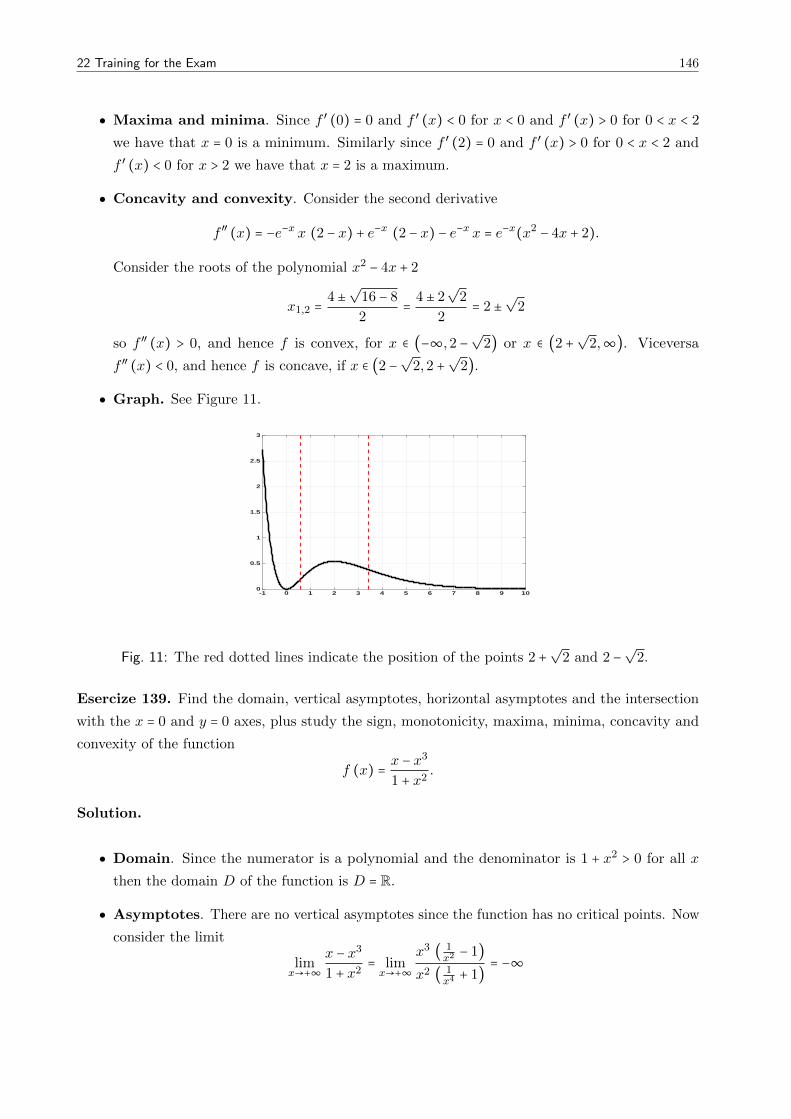
22 Training for the Exam 146
● Maxima and minima. Since f ′ (0) = 0 and f ′ (x) < 0 for x < 0 and f ′ (x) > 0 for 0 < x < 2
we have that x = 0 is a minimum. Similarly since f ′ (2) = 0 and f ′ (x) > 0 for 0 < x < 2 and
f ′ (x) < 0 for x > 2 we have that x = 2 is a maximum.
● Concavity and convexity. Consider the second derivative
f2 (x) = −e−x x (2 − x) + e−x (2 − x) − e−x x = e−x(x2 − 4x + 2).
Consider the roots of the polynomial x2 − 4x + 2
x1,2 =4 ±
√16 − 8
2= 4 ± 2
√2
2= 2 ±
√2
so f2 (x) > 0, and hence f is convex, for x ∈ (−∞,2 −√
2) or x ∈ (2 +√
2,∞). Viceversa
f2 (x) < 0, and hence f is concave, if x ∈ (2 −√
2,2 +√
2).
● Graph. See Figure 11.
-1 0 1 2 3 4 5 6 7 8 9 100
0.5
1
1.5
2
2.5
3
Fig. 11: The red dotted lines indicate the position of the points 2 +√
2 and 2 −√
2.
Esercize 139. Find the domain, vertical asymptotes, horizontal asymptotes and the intersection
with the x = 0 and y = 0 axes, plus study the sign, monotonicity, maxima, minima, concavity and
convexity of the function
f (x) = x − x3
1 + x2.
Solution.
● Domain. Since the numerator is a polynomial and the denominator is 1 + x2 > 0 for all x
then the domain D of the function is D = R.
● Asymptotes. There are no vertical asymptotes since the function has no critical points. Now
consider the limit
limx→+∞
x − x3
1 + x2= limx→+∞
x3 ( 1x2− 1)
x2 ( 1x4+ 1)
= −∞

22 Training for the Exam 147
limx→−∞
x − x3
1 + x2= limx→−∞
x3 ( 1x2− 1)
x2 ( 1x4+ 1)
= +∞
so there are no horizontal asymptotes.
● Intersection with x = 0. If x = 0 we get f (0) = 0.
● Intersection with y = 0. The equation
x − x3
1 + x2= 0
is equivalent to
x − x3 = x (1 − x2) = 0
and this is because 1 + x2 > 0 for all x. Hence the function intersects the axis y = 0 in x = 0
and x = ±1.
● Sign. Since, trivially, 1+ x2 ≥ 0 we have that f (x) ≥ 0 for all x such that x (1 − x2) ≥ 0 hence
for all x such that x ∈ (−∞,−1] or x ∈ [0,1].
● Monotonicity. Compute the first derivative
f ′ (x) = −x4 + 4x2 − 1
(x2 + 1)2
Hence
f ′ (x) ≥ 0⇔ x4 + 4x2 − 1 ≤ 0.
Put x2 = t and find the solution of
t2 + 4 t − 1 = 0
which are
t1,2 = −2 ±√
5.
Since t = x2 ≥ 0 only the solution −2 +√
5 is acceptable. So the equation
x4 + 4x2 − 1 = 0
has the two real solutions −√−2 +
√5 and +
√−2 +
√5. So the function is decreasing in
(−∞,−√−2 +
√5], increasing in [−
√−2 +
√5,+
√−2 +
√5] and decreasing in [+
√−2 +
√5,∞)
● Maxima and minima. Since f ′ (−√−2 +
√5) = 0 and f ′ (x) < 0 for x < −
√−2 +
√5 and
f ′ (x) > 0 for −√−2 +
√5 < x <
√−2 +
√5 we have that x = −
√−2 +
√5 is a minimum. Similarly
since f ′ (√−2 +
√5) = 0 and f ′ (x) > 0 for −
√−2 +
√5 < x <
√−2 +
√5 and f ′ (x) < 0 for
x >√−2 +
√5 we have that x =
√−2 +
√5 is a maximum.

22 Training for the Exam 148
● Concavity and convexity. Consider the second derivative
f2 (x) =4x (x2 − 3)(x2 + 1)3
so f2 (x) > 0, and hence f is convex, for x ∈ (−√
3,0) or x ∈ (√
3,∞). Viceversa f2 (x) < 0,
and hence f is concave, if x ∈ (0,√
3).
● Graph. See Figure 12.
-2 -1.5 -1 -0.5 0 0.5 1 1.5 2-1.5
-1
-0.5
0
0.5
1
1.5
Fig. 12: The red dotted lines indicate the position of the points −√−2 +
√5 and
√−2 +
√5. The
blue dotted lines indicate the position of −√
3 and√
3.
Esercize 140. Find the domain, vertical asymptotes, horizontal asymptotes and the intersection
with the x = 0 and y = 0 axes, plus study the sign, monotonicity, maxima, minima, concavity and
convexity of the function
f (x) = 2x + ln(1 − x1 + x
) .
Solution.
● Domain. The domain of
f (x) = 2x + ln(1 − x1 + x
)
coincides with the domain of ln (1−x1+x
). The logarithmic function ln (y) is defined if and only if
y > 0 so we need to impose that 1−x1+x > 0 which implies x ∈ (−1,1) so the domain is D = (−1,1).
● Asymptotes. There are two possible vertical asymptotes. Consider the limits in the critical
points x = −1 and x = 1. If x→ −1+ then 1−x1+x → +∞ and hence
limx→−1+
(2x + ln(1 − x1 + x
)) = +∞
so x = −1 is a vertical asymptote. If x→ 1− then 1−x1+x → 0+ and hence
limx→1−
(2x + ln(1 − x1 + x
)) = −∞

22 Training for the Exam 149
so x = 1 is a vertical asymptote. We cannot look for horizontal asymptotes given that the
domain of f is bounded.
● Intersection with x = 0. If x = 0 we get f (0) = 0.
● Intersection with y = 0. The equation
2x + ln(1 − x1 + x
) = 0 (22.2)
has at least the solution x = 0. From the sign of the derivative we can establish if this solution
is unique or note, so let’s move forward.
● Sign. We cannot say anything on the inequality
2x + ln(1 − x1 + x
) ≥ 0,
again we have to use the sign of the derivative to say more.
● Monotonicity. Compute the first derivative
f ′ (x) = − 2x2
1 − x2
so f ′ (x) < 0 for all x in the domain of the function, except for x ≠ 0. This means that the
function is strictly decreasing in its domain. Since f (0) = 0 this means that x = 0 is the
unique solution of the equation (21.3) and, besides, that f (x) > 0 for x < 0 and f (x) < 0 for
x > 0.
● Maxima and minima. Since f is strictly decreasing in its domain there are no maxima
and no minima.
● Concavity and convexity. Consider the second derivative
f2 (x) = − 4x
(x2 − 1)2
so f2 (x) > 0, and hence f is convex, for x < 0. Viceversa f2 (x) < 0, and hence f is concave, if
x > 0.
● Graph. See Figure 13.
Esercize 141. Find the domain, vertical asymptotes, horizontal asymptotes and the intersection
with the x = 0 and y = 0 axes, plus study the sign, monotonicity, maxima, minima, concavity and
convexity of the function
f (x) =√x
1 + ln (x)
Solution.

22 Training for the Exam 150
-1 -0.8 -0.6 -0.4 -0.2 0 0.2 0.4 0.6 0.8 1
-15
-10
-5
0
5
10
15
Fig. 13: The graph of f (x) = 2x + ln (1−x1+x
).
● Domain. The domain of
f (x) =√x
1 + ln (x)is determined by the conditions x > 0 (in order to have
√x and ln (x) defined) and ln (x) ≠ −1
(in order to have the denominator different from zero), which is equivalent to x ≠ e−1 = 1/e. So
the domain is D = (0,1/e) ∪ (1/e,∞).
● Asymptotes. There is one possible vertical asymptote at the critical point x = 1/e and one
at the critical point x = 0. If x→ (1/e)+ then 1 + ln (x)→ 0+ and hence
limx→(1/e)+
√x
1 + ln (x)= +∞
while if x→ (1/e)− then 1 + ln (x)→ 0− and hence
limx→(1/e)−
√x
1 + ln (x)= −∞.
Hence x = 1/e is a vertical asymptote. Nevertheless since
limx→0+
√x
1 + ln (x)= 0
−∞= 0.
then x = 0 it is not a vertical asymptote. Now consider
limx→∞
√x
1 + ln (x)= ∞∞
H= limx→∞
x
2√x= limx→∞
1
2
√x = +∞,
so there are no horizontal asymptotes.
● Intersection with x = 0. The point x = 0 is outside of the domain.
● Intersection with y = 0. The equation
√x
1 + ln (x)= 0 (22.3)

22 Training for the Exam 151
has no solution, since the numerator is zero at x = 0 but the denominator is not defined at
x = 0. Nevertheless we already know that the function√x
1+ln(x) approaches zero as x→ 0+.
● Sign. Since√x ≥ 0 always, the sign of
√x
1 + ln (x),
is equivalent to the sign of 1+ ln (x). Hence f (x) ≥ 0 if x ∈ (1/e,∞) and f (x) ≤ 0 if x ∈ (0,1/e).
● Monotonicity. Compute the first derivative
f ′ (x) = log(x) − 1
2√x(log(x) + 1)2
so f ′ (x) < 0 for all x < e (f is decreasing) and f ′ (x) > 0 for all x > e (f is increasing).
● Maxima and minima. By the considerations above x = e is a minimum and there are no
maxima.
● Concavity and convexity. Consider the second derivative
f2 (x) = 7 − log(x)(log(x) + 2)4x3/2(log(x) + 1)3
.
In order to find the zeros of f2 (x) we have to solve the equation
7 − log(x)(log(x) + 2) = 0,
which, putting y = log (x), is equivalent to
7 − y (y + 2) = 0
whose solutions are
y1,2 = −1 ± 2√
2
hence the solutions of 7 − log(x)(log(x) + 2) = 0 are
x1,2 = ey1,2 = e−1±2√2.
Hence the numerator of f2 (x) is positive for x ∈ (e−1−2√2, e−1+2
√2) while the denominator
is positive for (log(x) + 1)3 > 0 which is equivalent to log(x) + 1 > 0, that is for x > 1/e.So combining the sign of the numerator and of the denominator we get f2 (x) > 0 for
x ∈ (0, e−1−2√2), f2 (x) < 0 for x ∈ (e−1−2
√2,1/e), f2 (x) > 0 for x ∈ (1/e, e−1+2
√2) and
f2 (x) < 0 for x ∈ (e−1+2√2,∞).
● Graph. See Figure 13.

22 Training for the Exam 152
0 1 2 3 4 5 6 7 8 9 10-2
-1.5
-1
-0.5
0
0.5
1
1.5
2
Fig. 14: Blue lines represents the position of the points e−1±2√2. The magenta line is the vertical
asymptote x = 1/e while the red line is the position of the minimum x = e.