A stochastic model of soil erosion

INTERNATIONAL JOURNAL FOR NUMERICAL AND ANALYTICAL METHODS IN GEOMECHANICS. VOL. 8. 201-224 (1984)

A STOCHASTIC MODEL OF SOIL EROSION

MOSTAFA E. MOSSAADt AND TlEN H. WU Department of Civil Engineering, Ohio State University, Columbus, Ohio 43210 U.S.A.

SUMMARY

The erosion model computes the rill and inter-rill flow over a surface with random roughness, and the erosion caused by this flow. The measured roughness of a surface is analysed and used to generate random surfaces for the simulation process. Computations are carried out over a number of time intervals; the steady state condition is assumed for each interval. Changes in the surface geometry due to erosion during an interval are used to revise the surface for the subsequent interval. The model includes simplified mechanisms to simulate ponding, deposition and failure of side slopes of rills.

INTRODUCTION

The removal of soil on the earth's surface by moving water ranges from mass wasting on a geological scale to small scale erosion on construction sites. The process presents important problems to engineering, agriculture and geology. Because of the many factors that control erosion, the study of its mechanics involves several disciplines. One way to study a complex process like erosion is to construct a mathematical model that contains as many of the controlling factors as can be handled by the computing process and then perform numerical tests that will assess the influence exerted by these factors. Then, laboratory or field experiments can be designed to study the individual factors. This paper describes a first attempt at such a model and presents some of the results of simulations using this model.

The process of erosion begins when raindrops strike an inclined soil surface and detach soil particles from larger aggregates. In the case of some cohesive soils the detached particles may be composed of finer particles held together by physicakhemical forces. When the rainfall exceeds the infiltration rate, the overland flow begins and the detached soil particles are carried away. The overland flow tends to be concentrated in low areas, called rills, where erosion should also be most severe (e.g. Reference 1). Erosion during successive rainstorms deepens the rills and they become gullies. The quantity of soil eroded is clearly dependent on the microtopography of the eroded surface, which is composed of rills and inter-rill areas.' Hence a realistic erosion model should simulate the development of the eroded surface by computation of the erosion on different parts of the surface.

The random nature of the rill pattern and its contribution to the development of a drainage network was recognized by Horton? Leopold and Langbein' and Scheidegger; and simple simulations of topographical change, starting with an initial random surface have been presented by Schenck,' Seginer6 and Smart et al.' On a given surface, simplified as a plane, equations of sediment transport may be used to compute the amount of erosion, and various relations have been suggested by Foster and Me~er ,8 .~ Komura," Li et af." and Meyer and Wischmeier." Smith'' has developed a numerical model that accounts for variations in slope. Thus, it is

t Present address: Department of Civil Engineering, Cairo University, Cairo, Egypt.

0363-9061/84/030201-24$02.40 @ 1984 by John Wiley & Sons, Ltd.

Received 9 April 1982 Revised 18 October 1982

202 MOSTAFA E. MOSSAAD AND TIEN H. WU

timely to combine the equations of erosion with the; randomness of the surface topography in a model of the erosion on a sloped surface.

The overall objective of this research is to develop a mathematical model of the progress of erosion on sloping ground. It is required that the model should be able to account for the irregular topography of the ground surface, the pattern of overland flow that is compatible with the topography, and the erosion and topographic change that result from this flow.

To attain the objective, three principal tasks were completed: (1) analysis of ground surface roughness and construction of the random surface model, (2) study of sediment transport equations and construction of the erosion model and (3) construction of the simulation model that computes the erosion and topographical changes. In addition, tests were performed to evaluate the model’s sensitivity to several important parameters. Limited numerical experiments were made to compare model performance with empirical results.

The model presented here represents a first attempt and contains many simplifications out of necessity. Hence model predictions are only expected to provide order-of-magnitude estimates of the real process. Comparison of model performance with detailed experiments may be expected to identify shortcomings in the model and lead to refinements. In principle the model is not restricted to a particular scale. However, because of the importance of erosion on construction sites and reclaimed land, we have used data from erosion plots for this work.

SURFACE ROUGHNESS MODEL

The surface topography of a soil slope generally consists of a large number of humps of irregular shapes and sizes with depressions or rills between them. When overland flow moves downslope, the water tends to concentrate in the depressions, which constitute the flow paths.

A random surface model generates a surface which should have statistical properties as close as possible to those of the real surface. In addition, the numerical representation of the surface must be suitable for erosion computations. The trade-off between those two conditions is the main consideration in the formulation of the random surface model.

Method of spectral analysis

An elevation trace along any line on a slope surface, as shown in Figure 1 may be considered as a continuous function, y = f ( x ) . Then, Fourier analysis can be used to express this function as a sum of an infinite number of sinusoidal terms.

If each elevation trace represents a realization, then the group of traces in a measurement plot is considered to be an ensemble (see Figure 2). The classical method of analysing an ensemble in the time domain is to compute the autocorrelation function of each realization, then the overall autocorrelation function is calculated by averaging values of autocorrelation functions at each time lag.14 In spectral analysis, the spectrum of a process contains the same

DiSTANCE,x

Figure 1. Elevation trace

MODEL OF SOIL EROSION 203

A X . 2 cm R X)

- _/w* -* x

Figure 2. Measured t ram from experimental plot, Wooster (from Reference 18)

information given by the autocorrelation function, but in frequency domain. Accordingly, the overall spectrum of a process can be computed by averaging Fourier coefficients of the same harmonic component for all realizations. Then the average harmonic components are composed together to produce the spectrum.

According to Merva ef aL" a surface is called 'homogeneous' if the nature of the irregularity does not change from location to location. This condition is usually fulfilled in cases where mechanical treatment of the surface is the same at all locations. A surface is called isotropic if the statistical properties, along two orthogonal traces, are identical. When field measurements are made along parallel traces, as shown in Figure 2, they represent elevation variation only in one direction. When these data are used to generate a surface, the assumption of isotropy of the surface irregularities is implied. It is clear that such a condition does not Bold for ploughed surfaces, or for surfaces which have experienced considerable erosion.

We note that spectral analysis can be applied to the data in two dimensions to generate a random ~urface.'~~'' However, this prwedure would impose difficulties on the operation of the erosion model. Therefore, one-dimensional analysis is used in the present model.

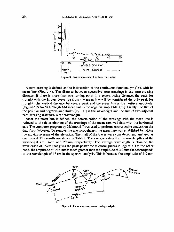
To study the nature of surface roughness, spectral analysis was applied to data from erosion plots at Wooster, Ohio." The plots were ploughed and then disked four times. Measurements of elevations were measured at points 2 cm apart along lines spaced at 7 cm (Figure 2). The results of spectral analysis are presented in the form of a power spectrum (Figure 3) which shows the power, or the contributions to the total variance, by different harmonic components.

The spectrum suggests that the roughness is composed of the macroroughness, or waves with lengths greater than 30 cm, and the microroughness, or waves with lengths less than or equal to 30 cm. The macroroughness represents topographical variations caused by tilling. Since the rills occupy the small depressions, their pattern will be controlled by the microroughness.

The method of zero-crossing analysis

Although spectral analysis can identify the relative importance of large scale and small scale roughness, it does not always help one to choose a representative wavelength or amplitude. The most direct method for analysis of roughness data is zero-crossing analysis.


5 2 0 1 L- , 2 1 0

i 10 20 30 40 50 WAVE N’ Ulvl DCK

198 3b 10 5 I WAVELENGTH (cm) 1 ;

+ro; micro-roughness 4 rough. pp Figure 3. Power spectrum of surface roughness

A zero crossing is defined as the intersection of the continuous function, y =f(x), with its mean line (Figure 4). The distance between successive zero crossings is the zero-crossing distance. If there is more than one turning point in a zero-crossing distance, the peak (or trough) with the largest departure from the mean line will be considered the only peak (or trough). The vertical distance between a peak and the mean line is the positive amplitude, (a+), and between a trough and mean line is the negative amplitude, ( L ) . Finally, the sum of the positive and negative amplitudes (a, + a-) is the waveheight and the sum of two adjacent zero-crossing distances is the wavelength.

After the mean line is defined, the determination of the crossings with the mean line is reduced to the determination of the crossings of the mean-removed data with the horizontal axis. The computer program by Mahmood’’ was used to perform zero-crossing analysis on the data from Wooster. To remove the macroroughness, the mean line was established by taking the moving average of the elevation. Then, all of the traces were considered and analysed as one record. The results are shown in Table I. The average values for the wavelength and the waveheight are 14cm and 29mm, respectively. The average wavelength is close to the wavelength of 18 cm that gives the peak power for microroughness in Figure 3. On the other hand, the amplitude of 14.5 mm is much greater than the amplitude of 3-7 mm that corresponds to the wavelength of 18 cm in the spectral analysis. This is because the amplitude of 3.7 mm

Meon

Figure 4. Parameters for zero-crossing analysis


Figure 5. Waves in zero-crossing analysis

represents only one component of the roughness spectrum. Thus, spectral analysis can identify the relative importance of large scale and small scale roughness. However, it does not provide data that allow one to choose a representative amplitude.

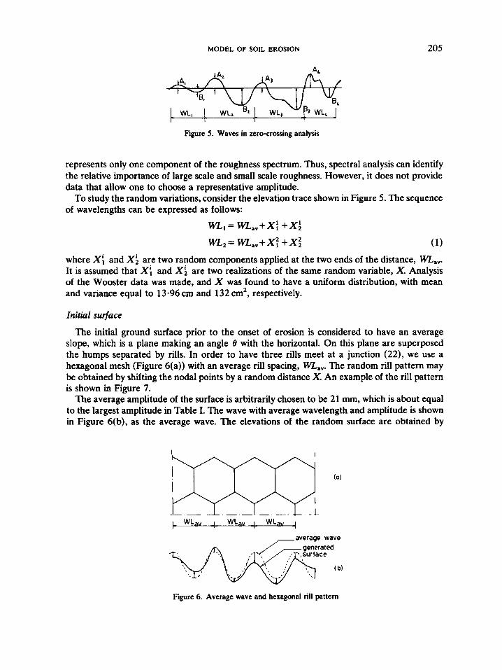
To study the random variations, consider the elevation trace shown in Figure 5. The sequence of wavelengths can be expressed as follows:

W L I = WL,,+x: +x: W L z = WL,,+x: +x: (1)

where Xf and Xi are two random components applied at the two ends of the distance, WL,,. It is assumed that Xf and Xi are two realizations of the same random variable, X. Analysis of the Wooster data was made, and X was found to have a uniform distribution, with mean and variance equal to 13.96 cm and 132 cm', respectively.

Initial surface

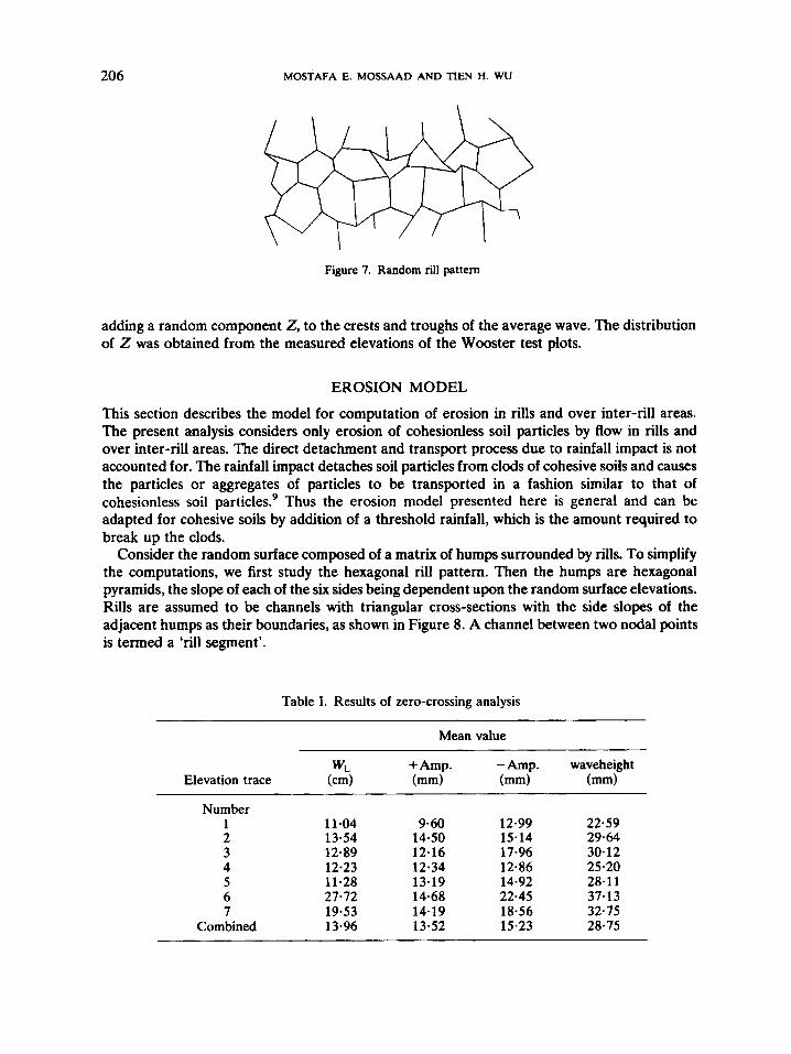
The initial ground surface prior to the onset of erosion is considered to have an average slope, which is a plane making an angle 8 with the horizontal. On this plane are superposed the humps separated by rills. In order to have three rills meet at a junction (22), we use a hexagonal mesh (Figure 6(a)) with an average rill spacing, WL,,. The random rill pattern may be obtained by shifting the nodal points by a random distance X. An example of the rill pattern is shown in Figure 7.

The average amplitude of the surface is arbitrarily chosen to be 21 mm, which is about equal to the largest amplitude in Table I. The wave with average wavelength and amplitude is shown in Figure 6(b), as the average wave. The elevations of the random surface are obtained by

I WL, , WL,, I WL," I -average wave

Figure 6. Average wave and hexagonal rill pattern

206 MOSTAFA E. MOSSAAD AND TIEN H. w u

Figure 7. Random rill pattern

adding a random component Z, to the crests and troughs of the average wave. The distribution of 2 was obtained from the measured elevations of the Wooster test plots.

EROSION MODEL

This section describes the model for computation of erosion in rills and over inter-rill areas. The present analysis considers only erosion of cohesionless soil particles by flow in rills and over inter-rill areas. The direct detachment and transport process due to rainfall impact is not accounted for. The rainfall impact detaches soil particles from clods of cohesive soils and causes the particles or aggregates of particles to be transported in a fashion similar to that of cohesionless soil particles.’ Thus the erosion model presented here is general and can be adapted for cohesive soils by addition of a threshold rainfall, which is the amount required to break up the clods.

Consider the random surface composed of a matrix of humps surrounded by rills. To simplify the computations, we first study the hexagonal rill pattern. Then the humps are hexagonal pyramids, the slope of each of the six sides being dependent upon the random surface elevations. Rills are assumed to be channels with triangular cross-sections with the side slopes of the adjacent humps as their boundaries, as shown in Figure 8. A channel between two nodal points is termed a ‘rill segment’.

Table I. Results of zero-crossing analysis

Mean value

W L Elevation trace (cm)

Number 1 11.04 2 13.54 3 12.89 4 12-23 5 11-28 6 27-72 7 19.53

Corn bined 13.96

+Amp. (mm)

-Amp. waveheight (mm) (mm)

9-60 14-50 12-16 12.34 13.19 14.68 14.19 13.52

12.99 15.14 17.96 12.86 14.92 22-45 18.56 15-23

22.59 29.64 30-12 25-20 28.11 37.13 32.75 28.75


a) PLan

b) Section A-A

Figure 8. Rill pattern and cross-section

Rill erosion

Consider a rill segment, ab, as shown in Figure 8(a). Let q1 =flow at a and q2=flow at b; q2 is greater than q1 by the amount of water drained from the two adjacent side slopes. The flow in the rill segment, ab, is a spatially-varied flow with lateral inflow from the side slope^.^^*'^*^^ However, since the present model deals with the erosion in short rill segments, equations of uniform flow are used.

Erosion due to rill flow is based on the concept of tractive force.21 Consider the triangular cross-section of a rill segment, as shown in Figure 9. The average value of the tractive force per unit wetted area, i.e. the unit tractive force, ro, is given by:

70 = 7RSf (2)

where y =unit weight of water, R =hydraulic radius of the channel, and &=slope of the energy grade line. For a mountain type channel, the slope of the energy line, S,, can be approximated by the bed slope, According to Chow,22 the unit tractive force in channels,

A = l h ' ( l + l ) = l h 2 c , 2 s, s, 2

sine, sine,

C , = I + - 1 sine, sine, P=h(-!-+-!--)= hc2

c,= c , /c, R = 1. hc,

2

Figure 9. Dimensions of rill cross-section

208 MOSTAFA E. MOSSAAD AND TlEN H. WU

except for wide open channels, is not uniformly distributed along the wetted perimeter. Therefore, it is more appropriate to use the tractive force per unit length of the rill as expressed by

Fo = TOP = ?AS0 (3) where P = wetted perimeter and A =cross-sectional area of the flow. In terms of the geometrical features of the cross-section (Figure 9), we have:

Neglecting the variation of So along the segment ab, the value of Fo is then dependent upon h. The values of hl at a and h2 at b depend on the flow rates, q1 and q2. To obtain the flow

depth, h, we use the well-known Manning equation,

( 5 ) V =- I R2/3S:/2

n

where V = the mean velocity in m/s, R = the hydraulic radius in m and n = the coefficient of roughness. Using the approximation S, = So and the relation q = VA we get:

This can be expressed in terms of h as:

q = (2 1 T) clh2 ($C~~)~ /~SA' '

2513- h = C l c j / 3 SO 112

(7)

where c1 and c3 are as defined in Figure 9. The flow in rills, treated as open channel flow, is used to compute the amount of soil eroded.

This assumes that the concentration of sediment is small enough so that the equation of motion for sediment-laden water can be approximated by the equation of motion for water only. According to Li et al." the continuity equation for sediment can be expressed as:

- Ps _- dqs dx (9)

where qs is the sediment discharge per unit width of channel and ps is the sediment pick-up rate per unit area. The bed load equation derived by Kalinske" is used to obtain qS. The reasons for the use of Kalinske's equation are primarily empirical. Komura" used it in a mathematical model for slope erosion by overland flow and established the range of values for some parameters in the equation. Calculations with these parameters led to results that are in reasonable agreement with measured rill erosion by Meyer et al.23 Kalinske's equation is

P

(10)


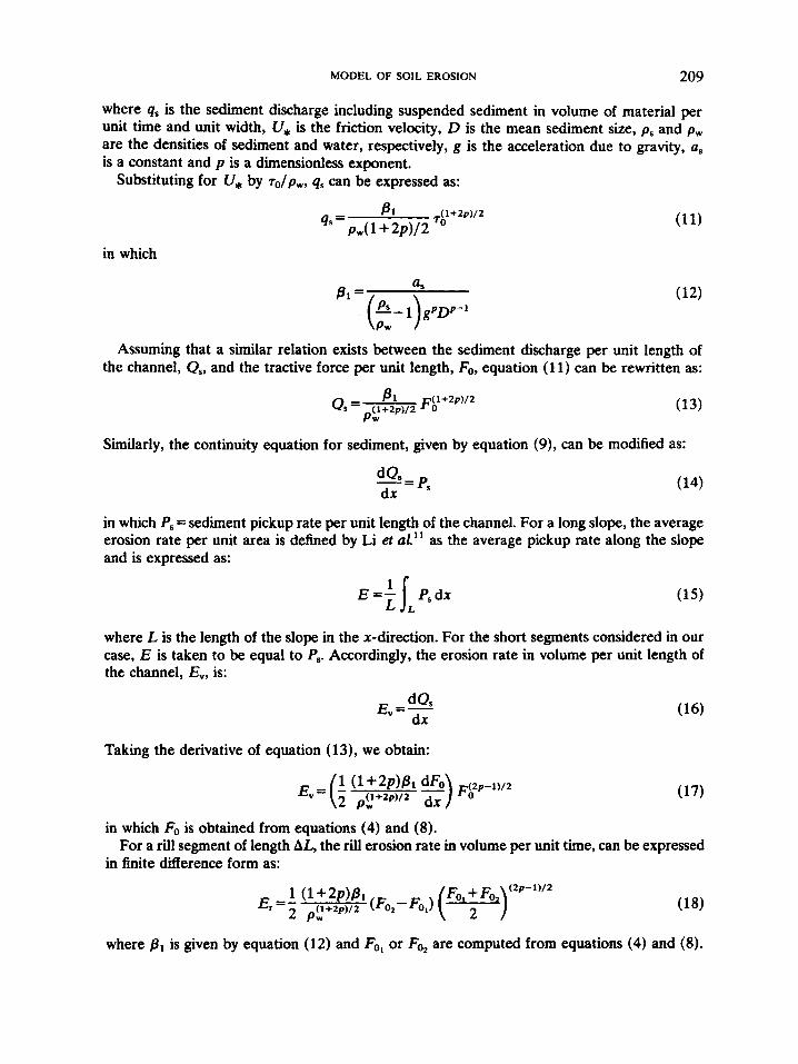
where qs is the sediment discharge including suspended sediment in volume of material per unit time and unit width, V, is the friction velocity, D is the mean sediment size, p , and pw are the densities of sediment and water, respectively, g is the acceleration due to gravity, a, is a constant and p is a dimensionless exponent.

Substituting for U, by r O / p w , qs can be expressed as:

in which

as (E- 1) gPDp-' B1=

Assuming that a similar relation exists between the sediment discharge per unit length of the channel, Q,, and the tractive force per unit length, Fo, equation (11) can be rewritten as:

Similarly, the continuity equation for sediment, given by equation (9), can be modified as:

in which P, = sediment pickup rate per unit length of the channel. For a long slope, the average erosion rate per unit area is defined by Li et aL" as the average pickup rate along the slope and is expressed as:

E = P, dx (15)

where L is the length of the slope in the x-direction. For the short segments considered in our case, E is taken to be equal to P,. Accordingly, the erosion rate in volume per unit length of the channel, Ev, is:

dQs E"=- dx

Taking the derivative of equation (13), we obtain:

in which Fo is obtained from equations (4) and (8).

in finite difference form as: For a rill segment of length AL, the rill erosion rate in volume per unit time, can be expressed

where B1 is given by equation (12) and Fo, or F,, are computed from equations (4) and (8).

210 MOSTAFA E. MOSSAAD AND TIEN H. W U

Inter-rill erosion

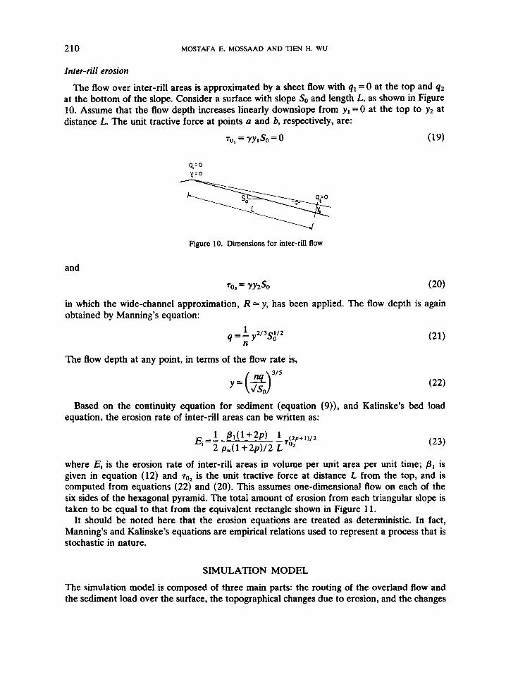
The flow over inter-rill areas is approximated by a sheet flow with q1 = O at the top and q2 at the bottom of the slope. Consider a surface with slope So and length L, as shown in Figure 10. Assume that the flow depth increases linearly downslope from y1 = O at the top to y, at distance L. The unit tractive force at points a and b, respectively, are:

To, = YY*So=O (19)

Figure 10. Dimensions for inter-rill flow

and

To2 = Y Y Z S O

in which the wide-channel approximation, R = y, has been applied. The flow depth is again obtained by Manning’s equation:

2/3 1/2 q=,y s o

The flow depth at any point, in terms of the flow rate is,

Y = ( 3)3/5 Based on the continuity equation for sediment (equation (9)), and Kalinske’s bed load

equation, the erosion rate of inter-rill areas can be written as:

where Ei is the erosion rate of inter-rill areas in volume per unit area per unit time; PI is given in equation (12) and T~~ is the unit tractive force at distance L from the top, and is computed from equations (22) and (20). This assumes one-dimensional flow on each of the six sides of the hexagonal pyramid. The total amount of erosion from each triangular slope is taken to be equal to that from the equivalent rectangle shown in Figure 11.

It should be noted here that the erosion equations are treated as deterministic. In fact, Manning’s and Kalinske’s equations are empirical relations used to represent a process that is stochastic in nature.

SIMULATION MODEL

The simulation model is composed of three main parts: the routing of the overland flow and the sediment load over the surface, the topographical changes due to erosion, and the changes

MODEL OF SOIL EROSION 21 1

equivalent rectan.

tual area

I Figure 11. Area for computation of inter-rill flow

in the erosion process with successive time intervals. In addition, there are several auxiliary mechanisms which affect erosion. These are ponding, failure of side slopes and low humps.

Routing of pow and sediment

The model assumes a constant run-off coefficient, RNF, which is the fraction of rainfall that becomes run-off. This part is divided between the rills and the inter-rills. The rain falling on the inter-rill areas drains to the surrounding rill segments as shown in Figure 12.

The rill flow and its sediment load at any nodal point of the hexagonal mesh depends on its location and elevation. The hexagonal mesh allows for two types of nodal points, as represented by points a and b in Figure 12. Point a receives flow from two branches and discharges it into one rill, whereas point b has only one inflow rill and the flow downslope is divided between two branches.

At points such as a in Figure 12, the flow from the two inflow branches is automatically directed to the outflow branch. But for points such as b, the inflow is divided between the outflow branches according to the ratio of the square root of the slopes, i.e. (So,/So2)1'2. This procedure is compatible with the exponent of slope in Mannings' formula, equation (5 ) . As for the sediment load, we use the ratio ( Sol/Soz)&'2p'1', which is obtained from equations (1 8) and (4).

Figure 12. Routing of rill and inter-rill Bows


The flow in rills moves forward only if the bed slope of the rill segment is positive. If the bed slope is either zero or negative, the flow routing of this rill is terminated at this point. The treatment of the flow at this point is described under ‘Ponding’.

Topographical change

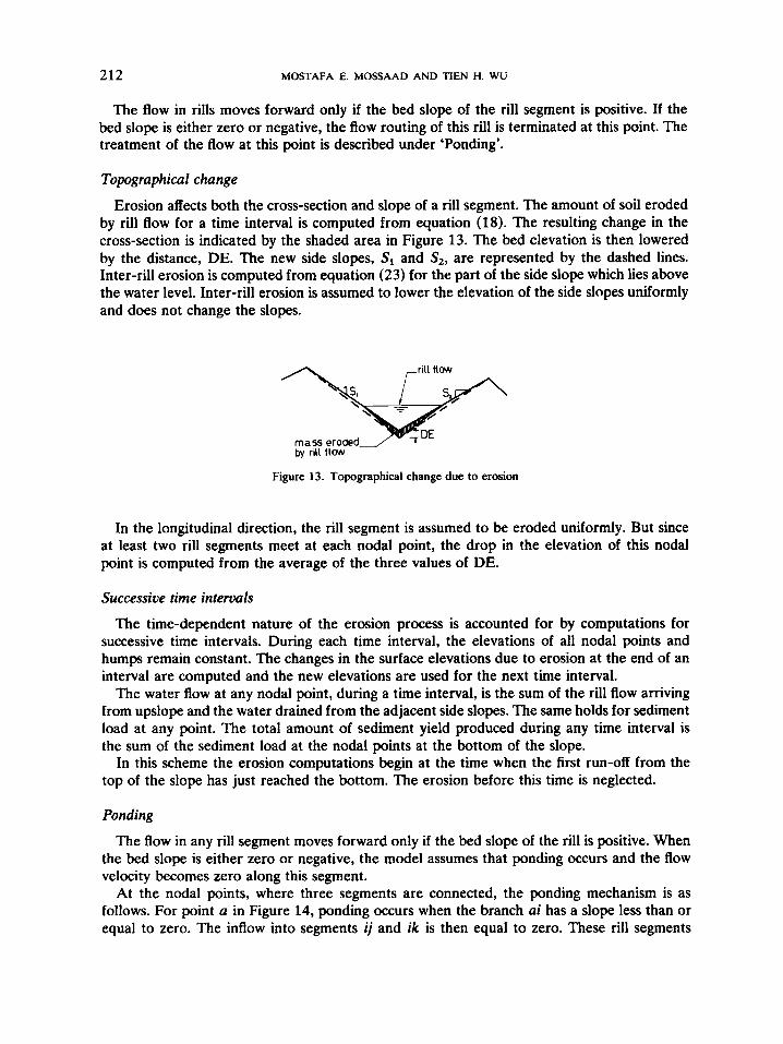
Erosion affects both the cross-section and slope of a rill segment. The amount of soil eroded by rill flow for a time interval is computed from equation (18). The resulting change in the cross-section is indicated by the shaded area in Figure 13. The bed elevation is then lowered by the distance, DE. The new side slopes, S, and S,, are represented by the dashed lines. Inter-rill erosion is computed from equation (23) for the part of the side slope which lies above the water level. Inter-rill erosion is assumed to lower the elevation of the side slopes uniformly and does not change the slopes.

Figure 13. Topographical change due to erosion

In the longitudinal direction, the rill segment is assumed to be eroded uniformly. But since at least two rill segments meet at each nodal point, the drop in the elevation of this nodal point is computed from the average of the three values of DE.

Successive time intervals

The time-dependent nature of the erosion process is accounted for by computations for successive time intervals. During each time interval, the elevations of all nodal points and humps remain constant. The changes in the surface elevations due to erosion at the end of an interval are computed and the new elevations are used for the next time interval.

The water flow at any nodal point, during a time interval, is the sum of the rill flow arriving from upslope and the water drained from the adjacent side slopes. The same holds for sediment load at any point. The total amount of sediment yield produced during any time interval is the sum of the sediment load at the nodal points at the bottom of the slope.

In this scheme the erosion computations begin at the time when the first run-off from the top of the slope has just reached the bottom. The erosion before this time is neglected.

Ponding

The flow in any rill segment moves forward only if the bed slope of the rill is positive. When the bed slope is either zero or negative, the model assumes that ponding occurs and the flow velocity becomes zero along this segment.

At the nodal points, where three segments are connected, the ponding mechanism is as follows. For point a in Figure 14, ponding occurs when the branch ai has a slope less than or equal to zero. The inflow into segments i j and ik is then equal to zero. These rill segments


Figure 14. Ponding conditions

then receive only water that is drained from adjacent side slopes. At point b in Figure 14, complete ponding occurs only if both bi and bj have slopes less than or equal to zero. When only one of the two branches is ponded, the flow is routed through the other branch.

Ponding influences the velocity of flow in rills located some distance upstream, and causes a reduction in the erosion rate in these rills. Consider the case when ponding occurs at point 1 in Figure 15(a) and the flow velocity in the segment 2-1 is zero at point 1. The sediment load arriving at point 1 is then deposited on the bottom of several rill segments upstream and downstream of point 1. It is arbitrarily assumed that the deposition of sediments raises the bottom of the rill segments by DE as shown in Figure 15(b). The change in the elevation of any point is the net difference between this deposition and the erosion computed from equations (18) and (23).

Failure of side slopes

The process of rill development is a combination of erosion, slumping of undercut side slopes, and head cuts. The progression of rill and inter-rill erosion steepens the side slopes and leads to slumping. The failure criterion used in this model consists of a limiting gradient, SLIMIT, that a side slope can withstand. When the gradient exceeds SLIMIT, the slope fails and assumes a flatter gradient, SSTART. The side slopes are assumed to remain plane, before and after failure.

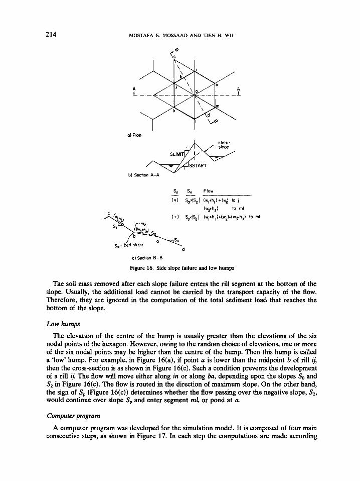
When a side slope fails, the top of the slope, which is the centre of the hump, is lowered as shown in Figure 16. Some of the sides of the hump may fail whereas others may be stable. Therefore, the computations give different elevations at the tops of different slopes. At the end of an interval, the elevation of the hump centre is taken to be the average of the top elevations of the six side slopes.

I I'o I' f2 I w pond ed point

a) Segments affected by ponding b)Deposition pattern

Figure 15. Deposition due to ponding


a) Plan

S, So Flow

( + I S,,(Sz( (wl+hl )+($ to j - -

(wgh3) to ml

so= bed slope d

(wl+hl to rnl

C ) SectlOn 8- B

Figure 16. Side slope failure and low humps

The soil mass removed after each slope failure enters the rill segment at the bottom of the slope. Usually, the additional load cannot be carried by the transport capacity of the flow. Therefore, they are ignored in the computation of the total sediment load that reaches the bottom of the slope.

Low humps

The elevation of the centre of the hump is usually greater than the elevations of the six nodal points of the hexagon. However, owing to the random choice of elevations, one or more of the six nodal points may be higher than the centre of the hump. Then this hump is called a ‘low’ hump. For example, in Figure 16(a), if point a is lower than the midpoint b of rill ij, then the cross-section is as shown in Figure 16(c). Such a condition prevents the development of a rill ij. The flow will move either along in or along ba, depending upon the slopes So and S, in Figure 16(c). The flow is routed in the direction of maximum slope. On the other hand, the sign of S, (Figure 16(c)) determines whether the flow passing over the negative slope, S,, would continue over slope S, and enter segment ml, or pond at a.

Computer program

A computer program was developed for the simulation model. It is composed of four main consecutive steps, as shown in Figure 17. In each step the computations are made according

MODEL OF SOIL EROSION

I

215

ANALYSIS OF SURFACE ROUGHNESS DATA

Subroutines associated wi th d i f f e r e n t steps:

YES

Store values o f t o t a l erosion for t h i s randm surface

I n i t i a l i z e arrays o f flow, erosion, and elevation L New surface

I

START

GENERATION OF A RANDOM SURFACE

I A + l COMPUTATION

I 'W

WAVE TERPI FILTER RESDL POWER

HXCISH RANOM ELEVTN SFAI LR HUMP ACJNT RAM)U

POND FLOW RDlSTB

ERSNl HERSN ERSNl RERSN I DHnP SNEGTV CSEC

1

I I I n i t i a l i z e arrays o f erosion and f low quant i t ies Replace o ld elevations I ' I I w NT = N T I

M NS = NRS

6 Figure 17. Computational scheme

to the rules established in the preceding sections. These steps are repeated for successive time intervals until the end of the test period.

SENSITIVITY ANALYSIS

This section considers the sensitivity of the model to the different parameters and factors. Since the computer program is long, a preliminary study was made to determine reasonable time and space intervals that should be adopted. Accordingly, the effect of the time interval and the dimensions of the test area were tested first. Next, we examined the sensitivity of the model to the parameters n, a, and p, which appear in equations (8) and (12). Finally, the sensitivity of the model to randomness in the rill pattern was investigated.


Geometrical limitations

The width of the hexagonal element is taken to be the length of the average wave. Tests were conducted using a rectangular area covered by a 20 X 50 mesh and a 50 X 20 mesh. The results for the 20 x 50 mesh show large fluctuations in the erosion rate vs. time.

A closer study of the numerical scheme indicated that this phenomenon is related to ponding. If the width of the test area is small, then ponding at any rill segment, especially those near the bottom of the slope, causes a significant drop in erosion rate. Then, in subsequent intervals, when deposition elevates a point and removes the ponding situation, the erosion rate increases.

The erosion rate vs time curve for a 50 X 20 mesh, subjected to the same rainfall, has much smaller fluctuations. To keep the fluctuations small, subsequent runs were conducted using a 65 X 30 mesh.

lime interval

The effect of the length of time interval is important in dynamic simulation models. Results of calculations with time intervals ranging from 2.0 to 360 min indicate a significant change in the shape of the erosion vs. time curve with increasing time interval. The erosion rate at any time is larger for shorter intervals. This is attributed to the change in side slopes after slope failure and the effect of updating the elevations after each time interval. To avoid excessive computation costs, a time interval of 10 min was adopted for the rest of the study. The computed erosion rate is about 0.80 of that obtained with the smallest time interval of 2 min.

Parameters in erosion equations

The erosion model uses the Manning equation ( 5 ) to compute the flow in rills and over inter-rill areas. Therefore, it is important to investigate the effect of Manning's coefficient, IL Other important parameters in the erosion model are p and a, in Kalinske's bed load equation (10). However, a, for rill erosion may be considerably different from a, for inter-rill erosion. Therefore, a, in the rill erosion equation (18) is denoted by ASR, and a, in the inter-rill erosion equation (23) is denoted by ASH. The values adopted for different parameters in the sensitivity analysis are listed in Table 11.

Table 11. Parameters used in sensitivity analysis

Parameters fixed during the analysis

Mesh = 65 X 30 Rainfall = 64 mm/h Time interval = 10 min D=O*O1 mm Slope = 20" = 37 per cent SSTART = 1 * 1

Parameters varied during the analysis*

n = 0-02,0.03, (0.04), 0.05 ASR = 200,300, (400), 500 ASH = 10, (20), 30,40 p=(1-5), 1.75,2,2*5 SLIMIT=1-1,1*2,1*3, (1.4)

* Values in parentheses were used when testing other parameters

The value of n is strongly dependent on the roughness of the surface over which water flows. Values of n have been reported by Chowz2 for a variety of cases. However, because of the small scale at which the erosion is modelled, it is difficult to choose the appropriate value. To test the model, values of 0-02, 0-03,0.04 and 0.05 were used for n.


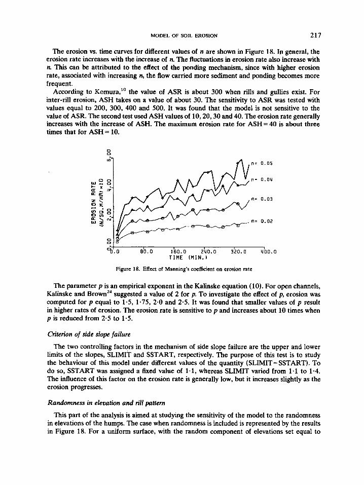
The erosion vs. time curves for different values of n are shown in Figure 18. In general, the erosion rate increases with the increase of n. The fluctuations in erosion rate also increase with n. This can be attributed to the effect of the ponding mechanism, since with higher erosion rate, associated with increasing n, the flow carried more sediment and ponding becomes more frequent.

According to Komura," the value of ASR is about 300 when rills and gullies exist. For inter-rill erosion, ASH takes on a value of about 30. The sensitivity to ASR was tested with values equal to 200, 300, 400 and 500. It was found that the model is not sensitive to the value of ASR. The second test used ASH values of 10,20,30 and 40. The erosion rate generally increases with the increase of ASH. The maximum erosion rate for ASH = 40 is about three times that for ASH= 10.

0 0

n= 0.05

n - 0.011

fl= 0.03

n= 0.02

I cb'. 0 80.0 160.0 240.0 3 > 0 3 0 0 . 0 T I H E ( t l I N . 1

Figure 18. Effect of Manning's coefficient on erosion rate

The parameter p is an empirical exponent in the Kalinske equation (10). For open channels, Kalinske and Brownz4 suggested a value of 2 for p. To investigate the effect of p, erosion was computed for p equal to 1.5, 1.75, 2.0 and 2-5. It was found that smaller values of p result in higher rates of erosion. The erosion rate is sensitive to p and increases about 10 times when p is reduced from 2.5 to 1.5.

Criterion of side slope failure

The two controlling factors in the mechanism of side slope failure are the upper and lower limits of the slopes, SLIMIT and SSTART, respectively. The purpose of this test is to study the behaviour of this model under different values of the quantity (SLIMIT-SSTART). To do so, SSTART was assigned a fixed value of 1.1, whereas SLIMIT varied from 1.1 to 1-4. The influence of this factor on the erosion rate is generally low, but it increases slightly as the erosion progresses.

Randomness in elevation and rill pattern

This part of the analysis is aimed at studying the sensitivity of the model to the randomness in elevations of the humps. The case when randomness is included is represented by the results in Figure 18. For a uniform surface, with the random component of elevations set equal to


Figure 19. Location of samples of flow, uniform rill pattern

zero, the erosion rate increases nearly uniformly with time, with little or no fluctuation. The uniform surface also has rates of erosion that are about 2.5 times those of the random surface. This is because the uniform surface has fewer obstacles and less possibility of ponding.

To evaluate the effect of the simplification introduced by the hexagonal rill pattern, the model predictions are compared with that of a model using a random rill pattern. Since the amount of'soil eroded at any point is directly related to the flow at that point, we chose to use the flow as a basis for comparison. A 15x8 mesh surface with an average slope of 20" was used in the comparison. A unit of water enters each rill at the top of the slope and the flow was computed for rill segments located on the 4th row and 6th row from the top of the slope as shown in Figures 19 and 20. Each row contains 14 segments. The mean flow for hexagonal rill pattern is about 1.5 times that for the random rill pattern. The flow for the hexagonal rill pattern has a larger variance than that for the random rill pattern.

Summary on sensitivity

The sensitivity tests have shown that the parameters p, n and ASH have the greatest influence on the computed erosion. For the ranges in p, n and ASH tested, the highest computed erosion rates are respectively 10, 5 and 3 times the lowest erosion rates. The random components of surface roughness and rill pattern, ponding and low humps all tend to reduce the computed erosion. The adoption of the hexagonal mesh for the initial rill pattern does not significantly affect the computed erosion. We note that because of low humps and rill capture, an irregular rill pattern soon develops over the hexagonal mesh.

MODEL PERFORMANCE

The erosion model was tested by comparison of the model performance with results of field experiments. However, the data obtained in most field studies do not contain all the model

\ I / r I

samp(e for -test no 1

sample for lest no 2

Figure 20. Location of samples of flow, random rill pattern


parameters. Hence, only order-of-magnitude comparison for one case was made. An evaluation of the general performance of the model can be made by studying the influence of slope gradient and rainfall intensity on predicted erosion. Since there is plenty of empirical evidence on the influence of these conditions on erosion, general comparisons can be made to see if the model performance is qualitatively in agreement with empirical knowledge.

Comparison with field measurements

Results of erosion measurements from highway embankments were compared with model predictions. In the study by Barnett et aLZS seven plots at each of four locations were prepared with different treatments. One of these was left with a bare surface. Each site was graded to 24: 1 slope, seeded, rototilled and then firmed with a cultipacker. At two of the four locations, the soil was classified as clay. The soil at the other two locations was classified as sandy clay loam. The test storm was applied at an intensity of 6.25cm per hour in two increments of 20 min each. The first increment, 3.13 cm in 30 min, corresponds to a one-year frequency storm; the entire test represents a 10-year frequency storm for that region of Georgia.

Among the many parameters that are needed as input to the model, ASR, ASH and p are common for slope erosion problems. On the other hand, the representative size of soil particles, the Manning's coefficient, and the surface roughness must be determined for each site. Since such data are not available for the test plots, it was necessary to assume reasonable values for the calculations. The surface roughness data obtained from Wooster, Ohio, were assumed to represent a well-cultivated surface, and used in the computations. To estimate Manning's coefficient, use was made of the results of the investigation by Ree et ~ 1 . ~ ~ Values as high as 0.3 were reported in their study for poor-cover conditions. Far the bare surface in question, computations were made for a range of n from 0.025 to 0.2. According to Foster and M e ~ e r , ~ clay particles are detached by rainfall as aggregates and move along the bottom of the rills as cohesionless particles. This observation was used as the basis for the choice of the representative diameter, D. For the plot classified as clay, the reported gradation is 39 per cent sand, 27 per cent silt and 34 per cent clay. To represent the clay aggregates and the non-aggregated sand and silt, the value of 0.01 mm was selected for D. For the second plot, with the gradation of 57 per cent sand, 17 per cent silt and 26 per cent clay, D was taken to be 0.05 mm.

Using a time interval of 2 min, the total soil loss at the middle, and at the end of a 60-min storm period were computed. The results indicate that in order to achieve soil losses comparable to the measured values, the Manning's coefficient n should be around 0.085 for the clay site and over 0.2 for the sandy clay site. For a bare slope, these values are higher than the estimates by Ree et dZ6 In view of possible errors in the other parameters, particularly Kalinske's coefficient p, this discrepancy is not considered to be too serious.

Influence of physical conditions

The slope of a surface is one of the most important factors in erosion. However, a unique relation between slope and erosion has not been established." The model was used to compute the erosion for four plots with slopes of 5, 10, 15 and 20". The results indicate that steeper slopes result in larger erosion rates. However, the relation between slope gradient and erosion rate is time-dependent. This may be one reason for the differences between the results of various experimental studies on the effect of slope gradient on the erosion rate.

Three storms with rainfall intensities of 50, 25 and 12-5 mm/h, with rain periods of 3, 6 and 12 hours, respectively, were used for erosion computations. At the end of each period, the plots would receive the same rainfall of 150 mm. The storms were applied to plots with


10 20 30 40 50 RAINFALL INTENSITY

(rnm/hr)

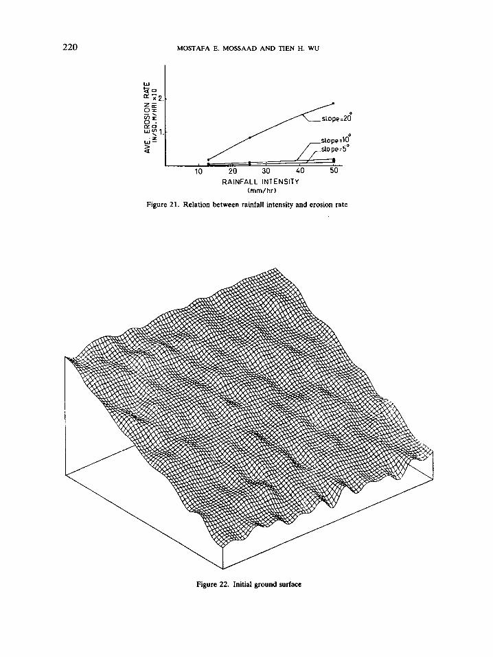
Figure 21. Relation between rainfall intensity and erosion rate

Figure 22. Initial ground surface

MODEL OF SOIL EROSION 22 1

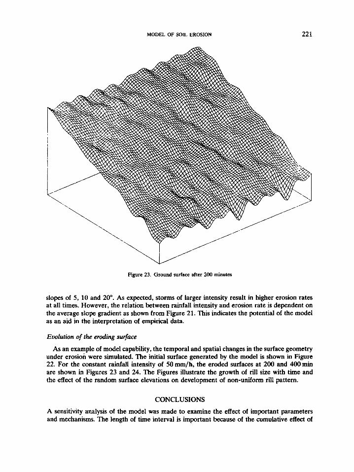
Figure 23. Ground surface after 200 minutes

slopes of 5 , 10 and 20". As expected, storms of larger intensity result in higher erosion rates at all times. However, the relation between rainfall intensity and erosion rate is dependent on the average slope gradient as shown from Figure 21. This indicates the potential of the model as an aid in the interpretation of empirical data.

Evolution of the eroding surface

As an example of model capability, the temporal and spatial changes in the surface geometry under erosion were simulated. The initial surface generated by the model is shown in Figure 22. For the constant rainfall intensity of 50 mm/h, the eroded surfaces at 200 and 400 min are shown in Figures 23 and 24. The Figures illustrate the growth of rill size with time and the effect of the random surface elevations on development of non-uniform rill pattern.

CONCLUSIONS

A sensitivity analysis of the model was made to examine the effect of important parameters and mechanisms. The length of time interval is important because of the cumulative effect of


Figure 24. Ground surface after 400 minutes

the surface-updating procedure. Therefore, shorter time intervals give better estimates of erosion rate. Manning’s coefficient and Kalinske’s coefficients have the strongest influence on the erosion rate.

The model predictions were compared with data from field experiments. The limited tests that have been carried out indicate that the model calculates erosion rates that are of the right order of magnitude. The model performance is also in general agreement with empirical knowledge on the influence of slope length and rainfall intensity. It is realized that the tests are very approximate in nature and do not provide a verification of the model. An adequate test of the model would require a specially designed field experiment in which all important model inputs and outputs are measured.

The present model must be considered as preliminary. Stochastic modelling is limited to the ground surface characteristics and flow routing. Improvements in understanding of overland flow and sediment transport should enable the extension of stochastic modelling to these two important elements.


ACKNOWLEDGEMENTS

This research was supported by a grant from the Office of Water Research and Technology, U.S. Department of Interior, under project A056-Ohio. The writers are grateful to K. W. Bedford and V. T. Ricca for their advice, which is crucial in the development of the erosion model; to E. M. Ali and K. Mahmood for their assistance with spectral analysis and zero-crossing analysis, respectively; and to D. M. Van Doren Jr., who kindly provided us with the surface roughness data from Wooster.

NOTATION

a, =constant in Kalinske’s equation A = area of channel Ei = inter-rill erosion rate E, = rill erosion rate Fo = tractive force per unit length of channel g = gravitational acceleration h =depth of channel n = Mannings coefficient p =constant in Kalinske’s equation P = wetted perimeter p, = sediment pickup rate per unit area of channel P, = pickup rate per unit length of channel q =rate of flow

Q, = sediment discharge per unit length of channel R = hydraulic radius So = bed slope V = velocity y = unit weight of water p, = mass density of sediment

pw = mass density of water T~ = unit tractive force per unit area of channel

REFERENCES

1. L. D. Meyer, D. C. DeCouney and M. J. M. Romkens, ‘Soil erosion concepts and misconceptions’, Proceedings of the third Federal Inter-Agency Sedimentation Conference, Water Resource Council, March 22-23, Denver, CO, (1976).

2. R. E. Horton, ‘Erosional development of streams and their drainage basins; hydrophysical approach to quantitative morphology’, Geol. Soc. America Bull. 56, 275-370 (1945).

3. L. B. Leopold and W. B. Langbein, ‘The concept of entropy in landscape evolution’, U.S. Geol. Sum. Profess. Paper 500-A (1962).

4. A. E. Scheidegger, ‘A stochastic model for drainage patterns into an intramontane trench’, Bull. Inr. ASS. ofsci. Hydrol. 12, 15-20 (1967).

5. H. Schenk, ‘Simulation of the evolution of drainage basin networks with a digital computer’, J. Geophys. Res. 68,

6. I. Seginer, ‘Random walk and random roughness models of drainage networks’, Wafer Resources Research, 5,

7. J. S. Smart, A. J. Surkan and J. P. Considine, ‘Digital simulation of channel networks’, in Symposium on River Morphology, General Assembly of Bern, 87-98, 1967.

8. G. R. Foster and L. D. Meyer, ‘A closed-form soil erosion equation for upland areas’, in H. W. Shen (ed.), Sedimentation: Symposium To Honor Professor H. A. Einstein, 12.1-12.19. H. W. Shen, Fort Collins, 1972.

(20). 5739-5745 (1963).

(3), 591-607 (1969).

224 MOSTAFA E. MOSSAAD AND T E N H. WU

9. G. R. Foster and L. D. Meyer, ‘Transport of soil particles by shallow flow’, Transactions of the Amer. Soc. of

10. S . Komura, ‘Hydraulics of slope erosion by overland flow, Joumul of the Hydraulics Division, Amer. Soc of Ciu.

11. R. M. Li, H. W. Shen and D. B. Simons, ‘Mechanics of soil erosion by overland flow, Proceedings ofthe 15rh

12. L. D. Meyer and W. H. Wischmeier, ‘Mathematical simulation of the process of soil erosion by water’, Transadions

13. R. E . Smith, ‘Simulating erosion dynamics with a deterministic distributed watershed model’, Proc. 3rd Federal

14. D. E. Newland, An Introduction to Random Vibrations and Spectral AMIYS~S, Longman, London, 1975. 15. G. E. Merva, R. D. Brazee, G. 0. Schwab and R. B. Curry, ‘Theoretical considerations of watershed surface

16. J. Rayner, A n Introduction to Spectral Analysis, Academic Press, New York, NY, 1971. 17. M. Shinozuka and C. M. Jan, ‘Digital simulation of random processes and its applications’, Journal of Sound and

18. D. M. Van Doren Jr., Personal communication, 1978. 19. K. Mahmood and H. Ahmadi-Karvigh, Statistical Procedures for Bed Form Anulysis, CERTS-76-KM-HAK 41,

20. Y. N. Yoon and H. G. Wenzel, ‘Mechanics of sheet flow under simulated rainfall’, Journal of the Hydraulics

21. W. H. Graf, Hydraulics of Sediment Transport, McGraw-Hill, New York, 1971. 22. V. T. Chow, Open-Channel Hydraulics, McGraw-Hill, New York, 1959. 23. L. D. Meyer, G. R. Foster and S. Nikolov, ‘Effect of flow rate and canopy on rill erosion’, Transactions of the

24. H. Rouse, Engineering Hydraulics, Wiley New York, 1949. 25. A. P. Barnett, E. G. Diseker and E. C. Richardson, ‘Evaluation of mulching methods for erosion control on newly

26. W. 0. Ree, F. L. Wimberley and F. R. Crow, ‘Manning and the overland flow equation’, Transactions of the

27. F. M. Henderson, Open Channel Flow, MacMillan. New York, 1966.

Agr. Eng. 15, ( l ) , 99-102 (1972).

Eng. 102, (HYlO), 15731586 (1976).

Congress, Inremutionul Associutwn for Hydraulics Research, Istanbul, Turkey, 1, 437-446 (1973).

of the Amer. Soc. of Agr. Eng. 12, (6). 754-758. 762 (1969).

Interagency Sediment Conference, 1976.

description’, Transactions of Amer. Soc. of Agr. Eng. 13, (4). 462-465 (1970).

Vibrations, 25, (1). 111-128 (1972).

Engineering Research Centre, Colorado State University, Fort Collins, CO, 1976.

Dioision, Amer. Soc. of Civil Eng. 97, (HY9), 1367-1368 (1971).

Amer. Soc of Agr. Eng. 18(5), 905-911 (1975).

prepared and seeded highway backslopes’, Agronomy Journal, 59, 83-85 (1967).

Amer. SOC. of Agr. Eng. 19, (8). 89-95 (1976).

A stochastic model of soil erosion

Documents

Transcript of A stochastic model of soil erosion