ORI GIN AL PA PER

Soil erosion susceptibility assessment and validationusing a geostatistical multivariate approach: a testin Southern Sicily

Christian Conoscenti Æ Cipriano Di Maggio Æ Edoardo Rotigliano

Received: 15 May 2007 / Accepted: 18 October 2007 / Published online: 26 February 2008� Springer Science+Business Media B.V. 2008

Abstract A certain number of studies have been carried out in recent years that aim at

developing and applying a model capable of assessing water erosion of soil. Some of these

have tried to quantitatively evaluate the volumes of soil loss, while others have focused

their efforts on the recognition of the areas most prone to water erosion processes. This

article presents the results of a research whose objective was that of evaluating water

erosion susceptibility in a Sicilian watershed: the Naro river basin. A geomorphological

study was carried out to recognize the water erosion landforms and define a set of

parameters expressing both the intensity of hydraulic forces and the resistance of rocks/

soils. The landforms were mapped and classified according to the dominant process in

landsurfaces affected by diffuse or linear water erosion. A GIS layer was obtained by

combining six determining factors (bedrock lithology, land use, soil texture, plan curva-

ture, stream power index and slope-length factor) in unique conditions units. A

geostatistical multivariate approach was applied by analysing the relationships between the

spatial distributions of the erosion landforms and the unique condition units. Particularly,

the density of eroded area for each combination of determining factors has been calculated:

such function corresponds, in fact, to the conditional probability of erosion landforms to

develop, under the same geoenvironmental conditions. In light of the obtained results, a

general geomorphologic model for water erosion in the Naro river basin can be depicted:

cultivated areas in clayey slopes, having fine-medium soil texture, are the most prone to be

eroded; linear or diffuse water erosion processes dominate where the topography is

favourable to a convergent or divergent runoff, respectively. For each of the two erosion

process types, a susceptibility map was produced and submitted to a validation procedure

based on a spatial random partition strategy. Both the success of the validation procedure

of the susceptibility models and the geomorphological coherence of the relationships

between factors and process that such models suggest, confirm the reliability of the method

and the goodness of the predictions.

C. Conoscenti � C. Di Maggio � E. Rotigliano (&)Dipartimento di Geologia e Geodesia, Universita degli Studi di Palermo,Via Archirafi 20, Palermo 90123, Italye-mail: rotigliano@unipa.it

123

Nat Hazards (2008) 46:287–305DOI 10.1007/s11069-007-9188-0

Keywords Water erosion � GIS � Multivariate statistical analysis � Validation �Naro river basin � Southern Italy � Sicily

1 Introduction

Water erosion is a problem of great importance because of its social and economic impact.

It is, in fact, responsible both for direct damages, as it erases the productive interface of

outcropping rocks (soil), and for indirect damages, as in its most intense linear evidences, it

can lead to or reactivate surficial landslides, by locally increasing the steepness of the

slopes.

Several methods have been implemented and applied to assess soil loss, mainly clas-

sified into two types: empirical and physically-based. The empirical methods estimate soil

erosion by combining a prefixed set of physical parameters, based on certain standardized

coefficients or procedures, which have been optimized from empirical observations in

sample areas (test basins or plots). These methods have been applied quite extensively,

despite the fact that they have been implemented in regions characterized by specific

physical conditions. The most commonly adopted empirical methods are the Universal Soil

Loss Equation (USLE; Wischmeier and Smith 1965) and its reviewed models (e.g.,

MUSLE and RUSLE). An empirical method that exploits the relationships between the

mean annual observed suspended load and the quantitative geomorphic attributes of the

drainage networks, has been developed for the Italian basins (Ciccacci et al. 1981). The

physically-based methods mathematically (e.g., the WEPP model; Nearing et al. 1989)

describe the process of detachment, transportation and deposition of the eroded soil. These

methods can easily be exported to different environments, but they require a large and

extremely detailed set of parameters, which are often not available on a basin scale.

The methods described above analyse soil erosion by trying to estimate the volumes or

masses of soil loss. However, it is possible to approach the study of soil erosion by

observing the geostatistical spatial relationships between the physical determining factors

and the effects of the process: the erosion landforms. This approach is based on repro-

ducible steps, quantitative and well linked to the climatic and geological features of the

studied area, as it does not refer to equations and coefficients set up and calibrated for

specific areas elsewhere in the world; rather it is directly based on the evidences (the water

erosion landforms) of processes that have been driven by specific climatic and geologic

conditions. The main goal of this kind of method is to differentiate the investigated areas

on the basis of their susceptibility degrees, in terms of the propensity of erosion landforms

occurring in the future, rather than to quantify tons or cubic metres of soil loss. Erosion

landforms are, in fact, evidence of the action of soil erosion, and are easily and quickly

recognizable by remote and field surveys.

Among the geostatistical methods, the one proposed by Marker et al. (1999) is based on

the concept of the Erosion Response Units (ERU): ‘‘distributed three-dimensional terrain

units, which are heterogeneously structured; they each have homogeneous erosion process

dynamics characterized by a slight variance within the unit, if compared to neighbouring

ones, and they are controlled by their physiographic properties, and the management of

their natural and human environment’’. The ERU model allows the scientist to obtain

information about the entire river basin’s susceptibility to erosion, by characterizing the

distribution of erosion processes in limited portions.

288 Nat Hazards (2008) 46:287–305

123

Water erosion processes in some basins in Western Sicily have been studied since the

beginning of 2002, in the framework of two National Research projects focused on the

analysis of soil erosion in Mediterranean areas (Agnesi et al. 2006; Conoscenti et al.

2006).

In the present research, a multivariate analysis has been applied to evaluate water

erosion susceptibility in a river basin whose geological, topographic and climatic features

are similar to those of other wide sectors of Sicily (Agnesi et al. 2006; Conoscenti et al.

2007). The method here proposed is based on a multivariate geostatistical approach that

exploits a probabilistic function, contrary to that of the ERU model, which corresponds to

the spatial density of erosion landforms in homogeneous domains; these are defined in

terms of their specific combination of physical controlling factors and correspond to the

concept of the Unique Conditions Unit (UCU), widely adopted in landslide hazard studies

(Carrara and Guzzetti 1995). Furthermore, a validation procedure based on a spatial ran-

dom partition strategy has been applied to test the effectiveness of the predictive models.

2 Study area

The Naro river basin, situated in the middle of Southern Sicily, has an area of about

250 km2 and flows from NE to SW into the Sicilian Channel (Fig. 1a). According to

Catalano et al. (1993), it is located in the mildly folded foredeep—foreland sector of the

Sicilian collisional complex, and is characterized by the outcroppings of the following:

conglomerates, clayey sandstones and marls (Terravecchia Fm., Upper Tortonian-Lower

Messinian); diatomites, carbonates, gypsum rocks and marls of the Messinian Evaporitic

succession; pelagic marly calcilutites (Trubi Fm., Lower Pliocene); calcarenites and marls

(Marnoso Arenacea Fm., Upper Pliocene—Lower Pleistocene).

The drainage network (Fig. 1b) is marked by three main axes, the Naro river (34 km in

length) and its two main tributaries: the Jacono river (15 km in length) and the Burraito

river (15 km in length). The drainage network, having a density of 4.5 km/km2, shows a

pattern that is well controlled by the presence of two main fault systems (Catalano et al.

1993), oriented NE-SW and NW-SE, and by the outcropping, along the middle axis of the

basin, of gypsum rocks that are characterized by high resistance to fluvial erosion.

2.1 Water erosion landforms

A map of the water erosion landforms affecting the study area, recognized by analysing

colour aerial photos (scale 1:18.000, dated to the year 2000), had been already produced

and discussed (Conoscenti et al. 2006). Field checking carried out in the present research,

has suggested to produce a map, in which the landforms are distinguished in landsurfaces

affected by diffuse and linear water erosion processes. The water erosion landform map

was digitized and georeferenced using a GIS software (ESRI Arcview 3.2), so, to produce a

vector layer, hereafter called WASH, in which landsurfaces affected and/or produced by

diffuse (dataset DIF) and linear (dataset LIN) water erosion processes are reported as

polygons.

In particular, DIF groups together areas affected by sheet and rill-interrill erosion. These

processes produce a diffuse topsoil loss, that are evidenced in the more advanced stages by

the presence of patches, with a sparse vegetation cover and/or a light soil colour. The

dataset LIN is formed by those areas marked by linear superficial or deep incisions, shaped

Nat Hazards (2008) 46:287–305 289

123

by gully erosion (Fig. 2). The spatial distribution of the eroded areas highlights a greatly

enhanced incidence of DIF that is widely diffused all over the basin, while LIN is mainly

concentrated in the head zones of the basin, both in the north-western and south-eastern

sectors.

2.2 Water erosion factors

The water erosion susceptibility on a given area can be expressed by the spatial distribution

of the propensity of erosion landforms to occur. The propensity degree is defined by a

relative spatial term rather than by an absolute time dimension (recurrence time), so that

the more susceptible areas are those most prone to be eroded when compared with the

others. The two types of water erosion processes have been analysed separately, producing

two different susceptibility maps.

Susceptibility is controlled by the spatial distribution of both the proneness of soils or

rocks to be eroded (i.e., their ‘‘erodibility’’) and the eroding power of runoff waters on

Fig. 1 Location of the study area (a); Topography and drainage network of the Naro river basin (b)

290 Nat Hazards (2008) 46:287–305

123

slopes (i.e., their ‘‘erosivity’’). The parameters selected in this research, as expressing both

the susceptibility factors are: soil use (USE) and soil texture (TEX), and bedrock lithology

(LTL), as erodibility parameters; Stream Power Index (SPI), LS-factor (LSF) and Plan

Curvature (PCV), as erosivity parameters. A grid layer (40 m cell) for each of the

parameters was derived from available thematic maps and a digital elevation model.

2.2.1 Erodibility parameters

The outcropping lithology (LTL) grid was derived by ‘‘merging’’ two available geological

maps (Regione Siciliana 1955; Servizio Geologico Italiano, 1972), integrated with field

and aerophotogrammetric surveys, particularly for the northern sector, where the geologic

data were lacking. Lithologies were grouped and assigned to a single LTL class according

to their expected erodibility. Four LTL classes were defined: a depositional continental

clastic complex (CLS), including Pleistocene fluvial deposits and recent alluvial deposits;

Fig. 2 Map of the landsurfaces affected by diffuse and linear water erosion dated to the year 2000. The pie-charts describe the number of cases and the extension of areas for the mapped landsurfaces

Nat Hazards (2008) 46:287–305 291

123

an arenitic complex (RNT), made up of Pleistocene marine sands and conglomerates; a

clayey complex (CLY), grouping marly clays, and clays (Middle—Upper Miocene) and

marls (Middle Pliocene); an evaporitic complex (VPR), representing gypsum, gypseous

clays and carbonate rocks of the Upper Miocene evaporitic succession.

The TEX grid was converted from an available soil map of Sicily (Fierotti 1988) and

shows that the most represented soil texture classes in the basin are: fine-medium (FM),

mainly diffused over the CLY and VPR complexes; medium (M), characterizing the soils

developed in the RNT and the CLS complexes and fine (F), restricted to the CLY complex,

particularly to its Miocenic component. Coarse (C), medium-fine-coarse (MFC) and

medium-fine (MF) soil textures are poorly represented.

The soil use grid (USE) was derived from a soil use map available for the Sicilian

territory (A.R.T.A. Sicilia 1994a) that was also verified by analysing colour aerial photos.

Seven classes were differentiated: among which vineyards (VIN) and mixed groves with,

subordinately, citrus and almond groves (MIX), arable lands (ARB) and associations of

annual crops (CRP) account for about 90% of the area, while forest and semi-natural areas

(FRS) cover about 7%. The rest of the basin is interested by rocky (RCK) and grovelands

(GRL) soil use.

The spatial patterns of the vulnerability factors are shown in the maps of Fig. 3a–c.

2.2.2 Erosivity parameters

The erosive power of the runoff waters depends on climatic (i.e., rain erosivity) and

topographic (steepness, slope length, curvature, etc.) attributes. While the former can be

considered as being fairly homogeneous on the studied area (Ferro et al. 1991), so they do

not heavily modulate soil loss, the latter change in a large spectrum even at slope scale, as

they depend on the topographic attributes.

A digital elevation model was extracted as 40 m cell grid, by converting a TIN layer

(Triangulated Interpolation Network) derived from the altitude points and 10 m interval

contour lines of topographic maps (scale 1:10.000; A.R.T.A. 1994b). In order to blur the

unrealistic pattern close to the ‘‘pits’’ of the DEM, a pit-filling GIS function was applied.

For each of the territory cells, three topographic attributes were computed: the plan cur-

vature (PCV), the Length–Slope factor (LSF) and the Stream Power Index (SPI). The PCV

is the second derivative of the height, computed parallel to the slopes (i.e., the rate of

change of aspect along the contour lines). To compute the SPI and the LSF, two primary

attributes had to be defined: the upslope contributing area (A), for each cell corresponding

to the area of upslope drained cells, here computed applying the D8 algorithm (O’Calla-

ghan and Mark 1984) and the slope angle (SLOPE), which is simply computed as the

maximum first derivative of the topographic height. These attributes were computed by

means of some Arcview extensions (Sinmap, Demat and Topocrop of ESRI Arcview).

The SPI parameter is calculated as SPI = ln [AS � tan(SLOPE)]; where AS is the

specific catchment area (i.e., the ratio of the contributing area to the cell side; Moore et al.

1991). The LSF is equivalent to the Length–Slope factor in the Revised Universal Soil

Loss equation (RUSLE; Renard et al. 1997) and is computed as

LSF ¼ ðððAS=22:13Þ0:4Þ � 1:4� ððsinðSLOPEÞ=0:0896Þ1:3ÞÞThe morphodynamic meaning of the intensity parameters is analysed in Wilson and

Gallant (2000): PCV expresses the propensity of runoff water to converge, as it depends on

292 Nat Hazards (2008) 46:287–305

123

the degree of topographic convergence of slopes; SPI, assuming that discharge is pro-

portional to the specific catchment area and that the flowing velocity is proportional to the

slope angle, is a simple measure of the erosive power of runoff water; LSF is considered as

being a sediment transport capacity index.

The spatial patterns of the erosivity parameters are shown in the maps of Fig. 3d–f. The

values of each parameter have been classified according to a standard deviation unit ranked

scale: in this way, the relative spatial variations of each of the parameters, rather than their

absolute values, are emphasized.

Fig. 3 Spatial and frequency distributions of the controlling parameters: LIT (a), TEX (b), USE (c), SPI(d), LSF (e) and PCV (f) Refer to text for description of parameters

Nat Hazards (2008) 46:287–305 293

123

3 Results

3.1 Susceptibility assessment

In order to evaluate water erosion susceptibility, a geostatistical approach was exploited,

based on the definition of a grid layer, by combining the selected controlling factors in

Unique Condition Units (UCUs) and on the analysis of the spatial relations between the

distributions of the water erosion landforms and the UCU grid.

The mutual correlation between the factors is responsible for producing only 9,397

UCUs in spite of the 217,728 possible, according to the number of factors and classes.

Table 1 shows the most frequent UCUs occurring in the basin. These are mainly charac-

terized by very low or nearly null SPI (0?0.54), LSF (0?1.19) and PCV (-0.11?0.25),

VIN and ARB land use, CLY outcropping bedrock and fine-medium soil texture.

In order to evaluate the incidence of water erosion landforms on each of the UCUs, the

WASH and the UCU layers were overlaid and densities (d) for each type of landform were

obtained by normalizing the intersection areas (A) on the total extension of each UCU.

According to the probability theory (Carrara and Guzzetti 1995), the areal density of

each specific landform on the UCUs corresponds to its susceptibility level. In fact, it

expresses the conditional probability P LjUCUð Þ of the same landform L to develop on cells

having the same UCU value. The density of each -i landform type, for each -j UCU

value, is thus given by

dlandformi

UCUj¼ Alandformi

UCUj

.AUCUj

:

A complete spatial expression of the density (susceptibility) for the two types of recog-

nized landsurfaces is given in Fig. 4, where the susceptibility levels are re-classified into

ranked equal area intervals: these maps represent the prediction images (Chung and Fabbri

2003) of the unknown target patterns (i.e., the future spatial distributions of the new

erosion landforms).

Table 1 Most frequent UCUs in the basin

All Factors

UCU COUNT USE TEX LTL SPI LSF PCV

31 2,488 VIN FM CLY 0.04 \ SPI \ 0.54 0.00 \ LSF \ 1.19 -0.11 \ PCV \ 0.00

353 2,104 VIN FM VPR 0.04 \ SPI \ 0.54 0.00 \ LSF \ 1.19 -0.11 \ PCV \ 0.00

174 2,090 ARB FM CLY 0.04 \ SPI \ 0.54 0.00 \ LSF \ 1.19 -0.11 \ PCV \ 0.00

169 1,755 ARB FM CLY 0.00 \ SPI \ 0.04 0.00 \ LSF \ 1.19 0.00 \ PCV \ 0.13

168 1,645 ARB FM CLY 0.04 \ SPI \ 0.54 0.00 \ LSF \ 1.19 0.00 \ PCV \ 0.13

165 1,640 ARB FM CLY 0.00 \ SPI \ 0.04 0.00 \ LSF \ 1.19 0.13 \ PCV \ 0.25

24 1,538 VIN FM CLY 0.00 \ SPI \ 0.04 0.00 \ LSF \ 1.19 0.00 \ PCV \ 0.13

337 1,454 VIN FM VPR 0.00 \ SPI \ 0.04 0.00 \ LSF \ 1.19 0.00 \ PCV \ 0.13

55 1,377 CRP FM CLY 0.04 \ SPI \ 0.54 0.00 \ LSF \ 1.19 -0.11 \ PCV \ 0.00

319 1,348 VIN F CLY 0.04 \ SPI \ 0.54 0.00 \ LSF \ 1.19 -0.11 \ PCV \ 0.00

38 1,299 VIN FM CLY 0.04 \ SPI \ 0.54 0.00 \ LSF \ 1.19 0.00 \ PCV \ 0.13

1,024 1,155 MIX FM VPR 0.04 \ SPI \ 0.54 0.00 \ LSF \ 1.19 -0.11 \ PCV \ 0.00

209 1,035 MIX FM CLY 0.04 \ SPI \ 0.54 0.00 \ LSF \ 1.19 -0.11 \ PCV \ 0.00

294 Nat Hazards (2008) 46:287–305

123

Tables 2 and 3 show the density values for the two types of landsurfaces of the most

susceptible UCUs compared to the most diffused among the non-susceptible (i.e., the not

eroded ones), displayed on the top and on the bottom, respectively. In order to ensure a

good reliability of the models, the susceptible UCUs subsets are selected from the 278

UCUs having at least a spatial frequency of 100 cells (16,000 m2) that amount to 62% of

the whole basin. When analysing Tables 2 and 3, comparing the top to the bottom sides,

the arising differences can be considered as attesting the controlling role of the selected

parameters. Table 2 clearly shows that DIF-susceptible UCUs are characterized by more

convex PCV (positive values), and slightly higher LSF and lower SPI. Furthermore, it

would seem that FM soil texture, CLY and VPR outcropping lithology and dominant VIN

soil use, characterize the most susceptible UCUs. As regarding to the LIN-susceptible

UCUs show negative PCV values (concave slopes) and higher LSF and SPI; moreover,

a coarser textures, clayey outcropping lithology and undifferentiated soil use, reflect their

vulnerability conditions (Table 3).

By comparing the observed landform densities of each of the UCUs reported in

Tables 2 and 3, it can be noted that the most susceptible UCUs change when the type of

landform considered varies: in fact, just in very few cases one UCU resulted to be among

the most susceptible ones, with respect to more than one erosion landform.

3.2 Validation

In order to test the effectiveness of the predictive power of the susceptibility maps given in

Fig. 4, a validation procedure had to be applied. A susceptibility assessment method is said

to work well if two conditions are verified: (a) it is able to reproduce the future spatial

distribution of new landforms; (b) when it is applied to areas characterized by the same

instability factors (i.e., types, levels), it reproduces the actual spatial distribution of the

Fig. 4 Maps of the susceptibility to diffuse erosion (a) and linear erosion (b) for the Naro river basin

Nat Hazards (2008) 46:287–305 295

123

Tab

le2

On

the

top:

UC

Us

most

susc

epti

ble

todif

fuse

erosi

on,

sele

cted

among

those

hav

ing

atle

ast

asp

atia

lfr

equen

cyof

100

cell

s;on

the

bott

om

:m

ost

dif

fuse

dU

CU

sam

on

gth

en

ot

susc

epti

ble

on

esto

dif

fuse

ero

sio

n

Dif

fuse

Fac

tors

Was

h

UC

UC

OU

NT

US

ET

EX

LT

LS

PI

LS

FP

CV

DIF

LIN

Most

suce

pti

ble

[CO

UN

T(U

CU

)A

tle

ast

=1

00

)]

33

61

83

VIN

FC

LY

0.0

0\

SP

I\

0.0

40

.00\

LS

F\

1.1

90

.25\

PC

V\

0.3

72

3.0

1.6

50

10

4V

INM

VP

R0

.04\

SP

I\

0.5

41

.19\

LS

F\

2.5

7-

0.1

1\

PC

V\

0.0

02

1.2

0.0

23

29

9V

INF

MC

LY

0.0

0\

SP

I\

0.0

40

.00\

LS

F\

1.1

90

.25\

PC

V\

0.3

72

0.7

0.0

1,1

93

10

4C

RP

MV

PR

0.0

0\

SP

I\

0.0

40

.00\

LS

F\

1.1

90

.25\

PC

V\

0.3

72

0.2

2.9

26

95

06

VIN

FC

LY

0.0

0\

SP

I\

0.0

40

.00\

LS

F\

1.1

90

.13\

PC

V\

0.2

52

0.2

1.0

92

21

31

VIN

MF

CL

Y0

.00\

SP

I\

0.0

40

.00\

LS

F\

1.1

9-

0.1

1\

PC

V\

0.0

01

9.8

2.3

56

17

8V

INF

MC

LY

0.0

4\

SP

I\

0.5

40

.00\

LS

F\

1.1

90

.13\

PC

V\

0.2

51

9.7

0.0

66

61

14

CR

PF

MV

PR

0.0

0\

SP

I\

0.0

40

.00\

LS

F\

1.1

9-

0.1

1\

PC

V\

0.0

01

9.3

1.8

44

71

72

VIN

FM

VP

R0

.04\

SP

I\

0.5

41

.19\

LS

F\

2.5

7-

0.2

3\

PC

V\

-0

.11

19

.20

.6

30

21

16

VIN

FC

LY

0.0

4\

SP

I\

0.5

41

.19\

LS

F\

2.5

70

.00\

PC

V\

0.1

31

9.0

4.3

1,0

74

11

8M

IXF

MV

PR

0.0

0\

SP

I\

0.0

40

.00\

LS

F\

1.1

90

.49\

PC

V\

0.6

11

8.6

0.0

30

80

9V

INF

MC

LY

0.0

0\

SP

I\

0.0

40

.00\

LS

F\

1.1

90

.13\

PC

V\

0.2

51

8.4

0.6

1,1

50

10

4C

RP

MV

PR

0.0

4\

SP

I\

0.5

41

.19\

LS

F\

2.5

7-

0.1

1\

PC

V\

0.0

01

8.3

1.0

21

05

08

MIX

FM

CL

Y0

.00\

SP

I\

0.0

40

.00\

LS

F\

1.1

90

.13\

PC

V\

0.2

51

7.7

1.4

12

81

53

VIN

FM

CL

Y0

.00\

SP

I\

0.0

40

.00\

LS

F\

1.1

90

.37\

PC

V\

0.4

91

7.6

0.0

Mo

std

iffu

sed

amon

gth

en

ot

susc

epti

ble

3,5

40

14

6V

INF

CL

S0

.00\

SP

I\

0.0

40

.00\

LS

F\

1.1

9-

0.1

1\

PC

V\

0.0

00

.00

.7

8,8

82

14

4A

RB

CC

LS

0.0

0\

SP

I\

0.0

40

.00\

LS

F\

1.1

90

.00\

PC

V\

0.1

30

.00

.0

5,4

03

11

9C

RP

MR

NT

0.5

4\

SP

I\

1.0

51

.19\

LS

F\

2.5

7-

0.1

1\

PC

V\

0.0

00

.00

.8

3,8

57

11

6F

RS

FC

LS

0.0

0\

SP

I\

0.0

40

.00\

LS

F\

1.1

9-

0.1

1\

PC

V\

0.0

00

.02

.6

2,8

95

10

4A

RB

MC

LS

0.0

4\

SP

I\

0.5

40

.00\

LS

F\

1.1

9-

0.1

1\

PC

V\

0.0

00

.00

.0

4,1

88

10

4F

RS

FC

LY

0.0

0\

SP

I\

0.0

40

.00\

LS

F\

1.1

9-

0.1

1\

PC

V\

0.0

00

.00

.0

8,2

87

86

CR

PF

MR

NT

0.0

4\

SP

I\

0.5

40

.00\

LS

F\

1.1

9-

0.1

1\

PC

V\

0.0

00

.00

.0

296 Nat Hazards (2008) 46:287–305

123

Ta

ble

2co

nti

nu

ed

Dif

fuse

Fac

tors

Was

h

UC

UC

OU

NT

US

ET

EX

LT

LS

PI

LS

FP

CV

DIF

LIN

3,8

56

74

FR

SF

CL

S0

.04\

SP

I\

0.5

40

.00\

LS

F\

1.1

9-

0.1

1\

PC

V\

0.0

00

.02

.7

8,2

34

74

CR

PF

MR

NT

0.0

0\

SP

I\

0.0

40

.00\

LS

F\

1.1

90

.00\

PC

V\

0.1

30

.00

.0

2,8

94

72

AR

BM

CL

S0

.04\

SP

I\

0.5

40

.00\

LS

F\

1.1

90

.00\

PC

V\

0.1

30

.00

.0

2,8

96

69

AR

BM

CL

S0

.00\

SP

I\

0.0

40

.00\

LS

F\

1.1

90

.00\

PC

V\

0.1

30

.00

.0

54

56

4V

INF

CL

Y1

.05\

SP

I\

1.5

50

.00\

LS

F\

1.1

9-

0.1

1\

PC

V\

0.0

00

.01

.6

3,1

04

62

AR

BF

MC

LS

0.0

0\

SP

I\

0.0

40

.00\

LS

F\

1.1

9-

0.1

1\

PC

V\

0.0

00

.00

.0

8,2

89

58

CR

PF

MR

NT

0.0

4\

SP

I\

0.5

40

.00\

LS

F\

1.1

90

.00\

PC

V\

0.1

30

.00

.0

35

65

4A

RB

MV

PR

0.0

4\

SP

I\

0.5

40

.00\

LS

F\

1.1

9-

0.1

1\

PC

V\

0.0

00

.01

.9

Nat Hazards (2008) 46:287–305 297

123

Ta

ble

3O

nth

eto

p:

UC

Us

most

susc

epti

ble

toli

nea

rer

osi

on

,se

lect

edam

on

gth

ose

hav

ing

atle

ast

asp

atia

lfr

equen

cyo

f1

00

cell

s;O

nth

eb

ott

om

:m

ost

dif

fuse

dU

CU

sam

on

gth

en

ot

susc

epti

ble

on

esto

lin

ear

ero

sio

n

Lin

ear

Fac

tors

Was

h

UC

UC

OU

NT

US

ET

EX

LT

LS

PI

LS

FP

CV

DIF

LIN

Most

susc

epti

ble

[CO

UN

T(U

CU

)A

tle

ast

=1

00

)]

67

16

8C

RP

FM

CL

Y0

.54\

SP

I\

1.0

51

.19\

LS

F\

2.5

7-

0.2

3\

PC

V\

-0

.11

6.5

6.5

32

31

23

AR

BF

MC

LY

0.5

4\

SP

I\

1.0

50

.00\

LS

F\

1.1

9-

0.1

1\

PC

V\

0.0

00

.86

.5

24

91

89

AR

BF

MC

LY

0.5

4\

SP

I\

1.0

51

.19\

LS

F\

2.5

7-

0.3

5\

PC

V\

-0

.23

6.3

4.8

22

04

09

AR

BF

MC

LY

0.5

4\

SP

I\

1.0

51

.19\

LS

F\

2.5

7-

0.2

3\

PC

V\

-0

.11

5.9

4.6

30

21

16

VIN

FC

LY

0.0

4\

SP

I\

0.5

41

.19\

LS

F\

2.5

70

.00\

PC

V\

0.1

31

9.0

4.3

53

30

8C

RP

FM

CL

Y0

.04\

SP

I\

0.5

40

.00\

LS

F\

1.1

9-

0.2

3\

PC

V\

-0

.11

5.5

3.9

11

51

03

VIN

FM

CL

Y1

.05\

SP

I\

1.5

51

.19\

LS

F\

2.5

7-

0.2

3\

PC

V\

-0

.11

10

.73

.9

1,1

08

10

5C

RP

FM

VP

R0

.04\

SP

I\

0.5

40

.00\

LS

F\

1.1

9-

0.2

3\

PC

V\

-0

.11

11

.43

.8

75

26

3C

RP

FM

CL

Y0

.54\

SP

I\

1.0

51

.19\

LS

F\

2.5

7-

0.1

1\

PC

V\

0.0

05

.33

.8

1,1

51

16

1C

RP

MV

PR

0.0

4\

SP

I\

0.5

40

.00\

LS

F\

1.1

9-

0.1

1\

PC

V\

0.0

08

.73

.7

86

12

2V

INM

CL

Y0

.04\

SP

I\

0.5

41

.19\

LS

F\

2.5

70

.00\

PC

V\

0.1

31

3.1

3.3

52

01

28

AR

BF

MC

LY

1.0

5\

SP

I\

1.5

51

.19\

LS

F\

2.5

7-

0.2

3\

PC

V\

-0

.11

6.3

3.1

74

11

34

CR

PF

MV

PR

0.5

4\

SP

I\

1.0

51

.19\

LS

F\

2.5

7-

0.1

1\

PC

V\

0.0

09

.03

.0

19

21

68

VIN

FM

CL

Y0

.04\

SP

I\

0.5

41

.19\

LS

F\

2.5

7-

0.2

3\

PC

V\

-0

.11

16

.73

.0

1,1

93

10

4C

RP

MV

PR

0.0

0\

SP

I\

0.0

40

.00\

LS

F\

1.1

90

.25\

PC

V\

0.3

72

0.2

2.9

Mo

std

iffu

sed

amon

gth

en

ot

susc

epti

ble

5,0

08

63

1A

RB

FC

LS

0.0

0\

SP

I\

0.0

40

.00\

LS

F\

1.1

90

.00\

PC

V\

0.1

33

.20

.0

28

74

73

VIN

FC

LY

0.0

0\

SP

I\

0.0

40

.00\

LS

F\

1.1

9-

0.1

1\

PC

V\

0.0

01

0.1

0.0

1,0

42

41

8M

IXF

MV

PR

0.0

0\

SP

I\

0.0

40

.00\

LS

F\

1.1

9-

0.1

1\

PC

V\

0.0

09

.60

.0

29

93

54

VIN

FV

PR

0.0

4\

SP

I\

0.5

40

.00\

LS

F\

1.1

9-

0.1

1\

PC

V\

0.0

05

.90

.0

1,0

90

35

1M

IXF

MV

PR

0.0

4\

SP

I\

0.5

41

.19\

LS

F\

2.5

7-

0.1

1\

PC

V\

0.0

01

1.1

0.0

5,1

37

32

2A

RB

FC

LS

0.0

4\

SP

I\

0.5

40

.00\

LS

F\

1.1

90

.00\

PC

V\

0.1

34

.70

.0

36

93

21

AR

BF

MV

PR

0.0

0\

SP

I\

0.0

40

.00\

LS

F\

1.1

90

.13\

PC

V\

0.2

51

3.1

0.0

298 Nat Hazards (2008) 46:287–305

123

Ta

ble

3co

nti

nu

ed

Lin

ear

Fac

tors

Was

h

UC

UC

OU

NT

US

ET

EX

LT

LS

PI

LS

FP

CV

DIF

LIN

98

32

1C

RP

MC

LY

0.0

0\

SP

I\

0.0

40

.00\

LS

F\

1.1

90

.13\

PC

V\

0.2

51

0.0

0.0

1,0

93

31

2M

IXF

MV

PR

0.0

0\

SP

I\

0.0

40

.00\

LS

F\

1.1

90

.25\

PC

V\

0.3

71

4.4

0.0

8,3

61

30

3A

RB

MF

CC

LS

0.0

4\

SP

I\

0.5

40

.00\

LS

F\

1.1

9-

0.1

1\

PC

V\

0.0

03

.00

.0

23

29

9V

INF

MC

LY

0.0

0\

SP

I\

0.0

40

.00\

LS

F\

1.1

90

.25\

PC

V\

0.3

72

0.7

0.0

1,0

89

29

5M

IXF

MV

PR

0.0

4\

SP

I\

0.5

41

.19\

LS

F\

2.5

70

.00\

PC

V\

0.1

31

6.3

0.0

2,1

00

28

5C

RP

FR

NT

0.0

4\

SP

I\

0.5

40

.00\

LS

F\

1.1

9-

0.1

1\

PC

V\

0.0

02

.50

.0

42

12

83

VIN

FM

VP

R0

.04\

SP

I\

0.5

41

.19\

LS

F\

2.5

70

.00\

PC

V\

0.1

31

5.5

0.0

2,2

53

26

0R

CK

FM

VP

R0

.00\

SP

I\

0.0

40

.00\

LS

F\

1.1

90

.25\

PC

V\

0.3

75

.40

.0

Nat Hazards (2008) 46:287–305 299

123

landforms. Therefore, validation methods require a comparison of a susceptibility map (the

prediction image) with landforms distribution (that is, its target pattern). For a suscepti-

bility model, as the one here adopted, that is derived from an archive of landforms, two

possible procedures can be followed: a prediction image can be compared to the distri-

bution of landforms shaped after the ones exploited for the susceptibility assessment (time-partition); a prediction image for the investigated area that is derived by importing a

susceptibility model ‘‘trained’’ in an area having similar geoenvironmental conditions, can

be tested by evaluating the fitting with its distribution of landforms (space-partition).

The spatial partition procedure can be applied also to a single area, by dividing it in a

training sub-area, where a susceptibility model is defined, and a test sub-area, whose

prediction image is to be validated. The constrain of similarity of the geoenvironmental

conditions for the two sub-areas is typically pursued by exploiting geomorphological

symmetry spatial axis. Such a procedure, if applied to a multivariate model, often produces

two statistically unbalanced sub-areas (i.e., large differences of UCUs frequencies are

observed, in extreme cases, leading to the absence in the training sub-area of several UCUs

occurring in the test sub-area). A possible solution to such a problem is the one here

adopted that is based on a spatial partition of the UCU layer. The method consisted of

‘‘cloning’’ two ‘‘twin’’ sub-areas from the ‘‘father’’ area: the whole basin was split by

imposing the same frequencies for each of the UCUs in both the training and test sub-areas

(Fig. 5).

The susceptibility levels (i.e., density of landforms affected by water erosion) evaluated

for each of the UCUs in the training sub-area are transferred to the corresponding UCUs of

the test twin sub-area, and re-classified into equal area ranked scales. A ‘‘training’’ (i.e.,

derived from the training sub-area) prediction image is so produced.

The water erosion landforms in the test sub-area constitute the unknown target pattern

that should be reproduced as strictly as possible by the prediction images. The intersections

between the prediction images and the water erosion landforms in the test sub-area, allow

us to verify the spatial distribution of the eroded area in the susceptibility ranked levels.

Fig. 5 Scheme for the spatial partition of the UCU layer in the Naro river basin

300 Nat Hazards (2008) 46:287–305

123

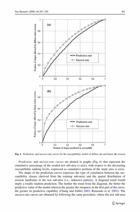
Prediction- and success-rate curves are plotted in graphs (Fig. 6) that represent the

cumulative percentage of the eroded test sub-area (y-axis), with respect to the decreasing

susceptibility ranking levels, expressed as cumulative portions of the study area (x-axis).

The shape of the prediction curves expresses the type of correlation between the sus-

ceptibility classes (derived from the training sub-area) and the spatial distribution of

erosion landforms in the test sub-area (i.e., unknown pattern). A diagonal trend would

imply a totally random prediction. The further the trend from the diagonal, the better the

predictive value of the model whereas the greater the steepness in the first part of the curve,

the greater its predictive capability (Chung and Fabbri 2003; Remondo et al. 2003). The

success-rate curves are obtained by following the same procedure, where the test sub-area

Fig. 6 Prediction- and success-rate curves for the susceptibility model of diffuse (a) and linear (b) erosion

Nat Hazards (2008) 46:287–305 301

123

is used to assess the susceptibility levels, instead of the training sub-area; these values are

then ranked so as to produce the prediction images. The success-rate curves allow us to

estimate the goodness of fit of the predictive models.

When the susceptibility assessment method or model works well, the prediction-rate

curve should fit on the success-rate curve, both having a similar monotonically decreasing

steepness.

The validation of the susceptibility models for the Naro river basin (Fig. 6) confirms an

actual (not random) correlation between the prediction images (water erosion susceptibility

maps) and the target patterns (spatial distribution of landsurfaces affected by diffuse and

linear erosion). However, some differences in the shapes of the curves (i.e., in the pre-

dictive performance of the models) arise when the water erosion landform types are taken

into consideration separately.

The results regarding the DIF landforms show (Fig. 6a) that, although neither of the two

validation curves fit the condition of a very high gradient in the first classes, more than

50% of the diffusely eroded areas fall within 40% of the most susceptible areas. Also, a

tangent monotone decreasing condition is, however, satisfied. On the other hand, both the

two curves regarding the LIN landforms show (Fig. 6b) better trends, as they increase

much more steeply than DIF-curves in the most susceptible class ranges: the prediction

curve shows that 50% of the total eroded area in the test sub-areas falls within 30% of the

most susceptible areas. Anyway, both the DIF and LIN validation curves are quite far

above the random diagonal trend (particularly the LIN-curves) and show a shift between

the success and the prediction curves (particularly the DIF-curves) smaller than the dis-

tance between the prediction curve and random trend.

4 Discussion and concluding remarks

A water erosion susceptibility assessment has been attained for the Naro river basin in

southern Sicily, by means of a geostatistical multivariate approach. The method adopted

exploits the spatial distribution of the water erosion landforms produced in the past, to

quantitatively estimate their future trend, taking into consideration, a set of interdependent

selected factors. The density of erosion landforms, computed for each of the UCUs, has

been selected as an adequate predictive function, as it actually expresses the conditional

probability for water erosion processes to affect the same UCU, wherever it occurs.

By analysing the UCUs that resulted as the most susceptible to diffuse or linear water

erosion processes (Tables 2, 3), it has been possible to evaluate the geomorphologic

relationships between each factor and the two types of processes.

As regarding to the erosivity factors, the spatial distributions of the recognized erosion

landforms agree with some general geomorphologic considerations. The landsurfaces

affected by diffuse water erosion are in fact mainly associated with slopes characterized by

a transverse moderate convexity (positive PCV values), having also limited upslope

contributing area and/or slope angle (low LSF and SPI values): these topographic condi-

tions are largely diffused in the basin, characterizing all those sectors, in which the erosive

power of the runoff water is dispersed in a parallel or diverging flow. On the contrary, the

linear erosion process is strictly associated to very concentrated water flows: it mainly

affects areas having high slope angle and/or upslope contributing area (high LSF and SPI

values), with a clearly concave topographic transverse profile (negative PCV values).

The erodibility factors have shown an expected response, for the outcropping lithology

and the soil texture, and an unexpected one for the soil use. In fact, clayey and gypseous

302 Nat Hazards (2008) 46:287–305

123

clays, with fine-medium soil textures, are the conditions more frequently associated with

both types of water erosion processes. As regarding the soil use, linear erosion does not

show any marked ‘‘preference’’ for soil uses, while, surprisingly, diffuse water erosion,

whose evidences are largely represented by landsurfaces affected by the sheet erosion

process, results to ‘‘prefer’’ lands dominated by viticulture.

The analysis of the susceptibility maps and their validation has demonstrated that the

relationships between factors and landsurfaces, above described, propagate in the predic-

tion- and success-rate curves. In fact, as the conditions for diffuse water erosion, mainly

controlled by soil use, soil texture and outcropping lithology, are largely diffused almost all

over the basin (compare Figs. 3a–c with 4a), the success- and the prediction-rate curves for

the DIF susceptibility map are not fully satisfying (Fig. 6a): they present a too smoothed

shape with a very gentle decreasing steepness; they are not so far above the random

diagonal trend. On the contrary, as the topographic factor values that mainly control the

linear water erosion susceptibility, are much more differentiated in the area (compare

Figs. 3d, e with 4b), the success and the prediction curves (Fig. 6b): draw a more convex

shape, with a more enhanced decreasing of the steepness, towards the less susceptible

classes; are located far above from the random trend. A strict correlation between the

susceptibility model and the unknown target pattern so arises for the linear water erosion

process, in the studied area.

The spatial partition strategy applied for the validation procedure has been carried out

under two main constrains: random selection of the UCU grid cells; balanced frequencies

for each single UCU in the training and the test sub-areas. Such a procedure allows to fully

satisfy a homogeneity condition for the UCUs frequency in the sub-areas, so that two real

twin areas can be produced and a faithful susceptibility value from the training area, can be

transferred to each cell in the test one. Besides, the proposed criterion is capable to

randomly produce two similar sub-areas also when a large set of controlling factors is

considered.

Actually, the method is affected by some source of errors and some subjective steps,

that must be pointed out and discussed.

Mapping errors can modify the number, the location and the geomorphologic inter-

pretation (typology) of the landform dataset. These constitute a very critical point for a

photointerpretation based mapping method (as the one proposed here), heavily depending

on the quality and scale of the aerial photos, and on the experience and coherence of the

mapping team (Ayalew et al. 2005). In order to reduce the incidence of the mapping errors,

without loosing the large advantages deriving from the aerial photo interpretation (e.g.,

synoptic and dynamic 3D view, analysis of isochronal photograms, reduced time costs),

field checking in selected test sites have been carried out to calibrate the adopted mapping

criteria. Besides, the detail of the erodibility factor maps, which can also be affected by

boundaries and characterization errors, and the resolution limits of the DEM, from which

the erosivity factors are extracted, add further inaccuracy on the susceptibility assessment.

The susceptibility assessment methods suffer from some objectivity failures mainly

arising from the interpretation of the erosion evidences, the selection of the controlling

factors and of the predictive function, the validation strategy. In the method proposed here

some devices aiming to minimize such effects have been adopted: the landsurfaces have

been grouped in only two categories; a quite large set of factors have been considered; both

the validation procedures and the susceptibility function that have been adopted are largely

accepted and applied; moreover, an automatic random partition has been performed for

validating data.

Nat Hazards (2008) 46:287–305 303

123

In conclusion, the results of the research point out that the susceptibility models defined

for diffuse and linear water erosion both satisfy a statistical proof, as they have been

successfully validated, and are coherent with geomorphologic assumptions, as they largely

fit the expected relationships between factors and processes. Moreover, the whole proce-

dure is easily exportable to other areas if source data of good accuracy are available.

A calibration of the model can be achieved by applying the susceptibility function to other

areas, having the same geoenvironmental conditions, and comparing the prediction images

to their actual landforms distribution. By the other side, an update of the landforms in the

Naro river basin would allow to test the capability of the model to reproduce also the

temporal evolution of the water erosion processes.

Acknowledgements The research, the results of which are herein described, was carried out in theframework of the national research project: MIUR PRIN COFIN 2004, national coordinator Prof. GiulianoRodolfi, local coordinator Prof. Valerio Agnesi. The suggestions of the anonymous referees have reallygiven the authors the opportunity for enhancing the completeness and the scientific clearness and rigour ofthe article. Authors wish to thank Dr Penelope Dyer for performing the linguistic revision of the text.

References

Agnesi V, Cappadonia C, Conoscenti C, Di Maggio C, Marker M, Rotigliano E (2006) Valutazionedell’erosione del suolo nel bacino del Fiume San Leonardo (Sicilia Centro-Occidentale, Italia). In:Rodolfi G (ed) Atti del Convegno Conclusivo del Progetto MIUR-COFIN 2002 Erosione idrica inambiente mediterraneo: valutazione diretta e indiretta in aree sperimentali e bacini idrografici, Firenze2004, 13–27

A.R.T.A. Sicilia (1994a) Carta dell’Uso del Suolo (scala 1:250000). Assessorato Territorio ed Ambientedella Regione Sicilia, Palermo

A.R.T.A. Sicilia (1994b) Sezioni 637140, 637130, 637100, 637090, 637070, 637060, 637050, 637030,637020, 637010, 636160, 636120, 636080. Assessorato Territorio ed Ambiente della Regione Sicilia,Palermo

Ayalew L, Yamagishi H, Marui H, Kanno T (2005) Landslides in Sado island of Japan: part II. GIS-basedsusceptibility mapping with comparisons of results from two methods and verifications. Eng Geol81:432–445

Carrara A, Guzzetti F (eds) (1995) Geographical information systems in assessing natural hazards. KluwerAcademic Publishers, Dordrecht

Catalano R, Di Stefano P, Nigro F, Vitale FP (1993) Sicily mainland and its offshore: a structural com-parison. In: Max MD, Colantoni P (eds) Geological development of the Sicilian–Tunisian platform,UNESCO Report in Marine Science, 58:19–24

Chung CF, Fabbri AG (2003) Validation of spatial prediction models for landslide hazard mapping. NatHazards 30:451–472

Ciccacci S, Fredi P, Lupia Palmieri E, Pugliese F (1981) Contributo dell’analisi geomorfica quantitativa allavalutazione dell’entita dell’erosione nei bacini fluviali. Boll Soc Geol It 99:455–516

Conoscenti C, Di Maggio C, Rotigliano E (2006) Analisi mediante GIS dei processi di erosione nel bacinodel Fiume Naro (Sicilia Centro-Meridionale, Italia). In: Rodolfi G (ed) Atti del Convegno Conclusivodel Progetto MIUR-COFIN 2002 Erosione idrica in ambiente mediterraneo: valutazione diretta eindiretta in aree sperimentali e bacini idrografici, Firenze 2004, 211–227

Conoscenti C, Di Maggio C, Rotigliano E (2007) GIS analysis to assess landslide susceptibility in a fluvialbasin of NW Sicily (Italy). Geomorphology. doi:10.1016/j.geomorph.2006.10.039

Ferro V, Giordano G, Iovino M (1991) Isoerosivity and erosion risk map for Sicily. J Hydrol Sci 36(6):549–564

Fierotti G (1988) Carta dei Suoli della Sicilia. Ist. di Agronomia, Univ. di Palermo e Regione Sicilia,Assessorato Territorio ed Ambiente, Palermo

Marker M, Flugel WA, Rodolfi G (1999) Das Konzept der ‘‘Erosions Response Units’’ (ERU) und seineAnwendung am Beispiel des semi-ariden Mkomazi-Einzugsgebietes in der Provinz Kwazulu/Natal,Sudafrika. In: Tubinger Geowissenschaftliche Studien, Reihe D.: Geookologie und Quartaerforschung.Angewandte Studien zu Massenverlagerungen, Tubingen

304 Nat Hazards (2008) 46:287–305

123

Moore ID, Grayson RB, Ladson AR (1991) Digital terrain modeling: a review of hydrological, geomor-phological, and biological applications. Hydrol process 5:3–30

Nearing MA, Foster GR, Lane LJ, Finkner SC (1989) A process-based soil erosion model for USDA-watererosion prediction project technology. Trans Am Soc Agric Eng 32:1587–1593

O’Callaghan JF, Mark DM (1984) The extraction of drainage network from digital elevation data. ComputVis Graph Image Process 28:323–344

Regione Siciliana (1955) Carta Geologica d’Italia, Foglio 271, Agrigento, scala 1:100.000Remondo J, Gonzalez-Diez A, Diaz De Teran JR, Cendrero A (2003) Landslide susceptibility models

utilising spatial data analysis techniques. A case study from the lower Deba Valley, Guipuzcoa (Spain).Nat Hazards 30:67–279

Renard KG, Foster GR, Weesies GA, Mccool DK, Yoder DC (1997) Predicting soil erosion by water:a guide to conservation planning with the Revised Universal Soil Loss Equation (RUSLE). USDA Agr.Res. Serv. Handbook n. 703

Servizio Geologico Italiano (1972) Carta Geologica d’Italia, Foglio 635, Agrigento, scala 1:50.000Wilson JP, Gallant JC (2000) Terrain analysis: principles and applications. Wiley & Sons, Inc., CanadaWischmeier WH, Smith DD (1965) Predicting rainfall erosion losses from cropland east of Rocky Moun-

tains; guide for the selection of practices for soil and water conservation. Agriculture handbook n. 282,Agr. Res. Serv. in Coop. Purdue Agr. Exp. Station US Dept. of Agr., Washington

Nat Hazards (2008) 46:287–305 305

123