Engineering Geology 205 (2016) 93–103

Contents lists available at ScienceDirect

Engineering Geology

j ourna l homepage: www.e lsev ie r .com/ locate /enggeo

Geostatistical simulation to map the spatial heterogeneity ofgeomechanical parameters: A case study with rock mass rating

Marisa Pinheiro a,⁎, Javier Vallejos b,c, Tiago Miranda a, Xavier Emery b,c

a ISISE, University of Minho, Azurém, 4800-058 Guimarães, Portugalb Department of Mining Engineering, University of Chile, Avenida Tupper, 2069 Santiago, Chilec Advanced Mining Technology Center, University of Chile, Avenida Beauchef, 850, Santiago, Chile

⁎ Corresponding author.E-mail address: marisamotapinheiro@gmail.com (M. P

http://dx.doi.org/10.1016/j.enggeo.2016.03.0030013-7952/© 2016 Elsevier B.V. All rights reserved.

a b s t r a c t

a r t i c l e i n f o

Article history:Received 1 August 2015Received in revised form 8 March 2016Accepted 14 March 2016Available online 17 March 2016

A better characterization of complex rock masses is essential in geotechnical engineering, as the empirical sys-temswidely used for this purpose have significant limitations and do not provide adequate answers for risk anal-ysis. Geostatistics offers a set of tools that allow not only predicting the rock mass properties, but also mappingtheir heterogeneity at different spatial scales and quantifying the uncertainty in their actual values. In thispaper, two geostatistical approaches are compared for modeling the Rock Mass Rating (RMR), which is used togeomechanically characterize the rock mass in geotechnical works. The first approach consists of the direct sim-ulation of the RMR values, based on a Gaussian spatial random fieldmodel. In contrast, the second approach usesthe truncated Gaussian model to separately simulate the individual parameters of the RMR, which subsequentlyare summed to obtain the final RMR value. The computation time, practical implementation, level of details andpost-processing outputs that can be obtained from both approaches are analyzed. Besides the RMRmapping andassociated uncertainty, the deformation modulus is subsequently obtained based on these maps together withempirical expressions.

© 2016 Elsevier B.V. All rights reserved.

Keywords:Rock Mass RatingRock mechanicsGeostatistical simulationSpatial heterogeneitySpatial uncertainty

1. Introduction

In the current practice of geotechnical works design, thegeomechanical parameters of the rock formations are set based on cam-paigns of in situ and laboratory characterization works and tests. Ac-cording to the results of these campaigns, a geotechnical zoning isestablished and a set of geomechanical parameters is assigned to eachzone. This is a highly subjective exercise, but its output is of utmost im-portance for the next stages of geotechnical design. However, this ap-proach does not properly account for the intrinsic spatial variabilityand high heterogeneities that can be found in many rock masses,which can have a significant impact on the structure behavior. In thissense, there is a lack of an approach that allows reducing the subjectivityof geotechnical zoning and that explicitly considers the spatial variabil-ity and heterogeneities many times present in rock masses.

The recourse to geostatistical models can be a mean to foster thedevelopment of such an approach. Indeed, in these models, thegeomechanical parameters are viewed as outcomes (realizations) of spa-tial random fields, the properties of which can be inferred from the avail-able in situ measurements and laboratory tests. Kriging techniques(Matheron, 1971) can be used to predict the values of the parameters ofinterest at any specific location, based on the information available at

inheiro).

neighboring locations and on the spatial correlation structure of the un-derlying random fields. These techniques aim to minimize the expectedsquared error between predicted and true values, but, in return, they pro-vide over-smoothed maps that do not reflect the actual variability of thetrue parameters. To avoid this drawback, conditional simulation tech-niques have been developed to construct numerical models that repro-duce the spatial variability at all scales and allow a better understandingof the rock mass heterogeneities (Journel, 1974; Chilès and Delfiner,2012). Unlike kriging that provides a single prediction for each parameterof interest, simulation yields asmany case scenarios as desired, which arehelpful to assess the uncertainty in the actual (unknown) parametervalues at any specific location or jointly over several locations.

Numerous authors already applied geostatistics to estimate or to simu-late properties such as lithology faces (Rosenbaum et al., 1997), Rock Qual-ity Designation (RQD) (Esfahani and Asghari, 2013; Ozturk and Simdi,2014; Ozturk and Nasuf, 2002), Rock Mass Rating (RMR) (Ryu et al.,2003; You, 2003; Oh et al., 2004; Stavropoulou et al., 2007; Exadaktylosand Stavropoulou, 2008; Jeon et al., 2009; Egaña and Ortiz, 2013; Ferrariet al., 2014), joint frequency (Ellefmo and Eidsvik, 2009) or GeologicalStrength Index (GSI) (Ozturk and Simdi, 2014; Deisman et al., 2013).

Hereunder, the system used for simulation is the Rock Mass Rating(RMR) proposed by Bieniawski (1989). This system allows classifyingthe rock mass in five classes (very good, good, fair, poor, very poor)using a continuous scale that varies from 0 to 100 obtained afterweighting six individual parameters regarding the rock mass and its

94 M. Pinheiro et al. / Engineering Geology 205 (2016) 93–103

discontinuities. The referred parameters are: a) Uniaxial compressivestrength of rock material (P1); b) RQD (P2); c) Discontinuity spacing(P3); d) Condition of discontinuities (P4); e) Groundwater conditions(P5); f) Orientation of discontinuities (P6). In this work, the sixth pa-rameter (P6) will not be used because it does not depend only on thecharacteristics of the rock discontinuities but also on their relationwith the structure and this is unknown. The RMR under considerationis therefore the so-called basic RMR, which is obtained consideringonly the contribution of parameters P1 to P5.

The next section presents two geostatistical approaches to simulatethe RMR, depending on whether one considers that the properties aremeasured on a continuous quantitative scale or on a discrete scale. Inthefirst approach, themost straightforward andusual one, RMR is viewedas a variablemeasured on a continuous scale (from0 to100) and is direct-ly simulated with a multivariate Gaussian algorithm. In contrast, the sec-ond approach ismore complete, as each one of the five parameters (P1 toP5) is simulated and the results are then summed to obtain thefinalmap-ping of RMR. A novelty of this second approach with respect to previousworks is the fact that the underlying parameters are considered as vari-ables measured on a discrete scale, which better suits their nature as aranking and not as a continuous value, and that a specific geostatisticalmodel (truncated Gaussian model) is used for the purpose of simulation.In Section 3, both approaches are applied to a case study and compared interms of implementation facility, accuracy and level of detail provided insimulating the spatial distribution of RMR. Finally the simulated RMR isconverted into deformation modulus (Em) using empirical formulae.

2. Geostatistical simulation of RMR

2.1. First approach: direct simulation of RMR

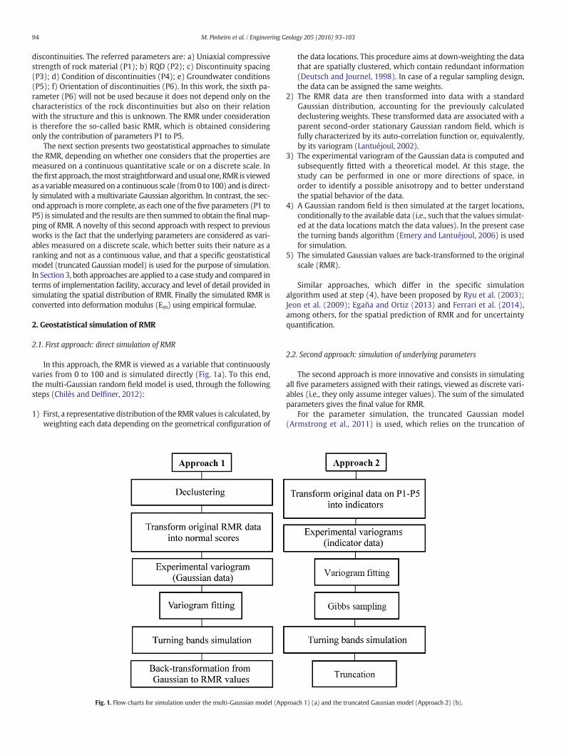
In this approach, the RMR is viewed as a variable that continuouslyvaries from 0 to 100 and is simulated directly (Fig. 1a). To this end,the multi-Gaussian random field model is used, through the followingsteps (Chilès and Delfiner, 2012):

1) First, a representative distribution of the RMR values is calculated, byweighting each data depending on the geometrical configuration of

Fig. 1. Flow charts for simulation under the multi-Gaussian model (Ap

the data locations. This procedure aims at down-weighting the datathat are spatially clustered, which contain redundant information(Deutsch and Journel, 1998). In case of a regular sampling design,the data can be assigned the same weights.

2) The RMR data are then transformed into data with a standardGaussian distribution, accounting for the previously calculateddeclustering weights. These transformed data are associated with aparent second-order stationary Gaussian random field, which isfully characterized by its auto-correlation function or, equivalently,by its variogram (Lantuéjoul, 2002).

3) The experimental variogram of the Gaussian data is computed andsubsequently fitted with a theoretical model. At this stage, thestudy can be performed in one or more directions of space, inorder to identify a possible anisotropy and to better understandthe spatial behavior of the data.

4) A Gaussian random field is then simulated at the target locations,conditionally to the available data (i.e., such that the values simulat-ed at the data locations match the data values). In the present casethe turning bands algorithm (Emery and Lantuéjoul, 2006) is usedfor simulation.

5) The simulated Gaussian values are back-transformed to the originalscale (RMR).

Similar approaches, which differ in the specific simulationalgorithm used at step (4), have been proposed by Ryu et al. (2003);Jeon et al. (2009); Egaña and Ortiz (2013) and Ferrari et al. (2014),among others, for the spatial prediction of RMR and for uncertaintyquantification.

2.2. Second approach: simulation of underlying parameters

The second approach is more innovative and consists in simulatingall five parameters assigned with their ratings, viewed as discrete vari-ables (i.e., they only assume integer values). The sum of the simulatedparameters gives the final value for RMR.

For the parameter simulation, the truncated Gaussian model(Armstrong et al., 2011) is used, which relies on the truncation of

proach 1) (a) and the truncated Gaussian model (Approach 2) (b).

95M. Pinheiro et al. / Engineering Geology 205 (2016) 93–103

second-order stationary Gaussian random fields. The application of thismodel is carried out through the following steps (Fig. 1b):

1) First, the original data are transformed into class-indicator data,i.e., data that take the value 0 or 1 depending on each parameterscore.

2) For each individual parameter, a set of truncation thresholds is de-fined, which allows the proportion of each class to be reproducedby the simulation (Armstrong et al., 2011).

3) Given the experimental variograms of the class-indicator data, avariogram can be calculated for the underlying Gaussian randomfield associated with each parameter, based on the existing relation-ships between the indicator and Gaussian variograms (Emery andCornejo, 2010). The Gaussian variograms so obtained can be fittedwith theoretical models.

4) The class-indicator data are then transformed into simulated Gauss-ian data, using an iterative algorithm known as the Gibbs sampler(Armstrong et al., 2011; Lantuéjoul, 2002).

5) The Gaussian random fields are simulated at the target locations,conditionally to the Gaussian values obtained at the previous step,and are truncated in order to get back to simulated class-indicatorvalues. As for the first approach, the turning bands algorithm isused for the simulation of Gaussian fields.

6) The indicators are converted into the underlying parameters andfinally into RMR values.

3. Case study

The two previous approaches are now applied to a case study inorder to map the RMR in an epithermal gold deposit located in the“Cordillera de Los Andes”, region of Atacama, northern Chile, and sur-veyed through a set of exploration boreholes. The regional geology ofthe area is characterized by a group of intrusive, volcanic and sedimen-tary rocks, affected by fault zones that control the mineralization,allowing the identification of fourmain lithological units of sedimentaryrocks.

The available data comprise 3969 samples obtained from boreholeswith a horizontal spacing of 40 m × 40 m and depths rangingfrom 96 m to 390 m. Along these boreholes, the samples are takenwith a spacing of 20 m, yielding a regular sampling design of40m × 40m × 20m. The uniaxial compressive strength (P1) wasmea-sured from laboratory tests. Cylindrical rock samples were prepared ac-cording to the standard ASTM D4543–08, and then tested underuniaxial compressive conditions using the standards included in ASTMD7012–04. The average prepared sample has an aspect ratio (H/D) of2. Table 1 presents the average density and the uniaxial compressivestrength normalized to a diameter of 50 mm (UCS50 mm) for each litho-logical unit. TheRQD (P2)was estimated directly fromborehole logging.To estimate the average discontinuity spacing (P3), the average fre-quency of fractures (FF/m) was estimated. Bias correction was then ap-plied by considering the average angle of each measured discontinuity.The condition of discontinuities (P4) was not quantitatively measuredat the field. A regular condition was assumed for all lithological units.Finally, the water condition (P5) was assigned in agreement to thelevel of water determined at different depths at each borehole; twoclasses were mainly identified: wet and damp.

Table 1Information about average UCS and average density by lithological unit.

Lithological unit Description

Silty and clayey limestone Medium to fine calcareous sandstone and limestoneCalcareous sandstone Fine bioclastic calcareous sandstones, limestones and bioclaSandstone Calcareous sandstone with rounded fragments of quartzCalcareous sandstone Sandstones with interblended limestones; levels of fine mu

According to the results of rock mechanics laboratory tests and theinterpreted RMR values from the borehole samples, the rock mass isclassified with a quality of fair to good (mostly in the range of 50 to60). This range of RMR values is used in the mine design process. Planviews of the data are shown in Fig. 2.

The RMR simulation should result in a better and improved under-standing of the spatial distribution and an easier identification of het-erogeneities and uncertainty levels. In addition to RMR, the underlyinggeomechanical parameters (P1 to P5) could also be mapped and conse-quently used in numerical models and mine design process in order toobtain a more accurate zoning of the rock mass.

3.1. Exploratory analysis

Basic statistics of the data are presented in Table 2. RMR may varyfrom 0 to 100, while the values of the parameters P1 to P5 refer totheir rating obtained from the application of the RMR system.

According to the data statistics, with a minimum RMR value of 48and a maximum value of 78, the geomechanical quality of the rockmass varies from fair to good. Concerning the individual parameters(Fig. 3), P1 varies within a short range, meaning that the UCS of the in-tact rock is almost constant, unlike P2 and P3 that vary in a muchwiderrange showing very different levels of rock mass fracturing. In contrast,for all the samples, the fourth parameter (P4) is constant and equal to20. This parameter is related to the condition of the discontinuities, sothey are all classified as having slightly rough surfaces with a separationsmaller than 1 mm and a highly weathered wall rock. Accordingly, thesame score (20) will be assumed for all the points of the target simula-tion grid. Lastly, like P1, parameter P5 varies within a short range, withonly two different scores, representing a groundwater condition that ismostly wet (7) and punctually damp (10).

Before performing the simulation of parameters P1, P2, P3 and P5, itis necessary to observe the existing correlations between them, in orderto make sure that they are not (or weakly) cross-correlated. Otherwise,the separate parameter simulation in the second approach should be re-placed by co-simulation,whichwouldmake themodel quitemore com-plex (Emery and Cornejo, 2010). The correlationmatrix, which containsthe Pearson product–moment correlation coefficients between all theparameters, is presented in Table 3. Analyzing these coefficients, one ob-serves that the only parameterswith a positive correlation are P3 and P5comparatively to P2, whereas the others parameters show a slightlynegative correlation between them. However, these correlations arerather weak from a statistical point of view (less than 0.3 in absolutevalue), so that the information on a parameter actually brings little in-formation on the other parameters. The low correlation between P2(RQD) and P3 (discontinuity spacing) can be explained by the goodquality of the rockmass, which translates into a wide spacing of the dis-continuities and high RQD values, making the latter parameter less sen-sitive to closer discontinuities. As such, in Approach 2 the simulation ofthe four RMRparameters can be performed separately as individual var-iables; co-simulation, which enhances the simulation of a set of vari-ables in order to reproduce their cross-correlation, is not necessary here.

3.2. Modeling univariate distributions

As previously mentioned, for the first approach, the data should betransformed into normal scores. Since the sampling design is regular,

Average density (t/m3) Average UCS (MPa)

2.68 ± 0.05 215 ± 56stic clams 2.68 ± 0.09 154 ± 47

2.64 ± 0.02 143 ± 20lticolored calcareous sandstones 2.63 ± 0.06 152 ± 40

Fig. 2. 2D maps of spatial distribution at elevation 3560 m, for RMR original values (a), Parameter P2 (b) and Parameter P3 (c).

96 M. Pinheiro et al. / Engineering Geology 205 (2016) 93–103

there is no need for declustering, i.e., all the data are assigned the sameweighting. The function that relates the original RMR values and the as-sociated Gaussian values (anamorphosis function) can then be calculat-ed empiricallywith the available data. This function ismodeled by usinga piecewise linear interpolation between the empirical points, and ex-ponential functions for tail extrapolation, as explained in Emery andLantuéjoul (2006) (Fig. 4). The parameters of these exponential func-tions are chosen in order tofit amodel as continuous as possible. The ab-solute minimum and maximum values for RMR are set to 45 and 80,respectively.

Regarding Approach 2, the data related to Parameter 1 only presenttwo different scores, 12 and 14, with relative proportions of 0.468 and0.532, respectively. This distribution can be modeled by truncating astandard normal distribution, using a single truncation threshold setto G−1(0.468) = −0.0803, with G the standard normal cumulativedistribution function. In other words, the probability for a standardGaussian random variable to be less than −0.0803 is 0.468, and theprobability to be more than −0.0803 is 0.532, coinciding with the pro-portions of the two scores of Parameter 1. Likewise, the data of Param-eter 5 only assume two different scores, 7 and 10, with relativeproportions of 0.989 and 0.011, respectively. Again, the model uses asingle truncation threshold, here equal to G−1(0.989) = 2.2904.

In a different way, the data of Parameters 2 and 3 assume almostevery score. As a result, a larger number of truncation thresholds haveto be defined, as shown in Tables 4 and 5, respectively. These truncationthresholds are such that the proportion of data with a given score coin-cideswith the probability for a standard Gaussian random variable to bebetween the lower and upper thresholds associated with this score.

3.3. Modeling spatial continuity: variogram analysis

For both approaches, following the methodology explained inSection 2, the variograms of the Gaussian random fields to simulate

Table 2Basic statistics on RMR ratings and original data (3969 samples).

RMR P1 (UCS) P2 (RQD)

Rating MPa Rating %

Minimum 48.0 12.0 138.0 3.0 0.0Maximum 78.0 14.0 208.0 20.0 100.0Mean 66.7 13.1 177.8 16.4 87.3Standard deviation 3.8 1.0 32.5 2.7 12.3

a 1.0 was the value used to represent the intermediate rating of the joint condition.b 1.0 and 2.0 represent a groundwater condition of Wet and Damp, respectively.

have to be calculated along the main directions of anisotropy. Becauseof the sampling design (vertical boreholes), it is not possible to experi-mentally calculate variograms in inclined directions, thus calculationsare restricted to the vertical direction and to the horizontal plane. Fur-thermore, isotropic variograms are calculated on this plane, insofar asno clear anisotropy is detected in the experimental variograms associat-ed with different horizontal directions. For calculations, the lag dis-tances are multiple of 20 m along the vertical, which corresponds tothe data spacing along the boreholes, and of 40 m along the horizontal(borehole spacing), with a tolerance of 20 m.

The experimental variograms (hereafter denotedwith the Greek let-ter γ) so calculated are then fitted using combinations of basic nestedstructures (exponential, spherical, cubic and Gaussian, see Chilès andDelfiner, 2012 for details on these basic models), as follows.

• Variogram model for Approach 1 (normal score transform of RMR):

γ ¼ 0:771 Exponential 250 m;250 mð Þþ 0:305 Gaussian 450 m;250 mð Þ

• Variogram models for Approach 2:

P1 : γ1 ¼ 1 Cubic 700 m;100 mð Þ

P2 : γ2 ¼ 1 Exponential 350 m;300 mð Þ

P3 : γ3 ¼ 0:639 Exponential 300 m;250 mð Þþ 0:361 Gaussian 300 m;350 mð Þ

P5 : γ5 ¼ 0:01 Exponential 30 m;∞ð Þ þ 0:99 Gaussian 700 m;150 mð Þ:

P3 (JS) P4 (JC) P5 (GW)

Rating mm Rating JC Rating GW

5.0 23.0 20.0 1.0a 7.0 1.0b

19.0 1923.0 20.0 1.0a 10.0 2.0b

10.2 220.5 20.0 1.0a 7.0 1.02.0 170.2 0.0 0.0 0.3 0.1

Fig. 3. Data histograms for Parameters P1 (a), P2 (b), P3 (c) and P5 (d).

97M. Pinheiro et al. / Engineering Geology 205 (2016) 93–103

In the above equations, the coefficient preceding a basic nestedstructure indicates the sill of this structure (contribution to the totalvariance), while the distances written between brackets represent thecorrelation ranges of the structure along the horizontal plane and thevertical direction, respectively. The experimental and theoreticalvariograms for Approaches 1 and 2 are shown in Figs. 5 and 6, respec-tively. It should be noticed that none of the variograms exhibit a nuggeteffect (discontinuity near the origin), indicating that the RMR and itsunderlying parameters are continuous in space. Even more, thevariogrammodels for P1 and P5 have a smooth behavior near the originand a large correlation range along the horizontal direction (700 m),which indicates that the regions where these parameters are constanthave smooth boundaries and a large spatial extent or spatial connectiv-ity (recall that both P1 and P5 only assume two different scores).

3.4. Conditional simulation results

The model parameters being specified (anamorphosis function inApproach 1, truncation thresholds in Approach 2, and variograms ofthe underlying Gaussian random fields in both approaches), conditionalrealizations of the RMR and of the underlying parameters can be con-structed. In this work, adaptations of previously published computer

Table 3Correlation matrix between parameters P1, P2, P3 and P5.

P1 P2 P3 P5

P1 1 −0.096 −0.164 −0.113P2 −0.096 1 0.292 0.045P3 −0.164 0.292 1 −0.032P5 −0.113 0.045 −0.032 1

programs are used for simulating Gaussian and truncated Gaussian ran-dom fields (Emery and Lantuéjoul, 2006; Emery, 2007). The number ofrealizations is set to one hundred, so that the post-processing outputs(average and conditional probabilities) could be calculated with a rea-sonable approximation. In both cases, the turningbands algorithm is ap-plied with 1000 turning lines to generate the Gaussian random fields,and simple kriging is used to condition the realizations to the boreholedata. For Approach 2, the Gibbs sampler is stopped after one hundred

Fig. 4. Anamorphosis function used for Approach 1. The ordinate indicates the RMR valueand the abscissa the associated Gaussian value.

Table 4Calculated proportions for P2 data with the corresponding Gaussian thresholds.

Score for P2 Cumulative proportion Lower threshold Upper threshold

1 0 −∞ −∞2 0 −∞ −∞3 0.0033 −∞ −2.71644 0.0043 −2.7164 −2.62765 0.0073 −2.6276 −2.44226 0.0080 −2.4422 −2.40897 0.0150 −2.4089 −2.17018 0.0200 −2.1701 −2.05379 0.0250 −2.0537 −1.960010 0.0360 −1.9600 −1.799111 0.0510 −1.7991 −1.635212 0.0780 −1.6352 −1.418713 0.1120 −1.4187 −1.216014 0.1710 −1.2160 −0.950215 0.2710 −0.9502 −0.609816 0.4520 −0.6098 −0.120617 0.6200 −0.1206 0.305518 0.8180 0.3055 0.907819 0.9900 0.9078 2.326320 1.0000 2.3263 +∞ Fig. 5. Experimental (crosses) and theoretical (solid lines) variograms for RMR (Approach

1) along the main anisotropy directions: horizontal (black) and vertical (blue).

98 M. Pinheiro et al. / Engineering Geology 205 (2016) 93–103

iterations and the simulated Gaussian random fields are truncated,based on the thresholds indicated in Section 3.2 and Tables 4 and 5,yielding realizations of parameters P1 to P5 that are subsequentlysummed to obtain realizations of the RMR values.

For ease of display, the locations targeted for simulation correspondto a regular two-dimensional grid placed at elevation 3560 m, with amesh of 5 m × 5 m and a total of 160 nodes along the east directionand 240 nodes along the north direction.

The average of the RMR realizations is calculated tomap the expect-ed RMR over the region of interest resulting from both approaches(Fig. 7b, e). Furthermore, in order to demonstrate the spatial variabilityexisting in this rock mass, the first realization is mapped as an example(Fig. 7a, d). In these figures, the neighboring data values aresuperimposed on the maps in order to highlight the effect of condition-ing the RMR realizations to the borehole data: when a target grid nodecoincideswith a data location, the simulated RMRvalue exactlymatchesthe conditioning data value.

The visual comparison suggests that the two approaches producesimilar results for RMR. It is worth noticing that the map of the realiza-tion average tends to smudge the contrasts and that spatial heterogene-ities appear as much more faded. The analysis of the individualrealizations is therefore important to visualize the real heterogeneity

Table 5Calculated proportions for P3 with the corresponding Gaussian thresholds.

Score for P3 Cumulative proportion Lower threshold Upper threshold

1 0 −∞ −∞2 0 −∞ −∞3 0 −∞ −∞4 0 −∞ −∞5 0.0500 −∞ −1.64496 0.0501 −1.6449 −1.64397 0.0502 −1.6439 −1.64298 0.1842 −1.6429 −0.89959 0.3432 −0.8995 −0.403710 0.5422 −0.4037 0.106011 0.8152 0.1060 0.897212 0.9182 0.8972 1.393113 0.9582 1.3931 1.730214 0.9762 1.7302 1.980915 0.9872 1.9809 2.232216 0.9912 2.2322 2.373917 0.9952 2.3739 2.589918 0.9998 2.5899 3.540119 1.0000 3.5401 +∞20 1.0000 +∞ +∞

that it is expected to be observed in the field, whereas the average ofthe realizations shows an overall trend, which is much smoother.

3.5. Post-processing simulations

More outputs can be represented, like the probability that the RMRexceeds or falls short of a predefined value, which can be estimated bythe frequency of threshold exceedance or non-exceedance observedover the realizations. This representation is of great value if one wantsto identify regions where very high or low geomechanical propertiescould be present, and with which probability. As an example, for bothapproaches, Fig. 8 shows the map of the probability that the actualRMR is less than a threshold of 65.

Fig. 9 (a, b, d, e) shows themaps of parameters P2 and P3 for the firstrealization and for the average of 100 realizations obtained with Ap-proach 2, which helps to visualize the spatial distribution and variabilityof the discontinuity parameters. Comparing realization #1 with theaverage of 100 realizations for both parameters, the pattern in loweror higher rating are similar, however, as already referred, the averagemapping exhibits smoother values. The individual analysis of the dis-continuity parameters can, by itself, result in a powerful tool in geotech-nical works to understand the regionswhere the rockmass can bemoreor less fractured. Attentively, comparing the P2 and P3 maps (averageand first realization), it is possible to identify a small region in thewest-ern part of the grid, with low values of RQD (P2) and intermediatevalues of the discontinuity spacing (P3). These incoherent values are ac-tually present in the borehole data used for conditioning the realiza-tions, therefore they are not a problem of the proposed simulationapproach, but rather a problem of the input data. This could be ex-plained by human errors in the measurement of parameter P2.

Maps of other geomechanical parameters can be obtained based onthe realizations of RMR. In this work, considering that the RMR valuesare higher than 50, the distribution maps of the deformation modulus(Em) were developed with the Bieniawski (1978) empirical formula:

Em ¼ 2� RMR−100:

This formula uses the simulated values of RMR to obtain the Emvalues at the same locations. Alike the maps computed for the RMRvalues, Fig. 10 (a, b) shows the average of Em obtained from the 100 con-ditional realizations of Approach 1, as well as the first realization, as an

Fig. 6. Experimental (crosses) and theoretical (solid lines) variograms for Approach 2 along the main anisotropy directions: horizontal (black) and vertical (blue): Parameters P1 (a), P2(b), P3 (c) and P5 (d).

99M. Pinheiro et al. / Engineering Geology 205 (2016) 93–103

example. With this map it is possible to distinguish zones where therock mass is significantly stiffer and zones with lower rigidity.

Finally, to visualize the uncertainty in the true values, the standarddeviation (or any other uncertainty measure, such as the coefficient ofvariation or the limits for a given level of confidence) can be calculatedat each target node over the 100 realizations and mapped throughoutthe grid of interest. As an example, the standard deviations of RMR ob-tained with both approaches, of parameters P2 and P3 obtained in thetruncated Gaussian model (Approach 2) and of the deformation modu-lus Em obtained in the multi-Gaussian model (Approach 1) are mappedin Fig. 7 (c, f), Fig. 9 (c, f) and Fig. 10 (c), respectively. Suchmaps indicatehowmuch the true unknown values are likely to deviate from their ex-pected values (averages of the realizations) at each target grid node,therefore quantify the local uncertainty in the true values. The mappedstandard deviations depend on the number and location of the sur-rounding borehole data (they increase in under-sampled areas and pe-ripheral areas without data) and, to a lesser extent, on the parametervalues: for P3, whose distribution is positively skewed, the standarddeviation tends to increase in high-valued areas, while the reverse hap-pens for RMR, P2 and Em whose distributions are negatively skewed, aphenomenon known as proportional effect (Manchuk et al., 2009) or re-gressive effect (David, 1988). Furthermore, the maximum standard de-viation for RMR occurs in the north-western side of the grid of interestand is about 7 (Fig. 7), which represents a small deviation for a variablethat varies from 0 to 100. This suggests a relatively low uncertainty inthe true RMR values at unsampled locations.

The standard deviations mapped in Figs. 7, 9 and 10 should not beconfused with the ones presented in Table 2: the former measure thevariability across the realizations at a given location, therefore dependon the location under consideration, whereas the latter measure the

variability of a data set across the region of interest, withoutdistinguishing any specific location.

3.6. Split-sample cross-validation

To validate the two approaches the original data set is randomly di-vided into two subsets, each containing one half of the data. Thereby,thefirst subset (training subset) is used to simulate the RMR at the loca-tions of the data belonging to the second subset (validation subset).

In order to validate the prediction capability of both approaches, theexpected RMR, calculated as the average of the simulated RMR values, iscompared with the real values at the locations of the validation subset(Fig. 11a, b). To analyze the results, a linear regression and the coeffi-cient of determination between expected and true RMR values are cal-culated. For both approaches, the resulting points of the scatter plotare distributed close to the diagonal line and the coefficient of determi-nation is high (0.788 and 0.771, respectively, for Approaches 1 and 2).This indicates that the simulations allow an accurate prediction ofRMR, with small error fluctuation and no conditional bias (Chilès andDelfiner, 2012). Accuracy can be confirmed by calculating the RootMean Squared Error (RMSE):

RMSE ¼

ffiffiffiffiffiffiffiffiffiffiffiffiffiffiffiffiffiffiffiffiffiffiffiffiffiffiffiffiffiffiffiffiXN

i¼1yi−yi

� �2N

sð1Þ

where N denotes the number of data in the validation subset, yi the truevalue and yi the expected value (average of the realizations). The RMSEvalues are 1.74 for Approach 1 and 1.81 for Approach 2. Since RMRvaries from 0 to 100, an error less than 2 is almost residual.

Fig. 7.Maps of RMR at elevation 3560 m, for realization #1 (a, d), average of 100 realizations (b, e), standard deviation of 100 realizations (c, f), obtained with Approach 1 (a, b, c) andApproach 2 (d, e, f).

100 M. Pinheiro et al. / Engineering Geology 205 (2016) 93–103

In order to validate the capability of modeling uncertainty, accuracyplots (Goovaerts, 2001) are constructed. In these plots, one considers agiven probability p and, based on the obtained realizations, one can de-fine at each target location an intervalwith such a probability (the inter-val bounds are the quantiles 1-p/2 and 1 + p/2 of the set of simulatedvalues). Subsequently, the location is assigned a value of 1 if the trueRMR belongs to the interval and 0 otherwise. It is expected that, on av-erage over all the locations of the validation subset, the proportion of 1should be close to the probability p under consideration. This procedurehas been applied with p varying from 0 to 1 (Fig. 11c, d). In both

Fig. 8.Maps of probability (between 0 and 1) that the RMR is less than a threshold

approaches, the observed proportion is close to the theoretical probabil-ity (points close to the diagonal line, with a slightly better coincidencefor Approach 2), indicating that the realizations accurately assess theuncertainty in the actual RMR values.

3.7. Discussion

Both simulation approaches give an insight into two characteristicsof the geomechanical parameters of interest: (1) their heterogeneityat all spatial scales, especially at short scale, which can be assessed on

of 65 at elevation 3560 m, obtained with Approach 1 (a) and Approach 2 (b).

Fig. 9.Maps of discontinuity parameters at elevation 3560m, for realization#1 of P2 (a), average of 100 realizations of P2 (b), standarddeviation of 100 realizations of P2 (c), realization#1of P3 (d), average of 100 realizations of P3 (e), and standard deviation of 100 realizations of P3 (f).

101M. Pinheiro et al. / Engineering Geology 205 (2016) 93–103

each individual realization; and (2) the uncertainty in the true values atunsampled locations. The latter can be assessed by comparing a set ofrealizations at the same location or jointly over several locations,e.g., by calculating the standard deviation of the realizations at eachlocation, which measures howmuch the true unknown values may de-viate from their expected values (average of the realizations).

There are several differences between these two proposed ap-proaches, mainly regarding pre and post processing. While Approach1 allows directly simulating the RMR as a continuous variable, the quan-tity and detail of the geomechanical information is more limited whencomparedwithApproach 2 that allows the simulation of the parameters

Fig. 10.Maps of deformationmodulus (GPa) at elevation 3560m, for realization #1 (a), average1.

underlying the definition of RMR. Also, the difference in modeling andcomputational efforts for both approaches is substantial, Approach 1being a faster and simpler alternative than Approach 2. Regarding theresults, the observed differences are generally not significantwhenmap-ping one realization or the average of a set of realizations, but differencesare perceptible when mapping the standard deviations of the realiza-tions: Approach 2 yields a lower standard deviation (reflecting lessuncertainty) than Approach 1 in the peripheral zones. All things consid-ered, the choice of the best approach should be made based on the re-sources and needs of the practitioner (degree of required geotechnicaldetail, understanding of the models, software and time availability).

of 100 realizations (b), standard deviation of 100 realizations (c), obtainedwith Approach

Fig. 11. Cross-validation results: scatter plots between true and expected RMR values (a, b), and accuracy plots (c, d) for Approach 1 (a, c) and Approach 2 (b, d).

102 M. Pinheiro et al. / Engineering Geology 205 (2016) 93–103

4. Conclusions

This paper presented two geostatistical approaches for simulatingRMR. The first one considers the direct simulation of RMR, viewed as avariable measured on a continuous scale, while the second one sepa-rately simulates the underlying parameters constituting the RMRsystem (viewed as variables measured on a discrete scale). Both ap-proaches lead to similar results in terms of expected RMRand processedoutputs. According to the split-sample validation technique, both have agood performance in terms of prediction accuracy and measurement ofuncertainty, which makes them viable for RMR modeling.

The first approach presents the advantage of needing a lower com-putation and pre-processing time, maintaining a good predictive accu-racy, which is an interesting feature from a practical implementationpoint of view. On the other hand, even though with higher computa-tional costs needed for its implementation, the second approach pre-sents a slightly higher accuracy and provides information on the RMRindividual parameters, which is useful for geotechnical analyses. For ex-ample, the simulation of parameters P2 and P3, which are related withthe fracturing of the rock mass, can provide an overview about the re-gions where a higher permeability is expected. Furthermore, since itsimulates variables measured on discrete scales, this second approachis consistent with the nature of the geomechanical parameters to bemodeled, which are ratings rather than variables defined on a continu-ous scale. If these parameters were cross-correlated, they should bejointly simulated in order to reproduce such cross-correlations.

The two proposed approaches prove that individual realizations aremuchmore accurate in defining the heterogeneities at short scale, whilethe average of the realizations tends to smooth these heterogeneities.

Besides de mapping of the expected RMR and underlying parameters,the realizations allowmapping probabilities that show if the true valuesare above or below a defined threshold. In addition, the standard devi-ation can also bemapped indicating if true parameters fluctuate aroundtheir expected values. Thosemaps are very helpful to quantify risks anduncertainties at any target location (or group of locations) in space. Byapplying empirical formulas, one can also map the deformation modu-lus (Em) as a function of the RMR. Together with other parameters likeGSI andQ, thesemaps can be used to develop numericalmodels that ex-plicitly consider the heterogeneities at all spatial scales, providing amore accurate understanding of the rockmass behavior than traditionalinterpolation approaches.

Acknowledgments

This research was funded by the Portuguese Foundation for Scienceand Technology (FCT), through ISISE project UID/ECI/04029/2013, bythe Chilean Economic Development Agency (CORFO), through ProjectInnova Chile—CORFO 11IDL2-10630, and by the Chilean Commissionfor Scientific and Technological Research (CONICYT), through ProjectsCONICYT/FONDECYT/REGULAR/N°1130085 and CONICYT PIA AnilloACT 1407. The authors are grateful to four anonymous reviewers fortheir constructive comments.

References

Armstrong, M., Galli, A., Beucher, H., Le Loc'h, G., Renard, D., Doligez, B., Eschard, R.,Geffroy, F., 2011. Plurigaussian Simulations in Geosciences. second ed. Springer,Berlin, p. 176.

103M. Pinheiro et al. / Engineering Geology 205 (2016) 93–103

Bieniawski, Z.T., 1978. Determining rock mass deformability: experience from case histo-ries. Int. J. Rock Mech. Mining Sci. 15, 237–247.

Bieniawski, Z.T., 1989. Engineering rock mass classifications: a complete manual for engi-neers and geologists in mining, civil, and petroleum engineering. Wiley, New York,USA, p. 272.

Chilès, J.P., Delfiner, P., 2012. Geostatistics: modeling spatial uncertainty. Wiley, NewYork.

David, M., 1988. Handbook of Applied Advanced Geostatistical Ore Reserve Estimation.Elsevier, Amsterdam.

Deisman, N., Khajeh, M., Chalaturnyk, R.J., 2013. Using geological strength index (GSI) tomodel uncertainty in rock mass properties of coal for CBM/ECBM reservoirgeomechanics. Int. J. Coal Geol. 112, 76–86.

Deutsch, C.V., Journel, A.G., 1998. GSLIB: geostatistical software library and user's guide.Oxford University Press, Oxford.

Egaña, M., Ortiz, J., 2013. Assessment of RMR and its uncertainty by using geostatisticalsimulation in a mining project. J. GeoEng. 8 (3), 83–90.

Ellefmo, S.L., Eidsvik, J., 2009. Local and spatial joint frequency uncertainty and itsapplication to rock mass characterisation. Rock Mech. Rock. Eng. 42 (4), 667–668.

Emery, X., 2007. Simulation of geological domains using the plurigaussian model: newdevelopments and computer programs. Comput. Geosci. 33 (9), 1189–1201.

Emery, X., Cornejo, J., 2010. Truncated Gaussian simulation of discrete-valued, ordinalcoregionalized variables. Comput. Geosci. 36 (10), 1325–1338.

Emery, X., Lantuéjoul, C., 2006. TBSIM: a computer program for conditional simulation ofthree-dimensional Gaussian random fields via the turning bands method. Comput.Geosci. 32 (10), 1615–1628.

Esfahani, N.M., Asghari, O., 2013. Fault detection in 3D by sequential Gaussian simulationof Rock quality designation (RQD). Arab. J. Geosci. 12 (10), 3737–3747.

Exadaktylos, G., Stavropoulou, M., 2008. A specific upscaling theory of rock mass param-eters exhibiting spatial variability: analytical relations and computational scheme.Int. J. Rock Mech. Mining Sci. 45, 1102–1125.

Ferrari, F., Apuani, T., Giani, G.P., 2014. Rock mass rating spatial estimation bygeostatistical analysis. Int. J. Rock Mech. Mining Sci. 70, 162–176.

Goovaerts, P., 2001. Geostatistical modeling of uncertainty in soil science. Geoderma 103,3–26.

Jeon, S., Hong, C., You, K., 2009. Design of tunnel supporting system using geostatisticalmethods. In: Huang, Liu (Ed.), Geotechnical Aspects of Underground Constructionin Soft Ground, pp. 781–784.

Journel, A.G., 1974. Geostatistics for conditional simulation of orebodies. Econ. Geol. 69(5), 673–687.

Lantuéjoul, C., 2002. Geostatistical simulation, models and algorithms. Springer, Berlin,p. 256.

Manchuk, J.G., Leuangthong, O., Deutsch, C.V., 2009. The proportional effect. Math. Geosci.41 (7), 799–816.

Matheron, G., 1971. The theory of regionalized variables and its applications. EcoleNationale Supérieure des Mines de Paris, Fontainebleau, p. 211.

Oh, S., Chung, H., Kee Lee, D., 2004. Geostatistical integration of MT and boreholes data forRMR evaluation. Environ. Geol. 46, 1070–1078.

Ozturk, C.A., Nasuf, E., 2002. Geostatistical assessment of rock zones for tunneling. Tunn.Undergr. Space Technol. 17, 275–285.

Ozturk, C.A., Simdi, E., 2014. Geostatistical investigation of geotechnical and construction-al properties in kadikoy–kartal subway. Turk. Tunn. Undergr Space Technol. 4, 35–45.

Rosenbaum, M.S., Rosen, L., Gustafson, G., 1997. Probabilistic models for estimating lithol-ogy. Eng. Geol. 47, 43–55.

Ryu, D.W., Kim, T.K., Heo, J.S., 2003. A study on geostatistical simulation technique for theuncertainty modeling of RMR. Tunn. Undergr. 13, 87–99 (in Korean with Englishabstract).

Stavropoulou, M., Exadaktylos, G., Saratsis, G., 2007. A combined three-dimensionalgeological-geostatistical numerical model of underground excavations in rock. RockMech. Rock. Eng. 40 (3), 213–243.

You, K.H., 2003. An estimation technique of rock mass classes for a tunnel design. KoreanGeotech. Eng. 19 (5), 319–326 (in Korean with English abstract).