
Geostatistical History Matching of a real case study petroleum ...
77
Geostatistical History Matching of a real case study petroleum system, A Geologically consistent approach using Direct Sequential Simulation Maryam Zavichi Tork Thesis to obtain the Master of Science Degree in Petroleum Engineering Supervisor: Professor. Doctor Amílcar de Oliveira Soares Supervisor: Professor. Doctor Leonardo Azevedo Guerra Raposo Pereira Examination Committee Chairperson: Professor. Doctor Maria João Correia Colunas Pereira Supervisor: Professor. Doctor Amílcar de Oliveira Soares Members of Committee: Doctor Hugo Manuel Vieira Caetano October 2018
-
Upload
khangminh22 -
Category
Documents
-
view
1 -
download
0
Transcript of Geostatistical History Matching of a real case study petroleum ...

Geostatistical History Matching of a real case study
petroleum system,
A Geologically consistent approach using Direct Sequential
Simulation
Maryam Zavichi Tork
Thesis to obtain the Master of Science
Degree in
Petroleum Engineering
Supervisor: Professor. Doctor Amílcar de Oliveira Soares
Supervisor: Professor. Doctor Leonardo Azevedo Guerra Raposo Pereira
Examination Committee
Chairperson: Professor. Doctor Maria João Correia Colunas Pereira
Supervisor: Professor. Doctor Amílcar de Oliveira Soares
Members of Committee: Doctor Hugo Manuel Vieira Caetano
October 2018


Declaration
I declare that this document is an original work of my own authorship and that it fulfils all the requirements
of the Code of Conduct and Good Practices of the Universidade de Lisboa.
Maryam Zavichi Tork

i
Acknowledgements
After an intensive period of twelve months, today is the day: Writing this note of thanks is the finishing
touch on my dissertation. Studying as well as working, it has been a period of intense learning for me,
not only in the scientific area, but also on a personal life. Writing this dissertation has had a big impact
on me. I would like to reflect on the people who have supported and helped me so much throughout this
period.
I would like to thank first my supervisor Professor Amilcar Soares, who is the most impressive and
people-oriented person I knew in my academic life at IST, beside his professional knowledge, he is a
real human being who made me feel confident about what I was doing, whenever I was really tired and
under huge pressure, with his positive energy and communicative talk, he brought back smile to my face
and made me strong and hopeful again. Helped me in guidance and supervising me in the progress of
my thesis,
Also I would like to mention my deepest thank to Professor Leonardo Azevedo, for his wonderful
collaboration, with his patience and guidance through the practical and simulation part, which was a
great help to me.
A word of appreciation for Doctor Maria João Pereira, for her teaching, support and kindness and for
providing me with all the necessary working conditions.
In addition, I would like to thank my colleague, Eduardo José Airoso Barrela, who supported me greatly
and were always willing to help me and answering all my questions.
At the end I would like to thank my husband , who was always there for me, and supported me
emotionally to be able to finish my thesis, and also my parents, even if they were far from me , they were
always a big support with their wise counsel and sympathetic ear.
Thank you very much, everyone!
Maryam Zavichi Tork
Lisbon, March, 2018.

ii

iii
Abstract
Reservoir modelling involves the construction of a numerical model of a petroleum reservoir, for the
purposes of improving estimation of reserves and making decisions regarding the development of the
field, predicting future production, placing additional wells, and evaluating alternative reservoir
management scenarios.
In History matching problems, we aim to adjust a reservoir model, until it closely matches the past
behaviour of a reservoir. It is an iterative process where properties of the reservoir model are perturbed
until the simulated production data from the model, matches the field (or historic) data.
With geostatistical history matching, by doing sequential simulation and co-simulation, for perturbation
of internal properties on the simulated models, we assure the geological consistency, as it is revealed
by the reproduction of histograms, variograms and spatial distributions.
The present project proposes a new development of geostatistical history matching technique applied
in uncertain reservoir conditions represented by geologically consistent reservoir zonation, based on
the interbedded layers of shale and sand, to optimize the variability of spatial distribution (variograms)
,and also to be consistent with the non- stationarity of the reservoir in different layers in depth.
The work explores the value of using a geologically consistent zonation associated with production wells
in geostatistical history matching framework.
Another important aspect of this work is that the proposed algorithm is tested and validated in a real
case study.
Productive reservoirs are composed by shallow interbedded sandstone channels and fine shale
laminations with complex geometry.
The Perturbation (direct co-simulation) is performed globally, and locally, based on the influence regions
of each well, until the minimum objective function is achieved. The objective function is a linear
combination of differences between simulated and real production data, Water and oil production rate
of producing wells.
Keywords
History Matching, producer wells, spatial distribution, variograms, direct co-simulation, objective function.

iv

v
Table of Contents
Acknowledgements ...................................................................................... i
Abstract ................................................................................................... iii
Table of contents ........................................................................................ v
List of Figures ........................................................................................... vii
List of tables ............................................................................................... x
List of Acronyms ....................................................................................... xii
1.Introduction .......................................................................................... 1
1.1 Overview .......................................................................................................... 2
1.2 Thesis outline ................................................................................................... 3
2.Theoretical Background ....................................................................... 4
2.1 Analysis of Spatial Continuity ........................................................................... 4
2.1.1 Introduction .............................................................................................. 4
2.1.2 Direction Choice and construcion of the experimental variograms .......... 5
2.1.3 Variograms and theoretical adjustment models ....................................... 6
2.1.4 Anisotropy ............................................................................................... 7
2.2 Static Model ...................................................................................................... 8
2.2.1 Sequential Simulation .............................................................................. 8
2.2.2 Direct Sequential Simulation ................................................................. 10
2.2.3 Direct Sequential Co-Simulation ............................................................ 11
2.2.4 The use of DSS aand Co-DSS as a perturbation method ..................... 12
2.3 Dynamic Model ............................................................................................... 12
2.3.1 Constraining the reservoir model ............................................................ 13
2.3.2 Matching Criteria .................................................................................... 13
2.4 History Matching ............................................................................................. 14
2.4.1 Introduction ............................................................................................. 14
2.4.2 History Matching Workflow ..................................................................... 16
3 Methodology and workflow ................................................................. 18

vi
3.1 Regionalization of the reservoir into different zones ....................................... 18
3.2 Global Perturbation ........................................................................................ 19
3.3 Regional Perturbation ..................................................................................... 20
3.3.1 Voroni Zonation ...................................................................................... 21
3.3.1.1 Voroni Polygons ......................................................................... 22
3.3.2 Local Correlation Coefficient .................................................................. 23
4 case study .......................................................................................... 25
4.1 input data ........................................................................................................ 25
4.1.1 Porosity and permeability relationship .................................................... 28
4.2 exploratory data analysis, univariate description and histogram .................... 28
4.3 direction choice and construction of the variogram ........................................ 32
5 Results and Discussion ...................................................................... 33
5.1 Dynamic evaluation ........................................................................................ 33
5.1.1 Objective Function .................................................................................. 35
5.2 global zonation ............................................................................................... 34
5.3 Voronoi zonation ............................................................................................ 37
5.4 Production match analysis .............................................................................. 43
6 Conclusions and Future work ............................................................. 50
Refrences ............................................................................................. 52
Appendix A............................................................................................. A
Appendix B............................................................................................. C
Appendix C ............................................................................................ E

vii
List of Figures
Figure 1: Reservoir Model Elements ...................................................................................... 2
Figure 2: Network stereographic azimuth 30 with tolerance 15, ie variogram in this example will cover all directions in the following class: [15; 45]. ........................................................... 6
Figure 3: spatial continuity of parameters under study. .......................................................... 6
Figure 4: Exponential Model. ................................................................................................. 7
Figure 5: Spherical Model. ..................................................................................................... 7
Figure 6: Zonal anisotropic variogram. .................................................................................. 8
Figure 7: workflow in sequential simulation, (Barrela´s thesis adapted from Correia (2013) .. 9
Figure 8: Schematic diagram of general modelling workflow including the following elements: Parameters, Sensitivity Runs & Analysis, Screening, and Model Refinement.. .....................17
Figure 9: Reservoir Zonation in depth consistent with layers ................................................19
Figure 10: Schematic workflow of the global methodology used in the proposed thesis.. .....20
Figure 11: Schematic workflow of the local perturbation methodology used in the proposed thesis.. ...............................................................................................................................21
Figure 12: Voroni zonation,Region assigned for each well. ..................................................22
Figure 13: Schematic NW-NE section through the basin with red box indicating approximately
the position of reservoir (adapted from Anjos et Al.,2000)………………….....25
Figure 14: Well locations. .....................................................................................................26
Figure 15: Different well logs shown for Well P1,used as hard data …………...………….…..27
Figure 16: upscaled porosity from well logs used as hard data. ............................................27
Figure 17: upscaled permeability from well logs used as hard data ......................................27
Figure 18: bivariate analysis of Porosity (𝜑) and permeability (K) for different zones. Horizontal scale(porosity), vertical scale(permeability).. ........................................................................28
Figure 19: Porosity (left) and Permeability (right) histogram for zone 0. ................................29
Figure 20: Porosity (left) and Permeability (right) histogram for zone 1. ................................30
Figure 21: Porosity (left) and Permeability (right) histogram for zone 2. ................................30

viii
Figure 22: Porosity (left) and Permeability (right) histogram for zone 3. ................................30
Figure 23: Porosity (left) and Permeability (right) histogram for zone 4. ................................31
Figure 24: Porosity (left) and Permeability (right) histogram for zone 5. ................................31
Figure 25: Porosity (left) and Permeability (right) histogram for zone 6. ................................31
Figure 26: Best fit Porosity model obtained from DSS, global zonation (Iteration 5, simulation18). .......................................................................................................................35
Figure 27: Porosity histogram comparison; well logs (blue), best model from global zonation (green). ...............................................................................................................................35
Figure 28: Best fit Permeability model obtained from CO-DSS, global zonation (Iteration 5, simulation18). .......................................................................................................................36
Figure 29: Permeability histogram comparison; well logs (blue), best model from global zonation (green). ..................................................................................................................36
Figure 30: Minimum misfit and standard deviation per iteration for global perturbation. .......37
Figure 31: Zonation polygons used in voronoi simulation. ....................................................38
Figure 32: Best fit Porosity model obtained from DSS, Voroni zonation (Iteration 5, simulation16). .......................................................................................................................38
Figure 33: Porosity histogram comparison; well logs (blue), best model from voroni zonation (green). ...............................................................................................................................39
Figure 34: Best fit Permeability model obtained from CO-DSS, voronoi zonation (Iteration 5, simulation16).. ......................................................................................................................39
Figure 35: Permeability histogram comparison; well logs (left), best model from voronoi zonation (right).. ...................................................................................................................40
Figure 36: Minimum misfit and standard deviation per iteration for local perturbation.. .........40
Figure 37: Porosity simulated model for first iteration, first Simulation (above Figure), Porosity global simulated model for iteration 6, simulation18 (last realization)( bottom left figure), Porosity local simulated model for iteration 6, simulation18 (last realization)( bottom right figure).. . ..............................................................................................................................41
Figure 38: Permeability simulated model for first iteration, first Simulation (above Figure), Permeability global simulated model for iteration 6, simulation18 (last realization)( bottom left figure), Permeability local simulated model for iteration 6, simulation18 (last realization)( bottom right figure).... ...........................................................................................................42
Figure 39: comparison between different zonation methods, global minimum misfit per iteration (red), local minimum misfit per iteration (blue)..... .................................................................43
Figure 40: water & oil production simulated model vs history vs geological unmatched model for well P1,global water production rate(up-left), global oil production rate(up-right), local water production rate(down-left), local oil production rate(down-right), geological unmatched model

ix
(blue), minimum misfit (red), observed model(green)...... ......................................................44
Figure 41: water & oil production simulated model vs history vs geological unmatched model for well P3,global water production rate(up-left), global oil production rate(up-right), local water production rate(down-left), local oil production rate(down-right), geological unmatched model (blue), minimum misfit (red), observed model(green)....... .....................................................45
Figure 42: water & oil production simulated model vs history vs geological unmatched model for well P4,global water production rate(up-left), global oil production rate(up-right), local water production rate(down-left), local oil production rate(down-right), geological unmatched model (blue), minimum misfit (red), observed model(green)........ ....................................................46
Figure 43: water & oil production simulated model vs history vs geological unmatched model for well P5,global water production rate(up-left), global oil production rate(up-right), local water production rate(down-left), local oil production rate(down-right), geological unmatched model (blue), minimum misfit (red), observed model(green)........ ....................................................47
Figure 44: water & oil production simulated model vs history vs geological unmatched model for well P7,global water production rate(up-left), global oil production rate(up-right), local water production rate(down-left), local oil production rate(down-right), geological unmatched model (blue), minimum misfit (red), observed model(green)...... ......................................................47
Figure 45: water & oil production simulated model vs history vs geological unmatched model for well P8,global water production rate(up-left), global oil production rate(up-right), local water production rate(down-left), local oil production rate(down-right), geological unmatched model (blue), minimum misfit (red), observed model(green)....... .....................................................48
Figure 46: water & oil production simulated model vs history vs geological unmatched model for well P9,global water production rate(up-left), global oil production rate(up-right), local water production rate(down-left), local oil production rate(down-right), geological unmatched model (blue), minimum misfit (red), observed model(green)....... .....................................................49
Figure 47: water & oil production simulated model vs history vs geological unmatched model for well P10,global water production rate(up-left), global oil production rate(up-right), local water production rate(down-left), local oil production rate(down-right), geological unmatched model (blue), minimum misfit (red), observed model(green).... .............................................49
List of tables
Table 1: Matching Criteria used to describe a successful history match (Baker et al., 2006)… ...............................................................................................................................14
Table 2: Wells drilled in the block.. .......................................................................................26
Table 3: Porosity statistics for different zones.. .....................................................................29
Table 4: Permeabilityy statistics for different zones ..............................................................30

x
List of Acronyms
cdf – Cumulative Distribution Function
Co–DSS – Direct Sequential Co–Simulation
CoSGS – Sequential Gaussian Co–Simulation
CoSIS – Sequential Indicator Co–Simulation
DSS – Direct Sequential Simulation
FOPR – Field Oil Production Rate
FWPR – Field Water Production Rate
GHM – Geostatistical History Matching
RFT- Repeat formation test
k – Permeability
M – Misfit Value
WBHP – Well Bottomhole Pressure
WOPR – Well Oil Production Ratio
WWPR – Well Water Production Ratio
bbld – Barrel per day
γ – Variogram
θ – Direction of anisotropy
ν – Anisotropy Ratio
σ – Sigma
φ – Porosity

xi

1
1 Introduction
Reservoir models are numerical representation of a specific volume of rock incorporating all the
characteristics of the reservoir under study, which is derived from geological knowledge, wells, log data,
and geophysical data. Data derived from various sources are integrated by deterministic or geostatistical
methods, or a combination of both to construct the model, shown in figure 1.
There are several reasons why reservoir models have an important role in decision making:
For a reliable evaluation of the rock volume and the original hydrocarbon in place, for being able
to assess the economics of project, development schemes and exploitation strategies.
Assessment of the optimum required well numbers, locations, as well as well types (e.g.
horizontal, vertical, slant, multilateral, etc.), in order to produce economically.
Consistency of static and dynamic verification, which leads to reducing the uncertainties.
Once the reservoir is modelled, it should be history matched. So only after the model is built, history
matched, and all the verifications based on the reservoir engineering principles are done, it can be used
for many purposes.
History matching procedure (HM) is a way to reduce uncertainties by simulating the reservoir from its initial
to the current state, comparing the results with the historical data, and making the adjustments to the
model parameters, until the satisfactory match is obtained.
History matching algorithm is a process in which certain input parameters, such as porosity, permeability,
saturation, relative permeability, depth of oil/ water contact and etc. are modified to obtain a match between
simulated model and observed historical data relating to flowrates of oil, gas and water.
History matching is an ill-posed inverse problem, due to insufficient constraints and data. Where we know
the solution, dynamic responses of production data, and a high number of independent variables. There
is a non-linear relation between the solution and the independent variable.
Usually in student´s projects history matching algorithm is done on the synthetic data. In this work we
propose a geostatistical history matching technique, which uses the zonation methodology in a real case
scenario, a basin, with a complex lithology. ……………………………………

2
Figure 1: Reservoir Model Elements
1.1 Overview
This project comprises the implementation of a new development of the geostatistical history matching
methodology, where we suggest partitioning the reservoir in different zones, in order to compose the
spatial continuity and the dynamic response.
The proposed methodology is based on the use of direct sequential simulation and co-simulation to
transform images of permeability (Mata-Lima et al, 2007).
The main workflow follows, basically, the sequence of 4 steps:
1. Producing internal properties images, simulation and co-simulation, reflecting the spatial
patterns of a geological model (main geological features, variograms, reference images);
2. Calculation of dynamic responses of those images, given the existing wells (producers, injectors,
in our case only producer wells);
3. Evaluate the objective function based on a mismatch between the simulated responses and the
real observed data;
4. Perturbation of initial images, based on the convergence to the objective function and return to
the first step until a desired match of the objective function is reached.
The proposed methodology will be implemented in a real case study.

3
1.2 Thesis outline
This thesis is composed of 6 chapters.
A general structure for the Thesis can be:
Chapter 1 – the first chapter introduces the topic of the work, and the brief description of the adopted
methodology.
Chapter 2 – discusses the theoretical background of basics of reservoir modelling, so by knowing more
about them, we can understand better what is happening in the process of history matching.
Chapter 3 – explains the methodology which is used in this workflow, why we chose this method and the
elements used in the progress of the thesis.
Chapter 4 –describes the reservoir under analysis in detail. To be able to realize what is happening inside
the reservoir. Better understanding of the reservoir helps in the process of simulation to change the
parameters more logically to get a better and faster convergence in the final result.
Chapter 5 – shows and discusses the results obtained from different methods were used in this thesis,
and compares them.
Chapter 6 –conclusions were deducted from the whole thesis and also states the future work based on
this proposed methodology.

4
Chapter 2
2 Theoretical Background
To be able to technically and economically optimize the exploitation of hydrocarbon reserves, multimillion
dollar investments are assigned, so there is a need to simulate models that can be used in the planning
and understanding all the phases of building this model is recommended.
In order to understand the application of history matching, having knowledge in basics of reservoir
technology is required. Some background in calculus and differential equations is recommended.
The interpretation of production data in stochastic model of a petroleum reservoir, involves the geological
reservoir modelling, and also the knowledge of how to interpret and use the results of a geological reservoir
model in order to be able to know which parameter to perturb, to get better and faster convergence at the
end, in the process of history matching is recommended. The proposed history matching algorithm
consists of the steps that are described as follows:
The first step of iterative optimization procedure consists of building and perturbing a static model
of the internal properties (porosity and permeability). This is accomplished with stochastic
simulations and co-simulations (2.2), which we generate the equiprobable realizations of those
properties, and reproduce the geological consistency through the histograms and variograms
reproduction (2.1).
Then we run the simulation model with the best available input data.
The next step consists of optimization approach (2.3), where the simulated dynamic responses
and the real production data is compared through an objective function.
Change the reservoir data selected, that are to be adjusted within the range of confidence.
Continue until the criteria that are assigned to be matched, are met.
2.1 Analysis of Spatial Continuity
2.1.1 Introduction
In order to be able to understand the reservoir, the very basic request is to know and analyse the spatial
continuity of the reservoir properties.

5
Variograms and spatial covariance are the main geostatistical tools to evaluate the spatial continuity
patterns of the reservoir properties.
For analysing the spatial continuity of each property, first we should identify, in which directions to build
the variograms. The main feature is to identify the existence of horizontal and vertical anisotropy. The
choice of the horizontal direction to calculate the theoretical variogram reduces the selection of the
direction where there is more density of samples, is more consistent to calculate the experimental
variograms, particularly for smaller distance.
2.1.2 Direction choice and construction of the experimental variograms
A variogram is a description of the spatial continuity of the data. The experimental variogram is a discrete
function calculated using a measure of variability between pairs of points at various distances. The exact
used measure depends on the variogram type that is selected (Deutsch & Journel 44-47).
The semi-variogram is a tool that allows the realization of quantitative description of the spatial variation
within a regionalized phenomenon. The variogram function is defined as the mathematical expectation,
the square of the difference between values of points in space separated by a distance h.
𝛾(ℎ) =1
2𝑁(ℎ)+ ∑ ⦋𝑍(𝑥𝛼) − 𝑍(𝑥𝛼 + ℎ)⦌2𝑁(ℎ)
𝛼=1 Equation 1
Where N(h) represents the number of pairs of points for each value of h. The variogram is calculated by
the average arithmetic square of the differences between pairs of points that are separated by a vector h
with a given direction θ and h module. In variogram there is information of spatial continuity of a
phenomenon and the correlation depends on the closeness of the points. The closest points have a higher
correlation than the points at greater distances apart.
With the defined directions, we need to set other parameters for the construction of the experimental
variograms, as the spacing intervals (bins) and tolerance, representing the scope of the field.

6
Figure 2: Network stereographic azimuth 30 with tolerance 15, ie variogram in this example will cover all directions
in the following class: [15; 45].
2.1.3 Variograms and theoretical adjustment models
In order to use the variograms, for simulating models, there is the need to adjust the theoretical model to
the experimental variogram.
This model is represented by a theoretical smooth mean curve as a function of a few parameters to quantify
the spatial continuity of the property under consideration.
variogram parameters are going to be discussed in a bit, shown in figure 3.
In this study, two models were used because they have a strong effect of zonality. The models used in this
study are the exponential and spherical, shown in figure 4 & 5.
A number of empirical semivariogram models can be used to describe the spatial continuity pattern of z
within a given area, e.g. the area comprising an oil reservoir. The following figures show the most common
variogram models used for semivariogram modeling. Note that the variograms model selected to fit the
experimental variogram should be positive.
Figure 3: spatial continuity of parameters under study.

7
Figure 4: Exponential Model
Figure 5: Spherical Model
The range of parameters is different for each type of structure and is adjusted iteratively to the variogram
that is well suited. These adjustments are made for various azimuth directions.
As the variogram analysis is global, another important step is the anisotropy modeling.
2.1.4 Anisotropy
Basically these are two main anisotropy models: Geostatistical anisotropy and zonal anisotropy.
When the plot of experimental directional semivariograms indicates that the range- but not the sill or
nugget effect- varies with direction, a rose diagram, in a polar coordinate system, may be helpful in
determining the nature of the range´s direction dependence.
If the rose diagram is not approximately elliptical, which is our case, and then the geometrical anisotropic
variogram model is not appropriate. In this case the anisotropy is zonal. Journel and Huijbregts (1978,
p.181) define zonal anisotropy as any kind of anisotropy that is not geometric. For example a case which
both range and sill are direction-dependent, Hohn (1999).
The Sill value of the Zonal Anisotropic variogram does not only vary along with all distances, but also
varies along with all directions. In other words, when the distances between samples in any spatial
angles are the same, their Sill values are not the same, and their ranges also vary along with different
angles. Zonal Anisotropic variogram model consists of 2 or more than 2 anisotropic variograms.

8
Figure 6: Zonal anisotropic variogram
2.2 Static Model
Reservoir characterization is the basis of reservoir modelling, which can be considered as the process
of combining diverse source of data and expert opinions in order to develop a most realistic reservoir
model that is used for evaluation (Gilman and Ozgen, 2013).
Building a static numerical model from available data, is one of the most important step of the
characterization process of reservoir. We must ensure that the model is consistent with geological
information, thus in theory will reduce the uncertainty associated with the model (Gilman and Ozgen,
2013).
Static model is a specific volume of the subsurface that incorporates all the geologic characteristics of
the reservoir that is used for quantifying those features that are relatively stable over long periods of
time. These attributes include the porosity and permeability.
In order to approach a static model, we use a direct sequential simulation as well as co-direct sequential
simulation.
2.2.1 Sequential Simulation
One of the most popular stochastic methods in order to reproduce the spatial distribution of the
subsurface and also to quantify the variables uncertainty is sequential simulation which is very simple
algorithm. Most of the sequential versions use transformation in original variables, although they use
the same sequential procedure, they use different approaches to estimate local distribution functions.
9
The only method between sequential simulation algorithms without any transformation of the original
variable is direct sequential simulation. The other methods such as sequential indicator simulation (SIS)
and sequential Gaussian simulation (SGS), use transformation of the original variables into a set of
indicator variables or a standard Gaussian variable.
Direct simulation of a continuous variable reproduces the covariance model, Journel’s theorem (Journel,
1993), guarantees that the spatial covariance of the original variable is reproduced but not the histogram.
In this work we are using a direct sequential method which reproduces the variogram and histogram of
a continuous variable, proposed by Soares (1992).This method also allows the co-simulation procedure
without calling for any transformation of the original variables. The sequential simulation algorithm of a
continuous variable follows the classical methodological sequence:
1. Randomly select the spatial location of a node xu in a regular grid of nodes to be simulated.
2. Estimate the local cumulative distribution function at xu, conditioned to the original data Z(xα), and
the previous simulated values Zs(xi).
3. Draw a value Zs(xi ) from the estimated local cdf.
4. Return to step (i) until all nodes have been visited by the random path.
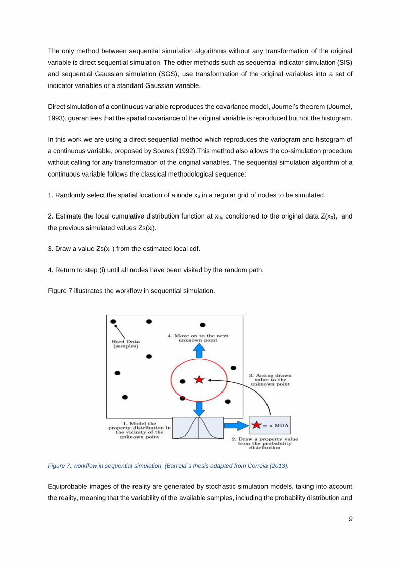
Figure 7 illustrates the workflow in sequential simulation.
Figure 7: workflow in sequential simulation, (Barrela´s thesis adapted from Correia (2013).
Equiprobable images of the reality are generated by stochastic simulation models, taking into account
the reality, meaning that the variability of the available samples, including the probability distribution and

10
the spatial continuity of the samples, revealed by variogram and covariance, should be considered
(Caragea & Smith, 2006).
We are able to characterize the uncertainty of a given phenomenon, by running a large number of
simulations.
2.2.2 Direct-Sequential Simulation
One of the important features of Direct Sequential Simulation is performing simulation without any
transformation in the original variable, so it does not require any prior indicator coding or multi-Gaussian
assumptions. As long as the conditional distributions identify the local kriging means and variances, the
covariance model is reproduced.
Direct sequential simulation has been used for spatial characterization of categorical variables such as
lithotypes, forest species, and soil types (Soares, 1998). Lack of having the equivalent of the normal
score back transform, in the often used sequential Gaussian Simulation (SGS) algorithm, in DSS
algorithm, reproducing histogram becomes an issue.
In 2001, Soares proposed a solution, which is sampling the global target histogram at each simulation
node, by means of simple kriging, so we can identify the local kriging mean and variance. honoring the
covariance model, this method provides an approximation of the target histogram, which results in a re-
sampling of the global cdf FZ(Z) in order to obtain a new distribution FZ'(Z), with its intervals centered on
the local mean and with a spread proportional to the conditional local variance (Soares,2001). This
process will determine the local cdf, at all locations along the path, so at the end of each realization, the
marginal distribution is approximated.
DSS can be summarized by the following algorithm (Soares 2001):
A random path is defined that covers all the nodes to simulate xu, where, u = 1, N and N equals
the number of node to be simulated.
The local mean and variance of Z(xu), is estimated, then respectively the simple kriging is
estimated Z(xu)*, and the estimation variance σ2sk (xu), conditioned to the experimental data Z(xi)
and previous simulated values zS(xi)is calculated.
Interval of the global cdf Fz (z) to be sampled is defined by using the algorithm proposed by
Soares 2001.
From the selected interval of the global cdf Fz (z), a simulated value zS(xu) is drawn.

11
2.2.3 Direct-Sequential Co-Simulation
Direct Sequential Co simulation is an extension of DSS, for spatially dependent variables (Soares,
2001). By using Co-DSS, the individual distributions and the variograms should be reproduced.
Specifically, the generated values must be reproduced based on a joint simulation or co-simulation. As
mentioned before, ability of reproduction of the variograms and covariograms of the simulated variables,
is one of the biggest advantage of Co-DSS comparing with Gaussian Co- simulation (Co-SGS).
Simplicity, efficiency and the possibility of choosing which variable will condition the covariate (primary
variable), is the main advantage of sequential approach. The primary variable is chosen because of its
clear spatial continuity or given its relevance for the case study (Almeida and Journel 1994).
This method that was proposed by Soares, succeeds in reproducing the experimental bivariate and the
conditional distributions.
With two variables of Z1(x), and Z2(x), considering Z1(x) the most important and with more spatial
continuity (Almeida and Journel 1994), the algorithm of joint simulation is described in the following:
1. A random path that encompasses all the nodes of a regular grid is defined.
2. The value z1s (xu), at each node xu , is simulated using DSS algorithm:
The local mean and variance of Z1(x) is estimated, as the SK estimate and estimation
variance z1(xu)* and σ2sk (xu);calculate y(xu)=ᵠ1( z (xu)* ), ᵠ1 being the normal score
transformation of the primary variable Z1(x);
Generate a vale p from a uniform distribution U(0,1);
Generate a value ys from G(y(xu)*,σ2sk (xu)): ys=G-1(y(xu)*, σ2
sk (xu), p);
Return the simulated value z1s (xu) = ᵠ1
-1(ys) of the primary variable.
To simulate z2(x),the same DSS algorithm is applied, while assuming the previously simulated z1(x) as
the secondary variable. In order to calculate z2(xu)* and σ2sk (xu) conditioned to neighbourhood data
z2(𝑥𝛼) and the collocated datum z1(xu) (Goovaerts,1997) , collocated simple cokriging is used.
[𝑧2(𝑥0)]𝑐𝑠𝑘∗ = ∑ 𝜆𝛼[𝑧2(𝑥𝛼) − 𝑚2] + 𝜆𝛽[𝑧1
𝑠𝑁𝛼=1 (𝑥0) − 𝑚1] + 𝑚2 Equation 2
Transform y(xu)* = ᵠ2 z2(xu)*. ᵠ2 which is the normal score transformation of the Z2(x)
variable.
Generate a value p from a uniform distribution U(0,1);
Generate a value ys from G (y2(xu)*, σ2sk (xu): ys = G-1 (y2(xu)*, σ2
sk (xu),p);
Return the simulated value zs (xu) = ᵠ2-1(ys) of the secondary variable.
3. Loop until all nodes are simulated.

12
This methodology also can be extended to the joint simulation of Nv variables.
2.2.4 The use of DSS and Co-DSS as a perturbation method
In this work, we are using the ideas that were proposed by A.Soares, J.D.Diet & L.Guerreiro (2007).
This method is based on two key ideas: the use of the sequential direct co-simulation as the way of
transforming 3D images in an iterative process and to follow the sequential procedure of the genetic
algorithm optimization to converge the transformed images towards an objective function, which will be
discussed.
By using the global and local correlation coefficient, we know how much close is a given generated
images from the objective.
To create the next generation of images, the correlation coefficient of different simulated images are
used as the affinity criterion, until converge to a given predefined threshold is achieved.
Considering set of Ni images, Z1(x), Z2(x),…, , ZNi(x), with the same spatial dispersion statistics,
variogram, and global histogram: , C1(h), , Ɣ1(h), , Fz1(z), we aim to obtain a transformed image , Zt(x).
Direct co-simulation of Zt(x), having Z1(x), Z2(x)… ZNi(x) as auxiliary variables can be applied (Soares,
2001). The collocated cokriging estimator of Zt(x) becomes:
𝑧𝑡(𝑥0) ∗ − 𝑚𝑡(𝑥0) = ∑ 𝜆𝛼(𝑥0)[𝑧𝑡(𝑥𝛼) − 𝑚𝑡(𝑥𝛼)] + ∑ 𝜆𝛼𝑖(𝑥0)[𝑧𝑖(𝑥𝛼) − 𝑚𝑖(𝑥0)]𝑁𝑖𝑖=1
𝛼 Equation 3
Since the models Ɣi(h), i=1 , Ni, and Ɣt(h), are the same, the Markov approximation could be applied.
The affinity of the transformed image Zt(x), with the multiple images Zi(x) are determined by the
correlation coefficients ρt,i(x). So, one can select the images which characteristics we wish to preserve
in the transformed image Zt(x).
2.3 Dynamic Model
After achieving static model, a dynamic model should be used to mimic the production behaviour. The
dynamic model combines the static model and the dynamic properties in order to calculate the
production profiles vs. time, in order to be able to understand and describe the dynamic behaviour of a
hydrocarbon reservoir, thus we can predict its future performance under different development and
production strategies.

13
2.3.1 Constraining the reservoir model
A dynamic reservoir simulation model reflects the version of the partial differential equations that
describes multiphase flow in the subsurface. Equal to partial differential equations, in order to obtain a
solution, furthermore the initial conditions during initialization, we need to set boundary conditions.
The production liquid rate of individual wells is the most common boundary conditions. The choice of
which production data to be used depends on the hydrocarbons present in the reservoir. If the reservoir
produces oil, it is common to use the oil production rate as a conditioning variable, and simply gas ratio
in a gas reservoir. In a case that the oil reservoir produces at high gas-oil ratio (GOR) or high water cut
(WC), it might be better to constrain production by either gas or water production rate ( Ertekin, Abou-
Kassem and king, 2001).
The reason for choosing the constraints depends also on the availability of data, Arpat, G. B. (2005).
For example only recently, pressure sensors are installed downhole to record the pressure continuously,
we can use bottom hole pressure as a constraint as well. Another reason to specify oil rate is to
accurately account for production of the most valuable fluid, oil, in the reservoir (Gilman and Ozgen,
2013).
2.3.2 Matching Criteria
Matching a reservoir model perfectly to historical performance model is a difficult task. Because of that
no standard matching criterias exist which can describe what is considered as an accurately matched
reservoir model (Baker et al., 2006). So we need to establish some sort of criteria which will contain a
successful match. Based on the inherent uncertainty and how much they affect the model performance,
the performance data need different matching criterias.
Another factor could be the production life of the reservoir, because the risk tolerance of most of the
fields tightens as it get more matured, so the matching criteria may change with time (Baker et al.,
2006).For example, matching cumulative oil production to a tighter tolerance than BHP is the general
standard, because oil production is much more important for project economies.
Comparing with the performance data required to match, model performance can be evaluated on a
field level or individual well level. Level of matching to the recorded performance data comparing with
field performance is expected to be higher than individual wells (Mattax and Dalton, 1990).
Set of matching criterias which are listed in Table 1, when we want to determine if the history match is
successful, are proposed by Baker et al. (2006).Taking into account that the trend is followed in addition
to the matching criteria. To wrap it up, we have to realize that a set of matching criterias should be fixed
before history matching, and these criterias are specific for each reservoir. Arranged matching criterias

14
should only be used as guidelines for establishing appropriate basis. This indicates that in the model,
drive mechanism and reservoir physics should be correctly represented, at least to some degree.
Table 1: Matching Criteria used to describe a successful history match (Baker et al., 2006)
Parameter Matching Criteria
Cumulative production (Oil, gas and water) ±10%
Production rate (Oil, gas and water) ±10%
Bottomhole flowing pressure ±20%
Field average pressure ±10%
A history match can be considered as successful when it is following the reservoir performance trend.
Finally if the history matched model is considered successful and meets the matching criteria, then it
could be used for reservoir performance prediction with the same accuracy and uncertainty reflected by
the matching criteria.
2.4 History Matching
2.4.1 Introduction
History matching is a technique to build and interpret the dynamic historical data in a mathematical
model of reservoir from a set of observed data. The model is adjusted and calibrated to match the past
behavior of the reservoir. In other words, history matching is the selection of reservoir models which
best match the reservoir initial data (static and dynamic data).
The following points should be noted during the calibration process:
Mathematical models are based on the observed data. Therefore, any error and approximation
on the data affects the model and its output.
The model is created based on the collected data in the past to predict the future response of a
physical phenomenon and therefore there is an associated error inherited in the process.
Approximation in the model input creates error in the model output.
Error is inevitable in the data observation process.

15
In history matching problems, we know the solution which is the historical production model, but lack of
information about the unknown model parameters (porosity and permeability), makes this algorithm an
ill-posed inverse problem.
In terms of reservoir management, it means that we know the observed dynamic model from the current
producing wells, which helps us planning the future exploration, taking into account the economic
constraints, by reducing the uncertainty associated with the information we have about petrophysical
properties such as porosity and permeability.
Including all the information of dynamic data, and measuring the uncertainty consistently, is a big
challenge in reservoir modelling.
In the process of history matching, we have to update the geological model dynamic data, because they
are an important information source.
History matching can be considered as a continuous improvement method, and a reservoir
characterization validation, because it is a data driven and usually is applied at later stages of reservoir
life. Because the more data we have, the stronger base is for history matching, and these production
information are more available throughout the reservoir production life.
Following steps can be considered for a history matching process (Ertekin, Abou-Kassem and King,
2001):
1. Set the objective function of the history matching process.
2. Delineate the method of the history matching which should be aligned with the objective of the
history matching, and constraints. Constraints can be the project resources, deadlines, data
availability, and etc.
3. Choose or collect the data set and the matching criteria.
4. Those parameters of reservoir that can be adjusted should be determined and also the confidence
range for these parameters should be decided. Those parameters that have the most significant
impact on the reservoir performance.
5. Run the simulation model.
6. Compare the simulation model results with the data in Step 3.
7. Change the model parameters that were defined in Step 4. Note that that change should be within
the physical range of the parameters.
8. Repeat steps 5 through 7 until the criteria set in Step 3 are met.

16
Caers (2002) introduces the combination of history matching with geo statistical modeling with use of
Marcov Chain techniques. In a nutshell, history matching process is initiated with an initial model, then
sets of simulations which are conditioned to the historical production data, are run. Then we have to
compare it with the matching criteria, and if the match is not acceptable, the most uncertain parameters
have to be changed and updated. Parameters that should be changed are those that are causing the
problem.
The model is rerun and compared with the observed data, until a satisfactory match is achieved (Mattax
and Dalton, 1990; Gilman and Ozgen, 2013).
2.4.2 Geostatistical History Matching Workflow
The general reservoir modeling and history matching workflow is described in figure 8 (Streamsim,
2016). Based on this workflow, first we have to build a satisfactory model. Sets of the data source, which
are described in the following, should be integrated, in order to establish a realistic model;
Geological interpretations; which from them (ex., outcrops, cross sections) the environmental
deposition and architectural elements can be deducted.
Well logs; reservoir properties such as porosity, permeability, saturation, stratigraphic top
picks selection can be established.
Cores; Flow characterization for permeability and relative permeability moreover than facies
description are established based on core measurements.
Geochemistry; for establishing a fluid characterization PVT is used.
Seismic; the basis for structural and property analysis are driven from seismic. Reservoir
depletion can be understood from 4D seismic.
Drilling records; Location of the wells in the model are dictated by the surveys from the drilling
operations.
Production profiles; Data about reservoir geometry and flow regimes can be deducted from
production profiles. Estimates of permeability can be analyzed from pressure transient
analysis.
Repeat formation test (RFT); In order to find flow barriers and to know the location of the
reservoir producing parts, saturation and pressure along the wellbore should be measured at
different times.
The starting point for the history matching process will be formed when an acceptable characterized
model is established.
After the initial model is created, simulations will be done and in order to improve the match towards
observed data, perturbations will be performed on different parameters.

17
In geostatistical history matching procedure, this perturbation step is performed with stochastic
simulation and co-simulation in order to maintain the geological consistency and also honoring the wells
and log data.
The convergence speed depends on the reservoir characterization that is done based on the hard data
, logs and reservoir understanding, and the closer description to the real reservoir description, the more
rapid convergence to the historical data match will be achieved, (Gilman and Ozgen,2013). This
highlights the importance of setting a solid understanding of the reservoir.
figure 8: :Schematic diagram of general modelling workflow including the following elements: Parameters,
Sensitivity Runs & Analysis, Screening, and Model Refinement.
In order to be able to do the functional history matching some sort of historical performance data, such
as different phases production rates, pressures, or any other historical data that describes the reservoir
performance, as well as static properties must exist (Ertekin, Abou- Kassem and King, 2001).By
constraining the simulation models to these historical data, we can compare the calculated model
response with any other historical model available.
For instance it could be possible that the simulated model is constrained to well oil rate. So the
corresponding gas and water rates, according to mobility and pressure will be calculated, and can be
compared to the historical reservoir performance.
We need to predetermine criteria which are used to describe a successful match, because there is
always some sort of deviation between the simulation model behaviour and the actual reservoir.

18
Chapter 3
3 Methodology and workflow
The proposed history matching methodology encompasses two different kind of perturbation that will be
discussed deeply in section 3.1, and 3.2.
The first one is Global perturbation which uses a global match (objective function) for all the production
wells, and the second one, local perturbation, which uses different matches for the different production
wells
The proposed methodology is based on the works of Mata-Lima (2008) and Christie et al. (2013) and
can be summarized by the following workflow.
1. Simulation of a set of permeability and porosity realizations through DSS, honouring the well data,
histograms and spatial distribution revealed by the variogram;( the exploratory data analysis of hard
data will be done in section 4.2)
2. Evaluation of the dynamic responses for each of the realizations and calculation of the mismatch
between the dynamic response and real production data, using an objective function;
3. Creation of a composite cube of porosity and permeability, with each region being populated by the
corresponding realization with the least mismatch.
4. Return to step 2, using Co-DSS and the cubes calculated in step 3 and step 4 as, respectively,
correlation data and soft data. The algorithm is expected to run up to a maximum number of iterations
or until a predefined mismatch value is reached.
3.1 Regionalization of the reservoir into different zones
We decided to divide the reservoir into 7 different zones to be more consistent with the spatial continuity
and the petro physical adaptivity, and to maintain the spatial continuity of the reservoir.
Regionalization of the reservoir according to the different layers in depth resulting in a cube with a zone
being assigned for each layer, shale and sand in depth is shown in figure 9.

19
Figure9: Reservoir Zonation in depth consistent with layers
In the process of this thesis we are going to apply two methods of perturbation: global and local.
3.2 Global Perturbation
This is the case where one decides to evaluate the history matching performance with one global
objective function for the entire set of wells.
The global perturbation is a method in which the static properties of reservoir, porosity and permeability,
are perturbed globally. In Co-DSS method (2.2.3), it uses the same correlation coefficient for the entire
field.
A short description of the global method of Mata-Lima (2008) is presented, in order to introduce the
probability perturbation workflow.
In this approach, a porosity image is created using DSS. And after the porosity model is created for a
realization, through a Co-simulation a permeability model is created. In this method just one correlation
coefficient is applied and it is assumed to be global and valid for the entire field. After set of permeability
images are simulated, a secondary image is composed (the best), to be used as secondary information
to generate new realizations by Co-DSS.
The schematic workflow of my project, based on global perturbation is shown in figure 10.

20
Figure. 10: Schematic workflow of the global methodology used in the proposed thesis.
The next section describes local perturbation method which is done by Hoffman & Caers (2005),
Mata-Lima (2008) and Le Ravalec- Dupin & Da Veiga (2011).
3.3 Regional Perturbation
The main problem of using just one match criterion is that the global perturbation can assure the
convergence at the set of wells, but does not assure the convergence of each individual well.
The global method works well for the reservoirs with almost constant geology and are relatively small in
size. But in the reservoirs with larger size that geology is changing too much, and multiple wells exist in
the field, only single match criterion may not be adequate for matching all the data.
Considering the scenario where the reservoir has two production wells in different areas, in the process
of history matching , in a specified iteration , the historical production data of one section may be
matched, while from the other area may not. In the previously described method `global` both sections
of the reservoir are perturbed by similar match criterion, so when trying to match the data in one region,
the match in another region may not be converged.

21
The idea of regional perturbation is basically to allocate an area of influence of each production well,
and to stablish a match criterion for each area of influence, based on the dynamic performance of
producing wells.
Based on the method proposed by Mata-Lima (2008) the geological characteristics of the reservoir,
porosity and permeability, are perturbed locally, using DSS and Co-DSS with multi-distribution functions
and spatial continuity patterns (Nunes, et al., 2016).
After each iteration, best porosity and permeability cube should be created and the perturbation on
properties model should be conditioned to this cube, as a secondary variable ( soft data), through a
correlation coefficient that is calculated based on the dynamic data evaluation , the detailed description
on the calculation of correlation coefficient will be given in section 3.3.2.
The schematic workflow of my project, based on local perturbation is shown in figure 11.
Figure. 11: Schematic workflow of the local perturbation methodology used in the
proposed thesis.
Discussion on region definitions will be done in the following section;
3.3.1 Voronoi zonation
There are some methods to define regions of influence around producer wells. Stream lines technique,
a fast dynamic simulator can be used to define those influence zones (Miliken et al., 2001). In this case

22
the zones are characterized by the dynamic behavior of main perturbation path, the streamlines between
the injector and producer wells. Another alternative is to choose areas of influence based on polygons
which can convey the spatial patterns determined by the variograms.
Since, we need to update the region geometry, based on the modification that is made in the reservoir
model; streamlines could be used successfully in the regionalization methods to define these dynamic
regions. Because they show the exact pathway that fluid enter a production well. These pathways will
have a direct effect on a well´s production. Set of streamlines will enter each production well, and all the
grid blocks are hit by this set of streamlines.
In the process of history matching the facies geometry will change as the model is perturbed. As a result,
the production well´s drainage area will change. In the cases where we have multiple wells in the field
and also the geologic differences in the reservoir, regional perturbations are assimilated. An alternative
static region using streamlines is defined by set of grid blocks that are closest to the production well.
3.3.1.1 Voronoi Polygons
Many GHM algorithms use voronoi polygons to address zonation. Voronoi polygons are an outcome of
a voronoi zonation method whose interior consists of all points in the plane that are closer to a particular
lattice point than to any other, in this case wells, that represents an area of influence of each well.
Figure 12 shows the zonation resulting from the voronoi partition and shows the existence of a zone for
every group of well (zone 1 to 10). Each color represents the area assigned to each production well.
After simulating each realization, a patch of best porosity and permeability is made, along with
composing their respective local correlation coefficient into a cube, which is responsible for strength of
the geostatistical assimilation of properties into next iteration, considering local match quality.
Figure12: Voroni zonation, Region assigned for each well

23
3.3.2 Local Correlation coefficient
During the process of geostatistical history matching, the perturbation which made on all iterations is
carried on the following iterations by means of conditioning, based on the match quality and the
closeness degree to the observed data. This degree of closeness is to the historical production data is
characterized by correlation coefficient applied to every simulated response, which is proposed by
Eduardo Barrela thesis.
A degree of compatibility between the misfit value which is resulted from the objective function and the
correlation coefficient that is used in the co-simulation of a new set of model is ensured in this method.
Also different configurations of obtained simulated values and attempts to keep the calculation of the
resulting correlation coefficients consistent, regarding the relative position between historical and
simulated values as well as their respective error threshold should be taking into account.
The calculation of local correlation coefficient based on Barrela E. (2017) thesis is described in the
following steps:
1. For all the time steps, the deviation from the response toward the observed data and the
error threshold ,Δsim and Δsigma is calculated as the following:
∆𝑠𝑖𝑚 = |𝑅(𝑡,𝑜𝑏𝑠) − 𝑅(𝑡,𝑠𝑖𝑚)| Equation 4
∆𝑠𝑖𝑔𝑚𝑎= 𝜎𝑡2 − ∆𝑠𝑖𝑚 Equation 5
Where Rt,obs is the observed, or historic value of a given variable at timestep t, Rt,sim is the simulated
value of a given variable at timestep t, σ2 is the error, or standard deviation, associated to the
measurement of a given variable at timestep t.
2. Then we have to calculate the final deviation toward observed data, for a given timestep, Δobs.
∆𝑜𝑏𝑠= {𝑅𝑡,𝑜𝑏𝑠 − (∆𝑠𝑖𝑚 + ∆𝑠𝑖𝑔𝑚𝑎) 𝑅𝑡,𝑜𝑏𝑠 ≥ ∆𝑠𝑖𝑚 + ∆𝑠𝑖𝑔𝑚𝑎
0 𝑅𝑡,𝑜𝑏𝑠 < ∆𝑠𝑖𝑚 + ∆𝑠𝑖𝑔𝑚𝑎 Equation 6
3. In order to have a value between⦋ 0, 1⦌, we have to normalize the value of the final
deviation toward observed data, so the correlation coefficient at each time step, xt is
reached.

24
𝑥𝑡 = {1 −
∆𝑠𝑖𝑚
(∆𝑠𝑖𝑚+∆𝑠𝑖𝑔𝑚𝑎+∆𝑜𝑏𝑠)∆𝑠𝑖𝑚≤ ∆𝑠𝑖𝑔𝑚𝑎 + ∆𝑜𝑏𝑠
0 ∆𝑠𝑖𝑚> ∆𝑠𝑖𝑔𝑚𝑎 + ∆𝑜𝑏𝑠
Equation 7
4. The final correlation coefficient is obtained by averaging all the xt from each timestep.
𝑥 =∑ 𝑥𝑡
𝑁𝑡=1
𝑁 Equation 8

25
Chapter 4
4 case study
Productive reservoirs are composed by shallow interbedded sandstone channels and fine shale
laminations with complex geometry.
The quality of available seismic is very poor owing to the fresh water formation which is present in the
reservoir.
The oil productivity in the reservoir is very low, with high water cut, because the paraffinic oil with low
pour point temperature creates conditions for paraffin deposition. Also negligible GOR associated with
the lack of strong aquifer that cause very low initial pressure helps the reservoir pour productivity.
Pilot studies provide an insight into reservoir behavior enabling oil and gas companies to characterize a
reservoir and manage it more effectively.Almost all of the oil accumulated in the basin sandstones was
generated from offshore pods of active source rocks and has migrated laterally for long distances. The
main carrier bed and reservoir of this petroleum system, dips seaward as a regional monocline structure,
with gentle folds, normal faults, and facies changes.
Oil in the main onshore accumulations of the Basin may have been trapped between 1 and 5 m.y. after
the beginning of secondary migration. Significant loss of petroleum may have occurred along seepages
from onshore outcrops of the Formation.
A large carbonate platform, 250 m thick, complete the basin fill. This thickness of carbonate on top of
shallow reservoirs and also the missing of evident structures at reservoir level, induce a very poor
reservoir imaging. Figure 13 shows the position of the reservoir.
Figure 13: Schematic NW-NE section through the basin with red box indicating approximately the position of
reservoir (adapted from Anjos et Al.,2000)

26
4.1 input data
The data that the Company gave us is composed of 12 wells, which two of them are not producing
anymore.
Table2: Wells drilled in the block
Name Well Symbol
P1 OIL
P2 DRY
P3 OIL
P4 OIL
P5 OIL
P6 Planned for water injection
P7 OIL
P8 OIL
P9 OIL
P10 OIL
P11 OIL
P12 OIL
The well locations are shown in Figure 14.

27
Figure 14: Well locations
We had different well logs such as RHOB, GR, PERM, DT, NPHI, PHIE, which are shown in the following
graphic for an example well.
Figure 15: Different well logs shown for Well P1, used as hard data
For hard data, which I used as an input, I upscaled porosity and permeability form the well logs, using
arithmetic mean, showing them in the following.
Figure 16: upscaled porosity from well logs used as hard data
Figure17: upscaled permeability from well logs used as hard data

28
4.1.1 Porosity Permeability relationship
Porosity Permeability relationship clearly shows a positive logarithmic trend in all seven reservoir
levels. Porosity is between 0.001 and 0.3195, and permeability differs from 1.6906 to 5000 md.
Thus, as one of the variable increases the other, behaves the same way. Figure 18 shows the
relation between these two variables in all zones.
The experimental bi histogram is used in the sequential simulation with joint- distribution which
allows the reproduction of the non-linear relationships between properties, in this case porosity
and permeability.
Figure 18: bivariate analysis of Porosity (𝜑) and permeability (K) for different zones.
Horizontal scale (porosity), vertical scale (permeability).
4.2 exploratory data analysis, univariate description and histogram
In the first stage of the project, it is necessary to uni-variate statistical analysis of each of the regional
variables under study, Porosity and Permeability.
With these tools we can draw conclusions about the central tendency and dispersion of the variables, i.e.,
see their variability and trend using the location measurements (mean, median, quartiles and mode) and

29
also see the measures of dispersion (variance, standard deviation and interquartile range).
Table 3 & 4 summarize the property statistics of the hard data, for the variable of porosity and permeability.
Table3: Porosity statistics for different zones
Porosity Zone 0 Zone 1 Zone 2 Zone 3 Zone 4 Zone 5 Zone 6
Mean 0.149151 0.133947 0.111654 0.189173 0.190836 0.129621 0.155807
Std. 0.074091 0.073538 0.094792 0.076770 0.083664 0.07899 0.078070
Minimum 0.001 0.001319 0.001 0.001 0.001073 0.001 0.002239
Maximum 0.311353 0.289549 0.0309721 0.288719 0.306170 0.319500 0.297336
Table4: Permeability statistics for different zones
Permeability Zone 0 Zone 1 Zone 2 Zone 3 Zone 4 Zone 5 Zone 6
Mean 572.4801 786.5778 679.5674 1502.9423 1657.9243 469.0508 1055.9122
Std. 1038.7851 976.2682 1285.8147 1282.1731 1376.3983 1003.2372 1072.4093
Minimum 1.9024 2.09071 1.6906 1.9917 2.0815 1.7671 2.0775
Maximum 5000 3736.6501 5000 4027.3235 4406.0366 5000 3791.8472
The histograms from wells porosity and permeability are presented in the following figures. They represent
the variable distribution and enable the DSS/Co-DSS validation, when compared with the histograms of
the simulated models which are shown in chapter 5.
With histogram, it is possible to proceed to reading the frequencies of occurrences corresponding to each
class;
Figure 19: Porosity (left) and Permeability (right) histogram for zone 0
In the permeability histogram of zone 0, which is shale layer it is easy to distinguish that we have more
population for low permeability’s.

30
Figure 20: Porosity (left) and Permeability (right) histogram for zone 1
In the permeability histogram of zone 1, which is sand layer it is easy to distinguish that we have more
classes of higher permeabilities compared with zone0.
Figure 21: Porosity (left) and Permeability (right) histogram for zone 2
In the permeability histogram of zone 2, which is shale layer it is easy to distinguish that we have again
more population for low permeabilities same as zone0.
Figure 22: Porosity (left) and Permeability (right) histogram for zone 3
In the permeability histogram of zone 3, which is shale layer it is easy to distinguish that we have again
more population for low permeabilities same as zone0.
31
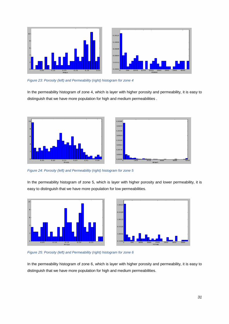
Figure 23: Porosity (left) and Permeability (right) histogram for zone 4
In the permeability histogram of zone 4, which is layer with higher porosity and permeability, it is easy to
distinguish that we have more population for high and medium permeabilities .
Figure 24: Porosity (left) and Permeability (right) histogram for zone 5
In the permeability histogram of zone 5, which is layer with higher porosity and lower permeability, it is
easy to distinguish that we have more population for low permeabilities.
Figure 25: Porosity (left) and Permeability (right) histogram for zone 6
In the permeability histogram of zone 6, which is layer with higher porosity and permeability, it is easy to
distinguish that we have more population for high and medium permeabilities.

32
4.3 direction choice and construction of the variogram
In reservoir simulation we try to describe the spatial distribution of subsurface by integrating all the data
that we have, such as well log data, seismic, geological and production data.
For this set of samples was defined a tolerance of 15 for the permeability and porosity. In this situation,
as the area covered by the acoustic impedance and porosity is less, it means that the set of bins will
depart from the baseline (i.e., the variance) and will describe a behaviour more accurately compared to
a situation which uses a tolerance of 15 to permeability. With this division, it remains to determine the
spatial correlation values to the largest number of possible distances with a reasonable number of pairs
of samples by distance. See appendix A and B for porosity and permeability direction choice based on
variograms and anisotropic direction ellipsoid.

33
Chapter 5
5 Results and Discussion
This section discusses the results obtained by applying the methodology described in Chapter 3, which
was applied to the case study, the Basin introduced in Chapter 4, based on two methods, Global Zonation
and Local zonation.
5.1 Dynamic evaluation
There are two phases in the reservoir: Oil and Water.
The field has 12 wells, 10 producing. The reservoir is controlled by the liquid production rate and the
reservoir will produce during 2770 days.
Based on the initial dynamic data set we were supposed to find a model that gives a good match with
the historical data. The production data that will be used for history matching are Oil production rate and
water production rate.
5.1.1 Objective function
The reservoir has the production in 10 wells during the 2504 days. The conditional data in this case
study is the well log data: Porosity and Permeability; and the production data from each well: water
production rate and oil production rate.
In this workflow, we run 6 iterations, each one with 18 simulations in the global and local perturbation
methods. The misfit depends on the production wells, on the variables: well oil production rate, WOPR,
Well water production rate, WWPR and on the time steps. The objective function applied in this
regionalized geostatistical history matching methodology consist the minimization of the function:
𝑀 = ∑ ∑ 𝑊𝑊𝑃𝑅, 𝑊𝑂𝑃𝑅𝑁𝑣𝑗=1
𝑁𝑤𝑖=1 ∑
(𝑅𝑡,𝑜𝑏𝑠(𝑖,𝑗,𝑡)−𝑅𝑡,𝑠𝑖𝑚(𝑖,𝑗,𝑡))2
𝜎
𝑁𝑡𝑡=0 Equation 9
Where Nw is number of wells, Nv is number of variables, and Nt is number of timesteps.
In history matching technique, the simulated data for each variable is compared to the historical data by

34
means of a misfit function, objective function. Thus, the history matching problem is translated into an
optimization problem in which the misfit function is an objective function bounded by the model
constraints. The objective function is minimized using appropriate optimization algorithm and thus the
results are the model parameters that best approximate the fluid rates and pressure data recorded
during the reservoir life.
Defining objective function is critical, because convergence is achieved through this parameter.
It is defined in most of the history matching problems, as a measure of difference between the simulated
production values and the historical field production data. From objective function, a value of mismatch,
M, is returned, which is the least square norm formulated in this thesis as;
𝑀 = 𝑚𝑖𝑛 ∑(𝑅𝑡,𝑜𝑏𝑠−𝑅𝑡,𝑠𝑖𝑚)
2
𝜎
𝑛𝑡=𝑖 Equation 10
Where Rt,obs stands for the historical production data of a given variable at timestep t, Rt,sim stands
for simulated value of the given variable at timestep t, σ2 is the error, or standard deviation, associated
to the measurement of a given variable at timestep t.
Local correlation coefficient is also accompanied by the described misfit, which is responsible for
conveying the optimal petrophysical parameters information into the next iteration, through geostatistical
assimilation by co-simulation.
5.2 Global zonation
For the global perturbation method we run the model with 6 iterations and 18 simulations, using the
correlation coefficient of 0.8 for all the wells. The minimum misfit happens in iteration 5, simulation 18.
Figure 26 and 28 illustrate the best–fit models (iteration 5, simulation 18) of porosity and permeability
obtained from the application of the GHM algorithm with Global zonation.

35
Figure 26: Best fit Porosity model obtained from DSS, global zonation (Iteration 5, simulation18)
Figure 27: Porosity histogram comparison; well logs (blue), best model from global zonation (green)
%

36
Figure 28: Best fit Permeability model obtained from CO-DSS, global zonation (Iteration 5, simulation18)
Figure 29: Permeability histogram comparison; well logs (blue), best model from global zonation (green)
The general pattern for the run can be characterized by a considerable drop in the results from iteration
1 to iteration 2. After this drop an increase of the values is observed until forth iteration, and then a sharp
drop to iteration 5 and at the last iteration a small increase. This can be explained simply by looking at
the standard deviation per iteration plot (figure 30). Such a quick drop in standard deviation values can
be explained by the type of correlation coefficient used for the global zonation method, which is a global
correlation coefficient of 0.8. Convergence of the run is obtained at iteration 5 with a global minimum
misfit of 5689.06 for the run.

37
Figure 30: Minimum misfit and standard deviation per iteration for global perturbation
5.3 Voronoi zonation
For voronoi zonation we run 18 simulation and 6 iterations. The correlation coefficient that was used on
each realization was calculated based on section 3.2.2. The minimum misfit happens in iteration 5,
simulation 16.
Figure 32 and 34 shows the best–fit models (iteration 5, simulation 16) of porosity and permeability
obtained from the GHM algorithm with Voronoi zonation.
0
1000
2000
3000
4000
5000
6000
7000
IT1 IT2 IT3 IT4 IT5 IT6

38
Figure 31: Zonation polygons used in voronoi simulation
Figure 32: Best fit Porosity model obtained from DSS, Voroni zonation (Iteration 5, simulation16)

39
Figure 33: Porosity histogram comparison; well logs (blue), best model from voronoi zonation (green)
Figure 34: Best fit Permeability model obtained from CO-DSS, voronoi zonation (Iteration 5, simulation16)
%

40
Figure 35: Permeability histogram comparison; well logs (left), best model from voronoi zonation (right)
The general pattern for the run can be characterized by a considerable drop in the results from iteration
1 to iteration 2. After this drop an increase of the values is observed until third iteration, and then a sharp
drop till iteration 5 and at the last iteration a small increase. This can be explained simply by looking at
the standard deviation per iteration plot (figure 36). The correlation coefficient was changed at each time
step based on the calculation that was shown in section 3.3.2. The minimum misfit for the local zonation
was 4793.635, and a drop from 5689.06 to 4793.635 can be seen from the global perturbation method.
Figure 36: Minimum misfit and standard deviation per iteration for local perturbation
Comparison for the static properties (φ, k) from first realization through the last realization is shown in
Figure 37 and 38.
As it is visible in the figures, the original geological trends are kept from the first realization trough the
0
1000
2000
3000
4000
5000
6000
7000
8000
IT1 IT2 IT3 IT4 IT5 IT6
Iteration5,
Simulation
16

41
last one. The comparison of the other zones in top layer, are depicted in Appendix C.
Figure 37: Porosity simulated model for first iteration, first Simulation (above Figure), Porosity global simulated
model for iteration 6, simulation18 (last realization)( bottom left figure), Porosity local simulated model for iteration
6, simulation18 (last realization)( bottom right figure).

42
Figure 38: Permeability simulated model for first iteration, first Simulation (above Figure), Permeability global
simulated model for iteration 6, simulation18 (last realization)( bottom left figure), Permeability local simulated model
for iteration 6, simulation18 (last realization)( bottom right figure).

43
5.4 Production match analysis
In order to do the history matching we run 6 iterations and 18 simulations. For global approach we used
correlation coefficient of 0.8 for all realizations, but in the local approach we used a different correlation
using a different sigma at each timestep based on the observed value for the conditional data. The
methodology was implemented until day 2770.
The production data from the simulated reservoir models match considerably well the production data
from the historical model.
Figure 39 shows the comparison of results between the different adopted zonation methods.
Figure 39: comparison between different zonation methods, global minimum misfit per iteration (red), local
minimum misfit per iteration (blue).
Results in terms of well production rates for all wells are shown in the following figures.
For almost all the wells we have a better match than the geological unmatched model. Depending on
the quantity of the data we had at the timesteps, the match to the observed model was much better
where we had more production data.
The simulated responses for well P1 on water (Fig.40.left) and Oil (Fig.40.right) closely match the
observed production data, on both global and local regionalization methods.
The minimum misfit for global perturbation occurs in iteration 5, simulation 18(Fig.40.up), while for local
perturbation it occurs in iteration 5, simulation 16(Fig.40.bottom).
The dynamic simulated model for well P1 starts from day zero and continues producing until day 2770,
and in day 386 and 1401 it shuts down. And also the trend is almost the same for all the timesteps, but
the local simulated model is much closer to the historical model.
0
1000
2000
3000
4000
5000
6000
7000
8000
IT1 IT2 IT3 IT4 IT5 IT6
min
imu
m m
isfi
t
number of iteration

44
Figure 40:water & oil production simulated model vs history vs geological unmatched model for well P1,global water
production rate(up-left), global oil production rate(up-right), local water production rate(down-left), local oil
production rate(down-right), geological unmatched model (blue), minimum misfit (red), observed model(green).
The simulated responses for well P3 on water (Fig.41.left) and Oil (Fig.41.right) closely match the
observed production data, in local regionalization method, while in the global method the response for
water production is a bit far from the historical data.
The minimum misfit for global perturbation occurs in iteration 5, simulation 18(Fig.41.up), while for local
perturbation it occurs in iteration 5, simulation 16(Fig.41.bottom).
Based on Figure 41, for water and oil production rate, the dynamic simulated model starts from zero day
891 and increases producing until day 2770, the simulated model trend is almost the same for all the
timesteps, but the local simulated model is much closer to the historical model. The OPR simulated
model almost matches the historical model in the local approach.
0
10
20
30
40
50
60
0
21
4
45
7
70
0
89
1
10
95
13
40
14
92
17
37
19
79
22
22
24
67
26
88
WW
PR
(Sm
3/D
AY
),w
ell P
1
Timesteps(days)
0
10
20
30
40
0
21
4
45
7
70
0
89
1
10
95
13
40
14
92
17
37
19
79
22
22
24
67
26
88
WO
PR
(Sm
3/D
AY
), w
ell P
1
Timesteps(days)
0
10
20
30
40
50
60
0
21
4
45
7
70
0
89
1
10
95
13
40
14
92
17
37
19
79
22
22
24
67
26
88
WW
PR
(Sm
3/D
AY
), w
ell
P1
Timesteps(days)
0
10
20
30
40
0
21
4
45
7
70
0
89
1
10
95
13
40
14
92
17
37
19
79
22
22
24
67
26
88
WO
PR
(Sm
3/D
AY
), w
ell
P1
Timesteps(days)

45
Figure 41: water & oil production simulated model vs history vs geological unmatched model for well P3,global
water production rate(up-left), global oil production rate(up-right), local water production rate(down-left), local oil
production rate(down-right), geological unmatched model (blue), minimum misfit (red), observed model(green).
The simulated responses for well P4 on water (Fig.42.left) and Oil (Fig.42.right) closely match the
observed production data, in local regionalization method, while in the global method the response for
water production is a bit far from the historical data.
Based on Figure 42, for water and oil production rate, the dynamic simulated model starts from zero,
day 1028 and continues producing until day 2770, and in day 1401 and 1415 and 2694 it shut down.
The global simulated model is very far from the historical model, but the local approach shows a good
results in terms of similarity in WOPR and WWPR.
0
10
20
30
40
0
21
4
45
7
70
0
89
1
10
95
13
40
14
92
17
37
19
79
22
22
24
67
26
88
WW
PR
(Sm
3/D
AY
), w
ell P
3
Timesteps(days)
0
10
20
30
40
0
21
4
45
7
70
0
89
1
10
95
13
40
14
92
17
37
19
79
22
22
24
67
26
88
WO
PR
(Sm
3/D
AY
), w
ell P
3
Timesteps(days)
0
10
20
30
40
0
24
5
51
8
79
1
10
06
12
48
14
31
17
06
19
79
22
52
25
26
27
00
WW
PR
(Sm
3/D
AY
), w
ell
P3
Timesteps(days)
0
10
20
30
40
0
21
4
45
7
70
0
89
1
10
95
13
40
14
92
17
37
19
79
22
22
24
67
26
88
WO
PR
(Sm
3/D
AY
), w
ell P
3
Timesteps(days)

46
Figure 42: water & oil production simulated model vs history vs geological unmatched model for well P4,global
water production rate(up-left), global oil production rate(up-right), local water production rate(down-left), local oil
production rate(down-right), geological unmatched model (blue), minimum misfit (red), observed model(green).
Based on Figure 43, for water and oil production rate in well P5, the dynamic simulated model starts
from zero, day 1350 and continues producing until day 2770, and in day 1401 and 1415 and 2700 it shut
down. Both global and local simulated models are very similar to historical model for WWPR and WOPR.
0
5
10
15
20
25
30
35
0
24
5
51
8
79
1
10
06
12
48
14
31
17
06
19
79
22
52
25
26
27
00
WW
PR
(Sm
3/D
AY
), w
ell
P4
Timesteps(days)
0
5
10
15
20
0
21
4
45
7
70
0
89
1
10
95
13
40
14
92
17
37
19
79
22
22
24
67
26
88
WO
PR
(Sm
3/D
AY
), w
ell P
4
Timesteps(days)
0
5
10
15
20
25
30
35
0
24
5
51
8
79
1
10
06
12
48
14
31
17
06
19
79
22
52
25
26
27
00
WW
PR
(Sm
3/D
AY
), w
ell
P4
Timesteps(days)
0
5
10
15
20
0
21
4
45
7
70
0
89
1
10
95
13
40
14
92
17
37
19
79
22
22
24
67
26
88
WO
PR
(Sm
3/D
AY
), w
ell P
4
Timesteps(days)
0
5
10
15
20
25
30
0
24
5
51
8
79
1
10
06
12
48
14
31
17
06
19
79
22
52
25
26
27
00
WW
PR
(Sm
3/D
AY
), w
ell P
5
Timesteps(days)
0
2
4
6
8
10
12
0
21
4
45
7
70
0
89
1
10
95
13
40
14
92
17
37
19
79
22
22
24
67
26
88
WO
PR
(Sm
3/D
AY
), w
ell P
5
Timesteps(days)

47
Figure 43: water & oil production simulated model vs history vs geological unmatched model for well P5,global
water production rate(up-left), global oil production rate(up-right), local water production rate(down-left), local oil
production rate(down-right), geological unmatched model (blue), minimum misfit (red), observed model(green).
Based on Figure 44, for water and oil production for well P7, the dynamic simulated model starts from
zero, day 2010 and continues producing until day 2770.The global simulated model is a bit far from
reality, but trying the local simulation resulted in a good match toward historical model in both WWPR
and WOPR.
Figure 44: water & oil production simulated model vs history vs geological unmatched model for well P7,global
water production rate(up-left), global oil production rate(up-right), local water production rate(down-left), local oil
production rate(down-right), geological unmatched model (blue), minimum misfit (red), observed model(green).
Based on Figure 45, for water and oil production for well P8, the dynamic simulated model starts from
0
5
10
15
20
25
30
0
24
5
51
8
79
1
10
06
12
48
14
31
17
06
19
79
22
52
25
26
27
00
WW
PR
(Sm
3/D
AY
), w
ell P
5
Timesteps(days)
0
2
4
6
8
10
12
0
21
4
45
7
70
0
89
1
10
95
13
40
14
92
17
37
19
79
22
22
24
67
26
88
WO
PR
(Sm
3/D
AY
), w
ell P
5
Timesteps(days)
0
5
10
15
20
0
27
6
57
9
85
3
10
95
13
71
16
14
19
18
22
22
25
26
27
09
WW
PR
(Sm
3/D
AY
), w
ell
P7
Timesteps(days)
0
2
4
6
8
10
12
0
27
6
57
9
85
3
10
95
13
71
16
14
19
18
22
22
25
26
27
09
WO
PR
(Sm
3/D
AY
), w
ell
P7
Timesteps(days)
0
5
10
15
20
0
30
4
64
1
91
4
12
18
14
61
17
96
21
30
24
67
27
00
WW
PR
(Sm
3/D
AY
), w
ell
P7
Timesteps(days)
0
2
4
6
8
10
12
0
24
5
51
8
79
1
10
06
12
48
14
31
17
06
19
79
22
52
25
26
27
00
WO
PR
(Sm
3/D
AY
), w
ell P
7
Timesteps(days)

48
zero, day 2375 and continues producing until day 2770.The global simulated model is a bit far from
reality, but the local simulation resulted in a better, but not good match toward historical model in both
WWPR and WOPR, because lack of data.
Figure 45: water & oil production simulated model vs history vs geological unmatched model for well P8,global
water production rate(up-left), global oil production rate(up-right), local water production rate(down-left), local oil
production rate(down-right), geological unmatched model (blue), minimum misfit (red), observed model(green).
Based on Figure 46, for water and oil production in well P9, the dynamic simulated model starts from
zero, day 2375 and continues producing until day 2770 similar to well P8.The global simulated model is
a bit far from reality, but the local simulation resulted in a better, but not good match toward historical
model in both WWPR and WOPR.
0
0.5
1
1.5
2
2.5
3
3.5
0
24
5
51
8
79
1
10
06
12
48
14
31
17
06
19
79
22
52
25
26
27
00
WW
PR
(Sm
3/D
AY
), w
ell P
8
Timesteps(days)
0
1
2
3
4
5
0
21
4
45
7
70
0
89
1
10
95
13
40
14
92
17
37
19
79
22
22
24
67
26
88
WO
PR
(Sm
3/D
AY
), w
ell P
8
Timesteps(days)
0
0.5
1
1.5
0
27
6
57
9
85
3
10
95
13
71
16
14
19
18
22
22
25
26
27
09
WW
PR
(Sm
3/D
AY
), w
ell
P8
Timesteps(days)
0
1
2
3
4
5
0
24
5
51
8
79
1
10
06
12
48
14
31
17
06
19
79
22
52
25
26
27
00
WO
PR
(Sm
3/D
AY
), w
ell
P8
Timesteps(days)
0
0.5
1
1.5
2
0
24
5
51
8
79
1
10
06
12
48
14
31
17
06
19
79
22
52
25
26
27
00
WW
PR
(Sm
3/D
AY
),
wel
lP9
Timesteps(days)
00.5
11.5
22.5
3
0
24
5
51
8
79
1
10
06
12
48
14
31
17
06
19
79
22
52
25
26
27
00
WO
PR
(Sm
3/D
AY
), w
ell
P9
Timesteps(days)

49
Figure 46: water & oil production simulated model vs history vs geological unmatched model for well P9,global
water production rate(up-left), global oil production rate(up-right), local water production rate(down-left), local oil
production rate(down-right), geological unmatched model (blue), minimum misfit (red), observed model(green).
Based on Figure 47, for water and oil production in well P10, the dynamic simulated model starts from
zero, day 2375 and continues producing until day 2770 similar to well P8 & P9.The global simulated
model is a bit far from reality, but the local simulation resulted in a better, but not good match toward
historical model in both WWPR and WOPR, because lack of production data.
Figure 47: water & oil production simulated model vs history vs geological unmatched model for well P10,global
water production rate(up-left), global oil production rate(up-right), local water production rate(down-left), local oil
production rate(down-right), geological unmatched model (blue), minimum misfit (red), observed model(green).
For water and oil production for wells P11 and P12, since these wells only have production in the last
timestep, they are not used in the history matching and zonation discussion.
0
0.5
1
1.5
2
0
24
5
51
8
79
1
10
06
12
48
14
31
17
06
19
79
22
52
25
26
27
00
WW
PR
(Sm
3/D
AY
), w
ell
P9
Timesteps(days)
0
0.5
1
1.5
2
2.5
3
0
27
6
57
9
85
3
10
95
13
71
16
14
19
18
22
22
25
26
27
09
WO
PR
(Sm
3/D
AY
), w
ell
P9
Timesteps(days)
0
5
10
15
0
27
6
57
9
85
3
10
95
13
71
16
14
19
18
22
22
25
26
27
09
WW
PR
(Sm
3/D
AY
),
wel
l P1
0
Timesteps(days)
0
5
10
15
20
0
24
5
51
8
79
1
10
06
12
48
14
31
17
06
19
79
22
52
25
26
27
00
WO
PR
(Sm
3/D
AY
),
wel
l P1
0
Timesteps(days)
02468
10
0
27
6
57
9
85
3
10
95
13
71
16
14
19
18
22
22
25
26
27
09
WW
PR
(Sm
3/D
AY
),
wel
l P1
0
Timesteps(days)
0
5
10
15
20
0
24
5
51
8
79
1
10
06
12
48
14
31
17
06
19
79
22
52
25
26
27
00
WO
PR
(Sm
3/D
AY
),
wel
l P1
0
Timesteps(days)

50
Chapter 6
6 Conclusions and Future work
The motivation behind this work was to understand the real case reservoir, in order to find a proper
model for history matching, so based on this model the decision making regarding the development of
the field, predicting future production, placing additional wells, and evaluating alternative reservoir
management scenarios is possible.
Usually history matching is done on synthetic cases, so doing it for a real case study with complex
stratigraphy was a challenging project, which was done in this thesis. Also history matching, most of the
time, is the process of integrating production data with other source of data such as core samples,
geologic intuition, seismic and well tests, that in our case lack of good seismic due to fresh water
formation, in the other hand, the poor reliability of the data for bottom hole pressures of the wells, lead
to use the WOPR and WWPR for conditioning the wells in production simulations, because, after
analysing the data, we understood the importing data for BHP was not reliable, due to inaccuracy of
sampling downloading data. All these together, made history matching more complicated.
A work flow based on the partitioning the reservoir into different zones, presenting very promising
results, although the method shows a fast convergence, since this method only uses the production
history and static data as a conditioning data, it would be more convenient if we had a seismic inversion
to integrate it with parameter perturbation.
The successful application of the proposed methodology for a real case studies delivers good
perspectives for its application to other real case studies with different geologies and geometries.
Further studies on this area could be focused towards prediction of reservoir behaviour with a degree
of uncertainty and also towards other types of parameter perturbation or towards its integration with
seismic inversion.
For the basin under study, in specific, research on how the oil production rate could be increased, by
planning injection wells, for pressure support, could be done.

51

52
Refrences
Arpat, G. B. (2005), Sequential simulation with patterns, Stanford University.
Baker et al, (2006), History Matching Standards; Quality Control and Risk analysis for Simulation. Paper
2006-129 (Canadian International Petroleum Conference).
Barrela, E. J. A. (2016), Geostatistical History Matching coupled with Adaptive Stochastic Sampling,A
zonation-based approach using Direct Sequential Simulation.
Bertolini, A. & Schiozer, D. (July 2011) Influence of the objective function in the history matching
process, Journal of Petroleum Science and Engineering.
Caers, J. (2002), History matching under geological control with the probability perturbation method, Department of Petroleum Engineering Stanford University.
Caragea, P. and Smith, R. (2006), approximate likelihoods for spatial processes,Preprint.
Correia, P. (2013, March). Student Garden Geostatistics course. Retrieved from ResearchGate:
https://www.researchgate.net/publication/268811925_Student_Garden_Geostatistics_course
Dean C. Rietz, Miles R. Palke. (2001), History matching helps validate reservoir simulation models, Oil &Gas Jounal, Washington pulse.
Deutsch, C.V. and Journel, A.G. (1998). GSLIB Geostatistical Software Library and User's Guide, 2nd Edition, Applied Geostatistics Series, Oxford University Press, Inc. New York, NY.
Ertekin, T. & Abou-Kassem, J. H. and King, G. R. (2001), Basic Applied Reservoir Simulation, Society
of Petroleum Engineering.
Goovaerts, P., (1997). Geostatistics for Natural Resources Evaluation. Oxford University Press, New York, 483p.
Hernandez, G., Journel, A.G. (1994), Stochastic Characterization of Gridblock Permeabilities, SPE
Formation Evaluation, 9 (2) pp. 93-99 CrossRefView Record in Scopus.
Hoffman, B. T. & Caers, J. (2005), Regional probability perturbations for history matching, Stanford
University.
Hohn, M. E. (1999). Geostatistics and Petroleum Geology. Kluwer Adademic Publishers.
Horta, A., Soares, A. (2010), Direct Sequential Co-simulation with Joint Probability Distributions,
nternational Association for Mathematical Geosciences.
James R., Gilman and Ozgen, C. (2013), Reservoir simulation: history matching and forecasting, Society
of Petroleum Engineers.
Journel AG, Huijbregts CJ (1978) Mining geostatistics. Academic, New York, p 600, Google Scholar
Journel, A.G. (1993) Geostatistics: Roadblocks and Challenges, In Soares, A (ed.) Geostatistic–Troia,
Kluwer, Dordrecht, 213-244.

53
Le Ravalec-Dupin, M. & Enchery, G. & Baroni, A. and Da Veiga, S. (2011), Preselection of Reservoir
Models From a Geostatistics-Based Petrophysical Seismic Inversion, IFP Energies Nouvelles.
Mata-lima, H.; Vargas, H.; Carvalho, J.; Goncalves, M.; Caetano, H.;Marques, A.; Raminhos, C.
Comportamento hidrológico de bacias hidrográficas:integração de métodos e aplicação a um estudo de
caso. Revista Escola de Minas, v. 60, n. 3, 2007.
Mata-Lima, H. (2008), Reservoir characterization with iterative direct sequential co-simulation:
Integrating fluid dynamic data into stochastic model, Journal of Petroleum Science and Engineering.
Maraschin, A., Mizusaki, A. & De Ros, L. (2004), Near-Surface K-Feldspar Precipitation, Northeastern
Brazil, Instituto de Geocieˆ ncias, Universidade Federal do Rio Grande do Sul.
Marco A.S. Moraes and Ronald C. Surdam, (1993), Digenetic heterogeneity and reservoir quality; Flovial
Deltaic and Turbiditic Sandstone Reservoirs, the American Association of Petroleum Geologists Bulletin.
Marques, C. R. F. (2015), Multiscale Geostatistical History Matching Using Block Direct Sequential
Simulation and Uncertainty Quantification, IST.
Mattax, C. C. & Dalton, R. L. (1990), Reservoir Simulation, Society of Petroleum Engineers.
Milliken et al.,W.J. Milliken, A.S. Emanuel, (2001), A. Chakravarty Applications of 3D streamline
simulation to assist history matching, SPE J. RE and E pp. 502-508.
Nunes, R., Soares, A., Azevedo, L., & Pereira, P. (2016). Geostatistical Seismic Inversion with Direct
Sequential Simulation and Co-simulation with Multi-local Distribution Functions. Mathematical
Geosciences, 1-19.
Pettersen, (2006) Basics of Reservoir Simulation with the Eclipse Reservoir Simulator, Dept. of
Mathematics, University of Berge.
Petruta, C. & Caragea, P. C. and Smith, R. L. ( 2006) Asymptotic properties of computationally efficient
alternative estimators for a class of multivariate normal models, Department of Statistics, Iowa State
University.
Pereira Carneiro, J. D. T. (2010), Multi-Objective Stochastic Optimization by Co-Direct Sequential
Simulation for History Matching of Oil Reservoirs, Dep. Mines, IST, Lisbon, Portugal.
Press et al. & Press, W.H. & Teukolsky, S.A. & Vetterling, W.T. and Flannery, B.P. (1989), Numerical
Recipes in Fortran, Cambridge University Press.
Shams, M. (2016), Reservoir Simulation Assisted History Matching: From Theory to Design, (Amal Petroleum Company) SPE Kingdom of Saudi Arabia Annual Technical Symposium and Exhibition, 25-28 April, Dammam, Saudi Arabia.
Soares, A., (1998), Sequential indicator simulation with correction for local probabilities: Math. Geology, v. 30, no. 6, p. 761–765.Google Scholar
Soares, A. (2001), Direct Sequential Simulation and Cosimulation, Mathematical Geology.
Soares, A, J.D.Diet & L.Guerreiro. (2007), Stochastic Inversion with a Global Perturbation Method,
Petroleum Geostatistics, Cascais, Portugal.
Streamsim,(2016),retrieved from,
http://www.streamsim.com/sites/default/files/genmodelingworkflow.png.

54
Trindade, L. A. F & Brassel, S. C. and Santos Neto, E. V. (1992), Petroleum Migration, the American
Association of Petroleum Geologists Bulletin.

A
Appendix A – Porosity Direction Choice
Figure 1: Porosity variogram (3 figures on the left), anisotropic direction ellipsoid which was used for direction
choice (right figure) for zone 0
Figure 2: Porosity variogram (3 figures on the left), anisotropic direction ellipsoid which was used for direction
choice (right figure) for zone1
Figure 3: Porosity variogram (3 figures on the left), anisotropic direction ellipsoid which was used for direction
choice (right figure) for zone2
Figure 4: Porosity variogram (3 figures on the left), anisotropic direction ellipsoid which was used for direction
choice (right figure) for zone3

B
Figure 5: Porosity variogram (3 figures on the left), anisotropic direction ellipsoid which was used for direction
choice (right figure) for zone4
Figure 6: Porosity variogram (3 figures on the left), anisotropic direction ellipsoid which was used for direction
choice (right figure) for zone5
Figure 7: Porosity variogram (3 figures on the left), anisotropic direction ellipsoid which was used for direction
choice (right figure) for zone6

C
Appendix B – Permeability Direction Choice
Figure 1: Permeability variogram (3 figures on the left), anisotropic direction ellipsoid which was used for direction
choice (right) for zone0
Figure 2: Permeability variogram (3 figures on the left), anisotropic direction ellipsoid which was used for direction
choice (right) for zone1
Figure 3: Permeability variogram (3 figures on the right), anisotropic direction ellipsoid which was used for
direction choice (right) for zone2
Figure 4: Permeability variogram (3 figures on the left), anisotropic direction ellipsoid which was used for direction
choice (right) for zone3

D
Figure 5: Permeability variogram (3 figures on the left), anisotropic direction ellipsoid which was used for direction
choice (right) for zone4
Figure 6: Permeability variogram (3 figures on the left), anisotropic direction ellipsoid which was used for direction
choice (right) for zone5
Figure 7: Permeability variogram (3 figures on the left), anisotropic direction ellipsoid which was used for direction
choice (right) for zone6

E
Appendix C – Static Porosity Models for different zones
Comparison of the static Properties, Porosity and Permeability from first realization through the last
realization for different zones, all in top layers, are shown in the following figures. The top layer that was
shown in section 5.3 is for zone 7 (top layer).
Looking at all the images, it can be seen that in all layers, the original geological features are kept from
the first realization trough the last one.
Figure 1: Porosity Simulated model for first iteration, first Simulation (left Figure), global (Middle figure), local (right
figure), top layer of zone 6.
Figure 2: Permeability Simulated model for first iteration, first Simulation (left Figure), global (Middle figure), local
(right figure), top layer of zone 6.

F
Figure 3: Porosity Simulated model for first iteration, first Simulation (left Figure), global (Middle figure), and local
(right figure), top layer of zone 5.
Figure 4: Permeability Simulated model for first iteration, first Simulation (left Figure), global (Middle figure), local
(right figure), top layer of zone 5.
Figure 5: Porosity Simulated model for first iteration, first Simulation (left Figure), global (Middle figure), and local
(right figure), top layer of zone 4.

G
Figure 6: Permeability Simulated model for first iteration, first Simulation (left Figure), global (Middle figure), local
(right figure), top layer of zone 4.
Figure 7: Porosity Simulated model for first iteration, first Simulation (left Figure), global (Middle figure), and local
(right figure), top layer of zone 3
Figure 8: Permeability Simulated model for first iteration, first Simulation (left Figure), global (Middle figure), local

H
(right figure), top layer of zone 3
Figure 9: Porosity Simulated model for first iteration, first Simulation (left Figure), global (Middle figure), and local
(right figure), top layer of zone 2.
Figure 10: Permeability Simulated model for first iteration, first Simulation (left Figure), global (Middle figure), local
(right figure), top layer of zone 2.
Figure 11: Porosity Simulated model for first iteration, first Simulation (left Figure), global (Middle figure), and local
(right figure), top layer of zone 1.

I
Figure 12: Permeability Simulated model for first iteration, first Simulation (left Figure), global (Middle figure), local
(right figure), top layer of zone 1.
Figure 13: Porosity Simulated model for first iteration, first Simulation (left Figure), global (Middle figure), and local
(right figure), top layer of zone 0.
Figure 14: Permeability Simulated model for first iteration, first Simulation (left Figure), global (Middle figure), local
(right figure), top layer of zone 0.