Multivariate Lorenz dominance based on zonoids

Multivariate Lorenz dominance based on zonoids∗

Gleb A. Koshevoy and Karl Mosler

November 17, 2006

Abstract

The classical Lorenz curve visualizes and measures the disparityof items which are characterized by a single variable: The more thecurve bends, the more scatter the data. Recently a general approachhas been proposed and investigated that measures the disparity ofmultidimensioned items regardless of their dimension.

This paper surveys various generalizations of Lorenz curve andLorenz dominance for multidimensional data. Firstly, the Lorenzzonoid of multivariate data and, more general, of a random vectoris introduced. Then three multivariate extensions of univariate Lorenzdominance are surveyed and contrasted, the set inclusion of lift zonoids,the scaled convex order, and the price Lorenz order. The latter is basedon the set inclusion of extended Lorenz zonoids. Finally, a decomposi-tion of the multivariate volume-Gini mean difference is given.

Keywords: Multivariate Lorenz order, directional majorization, price Lorenzorder, generalized Lorenz function, multidimensioned Gini index.

AMS (2000) Subject Classification: Primary 60E15, Secondary 62H99,91B14.

JEL: C49, D31, D69, I30.∗Paper presented to the ‘International Conference in Memory of Two Eminent Social

Scientists: C. Gini and M.O. Lorenz’, Siena 2005. We thank Achille Lemmi and manyparticipants for discussions as well as the Editor and an unknown referee for their valuableremarks.

1

1 Introduction

Max O. Lorenz [27] has introduced a special tool to visualize data. He rep-resented the distribution of relative data (that is, data over their mean) bya curve, his celebrated Lorenz curve. We stress three of Lorenz’ achieve-ments: (1) The Lorenz curve is visual: it indicates the degree of disparity‘the more the curve is bent’. (2) Up to a scale parameter, the Lorenz curvefully describes the underlying distribution. (3) The pointwise ordering ofLorenz curves provides an ordering of disparity, the Lorenz dominance.

Originally designed to visualize data on household incomes and compareeconomic inequality, the Lorenz curve has been employed in virtually everyfield of statistical application. In the economic and social sciences Lorenzdominance has been used to measure economic inequality and poverty [11,2, 37], industrial concentration [9], social segregation [1], the distribution ofpublishing activities [8], ecological diversity [31], and many others. The Giniindex, which is twice the area between the Lorenz curve and the diagonal ofthe unit square, serves as the most popular index of income inequality. Acomprehensive guide to the widely dispersed literature on Lorenz dominanceup to 1993 is provided by [28]; for more recent applications, see [35].

Generally, the Lorenz curve measures sort of scatter or dispersion with re-spect to a single variable. In many of these applications it is natural toconsider several variables instead of a single one and to measure their dis-persion in a multivariate setting. E.g., economic inequality with respect toincome and wealth, poverty in terms of income, education and health.

In comparing two distributions of multiattribute endowments, we may checkeach of the attributes separately. However, looking only at the marginaldistributions neglects possible dependencies in the value of attributes. E.g.,income may be substituted by wealth. In such a case, joint distributionshave to be investigated and compared.

Multivariate comparisons are either based on real-valued indexes, whichyield complete orderings of distributions, or on partial orderings. The usualLorenz dominance is a partial ordering in dimension one. Special indexes ofmultivariate economic inequality have been proposed by [26, 39], and others.Also, partial orderings of multivariate inequality have been introduced byvarious authors, among them [12, 3, 4, 30]. Kolm [12] orders distributions

2

of multivariate endowments by matrix majorization, which amounts to theconvex scaled order mentioned below; in dimension one, it is the usual Lorenzdominance.

This paper surveys several extensions of Lorenz dominance and Lorenz curveto multidimensional data. Each of the multivariate ordering relations dis-cussed in the sequel implies Lorenz dominance of the marginals. From givendata, marginal Lorenz dominance can be checked by inspection of the Lorenzcurves; this provides a simple necessary condition for multivariate domi-nance. A sufficient condition for the multivariate relations, which is alsonecessary for scaled convex order and easy to calculate, will be given below.

In the first part of the paper (Sections 2 and 3) we recall the multivariategeneralization of the Lorenz curve, the Lorenz zonoid, and the basic prop-erties of this generalization. The Lorenz zonoid has been introduced byKoshevoy [13, 14] for empirical distributions and by Mosler [29] for generalprobability distributions; it has been investigated in detail in [18].

Based on this generalization, one can define the multivariate Lorenz domi-nance via inclusions of the Lorenz zonoids (Section 4). One of several equiv-alent characterizations of this ordering states that a d-dimensional randomvector X = (X1, . . . , Xd) is Lorenz dominated by another random vectorY = (Y1, . . . , Yd) if for all p1, . . . , pd ∈ R, the random variable

∑dj=1 pjXj is

Lorenz dominated by the random variable∑d

j=1 pjYj . Another characteriza-tion is through convex-linear functions. We contrast the Lorenz dominancewith the scaled convex order, which is similarly characterized by convexfunctions (Section 5).

In the economic setup, the direction p may be interpreted as a price vector.However, some or all components of p may be negative. If we restrict tononnegative prices, the price Lorenz dominance is obtained (Section 6). Itis also characterized by set inclusions. The Lorenz zonoid is augmented byadding a polar price cone to it. ([15]). The boundary of this sum containsthe graph of the inverse Lorenz function ([22, 32]), which has an economicinterpretation. The pointwise ordering of the inverse Lorenz functions of Xand Y then is equivalent to the usual Lorenz dominance between the randomvariables

∑dj=1 pjXj and

∑dj=1 pjYj for all non-negative pj ’s. This ordering

has been also applied to the measurement of industrial concentration; see[23], where an empirical application is included.

3

The second part (Section 7) is devoted to the study of a decomposition ofthe multivariate Gini mean difference that is based on the volume of theLorenz zonoid. The results build on the additivity property of zonoids andMinkowski’s theorem on the volumes of the sum of sets. The paper concludeswith an outlook for further applications of the lift zonoid approach and forfuture research on multidimensioned economic inequality.

2 Lift zonoid and Lorenz zonoid of multivariatedata

Here we provide the definitions of the lift zonoid and the Lorenz zonoid,which are basic to our multivariate notions of Lorenz dominance and Giniindex. Consider a population of n economic units, say households, whichare endowed with quantities of d commodities or other attributes of well-being. Let xi = (xi1, . . . , xid) ∈ Rd denote the endowment of household i,i = 1, . . . , n, and the matrix

X = (x1, . . . ,xn)′ =

x11 . . . x1d...

...xn1 . . . xnd

describe an empirical distribution FX of endowments among households1.Assume that, in every attribute j, the mean endowment is positive. Foreach j we may consider the classical Lorenz curve. It refers to relative data,i.e., data over their mean,

xij =n xij∑nk=1 xkj

, xi = (xi1, . . . , xid) , X = (x1, . . . , xn)′ .

Note that each attribute is measured on a metric scale so that its meanis defined but (e.g. with health status) not necessarily its total value. (InSections 2 to 5 of this paper we allow for negative values of the attributes,but all definitions and results may as well be restricted to nonnegative en-dowments.)

1Note that we use the same symbol X for a random variable in Rd and an n× d datamatrix, as the latter corresponds to a random vector having an empirical distribution.

4

In case of only one attribute, say income, the endowments are real numbersx1, . . . , xn and can be ordered. Let x(1), . . . , x(n) be the xi’s in ascendingorder. The Lorenz curve is the piecewise linear connection of points

(k

n,1n

k∑

i=1

x(i)

), k = 0, . . . , n , (1)

in the unit square. The generalized Lorenz curve is the Lorenz curve withx(i) replaced by x(i).

Example 1: Consider two households which receive x1 = 2400 and x2 =5600 dollars of income, respectively. In commemorating Lorenz’ work, weuse his original version of his curve, which is above the square’s diagonaland concave. The bold lines in Figure 1 show the Lorenz curve (a) andthe generalized Lorenz curve (b) of this two-point distribution. Each pointz0, z1 on the Lorenz curve indicates that the poorer z0 · 100 per cent of thepopulation receives z1 · 100 per cent of total income. Note that the firstcoordinate is depicted in vertical direction.

The data X = (x1, . . . , xn)′ of a single attribute is Lorenz dominated bysome other data Y = (y1, . . . , ym)′, X ¹1

L Y , if the Lorenz curve of X lies,in Lorenz’ orientation of the coordinate system, below the Lorenz curve of Y ;see Figure 1. This is usually interpreted that X contains less inequality thanY . If n = m, Lorenz dominance is equivalent to majorization of n-vectors;X ¹1

L Y if and only ifk∑

i=1

x(i) ≥k∑

i=1

y(i) for k = 1, . . . , n− 1 . (2)

Definition (1) and restriction (2) do not easily carry over to more than oneattribute, since there is no natural complete order of d-dimensional spacewhen d > 1. To avoid the ordering of vectors, the principal idea is: Regardeach Lorenz curve as the boundary of a properly chosen set and order thesesets by inclusion. But how should such a set be constructed? A naturalchoice is to employ a centrally symmetric set. Then, in case d = 1, the setis north-west bordered by the Lorenz curve and south-east bordered by thecurve symmetric to it, that is, the piecewise linear connection of points

(n− k

n, 1− 1

n

k∑

i=1

x(i)

), k = 0, . . . , n .

5

This curve is named the dual Lorenz curve. In Figure 1(a), it correspondsto the lower border of the hatched area.

For general d ≥ 1, the lift zonoid of the data X = [x1 . . .xn]′ is a set in(d + 1)-space, defined by

Z(X) =1n

n∑

i=1

[(0,0), (1,xi)] . (3)

Here [(0,0), (1, xi)] denotes the line segment that extends from the origin(0,0) to the point (1, xi) in Rd+1. The sum is the Minkowski sum, thatis, the sets are added point by point. (For example the Minkowski sum ofthe two segments [(0, 0), (1, 0.6)] and [(0, 0), (1, 1.4)] in R2 amounts to theparallelogram spanned by the vectors (1, 0.6) and (1, 1.4).) As the zonoidZ(X) in (3) is a convex polytope, it is also called the lift zonotope. Wedefine the Lorenz zonoid of (x1, . . . ,xn) as the lift zonoid of the relativedata,

LZ(X) = Z(X) .

In Example 1 of two households, with d = 1, obtain the Lorenz zonoid

LZ(2400, 5600) = Z(0.6, 1.4) =12[(0, 0), (1, 0.6)] +

12[(0, 0), (1, 1.4)] ,

which is depicted in Figure 1(a). Here, the upper border (in boldface)describes the Lorenz curve, while the lower border, the dual Lorenz curve,is rotation symmetric to it.

Example 2 (Egalitarian distribution): For general d ≥ 1, let Ec =(c, . . . , c) be an egalitarian distribution, where every household i has thesame endowment c = (c1, . . . , cd). The lift zonoid of this distribution is

Z(Ec) =1n

n∑

i=1

[(0,0), (1, c)] = [(0,0), (1, c)] ,

the line segment connecting the origin with the point (1, c1, . . . , cd), and theLorenz zonoid is the line segment that extends from the origin to the pointpoint (1, 1, . . . , 1) ∈ Rd+1.

Example 3: As an example with d = 2 attributes consider three households,one having wealth 90000 and income 0, the other two having wealth 0 and

6

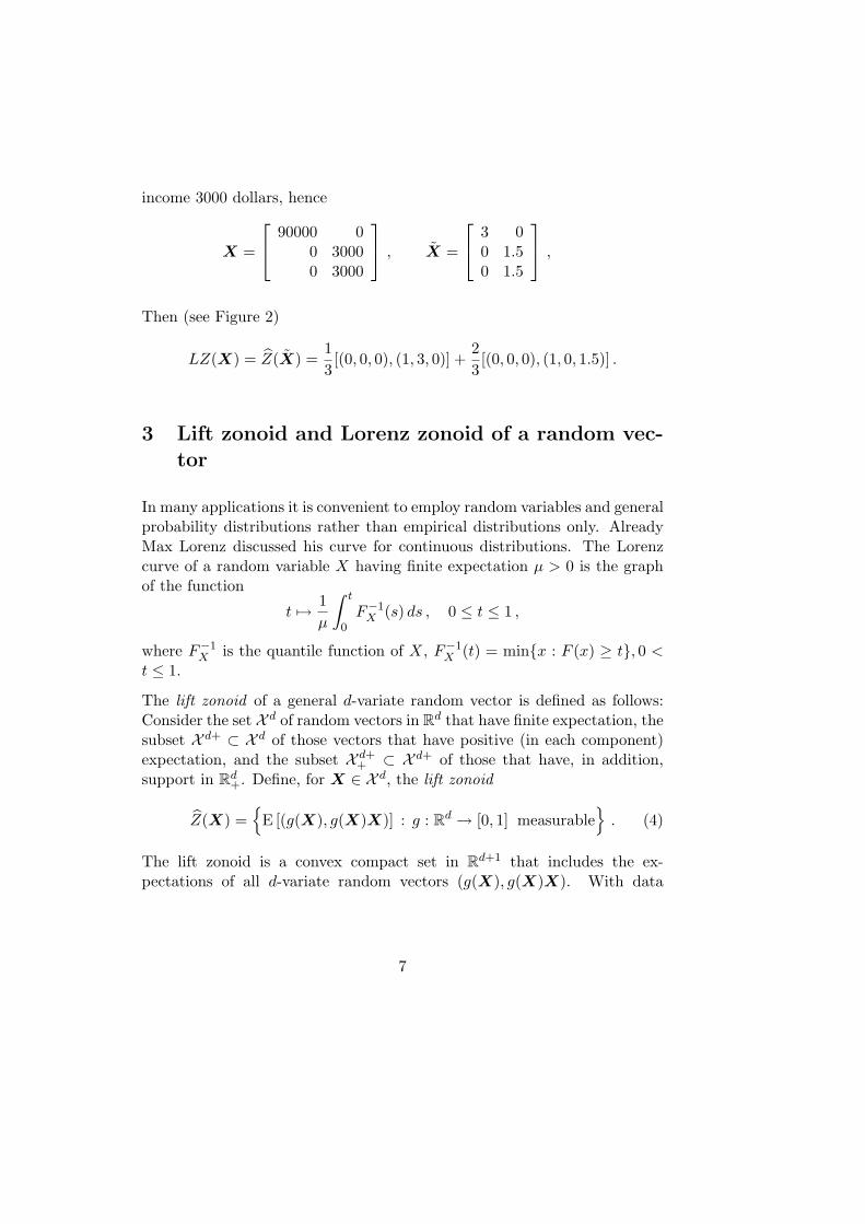
income 3000 dollars, hence

X =

90000 00 30000 3000

, X =

3 00 1.50 1.5

,

Then (see Figure 2)

LZ(X) = Z(X) =13[(0, 0, 0), (1, 3, 0)] +

23[(0, 0, 0), (1, 0, 1.5)] .

3 Lift zonoid and Lorenz zonoid of a random vec-tor

In many applications it is convenient to employ random variables and generalprobability distributions rather than empirical distributions only. AlreadyMax Lorenz discussed his curve for continuous distributions. The Lorenzcurve of a random variable X having finite expectation µ > 0 is the graphof the function

t 7→ 1µ

∫ t

0F−1

X (s) ds , 0 ≤ t ≤ 1 ,

where F−1X is the quantile function of X, F−1

X (t) = min{x : F (x) ≥ t}, 0 <t ≤ 1.

The lift zonoid of a general d-variate random vector is defined as follows:Consider the set X d of random vectors in Rd that have finite expectation, thesubset X d+ ⊂ X d of those vectors that have positive (in each component)expectation, and the subset X d+

+ ⊂ X d+ of those that have, in addition,support in Rd

+. Define, for X ∈ X d, the lift zonoid

Z(X) ={

E [(g(X), g(X)X)] : g : Rd → [0, 1] measurable}

. (4)

The lift zonoid is a convex compact set in Rd+1 that includes the ex-pectations of all d-variate random vectors (g(X), g(X)X). With data

7

X = (x1, . . . ,xn)′, the definition (4) of the lift zonoid specializes to theprevious one (3): By setting λi = 1

ng(xi) we see that

Z(X) =

{(n∑

i=1

λi,n∑

i=1

λixi

): 0 ≤ λi ≤ 1

n, i = 1, . . . , n

}

=1n

n∑

i=1

[(0,0), (1, xi)] .

The lift zonoid has many attractive properties, which make it useful for abroad range of applications. Here we mention only three of them. For proofsof the subsequent propositions and many more properties and applicationsthe reader is referred to [21] and the comprehensive monograph [32].

The first important property is uniqueness. Like the generalized Lorenzcurve in dimension one, the lift zonoid contains full information about theunderlying distribution, that is, given the lift zonoid, the data can be com-pletely regained.

Proposition 1 (Uniqueness). The lift zonoid Z(X) uniquely determinesthe distribution FX , for X ∈ X d.

The second property regards marginalization. If we restrict to one or severaldimensions of the data, the lift zonoid of the marginal distribution is a simpleprojection of the lift zonoid of the joint distribution:

Proposition 2 (Marginalization). For any J ⊂ {1, 2, . . . d} consider theprojection prJ : z 7→ (z0, zJ), z ∈ Rd+1, where zJ is the subvector containingcomponents zj , j ∈ J . Then

prJ(Z(X)) = Z(XJ) .

Thirdly, we state that the lift zonoid is additive in the distribution:

Proposition 3 (Additivity). For two random vectors X and Z in X d

with distributions FX and FZ and α ∈ [0, 1],

Z(αFX + (1− α)FZ) = αZ(FX) + (1− α)Z(FZ) .

8

For data X and Y , the last equation reads

Z(x1, . . . , xn, y1, . . . ,ym) =n

n + mZ(x1, . . . ,xn) +

m

n + mZ(y1, . . . ,ym) ,

(5)which is immediately seen from the definition (3). The additivity propertyis useful with indices based on the lift zonoid; it allows to decompose anindex into subgroups of the population.

Now, the general definition of the Lorenz zonoid of a random vector and itsproperties are straightforward ([18]). The Lorenz zonoid of some X ∈ X d+

is the lift zonoid of the relative vector, i.e. the vector componentwise dividedby its expectation. With

X =(

X1

E[X1], . . . ,

Xd

E[Xd]

)

define

LZ(X) = Z(X) ={

E[(

g(X), g(X)X)]

: g : Rd → [0, 1] measurable}

(6)The Lorenz zonoid of a random vector X ∈ X d+ is a convex compact set inRd+1. Moreover, if X ∈ X d+

+ , i.e., has support in Rd+, the Lorenz zonoid is

contained in the unit hypercube of Rd+1.

Economic interpretation of the Lorenz zonoid: The function g : Rd+ → [0, 1]

can be seen as a selection of some part of the population. Of all householdswhich have relative endowment vector X the percentage g(X) is selected.E[Xg(X)] amounts to the total portion vector held by this subpopulationand E[g(X)] is the size of the subpopulation selected by g.

The following three principal properties of the Lorenz zonoid correspond tothose of the lift zonoid.Uniqueness: The Lorenz zonoid of a random vector determines its distri-bution uniquely, up to d scale factors.Marginalization: The Lorenz zonoid of a marginal XJ is equal to theprojection of the Lorenz zonoid of X, for any J ⊂ {1, 2, . . . d}.For the third property, additivity, the Lorenz zonoids have to be rescaled,which is done by multiplying them pointwise with proper diagonal matrices:

9

Proposition 4 (Additivity). Given two random vectors X and Z in X d+

with distributions FX , FZ and some α ∈ [0, 1] consider a random vector Ythat has distribution FY = αFX + (1− α)FZ . Then2

LZ(Y ) = α LZ(X) diag(

1,E[X1]E[Y1]

, . . . ,E[Xd]E[Yd]

)

+ (1− α) LZ(Z) diag(

1,E[Z1]E[Y1]

, . . . ,E[Zd]E[Yd]

).

For proof, use Proposition 2.24 in [32]. More properties of the Lorenz zonoidare found in [18] and [32].

4 Lorenz dominance

Here we define multivariate Lorenz dominance via set inclusion of zonoids.We do this for general random vectors, which includes the case of multivari-ate data.

For two random vectors in X d define the Lorenz dominance ¹dL by

X ¹dL Y if LZ(X) ⊂ LZ(Y ) . (7)

As the Lorenz zonoid of a random vector depends on its distribution only,we also write FX ¹d

L FY in place of X ¹dL Y .

First consequences of the definition are: The Lorenz dominance ¹dL is

a preorder (reflexive and transitive) on X d+. Its smallest elements arethe constant random vectors, which correspond to egalitarian distribu-tions. The preorder is scale invariant, (X1, . . . , Xd) ¹d

L (Y1, . . . , Yd) implies(λ1X1, . . . , λdXd) ¹d

L (λ1Y1, . . . , λdYd) for any λ1, . . . , λd > 0.

When d = 1, the Lorenz zonoid is the area between the Lorenz curve and thedual Lorenz curve; thus the preorder reduces to the usual Lorenz dominance.

The following Proposition 5 characterizes the multivariate Lorenz dominanceby similar univariate dominances.

2diag(λ1, . . . , λd) denotes a matrix having elements λ1, . . . , λd in the diagonal and 0outside.

10

Proposition 5 (Characterization of Lorenz dominance). The follow-ing statements ar equivalent:(i) (X1, . . . , Xd) ¹d

L (Y1, . . . , Yd)

(ii) For every p = (p1, . . . , pd) ∈ Rd, the generalized Lorenz curve of

d∑

j=1

pj Yj lies above that ofd∑

j=1

pjXj .

(iii) For every convex function ψ : R→ R and p ∈ Rd,

E

ψ

d∑

j=1

pjXj

≤ E

ψ

d∑

j=1

pj Yj

. (8)

(iv) For every increasing3 convex function ψ : R → R and p ∈ Rd, (8) issatified.

(v) For every p ∈ Rd exists a random variable Up such thatE[Up|

∑dj=1 pjXj ] = 0 and

d∑

j=1

pj Yj =st

d∑

j=1

pjXj + Up . (9)

Here =st indicates equality in distribution. Part (ii) of the Proposition is alsocalled directional majorization of Y over X. See [5, 10]. It can be interpretedin terms of ‘prices’ and ‘expenditures’. When, with properly chosen units,the mean endowment of each commodity amounts to one and X and Ysignify alternative distributions of the commodity vector, then

∑dj=1 pjXj

and∑d

j=1 pj Yj stand for the distributions of expenditures given the pricevector p. The proposition says that X has less multivariate disparity thanY if and only if the first distribution of expenditures is less unequal thanthe second – in the sense of usual Lorenz dominance – for every price vectorin d-space. Note that this also includes negative prices. Later, in Section 6,we will discuss a related ordering that employs nonnegative prices only.

In terms of expected utility, Part (iv) of Proposition 5 means that everyrisk seeking person which has to choose between the random expenditures

3‘Increasing’ is always meant in the weak sense.

11

∑dj=1 pjXj and

∑dj=1 pj Yj will, for any prices, prefer the latter, and that

every risk averse person will do the opposite. Part (iii) says the same, withnot necessarily increasing utilities.

In Part (v), Up may be interpreted as a perturbation of expenditures or‘noise’. The distribution of expenditures for Y is, for all prices, ‘noisier’than the distribution of expenditures for X.

From the projection property we conclude: LZ(X) ⊂ LZ(Y ) impliesLZ(XJ) ⊂ LZ(Y J) for all J ⊂ {1, . . . d}. Hence Lorenz dominance of tworandom vectors implies Lorenz dominance of all subvectors. In particular,this holds for every single commodity:

Proposition 6 (Projection). If (X1, . . . , Xd) ¹dL (Y1, . . . , Yd) then

Xj ¹1L Yj for j = 1, . . . d.

But the following example demonstrates that the reverse implication is nottrue.

Example 4: Let d = 2, n = 3, and

X =

.25 .5

.25 .25

.5 .25

, Y =

1 10 00 0

.

Then Y Lorenz dominates X in each single attribute. But the dimensionof LZ(X) is 3, whereas the dimension of LZ(Y ) is 2. Therefore LZ(X) isno subset of LZ(Y ), and Y does not dominate X.

If the attributes are stochastically independent, a reverse implication holds.Then the multivariate Lorenz dominance is equivalent to the usual Lorenzdominance of the marginals:

Proposition 7. Assume that the components X1, . . . , Xd as well the compo-nents Y1, . . . , Yd are independent. Then X ¹d

L Y if and only if Xj ¹1L Yj

for all j = 1, . . . , d.

Finally we mention a result about random vectors with given marginals:One cannot dominate the other unless they have the same distribution.

Proposition 8 (Equal marginals). If the univariate marginal distribu-tions of two random vectors X and Y coincide, then

X ¹dL Y ⇒ FX = FY .

12

5 Scaled convex order

There are many possibilities to extend the classical Lorenz dominance tothe multivariate case. The Lorenz dominance introduced above is just oneof them. Another one is the multivariate scaled convex order, which is nowconsidered and contrasted with the Lorenz dominance.

Proposition 9 (Scaled convex order). For X, Y ∈ X d the followingstatements are equivalent:

(i) E[ψ(X)] ≥ E[ψ(Y )] if φ : Rd → R is concave and the expectations exist,

(ii) E[φ(X)] ≤ E[φ(Y )] if φ : Rd → R is convex and the expectations exist,

(iii) E[φ(X)] ≤ E[φ(Y )] if φ : Rd → R is increasing convex and the expec-tations exist,

(iv) Y =st X + U for some U with E[U |X] = 0.

X is said to be not larger than Y in scaled convex order, X ¹dscx Y , if

one of these equivalent restrictions is satisfied. The scaled convex order is apreorder on X d.

In economic terms, X ¹dscx Y means that, if welfare is evaluated by a util-

itarian social welfare function based on concave individual relative welfarefunctions, the distribution of X is always preferred over the distribution ofY .

Many results on the convex order are found in [38] and [35]. The randomvector U in Proposition 9(iv) can be interpreted as ‘noise’, so that Y isdistributed as X plus some noise.

In view of Propositions 5(iii) and 9(ii) and, as every convex-linear functionis convex, the scaled convex order implies the Lorenz dominance,

X ¹dscx Y ⇒ X ¹L Y . (10)

In case d = 1 the scaled convex order is the same as the Lorenz dominance.But for d ≥ 2 the two orderings coincide in special cases only.

Example 5 (Multivariate normal distributions): Among multivariatenormal distributions the two dominance relations are equivalent and char-acterized as follows:

13

Assume X ∼ N(a, R) and Y ∼ N(b,S) with covariance matrices R = [rij ],S = [sij ] and positive (in each component) mean vectors a = (a1, . . . , ad),b = (b1, . . . , bd). Then

X ¹dscx Y ⇔ X ¹d

L Y

⇔d∑

i=1

d∑

j=1

pipj

(sij

bibj− rij

aiaj

)≥ 0 for all p ∈ Rd ,

that is, the covariance matrix of Y is larger than that of X in the usualcovariance matrix ordering.

In view of Proposition 9(iv), checking data X and Y for scaled convex orderis a relatively simple task. It amounts to solving a linear program:

Proposition 10 (Checking for scaled convex order). Assume thatall rows xi of X are different, and the same for all rows yi of Y . ThenX ¹d

scx Y if and only there exists a bistochastic matrix Π = (πij) thatsatisfies

xi =n∑

j=1

πijyj , i = 1, . . . , n .

As scaled convex order implies Lorenz order, Proposition 10 provides a suf-ficient condition for X ¹d

L Y . A necessary condition has been given inProposition 6: the Lorenz ordering of all marginals.

6 Extended lift zonoids and price Lorenz domi-nance

Here we consider a new object, the Minkowski sum of the lift zonoid and acertain orthant of (d+1)-space. We call it the extended lift zonoid. Similarly,an extended Lorenz zonoid is introduced, which is the extended lift zonoidof the relative distribution. The boundary of the extended Lorenz zonoidcontains the Lorenz hypersurface.

The inclusion of these sets yields an ordering which has a similar characteri-zation as the Lorenz dominance (Proposition 5). In this, the set of all prices(or directions) is replaced by the set of all nonnegative prices.

14

In the rest of the paper assume that X and Y have support in Rd+, X, Y ∈

X d++ . To construct the extended lift zonoid eZ(X), the lift zonoid Z(X) is

augmented by all points that are below a point in Z(X) regarding the firstcoordinate and above the point regarding the other d coordinates. Moreprecisely,

eZ(X) = {(v0, v1, . . . , vd) : v0 ≤ z0, vj ≥ zj , j = 1, . . . , d ,

for some (z0, z1, . . . , zd) ∈ Z(X)}= Z(X) + (R− × Rd

+)

When using the relative random vector X we obtain the extended Lorenzzonoid,

eLZ(X) = eZ(X) . (11)

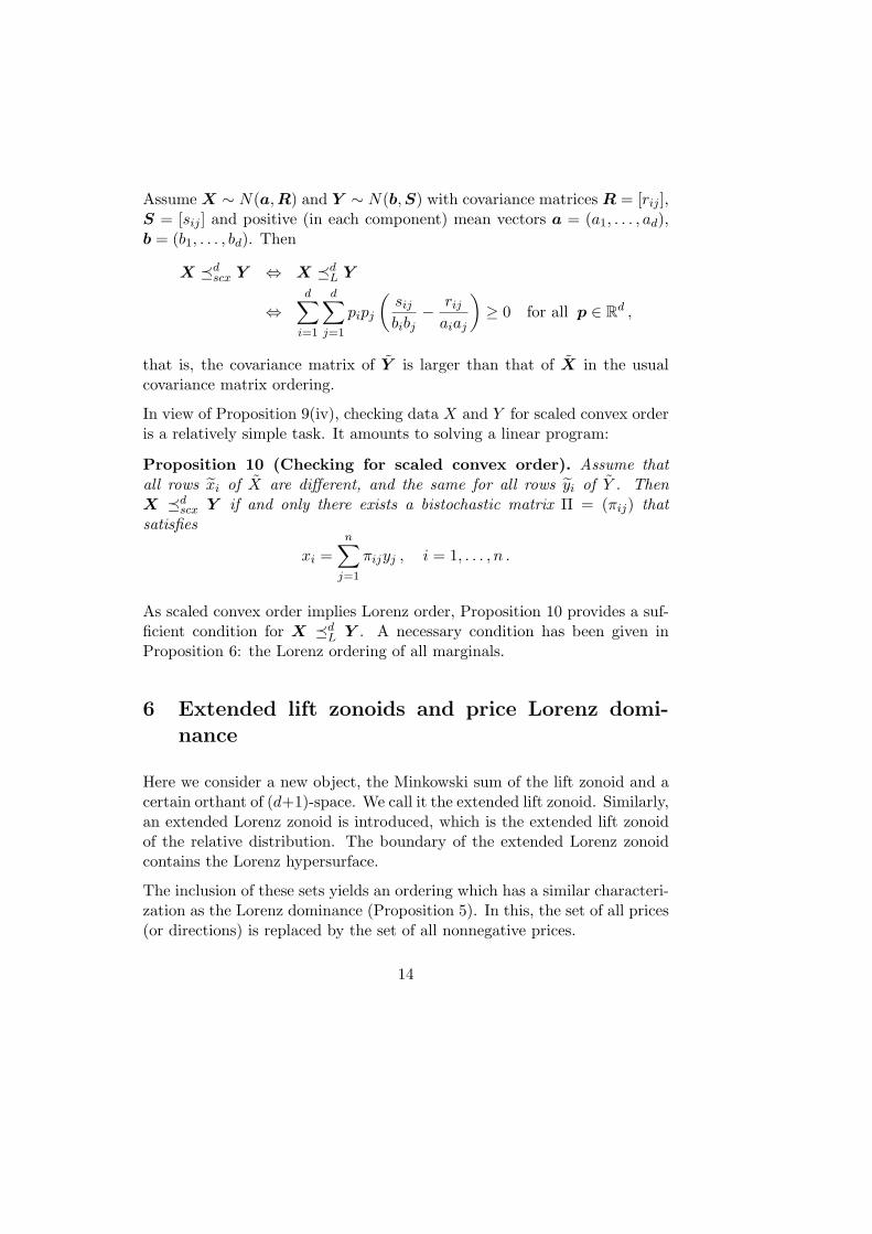
Figure 3 exhibits the extended Lorenz zonoid of a two-attribute egalitariandistribution.

The set inclusion of extended Lorenz zonoids provides an ordering,

X ¹dPL Y if eLZ(X) ⊂ eLZ(Y ) , (12)

which can be characterized as follows.

Proposition 11. The following statements ar equivalent:(i) X ¹d

PL Y

(ii) For every p = (p1, . . . , pd) ∈ Rd+,

the generalized Lorenz curve ofd∑

j=1

pj Yj lies above that ofd∑

j=1

pjXj .

(13)(iii) For every convex function ψ : R→ R and p ∈ Rd

+,

E

ψ

d∑

j=1

pjXj

≤ E

ψ

d∑

j=1

pj Yj

. (14)

(iv) For every increasing convex function ψ : R → R and p ∈ Rd+, (14) is

satified.

15

In view of Proposition 11, the ordering ¹dPL is named price Lorenz domi-

nance. The interpretation is that, for all nonnegative price vectors p, ex-penditures are less dispersed with X than with Y .

When d = 1, the extended Lorenz zonoid covers the plane south and eastof the Lorenz curve; it is included in another extended Lorenz zonoid if andonly if its Lorenz curve lies below the other Lorenz curve.

Similarly, for set inclusion of extended Lorenz zonoids in higher dimensions,only that parts of their boundaries are relevant that lie in the unit hypercubeof Rd+1. This part of the boundary is named the Lorenz hypersurface, insymbols

LH(X) = ∂eLZ(X) ∩ [0, 1]d+1 ,

where ∂S denotes the boundary of a set S. LH(X) is the graph of a functionlX which is called the inverse Lorenz function (ILF),

lX(y) = maxE[g(X)] , y ∈ [0, 1]d , (15)

where the maximum extends over all functions g : Rd+ → [0, 1] for which

E[g(X)X] ≤ y

holds in the usual componentwise order of Rd+1.

In particular, the ILF of an empirical distribution is a piecewise linear func-tion,

lX(y) = max

{n∑

i=1

λi :n∑

i=1

λixi ≤ y, 0 ≤ λi ≤ 1n

}, y ∈ [0, 1]d , (16)

and the Lorenz hypersurface is a piecewise linear hypersurface whose ex-treme points are solutions to a linear program.

In case d = 1 the ILF is the inverse function of the usual Lorenz func-tion. The Lorenz dominance between univariate distributions consists inthe pointwise ordering of their Lorenz functions or, equivalently, of theirILFs.

For general d, the ILF is defined on the unit cube of Rd. Its argument yrepresents a vector of relative endowments with respect to mean endowments

16

in the d attributes. lX(y) equals the maximum percentage of householdswho hold a vector of shares less than or equal to y = (y1, . . . , yd).

Example 6 (Egalitarian distribution): With X = Ec holds xi =(1, . . . , 1) for all i,

n∑

i=1

λixi =n∑

i=1

λi (1, . . . , 1) ≤ y ⇔ 0 ≤n∑

i=1

λi ≤ minj

yj .

Hence the ILF is

lEc(y) = minj

yj for y ∈ [0, 1]d ,

which does not depend on c. See also Figure 3.

Example 7 (Antiegalitarian distribution): An antiegalitarian distribu-tion Ac,i∗ gives all to one household i∗. E.g., with i∗ = 1,

Ac,1 =

c1 . . . cd

0 . . . 0. . .

0 . . . 0

.

Now let X = Ac,i∗ for some i∗. Then xi = (n, . . . , n) if i = i∗ and xi =(0, . . . , 0) otherwise,

n∑

i=1

λixi = λi∗(n, . . . , n) ≤ y

⇔ 0 ≤ λi∗ ≤ 1n

minj

yj and λi ≤ 1n

for i 6= i∗ .

HencelAc,i∗ (y) =

n− 1n

+1n

minj

yj for y ∈ [0, 1]d ,

independently of c and i∗.

Principal properties of the ILF are:

• lX is monotone increasing, concave, and has values in [0, 1],

• lX(1) = 1 , lX(0) = Pr[X ≤ 0] ,

17

• lX(yJ ,1−J) = lXJ(yJ).

Here, (yJ ,1−J) is the vector in Rd with components yj , j ∈ J, and remainingcomponents equal to 1.

The Lorenz hypersurface defines the underlying distribution uniquely, up toa vector of scale factors. It is additive in the distribution, and its properprojections form the Lorenz hypersurfaces of the marginals. For more prop-erties and details, see [22] and [32, ch.9].

7 Decomposition of the volume-Gini index

In the multivariate case, there are two interesting extensions of the usualGini index; see Koshevoy and Mosler [20]. One, called volume-Gini index, isbased on the definition of the univariate Gini index as the area between theLorenz curve and its symmetric curve, that is the area of the Lorenz zonoid.The volume-Gini index is essentially the volume of the Lorenz zonoid; seebelow. The second extension of the usual Gini index, called distance-Giniindex, uses the fact that this area equals the mean difference over the mean.In dimensions d ≥ 2 the two approaches lead to different indices.

An important question is, whether an index can be decomposed into indicesof subgroups of the population. Here, we will provide a decomposition ofthe volume-Gini mean difference, which is essentially the volume of the liftzonoid. The volume-Gini index, then, is the volume-Gini mean difference ofthe relative data. For this, we exploit the additivity property of lift zonoids.

Given X = (x1, . . . , xk) and Y = (y1, . . . , yl) consider the combined dataset X ∪ Y = (x1, . . . , xk, y1, . . . , yl). Then, by Proposition 3,

Z(X ∪ Y ) =k

k + lZ(X) +

l

k + lZ(Y ). (17)

Various indices that are based on lift or Lorenz zonoids can be decomposedby combining the additivity property with some version of Minkowski’s the-orem. For the Minkowski theorem (the Steiner decomposition indeed) andits variants, see [36].

18

The volume-Gini mean difference MV of a d-variate data set X is definedby (see [20])

MV (X) =1

2d − 1

(vol

(Z(X) + Cd

)− 1

),

where Cd = {(0, z1, . . . , zd) : 0 ≤ zi ≤ 1, i = 1, . . . , d} is a d-dimensional unitcube in Rd+1.

From Minkowski’s theorem we obtain a formula for the volume of (17):

vol(Z(X ∪ Y )) =(

k

k + l

)d+1

vol(Z(X)) +(

l

k + l

)d+1

vol(Z(Y ))

+d∑

m=1

(d + 1

m

)kmld+1−m

(k + l)d+1mixvolm(Z(X), Z(Y)). (18)

Here mixvolm(A,B) denotes the mixed volume of (A, . . . , A, B, . . . , B) withm repetitions of A and d+1−m repetitions of B. A formula similar to (18)holds true for MV ,

(2d + 1)MV (X ∪ Y ) + 1 = (19)(

k

k + l

)d+1

vol(Z(X) + Cd) +(

l

k + l

)d+1

vol(Z(Y ) + Cd)

+d∑

m=1

(d + 1

m

)kmld+1−m

(k + l)d+1mixvolm(Z(X) + Cd, Z(Y ) + Cd) .

We conclude:

Proposition 12.

MV (X ∪ Y ) =(

k

k + l

)d+1

MV (X) +(

l

k + l

)d+1

MV (Y )

+d∑

m=1

(d + 1

m

)kmld+1−m

(k + l)d+1

[mixvolm(Z(X) + Cd, Z(Y ) + Cd)− 1

].

For convex compacts K1, . . . , Kn in Rn, the mixed volume has a simpleexpression as an alternating sum of ordinary volumes:

mixvol(K1, . . . , Kn) =1n !

n∑

j=1

(−1)n−j∑

i1<···<ij

vol(Ki1 + . . . + Kij ) (20)

19

From this representation of the mixed volume it is seen thatmixvol(K1, . . . , Kn) is a symmetric, multilinear and equivariant (under lin-ear transformations) function of its variables. It holds mixvol(K, . . . , K) =vol(K). Moreover, the mixed volumes are monotone (which is a nontrivialresult):

mixvol(K ′1, . . . ,K

′n) ≤ mixvol(K1, . . . ,Kn) if K ′

i ⊂ Ki for all i .

If K1, . . . , Kd+1 are lift zonoids of probability distributions F1, . . . , Fd+1 inRd, a formula for their mixed volume is obtained from (20):

mixvol(K1, . . . , Kd+1) = (21)1

(d + 1)!

∫

Rd

· · ·∫

Rd

∣∣∣∣det(

1x1· · · 1

xd+1

)∣∣∣∣ dF1(x1) . . . dFd+1(xd+1) .

Now, consider the case d = 1. By (20) the mixed volume of two convexcompact sets in R2 is given as

mixvol(K,L) =12(vol(K + L)− vol(K)− vol(L)) . (22)

Further, for univariate data X = (x1, . . . , xk), Y = (y1, . . . , yl), it holdsvol(Z(X) + C1) = vol(Z(X)) + 1 and vol(Z(X) + C1 + Z(Y ) + C1) =vol(Z(X) + Z(Y )) + 4, hence, by (22), mixvol(Z(X) + C1, Z(Y ) + C1) =mixvol(Z(X), Z(Y )) + 1. From (21) we obtain

mixvol(Z(X), Z(Y )) =12

1kl

k∑

i=1

l∑

j=1

|yj − xi| ,

and Proposition 12 yields the following three-term decomposition of thevolume-Gini mean difference:

MV (X ∪ Y ) =(

k

k + l

)2

MV (X) +(

l

k + l

)2

MV (Y ) (23)

+1

(k + l)2

k∑

i=1

l∑

j=1

|yj − xi| .

Another decomposition of MV can be obtained from Theorem 5.2 ([20]) and(21). The details of this decomposition are left to the reader.

20

In dimension d > 1 more than three terms in the decomposition of thevolume-Gini mean difference do appear. Note that the distance-Gini index([20]) has, for any dimension d, a three-term decomposition similar to (23).

Let us note that Minkowski type theorems hold for other characteristics,say the surface area, of convex sets, too. Again, consider univariate dataand observe (22). Let B denote the unit disc in R2. Then, 2 ·mixvol(K, B)amounts to the circumference of K. For the unit segment S in direction p,2 ·mixvol(K, S) is the width of K in the direction orthogonal to p. By this,for univariate data, the additivity of the length of the Lorenz curve can beestablished.

8 Final remarks

Several multivariate generalizations of classical Lorenz curve and orderinghave been surveyed in this paper. The key notions were the lift zonoidand the Lorenz zonoid of a d-variate distribution, and the graph of theinverse Lorenz function, which is part of the Lorenz zonoid’s boundary. Inparticular, the pointwise ordering of inverse Lorenz functions is equivalent tothe price Lorenz dominance. The Lorenz hypersurface is visual in the sameway as the usual Lorenz curve is: increasing deviation from the egalitarianhypersurface indicates more disparity. The Lorenz hypersurface defines theunderlying distribution uniquely, up to a vector of scaling constants.

As Lorenz did, the above analysis regards distributions of relative endow-ments. Similar dominance relations can be considered for distributions ofabsolute endowments; see [21, 32]. Like usual Lorenz dominance correspondsto vector majorization, these relations correspond to super- and subma-jorization.

The lift zonoid provides an embedding of d-variate distributions into theconvex compacts of (d + 1)-space. This embedding has attractive analyticalproperties and opens a special, visual way to the investigation of multivariatedistributions. The distributions can be fully described by zonoid data depthand zonoid central regions, which arise from d-dimensional cuts of the liftzonoid ([19, 7]). The approach lends itself not only to measuring disparity,as we did it here in the tradition of Lorenz, but also to compare distributionswith respect to location and dependency ([33]). Zonoid central regions may

21

also be employed to exclude outlying data and to restrict Lorenz dominanceto central parts of the distributions ([34]). Moreover, the lift zonoid is relatedin a visual way to other notions of data depth like the Oja depth and theTukey depth ([17]). Also, statistical inference has been based on the zonoiddata depth: testing for location and scale ([6]), testing on dependency ([25]),and estimating a scatter matrix ([24]).

Beyond probability distributions in Rd, the lift zonoid of a capacity and theordering induced by it has been discussed in [16].

For future research on measuring multidimensioned economic inequality fourtopics appear to be most relevant: (1) relations that are weaker (implied by)multivariate Lorenz dominance, (2) postulates for indices and dominancerelations that model interaction effects between attributes, (3) subgroupdecompositions of indices that allow an economic interpretation, (4) com-putational issues.

References

[1] Alker, H.: Mathematics and Politics. MacMillan, New York 1965.

[2] Atkinson, A.: On the measurement of inequality. Journal of EconomicTheory 2 (1970), 244–263.

[3] Atkinson, A., and Bourguignon, F.: The comparison of multidimen-sioned distributions of economic status. Review of Economic Studies29 (1982), 183–201.

[4] Atkinson, A., and Bourguignon, F.: The design of direct taxation andfamily benefits. Journal of Public Economics 41 (1989), 3–29.

[5] Bhandari, S.K.: Multivariate majorization and directional majoriza-tion: Positive results. Sankhya A 50 (1988), 199–204.

[6] Dyckerhoff, R.: Inference based on data depth. 2002. Chapter 5 in [32].

[7] Dyckerhoff, R., Koshevoy, G., and Mosler, K.: Zonoid data depth: The-ory and Computation. In COMPSTAT 1996 (A. Prat, ed.). Physica-Verlag, Heidelberg 1996, pp 235–240.

22

[8] Goldie, C.: Convergence theorems for empirical Lorenz curves and theirinverses. Advances in Applied Probability Theory 9 (1977), 765–791.

[9] Hart, P., Entropy and other measures of concentration. Journal of theRoyal Statistical Society, Series A 134 (1971), 73–89.

[10] Joe, H., and Verducci, J.: Multivariate majorization by positive com-binations. In Stochastic Inequalities (M. Shaked and Y.L. Tong, eds.).IMS, Hayward 1992, pp 159–181.

[11] Kolm, S.C.: The optimal production of social justice. In Public Eco-nomics (J. Marjolis and H. Guitton, eds.). Macmillan, New York 1969,pp 145–200.

[12] Kolm, S.C.: Multidimensional egalitarianisms. Quarterly Journal ofEconomics 91 (1977), 1–13.

[13] Koshevoy, G.: Multivariate inequality indices and orderings on a prod-uct of symmetric groups. Economica i Matematicheskie Methody 29(1993), 245-256 (in Russian).

[14] Koshevoy, G.: Multivariate Lorenz majorization. Social Choice andWelfare 12 (1995), 93-102.

[15] Koshevoy, G.: The Lorenz zonotope and multivariate majorizations,Social Choice and Welfare 15 (1998), 1–14.

[16] Koshevoy, G.: Orderings of capacities. Lecture at the Bocconi Univer-sity, Milano, May 2002

[17] Koshevoy, G.: Lift zonoid and multivariate depths. In: Developmentsin Robust Statistics (Eds. R. Dutter et al.). Physica-Verlag, Heidelberg(2003), pp 193–201.

[18] Koshevoy, G., and Mosler, K.: The Lorenz zonoid of a multivariatedistribution, Journal of the American Statistical Association 91 (1996),873–882.

[19] Koshevoy, G., and Mosler, K.: Zonoid trimming for multivariate distri-butions. The Annals of Statistics 25 (1997), 1998–2017.

23

[20] Koshevoy, G., and Mosler, K.: Multivariate Gini indices, Journal ofMultivariate Analysis 60 (1997), 252–276.

[21] Koshevoy, G., and Mosler, K.: Lift zonoids, random convex hulls andthe variability of random vectors. Bernoulli 4 (1998), 377–399.

[22] Koshevoy, G., and Mosler, K.: Price majorization and the inverseLorenz function. Discussion Papers in Statistics and Econometrics 3(1999), Universitat zu Koln.

[23] Koshevoy, G., and Mosler, K.: Measuring multidimensional concen-tration: A geometrical approach. Allgemeines Statistisches Archiv 83(1999), 173–188.

[24] Koshevoy, G., Mottonen, J., and Oja, H.: A scatter matrix estimatebased on zonotope. The Annals of Statistics 31 (2003), 1439–1459.

[25] Koshevoy, G., Mottonen, J., Oja, H., and Tyurin, Y.: Dependency testsbased on zonotopes (2005). Submitted.

[26] Maasoumi, E.: The measurement and decomposition of multidimen-sional inequality. Econometrica 54 (1986), 991–997.

[27] Lorenz, M.O.: Methods of measuring the concentration of wealth, Pub-lication of the American Statistical Association 9 (1905), 209–219.

[28] Mosler, K. and Scarsini, M.: Stochastic Orders and Applications. AClassified Bibliography. Springer, Berlin 1993.

[29] Mosler, K.: Majorization in economic disparity measures. Linear Alge-bra and Its Applications 199 (1994), 91–114. Correction: 220, 3.

[30] Mosler, K.: Multidimensional welfarisms. In Models and Measurementof Welfare and Inequality (W. Eichhorn, ed.). Springer, Berlin 1994,pp. 808–820.

[31] Mosler, K.: Multidimensional indices and orders of diversity. Commu-nity Ecology 2 (2001), 137–143.

[32] Mosler, K.: Multivariate Dispersion, Central Regions and Depth: TheLift Zonoid Approach. Springer, New York 2002.

24

[33] Mosler, K.: Central regions and dependency Methodology and Comput-ing in Applied Probability 5 (2003), 5–21.

[34] Mosler, K.: Restricted Lorenz dominance of economic inequality in oneand many dimensions Journal of Economic Inequality 2 (2004), 89–103.

[35] Muller, A. and Stoyan, D.: Comparison Methods for Stochastic Modelsand Risk. J. Wiley, New York 2002.

[36] Schneider, R. (1993): Convex Bodies: The Brunn-Minkowski Theory.Cambridge, Cambridge University Press.

[37] Sen, A.K.: On Economic Inequality. Oxford University Press 1973.

[38] Shaked, M. and Shanthikumar, J.G.: Stochastic Orders and Their Ap-plications. Academic Press, Boston 1994.

[39] Tsui, K.: Multidimensional generalizations of the relative and abso-lute inequality indices: The Atkinson-Kolm-Sen approach. Journal ofEconomic Theory 67 (1995), 251–265.

25

(a) Lorenz zonoid

0.5 1.0z1

0.5

1.0

z0

t

t

t

t

.......................................................................................................................................................................................................................................................................................................................................................................................................................................................................................................................................................................................................................................................................................................................................................................................................................................................

..... . .. . .. . .. . .. . .. . . . .. . . . .. . . . .. . . . .. . . . .. . . . . . .. . . . . . .. . . . . . .. . . . . . .. . . . . . .. . . . . . . . .. . . . . . . . .. . . . . . . . .. . . . . . . . .. . . . . . . . .. . . . . . . . . . .. . . . . . . . . . .. . . . . . . . .. . . . . . . . .. . . . . . . . .. . . . . . . . .. . . . . . . . .. . . . . . .. . . . . . .. . . . . . .. . . . . . .. . . . . . .. . . . .. . . . .. . . . .. . . . .. . . . .. . .. . .. . .. . .. . ..

....

................................................................................................................................................................................................................................ ............. ............. ............. ............. ............. ............. ............. ............. ............. ............. ............................................................................................................................................................qqqqqqqqqqqqqqqqqqqqqqqqq

qqqqqqqqqqqqqqqqqqqqqqqqqqqqqqqqqqqqqqqqqqqqqqqqqqqqqqqqqqqqqqqqqqqqqqqqqqqqqqqqqqqqqqqqqqqqqqqqqqqqqqqqqqqqqqqqqqqqqqqqqqqqqqqqqqqqqqqqqqqqqqqqqqqqqqqqqqqq

qqqqqqqqqqqqqqqqqqqqqqqqqqqqqqqqqqqqqqqqqqqqqqqqqqqqqqqqqqqqqqqqqqqqqqqqqq



qqqqqqqq

(b) Lift zonoid

2000 4000

0.5

1.0

z0

z1t

t

t

t

......................................................................................................................................................................................................

................................

................................

................................

................................

................................

................................

................................

................................

............................................................................................................................................................................................................................................................................................................................................................................................................................................................................................... .. .. . .. . .. . .. . . .. . . . .. . . . .. . . . . .. . . . . .. . . . . . .. . . . . . .. . . . . . .. . . . . . . .. . . . . . . . .. . . . . . . . .. . . . . . . . . .. . . . . . . . . .. . . . . . . . . . .. . . . . . . . . . .. . . . . . . . . . .. . . . . . . . . . . .. . . . . . . . . . . . .. . . . . . . . . . . . .. . . . . . . . . . . .. . . . . . . . . . . .. . . . . . . . . . .. . . . . . . . . . .. . . . . . . . . . .. . . . . . . . . .. . . . . . . . .. . . . . . . . .. . . . . . . .. . . . . . . .. . . . . . .. . . . . . .. . . . . . .. . . . . .. . . . .. . . . .. . . .. . . .. . .. . .. . .. ..

.

..........................

..........................

..........................

..........................

..........................

..........................

..........................

..........................

..........................

................... ............. ............. ............. ............. ............. ............. ............. ............. ............. ............. ............. ............. ............. ............................................................................................................................................................qqqqqqqqqqqqqqqqqqqqqqqqqqq

qqqqqqqqqqqqqqqqqqqqqqqqqqqqqqqqqqqqqqqqqqqqqqqqqqqqqqqqqqqqqqqqqqqqqqqqqqqqqqqqqqqqqqqqqqqqqqqqqqqqqqqqqqqqqqqqqqqqqqqqqqqqqqqqqqqqqqqqqqqqqqqqqqqqqqqqqqqqqqqqqqqqqqqqqq

qqqqqqqqqqqqqqqqqqqqqqqqqqqqqqqqqqqqqqqqqqqqqqqqqqqqqqqqqqqqqqqqqqqqqqqqqqqqqqqqqqqqqq



qqqqqqqqqq

Figure 1: (a) Lorenz curve and Lorenz zonoid LZ(2400, 5600), (b) gen-

eralized Lorenz curve and lift zonoid Z(2400, 5600) of the univariatetwo-point distribution in Example 1.

26

1- z1

1

6z0

................................

................................

................................

................................

................................

................................

................................

................................

................................

................................

................................

................................

................................

................................

................................

........1 z2

1

t

t

t

t

.................

..

..

..

..

..

..

.

..

..

..

.

..

..

..

..

.

..

..

..

..

.

..

..

..

..

..

..

..

..

..

..

.

..

..

..

..

..

..

..

..

..

..

..

..

..

..

..

..

..

..

..

..

..

..

..

..

..

..

..

..

..

..

..

..

..

.

..

..

..

..

..

..

..

.

..

..

..

..

..

..

..

..

.

..

..

..

..

..

..

..

..

.

..

..

..

..

..

..

..

..

..

..

..

..

..

..

..

..

..

..

.

..

..

..

..

..

..

..

..

..

..

..

..

..

..

..

..

..

..

..

..

..

..

..

..

..

..

..

..

..

..

..

..

..

..

..

..

..

..

..

..

..

..

..

..

..

..

..

..

..

..

..

..

..

.

..

..

..

..

..

..

..

..

..

..

..

..

..

..

..

..

..

..

..

..

..

..

..

..

.

..

..

..

..

..

..

..

..

..

..

..

..

.

..

..

..

..

..

..

..

..

..

..

..

..

..

.

..

..

..

..

..

..

..

..

..

..

..

..

..

.

..

..

..

..

..

..

..

..

..

..

..

..

..

..

..

..

..

..

..

..

..

..

..

..

..

..

..

..

.

..

..

..

..

..

..

..

..

..

..

..

..

..

..

..

..

..

..

..

..

..

..

..

..

..

..

..

..

..

..

..

..

..

..

..

..

..

..

..

..

..

..

..

..

.

..

..

..

..

..

..

..

..

..

..

..

..

..

..

..

..

..

..

..

..

..

..

..

..

..

..

..

..

..

..

..

..

..

..

..

..

..

..

..

..

..

..

..

..

.

..

..

..

..

..

..

..

..

..

..

..

..

..

..

..

..

..

..

..

..

..

..

..

..

..

..

..

..

..

..

..

..

..

..

..

..

..

..

..

..

..

..

..

..

.

..

..

..

..

..

..

..

..

..

..

..

..

..

..

..

..

..

..

..

..

..

..

..

..

..

..

..

..

..

..

..

..

..

..

..

..

..

..

..

..

..

..

..

..

..

..

..

..

..

..

..

..

..

..

..

..

..

..

..

..

..

..

..

..

..

..

..

..

..

..

..

..

..

..

..

..

..

..

..

..

..

..

..

..

..

..

..

..

..

..

..

..

..

..

..

..

..

..

..

..

..

..

..

..

..

..

..

..

..

..

..

..

..

..

..

..

..

..

..

..

..

..

..

..

..

..

..

..

..

..

..

..

..

..

..

..

..

..

..

..

..

..

..

..

..

..

..

..

..

..

..

..

..

..

..

..

..

..

..

..

..

..

..

..

..

..

..

..

..

..

..

..

..

..

..

..

..

..

..

..

..

..

..

..

..

..

..

..

..

..

..

..

..

..

..

..

..

..

..

..

..

..

..

..

..

..

..

..

..

..

..

..

..

..

..

..

..

..

..

..

..

..

..

..

..

..

..

..

..

..

..

..

..

..

..

..

..

..

..

..

..

..

..

..

..

..

..

..

..

..

..

..

..

..

..

..

..

..

..

..

..

..

..

..

..

..

..

..

..

..

..

..

..

..

..

..

..

..

..

..

..

..

..

..

..

..

..

..

..

..

..

..

..

..

..

..

..

..

..

..

..

..

..

..

..

..

..

..

..

..

..

..

..

..

..

..

..

..

..

..

..

..

..

..

..

..

..

..

..

..

..

..

..

..

..

..

..

..

..

..

..

..

..

..

..

.

..

..

..

..

..

..

..

..

..

..

..

..

..

..

..

..

..

..

..

..

..

..

..

..

..

..

..

..

..

..

..

..

..

..

..

..

..

..

..

..

..

..

..

..

..

.

..

..

..

..

..

..

..

..

..

..

..

..

..

..

..

..

..

..

..

..

..

..

..

..

..

..

..

..

..

..

..

..

..

..

..

..

..

..

..

..

..

..

..

..

..

..

..

..

..

..

..

..

..

..

..

..

..

..

..

..

..

..

..

..

..

..

..

..

..

..

..

..

..

..

..

..

..

..

..

..

..

..

..

..

..

..

.

..

..

..

..

..

..

..

..

..

..

..

..

..

..

..

..

..

..

..

..

..

..

..

..

..

.

..

..

..

..

..

..

..

..

..

..

..

..

.

..

..

..

..

..

..

..

..

..

..

..

.

..

..

..

..

..

..

..

..

..

..

..

.

..

..

..

..

..

..

..

..

..

..

..

..

..

..

..

..

..

..

..

..

..

..

..

..

..

..

..

..

..

..

..

..

..

..

..

..

..

..

..

..

..

.

..

..

..

..

..

..

..

..

..

.

..

..

..

..

..

..

..

..

.

..

..

..

..

..

..

..

..

.

..

..

..

..

..

..

..

..

..

..

..

..

..

..

..

.

..

..

..

..

..

..

..

..

..

..

..

..

..

..

..

..

..

..

..

..

..

..

..

..

..

..

..

..

..

..

..

.

..

..

..

..

..

..

..

..

..

.

..

..

..

..

.

..

..

..

.

..

..

..

.

..

..

..

..

..

..............

.......................................................................................................................................................................................................................................................................................................................

............................................

............................................

............................................

............................................

............................................

.....................................................................................................................................................................................................................................................................................................................................................................................................................................................................................................................................................................................................................

pppppppppppppppppppppppppppppppppppppppppppppppppppppppppppppppppppppppppppppppppppppppppppppppppppppppppppppppppppppppppppppppppppppppppppppppppppppppppppppppppppppppppppppppppppppppppppppppppppppppppppppppppppppppppppppppppppppppppppppppppppppppppppppppppppppppppppppppppppppppppppppppppppppppppppppppppppppppppppppppppppppppppppppppppppppppppppppppppppppppppppppppppppppppppppppppppppppppppppppppppppppppppppppppppppppppppppppppppppppppppppppppppppppppppppppppppppppppppppppppppppppppppppppppppppppppppppppppppppppppppppppppppppppppppppppp

pppppppppppppppppppppppppppppppppppppppppppppppppppppppppppppppppppppppppppppppppppppppppppppppppppppppppppppppppppppppppppppppppppppppppppppppppppppppppppppppppppppppppppppppppppppppppppppppppppppppppppppppppppppppppppppppppppppppppppppppppppppppppppppppppppppppppppppppppppppppppppppppppppppppppppppppppppppppppppppppppppppppppppppppppppppppppppppppppppppppppppppppppppppppppppppppppppppppppppppppppppppppppppppppppppppppppppppppppppppppppppppppppppppppppppppppppppppppppppppppppppppppppppppppppppppppppppppppppppppppppppppppppppppppppppppp

pppppppppppppppppppppppppppppppppppppppppppppppppppppppppppppppppppppppppppppppppppppppp

ppppppppppppppppppppppppppppppppppppppppppppppppppppppppppppppppppppppppppppppppppppppppppppppppppppppppppppppppppppppppppppppppppppppppppppppppppppppppppppppppppppppppppppppppppppppppppppppppppppppppppppppppppppppppppppppppppppppppppppppppppppppppppppppppppppppppppppppppppppppppppppppppppppppppppppppppppppppppppppppppppppppppppppppppppppppppppppppppppppppppppppppppppppppppppppppppppppppppppppppppppppppppppppppppppppppppppppppppppppppppppppppppppppppppppppppp

pppppppppppppppppppppppppppppppppppppppppppppppppppppppppppppppppppppppppppppppppppppppppppppppppppppppppppppppppppppppppppppppppppppppppppppppppppppppppppppppppppppppppppppppppppppppppppppppppppppppppppppppppppppppppppppppppppppppppppppppppppppppppppppppppppppppppppppppppppppppppppppppppppppppppppppppppppppppppppppppppppppppppppppppppppppppppppppppppppppppppppppppppppppppppppppppppppppppppppppppppppppppppppppppppppppppppppppppp

pppppppppppppppppppppppppppppppppppppppppppppppppppppppppppppppppppppppppppppp

pppppppppppppppppppppppppppppppppppppppppppppppppppppppppppppppppppppppppppppppppppppppppppppppppppppppppppppppppppppppppppppppppppppppppppppppppppppppppppppppppppppppppppppppppppppppppppppppppppppppppppppppppppppppppppppppppppppppppppppppppppppppppppppppppppppppppppppppppppppppppppppp

Figure 2: Lorenz zonoid of bivariate data. See Example 3.

...............................................................................................................................................................................................................................................................................................................................................................

........

........

........

........

........

........

........

........

........

........

........

........

........

........

........

........

........

........

........

........

........

........

........

........

........

........

........

........

........

........

........

........

........

........

........

........

........

........

........

........

........

........

........

........

........

........

........

........

........

........

........

........

.......

..........................................................................................................................................................................................................................................................................................................................................................................

.......

.

.

.

.

.

.

.

.

.

.

.

.

.

.

.

.

.

.

.

.

.

.

.

.

.

.

.

.

.

.

.

.

.

.

.

.

.

.

.

.

.

.

.

.

.

.

.

.

.

.

.

.

.

.

.

.

.

.

.

.

.

.

.

.

.

.

.

.

.

.

.

.

.

.

.

.

.

.

.

.

.

.

.

.

.

.

.

.

.

.

.

.

.

.

.

.

.

.

.

.

.

.

.

.

.

.

.

.

.

.

.

.

.

.

.

.

.

.

.

.

.

.

.

.

.

.

.

.

.

.

.

.

.

.

.

.

.

.

.

.

.

.

.

.

.

.

.

.

.

.

.

.

.

.

.

.

.

.

.

.

.

.

.

.

.

.

.

.

.

.

.

.

.

.

.

.

.

.

.

.

.

.

.

.

.

.

.

.

.

.

.

.

.

.

.

.

.

.

.

.

.

.

.

.

.

.

.

.

.

.

.

.

.

.

.

.

.

.

.

.

.

.

.

.

.

.

.

.

.

.

.

.

.

.

.

.

.

.

.

.

.

.

.

.

.

.

.

.

.

.

.

.

.

.

.

.

.

.

.

.

.

.

.

.

.

.

.

.

.

.

.

.

.

.

.

.

.

.

.

.

.

.

.

.

.

.

.

.

.

.

.

.

.

.

.

.

.

.

.

.

.

.

.

.

.

.

.

.

.

.

.

.

.

.

.

.

.

.

.

.

.

.

.

.

.

.

.

.

.

.

.

.

.

.

.

.

.

.

.

.

.

.

.

.

.

.

.

.

.

.

.

.

.

.

.

.

.

.

.

.

.

.

.

.

.

.

.

.

.

.

.

.

.

.

.

.

.

.

.

.

.

.

.

.

.

.

.

.

.

.

.

.

.

.

.

.

.

.

.

.

.

.

.

.

.

.

.

.

.

.

.

.

.

.

.

.

.

.

.

.

.

.

.

.

.

.

.

.

.

.

.

.

.

.

.

.

.

.

.

.

.

.

.

.

.

.

.

.

.

.

.

.

.

.

.

.

.

.

.

.

.

.

.

.

.

.

.

.

.

.

.

.

.

.

.

.

.

.

.

.

.

.

.

.

.

.

.

.

....

..

........

..

..

..

..

..

.

..

..

..

..

..

..

..

..

..

..

..

..

..

..

..

..

..

.

..

..

..

..

..

..

..

..

..

..

..

..

..

..

..

..

..

..

..

..

..

..

..

..

..

.

..

..

..

..

..

..

..

..

..

..

..

..

..

..

..

..

..

..

..

..

..

..

..

..

..

..

..

..

..

..

..

..

..

..

..

..

..

..

..

..

..

..

..

..

..

..

..

..

..

..

.

..

..

..

..

..

..

..

..

..

..

..

..

..

..

..

..

..

..

..

..

.

..

..

..

..

..

..

..

..

..

..

..

..

..

..

..

..

..

..

..

..

..

..

.

..

..

..

..

..

..

..

..

..

..

..

..

..

..

..

..

..

..

..

..

..

..

..

..

..

..

..

..

..

..

..

..

..

..

..

..

..

..

..

..

..

..

..

..

..

..

..

..

..

.

..

..

..

..

..

..

..

..

..

..

..

..

..

..

..

..

..

..

..

..

..

..

..

..

..

..

..

..

..

..

..

..

..

..

..

..

..

..

..

..

..

..

..

..

..

..

..

..

..

..

..

..

..

..

..

..

..

..

..

..

..

..

..

..

..

..

..

..

..

..

..

..

..

..

..

..

..

..

..

..

..

..

..

..

..

..

..

..

..

..

..

..

..

..

..

..

..

..

..

..

..

..

..

..

..

..

..

..

..

..

..

..

..

..

..

..

..

..

..

..

..

..

..

..

..

..

..

..

..

.

..

..

..

..

..

..

..

..

..

..

..

..

..

..

..

..

..

..

..

..

..

..

..

..

..

..

..

..

..

..

..

..

..

..

..

..

..

..

..

..

..

..

..

..

..

..

..

..

..

..

..

..

..

..

..

..

..

..

..

..

..

..

..

..

..

..

..

..

..

.

..

..

..

..

..

..

..

..

..

..

..

..

..

..

..

..

..

..

..

..

..

.

..

..

..

..

..

..

..

..

..

..

..

..

..

..

..

..

..

..

..

..

..

..

..

..

..

..

..

..

..

..

..

..

..

..

..

..

..

..

..

..

..

..

..

..

..

..

..

..

..

..

..

..

..

..

..

..

..

..

..

..

.

..

..

..

..

..

..

..

..

..

..

..

..

..

..

..

..

..

..

..

..

..

..

..

..

..

..

..

..

..

..

..

..

..

..

..

..

..

..

..

..

..

..

..

..

..

..

..

..

..

..

..

..

..

..

..

..

..

..

..

..

..

..

..

..

..

..

..

..

..

..

.

..

..

..

..

..

..

..

..

..

..

..

..

..

..

..

..

..

..

..

..

..

..

..

..

..

..

..

..

..

..

..

..

..

..

..

..

..

..

..

..

..

..

..

..

..

.

..

..

..

..

..

..

..

..

..

..

..

..

..

.

..

..

..

..

..

..

..

..

..

..

..

..

.

..

..

..

..

..

..

..

..

..

..

..

..

..

..

..

..

..

..

..

..

..

..

..

.

..

..

..

..

..

..

..

..

..

..

.

..

..

..

..

..

..

..

..

..

.

..

..

..

..

..

..

..

..

.

..

..

..

..

..

..

..

..

.

..

..

..

..

..

..

..

.

..

..

..

..

..

..

.

..

..

..

..

..

.

..

..

..

..

.

..

..

..

..

.

..

..

..

.

..

..

.

..

...

6

©©©©©©©©©©©©©©©*

@@

@@

@@

@@I

11

1

lEc(y1, y2)

y1y2

Figure 3: Lorenz hypersurface of a two-variate egalitarian distribu-tion

27

Multivariate Lorenz dominance based on zonoids

Documents

Transcript of Multivariate Lorenz dominance based on zonoids