DEPARTMENTOFECONOMICSANDFINANCE

DISCUSSIONPAPER2012‐09

MehmetPinar

ThanasisStengos

NikolasTopaloglou

JUNE,2012

CollegeofManagementandEconomics|GuelphOntario|Canada|N1G2W1

www.uoguelph.ca/economics

Measuringhumandevelopment:astochasticdominanceapproach

Measuring human development: a stochastic dominance

approach

Mehmet Pinar

University of Guelph∗Thanasis Stengos

University of Guelph†

Nikolas Topaloglou

Athens University of Economics and Business‡

February 2012

Abstract

We consider a weighting scheme that yields the best-case scenario measurement of theHuman Development Index (HDI) using an approach that relies on consistent tests forstochastic dominance efficiency (SDE). We compare a given hybrid composite indexsuch as the official equally-weighted HDI to all possible indices constructed from a set ofindividual components to obtain the most optimistic scenario for development. In thebest-case scenario index education is weighted considerably more than the other twocomponents, per capita income and life expectancy, relative to the weight that it getsin the official equally-weighted index. We find that the best-case scenario hybrid indexleads to a marked improvement of measured development over time when comparedwith the official equally-weighted HDI.

EL Classifications: C12; C13, C15; O15; O57Key Words: Nonparametric Stochastic Dominance; Human Development Index;

Mixed Integer Programming

∗Department of Economics, University of Guelph, N1G 2W1, Guelph, Ontario; e-mail: mp-inar@uoguelph.ca

†Department of Economics, University of Guelph, N1G 2W1, Guelph, Ontario; e-mail: tsten-gos@uoguelph.ca

‡Department of International European & Economic Studies, 76, Patision Street, GR10434, Athens;e-mail: nikolas@aueb.gr

1 Introduction

It has been recognized that welfare analysis based on a single attribute is inadequate and as

a result recent developments in welfare economics emphasize multivariate methods (see, e.g.,

Maasoumi (1999); Fleurbaey (2009) for an overview). In this context, a basic needs approach

contends that individual well-being and social welfare depend on the joint distribution of

various attributes, such as income, health and education. Traditionally, welfare analysis of

multiple attributes is often undertaken by examining each individual attribute separately.

However, this approach fails to account for the relationship between the various attributes.

Alternatively, another method is to construct a single welfare index as an aggregate of

multiple sub-indices, each of them capturing a single attribute. In this category we have

the United Nations Development Program’s Human Development Index (HDI), which is the

arithmetic average of an income index, an education index and a health index. This is a

summary composite index that measures a country’s average achievements in three basic

aspects of human development: longevity, knowledge and a decent standard of living using

fixed equal weights to reflect the desire to attach equal importance to each of the above

dimensions.1

A serious shortcoming is that the construction of the above composite measure, as in the

case of the separate analysis of single attributes, ignores the dependence among the various

attributes. Furthermore, each sub-index is obtained as a transformation of raw components,

which in turn will have an effect on the implicit weights used to arrive at the overall index.2

For example, Noorbakhsh (1998, p. 522) highlights the importance of the normalization

procedure of raw data into an index stating that “if the difference between a upper and

lower bound is relatively high for one component and relatively low for another component

then the effect of the former on the composite index becomes somewhat lower than that

1Each component is expressed as an index taking outcomes between 0 and 1. We are using theterm “fixed equal weight HDI” in the paper to denote that each component (index) is weightedequally to construct the standard HDI.

2The transformation of raw components into an index until 2010 is defined as follows. Thevalue of a country’s life expectancy index is obtained by the country’s life expectancy in yearsminus 25 divided by 60, for a number that would lie between 0 and 1. The education index (E)is defined as E= 2

3(adult literacy index) + 13(gross enrolment index). This index is constructed so

that a 2/3 weight is given to literacy (percentage of the population that is considered literate)and a 1/3 weight is given to gross school enrollment as a percentage of the eligible school agepopulation and it is bounded between 0 and 1. The GDP per capita index is defined as, GDPIndex= log (GDP per capita) - log (100)

log (40000)-log (100) . Please note that for the application purposes of this paper, weconsider the old formulation of the HDI which is used until 2010. After 2010, the construction ofthe official HDI has changed and the new formulation of the HDI is discussed in section 6.1, seefootnote 11.

1

of the latter”. Ravallion (1997) also suggests that two countries can reach the same HDI,

yet one may rely more on economic growth while the other on attainments in health care

and schooling. He calculates trade-offs between longevity and income and found that HDI’s

implicit valuation of one year of life expectancy is much lower in poor countries and a lot

higher in rich countries. Therefore, even though each sub-index is weighted equally after

converting the raw components into an index, each index has different implicit weights for

different dimensions of human development. In this paper, we will adopt a data driven

alternative weighting scheme to arrive at a composite index that will shed a different light

on this issue. We will follow an approach to the construction of aggregate indices based on

stochastic dominance (SD hereafter) analysis that avoids the problems mentioned above.

SD offers an approach for data analysis that is used in a wide variety of applications

in economics. It provides an effective and viable tool for comparing welfare distributions,

the main focus in this article. It aims at comparing random variables in the sense of sto-

chastic orderings expressing the common preferences of rational decision-makers. Stochastic

orderings are binary relations defined on classes of probability distributions. They trans-

late mathematically intuitive ideas like “being larger” or “being more variable” for random

quantities. The main attractiveness of the SD approach is that it is nonparametric, in the

sense that its criteria do not impose explicit functional form requirements on individual pref-

erences or restrictions on the functional forms of probability distributions.3 An important

reason why SD has not been applied before in the construction of an index is the restriction

that until recently, SD efficiency (SDE hereafter) could only be tested pair-wise. In the next

section we discuss some of the issues that arise in that context and the relevant literature.

The weights derived from SD analysis can be thought of as explicit weights that lead to the

most optimistic development scenario. In this context, the dimension that gets relatively

more weight is the one in which most countries realize higher relative levels of measured

welfare. There are two possible reasons for this to happen. Firstly, welfare improvements

in that dimension may be reached faster over-time relative to the other dimensions. Hence,

if improvements in a given dimension can be achieved faster by all or most countries, more

emphasis would be given to the other dimensions that are slow to respond in reaching their

targeted levels for further welfare improvements to occur. Secondly, it may the case that

the normalization procedure of the raw components in that dimension allows countries to

achieve targeted goals relatively faster than in the other dimensions (e.g., the upper and

3In a related work, Shorrocks (1983) analyzes a partial welfare ordering of income distributionswhich is consistent with a dominance relation of the generalized Lorenz curves. It is shown thatin an one dimensional setting, the dominance for concave and increasing utility functions, i.e.,second-order SD, is equivalent to generalized Lorenz dominance, see also Kakwani (1984).

2

lower bounds of the raw components in that dimension are set in such a way as to reach a

higher implicit weight in that dimension). We employ two complementary SD approaches

to examine the reasons mentioned above. To assess the former explanation, we employ SD

analysis to examine whether there has been a general improvement in the official HDI and

its components over-time. In that regard we will be able to obtain information on the

dimensions in HDI that are fast-responding (slow-responding) in reaching their targets for

all countries involved. For the latter explanation, SD analysis also sheds light on the weights

given to the constituent sub-indices of these dimensions through their construction from raw

components. In this sense, SD analysis can also be considered as an assessment tool of the

different dimensions that are being used for relative welfare comparisons.

A natural application of the SD approach arises when there exists already an index with

a particular set of weights for its sub-indices, as in the case of the official HDI. A given set of

weights for each sub-index (e.g., equal weights to each sub-index for the official HDI) offers a

certain level of development to each country. However, any valid choice of different weights

assigned to each sub-index may not only correspond to different levels of development for

some countries, but also may increase (decrease) the overall level of measured development.

In that case, there are infinitely many choices of alternative weighting schemes, each of them

resulting in a different ranking. Choosing among all possible weighting schemes is the focus

of our paper. We take the official HDI as the benchmark and we apply the SD approach to

derive weights assigned to each sub-index that result in the highest possible measured level

of development among all possible alternatives when compared with this benchmark. To

do so, the SD approach maximizes the distributional distance between the given (equally-

weighted) index, namely the official HDI, and any possible alternative. SD analysis allows

us to derive the best-case scenario weighting scheme, where more countries achieve higher

measured development levels and lower variability both cross-sectionally and over-time than

any possible alternative.4 As a result our approach sheds light on the indicators that

are driving or holding back an overall improvement in measured welfare when the chosen

measure is the official HDI. In other words, the indicators that are assigned high (low)

weights with the SD approach are the ones which are found to be driving (holding back) a

general improvement in measured human development.5

4One can also find the most pessimistic development scenario by reversing the order of the twocumulative distribution functions in the maximization problem, which amounts to changing thesign of the argument in the problem, see the third section of the paper. In that case, applyingSD analysis in reverse would result in the most pessimistic worst-case development scenario. Thisweighting scheme on the other hand would be informative about which indicators are holding backoverall improvement in the conventional HDI.

5Space restrictions and construction of the SD tests for the most optimistic case preclude us to

3

It is worth mentioning that the best-case scenario weighting scheme that we obtain in

this paper is derived from the nature of the SD optimization problem (i.e., a data analytic

statistical criterion) and refers to the “measured” level of development and not the true “op-

timal” one. The true “optimal” human development is a very dynamic and complex concept

which requires a philosophical, social and political discussion as well as the use of a specific

social welfare function or criterion. For example, the latter could be based on an explicit

welfare optimality criterion such as the golden rule implied by an extended Solow model (see

Engineer and King (2010)), whereas in our case maximization of the measured level of devel-

opment leads to the best-case scenario for development. In our analysis, we take the choice

of components or dimensions as given and we look at what constitutes the most optimistic

scenario given the choice of these welfare components, whereas in the former case the welfare

criterion may lead to alternative dimensions of development (such as replacing per capita

income by per capita consumption for example). Streeten (1994) discusses the conceptual

aspects of human development and suggests that “the concept of human development is

much deeper and richer than what can be caught in any index or set of indicators”. Lai

(2000) acknowledges that human development is “intrinsically political”. Streeten (1994),

on the other hand, remarks on the importance of the measurement of human development

in a multidimensional manner, such as HDI, suggesting that those indices catch the public

attention and expose the narrow and incomplete nature of unidimensional indices, such as

GDP. In this paper, we examine the dynamics of the HDI (e.g., improvements of the official

HDI and its components over time) and the implications of the most optimistic weighting

scheme (e.g., assessment of the importance and adequacy of the different dimensions in the

official HDI) for relative welfare comparisons.

This paper’s findings have important implications. First of all, the results suggest that

there is no general improvement for any index using a five-year testing horizon (subperiods

within 1975 to 2000). However, apart from the GDP index, all other indices display signifi-

cant improvements using a ten-year horizon. In almost all 10 year or greater periods, there

is dominance at first-order at the 1% significant level, for education and life expectancy,

although not as strong for the latter as for the former. Moreover, there is no general im-

provement in the life expectancy index between the period 1990 and 2000. However, for

the GDP index, there are no discernible significant general improvements over the whole

period. In other words, the improvement in the official HDI over-time is mainly driven by

the improvement in the education index, the fast-moving or fast-responding indicator to its

represent detailed analysis of the most pessimistic results in the current paper; however, the resultsof such investigation can be obtained as suggested in footnote 4. Furthermore, dimensions havinglower weights with the most optimistic case scenario already shed a light on the pessimistic case.

4

targets for all countries over the ten-year horizon periods. Life expectancy and the GDP

index are the slow-moving indicators responsible for holding back the overall improvement

in the official HDI, GDP being the slower of the two.

The over-time improvement in the education index complements the other finding of

the paper that the most optimistic view of the relative levels of human development, across

countries and over time is obtained by weighting the education index dimension considerably

more than life expectancy and the GDP per capita index. The results of the paper suggest

that anyone inclined, on prior grounds, to weight education more strongly than does the

HDI, would tend to take a more optimistic view of the extent of a general improvement in

welfare. With the best-case optimistic weighting scheme we arrive at new country rankings

that are quite different from the ones obtained using the standard equally-weighted HDI.

The rankings based on SDE are more stable as they are based on a choice of weights that

minimizes the variability across countries and over time. Countries that achieve consistently

higher levels in each component do not experience dramatic changes. On the one hand,

we find that countries with a good education system but with a low standard of living

(e.g., countries that were part of the old Soviet Union) move up in the rankings. On the

other hand, countries with a higher living standard, but with a weak education system (e.g.,

resource-dependent economies) move down in the rankings. High gender inequality (i.e., low

female participation in the educational system) could be one of the main factors behind the

weakness of the educational system in these countries.

The remainder of the paper is as follows. In section 2, we present the debate regarding

the construction of HDI and the purposes that it serves. In section 3, we examine the main

framework of analysis. We define the notions of SD and we discuss the general hypothesis

for SD of any order. We follow Barrett and Donald (2003), hereafter BD, to describe the

test statistics and their asymptotic properties. In section 4, we present the mathematical

formulations of the tests. In section 5, we present some simulations to show the importance

of least variability over time for the efficiency of the index and the robustness of the results.

In section 6, we present the empirical application, where we use consistent SD tests from

both BD and Linton et al. (2005) to examine the welfare improvements in the separate com-

ponents and in the official HDI and we employ the Scaillet and Topaloglou (2010), hereafter

ST, methodology to obtain the most optimistic weights for the different constituent compo-

nents. Finally, we conclude in section 7. Proofs and detailed mathematical programming

formulations are gathered in an appendix, where we also discuss practical ways to compute

p-values for testing stochastic dominance at any order by looking at bootstrap and block

bootstrap methods.

5

2 Literature

GDP (or GNP) per capita has traditionally been used as an indicator of the level of de-

velopment for comparisons among countries and within a country. There has been a long

debate on the appropriateness of GNP per capita as a development indicator.6 Sen (1985,

1987) maintains that income itself, things which can be exchanged for income, and things

which can be thought of as income must be distinguished from what he calls “functionings”.

Functionings are “features of the state of existence of a person”, not things which the person

or the household can own or produce. He indicates that “capabilities” are the alternative

types of functionings from which a person can choose what he calls “refined functionings”

and he argues that the main element that characterizes the concept of standard of living is

that of functionings and capabilities, not that of direct opulence, commodities or utilities. In

this context, a functioning is an achievement, whereas a capability is the ability to achieve.

Functionings are, in a sense, more directly related to living conditions such as being in good

health, being well sheltered, moving freely, or being educated. Capabilities, in contrast, are

notions of freedom, in the positive sense: “what real opportunities you have regarding the

life you may lead” (Sen (1987, p. 36)). Pressman and Summerfield (2000) point out that

the HDI is one of the most influential scholarly attempts to measure socioeconomic develop-

ment based upon key capabilities in different countries. Saito (2003) indicates that HDI is

considered to be one of the ways in which Sen’s capability approach can become operational,

despite the fact that there are many criticisms of this index.

One of the main criticisms of HDI has been the poor quality of data used in the construc-

tion of its constituent components that are plagued by serious measurement error problems

(Hopkins 1991). Ogwang (1994) points out that many countries fail to have uninterrupted

collections of census data from which information on life expectancy and literacy could be

obtained. Srinivasan (1994) highlights the weaknesses of the data as for example GNP data

of many developing countries suffer from problems of incomplete coverage, measurement er-

rors and biases. Chamie (1994) points out the lack of relatively reliable and recent data for

estimating life expectancy at birth for most countries in the 1980’s. Other data concerns

have to do with the changes of the minimum and maximum values of each component of HDI

6Becker et al. (2005) argue that the use of per capita income to evaluate welfare improvementsassumes that it reflects the level of economic welfare enjoyed by the average person. It is alsowidely acknowledged that national income constitutes an imperfect measure of social well-being(Easterlin (1995)). For example, national income includes expenditures that are needed to preventworse outcomes (“regrettable necessities”) and ignores also the numerous components of well-beingsuch as the enjoyment of good health, of an unpolluted natural environment, of leisure time and ofpolitical freedoms and rights (Ponthiere (2004)).

6

over time, as in 1990, 1991, 1994 and 1995. Kelley (1991), using an alternative maximum

point of life expectancy at the age of 73, demonstrates the sensitivity of HDI to the choice of

minimum and maximum values of each component as he finds that 22 countries move from

“low” to “medium” human development. In this paper, we also acknowledge the impact of

the upper and lower bounds on the derivation of weights. Since each index is bounded be-

tween 0 and 1, higher measured development levels for more countries describe a distribution

that is negatively skewed resulting in less variability cross-sectionally and over time. In that

context, SDE analysis applied to scaled data would result in the most optimistic composite

index in which more observations correspond to higher measured relative development levels.

However, the main criticism of the official HDI is the arbitrary equally-weighted scheme

of the three components, life expectancy, education and standard of living. It has been

suggested that the equally-weighted HDI and/or its components are very closely correlated

with GDP or GNP per capita and as such there is a “redundancy” problem in its formation.

McGillivray and White (1993) extended the analysis of McGillivray (1991) by looking for

the redundancy of the HDI vis-a-vis its own components. It is indicated that HDI is least

redundant when it is used to compare within similar groups of countries (i.e., grouped as

high, middle and low human development). However, if HDI is used to compare all coun-

tries it adds little new information to that provided by per capita income or by any of the

other components. For overall comparisons an index could well be based on any one of its

three components. Along the same lines as McGillivray and White (1993), Cahill (2005)

proposes alternative weighting schemes that form two sets of indices that are statistically

indistinguishable and very highly correlated with the original HDI. The implication here is

that a simpler HDI series based solely on one of the components would be more convenient

to compute without loss of too much information. However, correlation among components

does not provide any information about the development level of a country. For example,

two correlated components may rank countries similarly; however, development level gaps

between countries may be higher with one and lower with the other. For instance, Cahill

(2005) using correlation analysis arrived at an alternative weighting scheme that is statisti-

cally indistinguishable from the official HDI, but he did not provide any information on the

relative development levels this weighting scheme would entail.

An alternative approach is Principal Components Analysis (PCA) in which, from a given

set of attributes, a linear combination is constructed that accounts for the largest propor-

tion of variance in the original variable series. The first principal component is that linear

combination of the original attributes which explains the highest fraction of the variance

in the original variables. Ogwang and Abdou (2003) used principal components analysis to

7

find that the first principal component weights attached to the three HDI components are

approximately equal, a result consistent with the equal weighting scheme adopted by the

United Nations Development Program (UNDP) in the computation of HDI.7 Moreover, in

the 1993 UNDP report, it is noted that the almost equally-weighted combination of compo-

nents explains 88% of the variation in the original set. Srinivasan (1994), on the other hand,

notes that “this finding [UNDP, 1993] says nothing about what aspects of development are

being portrayed by the combination”. Moreover, variability in the original set of compo-

nents may be due to problems of incomplete coverage, measurement errors, and biases and

furthermore, different components suffer from different degrees of measurement error and

noise (Srinivasan 1994; Biswas and Caliendo 2002) and may affect the linear combination of

the attributes analyzed by PCA. The linear combination of components obtained by PCA

explains the highest fraction of the variance in the original variables but does not say much

about the level of measured development achieved by the principal component. Furthermore,

PCA is based on the consideration of the second moment alone after standardizing for a com-

mon mean. This would be adequate if the data were characterized solely by the first two

moments. That would be the case, if other features of the distribution were not important,

something that is not true for the data that characterize the attributes of HDI. In contrast,

the nonparametric SDE analysis that we employ relies instead on the characterization of the

whole distribution and hence the results that we obtain are robust.

On the other hand, Biswas and Caliendo (2002) stress the importance of the variability of

each component and state that greater variability of one component index relative to another

represents information that is unused or ignored in simple averaging. In contrast to Biswas

and Caliendo (2002), an index constructed using stochastic dominance efficiency tools favors

the least variant index over time, since human development cannot change dramatically in

relative short periods of time and improvements may only occur over longer time horizons.

However, we agree with Biswas and Caliendo (2002) that simple averaging ignores the in-

formation content that is hidden in the differential improvement of each component over

time.

As discussed above, there have been a number of criticisms of the construction of the

official HDI. Our paper attempts to make a contribution to the empirical side of the literature

rather than a conceptual discussion of what would constitute “true” human development (see

Streeten (1994) for a more pertinent discussion of such an approach). In the remainder of

the paper, we will try to find the weighting scheme of the different components that results

in a composite HDI that offers a higher measured relative level of development and less

7The principal component analysis is used to compute composite indices of well-being by Ram(1982), Lai (2000), and McGillivray (2005), among others.

8

variability across countries and over time when compared with the equally-weighted HDI.

As mentioned in the introduction our approach will be based on SD analysis. An impor-

tant reason why SD has not been applied before (based on its theoretical attractiveness) in

the construction of an index is that until recently, SDE could only be tested pair-wise. This

restriction was limiting the scope of SDE tests, because indices are constructed from a set of

components and they effectively face infinitely many choice alternatives. We discuss how we

tackle this problem below. Before testing whether the weighting scheme of the official HDI

offers the most optimistic index or not, we first examine its SD behavior over a twenty-five

year period and determine which factors drive its improvement over time. In examining SD

over time, we rely on Kolmogorov-Smirnov type tests developed within a consistent testing

environment developed by BD.8 Linton et al. (2005) propose a subsampling method which

can deal with both dependent samples and dependent observations within samples. This is

appropriate for conducting SD analysis with country panel data (as in the case of the HDI

data) to examine welfare improvements over time. We use both the BD and Linton et al.

(2005) frameworks to test for SD of the HDI and its individual components over a twenty-five

year period.

Lately, multivariate (multidimensional) comparisons have become more popular. Duc-

los et al. (2006) propose nonparametric SD poverty comparisons using multidimensional

attributes of well-being and derive estimators of critical poverty frontiers. For example, in

the case of the sub-indices of HDI, one could derive critical levels of the education index,

the life expectancy index and the GDP per capita index such that falling below these levels

would result in lower overall welfare at a given year relative to another. However, Duclos et

al. (2006) do not allow for differential weights of each dimension. In a similar application

to optimal portfolio construction in finance, ST use SDE tests to compare a given portfolio

with an optimal diversified portfolio constructed from a set of assets. We follow the same

methodology, using the given set of attributes (in our case per capita income, life expectancy

and a measure of human capital) to construct the most optimistic index, that does not rely

on an arithmetic average of the different attributes (sub-indices).

In the next section, we will discuss consistent SD tests that allow us to determine which

factors drive the improvement of human development levels over time. Moreover, we derive

8This offers a generalization to Anderson (1996), Beach and Davidson (1983), Davidson andDuclos (2000) who have looked at second-order stochastic dominance using tests that rely on pair-wise comparisons made at a fixed number of arbitrary chosen points. This is not a desirable featuresince it introduces the possibility of test inconsistency. Davidson and Duclos (2000) have discussedthe importance of first, second and third-order stochastic dominance concepts (hereafter SD1, SD2,and SD3 respectively) between income distributions for social welfare and poverty ranking of dis-tributions.

9

statistics to test for SD efficiency of the official equally-weighted HDI with respect to all

possible combinations of weighting schemes constructed from the set of components.

3 SD Efficiency Testing

We consider a strictly stationary process Yt; t ∈ Z taking values in R3. The observations

consist of a realization of Yt; t = 1, ..., T. These data correspond to observed values of

the three different constituent components of the HDI. We denote by F (y), the continuous

cdf of Y = (Y1, ..., Y3)′ at point y = (y1, ..., y3)

′.

Let us consider a hybrid composite index with a weighting vector λ ∈ L where L := λ ∈R3

+ : e′λ = 1 with e being a vector of ones. This means that all the different components

have positive weights and that these weights sum up to one. Let us denote by G(z, λ; F ) the

cdf of the hybrid index value λ′Y at point z given by G(z, λ; F ) :=

∫R3

Iλ′u ≤ zdF (u).

3.1 Tests for SD of different indices

SD is a term which refers to a set of relations that may hold between distributions. SD

efficiency is a direct extension of SD to the case where full diversification is allowed. In

that setting we derive statistics to test for SD efficiency of the equally-weighted official HDI

(with the vector of equal weights denoted by τ) with respect to all possible combinations of

weighting schemes (λ) constructed from the set of components.9 A very common application

of SD is to the analysis of welfare. In this paper we test whether the official HDI, τ , i.e.,

equal weights given to each sub-index, is the best-case scenario, in the sense that it gives the

maximum value and lower variability of measured human development levels across countries

and over time, given its constituent components (longevity, knowledge, GDP per capita), or

whether we can construct another composite index λ (alternative weighting scheme) from

the set of components that dominates it.10

9We have defined above λ and τ to be different weighting vectors that are associated with differenthybrid indices. In the discussion that follows we use λ and τ interchangeably with the index thatthey represent.

10Assigning weights to each dimension to arrive at the most optimistic best-case scenario thatdescribes the level of human development across countries and over time based on SD analysis hasa number of advantages. Firstly, it provides an index resulting from the least variable combina-tion of components that maximizes the measured level of development for a group of countries.Secondly, economic theory is agnostic in terms of offering us strong guidance about the functionalform of preferences and distributions of the different components of human development so that itmakes sense to proceed under relatively general assumptions. Thirdly, relatively large data sets areavailable, so that nonparametric analysis can let the data ”speak for themselves”.

10

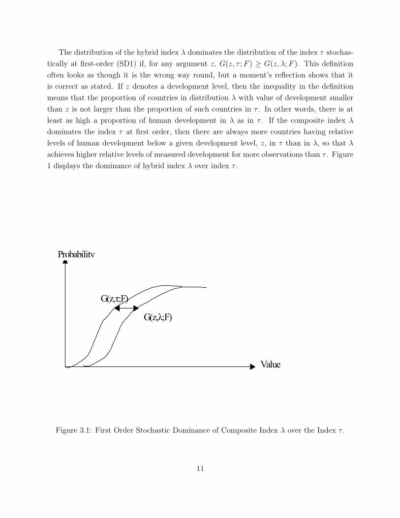
The distribution of the hybrid index λ dominates the distribution of the index τ stochas-

tically at first-order (SD1) if, for any argument z, G(z, τ ; F ) ≥ G(z, λ; F ). This definition

often looks as though it is the wrong way round, but a moment’s reflection shows that it

is correct as stated. If z denotes a development level, then the inequality in the definition

means that the proportion of countries in distribution λ with value of development smaller

than z is not larger than the proportion of such countries in τ . In other words, there is at

least as high a proportion of human development in λ as in τ . If the composite index λ

dominates the index τ at first order, then there are always more countries having relative

levels of human development below a given development level, z, in τ than in λ, so that λ

achieves higher relative levels of measured development for more observations than τ . Figure

1 displays the dominance of hybrid index λ over index τ .

G(z,τ;F)

G(z,λ;F)

Value

Probability

Figure 3.1: First Order Stochastic Dominance of Composite Index λ over the Index τ .

11

The objective function that we use is the following:

Maxz,λ

[G(z, τ ; F )−G(z, λ; F )]

The above maximization results in the best-case scenario (most optimistic) hybrid index λ

constructed from the set of components in the sense that it reaches the highest level of mea-

sured human development for a given probability, implying that the number of observations

having a relative development level above a given argument z is maximized.

It is worth mentioning that SD is considerably more general than mean-variance analysis

which only looks at the first two moments of the two distributions under comparison. The

latter only looks into a dominant relation with a higher mean and lower variance, whereas

the former considers all possible moments. Only in the case where we compare two normal

distributions does SD reduce to mean-variance analysis. This is also true for PCA which is

based on the consideration of the second moment alone after standardizing for a common

mean. However, the assumption of normality for each component is difficult to support

empirically. In contrast, SD analysis takes into account the whole distribution, not only

the mean and the variance. Hence, we could expect significant differences between the SD

efficient index and the mean-variance efficient index when more realistic assumptions are

made concerning the distributions of the different components. SD is attractive because it

is effectively nonparametric as no explicit specification of a utility function or probability

distribution functional form is required. In addition, the entire probability density function

is taken into account rather than a finite number of moments so it can be considered less

restrictive and more robust.

When studying welfare measures, certain criteria need to be satisfied. The SD1 criterion

corresponds to all types of utility functions as long as they are non-decreasing in development

levels. SD1 only relies on the fact that people are rational in the sense that they prefer more

rather than less development (also known as the monotonicity axiom). In other words, a

sensible aggregate welfare measure should be increasing in any indicator which is increasing in

a social ‘good’, and decreasing in any indicator which represents a social ‘bad’. Accordingly,

for aggregate welfare indices containing only social ‘good’ indicators, one hybrid outcome

as expressed by the index λ should be ranked higher than that of another hybrid outcome

expressed by the index τ if at least one country is better off in λ than in τ , and no one is

worse off. So, SD1 of τ by λ means that λ corresponds to a higher measured relative welfare

than τ .

When there is no hybrid index λ that dominates the given index τ at first-order, we move

12

to the SD2 criterion. The objective function that we use is the following:

Maxz,λ

∫ z

−∞G(u, τ ; F )du−

∫ z

−∞G(u, λ; F )du

This maximization results in the most optimistic hybrid index λ constructed from the set

of components in the sense that it also gives the greatest value of human development for a

given probability.

We can further define for z ∈ R:

J1(z, λ; F ) := G(z, λ; F ),

J2(z, λ; F ) :=

∫ z

−∞G(u, λ; F )du =

∫ z

−∞J1(u, λ; F )du,

J3(z, λ; F ) :=

∫ z

−∞

∫ u

−∞G(v, λ; F )dvdu =

∫ z

−∞J2(u, λ; F )du,

and so on.

From Davidson and Duclos (2000) Equation (2), we know that

Jj(z, λ; F ) =

∫ z

−∞

1

(j − 1)!(z − u)j−1dG(u, λ, F ),

which can be rewritten as

Jj(z, λ; F ) =

∫Rn

1

(j − 1)!(z − λ′u)j−1Iλ′u ≤ zdF (u).

The general hypotheses for testing SD efficiency of order j of τ , hereafter SDJ , can be

written compactly as:

Hj0 :Jj(z, τ ; F ) ≤ Jj(z, λ; F )for all z ∈ R and for all λ ∈ L,

Hj1 :Jj(z, τ ; F ) > Jj(z, λ; F )for some z ∈ R or for some λ ∈ L.

Under the null Hypothesis Hj0 there is no hybrid index λ constructed from the set of compo-

nents that dominates the index τ at order j. In this case, the function Jj(z, τ ; F ) is always

lower than the function Jj(z, λ; F ) for all possible hybrid indices λ for any argument z.

Under the alternative hypothesis Hj1 , we can construct a hybrid index λ that for some argu-

ments z, the function Jj(z, τ ; F ) is greater than the function Jj(z, λ; F ). Thus, the index τ

is SD1 inefficient if and only if some other hybrid index λ dominates it. Alternatively, index

τ is SD1 efficient if and only if there is no hybrid index λ that dominates it.

13

In particular we obtain SD1 and SD2 when j = 1 and j = 2, respectively. The hypothesis

for testing SD of order j of the distribution of index τ over the distribution of index λ takes

analogous forms, but for a given λ instead of several of them.

In what follows we will consider how to test for SD of a single composite index over time.

We will then proceed to obtain the test statistic for testing for SDE of the equally-weighted

HDI.

3.2 Tests for SD of a single composite index over time

In subsection 3.3 below we will present the test statistic for the SD efficiency of the HDI.

Before we do that, our objective is to examine the stochastic dominance of the HDI over

a twenty-five year period and determine which factors drive its improvement over time. In

this case we have a pair-wise comparison of a given index over two points in time, such as

the equally-weighted HDI, τ , in year 1975 and in year 1980. We define G(z, τ ; F ) the cdf of

the index at point z given by G(z, τ ; F ) :=

∫R

Iτ ′u ≤ zdF (u).

We focus on a situation in which we have (possibly) dependent samples of indices from two

populations (such as a group of countries at two different points in time) that have associated

cumulative distribution functions (cdf ′s) given by G and F , and the functions Jj(z, τ ; G)

and Jj(z, τ ; F ). In this context, SD1 of G over F corresponds to J1(z, τ ; G) ≤ J1(z, τ ; F )

or G(z, τ ; G) ≤ G(z, τ ; F ) for all z. When this occurs social welfare in the population

summarized by G is at least as large as that in the F population, when U is any increasing

monotonic function of z − i.e., U ′(z) ≥ 0. The cdf of F is always at least as large as that of

G, i.e., distribution F always has more mass in the lower part of distribution.

How is this related to HDI dominance? Suppose we have n countries in total. If the cdf

of HDI in 1975, F (z), is always at least as large as that of the cdf in 1985, G(z) at any point,

then the proportion of countries below a particular index level for the year 1975 is higher

than that of 1985. Therefore, the 1985 HDI stochastically dominates its 1975 counterpart

in the first-order. When the two cdf curves intersect, then the ranking is ambiguous. In

this situation we cannot state whether one distribution first-order dominates the other. This

leads to an ambiguous situation which makes it necessary to use higher-order SD analysis.

SD2 of G over F corresponds to J2(z, τ ; G) ≤ J2(z, τ ; F ) for all z and the social welfare

in the population summarized by G is at least as large as that in the F population, for

any utility function U that is monotonically increasing and concave, that is U ′(z) ≥ 0

and U ′′(z) ≤ 0. Second-order stochastic dominance is verified, not by comparing the cdf ′s

themselves, but comparing the integrals below them. We examine the area below the F (z)

and G(z) curves. Given lower and upper boundary levels, we determine the area beneath the

14

curves and, if the area beneath the F (z) distribution is larger than the one of G(z), then in

this case G(z) stochastically dominates F (z) in the second-order sense. Since we look at the

area under the distributions, second-order dominance implies simply an overall improvement

and not a point-wise dominance over all the points of the support of one distribution over

another.

There is no guarantee that SD2 will hold, so one may want to look for third-order dom-

inance. Third-order stochastic dominance (SD3) of G over F corresponds to J3(z, τ ; G) ≤J3(z, τ ; F ) for all z and the social welfare in the population summarized by G is at least

as large as that in the F population for any utility function U that satisfies U ′(z) ≥ 0,

U ′′(z) ≤ 0, and U ′′′(z) ≥ 0. This is the case of third-order stochastic dominance and it is

equivalent to imposing the condition that it places a higher weight on lower levels of indices.

The general hypotheses for testing SD of the index over time of order j can be written

compactly as:

Hj0 : Jj(z, τ ; G) ≤ Jj(z, τ ; F ) for all z ∈ [0, z] ,

Hj1 : Jj(z, τ ; G) > Jj(z, τ ; F ) for some z ∈ [0, z] .

Stochastic dominance of any order of G over F implies that G is no larger than F at

any point. In this case there is an improvement of the index over time. Thus, if the HDI in

1980 dominates the HDI in 1975, then there is an improvement in the measured development

level of each country over time. The alternative hypothesis is the converse of the null and

implies that there is at least some index value at which G (or its integral) is strictly larger

than F (or its integral). In other words SD fails at some point for G over F . In this case,

there can be improvements in development levels for some countries and no improvement or

even deterioration of development levels for some other countries over time. Hence, there is

no general improvement for all countries simultaneously over time.

3.2.1 Test Statistics

We consider two time-dependent samples from two distributions (e.g., for HDI in 1975 and

1980). In order to allow for different sample sizes we need to make assumptions about the

way in which sample sizes grow.

Assumption 1:

(i) XiNi=1 and YiM

i=1are independent random samples from distributions with

CDF ′s F and G respectively;

(ii) the sampling scheme is such that as N, M −→∞, NN+M

= φ where 0 < φ < 1.

Assumption1(i) deals with the sampling scheme and would be satisfied if one has samples

15

of indices from different segments of a population or separate samples across time. Assump-

tion1(ii) implies that the ratio of the sample sizes is finite and bounded away from zero.

The empirical distributions used to construct the tests are respectively,

FN(z) = 1N

N∑i=1

I(Xi ≤ z), GM(z) = 1M

M∑i=1

I(Yi ≤ z).

The test statistics for testing the hypotheses can be written compactly as follows:

Sj =(

NMN+M

)1/2sup

z(ζj(z; GM)− (ζj(z; FN)).

Since ζj is a linear operator, then

ζj(z; FN) =1

N

N∑i=1

ζj(z; IXi) =

1

N

N∑i=1

1

(j − 1)!I(Xi ≤ z)(z −Xi)

j−1 (3.1)

where IXidenotes the indicator function I(Xi ≤ x) (Davidson and Duclos 2000).

The asymptotic properties of the tests are gathered in appendix A. We consider tests

based on the decision rule:

reject Hj0 if Sj > cj

where cj are suitably chosen critical values to be obtained by simulation methods.

In order to make the result operational, we need to find an appropriate critical value cj to

satisfy P (SF

j > cj) ≡ α or P (SG,F

j > cj) ≡ α (some desired probability level such as 0.05 or

0.01). Since the distribution of the test statistic depends on the underlying distribution, we

rely on bootstrap methods to simulate the p-values. We discuss these methods in appendix

D1.

3.3 Tests of the SD efficiency of the HDI

In the previous section, we discussed stochastic dominance tests of HDI and each separate

sub-index over time by considering a pair-wise comparison of a given index over two points

in time. In this section, we derive statistics to test for SD efficiency of the official HDI,

τ , i.e., equal weights given to each sub-index, with respect to all possible combinations of

weighting schemes (λ) constructed from the given set of components.

Jj(z, λ; F ) =1

T

T∑t=1

1

(j − 1)!(z − λ′Y t)

j−1Iλ′Y t ≤ z,

16

This can be rewritten more compactly for j ≥ 2 as:

Jj(z, λ; F ) =1

T

T∑t=1

1

(j − 1)!(z − λ′Y t)

j−1+ .

3.3.1 Test Statistics

We consider the weighted Kolmogorov-Smirnov type test statistic

S :=√

T1

Tsupz,λ

[G(z, τ ; F )−G(z, λ; F )

],

and a test based on the decision rule:

reject Hj0 if Sj > cj ,

where cj is some critical value (see ST, section 2 for the derivation of the test). The asymp-

totic properties of the test statistic are collected in appendix B. In order to make the result

operational, we need to find an appropriate critical value cj. Since the distribution of the

test statistic depends on the underlying distribution, we rely on a block bootstrap method

to simulate p-values. We discuss how to obtain simulated p-values for dependent data using

bootstrapping methods in appendix D2.

4 Mathematical formulation of the test statistics for

SD1

Testing for SD1 is based on the following test statistic S1, derived using mixed integer

programming formulations. The full formulation of the testing problem is given below:

maxz,λ

S1 =√

T1

T

T∑t=1

(Lt −Wt) (4.1a)

s.t.M(Lt − 1) ≤ z − τ ′Y t ≤ MLt, ∀ t (4.1b)

M(Wt − 1) ≤ z − λ′Y t ≤ MWt, ∀ t (4.1c)

e′λ = 1, (4.1d)

λ ≥ 0, (4.1e)

Wt ∈ 0, 1, Lt ∈ 0, 1, ∀ t (4.1f)

17

with M being a large constant.

The model is a mixed integer program maximizing the distance between the sum over

all scenarios of two binary variables,1

T

T∑t=1

Lt and1

T

T∑t=1

Wt which represent G(z, τ ; F ) and

G(z, λ; F ), respectively (the empirical cdf of τ and λ at point z). According to inequalities

(4.1b), Lt equals 1 for each scenario t ∈ T for which z ≥ τ ′Y t, and 0 otherwise. Analogously,

inequalities (4.1c) ensure that Wt equals 1 for each scenario for which z ≥ λ′Y t. Equation

(4.1d) defines the sum of all index weights to be unity, while inequality (4.1e) disallows

negative weights. This formulation allows for a test of the dominance of the equally-weighted

HDI, τ , over any potential linear combination λ of the components. When some of the

variables are binary, corresponding to mixed integer programming, the problem becomes

NP-complete (non-polynomial, i.e., formally intractable).

We can see that there is a set of at most T values, say R = r1, r2, ..., rT, containing

the optimal value of the variable z. A direct consequence is that we can solve the original

problem by solving the smaller problems P (r), r ∈ R, in which z is fixed to r. Then we take

the value for z that yields the best total result. The advantage is that the optimal values of

the Lt variables are known in P (r).

The reduced form of the problem is as follows (see appendix E1 for the derivation of this

formulation and details on its practical implementation)

minT∑

t=1

Wt

s.t.λ′Y t ≥ r − (r −Mt)Wt, ∀t ∈ T

e′λ = 1,

λ ≥ 0,

Wt ∈ 0, 1, ∀t ∈ T. (4.2a)

A similar procedure is used in the formulation of the test statistic for SD2. The exact

formulation for testing for SD2 is presented in appendix E2.

We derived statistics to test for SD efficiency of the official HDI (i.e., each sub-index being

equally weighted) with respect to all possible combinations of weighting schemes constructed

from the set of components. In the next section, before moving to the empirical analysis

of HDI, we present some simulation experiments to evaluate the importance of different

distributional component characteristics in the derivation of best-case scenario optimistic

18

weights.

5 Simulation Experiments

We present simulation results for three different experiments. In each case we have three dif-

ferent components (as in the case of HDI) all normally distributed that are used to construct

the equally-weighted composite index using 500 observations. The results are reported in

Table 1.

In the first experiment, we simulate three components which are normally distributed

with each component having the same mean, 0.5, and same variance, 0.1 and we construct an

equally-weighted composite index from these simulated components. The results of the first

panel of Table 1 show that there is no case that dominates the equally-weighted composite

index and there are 164 cases which have the same efficiency as the equally-weighted index.

In the second case, we simulate three normally distributed components with the same

mean, 0.5. However we allow for different component variances, 0.15, 0.1 and 0.05 respec-

tively, something that would enable us to see directly the effect of variability on the construc-

tion of the composite index. The results in the second panel of Table 1 show that there are

203 composite indices for a given “z” point that dominate the equally-weighted composite

index and it is clear that the least variable component has the greatest impact. In that

case, the least variable component’s weight (the third component) from these 203 dominant

indices is on average 0.6589. On the other hand the second and third least variable com-

ponents with respective variances 0.1 and 0.15 have weights 0.2589 and 0.0822 respectively.

The above simulation results suggest that using the fixed equal weighting scheme will result

in an index that is dominated by many other potential hybrids with different weights. One

can see that when the means of each component are the same, the least variable component

has the greatest impact on the construction of the most optimistic index.

In the third experiment, we allow the three components to have different mean values,

0.55, 0.5 and 0.45 respectively. Given these mean values, we allow for different possible

variance (standard deviation) combinations, where each component takes a different standard

deviation value in each case from a set of 0.05, 0.1, 0.15. The results of the third panel

show that other things being equal, the component with the highest mean has more impact

and gets more weight (as in the 1st row where the first component gets a weight of 0.77).

However, the weight drops if the component with the highest mean has also the highest

variance, as seen in the second row where the average weight falls to 0.70 from 0.77. There

is an offsetting effect as a higher mean implies a higher weight, whereas the opposite is true

19

for a higher variance (higher variability).

Overall, we find that when all components have the same mean and the same standard

deviation, the equally-weighted composite index is efficient and there is no hybrid index

that dominates it. On the other hand, when each component has the same mean and

different standard deviations, then the least variable component has the greatest impact

on the construction of the most optimistic index. When each component has a different

mean and the same standard deviation, then the component with the higher mean has

the greatest impact. When both mean and standard deviations vary, then the component

with the highest mean and the lowest variability relative to the other components has the

greatest impact on the construction of the best-case scenario index. There is a trade off

between mean and variance and in the case where one component has the highest mean and

highest standard deviation and the other component has the second highest mean but is less

variable, then both components would have almost an equal impact on the construction of

the most optimistic index.

5.1 Data augmentation with heterogeneous new entrants

In order to check the robustness of the simulation results presented in Table 1, we will

investigate whether these will change when we add countries (observations) with different

characteristics. Taking as given the means and standard deviations of the existing data

series (the three components have mean values of 0.55, 0.5 and 0.45 respectively and the

same standard deviation 0.1) we allow for 100 more observations to be added to the existing

data. The results are presented in the fourth panel of Table 1.

In the first experiment, the 100 new entrants of the second and third components have

the same mean values of 0.5 and 0.45 respectively and the same standard deviations of 0.1

as before. However, the statistical characteristics of the first component are different than

before for these additional 100 new entrants, with a mean of 0.6, and different variance

(standard deviation) combinations, 0.05, 0.1, 0.15. We observe that the weights do not

vary significantly when these new observations (new countries) with different characteristics

enter into the simulation experiment. At the first row, we observe that the changes of weights

to each component are -0.0074, 0.0064 and 0.0010 respectively. As the overall mean of the

first component increases, its weight increases slightly without changing much the nature of

the previous results. We observe that the largest change in the components’ weights is only

about 2%.

In the second experiment, the 100 new entrants of the first and third components have

the same mean values of 0.55 and 0.45 respectively and the same standard deviations 0.1, but

20

the statistical characteristics of the second component are different from before for the 100

new entrants, with a mean of 0.6 and different variance (standard deviation) combinations,

0.05, 0.1, 0.15. Again, the weights do not vary significantly when new countries with

different characteristics enter into the simulation experiment. Since the mean of the second

component is now greater, its weight now slightly increases. Even in this case the largest

change in the components’ weights is only about 3%.

In the third experiment, the 100 new entrants of the first and second components have

the same mean values of 0.55 and 0.5 respectively, and the same standard deviations 0.1,

but the statistical characteristics of the third component are different from before for the

100 new entrants, with a mean of 0.6 and a standard deviation that takes values from the

set 0.05, 0.1, 0.15. Since the mean of the third component is now greater, there is a small

increase in its weight. In this case also the largest change in the weights is only about 2.5%.

Overall, we observe that the entrance of new (observations) countries with different sta-

tistical characteristics will result in a 2% to 3% change in the relative weights attached to the

individual components. We found that even though the number of observations increased by

20% with 100 new entrants, the change in the resulting weighting scheme is minor. Since we

have a total of 1264 observations in the existing HDI data set, we anticipate that any new

additions to the HDI data set that may occur in one of the following 5-year periods will be

of a smaller magnitude than that, with expected weight changes being less than 2%.11

In the above experiments we observe the role of the mean in arriving at these weights.

The SD approach maximizes the distributional distance between the given (equally-weighted)

index and any possible alternative. In comparing distributions, we know that the mean plays

the key role, followed by variability. The mean indicates the achievement level offered by

each component, while the standard deviation shows the variability of the achievement. The

most optimistic index obtained from the stochastic dominance approach is the one that

measures the greatest achievement over time, the greatest measured development level, and

at the same time exhibits discernibly the most stable performance.

In this section, we examined the importance of component statistics to derive the most

optimistic weights. In the following section, we will proceed with the application of SD

analysis to the HDI data. We will first present the descriptive statistics of HDI and its

components followed by the SD analysis of each component over time and the derivation of

the most optimistic weights.

11We also repeated without reporting the same procedure by adding 50 and 25 new entriesrespectively (10% and 5% of the existing data set). In all cases, the changes in the relative weightingscheme are minor, less than 2% for each component.

21

6 Empirical Analysis of SD efficiency of HDI

6.1 Data and Descriptive Statistics

We use the United Nations Development Program’s HDI and its components - life expectancy,

education and GDP indices for the period 1975 to 2000 in 5-year increments. Each index

ranges between 0 and 1 (from lowest to highest well being). The HDI represents the simple

arithmetic average of the three individual indices.

The definition of the life expectancy index (LE) is given by LE = LE−2585−25

. The life ex-

pectancy raw data series has an upper bound of 85 and a lower bound of 25 years. The

value of a country’s life expectancy index is obtained by the country’s life expectancy in

years minus 25 divided by 60, for a number that would lie between 0 and 1. The education

index (E) is defined as E= 23(adult literacy index) + 1

3(gross enrollment index). This index

is constructed so that a 2/3 weight is given to literacy (percentage of the population that is

considered literate) and a 1/3 weight is given to gross school enrollment as a percentage of

the eligible school age population and it is bounded between 0 and 1. Finally, the GDP per

capita index is defined as, GDP Index= log (GDP per capita) - log (100)log (40000)-log (100)

. It is created in a similar

manner as LE, where the upper bound for the raw GDP per capita series is 40000 and the

lower bound is 100 US dollars per capita. The values taken by the index lie in the (0,1)

range. Each separate index is then equally weighted to create the HDI.12

Table 2 presents the descriptive statistics for HDI and the individual component indices

over time. It is evident that HDI improved over time, as did LE and E, whereas the GDP

per capita index remained almost unchanged between 1980 and 1995, while it fell in the

period from 1980 to 1985. We see that E increased significantly over this time period, while

LE remained steady after 1990. This is mainly because of the fall in life expectancy in

Africa. It appears that education has the largest mean among the components, whereas all

three have similar standard deviations. Given the simulation results of the previous section,

the descriptive statistics suggest that education would be the dominant component of the

best-case scenario index based on SDE testing, something that we will verify below.13 In

12Starting from 2010, the UNDP made adjustments to how the HDI is constructed. Not onlythe definitions of some components but also the upper and lower bounds of the raw componentshave changed. The component indices of HDI after the year 2010 are calculated as: Income index(II): ln(GNI per capita) - ln(163)

ln(108211)-ln(163) . Education index (EI)=√

MY S·EY S0.951 where mean years of schooling (MYS)

index=MY S−013.2−0 and Expected years of schooling (EYS) index=EY S−0

20.6−0 . Life expectancy index (LEI):LE−2083.2−20 . Finally, HDI is obtained by the geometric mean of the those three indices: 3

√II · EI · LEI.

13Even if we standardize using the means and variances for each index, each index’s empiricaldistribution will remain the same. In that case, for example, the education index will continue tobe negatively skewed and most of the outcomes will be greater than the standardized zero mean.

22

the next section we will examine the SD dominance results for these indices separately to

establish the dominant component that drives the HDI improvements over time.

6.2 Results for SD tests

We will discuss the results of Kolmogorov-Smirnov tests for HDI and its components sep-

arately. Table 3 presents the results for SD1 and SD2 over the period under investigation

based on bootstrap methods from BD for stochastic dominance with dependent data. For

completeness, in Table 4, we also apply the Linton et al. (2005) subsampling approach to HDI

and its components to compare the findings with the BD sampling approach. We first test

whether the HDI in 1980 dominates the HDI in 1975, and separately we test whether each

individual component (e.g., education) in 1980 dominates this component in 1975 in order to

establish whether over time improvements have occurred and in addition, which component

is mainly responsible for such improvements. The vertical column of Table 3 represents the

years from 1980 to 2000 that are tested for stochastic dominance against years from 1975 to

1995. Percentage levels in the table represent the significance level of stochastic dominance

(e.g., in the first panel of Table 3: 1980 year HDI stochastically dominates the 1975 year in

the second-order sense at the 10 percent level). N/A means that there is no dominance at

that order.14

The results in Table 3 suggest that there is no improvement for any index using a 5 year

testing horizon. In all such cases SD1 is rejected. However, apart from the GDP index, all

other indices display significant improvements using a 10 year horizon. In almost all 10 year

or greater periods, there is dominance at first-order at the 1% significant level, for education

and life expectancy, although not as strong for the latter as for the former. The exception

is the GDP index, where as seen in the fourth panel of Table 3, there are no discernible

significant improvements over the whole period.

It becomes apparent that the improvements in the HDI over time are driven by the

improvement in education and life expectancy. However, the improvement in education

index occurs even in 5-year periods in a second-order sense, something that implies that

education may be improving more rapidly over shorter time periods.

We proceed to use the Linton et al. (2005) subsampling approach to HDI and its compo-

nents in order to compare its findings with those of the BD bootstrapping approach presented

in Table 3. The same number of countries is used to test if there are first and second-order

Therefore, even if we standardize each index, we will get exactly the same results as before.14We first test for SD1: if there is dominance at first-order, then there will be dominance at any

other greater order. If not, then we continue for SD2.

23

of dominance over time for each component of HDI. Table 4 presents the results for SD1

and SD2 for HDI and its components respectively. The null hypothesis is that the respective

index in the following years dominates the index of the previous years and we report p-values

for SD1 and SD2. We observe that in general, the null hypothesis is not rejected, suggesting

the presence of an overall improvement over time for all indices. The only exception is that

we reject the null hypothesis that the 1990 life expectancy dominates 1985 life expectancy

at any order. The same is true for the period 1990 to 2000.

There are some differences between the BD and the Linton et al. (2005) results. The

most striking one is that the GDP per capita index has shown an improvement over time

when we use the latter approach as opposed to the former. There are two main reasons

for this. The first one is that for the BD approach we allow for an unbalanced panel, as a

different number of countries can be examined over time. This is not the case for the Linton

et al. (2005) approach that requires a balanced, and as a result a more homogeneous, panel

for its analysis. The second reason is that the null hypothesis in the BD approach excludes

equality from dominance, whereas it is included in the null hypothesis of Linton et al. (2005).

In that case, there may be under-rejection of dominance over time as there could be many

equal outcomes that would favour dominance.

In this section, we applied SD analysis over time to each component sub-index in order

to establish the dominant one responsible for the overall improvement of HDI over time.

The SD tests were conducted using pair-wise comparisons for each separate sub-index over

time, without allowing for differential weights for each component. In the next section, we

will allow for full diversification of weights to test whether assigning equal weights to each

sub-index leads to the most optimistic view or whether alternative weighting schemes imply

higher relative development levels and less variability across countries and over time.

6.3 SDE Results for HDI

We continue with our findings of the test for SD1 efficiency of the HDI. We found that

the equally-weighted HDI does not offer the best-case scenario. We can construct many

other hybrid composites λ consisting of the three components of the HDI (life expectancy,

educational attainment, and GDP per capita) that stochastically dominate the equally-

weighted HDI, τ , in the first-order sense (e.g., for which G(z, τ ; F ) > G(z, λ; F )). There are

293 different such composite λ’s. Table 5 summarizes the results. This table presents the

average weights of the 293 hybrid composites that dominate the standard HDI. It is clear

that education has the greatest impact with a 71.17% (0.7117) weight. On the other hand,

life expectancy and GDP per capita take weights of 12.38% (0.1238) and 16.45% (0.1645)

24

respectively. The inefficiency of the official HDI indicates that the equal weighting scheme

achieves lower levels of measured development as there are alternative weighting schemes

that assign a higher measured development level to each country. SDE analysis allows us to

derive the most optimistic weighting scheme where more countries achieve higher measured

development levels and less variability both cross-sectionally and over time. Furthermore, the

weights derived from SDE analysis can be thought of as explicit weights that lead to the most

optimistic development scenario, where the emphasis is placed on educational improvements.

The empirical findings confirm the simulation results of the previous section. Education is

the dominant constituent component of the most optimistic index as it dominates in terms

of mean the other two (even though in terms of variance all three components are quite

similar). In this case, education is the key factor that leads to the best-case development

scenario, where higher and more stable relative measured levels of development are achieved

cross-sectionally and over time.

We also conducted some additional robustness analysis. We allowed for the possibility

that the importance of education in the construction of the most optimistic scenario of the

HDI changes as we move to a more qualitative measure of education. Education attainment

in the HDI consists of a country’s adult literacy rate and gross enrollment rate which repre-

sent quantitative measures of a given country’s educational level. We repeated the analysis

using data that capture the quality of educational attainment only as well a combination of

both quality and quantity. As measures of quality of education we considered data from the

Trends in International Mathematics and Science Study (TIMSS), from the Programme for

International Student Assessment (PISA) and from the Progress in International Reading

Literacy Study (PIRLS). However, the data set on the quality of education is limited, since

these data were first collected only in the mid-1990s. The Trends in International Mathe-

matics and Science Study (TIMSS) conducted tests in mathematics and science to test the

achievements for fourth- and eighth-grade students for each of the participating countries

in 1995, 1999, 2003, 2007 and 2011. The Programme for International Student Assessment

(PISA) implemented tests for science, mathematics and reading achievements of students

in 2000, 2003, 2006 and 2009. Lastly, Progress in International Reading Literacy Study

(PIRLS) had a literacy assessment in 2001, 2006 and 2011. Since we have data for HDI until

2003, we have coverage by the TIMSS for the three years 1995, 1999 and 2003, the PIRLS

assessment for year 2001 and the PISA assessment for 2000. Therefore, we have quality of

education data for the years 1995, 1999, 2000, 2001 and 2003 with a total of 160 observations.

The number of countries covered in each of these years are 38, 29, 25, 29 and 39 respectively.

Each country’s science, mathematics and reading achievement is scaled to lie between zero

25

and one.15

We test three different cases and we combine the results. In the first case we have 160

observations using data that represent the quantitative aspect of education (as in the original

HDI), life expectancy and the GDP index to test whether the standard HDI offers the best-

case scenario. In the second case, we replace the education index by the quality of education

index and obtain an adjusted HDI by giving equal weights to each index (i.e., life expectancy

and the GDP index remain the same, but the education index is replaced by the quality of

education index). We then test whether this HDI offers the most optimistic view. Finally,

in the third case, we combine the quality and quantity of education indices by giving equal

weight to each component. We obtain an equally-weighted HDI for this case and we test

whether it is the best-case scenario with respect to SD1 efficiency. Overall, regardless of

the way education is measured, it has the greatest impact on the construction of the most

optimistic view of HDI. The impact of education is the lowest (80.04%) when the quality

of education index is used, while it is highest (86.29%) when the quantity of education is

used.16

Next, we will present country rankings for the years 1995, 2000 and 2006 using the most

optimistic view of HDI that resulted from the stochastic dominance tests (e.g., with weights

71.17% for education, 12.38% for life expectancy and 16.45% for GDP per capita) and the

equally-weighted standard HDI.17 The first panel of Table 6 presents the rankings of the top

twenty countries using both the best-case scenario and the standard HDI for years 1995, 2000

and 2006. For example for 2006, we observe that Sweden, Japan, and Switzerland moved

out of the top 10 group under the equally-weighted HDI and they were replaced by Finland,

Denmark and New Zealand in the new ranking. Iceland, Ireland and Netherlands remained

in the top ten group of countries moving however to a lower ranking position. Australia

moved to a higher ranking, Norway remained at the second position, while Canada now

moved to the highest spot.

The second panel of Table 6 reports the twenty countries that moved to a higher ranking

position in years 1995, 2000 and 2006 under the most optimistic view of HDI relative to the

standard HDI (e.g., for 2006, Guyana ranked at the 110th position under the standard HDI

15The scaling is done using the achievement of a country at a given year divided by the maximumachievement for that given year.

16The average weights of education are now higher, since the data set for the quality of educationis limited, with 160 observations confined only to the set of developed and more homogeneouscountries. The results are available upon request from the authors.

17It is worth noting that the new ranking is highly correlated with the original ranking. TheSpearman correlation between the old and new ranking is 0.95. This is to be expected since all theoriginal components are highly correlated and the composite indices are constructed as weightedaverages of these components.

26

moved to the 73rd position under the best-case scenario of the HDI, an improvement in its

ranking of 37 positions). The main reason that these countries moved to a higher ranking

under the most optimistic view of the HDI is that most of them, such as Ukraine, Kazakhstan,

Kyrgyzstan, Belarus, Turkmenistan and Russia were part of the Soviet Union that had a

good educational system, even though GDP per capita was relatively low. Furthermore, the

large upward ranking changes occur because these countries are the ones experiencing bad

outcomes not only in their GDP per capita but also in life expectancy. In that case, equally

weighting each index would understate these countries’ achievement at the educational level.

In the third panel of Table 6 we report the twenty countries that moved to a lower ranking

position under the most optimistic view of the HDI relative to the standard HDI in years

1995, 2000 and 2006. For example for 2006, Oman ranked at the 53rd position with the

equally-weighted index moved to be 101st under the best-case scenario optimistic index, a

deterioration of 48 positions. The main reason that these countries moved to a lower ranking

is that they have relatively higher GDP per capita, as most of them are resource-dependent

economies (oil producers), with relatively fewer resources allocated to education. As a result,

their educational achievements lag behind those of other countries. We should note that a

resource-dependent country could still invest in education if the country has a social structure

that allows its citizens to access resources equally and/or redistribute its achievement in one

attribute (i.e., standard of living) through fostering other dimensions (i.e., life expectancy

and education). Therefore, we further analyze the raw components of the education index

for those countries that moved to a lower ranking. One of the main factors behind the

weakness of their educational system appears to be high gender inequality (i.e., low female

participation in the educational system).18

We proceed to examine the improvement in the relative levels of human development

when the most optimistic weighting scheme is used. In this context, we address the following

question: “If we weight the components to arrive at the most optimistic view of human

development, across countries and in earlier time periods, then to what extent has there been

18In 1995, 16 out of 20 countries experienced a high gender inequality in adult literacy rates. Forexample, percentages of literacy rates are 46% and 71% for female and male respectively in Oman.Similarly, for Saudi Arabia (50.3% and 71.5%), for Kuwait (74.9% and 82.2%), for Algeria (49.1%and 73.9%), for Turkey (72.4% and 91.7%), for Iran (59.3% and 77.7%), for Tunisia (54.6% and78.6%), for Syria (55.8% and 85.7%), for Malaysia (78.1% and 89.1%), for Singapore (86.3% and95.9%), for Hong Kong (88.2% and 96%), for Mauritius (78.8% and 87.1%), for Egypt (38.8%and 63.3%), for Morocco (31% and 56.6%), for Guatemala (57.2% and 72.8%) and for Botswana(59.9% and 80.5%) respectively for female and male literacy rates. It is also worth mentioning thatfor Luxembourg, Singapore and Hong Kong, even though literacy rates are very high, their grossenrollment ratios are around 60-70% as the majority of the population from those countries leaveto pursue higher education in other countries.

27

a general improvement over time under this best-case scenario?” In order to examine the

improvement in human development over time, we compare the percentages of countries that

fall into different human development groups (i.e., low, medium, high and very high human

development groups) using the official HDI with that using the optimistic weighting scheme

for the years 1995, 2000 and 2006. The UNDP’s Human Development Report separates

countries into low, medium, high and very high human development groups where each group

consist of countries that have HDI values less than 0.5, between 0.5 and 0.799, between 0.8

and 0.899, and above 0.9 respectively.

The first panel of the Table 7 presents the percentage of countries in each human devel-

opment group with the official HDI in 1995, 2000 and 2006, whereas the second panel of the

Table 7 offers the same information for the best-case scenario case. Over time, there would

always have been a lower percentage of countries in the low and medium human development

groups and a higher percentage of countries in the high and very high human development

groups with the most optimistic case than the official HDI. With both the official HDI and

the most optimistic scenario, the percentage of countries in the low development group de-

creased over time. However, the change in the percentage of countries that fall into the

medium, high and very high human development groups does not follow a particular pat-

tern over time with the official HDI. From 1995 to 2000, the percentage of countries in the

medium development level group increased (from 38% to 49%), whereas the percentages of

countries in both the high and very high development groups decreased (from 22% to 19%

and 15% to 12% respectively) with the official HDI. From 2000 to 2006, the percentage of

countries in the medium development level group decreased (from 49% to 44%) and both

the percentages of countries in the high and very high development groups increased (from

19% to 23% and 12% to 18% respectively) with the official HDI. On the other hand, with

the optimistic scenario case, there is a distinct improvement over time. Both the percentages

of countries in the low and medium human development groups decreased over time, while

the percentages of countries in both the high and very high human development groups

increased. For the 1995 to 2006 period, a percentage of countries moved from the low to

the medium development group but there have been even more countries that moved from

the medium to the high and very high human development groups. In 2006, almost 60%

of the countries were categorized in the high and very high development groups with the

optimistic scenario case, while there were around 40% of the countries in the high and very

high development groups with the official HDI.

Overall, we observe that when we change the weighting scheme in the construction of

HDI, the ranking of countries will change. Although it has been suggested that weighting

28

each index differently should not change the ranking when the correlation is high among the

constituent indices (as is here the case), the SD approach demonstrates that weighting each

index differently does have an impact on outcomes.19

7 Conclusion

In this paper we employ consistent SD tests to examine whether there has been a general

improvement in the official HDI and its components over time. The results suggest that there

is no general improvement for any index using a five-year testing horizon (subperiods within

1975 to 2000). However, apart from the GDP index, all other indices display significant

improvements using a ten-year horizon. In almost all ten year or greater periods, there is a

general improvement in education and life expectancy, although not as strong for the latter

as for the former. Moreover, there is no general improvement in the life expectancy index

between the period 1990 and 2000. For the GDP index, there are no discernible significant

general improvements over the whole period. In other words, the improvement in the official

HDI over-time is mainly driven by improvements in the education index, the fast-responding

indicator to its targets. This indicator has shown improvements for all countries within the

ten-year horizon periods, whereas life expectancy and the GDP index are the slow-moving

indicators holding back the overall improvement in the official HDI.

Moreover, we present tests for SDE of any order for time-dependent data. We apply

tests for SDE of a given index with respect to all possible indices constructed from a set of

individual components. We proceed to test whether SDE justifies the use of the standard

equally-weighted HDI, when compared with any other index constructed with alternative

weights for the three constituent components: education, life expectancy and GDP per

capita. SDE analysis results in the most optimistic weighting scheme where more countries

display higher measured relative development levels and less variability both cross-sectionally

and over time. The over-time improvement in the education index sheds light on the other

finding of the paper that education is the key factor that leads to a more optimistic view.

This result is also confirmed when we use data on the quality of education. In other words,

the analysis in the paper suggests that anyone inclined, on prior grounds, to weight education

19This is the so called redundancy argument of McGillivray (1991), McGillivray and White (1993)and Cahill (2002) who argued that the HDI and/or its components are so closely correlated, thatthere is a redundancy in terms of informational content in forming the index and as such one ofthe components would dominate. Both the simple and the Spearman-rank correlation coefficientsare very high among the three components (above 0.8) and significant.

29

more strongly than does the official HDI, would tend to take a more optimistic view of the

extent of a general improvement in welfare.

With the best-case scenario weighting scheme we arrive at new country rankings that

are quite different from the ones obtained using the standard equally-weighted HDI. The

rankings based on SDE are more stable as they are based on a choice of weights that min-

imizes the variability. Countries that achieve consistently higher levels in each component

do not experience dramatic changes. On the one hand, we find that countries with a good

education system but with a low standard of living (e.g., countries that were part of the old

Soviet Union) move up in the rankings. On the other hand, countries with a higher living

standard and/or life expectancy but with a weak education system (e.g., resource-dependent

economies) move down in the rankings. High gender inequality (i.e., low female participation

in the educational system) seems to be one of the main factors behind the weakness of the

educational system in these countries.

The next step in this line of work is to develop estimators of efficiency lines as suggested

by Davidson and Duclos (2000) for poverty lines using SD analysis. For the first order we

should estimate the lowest development level at which the distribution associated with the

HDI under test intersects with the distribution generated by any combination of the com-

ponents. Similarly we could rely on an intersection between integrals of these distributions

to determine efficiency lines at higher orders.

Acknowledgements Thanasis Stengos would like to thank SSHRC of Canada for re-

search support. We would like to also thank three referees and an associate editor for very

helpful comments that improved both the substance and the presentation of the results in

the paper.

——————

8 References

Abadie, A. (2002). Bootstrap tests for distributional treatment effects in instrumental vari-

able models. Journal of the American Statistical Association, 97(457), 284-292.

Anderson, G. (1996). Nonparametric tests of stochastic dominance in income distribu-

tions. Econometrica, 64(5), 1183-1193.

Barrett, G. F., & Donald, S. G. (2003). Consistent tests for stochastic dominance.

Econometrica, 71(1), 71-104.

30

Beach, C., & Davidson R. (1983). Distribution-free statistical inference with Lorenz

curves and income shares. Review of Economic Studies, 50(4), 723-735.

Becker, G. S., Philipson, T. J., & Soares R. R. (2005). The quantity and quality of life

and the evolution of world inequality. American Economic Review, 95(1), 277-291.

Biswas, B., & Caliendo F. (2002). A multivariate analysis of the human development

index. Indian Economic Journal, 49(4), 96-100.

Cahill, M. B. (2002). Diminishing returns to GDP and the human development index.

Applied Economics Letters, 9(13), 885-887.

Cahill, M. B. (2005). Is the human development index redundant? Eastern Economic

Journal, 31(1), 1-5.

Carlstein, E. (1986). The use of subseries methods for estimating the variance of a general

statistic from a stationary time series. Annals of Statistics, 14(3), 1171-1179.

Chamie, J. (1994). Population databases in development analysis. Journal of Develop-

ment Economics, 44(1), 131-146.

Davidson, R., & Duclos J.-Y. (2000). Statistical inference for stochastic dominance and

for the measurement of poverty and inequality. Econometrica, 68(6), 1435-1464.

Duclos, J.-Y., Sahn, D. E., & Younger S. D. (2006). Robust multidimensional poverty

comparisons. Economic Journal, 116(514), 943-968.

Easterlin, R. A. (1995). Will raising the incomes of all increase the happiness of all?

Journal of Economic Behavior and Organization, 27(1), 35-47.

Engineer, M., & King, I. (2010). Maximizing human development. Department of Eco-

nomics, University of Melbourne, Research Paper No. 1111.

Fleurbaey, M. (2009). Beyond the GDP: The quest for a measure of social welfare.

Journal of Economic Literature, 47(4), 1029-1075.

Hopkins, M. (1991). Human development revisited: A new UNDP report. World Devel-

opment, 19(10), 1469-1473.

Kakwani, N. (1984). Welfare ranking of income distributions, Advances in Econometrics,

3, 191-213.

31

Kelley, A. C. (1991). The human development index: “Handle with care”. Population

and Development Review, 17(2), 315-324.

Lai, D. (2000). Temporal analysis of human development indicators: Principal compo-

nent approach. Social Indicators Research, 51(3), 331-366.

Lehmann, E. L. (1986). Testing Statistical Hypotheses. 2nd Edition. New York: John

Wiley and Sons.

Linton, O., Maasoumi, E., & Whang Y.-J. (2005). Consistent testing for stochastic

dominance under general sampling schemes. Review of Economic Studies, 72(3), 735-765.

Maasoumi, E. (1999). Multidimensional approaches to welfare analysis. In J. Silber

(Ed.), Handbook of income inequality measurement (pp. 437-484). Dordrecht and New

York: Kluwer Academic Publishers.

McGillivray, M. (1991). The human development index: Yet another redundant compos-

ite development indicator? World Development, 19(10), 1461-1468.

McGillivray, M. (2005). Measuring non-economic well-being achievement. Review of

Income and Wealth, 51(2), 337-364.

McGillivray, M., & White H. (1993). Measuring development? The UNDP’s human

development index. Journal of International Development, 5(2), 183-192.

Noorbakhsh, F. (1998). A modified human development index. World Development,

26(3), 517-528.

Ogwang, T. (1994). The choice of principal variables for computing the human develop-

ment index. World Development, 22(12), 2011-2014.

Ogwang, T., & Abdou A. (2003). The choice of principal variables for computing some

measures of human well-being. Social Indicators Research, 64(1), 139-152.

Ponthiere, G. (2004). Incorporating changes in life expectancy into economic growth

rates: An application to Belgium, 1867-1997. CREPP Working Papers 2004/03.

Pressman, S., & Summerfield G. (2000). The economic contributions of Amartya Sen.

Review of Political Economy, 12(1), 89–113.

32

Ram, R. (1982). Composite indices of physical quality of life, basic needs fulfilment, and

income: A ‘principal component’ representation. Journal of Development Economics, 11(2),

227-247.

Ravallion, M. (1997). Good and bad growth: The human development reports. World

Development, 25(5), 631-638.

Rio, E. (2000). Theorie asymptotique des processus aleatoires faiblement dependants.

Mathematiques et Applications, 31. Springer-Verlag, Berlin.

Saito, M. (2003). Amartya Sen’s capability approach to education: A critical exploration.

Journal of Philosophy of Education, 37(1), 17-33.

Scaillet, O., & Topaloglou N. (2010). Testing for stochastic dominance efficiency. Journal

of Business and Economic Statistics, 28(1), 169-180.

Sen, A. (1985). Commodities and capabilities. Amsterdam: North-Holland.

Sen, A. (1987). The standard of living: The Tanner Lectures. Cambridge University

Press: Cambridge UK.

Shorrocks, A. F. (1983). Ranking income distributions, Economica, 50(197), 3-17.

Srinivasan, T. N. (1994). Human development: A new paradigm or reinvention of the

wheel? American Economic Review, Papers and Proceedings, 84(2), 238-243.

Streeten, P. (1994). Human development: Means and ends. American Economic Review,

Papers and Proceedings, 84(2), 232-237.

United Nations Development Program. (1993). Human Development Report. Oxford

University Press: New York.

Van Der Vaart, A. W., & Wellner J. A. (1996). Weak convergence and empirical processes:

With applications to statistics. New York: Springer-Verlag.

33

APPENDIX

A Asymptotic Distributions

The limiting distributions of the test statistics under the null hypothesis can be characterized

using the fact that√N(FN − F ) =⇒ BF F,

√M(GM −G) =⇒ BG G

where BF F and BG G are independent Brownian Bridge processes.

BD obtain the characterizing behavior of the test statistics and derive the asymptotic

properties of the process that involves integrals of the Brownian Bridges under their Lemma

1

Lemma 1: BD show that for j ≥ 2,√N(ζj(.; FN) − ζj(.; F )) =⇒ ζj(.; BF F ) in C([0, z]) where the limit process is with

mean zero and covariance kernel given by (for z2 z1)

Ωj(z1, z2, F ) = E(ζj(z1; BF F )ζj(z2; BF F ))

=

j−1∑l=0

θjl

1l!(z2 − z1)

lζ2j−l−1(z1; F )− ζj(z1; F )ζj(z2; F )

where

θjl =

(2j−l−2

j−1

).

Note that this process also holds for G. Lemma 1 provides the covariance kernel in terms

of the coefficients θjl and the integration operators that is useful in what follows.

We consider tests based on the decision rule:

reject Hj0 if Sj cj

where cj is some critical value that will be discussed in a moment.

The following result characterizes the properties of tests, where

SF

j = supz

ζj(z; BF F )

SG,F

j = supz

(√

φζj(z; BG G)−√

1− φζj(z; BF F ))

B Asymptotic distribution√

T (F − F ) tends weakly to a mean zero Gaussian process B F in the space of continuous

functions on Rn (see Rio (2000) for the multivariate functional central limit theorem for

stationary strongly mixing sequences). ST derive the limiting behavior using the Continuous

Mapping Theorem (as in Lemma 1 of BD).

34

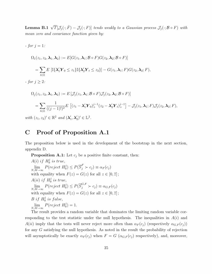
Lemma B.1√

T [Jj(·; F ) − Jj(·; F )] tends weakly to a Gaussian process Jj(·;B F ) with

mean zero and covariance function given by:

- for j = 1:

Ω1(z1, z2, λ1, λ2) := E[G(z1, λ1;B F )G(z2, λ2;B F )]

=∑t∈Z

E [Iλ′1Y 0 ≤ z1Iλ′2Y t ≤ z2]−G(z1, λ1; F )G(z2, λ2; F ),

- for j ≥ 2:

Ωj(z1, z2, λ1, λ2) := E [Jj(z1, λ1;B F )Jj(z2, λ2;B F )]

=∑t∈Z

1

((j − 1)!)2E

[(z1 − λ′1Y 0)

j−1+ (z2 − λ′2Y t)

j−1+

]− Jj(z1, λ1; F )Jj(z2, λ2; F ),

with (z1, z2)′ ∈ R2 and (λ′1, λ

′2)′ ∈ L2.

C Proof of Proposition A.1

The proposition below is used in the development of the bootstrap in the next section,

appendix D.

Proposition A.1: Let cj be a positive finite constant, then:

A(i) if Hj0 is true,

limN,M→∞

P (reject Hj0) ≤ P (S

F

j cj) ≡ αF (cj)

with equality when F (z) = G(z) for all z ∈ [0, z] ;

A(ii) if Hj0 is true,

limN,M→∞

P (reject Hj0) ≤ P (S

G,F

j cj) ≡ αG,F (cj)

with equality when F (z) = G(z) for all z ∈ [0, z] ;

B if Hj0 is false,

limN,M→∞

P (reject Hj0) = 1.

The result provides a random variable that dominates the limiting random variable cor-

responding to the test statistic under the null hypothesis. The inequalities in A(i) and

A(ii) imply that the tests will never reject more often than αF (cj) (respectively αG,F (cj))

for any G satisfying the null hypothesis. As noted in the result the probability of rejection

will asymptotically be exactly αF (cj) when F = G (αG,F (cj) respectively), and, moreover,

35

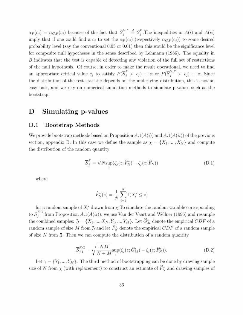
αF (cj) = αG,F (cj) because of the fact that SG,F

jd= S

F

j .The inequalities in A(i) and A(ii)

imply that if one could find a cj to set the αF (cj) (respectively αG,F (cj)) to some desired

probability level (say the conventional 0.05 or 0.01) then this would be the significance level

for composite null hypotheses in the sense described by Lehmann (1986). The equality in

B indicates that the test is capable of detecting any violation of the full set of restrictions

of the null hypothesis. Of course, in order to make the result operational, we need to find

an appropriate critical value cj to satisfy P (SF

j cj) ≡ α or P (SG,F

j cj) ≡ α. Since

the distribution of the test statistic depends on the underlying distribution, this is not an

easy task, and we rely on numerical simulation methods to simulate p-values such as the

bootstrap.

D Simulating p-values

D.1 Bootstrap Methods

We provide bootstrap methods based on Proposition A.1(A(i)) and A.1(A(ii)) of the previous

section, appendix B. In this case we define the sample as χ = X1, ...., XN and compute

the distribution of the random quantity

SF

j =√

Nsupz

(ζj(z; F ∗N)− ζj(z; FN)) (D.1)

where

F ∗N(z) =

1

N

N∑i=1

I(X∗i ≤ z)

for a random sample of X∗i drawn from χ.To simulate the random variable corresponding

to SF,G

j from Proposition A.1(A(ii)), we use Van der Vaart and Wellner (1996) and resample

the combined samples: Z = X1, ..., XN , Y1, ..., YM. Let G∗M denote the empirical CDF of a

random sample of size M from Z and let F ∗N denote the empirical CDF of a random sample

of size N from Z. Then we can compute the distribution of a random quantity

SF,G

j,1 =

√NM

N + Msup

z(ζj(z; G∗

M)− ζj(z; F ∗N)). (D.2)

Let γ = Y1, ..., YM. The third method of bootstrapping can be done by drawing sample

size of N from χ (with replacement) to construct an estimate of F ∗N and drawing samples of

36

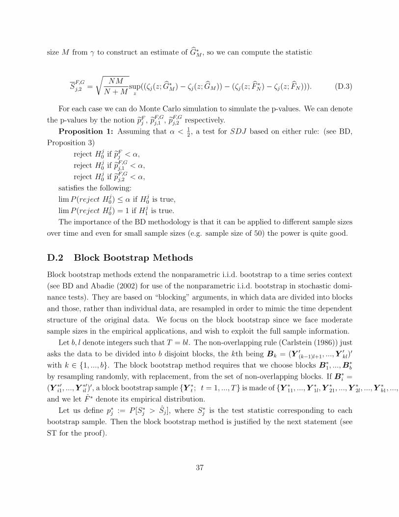
size M from γ to construct an estimate of G∗M , so we can compute the statistic

SF,G

j,2 =

√NM

N + Msup

z((ζj(z; G∗

M)− ζj(z; GM))− (ζj(z; F ∗N)− ζj(z; FN))). (D.3)

For each case we can do Monte Carlo simulation to simulate the p-values. We can denote

the p-values by the notion pFj , pF,G

j,1 , pF,Gj,2 respectively.

Proposition 1: Assuming that α < 12, a test for SDJ based on either rule: (see BD,

Proposition 3)

reject Hj0 if pF

j < α,

reject Hj0 if pF,G

j,1 < α,

reject Hj0 if pF,G

j,2 < α,

satisfies the following:

lim P (reject Hj0) ≤ α if Hj

0 is true,

lim P (reject Hj0) = 1 if Hj

1 is true.

The importance of the BD methodology is that it can be applied to different sample sizes

over time and even for small sample sizes (e.g. sample size of 50) the power is quite good.

D.2 Block Bootstrap Methods

Block bootstrap methods extend the nonparametric i.i.d. bootstrap to a time series context

(see BD and Abadie (2002) for use of the nonparametric i.i.d. bootstrap in stochastic domi-

nance tests). They are based on “blocking” arguments, in which data are divided into blocks

and those, rather than individual data, are resampled in order to mimic the time dependent

structure of the original data. We focus on the block bootstrap since we face moderate

sample sizes in the empirical applications, and wish to exploit the full sample information.

Let b, l denote integers such that T = bl. The non-overlapping rule (Carlstein (1986)) just

asks the data to be divided into b disjoint blocks, the kth being Bk = (Y ′(k−1)l+1, ...,Y

′kl)

′

with k ∈ 1, ..., b. The block bootstrap method requires that we choose blocks B∗1, ...,B

∗b

by resampling randomly, with replacement, from the set of non-overlapping blocks. If B∗i =

(Y ∗′i1, ...,Y

∗′il )

′, a block bootstrap sample Y ∗t ; t = 1, ..., T is made of Y ∗

11, ...,Y∗1l, Y

∗21, ...,Y

∗2l, ...,Y

∗b1, ...,Y

∗bl

and we let F ∗ denote its empirical distribution.

Let us define p∗j := P [S∗j > Sj], where S∗j is the test statistic corresponding to each

bootstrap sample. Then the block bootstrap method is justified by the next statement (see

ST for the proof).

37

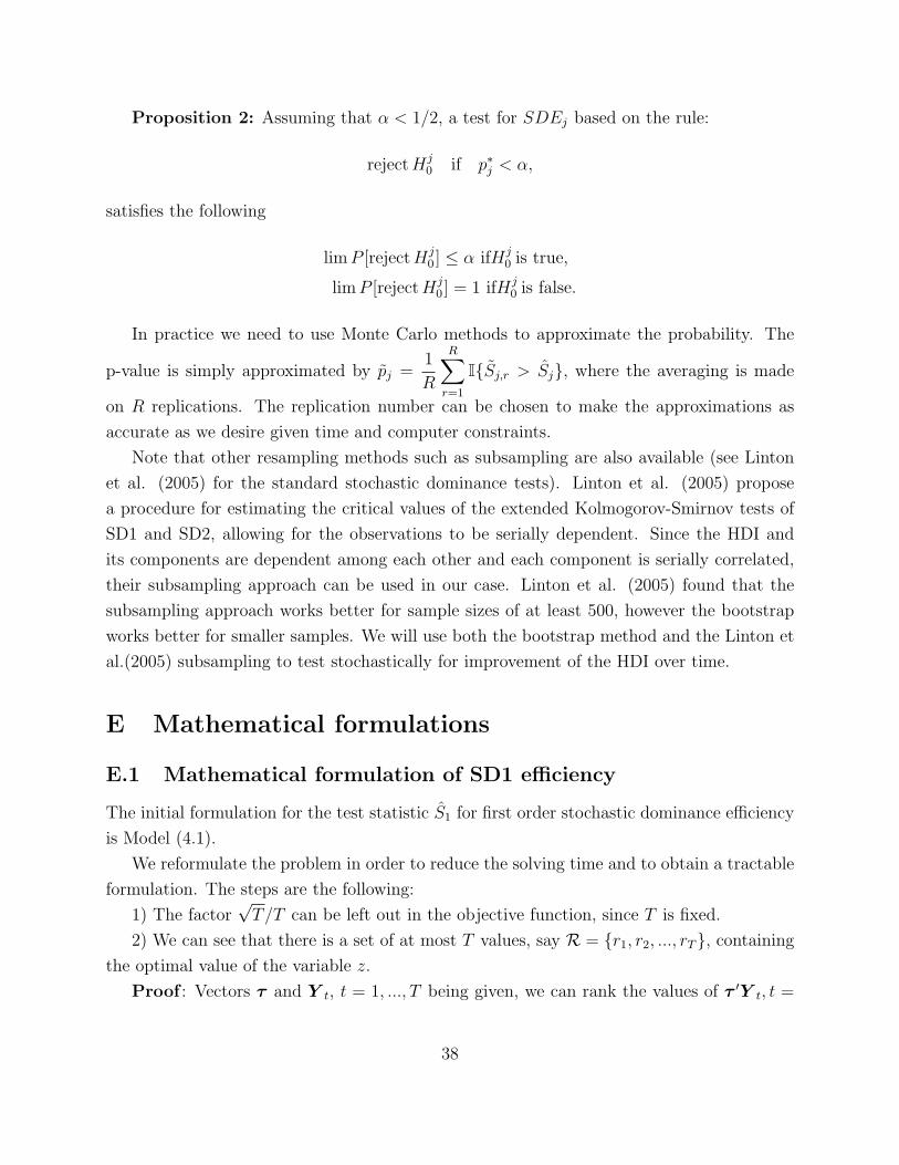
Proposition 2: Assuming that α < 1/2, a test for SDEj based on the rule:

reject Hj0 if p∗j < α,

satisfies the following

lim P [reject Hj0 ] ≤ α ifHj

0 is true,

lim P [reject Hj0 ] = 1 ifHj

0 is false.

In practice we need to use Monte Carlo methods to approximate the probability. The

p-value is simply approximated by pj =1

R

R∑r=1

ISj,r > Sj, where the averaging is made

on R replications. The replication number can be chosen to make the approximations as

accurate as we desire given time and computer constraints.

Note that other resampling methods such as subsampling are also available (see Linton

et al. (2005) for the standard stochastic dominance tests). Linton et al. (2005) propose

a procedure for estimating the critical values of the extended Kolmogorov-Smirnov tests of

SD1 and SD2, allowing for the observations to be serially dependent. Since the HDI and

its components are dependent among each other and each component is serially correlated,

their subsampling approach can be used in our case. Linton et al. (2005) found that the

subsampling approach works better for sample sizes of at least 500, however the bootstrap

works better for smaller samples. We will use both the bootstrap method and the Linton et

al.(2005) subsampling to test stochastically for improvement of the HDI over time.

E Mathematical formulations

E.1 Mathematical formulation of SD1 efficiency

The initial formulation for the test statistic S1 for first order stochastic dominance efficiency

is Model (4.1).

We reformulate the problem in order to reduce the solving time and to obtain a tractable

formulation. The steps are the following:

1) The factor√

T/T can be left out in the objective function, since T is fixed.

2) We can see that there is a set of at most T values, say R = r1, r2, ..., rT, containing

the optimal value of the variable z.

Proof : Vectors τ and Y t, t = 1, ..., T being given, we can rank the values of τ ′Y t, t =

38

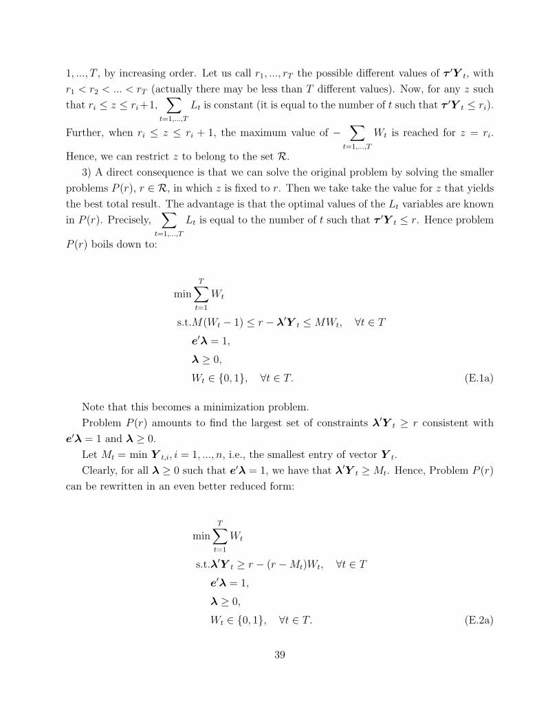
1, ..., T , by increasing order. Let us call r1, ..., rT the possible different values of τ ′Y t, with

r1 < r2 < ... < rT (actually there may be less than T different values). Now, for any z such

that ri ≤ z ≤ ri +1,∑

t=1,...,T

Lt is constant (it is equal to the number of t such that τ ′Y t ≤ ri).

Further, when ri ≤ z ≤ ri + 1, the maximum value of −∑

t=1,...,T

Wt is reached for z = ri.

Hence, we can restrict z to belong to the set R.

3) A direct consequence is that we can solve the original problem by solving the smaller

problems P (r), r ∈ R, in which z is fixed to r. Then we take take the value for z that yields

the best total result. The advantage is that the optimal values of the Lt variables are known

in P (r). Precisely,∑

t=1,...,T

Lt is equal to the number of t such that τ ′Y t ≤ r. Hence problem

P (r) boils down to:

minT∑

t=1

Wt

s.t.M(Wt − 1) ≤ r − λ′Y t ≤ MWt, ∀t ∈ T

e′λ = 1,

λ ≥ 0,

Wt ∈ 0, 1, ∀t ∈ T. (E.1a)

Note that this becomes a minimization problem.

Problem P (r) amounts to find the largest set of constraints λ′Y t ≥ r consistent with

e′λ = 1 and λ ≥ 0.

Let Mt = min Y t,i, i = 1, ..., n, i.e., the smallest entry of vector Y t.

Clearly, for all λ ≥ 0 such that e′λ = 1, we have that λ′Y t ≥ Mt. Hence, Problem P (r)

can be rewritten in an even better reduced form:

minT∑

t=1

Wt

s.t.λ′Y t ≥ r − (r −Mt)Wt, ∀t ∈ T

e′λ = 1,

λ ≥ 0,

Wt ∈ 0, 1, ∀t ∈ T. (E.2a)

39

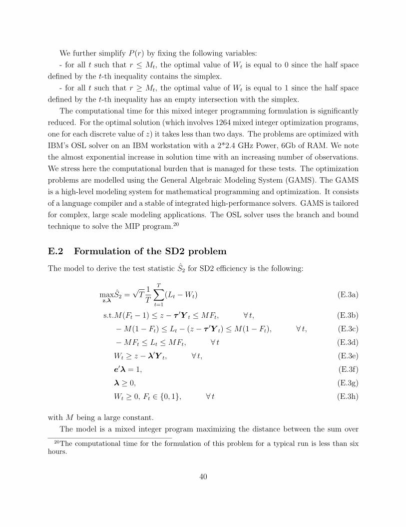
We further simplify P (r) by fixing the following variables:

- for all t such that r ≤ Mt, the optimal value of Wt is equal to 0 since the half space

defined by the t-th inequality contains the simplex.

- for all t such that r ≥ Mt, the optimal value of Wt is equal to 1 since the half space

defined by the t-th inequality has an empty intersection with the simplex.

The computational time for this mixed integer programming formulation is significantly

reduced. For the optimal solution (which involves 1264 mixed integer optimization programs,

one for each discrete value of z) it takes less than two days. The problems are optimized with

IBM’s OSL solver on an IBM workstation with a 2*2.4 GHz Power, 6Gb of RAM. We note

the almost exponential increase in solution time with an increasing number of observations.

We stress here the computational burden that is managed for these tests. The optimization

problems are modelled using the General Algebraic Modeling System (GAMS). The GAMS

is a high-level modeling system for mathematical programming and optimization. It consists

of a language compiler and a stable of integrated high-performance solvers. GAMS is tailored

for complex, large scale modeling applications. The OSL solver uses the branch and bound

technique to solve the MIP program.20

E.2 Formulation of the SD2 problem

The model to derive the test statistic S2 for SD2 efficiency is the following:

maxz,λ

S2 =√

T1

T

T∑t=1

(Lt −Wt) (E.3a)

s.t.M(Ft − 1) ≤ z − τ ′Y t ≤ MFt, ∀ t, (E.3b)

−M(1− Ft) ≤ Lt − (z − τ ′Y t) ≤ M(1− Ft), ∀ t, (E.3c)

−MFt ≤ Lt ≤ MFt, ∀ t (E.3d)

Wt ≥ z − λ′Y t, ∀ t, (E.3e)

e′λ = 1, (E.3f)

λ ≥ 0, (E.3g)

Wt ≥ 0, Ft ∈ 0, 1, ∀ t (E.3h)

with M being a large constant.

The model is a mixed integer program maximizing the distance between the sum over

20The computational time for the formulation of this problem for a typical run is less than sixhours.

40

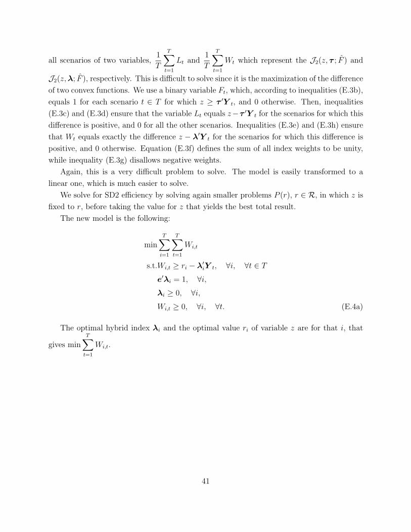
all scenarios of two variables,1

T

T∑t=1

Lt and1

T

T∑t=1

Wt which represent the J2(z, τ ; F ) and

J2(z, λ; F ), respectively. This is difficult to solve since it is the maximization of the difference

of two convex functions. We use a binary variable Ft, which, according to inequalities (E.3b),

equals 1 for each scenario t ∈ T for which z ≥ τ ′Y t, and 0 otherwise. Then, inequalities

(E.3c) and (E.3d) ensure that the variable Lt equals z−τ ′Y t for the scenarios for which this

difference is positive, and 0 for all the other scenarios. Inequalities (E.3e) and (E.3h) ensure

that Wt equals exactly the difference z − λ′Y t for the scenarios for which this difference is

positive, and 0 otherwise. Equation (E.3f) defines the sum of all index weights to be unity,

while inequality (E.3g) disallows negative weights.

Again, this is a very difficult problem to solve. The model is easily transformed to a

linear one, which is much easier to solve.

We solve for SD2 efficiency by solving again smaller problems P (r), r ∈ R, in which z is

fixed to r, before taking the value for z that yields the best total result.

The new model is the following:

minT∑

i=1

T∑t=1

Wi,t

s.t.Wi,t ≥ ri − λ′iY t, ∀i, ∀t ∈ T

e′λi = 1, ∀i,λi ≥ 0, ∀i,Wi,t ≥ 0, ∀i, ∀t. (E.4a)

The optimal hybrid index λi and the optimal value ri of variable z are for that i, that

gives minT∑

t=1

Wi,t.

41

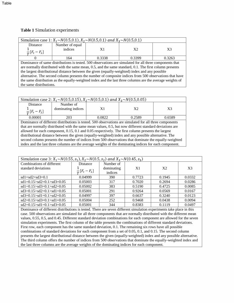
Table 1 Simulation experiments

Simulation case 1: Distance

Number of equal

indices

X1

X2

X3

0 164 0.3338 0.3399 0.3263

Dominance of same distributions is tested. 500 observations are simulated for all three components that

are normally distributed with the same mean, 0.5, and the same standard, 0.1. The first column presents

the largest distributional distance between the given (equally-weighted) index and any possible

alternative. The second column presents the number of composite indices from 500 observations that have

the same distribution as the equally-weighted index and the last three columns are the average weights of

the same distributions.

Simulation case 2: Distance

Number of

dominating indices

X1

X2

X3

0.00001 203 0.0822 0.2589 0.6589

Dominance of different distributions is tested. 500 observations are simulated for all three components

that are normally distributed with the same mean values, 0.5, but now different standard deviations are

allowed for each component, 0.15, 0.1 and 0.05 respectively. The first column presents the largest

distributional distance between the given (equally-weighted) index and any possible alternative. The

second column presents the number of indices from 500 observations that dominate the equally-weighted

index and the last three columns are the average weights of the dominating indices for each component.

Simulation case 3: Combinations of different

standard deviations

Distance

Number of

dominating

indices

X1

X2

X3

sd1=sd2=sd3=0.1 0.04999 390 0.7723 0.1945 0.0332

sd1=0.15>sd2=0.1>sd3=0.05 0.05003 317 0.7020 0.2694 0.0286

sd1=0.15>sd3=0.1>sd2=0.05 0.05002 383 0.5190 0.4725 0.0085

sd3=0.15>sd2=0.1>sd1=0.05 0.05001 291 0.9264 0.0569 0.0167

sd3=0.15>sd1=0.1>sd2=0.05 0.04997 397 0.6637 0.3240 0.0123

sd2=0.15>sd3=0.1>sd1=0.05 0.05004 252 0.9468 0.0438 0.0094

sd2=0.15>sd1=0.1>sd3=0.05 0.05001 344 0.8383 0.1119 0.0497

Dominance of different distributions is tested. There are seven different simulation experiments take place in this

case. 500 observations are simulated for all three components that are normally distributed with the different mean values, 0.55, 0.5, and 0.45. Different standard deviation combinations for each component are allowed for the seven

simulation experiments. The first column of the table presents the combinations of different standard deviations.

First row, each component has the same standard deviation, 0.1. The remaining six rows have all possible

combinations of standard deviations for each component from a set of 0.05, 0.1, and 0.15. The second column

presents the largest distributional distance between the given (equally-weighted) index and any possible alternative.

The third column offers the number of indices from 500 observations that dominate the equally-weighted index and

the last three columns are the average weights of the dominating indices for each component.

Table

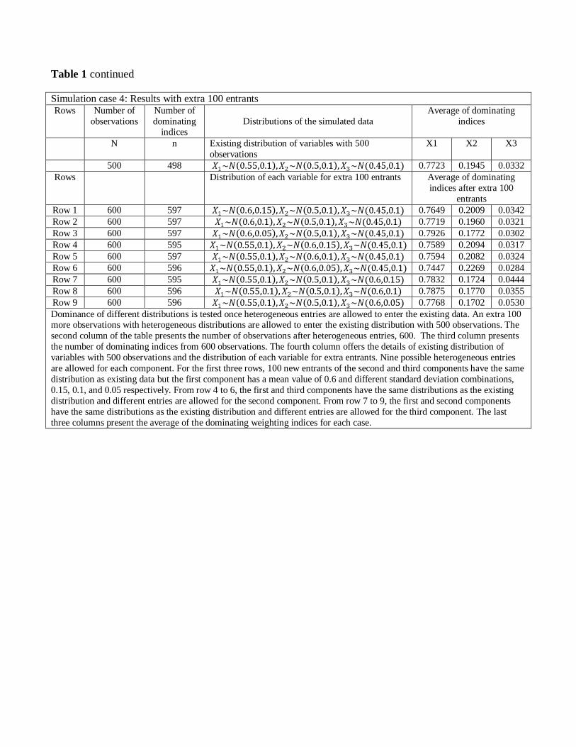
Table 1 continued

Simulation case 4: Results with extra 100 entrants Rows Number of

observations

Number of

dominating indices

Distributions of the simulated data

Average of dominating

indices

N n Existing distribution of variables with 500

observations

X1 X2 X3

500 498 0.7723 0.1945 0.0332

Rows Distribution of each variable for extra 100 entrants Average of dominating

indices after extra 100

entrants

Row 1 600 597 0.7649 0.2009 0.0342

Row 2 600 597 0.7719 0.1960 0.0321

Row 3 600 597 0.7926 0.1772 0.0302

Row 4 600 595 0.7589 0.2094 0.0317

Row 5 600 597 0.7594 0.2082 0.0324

Row 6 600 596 0.7447 0.2269 0.0284

Row 7 600 595 0.7832 0.1724 0.0444

Row 8 600 596 0.7875 0.1770 0.0355

Row 9 600 596 0.7768 0.1702 0.0530

Dominance of different distributions is tested once heterogeneous entries are allowed to enter the existing data. An extra 100 more observations with heterogeneous distributions are allowed to enter the existing distribution with 500 observations. The

second column of the table presents the number of observations after heterogeneous entries, 600. The third column presents

the number of dominating indices from 600 observations. The fourth column offers the details of existing distribution of

variables with 500 observations and the distribution of each variable for extra entrants. Nine possible heterogeneous entries

are allowed for each component. For the first three rows, 100 new entrants of the second and third components have the same

distribution as existing data but the first component has a mean value of 0.6 and different standard deviation combinations,

0.15, 0.1, and 0.05 respectively. From row 4 to 6, the first and third components have the same distributions as the existing

distribution and different entries are allowed for the second component. From row 7 to 9, the first and second components

have the same distributions as the existing distribution and different entries are allowed for the third component. The last

three columns present the average of the dominating weighting indices for each case.

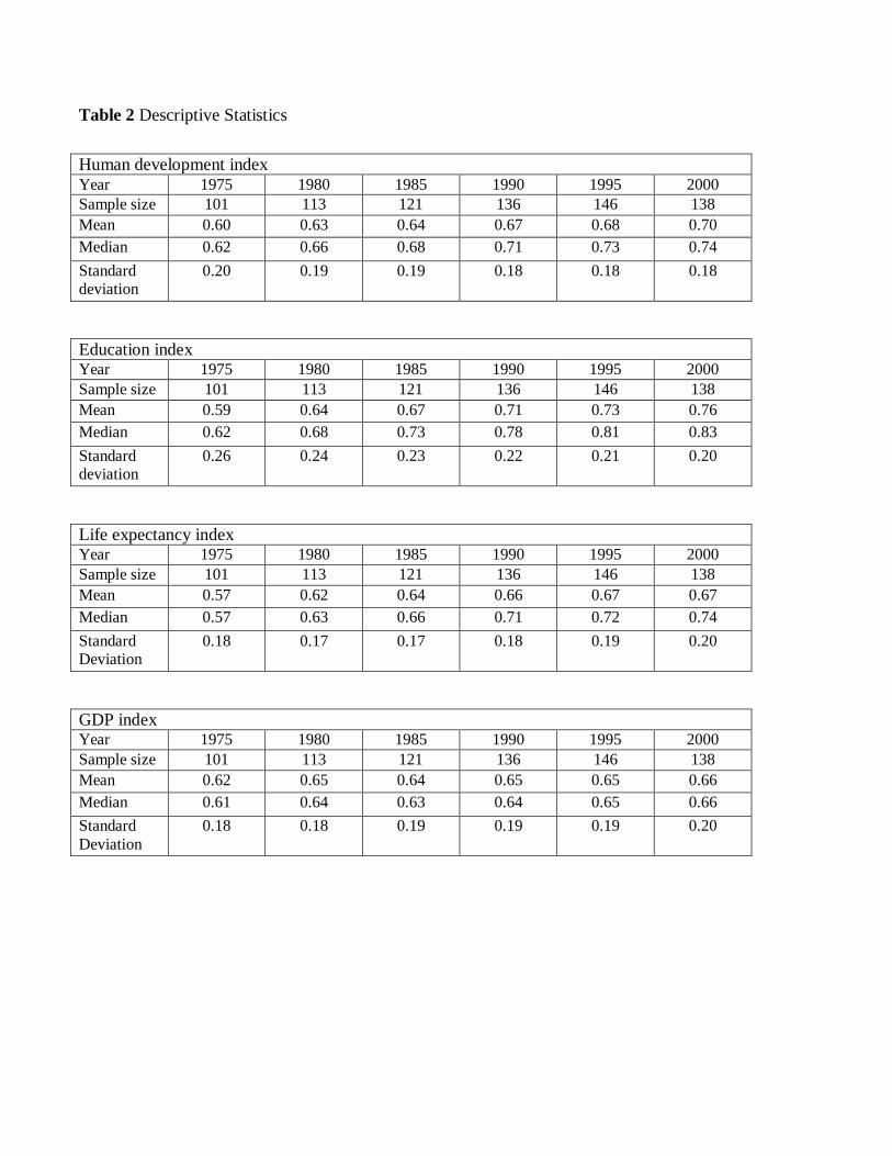
Table 2 Descriptive Statistics

Human development index Year 1975 1980 1985 1990 1995 2000

Sample size 101 113 121 136 146 138

Mean 0.60 0.63 0.64 0.67 0.68 0.70

Median 0.62 0.66 0.68 0.71 0.73 0.74

Standard deviation

0.20 0.19 0.19 0.18 0.18 0.18

Education index Year 1975 1980 1985 1990 1995 2000

Sample size 101 113 121 136 146 138

Mean 0.59 0.64 0.67 0.71 0.73 0.76

Median 0.62 0.68 0.73 0.78 0.81 0.83

Standard deviation

0.26 0.24 0.23 0.22 0.21 0.20

Life expectancy index Year 1975 1980 1985 1990 1995 2000

Sample size 101 113 121 136 146 138

Mean 0.57 0.62 0.64 0.66 0.67 0.67

Median 0.57 0.63 0.66 0.71 0.72 0.74

Standard Deviation

0.18 0.17 0.17 0.18 0.19 0.20

GDP index Year 1975 1980 1985 1990 1995 2000

Sample size 101 113 121 136 146 138

Mean 0.62 0.65 0.64 0.65 0.65 0.66

Median 0.61 0.64 0.63 0.64 0.65 0.66

Standard

Deviation

0.18 0.18 0.19 0.19 0.19 0.20

Table 3 Stochastic dominance results with BD (2003) sampling approach

Stochastic dominance results for education index

1975 1980 1985 1990 1995

1980 SD1 N/A - - - -

SD2 10% - - - -

1985 SD1 5% N/A - - -

SD2 1-5% N/A - - -

1990 SD1 1% 10% N/A - -

SD2 1% 1% 5-10% - -

1995 SD1 1% 5% 5% N/A -

SD2 1% 1% 1% N/A -

2000 SD1 1% 1% 1% 5% N/A

SD2 1% 1% 1% 1-5% 10% The vertical column represents the years from 1980 to 2000 that are tested for stochastic dominance

against years from 1975 to 1995. Percentage levels in the table represent the significance level of

stochastic dominance. N/A represents that there is no dominance at that order.

Stochastic dominance results for life expectancy index

1975 1980 1985 1990 1995

1980 SD1 N/A - - - -

SD2 1-5% - - - -

1985 SD1 5% N/A - - -

SD2 1% N/A - - -

1990 SD1 1% 5% N/A - -

SD2 1% 1-5% N/A - -

1995 SD1 1% 1% 5% N/A -

SD2 1% 1-5% 10% N/A -

2000 SD1 1% 1% 5% 10% N/A

SD2 1% 1% 10% 10% N/A The vertical column represents the years from 1980 to 2000 that are tested for stochastic dominance

against years from 1975 to 1995. Percentage levels in the table represent the significance level of stochastic dominance. N/A represents that there is no dominance at that order.

Stochastic dominance results for human development index

1975 1980 1985 1990 1995

1980 SD1 N/A - - - -

SD2 10% - - - -

1985 SD1 N/A N/A - - -

SD2 1-5% N/A - - -

1990 SD1 1% N/A N/A - -

SD2 1-5% 5-10% N/A - -

1995 SD1 1% 10% 10% N/A -

SD2 1% 5% 10% N/A -

2000 SD1 1% 5% 1% 10% N/A

SD2 1% 1% 1% 10% N/A The vertical column represents the years from 1980 to 2000 that are tested for stochastic dominance

against years from 1975 to 1995. Percentage levels in the table represent the significance level of

stochastic dominance. N/A represents that there is no dominance at that order.

Table 3 continued

Stochastic dominance results for GDP index

1975 1980 1985 1990 1995

1980 SD1 N/A - - - -

SD2 N/A - - - -

1985 SD1 N/A N/A - - -

SD2 N/A N/A - - -

1990 SD1 N/A N/A N/A - -

SD2 N/A N/A N/A - -

1995 SD1 N/A N/A N/A N/A -

SD2 N/A N/A N/A N/A -

2000 SD1 N/A N/A N/A N/A N/A

SD2 5-10% N/A N/A N/A N/A The vertical column represents the years from 1980 to 2000 that are tested for stochastic dominance

against years from 1975 to 1995. Percentage levels in the table represent the significance level of

stochastic dominance. N/A represents that there is no dominance at that order.

Table 4 Stochastic dominance results with Linton et al. (2005) subsampling approach

Stochastic dominance results for human development index

1975 1980 1985 1990 1995

1980 SD1 0.896 - - - -

SD2 0.582 - - - -

1985 SD1 0.892 0.837 - - -

SD2 0.441 0.569 - - -

1990 SD1 0.885 0.884 0.801 - -

SD2 0.557 0.437 0.470 - -

1995 SD1 0.517 0.941 0.797 0.535 -

SD2 0.420 0.532 0.555 0.804 -

2000 SD1 0.758 0.936 0.915 0.768 0.870

SD2 0.416 0.439 0.519 0.424 0.447 The vertical column represents the years from 1980 to 2000 that are tested for stochastic dominance against years

from 1975 to 1995. P-values for the null hypothesis that the given index in the following years dominates the index

of the previous years are reported.

Stochastic dominance results for education index

1975 1980 1985 1990 1995

1980 SD1 0.814 - - - -

SD2 0.402 - - - -

1985 SD1 0.856 0.880 - - -

SD2 0.401 0.604 - - -

1990 SD1 0.720 0.795 0.844 - -

SD2 0.448 0.584 0.729 - -

1995 SD1 0.582 0.830 0.990 0.000 -

SD2 0.552 0.405 0.735 0.364 -

2000 SD1 0.821 0.622 0.989 0.547 0.879

SD2 0.510 0.535 0.711 0.861 0.863 The vertical column represents the years from 1980 to 2000 that are tested for stochastic dominance against years

from 1975 to 199. P-values for the null hypothesis that the given index in the following years dominates the index of

the previous years are reported.

Stochastic dominance results for life expectancy index

1975 1980 1985 1990 1995

1980 SD1 0.995 - - - -

SD2 0.386 - - - -

1985 SD1 0.517 0.866 - - -

SD2 0.387 0.371 - - -

1990 SD1 0.650 0.650 0.018 - -

SD2 0.611 0.582 0.018 - -

1995 SD1 0.650 0.570 0.803 0.031 -

SD2 0.479 0.521 0.598 0.000 -

2000 SD1 0.569 0.490 0.557 0.004 0.012

SD2 0.541 0.555 0.521 0.000 0.000 The vertical column represents the years from 1980 to 2000 that are tested for stochastic dominance against years

from 1975 to 1995. P-values for the null hypothesis that the given index in the following years dominates the index

of the previous years are reported.

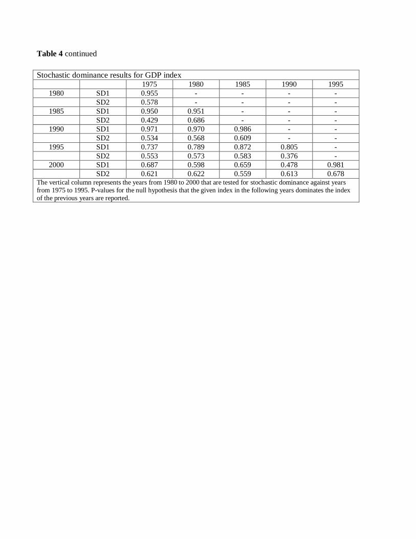
Table 4 continued

Stochastic dominance results for GDP index

1975 1980 1985 1990 1995

1980 SD1 0.955 - - - -

SD2 0.578 - - - -

1985 SD1 0.950 0.951 - - -

SD2 0.429 0.686 - - -

1990 SD1 0.971 0.970 0.986 - -

SD2 0.534 0.568 0.609 - -

1995 SD1 0.737 0.789 0.872 0.805 -

SD2 0.553 0.573 0.583 0.376 -

2000 SD1 0.687 0.598 0.659 0.478 0.981

SD2 0.621 0.622 0.559 0.613 0.678 The vertical column represents the years from 1980 to 2000 that are tested for stochastic dominance against years

from 1975 to 1995. P-values for the null hypothesis that the given index in the following years dominates the index

of the previous years are reported.

Table 5 Stochastic efficient weighting for human development index

Stochastic efficient weighting for human development index

Stochastic efficient weights

Highest distance

Number of indices that

dominate fixed

weighted HDI

Life

expectancy

index

Education

index

GDP

index

0.04540 293 0.1238 0.7117 0.1645

Stochastic efficient weights of life expectancy, educational attainment and standard of living that dominate the equally-weighted HDI are presented. Highest distance obtained

between any alternative composite index and the equally-weighted HDI empirical

distributions is given. There are 293 composite indices that dominate the equally-

weighted index. The average of dominating indices offer the stochastic efficient weights assigned to each component.

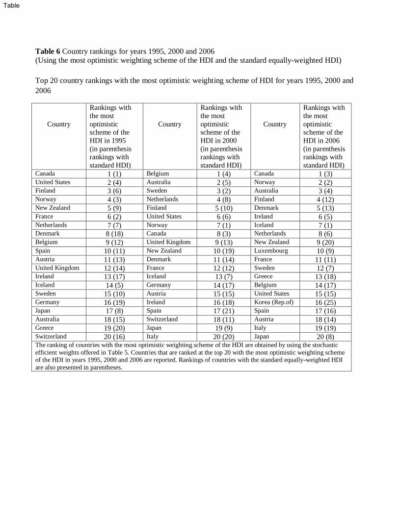
Table 6 Country rankings for years 1995, 2000 and 2006

(Using the most optimistic weighting scheme of the HDI and the standard equally-weighted HDI)

Top 20 country rankings with the most optimistic weighting scheme of HDI for years 1995, 2000 and

2006

Country

Rankings with

the most

optimistic scheme of the

HDI in 1995

(in parenthesis rankings with

standard HDI)

Country

Rankings with

the most

optimistic scheme of the

HDI in 2000

(in parenthesis rankings with

standard HDI)

Country

Rankings with

the most

optimistic scheme of the

HDI in 2006

(in parenthesis rankings with

standard HDI) Canada 1 (1) Belgium 1 (4) Canada 1 (3) United States 2 (4) Australia 2 (5) Norway 2 (2) Finland 3 (6) Sweden 3 (2) Australia 3 (4) Norway 4 (3) Netherlands 4 (8) Finland 4 (12) New Zealand 5 (9) Finland 5 (10) Denmark 5 (13) France 6 (2) United States 6 (6) Ireland 6 (5) Netherlands 7 (7) Norway 7 (1) Iceland 7 (1) Denmark 8 (18) Canada 8 (3) Netherlands 8 (6) Belgium 9 (12) United Kingdom 9 (13) New Zealand 9 (20) Spain 10 (11) New Zealand 10 (19) Luxembourg 10 (9) Austria 11 (13) Denmark 11 (14) France 11 (11) United Kingdom 12 (14) France 12 (12) Sweden 12 (7) Ireland 13 (17) Iceland 13 (7) Greece 13 (18) Iceland 14 (5) Germany 14 (17) Belgium 14 (17) Sweden 15 (10) Austria 15 (15) United States 15 (15) Germany 16 (19) Ireland 16 (18) Korea (Rep.of) 16 (25) Japan 17 (8) Spain 17 (21) Spain 17 (16) Australia 18 (15) Switzerland 18 (11) Austria 18 (14) Greece 19 (20) Japan 19 (9) Italy 19 (19) Switzerland 20 (16) Italy 20 (20) Japan 20 (8) The ranking of countries with the most optimistic weighting scheme of the HDI are obtained by using the stochastic

efficient weights offered in Table 5. Countries that are ranked at the top 20 with the most optimistic weighting scheme of the HDI in years 1995, 2000 and 2006 are reported. Rankings of countries with the standard equally-weighted HDI

are also presented in parentheses.

Table

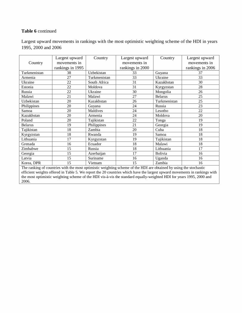
Table 6 continued

Largest upward movements in rankings with the most optimistic weighting scheme of the HDI in years

1995, 2000 and 2006

Country

Largest upward movements in

rankings in 1995

Country Largest upward movements in

rankings in 2000

Country Largest upward movements in

rankings in 2006 Turkmenistan 38 Uzbekistan 33 Guyana 37

Armenia 27 Turkmenistan 33 Ukraine 33

Ukraine 22 South Africa 31 Kazakhstan 30

Estonia 22 Moldova 31 Kyrgyzstan 28

Russia 22 Ukraine 30 Mongolia 26

Malawi 21 Malawi 27 Belarus 25

Uzbekistan 20 Kazakhstan 26 Turkmenistan 25

Philippines 20 Guyana 24 Russia 23

Samoa 20 Maldives 24 Lesotho 22

Kazakhstan 20 Armenia 24 Moldova 20

Poland 20 Tajikistan 22 Tonga 19

Belarus 19 Philippines 21 Georgia 19

Tajikistan 18 Zambia 20 Cuba 18

Kyrgyzstan 18 Rwanda 19 Samoa 18

Lithuania 17 Kyrgyzstan 19 Tajikistan 18

Grenada 16 Ecuador 18 Malawi 18

Zimbabwe 15 Russia 18 Lithuania 17

Georgia 15 Azerbaijan 17 Bolivia 16

Latvia 15 Suriname 16 Uganda 16

Korea, DPR 15 Vietnam 15 Zambia 16

The ranking of countries with the most optimistic weighting scheme of the HDI are obtained by using the stochastic

efficient weights offered in Table 5. We report the 20 countries which have the largest upward movements in rankings with

the most optimistic weighting scheme of the HDI vis-à-vis the standard equally-weighted HDI for years 1995, 2000 and

2006.

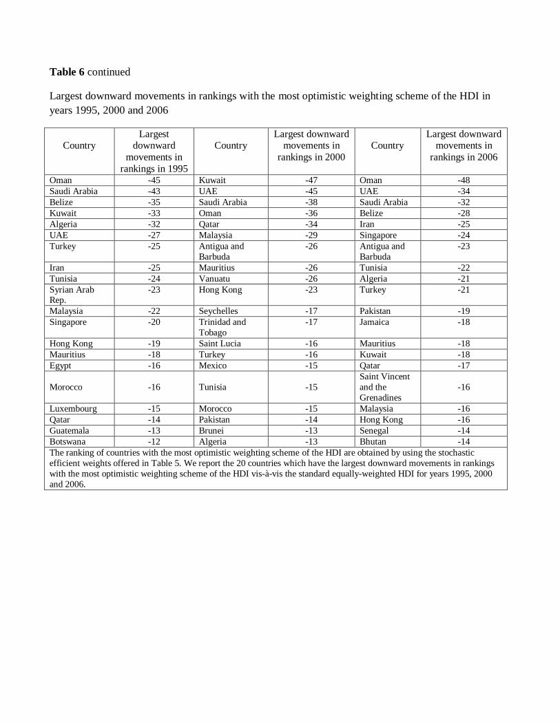
Table 6 continued

Largest downward movements in rankings with the most optimistic weighting scheme of the HDI in

years 1995, 2000 and 2006

Country

Largest downward

movements in

rankings in 1995

Country

Largest downward movements in

rankings in 2000

Country

Largest downward movements in

rankings in 2006

Oman -45 Kuwait -47 Oman -48

Saudi Arabia -43 UAE -45 UAE -34

Belize -35 Saudi Arabia -38 Saudi Arabia -32

Kuwait -33 Oman -36 Belize -28

Algeria -32 Qatar -34 Iran -25

UAE -27 Malaysia -29 Singapore -24

Turkey -25 Antigua and

Barbuda

-26 Antigua and

Barbuda

-23

Iran -25 Mauritius -26 Tunisia -22

Tunisia -24 Vanuatu -26 Algeria -21

Syrian Arab Rep.

-23 Hong Kong -23 Turkey -21

Malaysia -22 Seychelles -17 Pakistan -19

Singapore -20 Trinidad and

Tobago

-17 Jamaica -18

Hong Kong -19 Saint Lucia -16 Mauritius -18

Mauritius -18 Turkey -16 Kuwait -18

Egypt -16 Mexico -15 Qatar -17

Morocco

-16

Tunisia

-15

Saint Vincent

and the

Grenadines

-16

Luxembourg -15 Morocco -15 Malaysia -16

Qatar -14 Pakistan -14 Hong Kong -16

Guatemala -13 Brunei -13 Senegal -14

Botswana -12 Algeria -13 Bhutan -14

The ranking of countries with the most optimistic weighting scheme of the HDI are obtained by using the stochastic

efficient weights offered in Table 5. We report the 20 countries which have the largest downward movements in rankings

with the most optimistic weighting scheme of the HDI vis-à-vis the standard equally-weighted HDI for years 1995, 2000

and 2006.

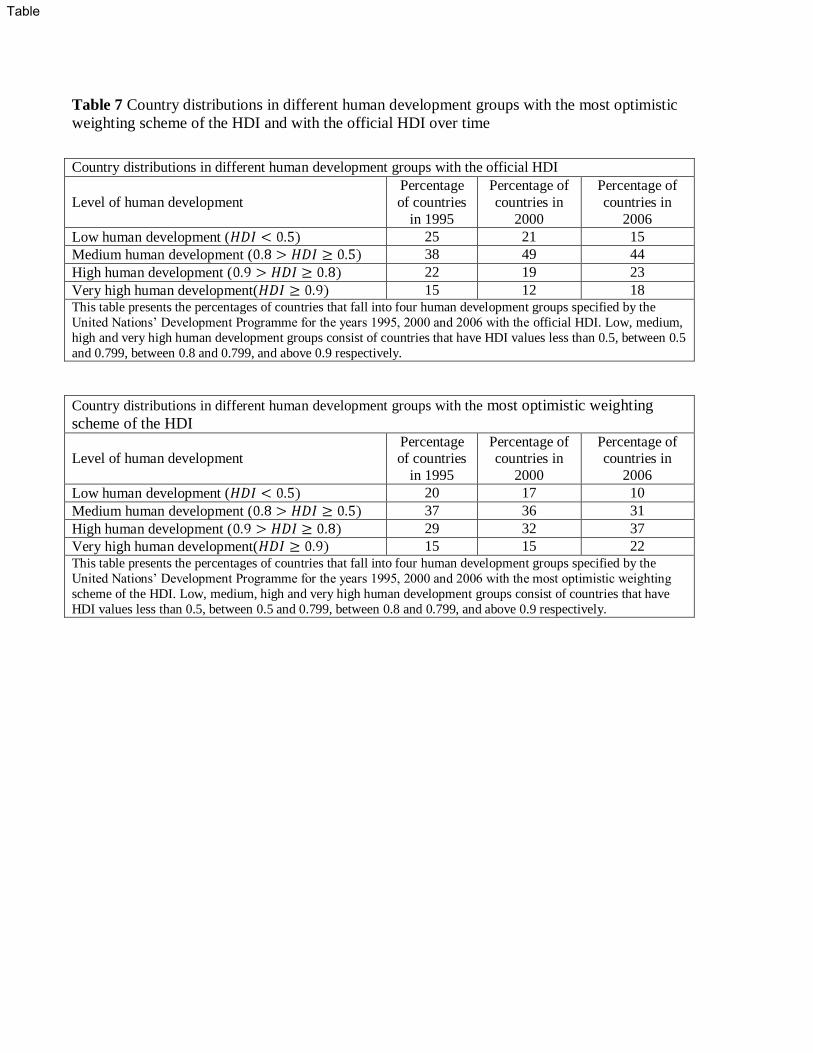
Table 7 Country distributions in different human development groups with the most optimistic

weighting scheme of the HDI and with the official HDI over time

Country distributions in different human development groups with the official HDI

Level of human development

Percentage

of countries

in 1995

Percentage of

countries in

2000

Percentage of

countries in

2006

Low human development ( 25 21 15

Medium human development ( 38 49 44

High human development ( 22 19 23

Very high human development( 15 12 18 This table presents the percentages of countries that fall into four human development groups specified by the

United Nations’ Development Programme for the years 1995, 2000 and 2006 with the official HDI. Low, medium,

high and very high human development groups consist of countries that have HDI values less than 0.5, between 0.5

and 0.799, between 0.8 and 0.799, and above 0.9 respectively.

Country distributions in different human development groups with the most optimistic weighting

scheme of the HDI Level of human development

Percentage of countries

in 1995

Percentage of countries in

2000

Percentage of countries in

2006

Low human development ( 20 17 10

Medium human development ( 37 36 31

High human development ( 29 32 37

Very high human development( 15 15 22 This table presents the percentages of countries that fall into four human development groups specified by the

United Nations’ Development Programme for the years 1995, 2000 and 2006 with the most optimistic weighting

scheme of the HDI. Low, medium, high and very high human development groups consist of countries that have

HDI values less than 0.5, between 0.5 and 0.799, between 0.8 and 0.799, and above 0.9 respectively.

Table