Measuring the Robustness of Resource Allocationsin a Stochastic Dynamic Environment

Jay Smith1,2, Luis D. Briceno2, Anthony A. Maciejewski2, Howard Jay Siegel2,3,Timothy Renner3, Vladimir Shestak2, Joshua Ladd4, Andrew Sutton3, David Janovy2,

Sudha Govindasamy2, Amin Alqudah2, Rinku Dewri3, Puneet Prakash2 ∗

1IBM Colorado State University6300 Diagonal Highway 2Dept. of Electrical Engineering

Boulder, CO 80301 3Dept. of Computer Sciencebigfun@us.ibm.com 4Mathematics Department

Fort Collins, CO 80523–1373 USA{ldbricen,aam,hj}@colostate.edu

Abstract

Heterogeneous distributed computing systems often mustoperate in an environment where system parameters aresubject to uncertainty. Robustness can be defined as thedegree to which a system can function correctly in the pres-ence of parameter values different from those assumed. Wepresent a methodology for quantifying the robustness of re-source allocations in a dynamic environment where task ex-ecution times are stochastic. The methodology is evaluatedthrough measuring the robustness of three different resourceallocation heuristics within the context of a stochastic dy-namic environment. A Bayesian regression model is fit to thecombined results of the three heuristics to demonstrate thecorrelation between the stochastic robustness metric andthe presented performance metric. The correlation resultsdemonstrated the significant potential of the stochastic ro-bustness metric to predict the relative performance of thethree heuristics given a common objective function.

1. Introduction

Heterogeneous parallel and distributed computing is de-fined as the coordinated use of compute resources that have

∗This research was supported by the NSF under Contract No: CNS-0615170, by the Colorado State University Center for Robustness in Com-puter Systems (funded by the Colorado Commission on Higher EducationTechnology Advancement Group through the Colorado Institute of Tech-nology), and by the Colorado State University George T. Abell Endow-ment.1-4244-0910-1/07/$20.00 c©2007 IEEE.

different capabilities to optimize system performance fea-tures. Often, heterogeneous, distributed computing sys-tems must operate in an environment replete with uncer-tainty. Robustness in this context can be defined as the de-gree to which a system can function correctly in the pres-ence of parameter values different from those assumed [1].We present the use of a stochastic robustness metric [14]to quantify the robustness of a resource allocation in a dy-namic environment. This formulation of the stochastic ro-bustness metric is used to predict the typical relative perfor-mance of three different resource allocation heuristics takenfrom the literature and adapted to the presented problem. ABayesian regression model is fit to the combined results ofthe three heuristics to demonstrate the relationship betweenthe stochastic robustness metric and the presented perfor-mance metric. The accuracy of the robustness predictionsare then evaluated to determine their utility in predictingresource allocation heuristic performance in a dynamic en-vironment.

The major contribution of this paper is a mathemat-ical formulation for quantifying the robustness of a re-source allocation in a stochastic dynamic environment anda methodology for applying the robustness formulation topredict heuristic performance. We demonstrate the pro-posed methodology by successfully predicting the relativeperformance of three heuristics taken from the literature andadapted to this environment. Finally, we present a detailedevaluation of the three heuristics using both the proposedrobustness metric and a performance objective appropriateto the studied environment.

The environment considered in this research is that ofa heterogeneous, distributed computing system designed to

service a high volume web site of world-wide interest. Thesystem being modeled was used to implement the 1998World Cup web site [3] that processed more than 1.3 bil-lion HTTP requests during the summer of 1998. The website was provided to a world-wide audience by four het-erogeneous, geographically dispersed systems—each withtheir own processing capacity and workload distributiontechniques. This class of system is very challenging toimplement but occurs surprisingly frequently. The WorldCup football tournament is just one example of an eventof world-wide appeal that necessitates web based cover-age. Sites of this type are typically constructed for specificevents and the volume of traffic is on the order of billionsof requests in a period of only a few months or less. Othersuch events might include the Summer Olympics, the Win-ter Olympics, or the tour de France; all are reasonably ex-pected to draw the attention of a world-wide audience in thebillions.

This research developed resource allocation heuristicsfor a single location of a distributed system capable ofprocessing a high volume of requests. Incoming requestswere dispersed to one of four processing centers. Thus,each location was responsible for processing some fractionof the total traffic to the site. This work focused on a loca-tion comprising eight heterogeneous servers responsible forprocessing 45% of the overall traffic [2].

A task is defined to be a menu-driven HTTP request fordata from the web site. Mapping tasks to machines in thisdistributed system is rather challenging as it must be doneunder uncertainty because the exact execution time requiredto process a task is not known a priori. However, past ob-servations of task execution times can be used to constructa probability mass function (pmf) [17] that models the pos-sible execution times for a given task. The pattern of taskarrivals to the site was modeled after real traffic patterns ob-served by the 1998 World Cup web site [2].

In the next section, we present the details of the problemto be addressed. Section 3 defines a means for determin-ing stochastic completion times for tasks in this system us-ing the details of the problem statement. The definition ofstochastic completion times is then used in Section 4 to de-rive a stochastic robustness metric that is subsequently usedto predict heuristic performance. In Section 5, we presentthe heuristics that have been developed as part of this re-search. Details of the simulation environment are presentedin Section 6 and the results of the heuristics are evaluatedin Section 7. Section 8 presents an overview of the relevantrelated work. Section 9 concludes the paper.

2. Problem Statement

2.1. Introduction

The system studied in this research is an instance of amore general class of dynamic, heterogeneous computing(HC) system where task arrival times are not known in ad-vance and exact task execution times are uncertain priorto their completion. All incoming tasks to the system areassumed to have been previously classified into one of Cclasses prior to their arrival. Each of the classes correspondsto a gross classification of the relative complexity of the re-quest being processed. Each task class defines a set of pmfs,where each pmf describes the probability of all executiontimes for that class on a given machine within the HC suite.Further, all of the classes of tasks (HTTP requests) that thesystem may be asked to perform are known in advance, i.e.,the web server has prior knowledge about what web pagesit is providing.

Each arriving task has a relative deadline limiting the to-tal time available to process each request. The relative dead-line for each task class is assumed to have been establishedin advance. Because tasks in this environment are HTTPrequests for data, made by a user of the website, it is as-sumed that if a task cannot be completed by its deadlinethen the request can be considered to be “timed out” andthe user that submitted the original request will make therequest again. Therefore, there is no benefit to completingtasks that miss their deadlines and, consequently, tasks thatmiss their deadlines will be discarded.

2.2. Performance Metric

In this environment, each incoming task has a hard dead-line for its completion, i.e., failure to complete a task by itsdeadline will result in a penalty. To model the impact ofmissing a task deadline the resource allocation heuristic willbe penalized by a constant factor of 1 for each task deadlinethat is missed. That is, for a given task iwith deadline βmax

i

let comp(i) be the actual completion time of task i and de-fine the cost to process a task i, denoted cost(i), as follows

cost(i) ={

0, if comp(i) ≤ βmaxi ;

1, otherwise. (1)

The overall cost of a resource allocation is defined as thesum of the cost of each processed task. Define PT as theset of all tasks that are processed by the system, then theobjective of a resource allocation in this environment canbe expressed as,

Minimize∑

∀i∈PT

cost(i). (2)

Intuitively, resource allocations in this environment are ex-pected to minimize the number of tasks that miss their dead-lines.

2.3. Mapping Events

All of the resource allocation heuristics evaluated in thiswork operate in a pseudo-batch mode [10,11]. In a pseudo-batch mode heuristic, all tasks that have not begun execu-tion and are not next in line to begin execution can be con-sidered for remapping when a mapping event occurs. Map-ping events occur within the system whenever a new taskarrives or an existing task completes.

3. Stochastic Task Completion Time

Although some tasks may belong to the same class, taskexecution times may still vary depending on the details ofthe data requested. For this reason, task execution times aremodeled as random variables. In addition, it is reasonableto assume that each task execution time is independent be-cause any single HTTP request can be satisfied without anyneed to process another HTTP request, i.e., each request isself-contained.

Let each task i belong to exactly one class ci in the set ofall task classifications C where membership in a class im-plies a specific random variable Tcij representing the execu-tion time of that task class on machine j (one of the M ma-chines in the HC suite). In this research, it is assumed thatthe probability distributions describing the random variableTcij were created from measurements of the response timesof actual requests for data from the site. A typical methodfor creating such a distribution relies on a histogram esti-mator [17] that produces a discrete probability distributionknown as a probability mass function. Define fcj to be aunimodal pmf describing the execution time of tasks in classc on machine j. We consider only unimodal distributions ofexecution times to simplify the application of the stochasticrobustness metric.

Determining the completion time for a machine j, andtherefore the completion time of a particular task i, requiresa means of combining the execution times for all tasks as-signed to that machine. In a deterministic model of taskexecution times, the estimated execution times for all tasksassigned to machine j would be summed with the machineready time to produce a completion time. A similar pro-cedure is followed in the stochastic case as well. How-ever, calculating stochastic completion times requires thesummation of random variables as opposed to determinis-tic values. The summation of random variables given theirpmfs can be found as the convolution of their correspondingpmfs [9].

Let MQ(t) be the set of all tasks that are either pend-ing execution or are currently executing on any of the Mmachines in the HC suite at time t. To determine the com-pletion time for a task i on machine j at time t, identify thesubset of tasks in MQ(t) that were mapped to machine jin advance of task i, denoted MQij(t). The execution timepmfs for the pending tasks will be convolved [9] with thecompletion time distribution of the currently executing taskand the execution time distribution for task i on machine jto produce the stochastic completion time pmf for task i onmachine j.

The execution time pmf for the currently executing taskon machine j requires some additional processing prior toits convolution with the pmfs of the pending tasks to createa completion time pmf. For example, if the currently exe-cuting task on machine j began execution at time tj priorto time t, some of the impulse values of the pmf describ-ing the completion time of the currently executing task maybe in the past. Therefore, to accurately describe the com-pletion time of task i at time t requires that these past im-pulses be removed from the pmf and the remaining distri-bution renormalized. After renormalization, the resultingdistribution describes the completion time of the currentlyexecuting task at time t on machine j. To simplify notation,define an operator GT (s, d) that accepts a scalar s and apmf d as input and returns a renormalized probability distri-bution where all impulse values of the returned distributionare greater than s. The completion time pmf of the currentlyexecuting task on machine j is determined by applying theGT operator to its completion time pmf, using the currenttime t. The resulting distribution is then convolved with thepmfs of the pending tasks on machine j and the executiontime distribution of task i to produce the completion timepmf for task i on machine j at the current time t.

4. Stochastic Robustness Metric (SRM) for aDynamic Mapper

4.1. Instantaneous SRM

Recall that the individual deadline of each task has beendefined in advance; let βmax

i denote the deadline for the ith

task to arrive to the system. Let fc1j be the execution timepmf of the currently executing task on machine j. Order themembers of MQij(t) according to their scheduled order ofexecution on machine j and let fc2j be the execution timepmf of the first pending task on machine j, with fc|MQij(t)|j

as the execution time pmf of the last pending task on ma-chine j that is ahead of task i.

Convolution of a scalar with a pmf has the effect of shift-ing the pmf by the value of the scalar and has no impact onthe distribution of probabilities in the pmf. Therefore, ifMQij(t) = ∅, i.e., MQij(t) is empty, the completion time

distribution for task i on machine j is merely its executiontime distribution fcij shifted to the current time. The com-pletion time distribution at time t for task i, denoted Fi(t)can be found as follows,

Fi(t) =

t ∗ fcij , if MQij(t) = ∅;

GT{t, tj ∗ fc1j} ∗ fc2j ∗ · · ·∗fc|MQij(t)| ∗ fcij , otherwise.

(3)Following from our prior work on robustness [14], the

robustness of the finishing time for task i can be found as theprobability that task i will finish before its deadline. Thisprobability defines a local robustness characteristic, denotedψi(t), and can be expressed as P

[Fi(t) ≤ βmax

i

]. The in-

dividual local robustness characteristics can then be com-bined to produce the stochastic robustness metric at time t,denoted ψ(t), as follows,

ψ(t) =∏

∀i∈MQ(t)

(P[Fi(t) ≤ βmax

i

]). (4)

This combination of local robustness characteristics de-fines an instantaneous measure of robustness (instantaneousSRM) for this resource allocation at a particular time t. In-tuitively, the measure defines the probability that all taskspending or currently executing at time t will meet theirdeadlines.

4.2. Dynamic SRM Value

The instantaneous measure of robustness is used as a ba-sis for defining a single dynamic SRM value. To define thatvalue, recall that a mapping event occurs whenever a taskcompletes execution or a new task arrives at the system.An instantaneous SRM value is generated at each mappingevent during the course of a simulation trial. These instan-taneous SRM values are then combined to create a sam-ple dynamic SRM value for the resource allocation heuris-tic. Given the relationship between the dynamic SRM valueand the performance metric, the dynamic SRM value canbe used to predict the relative performance of two resourceallocation heuristics.

If a heuristic consistently maintains a high ψ(t) valueover some number of mapping events then there is a con-sistently low probability that tasks will miss their deadlinesover that same period. Therefore, the average ψ(t) valueover a large enough number of mapping events should cor-relate with a consistently low probability that tasks will misstheir deadlines. That is, heuristics that maintain a high aver-age ψ(t) value can reasonably be expected to produce a lowcost. For this reason, the dynamic SRM value is defined asthe average of the instantaneous SRM values found, at eachmapping event, during a simulation trial.

4.3 Using the Dynamic SRM value

In a dynamic environment, the set of tasks being consid-ered is constantly changing due to task arrivals and com-pletions. Recall that to compute ψ(t) the start time of thecurrently executing task on each machine is required (i.e.,tj). Determing the start time for a task i requires knowledgeof the actual execution time of the previously executed taskk on that machine to calculate task k’s actual completiontime. During simulations used for heuristic evaluation, ourmethodology utilizes the expectation of the execution timepmf as the actual execution time for each task. Thus, thestart time of the subsequent task i is known, enabling thecalculation of ψ(t).

Taking the expectation of the class pmfs to produce themost likely actual execution times to use for the evaluationsimulations is reasonable in this environment because thetask execution time pmfs are assumed to be unimodal. Fur-ther study is required to determine the most effective ap-proach when execution time pmfs are not unimodal.

A second factor in evaluating a resource allocationheuristic is the set of tasks and the ordering of task arrivals.Because of variations in the set of tasks to be executed andchanges in their arrival ordering, multiple simulation trialsshould be conducted to adequately predict the typical rel-ative performance among the evaluated resource allocationheuristics. In evaluating our results, we will demonstratethat in a dynamic environment a small number of simulationtrials are required to sufficiently indicate the performance ofa resource allocation heuristic relative to our given perfor-mance objective. Each trial involves a unique set of taskswith a unique arrival order.

To produce a dynamic SRM value for a resource alloca-tion heuristic a relatively small number of simulations areexecuted where the mean of each task execution time distri-bution is used as the actual execution time. This producesa dynamic SRM value for each resource allocation (simu-lation trial) where the dynamic SRM value is determinedas the average of the instaneous SRM values within thatsimulation trial. The dynamic SRM values for all of thesimulation trials are then combined by taking their averageto determine a single dynamic SRM value for the resourceallocation heuristic.

The dynamic SRM values for different resource alloca-tion heuristics can then be compared to select the approachthat is more robust within the given environment. That is,given the presented formulation of the instantaneous SRM,a simulation trial that has a higher dynamic SRM valueshould reasonably be expected to produce fewer task dead-line misses. In the next section, we present the heuristicsthat are to be evaluated using the dynamic SRM value inSection 7.

5. Resource Allocation Heuristics to Evaluate

5.1. Introduction

The goal of resource allocation heuristics is to selecta mapping of tasks to machines and scheduling of taskswithin a machine that minimizes an objective function. Thepresented heuristics do not directly attempt to maximize thestochastic robustness metric, instead focusing on minimiz-ing the primary objective function. In the results section,the heuristics will be compared using both the stochasticrobustness metric and their average performance relative tominimizing Equation 2. All of the heuristics were given alimited amount of time to complete a mapping event.

5.2. Two Phase Greedy

The Two Phase Greedy heuristic is based on the princi-ples of the Min-Min algorithm (first presented in [8], andshown to perform well in many environments [7], [10],[15]). The heuristic allocates one task at each iteration, con-tinuing until all task allocations have been resolved. In thefirst phase of each iteration, the Two Phase Greedy heuris-tic determines the best assignment (according to the perfor-mance goal) for each of the tasks left unmapped. In the sec-ond phase, it selects the task to map based on the best resultfound in the first phase. The completion time distributionfor a given machine j at time t is denoted F j(t). Giventhe set of tasks assigned to machine j at time t, denotedMQj(t), F j(t) can be found as follows:

F j(t) = GT{t, tj ∗ fc1j} ∗ fc2j ∗ · · · ∗ fc|MQj(t)|. (5)

The Two Phase Greedy heuristic is summarized in Figure 1.

while not all tasks are mappedfor each unmapped task i

find machine mj such thatmj ← argmin

1≤j≤M

[E[F j(t) ∗ fcij ]

];

resolve ties arbitrarily;end for looplet A = all (i,mj) pairs found aboveselect pair(s) (x,my) such that(x, y)← argmin

∀(i,mj)∈A

[E[Fmj (t) ∗ fcimj

]];

resolve ties arbitrarily;map x to machine y;update F y(t) based on assignment;

end while loop.

Figure 1. Pseudo-code describing the TwoPhase Greedy heuristic.

5.3. Segmented Two Phase Greedy (STG)

The segmented two phase greedy heuristic relies on“segmenting” the collection of tasks to be allocated into ngroups and then applying a two phase greedy heuristic toeach group [18]. A weighting factor is used to determinesegments. The new STG heuristic introduced here for thisenvironment calculates a task’s weight based on the prob-ability of the task meeting its deadline. That is, the lowerthe probability that a task will complete within its deadlinethe higher its queuing priority will be. A weight πi that isused to assign the task queueing order is defined for a task igiven M machines as follows,

πi =

M∑j=1

P[Fi(t) ≤ βmaxi ]

M. (6)

The individual weights are used to define a weightedexpected time to compute for each task, denoted Wij fora given task i on machine j.

Wij = πiE[Tcij ] (7)

The weighted expected execution times are combinedto produce a weighted expected completion time, denotedWECT

ij (t) for a given task i on machine j at time t.The weighted expected completion time is calculated usingEquation 8.

WECTij (t) =Wij + E[F j(t)] (8)

Tasks are sorted in ascending order according to the av-erage of theirWij values across all machines at the time ofthe mapping event. The sorted task list is then divided inton segments of equal length that are allocated to machinesusing a two phase greedy heuristic. The two phase greedyheuristic is used to minimize the weighted expected com-pletion time for the last to finish task. Figure 2 presents thedetails of the STG heuristic discussed here.

Because a new mapping event occurs each time a taskfinishes, in general, each machine needs no more than twopending tasks. Thus, once every machine has two taskspending, the heuristic can terminate the mapping event.This was utilized in the implementation of the STG heuris-tic to improve the heuristic’s execution time.

5.4. Negotiation

Iterative approaches have been applied to static map-ping problems to search the space of task permutations ina schedule [4, 5, 16]. Local search also has been appliedto dynamic scheduling problems [12, 13]. The negotia-tion heuristic introduced here is modeled after such iterative

sort tasks in ascending order by averageWij valuepartition sorted task list into n segmentsfor each segment S

while not all tasks are mappedfor each unmapped task i in S

find the machine mj such thatmj ← argmin

1≤j≤M

[WECT

ij (t)];

resolve ties arbitrarily;end for loopfrom all (i,mj) pairs found aboveselect pair(s) (x, y) such that

(x, y)← argmin∀(i,mj)

[WECT

imj(t)

];

resolve ties arbitrarily;map task x to machine y;update F y(t) based on assignment;

end while loopend for loop.

Figure 2. Pseudo-code describing the STGheuristic.

heuristics operating in a dynamic environment. A total or-dering of tasks serves as input to a schedule builder that as-signs tasks to machines such that the performance objectiveis maximized. The total ordering is iteratively permuted andthe schedule builder re-applied to produce a new resourceallocation. Schedules with a higher value are kept, wherevalue is defined by the evaluation of a fitness function. Theprocedure is analogous to a next-descent search in schedulespace.

Each iteration of the negotiation heuristic relies on com-puting the following two metrics. The local earliness metricquantifies the difference between a task’s expected finish-ing time and its deadline given the current mapping andscheduling. The local earliness metric for a given task iat time t, denoted LEMij , can be quantified as,

LEMij = βmaxi − E[Fi(t)]. (9)

Using the local earliness metric the global earliness metric,denoted GEM for a given mapping event, can be foundas the sum of the local earliness metrics for all mappabletasks. That is, given a task ordering o and an operator m(i)that returns the machine that task i has been assigned

GEM(o) =∑

∀i∈MQ(t)

LEMim(i). (10)

An iteration of the negotiation algorithm is defined asfollows. From a current ordering ω of tasks in MQ(t), twotasks are randomly selected for swapping (tasks are initiallyordered by arrival times). The ordering that results from

this modification, denoted ω′, is used as an activity list fora schedule builder. The schedule builder assigns each taskin ω′, in order, to the machine that maximizes the local ear-liness metric as defined by Equation 9. The fitness of theresulting mapping is measured using the global earlinessmetric defined in Equation 10, where a higher global ear-liness metric indicates a more fit schedule. If the fitness ofthis mapping is the best encountered, the ordering ω′ is keptfor the next iteration. Otherwise, the ordering is discardedand the original ordering ω is maintained for the next iter-ation. Negotiation terminates after N iterations have beenexecuted. The Negotiation heuristic is summarized in Fig-ure 3.

initialize ω to an ordering of all tasks to be mappedfor N iterations

randomly select two tasks for swappingswap ordering of selected tasksassign resultant total ordering to ω′

execute schedule builder using ω′

if (GEM(ω′) < GEM(ω))ω ← ω′

end for loop.

Figure 3. Pseudo-code describing the Nego-tiation heuristic.

6. Simulation Setup

For this research, it is assumed that 1) the time neces-sary for a mapping event is negligible compared to the taskarrival time, and 2) task execution times are considerablylonger than the difference between successive inter-task ar-rival times.

To evaluate the effectiveness of the dynamic SRM valuefor predicting heuristic performance we considered two setsof simulations. In the first set of simulations, a small num-ber of simulation trials were conducted to produce a dy-namic SRM value for a resource allocation heuristic, as de-fined in our methodology. For the second set of simulations,a larger number of trials were conducted to produce samplecost values for each heuristic, where the actual executiontime for each task is determined by sampling the executiontime pmf for that task. For this work 10 simulation trialswere used to produce a dynamic SRM value for a resourceallocation heuristic as compared to 100 simulation trials toevaluate the performance metric.

All simulations consisted of 1024 tasks to be processedby eight machines, where task arrival times were not knownin advance. Each arriving task belonged to one of fiveclasses whose execution time pmfs for each machine were

known in advance. The execution time for a mapping eventfor all heuristics was limited to 0.1 seconds.

7. Simulation Results

The heuristics were compared using the dynamic SRMvalue and their ability to minimize cost, i.e., the numberof tasks that miss their deadlines. Recall that the dynamicSRM value for each heuristic was constructed using a smallnumber of independent simulation trials, where the actualexecution times for tasks were set to the expectation of thetask execution time pmfs.

Evaluating the success of the dynamic SRM value incomparing heuristics requires the actual performance ofeach heuristic over a significant number of simulation trials.Given the formulation of the dynamic SRM value, a highdynamic SRM value for a heuristic should indicate a lowcost for the heuristic. In other words, heuristics that pro-duce higher dynamic SRM values should have lower cost,i.e., have fewer task deadline misses, than those with lowdynamic SRM values.

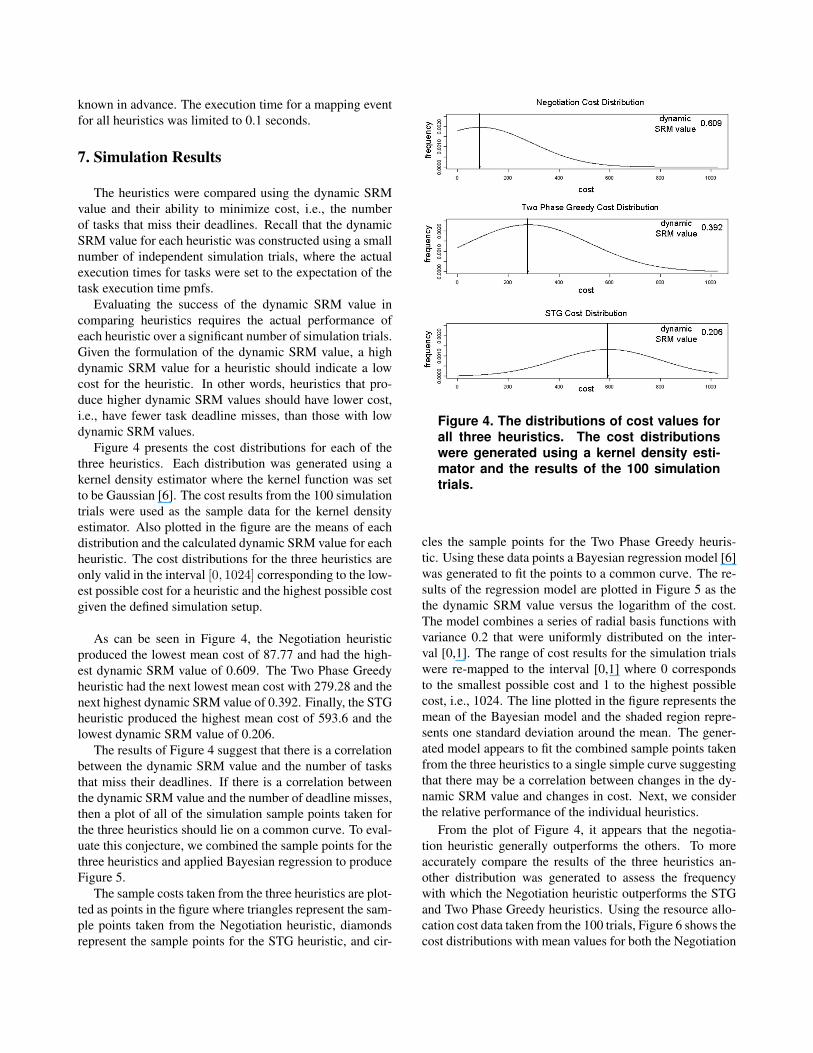
Figure 4 presents the cost distributions for each of thethree heuristics. Each distribution was generated using akernel density estimator where the kernel function was setto be Gaussian [6]. The cost results from the 100 simulationtrials were used as the sample data for the kernel densityestimator. Also plotted in the figure are the means of eachdistribution and the calculated dynamic SRM value for eachheuristic. The cost distributions for the three heuristics areonly valid in the interval [0, 1024] corresponding to the low-est possible cost for a heuristic and the highest possible costgiven the defined simulation setup.

As can be seen in Figure 4, the Negotiation heuristicproduced the lowest mean cost of 87.77 and had the high-est dynamic SRM value of 0.609. The Two Phase Greedyheuristic had the next lowest mean cost with 279.28 and thenext highest dynamic SRM value of 0.392. Finally, the STGheuristic produced the highest mean cost of 593.6 and thelowest dynamic SRM value of 0.206.

The results of Figure 4 suggest that there is a correlationbetween the dynamic SRM value and the number of tasksthat miss their deadlines. If there is a correlation betweenthe dynamic SRM value and the number of deadline misses,then a plot of all of the simulation sample points taken forthe three heuristics should lie on a common curve. To eval-uate this conjecture, we combined the sample points for thethree heuristics and applied Bayesian regression to produceFigure 5.

The sample costs taken from the three heuristics are plot-ted as points in the figure where triangles represent the sam-ple points taken from the Negotiation heuristic, diamondsrepresent the sample points for the STG heuristic, and cir-

Figure 4. The distributions of cost values forall three heuristics. The cost distributionswere generated using a kernel density esti-mator and the results of the 100 simulationtrials.

cles the sample points for the Two Phase Greedy heuris-tic. Using these data points a Bayesian regression model [6]was generated to fit the points to a common curve. The re-sults of the regression model are plotted in Figure 5 as thethe dynamic SRM value versus the logarithm of the cost.The model combines a series of radial basis functions withvariance 0.2 that were uniformly distributed on the inter-val [0,1]. The range of cost results for the simulation trialswere re-mapped to the interval [0,1] where 0 correspondsto the smallest possible cost and 1 to the highest possiblecost, i.e., 1024. The line plotted in the figure represents themean of the Bayesian model and the shaded region repre-sents one standard deviation around the mean. The gener-ated model appears to fit the combined sample points takenfrom the three heuristics to a single simple curve suggestingthat there may be a correlation between changes in the dy-namic SRM value and changes in cost. Next, we considerthe relative performance of the individual heuristics.

From the plot of Figure 4, it appears that the negotia-tion heuristic generally outperforms the others. To moreaccurately compare the results of the three heuristics an-other distribution was generated to assess the frequencywith which the Negotiation heuristic outperforms the STGand Two Phase Greedy heuristics. Using the resource allo-cation cost data taken from the 100 trials, Figure 6 shows thecost distributions with mean values for both the Negotiation

Figure 5. Plot of dynamic SRM value versus the logarithm of the costs for all three heuristics. ABayesian regression model has been used to fit a curve to the combined set of sample points for allthree heuristics. The line in the figure is the mean of the regression model and the shaded regionrepresents one standard deviation around the mean.

heuristic and the STG heuristic and a cost comparison forthe two. To generate the cost comparison distribution, la-beled “STG vs. Negotiation Cost Comparison,” the cost val-ues generated for the Negotiation heuristic were subtractedfrom those generated by the STG heuristic for each simula-tion trial. The samples used to define the actual executiontimes were drawn in advance of the simulation trials andwere the same for each heuristic. A kernel density estimatorwas then applied to the resultant data points to generate thedistributions in the figure. For each simulation trial, the Ne-gotiation heuristic produced a lower cost than that producedby the STG heuristic. However, for a small number of simu-lation trials the STG heuristic performed comparably to theNegotiation heuristic. These cost comparison values werevery close to zero but still slightly positive causing the tailof the cost comparison curve generated by the kernel den-sity estimator to edge into negative values. This suggeststhat there is a small probability that given the right circum-stances STG might perform better than Negotiation.

Figure 7 compares the cost distribution for the TwoPhase Greedy heuristic with the cost distribution for the Ne-gotiation heuristic. As can be seen in the comparison plot,labeled “Two Phase Greedy vs. Negotiation Cost Compar-

ison,” the density estimate of the comparison cost distribu-tion has a non-zero frequency for a sizable number of neg-ative values. That is, for these trials the Two Phase GreedyHeuristic had fewer task deadline misses than the Negoti-ation heuristic. However, for the majority of the trials theNegotiation heuristic outperformed the Two Phase Greedyheuristic. From the cost comparison plot this can be seenbecause the mean of the comparison cost distribution ispositive implying that more often than not the Two PhaseGreedy heuristic had a higher cost than Negotiation.

8. Related Work

In [14], the authors define a stochastic methodology forevaluating the robustness of a resource allocation in a sta-tic environment. In that work, uncertainty in system para-meters and its impact on system performance are modeledstochastically. This stochastic model was then used to de-rive a quantifiable measure of the robustness of a resourceallocation in a static environment. This was done by defin-ing stochastic completion times in a similar manner to our

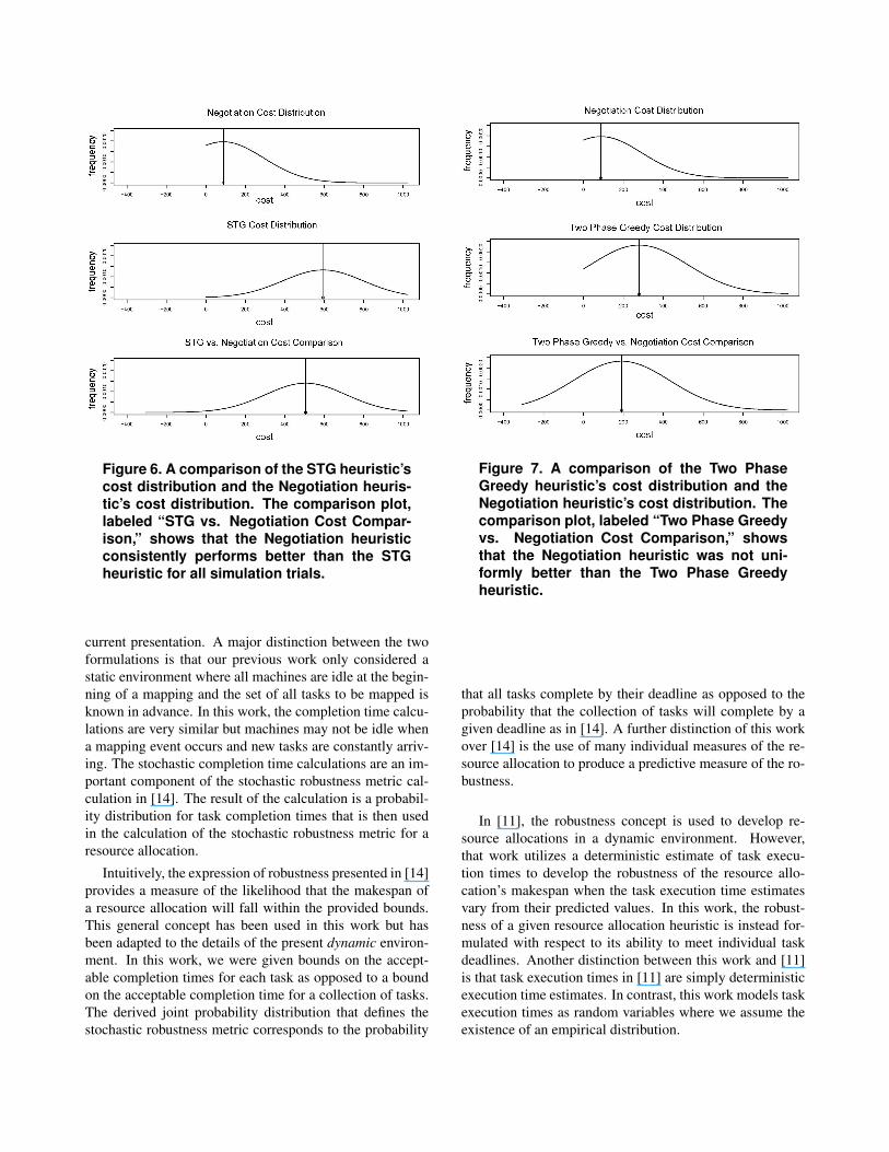
Figure 6. A comparison of the STG heuristic’scost distribution and the Negotiation heuris-tic’s cost distribution. The comparison plot,labeled “STG vs. Negotiation Cost Compar-ison,” shows that the Negotiation heuristicconsistently performs better than the STGheuristic for all simulation trials.

current presentation. A major distinction between the twoformulations is that our previous work only considered astatic environment where all machines are idle at the begin-ning of a mapping and the set of all tasks to be mapped isknown in advance. In this work, the completion time calcu-lations are very similar but machines may not be idle whena mapping event occurs and new tasks are constantly arriv-ing. The stochastic completion time calculations are an im-portant component of the stochastic robustness metric cal-culation in [14]. The result of the calculation is a probabil-ity distribution for task completion times that is then usedin the calculation of the stochastic robustness metric for aresource allocation.

Intuitively, the expression of robustness presented in [14]provides a measure of the likelihood that the makespan ofa resource allocation will fall within the provided bounds.This general concept has been used in this work but hasbeen adapted to the details of the present dynamic environ-ment. In this work, we were given bounds on the accept-able completion times for each task as opposed to a boundon the acceptable completion time for a collection of tasks.The derived joint probability distribution that defines thestochastic robustness metric corresponds to the probability

Figure 7. A comparison of the Two PhaseGreedy heuristic’s cost distribution and theNegotiation heuristic’s cost distribution. Thecomparison plot, labeled “Two Phase Greedyvs. Negotiation Cost Comparison,” showsthat the Negotiation heuristic was not uni-formly better than the Two Phase Greedyheuristic.

that all tasks complete by their deadline as opposed to theprobability that the collection of tasks will complete by agiven deadline as in [14]. A further distinction of this workover [14] is the use of many individual measures of the re-source allocation to produce a predictive measure of the ro-bustness.

In [11], the robustness concept is used to develop re-source allocations in a dynamic environment. However,that work utilizes a deterministic estimate of task execu-tion times to develop the robustness of the resource allo-cation’s makespan when the task execution time estimatesvary from their predicted values. In this work, the robust-ness of a given resource allocation heuristic is instead for-mulated with respect to its ability to meet individual taskdeadlines. Another distinction between this work and [11]is that task execution times in [11] are simply deterministicexecution time estimates. In contrast, this work models taskexecution times as random variables where we assume theexistence of an empirical distribution.

9. Conclusions

Our results suggest that there is an inverse relationshipbetween the dynamic SRM value and the performance ob-jective of the problem studied. In reviewing our results,we explored the general relationship between the dynamicSRM value and the performance objective by analyzing thefit of a Bayesian regression model to our results. The rel-atively good fit of the regression model to the combineddata of the three heuristics is strong evidence of the relation-ship between the dynamic SRM value and the stated perfor-mance objective. Our results appear to demonstrate that thedynamic SRM value can simplify the evaluation of resourceallocation heuristics in a dynamic environment. That is, themethodology for determining the dynamic SRM value fora heuristic reduces the number of simulations required todemonstrate the superiority of one heuristic over another ina dynamic resource allocation environment.

Using these results we compared the performance ofthree different heuristics taken from the literature and ap-plied to a stochastic dynamic environment. From this com-parison, the Negotiation heuristic showed promising resultsin this environment. Given the apparent relationship be-tween the dynamic SRM value and the stated performanceobjective, a valuable extension of this work would be the de-velopment of resource allocation heuristics that incorporatethe dynamic stochastic robustness metric during a resourceallocation.

References

[1] S. Ali, A. A. Maciejewski, H. J. Siegel, and J.-K. Kim. Mea-suring the robustness of a resource allocation. IEEE Trans-actions on Parallel and Distributed Systems, 15(7):630–641,July 2004.

[2] M. Arlitt and T. Jin. Workload characterization of the 1998world cup web site. Technical Report HPL-1999-35R1,Hewlett Packard Corporation, CA, Sept. 1999.

[3] M. Arlitt and T. Jin. A workload characterization study ofthe 1998 world cup web site. IEEE Network, 14:30–37,May/June 2000.

[4] L. Barbulescu, A. E. Howe, L. D. Whitley, and M. Roberts.Trading places: How to schedule more in a multi-resourceoversubscribed scheduling problem. In Proceedings ofthe International Conference on Automated Planning andScheduling (ICAPS 2004), pages 227–234, 2004.

[5] L. Barbulescu, L. D. Whitley, and A. E. Howe. Leap be-fore you look: An effective strategy in an oversubscribedscheduling problem. In Proceedings of the 19th NationalConference on Artifial Intelligence, pages 143–148, 2004.

[6] C. M. Bishop. Pattern Recognition and Machine Learning.Springer Science+Business Media, LLC, 233 Spring Street,New York, NY 10013, USA, first edition, 2006.

[7] T. D. Braun, H. J. Siegel, N. Beck, L. Boloni, R. F. Freund,D. Hensgen, M. Maheswaran, A. I. Reuther, J. P. Robert-

son, M. D. Theys, and B. Yao. A comparison of eleven sta-tic heuristics for mapping a class of independent tasks ontoheterogeneous distributed computing systems. Journal ofParallel and Distributed Computing, 61(6):810–837, June2001.

[8] O. H. Ibarra and C. E. Kim. Heuristic algorithms forscheduling independent tasks on non-identical processors.Journal of the ACM, 24(2):280–289, Apr. 1977.

[9] A. Leon-Garcia. Probability & Random Processes for Elec-trical Engineering. Addison Wesley, Reading, MA, 1989.

[10] M. Maheswaran, S. Ali, H. J. Siegel, D. Hensgen, and R. F.Freund. Dynamic mapping of a class of independent tasksonto heterogeneous computing systems. Journal of Paralleland Distributed Computing, 59(2):107–121, Nov. 1999.

[11] A. M. Mehta, J. Smith, H. J. Siegel, A. A. Maciejewski,A. Jayaseelan, and B. Ye. Dynamic resource allocationheuristics that manage tradeoff between makespan and ro-bustness. Journal of Supercomputing, Special Issue on GridTechnology, accepted, to appear.

[12] A. J. Page and T. J. Naughton. Dynamic task schedulingusing genetic algorithms for heterogeneous distributed com-puting. In Proceedings of the 19th International Paralleland Distributed Processing Symposium, Apr. 2005.

[13] K. Ross and N. Bambos. Local search scheduling algorithmsfor maximal throughput in packet switches. In Proceedingsof the 23rd Conference of the IEEE Communications Society(INFOCOM 2004), 2004.

[14] V. Shestak, J. Smith, H. J. Siegel, and A. A. Maciejewski. Astochastic approach to measuring the robustness of resourceallocations in distributed systems. In 2006 InternationalConference on Patallel Processing (ICPP 2006), pages 6–12, Aug. 2006.

[15] V. Shestak, J. Smith, R. Umland, J. Hale, P. Moranville,A. A. Maciejewski, and H. J. Siegel. Greedy approachesto static stochastic robust resource allocation for periodicsensor driven systems. In Proceedings of The 2006 Inter-national Conference on Parallel and Distributed Process-ing Techniques and Applications, volume 1, pages 3–9, June2006.

[16] R. Vaessens, E. Aarts, and J. Lenstra. Job-shopscheduling by local search. Technical Reporthttp://citeseer.ist.psu.edu/vaessens94job.html, EindhovenUniversity of Technology, Eindhoven, The Netherlands,1994 (accessed May 2006).

[17] L. Wasserman. All of Statistics: A Concise Course in Sta-tistical Inference. Springer Science+Business Media, NewYork, NY, 2005.

[18] M. Wu and W. Shu. Segmented min-min: A static mappingalgorithm for meta-tasks on heterogeneous computing sys-tems. In Proceedings of the 9th IEEE Heterogeneous Com-puting Workshop, pages 375–385, Mar. 2000.