Dual Stochastic Dominance and Quantile Risk Measures

Dual stochastic dominance and quantile risk measures

Włodzimierz Ogryczak and Andrzej Ruszczynskia

Warsaw University of Technology, Institute of Control and Computation Engineering, Nowowiejska 15/19,

00665 Warsaw, PolandaRutgers University, RUTCOR and Department of Management Science and Information Systems, Piscataway, NJ 08854,

USA

Received 18 June 2001; received in revised form 19 December 2001; accepted 23 January 2002

Abstract

Following the seminal work by Markowitz, the portfolio selection problem is usually modeled as a bicriteria

optimization problem where a reasonable trade-off between expected rate of return and risk is sought. In the

classical Markowitz model, the risk is measured with variance. Several other risk measures have been later

considered thus creating the entire family of mean-risk (Markowitz type) models. In this paper, we analyze

mean-risk models using quantiles and tail characteristics of the distribution. Value at risk (VAR), defined as the

maximum loss at a specified confidence level, is a widely used quantile risk measure. The corresponding second

order quantile measure, called the worst conditional expectation or Tail VAR, represents the mean shortfall at a

specified confidence level. It has more attractive theoretical properties and it leads to LP solvable portfolio

optimization models in the case of discrete random variables, i.e., in the case of returns defined by their

realizations under the specified scenarios. We show that the mean-risk models using the worst conditional

expectation or some of its extensions are in harmony with the stochastic dominance order. For this purpose, we

exploit duality relations of convex analysis to develop the quantile model of stochastic dominance for general

distributions.

Keywords: Portfolio optimization, stochastic dominance, mean-risk, value at risk, linear programming

1. Introduction

The relation of stochastic dominance is one of the fundamental concepts of decision theory (cf.

Whitmore and Findlay, 1978; Levy, 1992). It introduces a partial order in the space of real random

variables. The first-degree relation carries over to expectations of monotone utility functions, and the

second-degree relation to expectations of concave non-decreasing utility functions. While theoretically

attractive, stochastic dominance order is computationally very difficult, as a multi-objective model with

a continuum of objectives. Following the seminal work by Markowitz (1952), the portfolio optimization

problem is modeled as a mean-risk bicriteria optimization problem. The classical Markowitz model

Intl. Trans. in Op. Res. 9 (2002) 661–680

# 2002 International Federation of Operational Research Societies.

Published by Blackwell Publishers Ltd.

uses the variance as the risk measure. Since then many authors have pointed out that the mean–

variance model is, in general, not consistent with stochastic dominance rules.

When applied to portfolio selection or similar optimization problems with polyhedral feasible sets,

the mean-variance approach results in a quadratic programming problem. Following Sharpe’s (1971a)

work on linear programming (LP) approximation to the mean-variance model, many attempts have

been made to linearize the portfolio optimization problem. This resulted in the consideration of various

risk measures which were LP-computable in the case of finite discrete random variables. Yitzhaki

(1982) introduced the mean-risk model using the Gini’s mean (absolute) difference as a risk measure.

Konno and Yamazaki (1991) analyzed the model where risk is measured by the (mean) absolute

deviation. Young (1998) considered the minimax approach (the worst-case performances) to measure

the risk. If the rates of return are multivariate normally distributed, then most of these models are

equivalent to the Markowitz’ mean-variance model. However, they do not require any specific type of

return distributions and, opposite to the mean-variance approach, they can be applied to general

(possibly non-symmetric) random variables (Michalowski and Ogryczak, 2001). In the case of finite

discrete random variables all these mean-risk models have LP formulations and are special cases of the

multiple criteria LP model (Ogryczak, 2000) based on the majorization theory (Marshall and Olkin,

1979) and Lorenz-type orders (Shorrocks, 1983).

In this paper, we analyze mean-risk models using quantiles and tail characteristics of the distribution.

Value at risk (VAR), defined as the maximum loss at a specified confidence level, is a widely-used

quantile risk measure (Jorion, 1997). The corresponding second order quantile measure, called the

worst conditional expectation or Tail VAR, represents the mean shortfall at a specified confidence level.

It leads to LP-solvable portfolio optimization models in the case of discrete random variables, i.e., in

the case of returns defined by their realizations under the specified scenarios. The worst conditional

expectation itself and some of its extensions have attractive theoretical properties. We show that the

corresponding mean-risk models are in harmony with the stochastic dominance order. For this purpose,

we exploit duality relations of convex analysis to develop the dual (quantile) model of the stochastic

dominance for general distributions. The only restriction we impose is that all the random returns R

under consideration satisfy the condition EjRj , 1. The results are graphically illustrated within the

framework of the absolute Lorenz curves (dual SSD) as well as the Outcome–Risk diagram (primal

SSD).

The paper is organized as follows. In Section 2 we formally define the concepts of consistency of the

mean-risk models with the stochastic dominance relations. Section 3 introduces primal and dual

shortfall risk measures and exploits the duality theory to characterize the stochastic dominance

relations in terms of quantile performance funtions. This allows us to relate the quantile risk measures

with the stochastic dominance. In Section 4, the LP solvability of the corresponding mean-risk models

is discussed, and some extensions are considered.

2. Stochastic dominance and mean-risk models

The portfolio optimization problem considered in this paper is based on a single-period model of

investment. Let J ¼ f1, 2, . . ., ng denote a set of securities considered for an investment. For each

security j 2 J, its rate of return is represented by a random variable Rj with a given mean � j ¼ EfRjg.

Further, let x ¼ (xj) j¼1,..., n denote a vector of decision variables xj expressing the weights defining a

662 W. Ogryczak and A. Ruszczynski / Intl. Trans. in Op. Res. 9 (2002) 661–680

portfolio. To represent a portfolio, the weights must satisfy a set of constraints that form a feasible set

P . The simplest way of defining a feasible set is by a requirement that the weights must sum to one,

i.e.Pn

j¼1xj ¼ 1 and xj > 0 for j ¼ 1, . . ., n. An investor usually needs to consider some other

requirements expressed as a set of additional side constraints. Hereafter, it is assumed that P is a

general LP-feasible set given in a canonical form as a system of linear equations with non-negative

variables.

Each portfolio x defines a corresponding random variable R(x) ¼Pn

j¼1 Rjxj that represents a

portfolio return. The mean return for portfolio x is given as �(x) ¼ EfR(x)g ¼Pn

j¼1� jxj. Following

Markowitz (1952), the portfolio optimization problem is modeled as a mean-risk bicriteria optimization

problem

maxf[�(x), �æ(x)]: x 2 P g (1)

where the mean �(x) is maximized and the risk measure æ(x) is minimized. A feasible portfolio

x0 2 P is called the efficient solution of problem (1) or the �=æ–efficient portfolio if there is no x 2 P

such that �(x) > �(x0) and æ(x) < æ(x0) with at least one inequality strict. We restrict our analysis to

the class of Markowitz-type mean-risk models where risk measures, similar to the standard deviation,

are translation invariant and risk relevant dispersion parameters. Thus the risk measures we consider

are not affected by any shift of the outcome scale and they are equal to 0 in the case of a risk-free

portfolio, while taking positive values for any risky portfolio. Moreover, in order to model possible

taking advantages of a portfolio diversification, risk measure æ(x) should be a convex function of x.

The Markowitz model is frequently criticized as not consistent with axiomatic models of preferences

for choice under risk. Namely, except for the case of returns meeting the multivariate normal

distribution, the mean-variance model may lead to inferior conclusions with respect to the stochastic

dominance order. The concept of stochastic dominance order (Whitmore and Findlay, 1978) corre-

sponds to an expected utility axiomatic model of risk-averse preferences (Rothschild and Stiglitz,

1969; Levy, 1992). In stochastic dominance, uncertain returns (random variables) are compared by

pointwise comparison of some performance functions constructed from their distribution functions.

The first performance function F (1) is defined as the right-continuous cumulative distribution function:

F(1)R (�) ¼ FR(�) ¼ PfR < �g. The weak relation of the first degree stochastic dominance (FSD) is

defined as follows:

R9 � FSD R 0 , FR9(�) < FR 0(�) for all �:

The second function is derived from the first as F(2)R (�) ¼

Ð ��1 FR(�)d� for real numbers �, and it

defines the (weak) relation of second degree stochastic dominance (SSD):

R9 � SSD R 0 , F(2)R9 (�) < F

(2)R 0(�) for all �:

We say that portfolio x9 dominates x 0 under the SSD (R(x9) SSD R(x 0 )), if F(2)R(x9)(�) < F

(2)R(x 0 )(�) for

all �, with at least one strict inequality. A feasible portfolio x0 2 P is called SSD efficient if there is no

x 2 P such that R(x) SSD R(x0). If R(x9) SSD R(x 0 ), then R(x9) is preferred to R(x 0 ) within all

risk-averse preference models where larger outcomes are preferred. It is therefore a matter of primary

importance that a model for portfolio optimization be consistent with the SSD relation, which implies

that the optimal portfolio is SSD-efficient.

The Markowitz model is not SSD consistent, since its efficient set may contain portfolios

characterized by a small risk, but also very low return (Porter and Gaumnitz, 1972). Unfortunately, it is

W. Ogryczak and A. Ruszczynski / Intl. Trans. in Op. Res. 9 (2002) 661–680 663

a common flaw of all Markowitz-type mean-risk models where risk is measured with some dispersion

measures. Although, the necessary condition for the SSD relation is (Fishburn, 1980)

R(x9) � SSD R(x 0 ) ) �(x9) > �(x 0 ) (2)

this is not enough to guarantee the �=æ dominance. For dispersion-type risk measures æ(x), it may

occur that R(x9) SSD R(x 0 ) and simultaneously æ(x9) . æ(x 0 ). This can be illustrated by two

portfolios x9 and x 0 with returns given as follows:

PfR(x9) ¼ �g ¼ 1 � ¼ 1:00, otherwise

�PfR(x 0 ) ¼ �g ¼

1=2, � ¼ 3:01=2, � ¼ 5:00, otherwise

8<:

Note that the risk-free portfolio x9 with the guaranteed result 1.0 is obviously worse than the risky

portfolio x 0 giving 3.0 or 5.0. In all preference models based on the risk aversion axioms (Artzner et

al., 1999; Levy, 1992; Whitmore and Findlay, 1978) portfolio x9 is dominated by x 0, in particular

R(x 0 ) SSD R(x9). On the other hand, when a dispersion-type risk measure æ(x) is used, then both the

portfolios are efficient in the corresponding mean-risk model since for each such a measure æ(x 0 ) . 0

while æ(x9) ¼ 0.

In order to overcome this flaw of the Markowitz model, Baumol (1964) suggested a safety measure

he called the expected gain-confidence limit criterion, �(x) � º� (x) to be maximized instead of the

minimization of � (x) itself. Similarly, Yitzhaki (1982) considered maximization of the safety measure

�(x) � ˆ(x) defined by the risk measure of Gini’s mean difference ˆ(x), and he demonstrated its SSD

consistency. Markowitz (1959) introduced two downside risk measures to replace the variance: the

below-target downside semivariance and the below-mean downside semivariance. For the former, its

SSD consistency was shown by Porter (1994). Recently, similar consistency results have been

introduced (Ogryczak and Ruszczynski, 1999, 2001) for safety measures corresponding to the below-

mean downside standard semideviation and to the below-mean downside mean semideviation (half of

the mean absolute deviation). Hereafter, for any dispersion type risk measure æ(x), the function

s(x) ¼ �(x) � æ(x) will be referred to as the corresponding safety measure. Note that risk measures, we

consider, are defined as translation-invariant and risk-relevant dispersion parameters. Hence, the

corresponding safety measures are translation equivariant in the sense that any shift of the outcome

scale results in an equivalent change of the safety measure value (with opposite sign as safety measures

are maximized). In other words, the safety measures distinguish (and order) various risk-free portfolios

(outcomes) according to their values. The safety measures, we consider, are risk relevant, but in the

sense that the value of a safety measure for any risky portfolio is less than the value for the risk-free

portfolio with the same expected return. Moreover, when risk measure æ(x) is a convex function of x,

then the corresponding safety measure s(x) is concave.

The SSD consistency of the safety measures may be formalized as follows. We say that the safety

measure �(x) � æ(x) is SSD consistent or that the risk measure æ(x) is SSD safety consistent if

R(x9) � SSD R(x 0 ) ) �(x9) � æ(x9) > �(x 0 ) � æ(x 0 ) (3)

The relation of SSD (safety) consistency is called strong if, in addition to (3), the following holds

R(x9) SSD R(x 0 ) ) �(x9) � æ(x9) . �(x 0 ) � æ(x 0 ) (4)


Theorem 1. If the risk measure æ(x) is SSD safety consistent (3), then except for portfolios with

identical values of �(x) and æ(x), every efficient solution of the bicriteria problem

maxf[�(x), �(x) � æ(x)]: x 2 P g (5)

is an SSD efficient portfolio. In the case of strong SSD safety consistency (4), every portfolio x 2 P

efficient to (5) is, unconditionally, SSD efficient.

Proof. Let x0 2 P be an efficient solution of (5). Suppose that x0 is not SSD efficient. This means,

there exists x 2 P such that R(x) SSD R(x0). Then, from (2) it follows �(x) > �(x0), and simulta-

neously �(x) � æ(x) > �(x0) � æ(x0), by virtue of the SSD safety consistency (3). Since x0 is efficient

to (5) no inequality can be strict, which implies �(x) ¼ �(x0) and æ(x) ¼ æ(x0).

In the case of the strong SSD safety consistency (4), the supposition R(x) SSD R(x0) implies

�(x) > �(x0) and �(x) � æ(x) . �(x0) � æ(x0) which contradicts the efficiency of x0 with respect to

(5). Hence, x0 is SSD efficient.

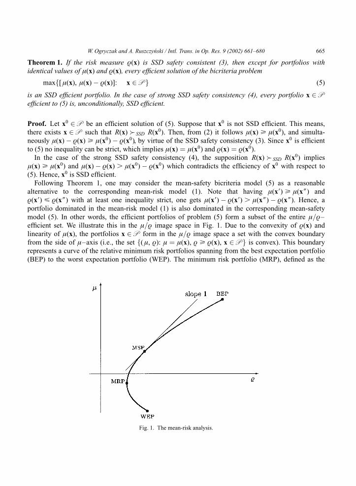
Following Theorem 1, one may consider the mean-safety bicriteria model (5) as a reasonable

alternative to the corresponding mean-risk model (1). Note that having �(x9) > �(x 0 ) and

æ(x9) < æ(x 0 ) with at least one inequality strict, one gets �(x9) � æ(x9) . �(x 0 ) � æ(x 0 ). Hence, a

portfolio dominated in the mean-risk model (1) is also dominated in the corresponding mean-safety

model (5). In other words, the efficient portfolios of problem (5) form a subset of the entire �=æ–

efficient set. We illustrate this in the �=æ image space in Fig. 1. Due to the convexity of æ(x) and

linearity of �(x), the portfolios x 2 P form in the �=æ image space a set with the convex boundary

from the side of �–axis (i.e., the set f(�, æ): � ¼ �(x), æ > æ(x), x 2 P g is convex). This boundary

represents a curve of the relative minimum risk portfolios spanning from the best expectation portfolio

(BEP) to the worst expectation portfolio (WEP). The minimum risk portfolio (MRP), defined as the

Fig. 1. The mean-risk analysis.


solution of minx2P æ(x), limits the curve to the mean-risk efficient frontier from BEP to MRP. Similar,

the maximum safety portfolio (MSP), defined as the solution of maxx2P [�(x) � æ(x)], distinguishes a

part of the mean-risk efficient frontier, from BEP to MSP, which is also mean-safety efficient. By virtue

of Theorem 1, in the case of an SSD safety consistent risk measure, this part of the efficient frontier

represents portfolios which are SSD efficient. Exactly, if a point (�, æ) located at the efficient frontier

between BEP and MSP is generated by the unique portfolio, then this portfolio is SSD efficient. In the

case of multiple portfolios generating the same point (�, æ), at least one of them is SSD efficient, but

some other portfolios may be SSD dominated (by that efficient). The strong SSD consistency

guarantees that all possible alternative portfolios are SSD efficient.

For specific types of return distributions or specific feasible sets, the subset of portfolios with

guaranteed SSD efficiency may be larger (Ogryczak and Ruszczynski, 1999), exceeding the limit of

the MSP. Hence, the mean-safety model (5) may be too restrictive in some practical investment

decisions and it may be important to keep the full modeling capabilities of the original mean-risk

approach (1). On the other hand, some mean-risk models, like the minimax (Young, 1998), were

originally introduced in the form of corresponding mean-safety models (5). Therefore, the only way to

provide a platform for the analysis of various Markowitz-type models is, in our opinion, to consider

both mean-risk and mean-safety forms for all the measures.

An implementation of the Markowitz-type mean-risk model may take advantage of the efficient

frontier convexity to perform the trade-off analysis. Having assumed a trade-off coefficient º between

the risk and the mean, the so-called risk aversion coefficient, one may directly compare real values

�(x) � ºæ(x) and find the best portfolio by solving the optimization problem:

maxf�(x) � ºæ(x): x 2 P g: (6)

Various positive values of parameter º allow us to generate various efficient portfolios. By solving a

parametric problem equation (6) with changing º . 0 one gets the so-called critical line approach

(Markowitz, 1959). Due to convexity of risk measures æ(x) with respect to x, º . 0 provides a

parameterization of the entire set of the �=æ–efficient portfolios (except of its two ends BEP and MRP

which are the limiting cases). Note that (1 � º)�(x) þ º(�(x) � æ(x)) ¼ �(x) � ºæ(x). Hence, bounded

trade-off 0 , º , 1 in the Markowitz-type mean-risk model (1) corresponds to the complete weighting

parameterization of the mean-safety model (5). This allows us to use Theorem 1 to derive the following

SSD consistency results for the trade-off approach.

Corollary 1. If the risk measure æ(x) is SSD safety consistent (3), then except for portfolios with

identical values of �(x) and æ(x), every optimal solution of problem (6) with 0 , º , 1 is an SSD

efficient portfolio. In the case of strong SSD safety consistency (4), every portfolio x 2 P optimal to

(6) with 0 , º , 1 is, unconditionally, SSD efficient.

Recall that for specific types of return distributions or specific feasible sets the subset of portfolios

with guaranteed SSD efficiency may be larger and this can easily be represented by the larger upper

limit on º. For instance, in the case of risk measures defined as the mean semideviation or the Gini’s

mean difference, this upper limit may be doubled still guaranteeing the SSD efficiency for solutions

with 0 , º , 2, provided that the return distributions are symmetric with respect to their means

(Ogryczak and Ruszczynski, 1999, 2002). Thus the trade-off model (6) offers a universal tool covering


both the standard mean-risk and the corresponding mean-safety approaches. It provides easy modeling

of the risk aversion and control of the SSD efficiency.

3. Dual stochastic dominance and shortfall risk measures

The notion of risk is related to a possible failure of achieving some targets and was formalized as the

so-called shortfall criteria. The simplest shortfall criterion for a target value � is the probability of

underachievement PfR < �g, which is used in the FSD relation. Function F (2), used to define the SSD

relation, can be presented as follows (Ogryczak and Ruszczynski, 1999):

F(2)R (�) ¼ PfR < �gEf�� RjR < �g ¼ Efmaxf�� R, 0gg:

Hence, the SSD relation is the Pareto dominance for mean below-target deviations from infinite

number (continuum) of targets. The function F(2)R is well-defined for any random variable R satisfying

the condition EjRj , 1. As shown by Ogryczak and Ruszczynski (1999), it is a continuous, convex,

non-negative, and non-decreasing function of �. The graph F(2)R(x)(�), referred to as the Outcome–Risk

(O–R) diagram, has two asymptotes which intersect at the point (�(x), 0). Specifically, the �-axis is

the left asymptote and the line �� (x) is the right asymptote (Fig. 2). In the case of a deterministic

(risk-free) return (R(x) ¼ �(x)), the graph of F(2)R(x)(�) coincides with the asymptotes, whereas any

uncertain return with the same expected value �(x) yields a graph above (precisely, not below) the

asymptotes. The space between the curve (�, F(2)R(x)(�)), and its asymptotes represents the dispersion

(and thereby the riskiness) of R(x) in comparison to the deterministic return �(x). Therefore, it is called

the dispersion space. While the variance � 2(x) represents the doubled area of the dispersion space, the

mean semideviation (from the mean) �(x) ¼ Efmaxf�(x) � R(x), 0gg ¼ F(2)R(x)(�(x)) turns out to be

its largest vertical diameter. Therefore (Ogryczak and Ruszczynski, 1999), the mean semideviation is

SSD safety consistent, i.e., R(x9) � SSD R(x 0 ) implies �(x9) � �(x9) > �(x 0 ) � �(x 0 ). The mean

semideviation is a half of the mean absolute deviation �(x) ¼ Efj�(x) � R(x)jg ¼ 2�(x). Hence, the

corresponding mean-risk model is equivalent to the MAD model (Konno and Yamazaki, 1991).

The mean below-target deviation from a specific target represents a single criterion of the SSD

Fig. 2. The O–R diagram.


relation. Such a shortfall measure is very useful in investment situations with clearly defined minimum

acceptable returns (e.g. bankruptcy level). However, in general cases, the quantile shortfall risk

measures are more commonly used and accepted. In banking it was formalized with the Basle

Committee on Banking Supervision recommending the measure of value at risk (VAR) defined as the

maximum loss at a specified confidence level (c.f. Jorion, 1997; and references therein). VAR is now a

widely used quantile measure, although the VAR calculations are usually based on the normal

distribution assumption (Morgan, 1996). In this paper we do consider VAR measures for arbitrary

distribution, following the original definition of the VAR as a high quantile (typically 95th or 99th

percentile) of a distribution of losses.

Given p 2 [0, 1], the number qR( p) is called a p-quantile of the random variable R if

PfR , qR( p)g < p < PfR < qR( p)g:For p 2 (0, 1) the set of such p-quantiles is a closed interval (Embrechts, Kluppelberg and Mikosch,

1997). Recall that value at risk depicts the worst (maximum) loss within a given confidence interval

(Jorion, 1997). Hence, for a given portfolio x generating random returns R(x) its value at risk for a

confidence level c is a c-quantile of the random variable �R(x), where the minus sign is due to

counting losses while R(x) represents the portfolio returns. In order to formalize the quantile measures,

we introduce the first quantile function F(�1)R corresponding to a real random variable R as the left-

continuous inverse of the cumulative distribution function FR:

F(�1)R ( p) ¼ inf f� : FR(�) > pg for 0 , p < 1:

The value F(�1)R ( p) represents the p-quantile of R and, in the case of a non-unique quantile, it is the left

end of the entire interval of quantiles. For a given portfolio x, its VAR for a confidence level c may

now be written as

VARc(x) ¼ supf� : Pf�R(x) , �g < cg

¼ �inff� : PfR(x) < �g > 1 � cg ¼ �F(�1)R(x)(1 � c): (7)

The above formula defines the so-called absolute VAR related to the absolute loss. One may also

consider the loss relative to the mean return (Jorion, 1997) which results in the following formula

RVARc(x) ¼ �(x) � F(�1)R(x)(1 � c). Note that VARc(x) ¼ RVARc(x) � �(x). In the case of a risk-

free portfolio R(x) ¼ �(x), for any confidence level 0 , c , 1 one has RVARc(x) ¼ 0 and

VARc(x) ¼ ��(x). Hence, in terms of the Markowitz-type mean-risk analysis, we consider, the relative

value at risk is the risk measure RVARc(x) ¼ æ(x) while the absolute VAR is the negative of the

corresponding safety measure VARc(x) ¼ æ(x) � �(x) ¼ �s(x).

Directly from the definition of FSD we see that

R9 � FSD R 0 , F(�1)R9 ( p) > F

(�1)R 0 ( p) for all 0 , p < 1:

Thus, the function F (�1) can be considered as a continuum-dimensional safety measure within the

FSD. Using any specific (left) quantile as a scalar safety measure is consistent with the FSD. This

justifies VARc(x) for any 0 < c , 1, when minimized, as an FSD-consistent measure in the sense that

R(x9) � FSD R(x 0 ) implies VARc(x9) < VARc(x 0 ). This does not guarantee, however, any consistency

with the SSD, because it may happen that R9 � SSD R 0, but F(�1)R9 ( p) , F

(�1)R 0 ( p) for some p. The lack

of the SSD consistency we illustrate by two portfolios x9 and x 0 with returns given as follows:


PfR(x9) ¼ �g ¼

0:01, � ¼ �10

0:05, � ¼ �6

0:94, � ¼ 10

0, otherwise

8>><>>: PfR(x 0 ) ¼ �g ¼

0:03, � ¼ �10

0:05, � ¼ �4

0:90, � ¼ 10

0:02, � ¼ 25

0, otherwise

8>>>><>>>>:

(8)

Note that �(x9) ¼ �(x 0 ) ¼ 9 and � (x9) , � (x 0 ) as well as �(x9) , �(x 0 ). Actually, R(x9) SSD R(x 0 )

and in all preference models based on the risk-aversion axioms portfolio x9 is preferred to x 0. On the

other hand, when calculating the VAR measures for the 95% confidence level one gets VAR:95(x9) ¼ 6

and RVAR:95(x9) ¼ 15 while VAR:95(x 0 ) ¼ 4 and RVAR:95(x 0 ) ¼ 13. Thus, portfolio x9 is considered

as more risky with respect to both the absolute and the relative VAR measures. There are also known

examples showing directly that increasing diversification of a portfolio results in the larger value of the

VAR measure (Artzner et al., 1999).

To obtain quantile measures consistent with the SSD we introduce the second quantile function

defined for a random variable R as:

F(�2)R ( p) ¼

ð p

0

F(�1)R (Æ)dÆ for 0 , p < 1 and F

(�2)R (0) ¼ 0: (9)

Similarly to F(2)R , the function F

(�2)R is well-defined for any random variable R satisfying the condition

E jRj , 1. By construction, it is convex. The graph of F(�2)R is called the absolute Lorenz curve or

ALC diagram for short. The pointwise comparison of the second quantile functions defines the so-

called absolute (or general) Lorenz order (Shorrocks, 1983).

Recently, an intriguing duality relation between the second quantile function F(�2)R and the second

performance function F(2)R

has been shown (Ogryczak and Ruszczynski, 2002). Namely, function F(�2)R

is a conjugent (dual function) (Rockafellar, 1970) of F(2)R , i.e., for every p 2 [0, 1],

F(�2)R ( p) ¼ sup

�f� p � F

(2)R (�)g: (10)

It follows from the duality theory (Rockafellar, 1970) that we may fully characterize the SSD relation

by using the conjugate function F (�2):

R9 � SSD R 0 , F(�2)R9 ( p) > F

(�2)R 0 ( p) for all 0 < p < 1: (11)

In other words, the absolute Lorenz order is equivalent to the SSD order.

By the properties of the O–R diagram and equation (10), for any portfolio x one gets

F(�2)R(x)

(1) ¼ �(x). Thus the ALC diagram is a continuous convex curve connecting points (0, 0) and

(1, �(x)), whereas a deterministic outcome with the same expected value �(x), yields the chord

(straight line) connecting the same points. Hence, the space between the curve ( p, F(�2)R(x)( p)),

0 < p < 1, and its chord represents the dispersion (and thereby the riskiness) of R(x) in comparison to

the deterministic outcome of �(x) (Fig. 3). We shall call it the dual dispersion space. Both size and

shape of the dual dispersion space are important for complete description of the riskiness of a portfolio.

Nevertheless, it is quite natural to consider some size parameters as summary characteristics of

riskiness.


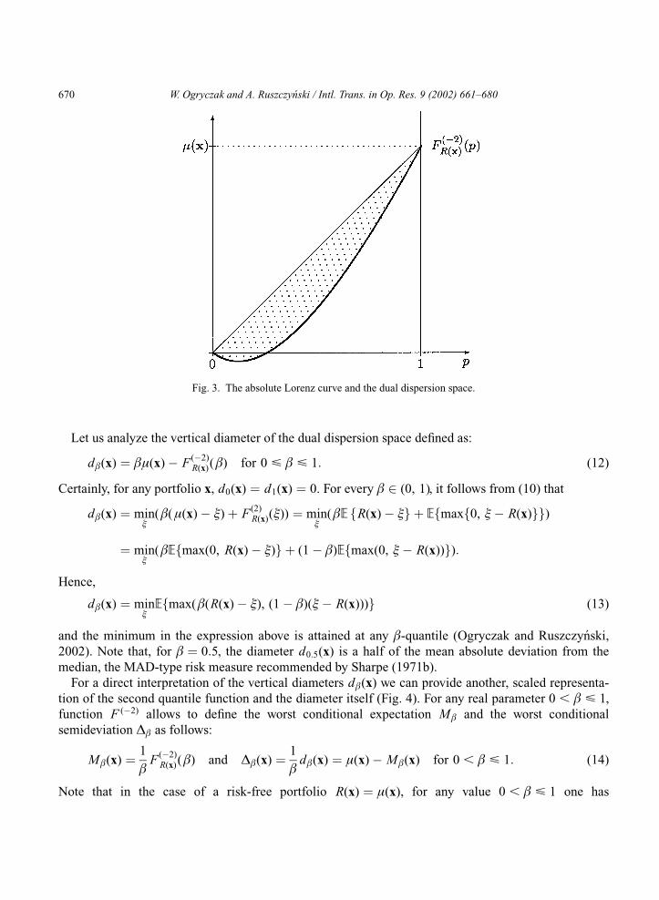
Let us analyze the vertical diameter of the dual dispersion space defined as:

d(x) ¼ �(x) � F(�2)R(x)() for 0 < < 1: (12)

Certainly, for any portfolio x, d0(x) ¼ d1(x) ¼ 0. For every 2 (0, 1), it follows from (10) that

d(x) ¼ min�

((�(x) � �) þ F(2)R(x)(�)) ¼ min

�(E fR(x) � �g þ Efmaxf0, �� R(x)gg)

¼ min�

(Efmax(0, R(x) � �)g þ (1 � )Efmax(0, �� R(x))g):

Hence,

d(x) ¼ min�Efmax((R(x) � �), (1 � )(�� R(x)))g (13)

and the minimum in the expression above is attained at any -quantile (Ogryczak and Ruszczynski,

2002). Note that, for ¼ 0:5, the diameter d0:5(x) is a half of the mean absolute deviation from the

median, the MAD-type risk measure recommended by Sharpe (1971b).

For a direct interpretation of the vertical diameters d(x) we can provide another, scaled representa-

tion of the second quantile function and the diameter itself (Fig. 4). For any real parameter 0 , < 1,

function F (�2) allows to define the worst conditional expectation M and the worst conditional

semideviation ˜ as follows:

M(x) ¼ 1

F

(�2)R(x)() and ˜(x) ¼ 1

d(x) ¼ �(x) � M(x) for 0 , < 1: (14)

Note that in the case of a risk-free portfolio R(x) ¼ �(x), for any value 0 , < 1 one has

Fig. 3. The absolute Lorenz curve and the dual dispersion space.


M(x) ¼ �(x) and ˜(x) ¼ 0. Hence, in terms of the Markowitz-type mean-risk analysis, we consider,

the worst conditional semideviation is the risk measure ˜(x) ¼ æ(x), while the worst conditional

expectation itself is the corresponding safety measure M(x) ¼ �(x) � æ(x) ¼ s(x). By the convexity

of F (�2), the worst conditional expectation M(x) is non-decreasing and continuous function of . Note

that M1(x) ¼ �(x) and ˜1(x) ¼ 0. In the case of a random variable with lower bounded support, the

value of M(x) tends to the minimum outcome M(x) when approaches 0 ( ! 0þ). Hence, the

minimax portfolio selection rule of Young (1998) is a limiting case of the mean-risk model using the

worst conditional expectation.

The relation (11) can be rewritten in the form

R9 � SSD R 0 , F(�2)R9 ( p)=p > F

(�2)R 0 ( p)=p for all 0 , p < 1, (15)

thus justifying the SSD consistency of the worst conditional expectation M(x) as a safety measure.

Proposition 1. For any 0 , < 1, the worst conditional semideviation ˜(x) is an SSD safety

consistent risk measure, in the sense that

R(x9) � SSD R(x 0 ) ) M(x9) ¼ �(x9) � ˜(x9) > M(x 0 ) ¼ �(x 0 ) � ˜(x 0 ): (16)

Let p 2 (0, 1) and suppose that � is such that PfR(x) < �g ¼ p. Then, by the theory of conjugate

functions (Rockafellar, 1970, Thm.23.5), the equality F(�2)R(x)( p) þ F

(2)R(x)(�) ¼ p� holds.

Fig. 4. The absolute Lorenz curve and the conditional worst realizations.


Hence, in the case of PfR(x) < �VARc(x)g ¼ 1 � c, one gets

M (1�c)(x) ¼ �VARc(x) � 1

1 � cF

(2)R(x)(�VARc(x))

¼ �VARc(x) þ EfR(x) þ VARc(x)jR(x) < �VARc(x)g

¼ EfR(x)jR(x) < �VARc(x)g:

Hence, the quantity M (1�c)(x) may be interpreted as the negative to the expected loss size, given that

the losses on the level of VARc(x) or greater are considered. The latter is called the expected shortfall

ESc(x) ¼ Ef�R(x)j � R(x) > VARc(x)g (Embrechts et al., 1997), the Tail Conditional Expectation

(Tail VAR) (Artzner et al., 1999) or the conditional value at risk (CVAR) (Andersson et al., 2001).

Similar characteristics called absolute concentration curves were earlier considered by Shalit and

Yitzhaki (1994). They compared absolute concentration curves for individual securities Rj in their

analysis if there are securities whose share will be increased by every risk-averse investor. The relation

M (1�c)(x) ¼ �Ef�R(x)j � R(x) > VARc(x)g ¼ �ESc(x) (17)

facilitates the understanding of the measure of the worst conditional expectation (Artzner et al., 1999)

and the nature of the second quantile function (Shalit and Yitzhaki, 1994). Although valid for many

continuous distributions (Andersson et al., 2001) equation (17), in general, cannot serve as a definition

of the worst conditional expectation because � such that PfR(x) < �g ¼ p need not exist.

In general, PfR(x) < �VARc(x)g ¼ 9 > ¼ 1 � c and M(x) < M9(x) ¼ EfR(x)jR(x) <

�VARc(x)g. Moreover, while according to Proposition 1 the worst conditional expectation is always

SSD consistent, this is not true for the expected shortfall (or equivalent measures). We illustrate this

by two portfolios x9 and x 0 with returns given in (8). Recall that �(x9) ¼ �(x 0 ) ¼ 9 and

R(x9) SSD R(x0 ). When calculating the VAR measures for the 95% confidence level we got

VAR:95(x9) ¼ 6 and VAR:95(x 0 ) ¼ 4. Now, computing the worst conditional expectations we get

M :05(x9) ¼ (�10 . 0:01 � 6 . 0:04)=0:05 ¼ �6:8 . M :05(x 0 ) ¼ (�10 . 0:03 � 4 . 0:02)=0:05 ¼ �7:6,

thus preferring portfolio x9 as less risky. On the other hand, when calculating the expected shortfalls for

the 95% confidence level, one gets

ES:95(x9) ¼ (10 . 0:01 þ 6 . 0:05)=0:06 ¼ 40=6 . ES:95(x 0 ) ¼ (10 . 0:03 þ 4 . 0:05)=0:08 ¼ 6:26:

Thus, despite R(x9) SSD R(x0 ), the portfolio x9 would be considered as more risky with respect to the

expected shortfall measures.

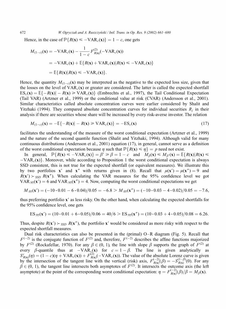
Dual risk characteristics can also be presented in the (primal) O–R diagram (Fig. 5). Recall that

F (�2) is the conjugate function of F (2) and, therefore, F (�2) describes the affine functions majorized

by F (2) (Rockafellar, 1970). For any 2 (0, 1), the line with slope supports the graph of F (2) at

every -quantile thus at �VARc(x) for c ¼ 1 � . The line is given analytically as

ScR(x)(�) ¼ (1 � c)(�þ VARc(x)) þ F

(2)R(x)(�VARc(x)). The value of the absolute Lorenz curve is given

by the intersection of the tangent line with the vertical (risk) axis, F(�2)R(x)() ¼ �S

(1�)R(x) (0). For any

2 (0, 1), the tangent line intersects both asymptotes of F (2). It intersects the outcome axis (the left

asymptote) at the point of the corresponding worst conditional expectation: � ¼ F(�2)R(x)()= ¼ M(x).


4. LP computability

While the original Markowitz model with risk measured by the variance forms a quadratic program-

ming problem, following Sharpe (1971a), many attempts have been made to linearize the portfolio

optimization procedure (c.f., Speranza, 1993, and references therein). Certainly, to model advantages

of a diversification, risk measures cannot be a linear function of x. Nevertheless, the risk measure can

be LP-computable in the case of discrete random variables, i.e., in the case of returns defined by their

realizations under the specified scenarios. We will consider T scenarios with probabilities pt (where

t ¼ 1, . . ., T). We will assume that for each random variable Rj there is known its realization r jt under

the scenario t. Typically, the realizations are derived from historical data treating T historical periods

as equally probable scenarios ( pt ¼ 1=t). The realizations of the portfolio returns R(x) are given as

yt ¼Pn

j¼1 r jtxj and the expected value can be computed as �(x) ¼PT

t¼1 yt pt ¼PT

t¼1[ pt

Pnj¼1 r jtxj].

Several risk measures can be LP-computable with respect to the realizations yt. Konno and Yamazaki

(1991) presented and analyzed the complete portfolio optimization model (MAD model) based on the

risk measure defined as the mean absolute deviation from the mean �(x) ¼ EfjR(x) � �(x)jg. For a

discrete random variable represented by its realizations yt, the mean absolute deviation, when

minimized, is LP-computable as

�(x) ¼ minXT

t¼1

(d�t þ dþ

t ) pt s:t: d�t � dþ

t ¼ �(x) � yt, d�t , dþ

t > 0 for t ¼ 1, . . ., T (18)

where d�t and dþ

t are nonnegative variables introduced to represent, respectively, the downside and the

upside deviation from the mean return under the scenario t. This can be simplified by taking advantages

of the symmetry �(x) ¼ 2�(x) as

Fig. 5. Quantile safety measures in the O–R diagram.


�(x) ¼ minXT

t¼1

d�t pt s:t: d�

t > �(x) � yt, d�t > 0 for t ¼ 1, . . ., T :

Yitzhaki (1982) introduced the mean-risk model using Gini’s mean (absolute) difference as the risk

measure. For a discrete random variable represented by its realizations yt, the Gini’s mean difference

ˆ(x) ¼ 1

2

XT

t9¼1

XT

t 0¼1

jyt9 � yt 0jpt9 pt 0 (19)

is obviously LP computable (when minimized).

For a discrete random variable represented by its realizations yt, the worst realization

M(x) ¼ mint¼1,..., T

yt (20)

is a well-appealing safety measure, while the maximum (downside) semideviation

˜(x) ¼ �(x) � M(x) ¼ maxt¼1,..., T

(�(x) � yt) (21)

represents the corresponding (dispersion) risk measure. The latter is well defined in the O–R diagram

(Fig. 2) as it represents the maximum horizontal diameter of the dispersion space. The measure M(x)

was applied to portfolio optimization by Young (1998).

Actually, all the classical LP-computable risk measures are well-defined size characteristics of the

dual dispersion space (Fig. 6). The mean semideviation �(x) turns out to be the maximal vertical

diameter of the dual dispersion space (Ogryczak and Ruszczynski, 2002). It is commonly known that

the Gini’s mean difference ˆ(x) represents the doubled area of the space or its average vertical

Fig. 6. The absolute Lorenz curve and LP-computable risk measures.


diameter. The maximum semideviation ˜(x) measures the external envelope of the dispersion space

(Ogryczak, 2000). However, both the mean semideviation and the maximum semideviation are rather

rough measures when comparing to the Gini’s mean difference. The latter is SSD safety consistent (3),

as shown already by Yitzhaki (1982), but it satisfies also the requirements (4) of the strong SSD safety

consistency (Ogryczak and Ruszczynski, 2002).

Proposition 2. The Gini’s mean difference ˆ(x) is a strongly SSD safety consistent risk measure, in the

sense that both following implications are valid:

R(x9) � SSD R(x 0 ) ) �(x9) � ˆ(x9) > �(x 0 ) � ˆ(x0 )

R(x9) SSD R(x 0 ) ) �(x9) � ˆ(x9) . �(x 0 ) � ˆ(x0 )

The SSD safety consistency was also shown for the maximum semideviation (Ogryczak, 2000) and for

the mean semideviation (Ogryczak and Ruszczynski, 1999, 2002) since both these measures are related

to the dual dispersion space.

Proposition 3. The maximum semideviation ˜(x) is an SSD safety consistent risk measure, in the sense

that

R(x9) � SSD R(x 0 ) ) M(x9) ¼ �(x9) � ˜(x9) > M(x 0 ) ¼ �(x 0 ) � ˜(x0 ):

Proposition 4. The mean semideviation �(x) is an SSD safety consistent risk measure.

The dual approach of the absolute Lorenz order, similar to the primal approach of the SSD relation,

is based on a continuum-dimensional risk measurement. However, in the case of (discrete) random

variables defined by their realizations for T equally probable ( pt ¼ 1=T ) scenarios (historical data), the

dual approach takes a form of multiple criteria optimization with only T criteria F (�2)(k=T ),

k ¼ 1, . . ., T (Ogryczak, 2000). The corresponding worst conditional expectations M k=T (x) express

then the mean returns under the k worst scenarios and represent a natural generalization of the

(absolute) worst realization M(x).

Due to the duality relation (10), the absolute Lorenz curve is defined by optimization (Ogryczak and

Ruszczynski, 2002):

F(�2)R(x)() ¼ max

�[�� F

(2)R(x)(�)] ¼ max

�[�� Efmaxf�� R(x), 0gg] (22)

where � is a real variable taking the value of –quantile at the optimum. Hence, the absolute Lorenz

curve and the corresponding risk measures express the results of the O–R diagram analysis according

to a slant direction (Fig. 5 above). For a discrete random variable represented by its realizations yt, (22)

becomes an LP problem. Thus the worst conditional expectation is LP-computable as:

M(x) ¼ max �� 1

XT

t¼1

d�t pt

" #s:t: d�

t > �� yt, d�t > 0 for t ¼ 1, . . ., T (23)

where � is an auxiliary (unbounded) variable. The worst conditional semideviations may be computed

as the corresponding differences from the mean (˜(x) ¼ �(x) � M(x)) or directly as:


˜(x) ¼ minXT

t¼1

dþt þ 1 �

d�

t

� pt s:t: d�

t � dþt ¼ �� yt, dþ

t , d�t > 0 for t ¼ 1, . . ., T :

Note that for ¼ 0:5 one has 1 � ¼ . Hence, the LP problem for computing the mean absolute

deviation from the median

˜:5(x) ¼ minXT

t¼1

(d�t þ dþ

t ) pt s:t: d�t � dþ

t ¼ �� yt, dþt , d�

t > 0 for t ¼ 1, . . ., T

differs from that for the mean absolute deviation from the mean (18) only by a single variable �replacing the �(x).

The risk measures we considered, although all derived from the SSD shortfall criteria, are quite

different in modeling of the downside risk aversion. Definitely the strongest with this respect is the

maximum semideviation ˜(x). It is the strict worst-case measure where only the worst scenario is taken

into account. The measure of worst conditional semideviation ˜(x) allows us to extend the approach

to a specified quantile of the worst returns, which results in a continuum of models evolving from the

strongest downside risk-aversion ( close to 0) to the complete risk neutrality ( ¼ 1). These measures

may be further extended (or rather combined) to enhance the risk-aversion modeling capabilities. We

analyze a combination of risk measures by the weighted sum which allows us to generate various mixed

measures.

Consider a set, say m, risk measures æk(x) and their linear combination:

æ(m)w (x) ¼

Xm

k¼1

wkæk(x),Xm

k¼1

wk < 1, wk > 0 for k ¼ 1, . . ., m (24)

Note that

�(x) � æ(m)w (x) ¼ w0�(x) þ

Xm

k¼1

wk(�(x) � æk(x))

where w0 ¼ 1 �Pm

k¼1wk > 0. Hence, the following assertion is valid.

Theorem 2. If all risk measures æk are SSD safety consistent, then every combined risk measure (24)

is also SSD safety consistent in the sense that

Rx9 � SSD Rx 0 ) �(x9) � æ(m)w (x9) > �(x 0 ) � æ(m)

w (x 0 )

Moreover, if at least one measure ækois strongly SSD safety consistent, then every combined risk

measure (24) with a strictly positive corresponding weight (wk o. 0) is strongly SSD safety consistent.

Theorem 2 allows us to combine various risk measures, preserving their SSD consistency properties.

In particular, one may consider several, say m, levels 0 , 1 , 2 ,. . ., m < 1 and use weighted

sum of the worst conditional semideviations ˜ k(x) to define a new risk measure, the weighted

conditional semideviation:


˜(m)w (x) ¼

Xm

k¼1

wk˜ k(x),

Xm

k¼1

wk ¼ 1, wk . 0 for k ¼ 1, . . ., m (25)

with the corresponding safety measure of the weighted conditional expectation:

M (m)w (x) ¼ �(x) � ˜(m)

w (x) ¼Xm

k¼1

wk M k(x): (26)

As linear non-negative combinations of LP-computable risk measures, the weighted conditional

measures remain LP computable. Certainly, the auxiliary constraints and variables (23) must be used

for each level k thus resulting in an m times larger LP formulation. As mentioned, by virtue of

Theorem 2, the following assertion is valid.

Proposition 5. For any set of levels 0 , 1 , 2 ,. . ., m < 1, the weighted conditional semidevia-

tions ˜(m)w (x) (25) is an SSD safety consistent risk measure, in the sense that

R(x9) � SSD R(x 0 ) ) M (m)w (x9) ¼ �(x9) � ˜(m)

w (x9) > M (m)w (x 0 ) ¼ �(x0 ) � ˜(m)

w (x 0 ):

In the case of equally probable T scenarios with pt ¼ 1=T (historical data for T periods), the safety

measure M (T )w (x) defined with m ¼ T levels k ¼ k=T for k ¼ 1, 2, . . ., T represents the standard

weighting approach to the multiple criteria LP portfolio optimization model with criteria F (�2)(k=T )

(Ogryczak, 2000). The use of weights wk ¼ (2k)=T 2 for k ¼ 1, 2, . . ., T � 1 and wT ¼ 1=T while

defining ˜(T)w (x) results then in the Gini’s mean difference as

˜(T)w (x) ¼

XT�1

k¼1

2k

T 2˜k=T (x) ¼ 2

T

XT�1

k¼1

d k=T (x) ¼ ˆ(x):

Moreover, for any set of strictly positive weights wk . 0, the weighted conditional deviation (25) can

be rewritten as

˜(T)w (x) ¼

XT

k¼1

wk˜k=T (x) ¼ w0ˆ(x) þXT

k¼1

wk˜k=T (x)

where wk . 0 for k ¼ 0, 1, . . ., T andPT

k¼0wk ¼ 1. Hence, by virtue of Theorem 2, the weighted

conditional deviation is then strongly SSD safety consistent.

In order to model downside risk aversion one may consider, instead of the Gini’s mean difference,

the tail Gini’s measure defined for any 2 (0, 1] by averaging the vertical diameters d p(x) within the

tail interval p < as:

G(x) ¼ 2

2

ð0

(�(x)Æ� F(�2)R(x)(Æ))dÆ: (27)

The measure is an area characteristic of the dual dispersion space but, similar to the worst conditional

semideviation, it is restricted to the tail performances within the -quantile. A simple analysis of the

ALC diagram leads to the following assertion (Ogryczak and Ruszczynski, 2002).


Proposition 6. For any 0 , < 1, the tail Gini’s measure G(x) is an SSD safety consistent risk

measure, in the sense that R(x9) � SSD R(x 0 ) implies �(x9) � G(x9) > �(x 0 ) � G(x 0 ).

Again, in the simplest case of equally probable T scenarios with pt ¼ 1=T (historical data for T

periods), the tail Gini’s measure for ¼ k=T may be expressed as the weighted conditional semidevia-

tion ˜(k)w (x) with levels k ¼ k=T for k ¼ 1, 2, . . ., k and properly defined weights. Exactly, while

using the weights wk ¼ (2k)=k2 for k ¼ 1, 2, . . ., k� 1 and wk ¼ 1=k, one gets

˜(k)w (x) ¼

Xk�1

k¼1

2k

k2˜k=T (x) þ k

k2˜k=T (x) ¼ 1

2T2Xk�1

k¼1

d k=T (x) þ dk=T (x)

" #¼ G(x):

In a general case of T scenarios with arbitrary probabilities pt, a reduction of the tail Gini’s measure

to the LP computational case is harder. One possibility is to introduce such a grid of levels k that

contains all possible break points of the Lorenz curves, but it may be unnecessarily numerous. Another

possibility is to resort to an approximation with ˜(m)w (x) based on some reasonably-chosen grid k,

k ¼ 1, . . ., m. For any 0 , < 1, while using levels k ¼ (k)=m for k ¼ 1, 2, . . ., m and weights

defined as wk ¼ (2k)=m2 for k ¼ 1, 2, . . ., m � 1 and wm ¼ 1=m, one gets the weighted conditional

semideviation ˜(m)w (x), expressing the trapezoidal approximation to the tail Gini’s measure G(x). It

must be emphasized that despite being only an approximation to (27), quantity ˜(m)w (x) itself is a well-

defined LP-computable risk measure with guaranteed SSD safety consistency (Proposition 5).

5. Concluding remarks

VAR, defined as the maximum loss at a specified confidence level, is a widely used and commonly

accepted quantile risk measure. In banking it was formalized with the recommendations of the Basle

Committee on Banking Supervision. Although the VAR calculations are usually based on the normal

distribution assumption (Morgan, 1996), in this paper we have considered VAR measures for arbitrary

distribution, following the original definition of the VAR as a high quantile of a distribution of losses.

We have shown that the minimization of VAR (for any confidence level) is consistent with the first

degree stochastic dominance (FSD). This does not guarantee, however, any consistency with the SSD.

The SSD relation is crucial for decision-making under risk. An SSD-dominating portfolio is

preferred within all risk-averse preference models where larger outcomes are preferred. The SSD

relation covers increasing and concave utility functions, while the first stochastic dominance is less

specific as it covers all increasing utility functions, thus neglecting a risk-averse attitude. It is therefore

a matter of primary importance that a risk measure be consistent with the SSD relation. This can be

achieved with the second-order quantile measure, called the worst conditional expectation or Tail VAR,

representing the mean shortfall at a specified confidence level. By exploiting duality relations of

convex analysis to develop the quantile model of the stochastic dominance, we have shown that the

worst conditional expectation is SSD-consistent for general distributions. Moreover, it has attractive

computational properties as it leads to LP-solvable portfolio optimization models. The introduced

methodology has enabled the development of Tail Gini’s measures for more precise modeling of the

downside risk aversion.

Theoretical properties, although crucial for understanding the modeling concepts, provide only a


very limited background for comparison of the final optimization models. Recently-released initial

experiments show that the second-order quantile risk measures may effectively help to reduce credit

risk of the portfolio of bounds (Andersson et al., 2001) as well as to build well-diversified and well-

performing portfolios of stocks (see Mansini et al., 2001 for the Milano Stock Exchange results). It

shows a need for further comprehensive experimental studies analyzing practical performances of the

higher-order quantile risk measures within specific areas of financial applications.

Acknowledgements

Research conducted by W. Ogryczak was supported by the grant PBZ-KBN-016/P03/99 from The State

Committee for Scientific Research (Poland).

References

Andersson, F., Mausser, H., Rosen, D., Uryasev, S., 2001. Credit risk optimization with Conditional Value at Risk criterion.

Mathematical Programming 89, 273–291.

Artzner, P., Delbaen, F., Eber, J.-M., Heath, D., 1999. Coherent measures of risk. Mathematical Finance 9, 203–228.

Baumol, W.J., 1964. An expected gain-confidence limit criterion for portfolio selection. Management Science 10, 174–182.

Embrechts, P., Kluppelberg, C., Mikosch, T., 1997. Modelling Extremal Events for Insurance and Finance. Springer, New

York.

Fishburn, P.C., 1980. Stochastic dominance and moments of distributions. Mathematics of Operations Research 5, 94–100.

Jorion, P., 1997. Value at Risk: The New Benchmark for Controlling Market Risk. McGraw-Hill, New York.

Konno, H., Yamazaki, H., 1991. Mean-absolute deviation portfolio optimization model and its application to Tokyo stock

market. Management Science 37, 519–531.

Levy, H., 1992. Stochastic dominance and expected utility: survey and analysis. Management Science 38, 555–593.

Mansini, R., Ogryczak, W., Speranza, M.G., 2001. LP Solvable Models for Portfolio Optimization: A Classification and

Computational Comparison. Technical Report 2001, Dept. Quantitative Methods, University of Brescia.

Markowitz, H.M., 1952. Portfolio selection. Journal of Finance 7, 77–91.

Markowitz, H.M., 1959. Portfolio Selection: Efficient Diversification of Investments. Wiley, New York.

Marshall, A.W., Olkin, I., 1979. Inequalities: Theory of Majorization and Its Applications. Academic Press, New York.

Michalowski, W., Ogryczak, W., 2001. Extending the MAD portfolio optimization model to incorporate downside risk

aversion. Naval Research Logistics 48, 185–200.

Morgan, J.P., Inc., 1996. RiskMetrics: Technical document. J.P. Morgan, New York.

Ogryczak, W., 2000. Multiple criteria linear programming model for portfolio selection. Annals of Operations Research 97,

143–162.

Ogryczak, W., Ruszczynski, A., 1999. From stochastic dominance to mean-risk models: semideviations as risk measures.

European Journal of Operational Research 116, 33–50.

Ogryczak, W., Ruszczynski, A., 2001. On consistency of stochastic dominance and mean-semideviation models. Mathema-

tical Programming 89, 217–232.

Ogryczak, W., Ruszczynski, A., 2002. Dual stochastic dominance and related mean-risk models. SIAM Journal on

Optimization, in print (Report RRR 10–01, RUTCOR, Rutgers Univ., 2001).

Porter, R.B., 1974. Semivariance and stochastic dominance: A comparison. The American Economic Review 64, 200–204.

Porter, R.B., Gaumnitz, J.E., 1972. Stochastic dominance versus mean–variance portfolio analysis. The American Economic

Review 62, 438–446.

Rockafellar, R.T., 1970. Convex Analysis. Princeton University Press, Princeton.

Rothschild, M., Stiglitz, J.E., 1969. Increasing risk: I. A definition. Journal of Economic Theory 2, 225–243.

Shalit, H., Yitzhaki, S., 1994. Marginal conditional stochastic dominance. Management Science 40, 670–684.


Sharpe, W.F., 1971a. A linear programming approximation for the general portfolio analysis problem. Journal of Financial

and Quantitative Analysis 6, 1263–1275.

Sharpe, W.F., 1971b. Mean-absolute deviation characteristic lines for securities and portfolios. Management Science 18,

B1–B13.

Shorrocks, A.F., 1983. Ranking income distributions. Economica 50, 3–17.

Speranza, M.G., 1993. Linear programming models for portfolio optimization. Finance 14, 107–123.

Whitmore, G.A, Findlay, M.C., 1978. Stochastic Dominance: An Approach to Decision–Making Under Risk. D.C. Heath,

Lexington.

Yitzhaki, S., 1982. Stochastic dominance, mean variance, and Gini’s mean difference. American Economic Revue 72,

178–185.

Young, M.R., 1998. A minimax portfolio selection rule with linear programming solution. Management Science 44, 673–683.


Dual Stochastic Dominance and Quantile Risk Measures

Documents

Transcript of Dual Stochastic Dominance and Quantile Risk Measures