remote sensing

Article

Modified Linear Scaling and Quantile Mapping Mean BiasCorrection of MODIS Land Surface Temperature for SurfaceAir Temperature Estimation for the Lowland Areas ofPeninsular Malaysia

Nurul Iman Saiful Bahari 1, Farrah Melissa Muharam 2,* , Zed Zulkafli 3 , Norida Mazlan 1,2

and Nor Azura Husin 4

�����������������

Citation: Bahari, N.I.S.; Muharam,

F.M.; Zulkafli, Z.; Mazlan, N.; Husin,

N.A. Modified Linear Scaling and

Quantile Mapping Mean Bias

Correction of MODIS Land Surface

Temperature for Surface Air

Temperature Estimation for the

Lowland Areas of Peninsular

Malaysia. Remote Sens. 2021, 13, 2589.

https://doi.org/10.3390/rs13132589

Academic Editors: Benoit Vozel and

Adrianos Retalis

Received: 23 April 2021

Accepted: 20 May 2021

Published: 2 July 2021

Publisher’s Note: MDPI stays neutral

with regard to jurisdictional claims in

published maps and institutional affil-

iations.

Copyright: © 2021 by the authors.

Licensee MDPI, Basel, Switzerland.

This article is an open access article

distributed under the terms and

conditions of the Creative Commons

Attribution (CC BY) license (https://

creativecommons.org/licenses/by/

4.0/).

1 Institute of Tropical Agriculture and Food Security (ITAFoS), Universiti Putra Malaysia,Serdang 43400, Malaysia; nuruliman.sf@gmail.com (N.I.S.B.); noridamz@upm.edu.my (N.M.)

2 Department of Agriculture Technology, Faculty of Agriculture, Universiti Putra Malaysia,Serdang 43400, Malaysia

3 Department of Civil Engineering, Faculty of Engineering, Universiti Putra Malaysia, Serdang 43400, Malaysia;zeddiyana@upm.edu.my

4 Department of Computer Science, Faculty of Computer Science and Information Technology,Universiti Putra Malaysia, Serdang 43400, Malaysia; n_azura@upm.edu.my

* Correspondence: farrahm@upm.edu.my

Abstract: MODIS land surface temperature data (MODIS Ts) products are quantified from the earthsurface’s reflected thermal infrared signal via sensors onboard the Terra and Aqua satellites. MODISTs products are a great value to many environmental applications but often subject to discrepancieswhen compared to the air temperature (Ta) data that represent the temperature measured at 2 mabove the ground surface. Although they are different in their nature, the relationship betweenTs and Ta has been established by many researchers. Further validation and correction on therelationship between these two has enabled the estimation of Ta from MODIS Ts products in orderto overcome the limitation of Ta that can only provide data in a point form with a very limitedarea coverage. Therefore, this study was conducted with the objective to assess the accuracy ofMODIS Ts products, i.e., MOD11A1, MOD11A2, MYD11A1, and MYD11A2 against Ta and toidentify the performance of a modified Linear Scaling using a constant and monthly correction factor(LS-MBC), and Quantile Mapping Mean Bias Correction (QM-MBC) methods for lowland area ofPeninsular Malaysia. Furthermore, the correction factor (CF) values for each MBC were adjustedaccording to the condition set depending on the different bias levels. Then, the performance ofthe pre- and post-MBC correction for by stations and regions analysis were evaluated through rootmean square error (RMSE), percentage bias (PBIAS), mean absolute error (MAE), and correlationcoefficient (r). The region dataset is obtained by stacking the air temperature (Ta_r) and surfacetemperature (Ts_r) data corresponding to the number of stations within the identified regions. Theassessment of pre-MBC data for both 36 stations and 5 regions demonstrated poor correspondencewith high average errors and percentage biases, i.e., RMSE = 3.33–5.42 ◦C, PBIAS = 1.36–12.07%,MAE = 2.88–4.89 ◦C, and r = 0.16–0.29. The application of the MBCs has successfully reduced theerrors and bias percentages, and slightly increased the r values for all MODIS Ts products. Allpost-MBC depicted good average accuracies (RMSE and MAE < 3 ◦C and PBIAS between ±5%) andr between 0.18 and 0.31. In detail, for the station analysis, the LS-MBC using monthly CF recordedbetter performance than the LS-MBC using constant CF or the QM-MBC. For the regional study, theQM-MBC outperformed the others. This study illustrated that the proposed LS-MBC, in spite of itssimplicity, managed to perform well in reducing the error and bias terms of MODIS Ts as much asthe performance of the more complex QM-MBC method.

Keywords: land surface temperature; air temperature; accuracy; MODIS; tropical region

Remote Sens. 2021, 13, 2589. https://doi.org/10.3390/rs13132589 https://www.mdpi.com/journal/remotesensing

Remote Sens. 2021, 13, 2589 2 of 28

1. Introduction

Air temperature (Ta) is one of the parameters measured at meteorological station. Bya standard, Ta is measured 2 m above the ground surface to represent the surroundingair temperature. Ta has been widely used in various fields of study such as monitoring oftemperature trend [1], global warming [2], crop yield modelling [3], and urban planning [4].Although Ta measured at meteorological station is highly accurate and has high temporalfrequency, the data provided are dedicated for a point location of the meteorological sta-tions. Hence, Ta can only portray the temperature at a local scale and is unable to describeheterogeneous temperature over a large area. This is worsened by the sparse distribution ofmeteorological stations due to limitations such as topography and operational cost. Sincetemperature studies for vast and continuous areas are important for many climatic-relatedapplications, numerous studies have been carried out in attempts to solve this limitation,mainly via interpolation of the air temperature data from different localities. However,given the inconsistent distance between weather stations and poorly distributed locationsbetween each retrieval station, the accuracy of the interpolated Ta is often compromised [5].

The limitation imposed by the weather stations could be overcome with remotelysensed land surface temperature (LST) data that comes in spatially wide coverages withhigh temporal resolution. LST measures the skin temperature that is based on the radiationsreflected from the earth surface and detected by satellite sensors. The radiation observedare largely controlled by the type of land surface and atmospheric condition such as airtemperature, solar radiation, and cloud condition [6,7]. The launch of Moderate ResolutionImaging Spectroradiometer (MODIS) sensors on board of Terra and Aqua satellite hasenabled remotely sensed day and night-time skin temperature data to be retrieved dailyand every 8-days at 1 km resolution. The Terra satellite provides skin temperature dataknown as MOD11A1 (daily) and MOD11A2 (every 8-days) at acquisition times approx-imately 10:30 a.m. and 10:30 p.m. local time, while the Aqua satellite measures skintemperature data known as MYD11A1 (daily) and MYD11A2 (every 8-days) at acquisitiontimes approximately 1:30 a.m. and 1:30 p.m. local time. These skin temperature data arecalculated from band 31 (10.78–11.28 µm) and 32 (11.77–12.27 µm), which are designatedfor skin temperature.

Since these MODIS LST (Ts) products can provide temperature data for mixed el-ements of targeted earth’s land surface [8], they have been a great input in many envi-ronmental applications such as hydrology [9], agriculture [10], ecology [11], drought [12],evapotranspiration [13], and soil moisture estimation [14]. Although Ts can provide highspatial and temporal temperature data, it suffers from data uncertainty and should beassessed for accuracy; the quality of the day Ts is highly dependent on the radiant tem-perature of the land surface elements, seasonality [15], and the atmospheric conditionof particular days [16]. Day Ts is more complex than the night Ts because the former isacquired from a mix 1 km2 targeted earth surface that are much affected by solar radiationand other factors [17,18]. Additionally, Zhang et al. [19] revealed that presence of clouds ormixed clouds-earth surface tended to distort minimum and maximum Ta estimations.

Prior to utilization of Ts to estimate Ta values, researchers such as Jin and Dickinson [6],Simó et al. [20], and Sobrino et al. [21] suggested that the complex relationship betweenboth temperatures need to be understood. The vital difference between the Ts and Ta is thatboth are measured at certain different heights from the earth surface. While Ta is recordedat 2 m above an open cleared land, day Ts is acquired from a mix 1 km2 targeted earthsurface, and prone to wind and solar radiation interference. Furthermore, estimation of Tafrom Ts data is also affected by the changes in elevation. Phan et al. [22] revealed that withevery increase in elevation by 1000 m, Ts value would drop by 3.8 to 6.1 ◦C for night Tsand 1.5 to 5.8 ◦C for day Ts.

Many studies had indicated the performance of MODIS Ts to estimate Ta in variousregions of the world. For instance, Lu et al. [23] conducted a comparison between day-timedaily Ts with in-situ data for arid area in Northwest China. The finding disclosed that therelationship between both data varied accordingly to seasonality and weather conditions

Remote Sens. 2021, 13, 2589 3 of 28

with RMSE between 2.39 and 3.05 ◦C. Furthermore, Marques da Silva et al. [24] evaluatedthe performance of accumulated monthly MODIS-derived Ts against the accumulatedmonthly Ta, in continental and near sea regions of Portugal. It was discovered that bothdata were highly linearly related to each other with R2 > 0.98. In addition, Zhang et al. [25]reported that the MAE between MODIS-derived Ts to maximum Ta was between 2.8 and4.1 ◦C, whereby these values were highly affected given the presence of partial cloudcovered pixels. Moreover, El Kenawy et al. [15] in a study to compare day Ts againstmaximum and minimum Ta in Egypt reported an overestimation with an average of 5 ◦Caccording to different seasons. The difference was the highest during the summer andlowest during the winter, while comparison between the night Ts against the min Tademonstrated low over-/underestimations with an average lower than 1.5 ◦C according todifferent seasons.

Apart from evaluating the Ts products accuracy, many researchers have dedicatedtheir efforts into applying various Ts to Ta correction methods. Benali et al. [26] appliedstatistical models and MODIS Ts to accurately estimate maximum, minimum, and averageTa data of 106 meteorological stations in Portugal for 10 years (2000–2009) period. Thestudy revealed that Ta could be accurately estimated from MODIS Ts with RMSE between1.83 and 1.74 ◦C. Furthermore, Huang et al. [10] estimated and mapped daily mean Ta of23 meteorological stations from Ts using a linear calibration method for data range from2003 to 2011. The proposed model was able to estimate Ta with RMSE and MAE of 2.41and 1.84 ◦C, respectively. In another study, Zhu et al. [27] incorporated the temperature-vegetation index method into the estimation of Ta from day Ts over Xiangride river basinat north Tibetan Plateau. The method was able to improve the estimation of maximum Tafrom day Ts with RMSE and MAE of 3.79 and 3.03 ◦C from 7.45 and 6.21 ◦C, respectively.Williamson et al. [28] developed an interpolated curve mean daily surface temperature(ICM) method that interpolates MOD11A1 data values by utilizing ground air temperaturecurves in southwest Yukon, Canada. Validation for the ICM method recorded R2 andRMSE between 0.72–0.85 and 4.09–4.90 ◦C, respectively. Further south, Meyer et al. [29]conducted a study to map daily air temperature from spatial MODIS LST data using linearregression and machine learning approaches for Antarctica. The air temperatures from32 weather stations and the MODIS products, i.e., MOD11A1 and MYD11A1 were usedas the absolute and simulated data, respectively. The machine learning method (R2 = 0.71and RMSE = 10.51 ◦C) slightly outperformed the simple linear regression (R2 = 0.64 andRMSE = 11.02 ◦C).

The Ts to Ta correction methods for regional study were also actively carried out bya number of researchers. The analysis at a regional scale has enabled a validated map ofestimated Ta to be produced. Recently, Hereher and El Kenawy [30] made use of MYD11A2to produce regional daytime, monthly, and annual surface air temperature map for Egyptusing regression correlation and statistical significance analysis. Agreement between bothdaytime and monthly daytime LST data to air temperature data are R2 = 0.87–0.95 and 0.77,respectively. It is reported that the produced gridded map with spatial resolution of 1 km(MODIS LST) can act as an effective tool to delineate a temperature variation throughout aregion. Meanwhile, Rhee and Im [31] proposed a diurnal air temperature change model forair temperature estimation in South Korea regions with limited ground data. The modelconsidered the sunrise, sunset, and solar noon times as the input parameters. Ground airtemperature data retrieved from 60 weather stations and two MODIS LST data were used(MYD11A1 and MYD11A2) as the absolute and the simulated data, respectively. The modelproduced a monthly corrected air temperature estimation with MAE values between 1.73and 1.86 ◦C.

Despite all the mentioned Ts to Ta correction methods above, mean bias correctionmethod is one of the promising methods that has been widely used to correct RegionalClimate Models’ (RCMs) simulated temperature data but are still not widely explored forMODIS LST application. Recently, Luo et al. [32] applied five bias correction methods, i.e.,linear scaling (LS), daily translation (DT), variance scaling (VARI), distribution mapping

Remote Sens. 2021, 13, 2589 4 of 28

(DM), and empirical quantile mapping (EQM) onto the Regional Climate Models’ (RCMs)simulated temperature and rainfall data with a reference to the ground meteorological data(1965–2005) for Kaidu River Basin in Xinjiang, China. The findings indicated that all thebias correction methods performed well and improved the RCMs data with MAE values= 0.76–0.89 ◦C, PBIAS = 0.20–0.00%, and R2 = 0.99. A similar research was conductedby Fang et al. [33] in an arid area in northwestern China. Three bias correction methodswere applied using daily data from 1975 to 2005 for RCM-simulated temperature data,i.e., LS, VARI, and DM. The monthly scaled bias correction approach for LS, VARI andDM were able to gain PBIAS between 3.04% and 4.78%, R2 between 0.88 and 0.95, andMAE between 2.35 and 2.52 ◦C. Another similar research was done by Teutschbein andSeibert [34] in order to remove the bias from RCM-simulated temperature data using fourbias correction method, i.e., LS, VARI, DM, and delta change. The evaluation was carriedout for five catchments in Sweden using RCM temperature data from 1961 to 1990. All thebias correction method excepts the delta change resulted in MAE between 0.13 and 1.36 ◦C.

While many researchers have demonstrated the potential of day Ts to estimate Ta,most of the studies were conducted in temperate, non-equatorial regions. In light of this,we attempted to (1) evaluate the performance of four types of MODIS Ts products, namely,MOD11A1, MOD11A2, MYD11A1, and MYD11A2 for lowland area along east and westcoast of Peninsular Malaysia. Our study is the first to conduct such a test for equatorialregions, which extend from 0◦ to 10◦ in the North as well as the South, and whose climateis characterized by hot and humid weather with moderate temperature range between 24and 35 ◦C, high humidity (>80%), high rainfall distribution depending on the monsoonalseasons and high cloud cover throughout the year. Additionally, (2) we comparativelyassessed the performance of two mean bias corrections (MBC) approaches, i.e., linearscaling (LS) and quantile mapping (QM), in improving the estimation of Ta from the fourTs products.

2. Materials and Methods2.1. Study Area

Peninsular Malaysia or also known as West Malaysia is located at the south end ofAsia continental plate (Figure 1). It is geographically located between 1◦ N and 7◦ N and99◦ E to 105◦ E. It is characterized by hot and humid tropics with temperature rangingbetween 23 and 35 ◦C, daily humidity levels exceeding 80%, and high rainfall and cloudcover throughout the year [35]. The weather characteristic is dependent on two monsoonalwind seasons, i.e., Southwest and Northeast monsoons and elevation. The Southwestmonsoon outsets from June to September while the Northeast outsets from November toMarch, with the latter brings higher rainfall density than the former [35]. The coastal regionis characterized by lowland regions, and there is an increase in elevation towards the centerof peninsular, where mountain ranges such as the Titiwangsa, Benom and Tahan mountainranges act as the backbone and separates between the eastern and western part. Thisgeographic condition results in lower temperature towards the center of the peninsularcompared to the coastal areas.

2.2. Data Collection2.2.1. Ground Measurement

The ground measurements of air temperature (Ta) were collected from 36 automaticweather stations (AWS) belonging to Department of Environment (DOE) for year 2003until 2016. The AWS provided three type of daily Ta, known as maximum, minimum, andaverage Ta. The maximum Ta is the maximum temperature and highly associated withthe highest solar radiation during the day approximately at 11:00 a.m. until 2:00 p.m. [36]while the minimum Ta is the minimum temperature during the night of a particular dayand the average Ta is the average temperature for the whole particular day. Nonetheless,for this study, only maximum Ta were utilized for further analysis due to its compatibilitywith day Ts which are acquired at approximately 10:30 a.m. and 1:30 p.m. local time.

Remote Sens. 2021, 13, 2589 5 of 28

The AWSs are measured 2 m above open cleared ground and commonly located at thegovernment facilities such as hospitals, government offices, and schools. Additionally, theAWSs location are located away from human activities on the land, i.e., agricultural activity,that may change the earth’s surface in order to ensure there are no drastic changes in theTa readings. Figure 1 illustrate the location of AWSs in Peninsular Malaysia, while Table 1tabulates the information in greater details. The AWSs are mainly distributed around theeast and west coastal region of the peninsular, while the digital elevation model (DEM)highlights that the AWS are located at lowland region with elevation below than 60 m.

Figure 1. Location of Peninsular Malaysia and distributions of Ta meteorological stations overlaid with digital elevationmodel (DEM) in meter.

2.2.2. MODIS LST Product

Four MODIS LST products were used in this study: MOD11A1, MOD11A2, MYD11A1,and MYD11A2 with 1 km spatial resolution in a 1200 by 1200 km grid that were obtainedfrom https://search.earthdata.nasa.gov/search (accessed on 2 January 2020). A totalof 2 tiles data was used to cover Peninsular Malaysia with horizontal line 27 to 28 andvertical line 08 (H27V08 and H28V08). The data were downloaded from January 2003 untilDecember 2016. The MOD11A1 and MOD11A2 were retrieved from the MODIS sensorsonboard Terra satellite with the acquisition day-time at approximately 10:30 a.m. andnight-time 10:30 p.m. for daily and 8-days composite data, respectively. Additionally, theMYD11A and MYD11A2 were retrieved from the MODIS sensors onboard Aqua satellitewith the acquisition day-time at approximately 1:30 a.m. and 1:30 p.m. for daily and 8-dayscomposite data, respectively.

Remote Sens. 2021, 13, 2589 6 of 28

Table 1. The AWS location and details.

No. Station ID Location Latitude Longitude Altitude (m)

1 CA0001 Johor Bahru, Johor N01◦ 28.225 E103◦ 53.637 222 CA0002 Kemaman, Terengganu N04◦ 16.260 E103◦ 25.826 173 CA0003 Perai, Pulau Pinang N05◦ 23.470 E100◦ 23.213 84 CA0006 Bukit Rambai, Melaka N02◦ 15.510 E102◦ 10.364 185 CA0008 Ipoh, Perak N04◦ 37.781 E101◦ 06.964 576 CA0009 Seberang Jaya, Pulau Pinang N05◦ 23.890 E100◦ 24.194 87 CA0010 Nilai, Negeri Sembilan N02◦ 49.246 E101◦ 48.877 498 CA0011 Klang, Selangor N03◦ 00.620 E101◦ 24.484 09 CA0014 Indera Mahkota, Pahang N03◦ 49.138 E103◦ 17.817 20

10 CA0015 Kuantan, Pahang N03◦ 57.726 E103◦ 22.955 811 CA0016 Petaling Jaya, Selangor N03◦ 06.612 E101◦ 42.274 3812 CA0017 Sungai Petani, Kedah N05◦ 37.886 E100◦ 28.189 1213 CA0019 Larkin, Johor N01◦ 29.815 E103◦ 43.617 4914 CA0020 Taiping, Perak N04◦ 53.940 E100◦ 40.782 715 CA0022 Kota Bahru, Kelantan N06◦ 09.520 E102◦ 15.059 1416 CA0024 Paka-Kerteh, Terengganu N04◦ 35.880 E103◦ 26.096 1217 CA0025 Shah Alam, Selangor N03◦ 06.287 E101◦ 33.368 918 CA0032 Pulau Langkawi, Kedah N06◦ 19.903 E099◦ 51.517 1419 CA0033 Kangar, Perlis N06◦ 25.424 E100◦ 11.046 620 CA0034 Kuala Terengganu, Terengganu N05◦ 18.455 E103◦ 07.213 721 CA0038 USM, Pulau Pinang N05◦ 21.528 E100◦ 17.864 1422 CA0040 Alor Setar, Kedah N06◦ 08.218 E100◦ 20.880 523 CA0041 Seri Manjung, Perak N04◦ 12.038 E100◦ 39.841 724 CA0043 Bandaraya Melaka, Melaka N02◦ 12.789 E102◦ 14.055 825 CA0044 Muar, Johor N02◦ 03.715 E102◦ 35.587 926 CA0045 Tanjung Malim, Perak N03◦ 41.267 E101◦ 31.466 4927 CA0046 Ipoh, Perak N04◦ 33.155 E101◦ 04.856 3828 CA0047 Seremban, Negeri Sembilan N02◦ 43.418 E101◦ 58.105 5629 CA0048 Kuala Selangor, Selangor N03◦ 19.592 E101◦ 15.532 030 CA0053 Presint 8, Putrajaya N02◦ 55.915 E101◦ 40.909 2831 CA0054 Cheras, Kuala Lumpur N03◦ 06.376 E101◦ 43.072 4232 CA0056 Port Dickson, Negeri Sembilan N02◦ 26.458 E101◦ 51.956 2533 CA0057 Kota Tinggi, Johor N01◦ 33.50 E104◦ 13.31 1534 CA0058 Batu Muda, Kuala Lumpur N03◦ 12.748 E101◦ 40.929 4535 CA0059 Tanah Merah, Kelantan N05◦ 48.671 E102◦ 08.000 2536 CA0060 Bukit Changgang, Selangor N02◦ 49.001 E101◦ 37.381 7

2.3. Data Processing2.3.1. Pre-Processing of Ta

The AWSs data were first pre-processed for outlier identification and removal usingthe boxplot outlier analysis [37], following Equations (1) and (2).

lowerboundary = Q1− 1.5(Q3−Q1) (1)

upperboundary = Q3 + 1.5(Q3−Q1), (2)

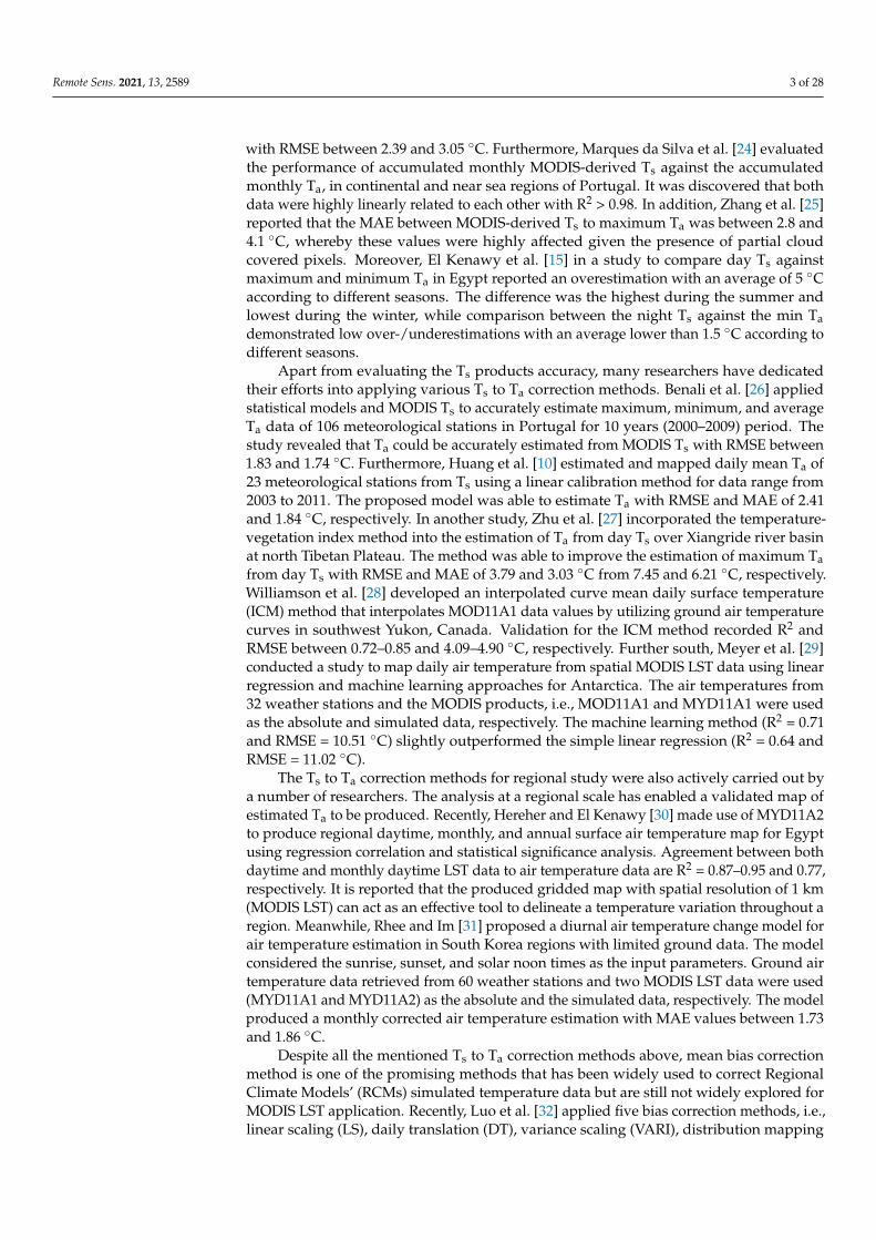
where Q1 and Q3 is the first and third quartile of the data. The extreme values exceedingthese quartiles were masked out. Then, the 8-days average Ta data were calculated byaveraging each 8-days of Ta data from 2003 until 2016. A total of 5113 daily Ta and630 8-days Ta rows data were prepared for pairing with daily Ts and 8-days Ts, respectively.Figure 2 illustrates the mean Ta distribution from 2003 to 2016. The east coast regionpossessed lower mean Ta values than the west coast region, of which the center to northernpart showed higher mean Ta than its southern counterpart.

Remote Sens. 2021, 13, 2589 7 of 28

Figure 2. Map of mean Ta distribution from 2003 to 2016.

2.3.2. Pre-Processing of Ts

The downloaded tiles were projected to WGS 1984 UTM Zone 47N and 48N. Theoriginal temperature in Kelvin (K) were then converted to degree Celsius (◦C) according toEquation (3) [38].

Ts = 0.02 T − 273.15, (3)

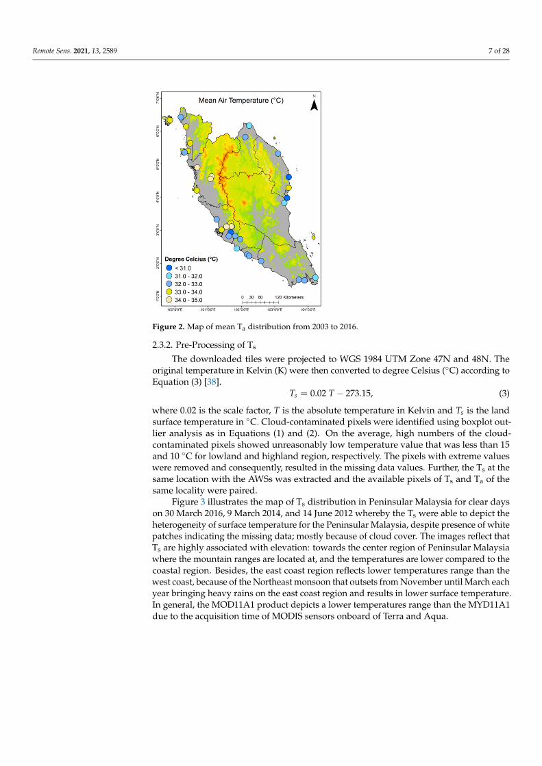
where 0.02 is the scale factor, T is the absolute temperature in Kelvin and Ts is the landsurface temperature in ◦C. Cloud-contaminated pixels were identified using boxplot out-lier analysis as in Equations (1) and (2). On the average, high numbers of the cloud-contaminated pixels showed unreasonably low temperature value that was less than 15and 10 ◦C for lowland and highland region, respectively. The pixels with extreme valueswere removed and consequently, resulted in the missing data values. Further, the Ts at thesame location with the AWSs was extracted and the available pixels of Ts and Ta of thesame locality were paired.

Figure 3 illustrates the map of Ts distribution in Peninsular Malaysia for clear dayson 30 March 2016, 9 March 2014, and 14 June 2012 whereby the Ts were able to depict theheterogeneity of surface temperature for the Peninsular Malaysia, despite presence of whitepatches indicating the missing data; mostly because of cloud cover. The images reflect thatTs are highly associated with elevation: towards the center region of Peninsular Malaysiawhere the mountain ranges are located at, and the temperatures are lower compared to thecoastal region. Besides, the east coast region reflects lower temperatures range than thewest coast, because of the Northeast monsoon that outsets from November until March eachyear bringing heavy rains on the east coast region and results in lower surface temperature.In general, the MOD11A1 product depicts a lower temperatures range than the MYD11A1due to the acquisition time of MODIS sensors onboard of Terra and Aqua.

Remote Sens. 2021, 13, 2589 8 of 28

Figure 3. The map of Ts distribution in Peninsular for selected clear days, (a) 30 March 2016, (b) 9 March 2014, and (c) 14 June2012. The Ts pixel with the same point location as the Ta AWS location was collocated together. Result in only 36 pixelswere used for each daily (MOD11A1/MYD11A1) or 8-days (MOD11A2/MYD11A2) data. The mean temperature of thecollocated pixels from MOD11A1 and MYD11A1 from 2003 to 2016 as shown in Figure 4. It can be noticed, MYD possess ahigher surface temperature range (from 30.86 to 41.65 ◦C) than MOD (from 29.13 to 38.10 ◦C). Besides, the west coastal areademonstrates a higher temperature range than the east coastal.

2.4. Region Delineation

To portray the heterogenous nature of Ta, the estimation of Ta from Ts at a regionalscale is necessary. Besides the analysis for each station, the analysis is also carried out forspecific climatic regions outlined following Suhaila and Yusop [39]. The determination ofthe boundary for each region is based from the temperature and rainfall trends and thegeographic condition of Peninsular Malaysia. The west and east regions depict differenttemperature trends as the east regions revealed lower mean temperature values than thewest region for both Ta and Ts (Figures 2–4). The Titiwangsa Range that runs through thecentral Peninsula acts as a barrier to hinder the heavy rainfall and cooler weather fromreaching the west region during the Northeast Monsoon [39]. In addition, for this study,the west region [39] is further divided into central and northcentral. This is because theKlang Valley areas (Kuala Lumpur, Putrajaya, and Central of Selangor) revealed highermean temperature values than the northcentral region (North of Selangor) [40]. Besides,the central region is associated with urban and industrial area and exhibits the effect ofurban heat island (UHI) [1,39,40]. Figure 5 illustrates the lowland areas along east and westcoast of Peninsular Malaysia (DEM = 1–60 m) that are applicable for Ts to Ta estimation

Remote Sens. 2021, 13, 2589 9 of 28

and the outline for the five regions, i.e., northwest, northcentral, central, southwest, andeast regions.

Figure 4. Mean Ts in degree Celsius (◦C) for daily MOD and MYD data from 2003 to 2016.

Figure 5. Map showing the lowland areas (0–60 m) along east and west coast regions, i.e., northwest,northcentral, central, southwest, and east regions.

Remote Sens. 2021, 13, 2589 10 of 28

Preparing Regional Data

The pre-processed Ta and Ts from 36 stations were stack as regional data according tothe information in Figure 5 and Table 2. There were 5 sets of regional datasets, and the Taand Ts were labelled as Ta_r and Ts_r, respectively.

Table 2. Region information.

Region No. of Stations Stations

Central 10 CA0058, CA0025, CA0011, CA0016, CA0054, CA0054, CA0053, CA0060, CA0010,CA0047, CA0056

East 8 CA0022, CA0059, CA0034, CA0024, CA0002, CA0015, CA0014, CA0057Northcentral 5 CA0008, CA0046, CA0041, CA0045, CA0048Northwest 8 CA0033, CA0032, CA0040, CA0017, CA0009, CA0003, CA0038, CA0020Southwest 5 CA0006, CA0043, CA0044, CA0001, CA0019

2.5. Data Analysis2.5.1. Evaluation Metrics

Four sets of Ts/Ts_r data from MOD/MYD11A1 and MOD/MYD11A2 with thesame locality as the AWSs were paired with their daily and 8-days Ta/Ts_r. Then, theevaluation was carried out in leave-two-years-out cross validation manner for both bystation and by region analysis [41]. The leave-two-years-out validation indicates that foreach station/region, 2 years data from the collocated data were excluded from the trainingset and was used as the validation set. The evaluation was repeated for 13 times withdifferent sets of leave-two-years-out data, and the results were averaged to gain the finalvalues for the evaluation metrics.

The assessment of the Ts/Ts_r against Ta/Ta_r was carried out for both pre- andpost-bias corrected data using four evaluation metrics: root mean square error (RMSE),percentage bias (PBIAS), mean absolute error (MAE), and correlation coefficient (r) [10,26].The equation for RMSE, PBIAS, MAE, and r as shown as Equations (4)–(7), respectively.

RMSE =

√√√√ 1N

N

∑i=1

(Tsi − Tai)2, (4)

where Tsi = land surface temperature data, Tai = air temperature data, and N = sample size.Root mean square error (RMSE) is a measure to determine error between two variablescomparing between simulated and observed value. A low RMSE indicates a good fitbetween two variables.

PBIAS = 100× ∑Ni=1(Tsi − Tai)

∑Ni=1 Tai

. (5)

Percentage bias (PBIAS) is a measurement of the average tendency of the simulatedvalues to be larger or smaller than the observed one. PBIAS of 0.0 indicates optimal valuewhile positive values indicate overestimation and negative values indicate underestima-tion bias.

MAE =1N

N

∑i=1|Tsi − Tai|. (6)

Mean absolute error (MAE) determines the average absolute difference between twovariables. Likewise, RMSE, a low MAE indicates a good fit between two variables.

r =∑N

i=1(Tsi − Ts

)(Tai − Ta

)√∑N

i=1(Tsi − Ts

)2∑N

i=1(Tai − Ta

)2, (7)

Remote Sens. 2021, 13, 2589 11 of 28

where Ts is the average land surface temperature data and Ta is the average air temperaturedata. Correlation coefficient, r, measures strength and direction of relationship betweenboth variables. The r value of 1 indicates a very strong positive correlation, 0 indicates nocorrelation, and −1 indicates strong negative correlation.

2.5.2. Mean Bias Correction (MBC)

There are many types of MBC method that are commonly used in climate study toreduce the error value in estimated data; they vary from the simple methods such as linearscaling, daily translation, and variance scaling to the more complicated approaches such asdistribution mapping and empirical quantile mapping [32]. In this study, linear scaling(LS-MBC) and quantile mapping (QM-MBC) techniques are used for the estimation of Tafrom Ts. Both techniques can yield high bias correction and suitable for climate study inregion with less extreme temperature range [32]. Moreover, in our study, the LS techniqueis modified by manipulating the CF values according to a number of set conditions inthe equation.

The LS-MBC technique utilizes a single correction factor retrieved from the subtractionresult between the mean observation and simulated data over a period of time [32]. Fortemperature, the simulated data are corrected by an additive function of CF. The LS-MBC can perform the correction either using monthly or daily mean value throughout theyear [34]. Nonetheless, the former is more suitable for extreme weather region with extremedaily temperature throughout the year such as in region with four seasons, while the latteris appropriate for region with moderate temperature range such as Peninsular Malaysia.Despite that, this study will examine the correction factor value from both monthly andconstant daily average. The LS-MBC are shown in Equation (8):

Tsc,d = Ts,d + (µTa − µTs), (8)

where Tsc,d is known as the corrected Ts,d for the particular d day that has undergoneadditional term from subtraction of µTa = mean Ta to µTs = mean Ts. The mean values arethe average obtained from the whole tested days and the average monthly data throughout2003 until 2016. For the correction, each AWS station will have one constant daily CFand 12 monthly CF values as in Equation (9) and the calculation can be simplified toEquation (10),

CF = (µTa − µTs) (9)

Tsc,d = Ts,d + CF. (10)

Since each station will undergo an addition of CF values as written in the LS-MBCformulation, Equation (10) will result in an over correction of bias values especially forthe Ts,d that already approximate the Ta range. Therefore, a modification of the LS-MBCformula is needed to change the bias correction method into a more robust formula.This problem could be overcome by identifying the product of Ts,d − µTa and furthermanipulation of the CF range value depending on the product of Ts,d − µTa.

The CF values are manipulated into 6 conditions, based on the positive or negativevalue of the particular CF. A larger µTa than the µTs will result in positive CF. When the CFis positive, the calculation will be as follows (Equation (11)):

Tsc,d =

Ts,d − CF, i f (Ts,d − µTa) > CF)Ts,d − 3

4 CF, i f (Ts,d − µTa >12 CF)

Ts,d − 14 CF, i f (Ts,d − µTa > 0)

Ts,d + CF, i f (Ts,d − µTa < (−CF))Ts,d +

34 CF, i f

(Ts,d − µTa <

(− 1

2 CF))

Ts,d +14 CF, Otherwise(Ts,d − µTa < 0)

. (11)

Remote Sens. 2021, 13, 2589 12 of 28

The followings are the calculation for the modified MBC, when the µTa is smaller thanthe µTs and results in negative CF values (Equation (12)):

Tsc,d =

Ts,d + CF, i f (Ts,d − µTa) > |CF|Ts,d +

34 CF, i f ( Ts,d − µTa >

∣∣∣ 12 CF

∣∣∣)Ts,d +

14 CF, i f ( Ts,d − µTa > 0)

Ts,d − CF, i f (Ts,d − µTa < CF)Ts,d − 3

4 CF, i f(

Ts,d − µTa <12 CF

)Ts,d − 1

4 CF, Otherwise (Ts,d − µTa < 0)

. (12)

Depending on the subtraction result from Ts,d − µTa as the condition, an adjustmentof CF values will take place. Each Ts,d − µTa will only satisfy one condition.

Meanwhile, quantile mapping mean bias correction (QM-MBC) works by identifyingthe empirical cumulative density functions (ecdf) of Ta as the absolute data and Ts asthe simulated data. The generated correction function depends on the quantile valuesbetween 0% and 100%. Simultaneously, the correction function is applied to unbiasednessthe Ts data according to the temperature pattern distribution [42]. The calculation can beexpressed as Equation (13) [32]:

Tsc,d = ecd f−1Ta

(ecd fTs ,d (Ts,d)), (13)

where ecd f−1 denotes the inverse ecd f .

3. Results3.1. Evaluation Metrics for Pre- and Post-MBC against Ta by Station3.1.1. RMSE

Table 3 tabulates the maximum, minimum, and average value of RMSE, MAE, PBIAS,and r for pre-MBC (Ts), post-MBC linear scaling using constant daily CF (Tscd), post-MBClinear scaling using monthly CF (Tscm) and post-MBC quantile mapping (Tscq) against Taaccording to the leave-two-years-out evaluation for 36 AWS station. For the pre-MBC (Ts),the average RMSE values were much higher for the MYD products (MYD11A1/11A2), i.e.,5.13 and 5.09 ◦C compared to the MOD products (MOD11A1/MOD11A2), i.e., 3.42 and3.48 ◦C. The error value for MYD products was approximately 1.5 times higher than theMOD products. Generally, the same pattern was observed for the maximum and minimumRMSE values.

On the contrary, the average RMSE values of all post-MBC products (Tscd, Tscm, andTscq) depicted lower error range compared to the pre-MBC products (Ts), ranging from2.11 to 2.39 ◦C, 2.06 to 2.35 ◦C, and 2.07 to 2.74 ◦C for Tscd, Tscm, and Tscq, respectively.For all post-MBC products, the 8-days MOD/MYD11A2 showed lower average RMSEvalues (Tscd = 2.11 ◦C/2.32 ◦C, Tscm = 2.06 ◦C/2.31 ◦C, and Tscq = 2.12 ◦C/2.07 ◦C) thanthe daily MOD/MYD11A1 (Tscd = 2.39 ◦C/2.37 ◦C, Tscm = 2.35 ◦C/2.34 ◦C, and Tscq= 2.74 ◦C/2.67 ◦C). Moreover, the same pattern was shown for the maximum RMSEvalues. The maximum RMSE values for the 8-days MOD/MYD11A2 were recordedlower, i.e., 3.04 ◦C/3.07 ◦C, 3.00 ◦C/3.20 ◦C, and 3.66 ◦C/3.57 ◦C compared to the dailyMOD/MYD11A2, i.e., 3.56 ◦C/3.86 ◦C, 3.54 ◦C/3.71 ◦C, and 4.37 ◦C/4.34 ◦C for Tscd, Tscm,and Tscq, respectively.

A greater detail as illustrated in Figure 6 revealed that for pre-MBC (Ts), MOD11A1/11A2had lower RMSE values ranging from 1.85 to 5.83 ◦C with only three of the stations showingRMSE > 5 ◦C: CA0002 for MOD11A1 and CA0019 and CA0058 for MOD11A2. Meanwhile,MYD11A1/11A2 depicted higher RMSE values ranging from 2.37 to 8.28 ◦C with 54.67% ofthe stations showing RMSE > 5 ◦C. MYD11A1/MYD11A2 data exhibited 21 and 18 stationswith RMSE > 5 ◦C. Generally, the distribution of stations with higher RMSE values wasmainly in the west coast region rather than the east coast region.

Remote Sens. 2021, 13, 2589 13 of 28

Table 3. RMSE, MAE, PBIAS, and r for pre-MBC (Ts), post-MBC linear scaling using constant daily CF (Tscd), post-MBClinear scaling using monthly CF (Tscm), and post-MBC quantile mapping (Tscq) against Ta according to the leave-two-years-out evaluation for 36 AWS station.

Pre-MBCTs

Post-MBC LS(Daily CF) Tscd

Post-MBC LS(Monthly CF) Tscm

Post-MBCQM Tscq

Metrics Av. Max Min Av. Max Min Av. Max Min Av. Max Min

RMSE(◦C)

MOD11A13.42 5.83 1.85 2.39 3.56 1.48 2.35 3.54 1.48 2.74 4.37 1.87

MOD11A23.48 5.12 2.15 2.11 3.04 1.57 2.06 3.00 1.45 2.12 3.66 1.28

MYD11A1 5.13 7.34 2.37 2.37 3.86 1.43 2.34 3.71 1.43 2.67 4.34 1.77

MYD11A2 5.09 8.28 2.47 2.32 3.07 1.65 2.31 3.20 1.69 2.07 3.57 1.24

PBIAS(%)

MOD11A11.36 9.90 −14.27 −1.85 2.43 −6.33 −1.47 2.10 −5.63 −3.20 −0.62 −6.11

MOD11A24.40 14.22 −11.70 0.97 3.76 −3.55 1.20 3.82 −2.85 −0.37 1.20 −2.11

MYD11A1 8.88 22.02 −11.77 −0.17 3.35 −6.34 0.21 3.15 −5.51 −3.26 −1.07 −5.51

MYD11A210.74 25.56 −6.74 2.46 4.78 −3.37 2.55 4.73 −2.71 −0.42 1.02 −1.65

MAE(◦C)

MOD11A12.88 5.20 1.46 1.94 3.15 1.19 1.90 3.17 1.21 2.23 3.71 1.46

MOD11A23.01 4.65 1.71 1.73 2.54 1.23 1.68 2.62 1.12 1.74 3.11 1.00

MYD11A1 4.56 7.09 1.86 1.92 3.10 1.23 1.90 3.07 1.18 2.16 3.64 1.38

MYD11A2 4.57 7.97 1.97 1.90 2.62 1.41 1.87 2.66 1.39 1.69 3.07 0.97

r

MOD11A10.24 0.47 0.04 0.23 0.48 0.01 0.30 0.54 0.08 0.24 0.48 0.04

MOD11A20.20 0.43 0.01 0.18 0.42 0.00 0.29 0.52 −0.04 0.20 0.44 0.01

MYD11A1 0.28 0.48 0.08 0.27 0.49 0.06 0.31 0.62 −0.02 0.29 0.49 0.08

MYD11A2 0.20 0.42 −0.04 0.20 0.42 −0.08 0.27 0.56 −0.06 0.21 0.43 −0.05

Nonetheless, the RMSE distributions for post-MBC products (Tscd, Tscm, and Tscq)showed that the majority of the RMSE values were between 1 and 3 ◦C. Specifically, forTscd and Tscm, only 9.72%/12.50% and 6.94%/9.72 stations showed RMSE value > 3 ◦C forMOD11A1/11A2 and MYD11A1/11A2, respectively. Meanwhile, for Tscq, 16.67% stationsshowed RMSE values > 3 ◦C for both MOD11A1/2 and MYD11A1/2. Lower numbers ofstations with RMSE values > 3 ◦C were recorded for the 8-days MOD/MYD11A2 (Tscd = 1and 3 stations, Tscm = 1 and 2 stations, and Tscq = 3 stations for both) than the dailyMOD/MYD11A1 (Tscd = 6 stations for both, Tscm = 4 and 5 stations, and Tscq = 9 stationsfor both).

3.1.2. PBIAS

Assessing the average PBIAS values in Table 3, the pre-MBC Ts products tended tooverestimate the Ta. The average PBIAS of MOD11A1 and MOD11A2 depicted lowervalues (1.36% and 4.40%) than the MYD11A1 and MYD11A2 (8.88% and 10.74%). Thesame trend was observed for the maximum PBIAS values as MYD11A1 and MYD11A2manifested high maximum PBIAS of 22.02% and 25.56%, respectively, while MOD11A1 andMOD11A2 showed low maximum PBIAS of 9.90% and 14.22%, respectively. In contrast, forthe minimum PBIAS values, MOD11A1 and MOD11A2 recorded −14.27% and −11.70%,suggesting higher magnitudes of underestimation in comparison to the MYD11A1 andMYD11A2 that had −11.77% and −6.74%. It can be noted that MOD11A1 demonstratedthe highest minimum and lowest maximum and average PBIAS, while MYD11A2 depictedthe lowest minimum and highest maximum and average PBIAS.

Remote Sens. 2021, 13, 2589 14 of 28

Figure 6. Distribution of RMSE for comparison between simulated data, (a) Ts, (b) Tscd, (c) Tscm, and (d) Tscq, and observeddata, Ta.

Meanwhile, the average PBIAS values for the post-MBC (Tscd, Tscm, and Tscq) exhib-ited reduced over-/underestimations with average PBIAS values between −1.85% and2.46%, −1.47% and 2.55%, and −3.26% and −0.37%, respectively. In particular, the dailyMOD11A1 depicted negative average PBIAS values (Tscd = −1.85%, Tscm = −1.47%, and

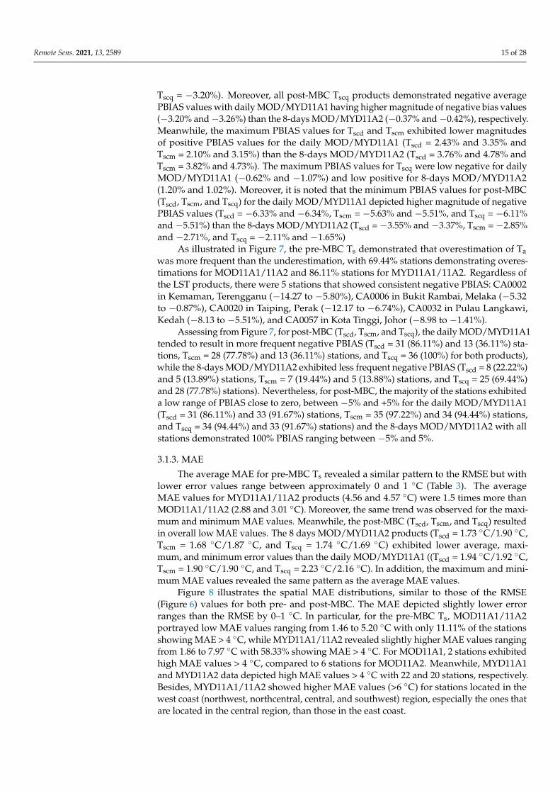
Remote Sens. 2021, 13, 2589 15 of 28

Tscq = −3.20%). Moreover, all post-MBC Tscq products demonstrated negative averagePBIAS values with daily MOD/MYD11A1 having higher magnitude of negative bias values(−3.20% and−3.26%) than the 8-days MOD/MYD11A2 (−0.37% and−0.42%), respectively.Meanwhile, the maximum PBIAS values for Tscd and Tscm exhibited lower magnitudesof positive PBIAS values for the daily MOD/MYD11A1 (Tscd = 2.43% and 3.35% andTscm = 2.10% and 3.15%) than the 8-days MOD/MYD11A2 (Tscd = 3.76% and 4.78% andTscm = 3.82% and 4.73%). The maximum PBIAS values for Tscq were low negative for dailyMOD/MYD11A1 (−0.62% and −1.07%) and low positive for 8-days MOD/MYD11A2(1.20% and 1.02%). Moreover, it is noted that the minimum PBIAS values for post-MBC(Tscd, Tscm, and Tscq) for the daily MOD/MYD11A1 depicted higher magnitude of negativePBIAS values (Tscd = −6.33% and −6.34%, Tscm = −5.63% and −5.51%, and Tscq = −6.11%and−5.51%) than the 8-days MOD/MYD11A2 (Tscd =−3.55% and−3.37%, Tscm =−2.85%and −2.71%, and Tscq = −2.11% and −1.65%)

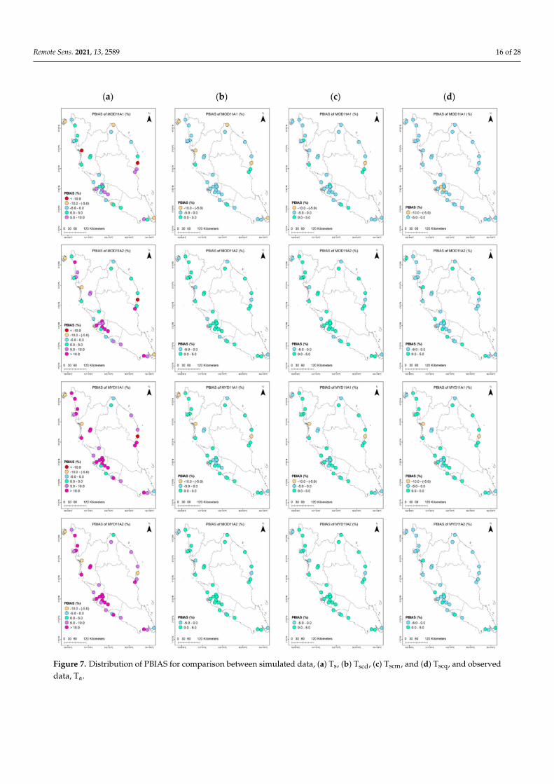
As illustrated in Figure 7, the pre-MBC Ts demonstrated that overestimation of Tawas more frequent than the underestimation, with 69.44% stations demonstrating overes-timations for MOD11A1/11A2 and 86.11% stations for MYD11A1/11A2. Regardless ofthe LST products, there were 5 stations that showed consistent negative PBIAS: CA0002in Kemaman, Terengganu (−14.27 to −5.80%), CA0006 in Bukit Rambai, Melaka (−5.32to −0.87%), CA0020 in Taiping, Perak (−12.17 to −6.74%), CA0032 in Pulau Langkawi,Kedah (−8.13 to −5.51%), and CA0057 in Kota Tinggi, Johor (−8.98 to −1.41%).

Assessing from Figure 7, for post-MBC (Tscd, Tscm, and Tscq), the daily MOD/MYD11A1tended to result in more frequent negative PBIAS (Tscd = 31 (86.11%) and 13 (36.11%) sta-tions, Tscm = 28 (77.78%) and 13 (36.11%) stations, and Tscq = 36 (100%) for both products),while the 8-days MOD/MYD11A2 exhibited less frequent negative PBIAS (Tscd = 8 (22.22%)and 5 (13.89%) stations, Tscm = 7 (19.44%) and 5 (13.88%) stations, and Tscq = 25 (69.44%)and 28 (77.78%) stations). Nevertheless, for post-MBC, the majority of the stations exhibiteda low range of PBIAS close to zero, between −5% and +5% for the daily MOD/MYD11A1(Tscd = 31 (86.11%) and 33 (91.67%) stations, Tscm = 35 (97.22%) and 34 (94.44%) stations,and Tscq = 34 (94.44%) and 33 (91.67%) stations) and the 8-days MOD/MYD11A2 with allstations demonstrated 100% PBIAS ranging between −5% and 5%.

3.1.3. MAE

The average MAE for pre-MBC Ts revealed a similar pattern to the RMSE but withlower error values range between approximately 0 and 1 ◦C (Table 3). The averageMAE values for MYD11A1/11A2 products (4.56 and 4.57 ◦C) were 1.5 times more thanMOD11A1/11A2 (2.88 and 3.01 ◦C). Moreover, the same trend was observed for the maxi-mum and minimum MAE values. Meanwhile, the post-MBC (Tscd, Tscm, and Tscq) resultedin overall low MAE values. The 8 days MOD/MYD11A2 products (Tscd = 1.73 ◦C/1.90 ◦C,Tscm = 1.68 ◦C/1.87 ◦C, and Tscq = 1.74 ◦C/1.69 ◦C) exhibited lower average, maxi-mum, and minimum error values than the daily MOD/MYD11A1 ((Tscd = 1.94 ◦C/1.92 ◦C,Tscm = 1.90 ◦C/1.90 ◦C, and Tscq = 2.23 ◦C/2.16 ◦C). In addition, the maximum and mini-mum MAE values revealed the same pattern as the average MAE values.

Figure 8 illustrates the spatial MAE distributions, similar to those of the RMSE(Figure 6) values for both pre- and post-MBC. The MAE depicted slightly lower errorranges than the RMSE by 0–1 ◦C. In particular, for the pre-MBC Ts, MOD11A1/11A2portrayed low MAE values ranging from 1.46 to 5.20 ◦C with only 11.11% of the stationsshowing MAE > 4 ◦C, while MYD11A1/11A2 revealed slightly higher MAE values rangingfrom 1.86 to 7.97 ◦C with 58.33% showing MAE > 4 ◦C. For MOD11A1, 2 stations exhibitedhigh MAE values > 4 ◦C, compared to 6 stations for MOD11A2. Meanwhile, MYD11A1and MYD11A2 data depicted high MAE values > 4 ◦C with 22 and 20 stations, respectively.Besides, MYD11A1/11A2 showed higher MAE values (>6 ◦C) for stations located in thewest coast (northwest, northcentral, central, and southwest) region, especially the ones thatare located in the central region, than those in the east coast.

Remote Sens. 2021, 13, 2589 16 of 28

Figure 7. Distribution of PBIAS for comparison between simulated data, (a) Ts, (b) Tscd, (c) Tscm, and (d) Tscq, and observeddata, Ta.

Remote Sens. 2021, 13, 2589 17 of 28

Figure 8. Distribution of MAE for comparison between simulated data, (a) Ts, (b) Tscd, (c) Tscm, and (d) Tscq, and observeddata, Ta.

In contrast, the MAE distribution for post-MBC (Tscd, Tscm, and Tscq), as illustrated inFigure 8, revealed consistent low MAE values for all products, i.e., Tscd = 1.19 to 3.15 ◦C,Tscm = 1.12 to 3.17 ◦C, and Tscq = 0.97 to 3.71 ◦C. The majority of the stations for all post-

Remote Sens. 2021, 13, 2589 18 of 28

MBC products showed MAE < 3 ◦C with only a number of stations recording > 3 ◦C(Tscd = 3 stations, Tscm = 2 stations, and Tscq = 10 stations).

3.1.4. Correlation Coefficient (r)

Table 3 tabulates very low average r values for all pre-MBC Ts products, of whichthe daily MOD/MYD11A1 depicted a slightly higher average r value than the 8-daysMOD/MYD11A2 with 0.24–0.28 and 0.20, respectively. A similar pattern was observed forthe maximum r values whereby the daily MOD/MYD11A1 and 8-days MOD/MYD11A2showed a maximum r of 0.47 and 0.48 for MOD11A1 and MYD11A1, while a maximumr value for MOD11A2 and MYD11A2 was 0.43 and 0.42, respectively. Moreover, theminimum r values were observed to be very close to zero for both 8-days MOD and MYD(0.01 and −0.04) and daily MOD and MYD (0.04 and 0.08). Moreover, the r values for thepost-MBC products (Tscd, Tscm, and Tscq) revealed the same scenarios, as the average rvalues for daily MOD/MYD11A1 (Tscd = 0.23/0.27, Tscm = 0.30/0.31, and Tscq = 0.24/0.29)were slightly higher than the 8-days MOD/MYD11A2(Tscd =0.18/0.20, Tscm = 0.29/0.27,and Tscq = 0.20/0.21). The maximum r values demonstrated a moderate r range from0.42 to 0.49, 0.52 to 0.62, and 0.43 to 0.48 for Tscd, Tscm, and Tscq, respectively, while theminimum r values demonstrated very near to zero r values ranging from −0.08 to 0.06,−0.06 to 0.08, and −0.05 to 0.08 for Tscd, Tscm, and Tscq, respectively.

For pre-MBC Ts products, moderate r values (>0.3) were more frequent in the dailyMOD and MYD than the 8-days MOD and MYD products (Figure 9). The moderate rvalues (>0.3) were recorded at 10 and 14 stations for each daily MOD and MYD and at 6 and10 stations for 8-days MOD and MYD, respectively. Meanwhile, for post-MBC products,Tscm resulted in highest total numbers of stations (MOD/MYD11A1 and MOD/MYD11A2)with moderate r values >0.3, followed by Tscq and Tscd with 66, 39, and 32 stations, re-spectively. Furthermore, the stations with moderate r values (>0.5) were only observed inthe Tscm products (MOD11A1/11A2 = 7 stations and MYD11A1/11A2 = 5 stations) with rvalue ranging between 0.51 and 0.62.

3.2. Evaluation Metrics for Pre- and Post-MBC against Ta by Region3.2.1. RMSE

Table 4 tabulates the maximum, minimum, and average value of RMSE, MAE, PBIAS,and r from pre-MBC (Ts_r), post-MBC linear scaling using constant daily CF (Tscd_r),post-MBC linear scaling using monthly CF (Tscm_r), and post-MBC quantile mapping(Tscq_r) against Ta_r according to the leave-two-years-out evaluation for 5 regions. Thetabulated data indicated that the average RMSE values for the pre-MBC Ts_r of the by regioncomparison reflect same pattern as the by station comparison. The MYD products (5.23 and5.42 ◦C) indicate 1.5 times higher error than the MOD (3.33 and 3.55 ◦C). The same patternis shown by maximum and minimum RMSE values. Meanwhile, the post-MBC productsshowed an overall low average RMSE < 3 ◦C. Specifically, the RMSE range values wererecorded between 1.96 and 3.71 ◦C, 1.95 and 3.51 ◦C, and 1.88 and 3.61 ◦C for Tscd_r, Tscm_r,and Tscq_r, respectively. Figure 10 illustrates the RMSE for pre- and post-MBC products. Itcan be observed that the error values were well reduced for all regions and products.

Remote Sens. 2021, 13, 2589 19 of 28

Figure 9. Distribution of r for comparison between simulated data, (a) Ts, (b) Tscd, (c) Tscm, and (d) Tscq, and observeddata, Ta.

Remote Sens. 2021, 13, 2589 20 of 28

Table 4. RMSE, MAE, PBIAS, and r from by region comparison for pre-MBC (Ts_r), post-MBC linear scaling using constantdaily CF (Tscd_r), post-MBC linear scaling using monthly CF (Tscm_r), and post-MBC quantile mapping (Tscq_r) against Ta_r

according to the leave-two-years-out evaluation.

Pre-MBCTs_r

Post-MBC LS(Daily CF) Tscd_r

Post-MBC LS(Monthly CF) Tscm_r

Post-MBCQM Tscq_r

Metrics Av. Max Min Av. Max Min Av. Max Min Av. Max Min

RMSE(◦C)

MOD11A13.33 3.87 2.90 2.70 3.71 1.96 2.71 3.51 1.95 2.55 3.05 2.19

MOD11A23.55 3.74 2.85 2.54 3.14 2.01 2.52 3.03 2.00 2.26 2.76 1.88

MYD11A1 5.23 5.63 4.94 2.60 3.37 2.07 2.64 3.44 2.10 2.66 3.61 2.05

MYD11A2 5.42 6.14 5.20 2.70 3.18 2.31 2.69 3.21 2.32 2.26 2.79 1.92

PBIAS(%)

MOD11A12.42 5.22 0.29 −0.75 0.39 −1.91 −0.62 0.30 −1.93 −2.31 −1.81 −2.73

MOD11A25.75 9.06 3.40 2.06 3.48 −0.22 2.09 3.31 −0.16 −0.04 0.37 −0.91

MYD11A110.19 14.21 7.63 1.61 2.33 0.78 1.78 2.75 1.20 −1.89 −0.61 −3.18

MYD11A212.07 16.53 9.20 4.30 5.27 3.18 4.26 5.15 3.22 0.37 1.16 −0.74

MAE(◦C)

MOD11A12.79 3.27 2.36 2.21 3.10 1.60 2.21 2.90 1.61 1.99 2.46 1.74

MOD11A23.09 3.36 2.37 2.12 2.64 1.66 2.10 2.58 1.67 1.79 2.13 1.50

MYD11A1 4.68 5.22 4.36 2.15 2.79 1.71 2.18 2.84 1.73 2.08 2.76 1.63

MYD11A2 4.89 5.75 4.60 2.27 2.73 1.92 2.27 2.76 1.93 1.78 2.16 1.51

r

MOD11A10.23 0.25 0.19 0.23 0.26 0.19 0.25 0.27 0.21 0.29 0.45 0.17

MOD11A20.16 0.24 0.11 0.19 0.31 0.11 0.24 0.33 0.17 0.26 0.40 0.13

MYD11A1 0.29 0.32 0.27 0.26 0.31 0.19 0.29 0.33 0.25 0.29 0.52 0.06

MYD11A2 0.17 0.26 0.12 0.19 0.25 0.14 0.25 0.39 0.15 0.25 0.46 0.12

Figure 10. Comparison of evaluation metrics score between Ts_r, Tscd_r, Tscm_r, and Tscq_r against Ta_r.

Remote Sens. 2021, 13, 2589 21 of 28

3.2.2. PBIAS

The average PBIAS values for pre-MBC Ts_r was lower for MOD products than thosefor the MYD products by 2.42%/5.75% and 10.19%/12.07%, respectively (Table 4). Thesame was observed for maximum and minimum values. The maximum values wererecorded at 5.22%/9.06% and 14.21%/16.53% for MOD11A1/11A2 and MYD11A1/11A2products, respectively, while the minimum values were at 0.29%/3.40% and 7.63%/9.20%for MOD11A1/11A2 and MYD11A1/11A2 products, respectively. The post-MBC products(Tscd_r, Tscm_r, and Tscq_r) tabulated an overall average PBIAS values < 5% with averagePBIAS range between −0.75% and 4.30%, −0.62% and 4.26%, and −2.31% and 0.37% forTscd_r, Tscm_r, and Tscm_r, respectively. Spatially, post-MBC product of MOD11A1 illustratednegative PBIAS values for almost all region (Tscd_r =−1.91% to 0.39%, Tscm_r = −1.93% to 0.30%,and Tscq_r = −2.73% to −1.81%) (Figure 10). Besides, for MYD11A1, the Tscq_r tended toresult in negative PBIAS values for all regions with range between −3.18% and −0.61%.Overall, the post-MBC products showed a well reduced bias for MOD11A2, MYD11A1,and MYD11A2.

3.2.3. MAE

A similar pattern was observed between pre-MBC Ts_r MAE and RMSE values asthe MYD products result in 1.5 times higher error values than the MOD (Table 4). Theaverage values were recorded at 2.79/3.09 ◦C and 4.68/4.89 ◦C for MOD11A1/11A2and MYD11A1/11A2 products, respectively. The maximum and minimum MAE valuesrevealed two different range of error values between the MOD and MYD products, i.e., 2.36to 5.75 ◦C and 4.36 to 5.75 ◦C, respectively. The post-MBC products depicted an overalllow average MAE value < 2.5 ◦C (Tscd_r = 2.12 to 2.27 ◦C, Tscm_r = 2.10 to 2.27 ◦C, andTscq_r = 1.78 to 2.08 ◦C). Figure 10 showed an apparent reduction in MAE values betweenthe pre- and post-MBC products except for MOD11A1.

3.2.4. Correlation Coefficient (r)

The r values observed from Table 4 illustrated low r values for all pre-MBC productswith average r between 0.16 and 0.29. In detail, the daily products tabulated slightly higherr range between 0.23 and 0.29 than the 8-days products with r range between 0.16 and 0.17.The post-MBC products showed a slight improvement in the r values with Tscq_r revealingthe highest r range for average and maximum values (average = 0.25 to 0.29 and maximum= 0.40 to 0.52), followed by Tscm_r (average = 0.24 to 0.29 and maximum = 0.27 to 0.39) andTscd_r (average = 0.19 to 0.26 and maximum = 0.25 to 0.31).

Figure 10 shows that the performance of post-MBC varies according to the region.Notably, the Tscq_r performed best for central and northcentral region. Other than that, anoverall slightly improved r values can be observed throughout the MBC products.

4. Discussion4.1. By Station Performance

The assessment of MODIS Ts against Ta (pre-MBC) indicated high variabilities in therelationship between both data. For instance, MOD11A1 was found to have the closestrelationship to Ta data with the lowest average RMSE of 3.42 ◦C and PBIAS of 1.36%,followed by MOD11A2 with RMSE of 3.48 ◦C and PBIAS of 4.40%, MYD11A1 with RMSEof 5.13 ◦C and PBIAS of 8.88% and finally, MYD11A2 with average RMSE of 5.09 ◦C andhighest PBIAS of 10.74%. These metrics suggested that MOD11A1/11A2 was better atestimating the Ta than MYD11A1/11A2. This could be attributed to the time of dataacquisition. The former is acquired at 10:30 a.m. local time, while the latter is acquired at1:30 p.m. local time whereby later in the noon, solar activity for the tropical region suchas Peninsular Malaysia is the highest. Consequently, the MOD data are a better proxy formaximum daily Ta given that the MYD Ts tended to overestimate the Ta.

Additionally, the daily Ts, i.e., MOD/MYD11A1 and 8-days Ts, i.e., MOD/MYD11A2depicted different characteristics of performance as the former illustrated lower errors and

Remote Sens. 2021, 13, 2589 22 of 28

lower under-/overestimations than the latter. Daily data are known to be better at esti-mating Ta than 8-days data due to the inconsistency of the numbers of days used to countthe 8-days Ts [38]. Although the 8-days Ta are averaged from the daily Ta for a completeduration of 8-days, 8-days Ts are subject to missing data resulted from cloud coverage andhence, could be averaged from daily data as low as from 2 to 8 days. This inconsistency isbelieved to contribute to low accuracies in estimation between both datasets.

Furthermore, although researchers such as El Kenawy et al. [15] recommended thatcorrections of Ts against Ta were needed if only the score of PBIAS > ± 5%, the usageof MOD11A1 (average PBIAS = 1.36%) for lowland area in Peninsular Malaysia regionwithout any correction to represent the Ta can still be considered inappropriate given itsaverage error (3.42 ◦C) is too large to be considered for many applications [43].

Post-MBC (Tscd, Tscm, and Tscq) data assessment against Ta depicted better estimationswith three of the evaluation metric’s parameters showing significant improvements in theerror and bias values, while the correlation coefficient (r) showing a moderate improvementin the r values. All post-MBC products demonstrated average low RMSEs range (Tscd = 2.11to 2.39 ◦C, Tscm = 2.06 to 2.35 ◦C, and Tscq = 2.07 to 2.74 ◦C), average low PBIAS range(Tscd = −1.85 to 2.46%, Tscm = −1.47 to 2.55%, and Tscq = −3.26 to −0.37%), and lowaverage MAE range (Tscd = 1.73 to 1.94 ◦C, Tscm = 1.68 to 1.90 ◦C, and Tscq = 1.69 to 2.23 ◦C).Meanwhile, the r scores demonstrated a slight improvement in the r values from theaverage range for pre-MBC (0.20–0.28) to average range for post-MBC (Tscm = 0.27–0.31 andTscq = 0.20–0.29), except for Tscd with r average range between 0.18 and 0.27. According toYan et al. [43], estimated products at RMSE approximately < 3 ◦C are considered acceptable,and most of the recent studies for Ta estimation reported RMSE values < 3 ◦C.

Although the modified MBC demonstrated a good performance at reducing PBIASover-/underestimation range, the underestimation in the MOD11A1 data was significantlyhigh in post-MBC, i.e., Tscd = 86.11%, Tscm = 77.78%, and Tscq = 100% versus pre-MBC,i.e., 61.11%. A possible explanation for this is because for pre-MBC, the MOD11A1 Tsand Ta temperature range were already close to each other and hence, the applicationof the MBC tended to overcorrect the MOD11A1 Ts and result in higher magnitude ofunderestimation. Contrarily, the MBC only contributed a slight change for the post-MBC rvalues. This is because the application of the MBC technique could only adjust the rangeof the Ts values by shifting the Ts values towards the Ta according to the CF values thatsatisfy the condition given (for LS-MBC) or according to the respective quantile calculation(for QM-MBC) without changing the original temporal pattern of the Ts data. While thesetechniques have resulted in a significant improvement of error and bias terms for the Tscd,Tscm, and Tscq against Ta, the relationship between both datasets showed a moderate tono improvement.

Additionally, the assessment on post-MBC (Tscd, Tscm, and Tscq) showed that rangesfor error and bias values were not as high as in the pre-MBC data. All post-MBC Tscd,Tscm, and Tscq products depicted low and similar ranges of average bias and errors (av-erage RMSE and MAE < 3 ◦C and average PBIAS between −5% and 5%), while thepre-MBC demonstrated that the MYD11A1/11A2 Ts had higher error (average RMSE andMAE = 4.56 to 5.13 ◦C) and bias (PBIAS = 8.88 to 10.74%) range than the MOD11A1/11A2(average RMSE and MAE = 2.88 to 3.48 ◦C, PBIAS = 1.36 to 4.40%). This suggested thatboth MBC approaches (LS-MBC and QM-MBC) were suitable for all types of MODIS Tstested in this study.

For comparison, Figure 11 displays the boxplot presentation for the average tempera-ture values between pre (Ts) and post-MBC (Tscd, Tscm, and Tscq) against Ta from 36 AWS.Significant improvements could be observed in the post-MBC values as the range of Tshas decreased tremendously approaching the range of Ta with Tscq depicting the mostapproximate temperature range to the Ta. This indicates that the QM-MBC method cancapture well the distribution of Ta by removing the biases by quantile [44] rather than theLS-MBC technique that removes the biases using CF values from overall constant dailyand monthly values.

Remote Sens. 2021, 13, 2589 23 of 28

Figure 11. Comparison of average temperature value between Ta, Ts, Tscd, Tscm, and Tscq forMOD11A1, MOD11A2, MYD11A1, and MYD11A2 across 36 AWS.

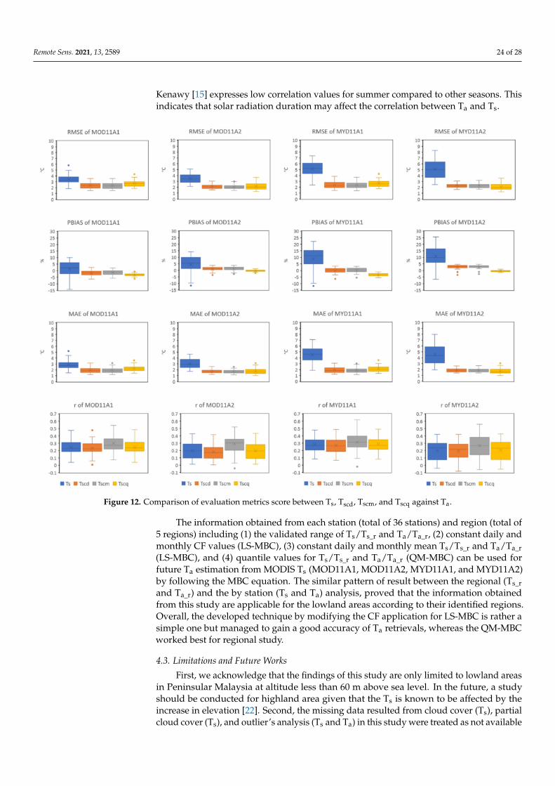
Figure 12 illustrates the boxplot presentation of evaluations metrics score betweenTs, Tscd, Tscm, and Tscq against Ta for 36 AWSs. The bias correction method consistentlyreduced the RMSE and MAE to 2–5 ◦C and 1–4 ◦C, respectively. The PBIAS also showed areasonable reduction in the over-/underestimation to range of bias between −6.34% and4.78%. In comparison, Tscd, Tscm, and Tscq demonstrated a small- range of error and bias,but not for r. Tscm showed highest improvement in r values than the Tscd and Tscq. Thisindicates that although these post-MBC products produced an acceptable result for Taapproximation, the application of LS-MBC technique using the monthly CF was betterthan the constant daily CF (Tscd) and quantile mapping technique (Tscq). This is becauseapplication of monthly CF is calculated from a more detail calculation (by month) than thedaily CF that is calculated using single CF for the whole 13 years. Application of monthlyCF enable changes in temperature according to the changes in the monsoon season, ifpresent, to be applied.

4.2. By Region Performance

Figure 13 displays the comparison between evaluation metrics between Ts_r, Tscd_r,Tscm_r, and Tscq_r against Ta_r for 5 regions. The LS and QM-MBC has tremendouslyreduced the bias and error values as the boxplot for post-MBC (Tscd_r, Tscm_r, and Tscq_r)were located nearer to zero value than the pre-MBC (Ts_r). Meanwhile, the r valuesdepicted modest improvement with the r maximum values pre-MBC (Ts_r = 0.24–0.32)slightly increased (Tscd_r = 0.25–0.31, Tscm_r = 0.27–0.39, and Tscq_r = 0.40–0.52).

Moreover, the Tscq_r depicted the most improved values of RMSE, MAE, and PBIAS.This indicates that QM-MBC can perform better when more data are stack together (regionaldata). With more collocated pixels, the temperature distribution can be better defined,resulting in better quantile calculation [32,33]. The same pattern was observed for r asTscq_r showed the highest improvement of r for MOD11A1, MOD11A2, and MYD11A2.

The low correlation coefficient (r) for both pre- and post-MBC data compared to Ta,despite the low RMSE obtained for post-MBC are possible and acceptable. In this study,the reason for low r values could be because of the low temperature range for between10 and 15 ◦C and less variation in the temperature pattern [16]. In the tropic region, thereare only two distinct seasons, the hot and dry and cold and wet season driven by thetwo monsoonal wind seasons, i.e., the Southwest and Northeast monsoons. Besides, El

Remote Sens. 2021, 13, 2589 24 of 28

Kenawy [15] expresses low correlation values for summer compared to other seasons. Thisindicates that solar radiation duration may affect the correlation between Ta and Ts.

Figure 12. Comparison of evaluation metrics score between Ts, Tscd, Tscm, and Tscq against Ta.

The information obtained from each station (total of 36 stations) and region (total of5 regions) including (1) the validated range of Ts/Ts_r and Ta/Ta_r, (2) constant daily andmonthly CF values (LS-MBC), (3) constant daily and monthly mean Ts/Ts_r and Ta/Ta_r(LS-MBC), and (4) quantile values for Ts/Ts_r and Ta/Ta_r (QM-MBC) can be used forfuture Ta estimation from MODIS Ts (MOD11A1, MOD11A2, MYD11A1, and MYD11A2)by following the MBC equation. The similar pattern of result between the regional (Ts_rand Ta_r) and the by station (Ts and Ta) analysis, proved that the information obtainedfrom this study are applicable for the lowland areas according to their identified regions.Overall, the developed technique by modifying the CF application for LS-MBC is rather asimple one but managed to gain a good accuracy of Ta retrievals, whereas the QM-MBCworked best for regional study.

4.3. Limitations and Future Works

First, we acknowledge that the findings of this study are only limited to lowland areasin Peninsular Malaysia at altitude less than 60 m above sea level. In the future, a studyshould be conducted for highland area given that the Ts is known to be affected by theincrease in elevation [22]. Second, the missing data resulted from cloud cover (Ts), partialcloud cover (Ts), and outlier’s analysis (Ts and Ta) in this study were treated as not available

Remote Sens. 2021, 13, 2589 25 of 28

(NA). To overcome the gaps in Ts data, interpolation [45], similar pixel method [46], datafusion [47], or machine learning [48] have been applied in other works but not in our studythat only used original datasets. Finally, we acknowledge the limitation in delivering thecorrection factor values given unknown gaps in the constant daily and monthly Ts, asopposed to Yoo et al. [49] who performed linear interpolation. Addressing further, thesecond and third gaps can possibly avoid distorted CF values and thus give better results.

Figure 13. Comparison of evaluation metrics score between Ts_r, Tscd_r, Tscm_r, and Tscq_r against Ta_r.

5. Conclusions

This study found that (1) the error values for pre-MBC Ts in comparison to the Ta werehigh especially for the MYD11A1/11A2 than the MOD11A1/11A2; chiefly due to differentacquisition times that is influenced by solar activity. (2) The high bias and error valuesfor the pre-MBC Ts suggested that the application of correction is necessary. (3) The MBCfor station analysis (Tscd, Tscm, and Tscq) has successfully reduced the errors and biases inpre-MBC (Ts), i.e., average RMSE values from 3.42–5.13 to 2.06–2.74 ◦C, average PBIASvalues from 1.36–10.74% to −3.26–2.55%, and average MAE values from 2.88–4.57 ◦C to1.68–2.23 ◦C. While, the average r values depicted slight improvement from 0.20–0.28 to0.18–0.31. (4) The pattern is the same for by region analysis (Tscd_r, Tscm_r, and Tscq_r),i.e., average RMSE values from 3.33–5.42 to 2.26–2.71 ◦C, average PBIAS values from2.42–12.07% to −2.31–4.30%, average MAE values from 2.79–4.89 to 1.78–2.27 ◦C, andaverage r value from 0.16–0.29 to 0.19–0.29. (5). Both MBC methods (LS-MBC and QMMBC) resulted in an acceptable range of correction but by a comparison, the MBC using

Remote Sens. 2021, 13, 2589 26 of 28

monthly CF depicted a slightly better correction than the MBC using daily constant CF,while QM-MBC worked best for regional study. This study also illustrated that althoughthe proposed LS-MBC technique in this study is rather a simple mathematical equation thanthe more sophisticated QM-MBC technique, it was adequate for improving the estimationTa from MODIS Ts for a tropical region.

Author Contributions: Conceptualization, F.M.M. and N.M.; methodology, N.I.S.B., F.M.M. and Z.Z.;software, N.I.S.B.; validation, F.M.M. and Z.Z.; formal analysis, N.I.S.B.; investigation, N.I.S.B.; datacuration, N.I.S.B.; writing—original draft preparation, N.I.S.B.; writing—review and editing, F.M.M.,Z.Z., N.M. and N.A.H.; supervision, F.M.M., Z.Z., N.M. and N.A.H.; project administration, N.M.;funding acquisition, N.M. and F.M.M. All authors have read and agreed to the published version ofthe manuscript.

Funding: The first author is a recipient of Graduate Research Fellowship (GRF) awarded by UniversitiPutra Malaysia and Special Graduate Research Allowance Scheme (SGRA) financed by the HigherInstitution Center of Excellence (HICoE) research grant (HICoE-ITAFoS/2017/FC3, vote no. 6369105)by the Ministry of Higher Education (MoHE).

Data Availability Statement: The data presented in this study are available and freely downloadablefrom https://search.earthdata.nasa.gov/search (accessed on 2 January 2020). The other data areavailable on request from the corresponding author.

Acknowledgments: The authors would like to acknowledge the air temperature data providers,namely, Department of Environment, Ministry of Energy, Science, Technology, Environment andClimate Change. We thank the National Aeronautics and Space and Space Administration forproviding the freely downloadable MODIS LST products. Finally, we thank Mohamad Arif Tarmizifor the assistance with software.

Conflicts of Interest: The authors declare no conflict of interest.

References1. Tangang, F.T.; Juneng, L.; Ahmad, S. Trend and interannual variability of temperature in Malaysia: 1961–2002. Theor. Appl.

Climatol. 2007, 89, 127–141. [CrossRef]2. Wai, N.M.; Camerlengo, A.; Khairi, A.; Wahab, A. A Study of Global Warming in Malaysia. J. Teknol. 2005, 42, 1–10.3. Abraha, M.G.; Savage, M.J. Comparison of estimates of daily solar radiation from air temperature range for application in crop

simulations. Agric. For. Meteorol. 2008, 148, 401–416. [CrossRef]4. Svensson, M.K.; Eliasson, I. Diurnal air temperatures in built-up areas in relation to urban planning. Landsc. Urban Plan. 2002, 61,

37–54. [CrossRef]5. Wu, T.; Li, Y. Spatial interpolation of temperature in the United States using residual kriging. Appl. Geogr. 2013, 44, 112–120.

[CrossRef]6. Jin, M.; Dickinson, R.E. Land surface skin temperature climatology: Benefitting from the strengths of satellite observations.

Environ. Res. Lett. 2010, 5, 044004. [CrossRef]7. Jin, M.; Dickinson, R.E.; Vogelmann, A.M. A comparison of CCM2-BATS skin temperature and surface-air temperature with

satellite and surface observations. J. Clim. 1997, 10, 1505–1524. [CrossRef]8. Norman, J.M.; Becker, F. Terminology in thermal infrared remote sensing of natural surfaces. Agric. For. Meteorol. 1995, 77,

153–166. [CrossRef]9. Parinussa, R.M.; Lakshmi, V.; Johnson, F.; Sharma, A. Comparing and combining remotely sensed land surface temperature

products for improved hydrological applications. Remote Sens. 2016, 8, 162. [CrossRef]10. Huang, R.; Zhang, C.; Huang, J.; Zhu, D.; Wang, L.; Liu, J. Mapping of daily mean air temperature in agricultural regions using

daytime and nighttime land surface temperatures derived from TERRA and AQUA MODIS data. Remote Sens. 2015, 7, 8728–8756.[CrossRef]

11. Zhang, Y.; Yang, S.; Ouyang, W.; Zeng, H.; Cai, M. Applying multi-source remote sensing data on estimating ecological waterrequirement of grassland in ungauged region. Procedia Environ. Sci. 2010, 2, 953–963. [CrossRef]

12. Huang, D.; Liu, J.F.; Wang, W.Z.; Peng, A.B. The evolution analysis of seasonal drought in the upper and middle reaches of HuaiRiver basin based on two different types of drought index. IOP Conf. Ser. Earth Environ. Sci. 2017, 59, 012042. [CrossRef]

13. Du, J.; Song, K.; Wang, Z.; Zhang, B.; Liu, D. Evapotranspiration estimation based on MODIS products and surface energy balancealgorithms for land (SEBAL) model in Sanjiang Plain, Northeast China. Chin. Geogr. Sci. 2013, 23, 73–91. [CrossRef]

14. Hosseini, M.; Saradjian, M.R. Multi-index-based soil moisture estimation using MODIS images. Int. J. Remote Sens. 2011, 32,6799–6809. [CrossRef]

Remote Sens. 2021, 13, 2589 27 of 28

15. El Kenawy, A.M.; Hereher, M.E.; Robaa, S.M. An assessment of the accuracy of MODIS land surface temperature over Egyptusing ground-based measurements. Remote Sens. 2019, 11, 2369. [CrossRef]

16. Vancutsem, C.; Ceccato, P.; Dinku, T.; Connor, S.J. Evaluation of MODIS land surface temperature data to estimate air temperaturein different ecosystems over Africa. Remote Sens. Environ. 2010, 114, 449–465. [CrossRef]

17. Wan, Z.; Zhang, Y.; Zhang, Q.; Li, Z.L. Quality assessment and validation of the MODIS global land surface temperature. Int. J.Remote Sens. 2004, 25, 261–274. [CrossRef]

18. Mutiibwa, D.; Strachan, S.; Albright, T. Land Surface Temperature and Surface Air Temperature in Complex Terrain. IEEE J. Sel.Top. Appl. Earth Obs. Remote Sens. 2015, 8, 4762–4774. [CrossRef]

19. Zhang, H.; Zhang, F.; Zhang, G.; He, X.; Tian, L. Evaluation of cloud effects on air temperature estimation using MODIS LSTbased on ground measurements over the Tibetan Plateau. Atmos. Chem. Phys. 2016, 16, 13681–13696. [CrossRef]

20. Simó, G.; Martínez-Villagrasa, D.; Jiménez, M.A.; Caselles, V.; Cuxart, J. Impact of the Surface–Atmosphere Variables on theRelation Between Air and Land Surface Temperatures. Pure Appl. Geophys. 2018, 175, 3939–3953. [CrossRef]

21. Sobrino, J.A.; García-Monteiro, S.; Julien, Y. Surface temperature of the planet earth from satellite data over the period 2003–2019.Remote Sens. 2020, 12, 2036. [CrossRef]

22. Phan, T.N.; Kappas, M.; Tran, T.P. Land surface temperature variation due to changes in elevation in Northwest Vietnam. Climate2018, 6, 28. [CrossRef]

23. Lu, L.; Zhang, T.; Wang, T.; Zhou, X. Evaluation of collection-6 MODIS land surface temperature product using multi-year groundmeasurements in an arid area of northwest China. Remote Sens. 2018, 10, 1852. [CrossRef]

24. Da Silva, J.R.M.; Damásio, C.V.; Sousa, A.M.O.; Bugalho, L.; Pessanha, L.; Quaresma, P. Agriculture pest and disease risk mapsconsidering MSG satellite data and land surface temperature. Int. J. Appl. Earth Obs. Geoinf. 2015, 38, 40–50. [CrossRef]

25. Zhang, L.; Huang, J.; Guo, R. Spatio-temporal reconstruction of air temperature maps and their application to estimate ricegrowing season heat accumulation using multi-temporal MODIS data. J. Zhejiang Univ. Sci. B (Biomed. Biotechnol.) 2013, 14,144–161. [CrossRef]

26. Benali, A.; Carvalho, A.C.; Nunes, J.P.; Carvalhais, N.; Santos, A. Estimating air surface temperature in Portugal using MODISLST data. Remote Sens. Environ. 2012, 124, 108–121. [CrossRef]

27. Zhu, W.; Lu, A.; Jia, S. Estimation of daily maximum and minimum air temperature using MODIS land surface temperatureproducts. Remote Sens. Environ. 2013, 130, 62–73. [CrossRef]

28. Williamson, S.N.; Hik, D.S.; Gamon, J.A.; Kavanaugh, J.L.; Flowers, G.E. Estimating temperature fields from MODIS land surfacetemperature and air temperature observations in a sub-arctic alpine environment. Remote Sens. 2014, 6, 946–963. [CrossRef]

29. Meyer, H.; Katurji, M.; Appelhans, T.; Müller, M.U.; Nauss, T.; Roudier, P. Mapping daily air temperature for Antarctica Based onMODIS LST. Remote Sens. 2016, 8, 732. [CrossRef]

30. Hereher, M.E.; El Kenawy, A. Extrapolation of daily air temperatures of Egypt from MODIS LST data. Geocarto Int. 2020, 1–17.[CrossRef]

31. Rhee, J.; Im, J. Estimating high spatial resolution air temperature for regions with limited in situ data using MODIS products.Remote Sens. 2014, 6, 7360–7378. [CrossRef]

32. Luo, M.; Liu, T.; Meng, F.; Duan, Y. Comparing bias correction methods used in downscaling precipitation and temperature fromregional climate models: A case study from the Kaidu River Basin in Western China. Water 2018, 10, 1046. [CrossRef]

33. Fang, G.H.; Yang, J.; Chen, Y.N.; Zammit, C. Comparing bias correction methods in downscaling meteorological variables for ahydrologic impact study in an arid area in China. Hydrol. Earth Syst. Sci. 2015, 19, 2547–2559. [CrossRef]

34. Teutschbein, C.; Seibert, J. Bias correction of regional climate model simulations for hydrological climate-change impact studies:Review and evaluation of different methods. J. Hydrol. 2012, 456–457, 12–29. [CrossRef]

35. Masseran, N.; Razali, A.M. Modeling the wind direction behaviors during the monsoon seasons in Peninsular Malaysia. Renew.Sustain. Energy Rev. 2016, 56, 1419–1430. [CrossRef]

36. Siang, C.S.; Sung, C.T.B.; Ismail, M.R.; Yusop, M.R. Modelling hourly AIR temperature, relative humidity and solar irradianceover several major oil palm growing areas in Malaysia. J. Oil Palm Res. 2020, 32, 34–49. [CrossRef]

37. Tukey, J.W. Exploratory data analysis. In Communications in Computer and Information Science; Addison-Wesley: Reading, MA,USA, 1977; Volume 2, pp. 131–160.

38. Wan, Z. Collection-6 MODIS Land Surface Temperature Products Users’s Guide; ERI, University of California: Santa Barbara, CA,USA, 2019; Volume 1.

39. Suhaila, J.; Yusop, Z. Trend analysis and change point detection of annual and seasonal temperature series in Peninsular Malaysia.Meteorol. Atmos. Phys. 2018, 130, 565–581. [CrossRef]

40. Wong, C.L.; Yusop, Z.; Ismail, T. Trend Of daily rainfall and temperature in Peninsular Malaysia based on gridded data set. Int. J.Geomate 2018, 14, 65–72. [CrossRef]

41. Mira, M.; Ninyerola, M.; Batalla, M.; Pesquer, L.; Pons, X. Improving mean minimum and maximum month-to-month airtemperature surfaces using satellite-derived land surface temperature. Remote Sens. 2017, 9, 1313. [CrossRef]

42. Boé, J.; Terray, L.; Habets, F.; Martin, E. Statistical and dynamical downscaling of the Seine basin climate for hydro-meteorologicalstudies. Int. J. Climatol. 2007, 27, 1643–1655. [CrossRef]

43. Yan, H.; Zhang, J.; Hou, Y.; He, Y. Estimation of air temperature from MODIS data in east China. Int. J Remote Sens. 2009, 30,6261–6275. [CrossRef]

Remote Sens. 2021, 13, 2589 28 of 28

44. Maraun, D. Bias correction, quantile mapping, and downscaling: Revisiting the inflation issue. J. Clim. 2013, 26, 2137–2143.[CrossRef]

45. Metz, M.; Andreo, V.; Neteler, M. A New Fully Gap-Free Time Series of Land Surface Temperature from MODIS LST Data. RemoteSens. 2017, 9, 1333. [CrossRef]

46. Tan, J.; Che, T.; Wang, J.; Liang, J.; Zhang, Y.; Ren, Z. Reconstruction of the Daily MODIS Land Surface Temperature ProductUsing the Two-Step Improved Similar Pixels Method. Remote Sens. 2021, 13, 1671. [CrossRef]

47. Long, D.; Yan, D.; Bai, L.; Zhang, C.; Li, X.; Lei, H.; Yang, H.; Tian, F.; Zeng, C.; Meng, X.; et al. Generation of MODIS-like landsurface temperatures under all-weather conditions based on a data fusion approach. Remote Sens. Environ. 2020, 246, 111863.[CrossRef]

48. Zhao, W.; Duan, S.B. Reconstruction of daytime land surface temperatures under cloud-covered conditions using integratedMODIS/Terra land products and MSG geostationary satellite data. Remote Sens. Environ. 2019, 247, 111931. [CrossRef]

49. Yoo, C.; Im, J.; Cho, D.; Yokoya, N.; Xia, J.; Bechtel, B. Estimation of all-weather 1 km MODIS land surface temperature for humidsummer days. Remote Sens. 2020, 12, 1398. [CrossRef]