
An Enhanced Quantile Approach for Assessing Differential Gene Expressions
28
An Enhanced Quantile Approach for Assessing Differential Gene Expressions Huixia Wang * Department of Statistics, North Carolina State University, Raleigh, North Carolina 27695, U.S.A. and Xuming He Department of Statistics, University of Illinois, Champaign, Illinois 61820, U.S.A. Summary. Due to small number of replicates in typical gene microarray experiments, the performance of statistical inference is often unsatisfactory without some form of information-sharing across genes. In this paper, we propose an enhanced quantile rank score test (EQRS ) for detecting differ- ential expression in GeneChip studies by analyzing the quantiles of gene intensity distributions through probe level measurements. A measure of sign correlation, δ , plays an important role in the rank score tests. By sharing in- formation across genes, we develop a calibrated estimate of δ , which reduces the variability at small sample sizes. We compare the EQRS test with four other approaches for determining differential expression: the gene-specific quantile rank score test, the quantile rank score test assuming a common δ , * email: [email protected] 1
Transcript of An Enhanced Quantile Approach for Assessing Differential Gene Expressions
An Enhanced Quantile Approach for
Assessing Differential Gene Expressions
Huixia Wang∗
Department of Statistics, North Carolina State University, Raleigh, North
Carolina 27695, U.S.A.
and
Xuming He
Department of Statistics, University of Illinois, Champaign, Illinois 61820,
U.S.A.
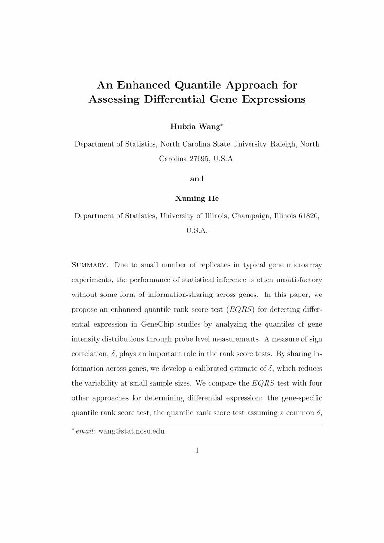
Summary. Due to small number of replicates in typical gene microarray
experiments, the performance of statistical inference is often unsatisfactory
without some form of information-sharing across genes. In this paper, we
propose an enhanced quantile rank score test (EQRS) for detecting differ-
ential expression in GeneChip studies by analyzing the quantiles of gene
intensity distributions through probe level measurements. A measure of sign
correlation, δ, plays an important role in the rank score tests. By sharing in-
formation across genes, we develop a calibrated estimate of δ, which reduces
the variability at small sample sizes. We compare the EQRS test with four
other approaches for determining differential expression: the gene-specific
quantile rank score test, the quantile rank score test assuming a common δ,
∗email: [email protected]
1

a modified t-test using summarized probe set level intensities, and the Mack-
Skilings rank test on probe level data. The proposed EQRS is shown to
be favorable for preserving false discovery rates and for being robust against
outlying arrays. In addition, we demonstrate the merits of the proposed
approach using a GeneChip study comparing gene expression in the livers
of mice exposed to chronic intermittent hypoxia and of those exposed to
intermittent room air.
Key words: GeneChip microarray; Probe level measurement; Quantile
regression; Rank score test; Information-sharing.
2

1. Introduction
In microarray studies, the number of replicates for each gene is generally
small. Statistical tests for detecting the differentially expressed genes, if per-
formed gene by gene, could suffer from low power or high false positive rates
due to unstable estimation of certain nuisance parameters such as variance
and correlation. Information-sharing across the genes, when utilized appro-
priately, often results in better genome-wide inference.
The idea of borrowing information across genes has been used in various
forms to assist inference. Baldi and Long (2001) proposed a regularized
t-test by using a pooled variance estimator, which combines the empiri-
cal variance with a local background variance associated with neighboring
genes. Lonnstedt and Speed (2002) proposed an empirical Bayes method by
using the information from all the genes to estimate the hyperparameters.
Storey and Tibshirani (2003) developed the SAM (Significance Analysis of
Microarray) t-test, which adjusts the gene-specific t-test by adding a positive
constant to the denominator of the t-statistic. Cui et al. (2005) developed a
shrinkage estimator of error variance using both the gene-specific variances
and some information across genes. Discussions on information-sharing can
also be found in Storey (2007) and Yang and Churchill (2007).
The present paper models the probe level GeneChip data. A number
of other authors have advocated the use of probe level data. For example,
Liu et al. (2006) adopted a Bayesian approach, using the probe level data
to obtain the summarized probe set expressions as well as their variabilities
(see Liu et al., 2005 for details), and then using them to compute the pos-
terior probability of up/down regulation. Lemieux (2006) used the probe
3

level data to directly estimate the treatment effects, followed by a mixture
model to cluster genes. Barrera et al. (2004) used a nonparametric test
based on ranks of probe level measurements. The cluster approach to detect
differentially expressed genes is not an inferential method, instead it relies
on visual inspection of the clusters. The Bayesian approach makes specific
parametric assumptions on various parts of the model, including Gaussian
errors. Furthermore, Liu et al. (2005) models correlation within each probe
pair, but like the rank test used by Barrera et al. (2004), it does not account
for the correlation among the probe level measurements on the same array in
deriving the variance estimates. The aforementioned probe level approaches
are mainly for screening, but less suited for inference that aims to have a
quantitative control for false positives. Wang and He (2007) developed a
rank score test for linear quantile models with a random effect to account
for intra-array correlation, and showed that the quantile rank score test is
more robust than the inference on the mean change (e.g., the t-tests) as it
accommodates a wide class of error distributions, including those with heavy-
tails. The small sample performance of the quantile rank score test depends
quite heavily on how a measure of intra-array sign correlation δ is estimated.
Wang and He (2007) considered using a genome-wide δ, estimated from all
the genes in the same experiment. This approach hinges on the belief that
the true δ varies slightly from gene to gene. While the majority of genes tend
to show consistency in their δ values, some interesting genes may violate this
constancy. In this paper, we aim to improve on the common δ approach in
the quantile rank score test and propose a new method to calibrate δ estima-
tion by sharing information across the “interesting” genes. The calibrated
4

value δ shrinks the gene-specific estimate δ towards a common value, with
the degree of shrinkage depending on how δ compares with those of some
other genes.
The detail of the enhanced quantile rank score test is given in Section
2. We use a simulation study to show that the proposed test performs well
and is superior to the Mack-Skillings test considered in Barrera et al. (2004)
for controlling false discovery, and to the modified SAM t-test based on
the summarized probe set level data, a commonly used microarray analysis
package developed by Storey and Tibshirani (2003), for handling outlying
observations. In Section 4, the proposed approach is applied to the Obese
Mice study, conducted by the Department of Medicine at Johns Hopkins Uni-
versity, and designed to study the effects of chronic intermittent hypoxia on
gene expression in the liver of leptin-deficient obese mice. Our investigation
indicates that our proposed analysis is more robust and powerful than the
SAM t-test in detecting differentially expressed genes, and it is more infor-
mative than the common δ approach. We provide some concluding remarks
in Section 5.
2. Enhanced Quantile Rank Score Test
We focus on detecting differentially expressed genes using the probe level data
in GeneChip studies. The intensity measures are assumed to have been pre-
processed with appropriate background correction and normalization. We
start this section with a review of the quantile rank score test in this context.
5

2.1 Quantile Rank Score Test
Suppose the total number of genes is G. We consider the following gene-
specific linear model
yijk = µ + Ti + Pk + uijk, i = 1, · · · , I, j = 1, · · · , J, k = 1, · · · , K, (1)
where yijk is the logarithm transformed intensity measurement for probe k
of the given probe set in array j under treatment i, µ is the overall level, Ti
is the effect of treatment i, Pk is the effect of probe k, and uijk = aij + eijk
are the composite error terms with aij representing the i.i.d. random effects
and eijk the random errors. The total number of measurements is n = IJK.
Following the linear model convention, we use X = (xijk) to denote the
n × p design matrix for the probe effects with the first column as 1, and
Z = (zijk) to denote the n× q design matrix for the treatment effects, where
p = K and q = I − 1 for Model (1). In more general settings, X may
include additional covariates with p > K. With this in mind, we consider a
partitioned linear mixed model
yijk = xTijkα + zT
ijkβ + uijk, 1 ≤ i ≤ I, 1 ≤ j ≤ J, 1 ≤ k ≤ K, (2)
where β ∈ Rq, the treatment effect size, is of primary interest. We consider
the problem of testing the null hypotheses H0 : β = 0.
Let ρτ (u) = u · {τ − I(u < 0)} be the quantile loss function (Koenker,
2005), and its associated score function ψτ (u) = τ − I(u < 0). For any given
0 < τ < 1, we consider the τth quantile of y given (x, z), assuming that
the τth conditional quantile of u is zero for identifiability. By adapting to a
measure of sign correlation δ = P (u111 < 0, u112 < 0) in the model, Wang
6

and He (2007) used the quantile rank score test statistic
Tn(τ) = STn Q−1
n (δ)Sn, (3)
where
Sn = n−1/2∑
ijk
z∗ijkψτ (uijk),
uijk = yijk − xTijkα, α = argmin
∑
ijk
ρτ (yijk − xTijkα),
Qn(δ) = n−1∑
ijk
z∗ijkz∗Tijkτ(1− τ) + n−1
∑ij
∑
k1 6=k2
z∗ijk1z∗Tijk2
(−τ 2 + δ),
δ = (n− p)−1∑ij
∑
k1 6=k2
I(uijk1 < 0, uijk2 < 0),
z∗ijk are the residuals from regressing Z on X, and I(·) is the indicator func-
tion. As J goes to infinity, Wang and He (2007) established the chi-square
limiting distribution of Tn, and showed the consistency of δ under H0.
2.2 Local Alternatives
It is helpful to consider the behavior of Sn under the local alternative
Hn : β = β0n−1/2 for some fixed β0. For this purpose, let F1 be the common
marginal distribution function of uijk, and F1,2 the joint distribution function
of uijk1 and uijk2 for any i, j and k1 6= k2. Assume that F1 has a Lebesgue
density f1 > 0 with a bounded first-order derivative, and that F1,2 is Lipschitz
in a neighborhood of (0, 0) with a second-order partial derivative f1,1 = f2,2
and a second-order mixed derivative f1,2. Also, let D1 = n−1Z∗T Z∗, and
D2 = n−1XT X.
Given the regularity conditions (A2) – (A4) of Wang and He (2007), we
can obtain, with routine modifications to Theorem 3.3 of He and Shao (1996),
7

the following Bahadur representation under Hn,
α− α = n−1D−12 {f1(0)}−1
{∑
ijk
xijkψτ (uijk)
}
+ n−1/2(XT X)−1XT Zβ0 + Op(n−3/4(loglogn)3/4), (4)
Following similar arguments to those in Lemma 2.2.2 of Wang and He (2007),
we see that under Hn, Sn has the same asymptotic distribution as
S∗n = n−1/2∑
ijk
z∗ijkψτ (yijk − xTijkα) = n−1/2
∑
ijk
z∗ijkψτ (uijk + n−1/2z∗Tijkβ0).
It then follows from the Lindberg-Feller central limit theorem that
Sn = AN (D1f1(0)β0, Qn(δ)) . (5)
Furthermore, by expanding F1,2 around (0, 0) and collecting the terms in-
volving β0, we obtain
δ − δ = cn + n−1f1,1(0, 0)
{n−1
∑
ijk
(z∗Tijkβ0)2
}
+n−1f1,2(0, 0)
{L−1
∑ij
∑
k1 6=k2
(z∗Tijk1β0)(z
∗Tijk2
β0)
}+ op(n
−1), (6)
where cn = O(n−1/2) is a term that is free of β0. For comparison between
two treatment groups, we have q = 1, z∗1jk = 1 and z∗2jk = −1. By (6), we
have
δ − δ = cn + dn−1β20 + op(n
−1), (7)
where d = f1,1(0, 0) + f1,2(0, 0).
Now consider a total number of G genes in the study. In what follows, we
shall use subscript g to denote the gene-specific values, and wish to test the
8

null hypotheses H0 : βg = 0 against the local alternative Hn : βg = n−1/2β0g,
where β0g is fixed, g = 1, · · · , G. Only the case of q = 1 will be considered in
the remainder of this Section.
The expressions (5) and (7) suggest that Sn is linearly related to β0, but
the local bias δ−δ is quadratic in β0. Thus, we expect δ−δ to have a quadratic
relationship with |Sn|. This relationship may be verified empirically; see
Figure 1 for the plot of δ − δ with respect to |Sn| for a simulated data set
from Case 1 described in Section 3. This is the basis of our proposed method
for calibrating δ in the next subsection.
[Figure 1 about here.]
2.3 Calibration of δ and the Proposed Test
To motivate our proposed method, we make the working assumption that
δg is normally distributed, and δg is approximately normal (c.f., the central
limit theorem). Following the discussion in Section 2.2, we use the approxi-
mating models as follows:
δg|µ, θ2 ∼ N(µ, θ2), (8)
δg|δg, Λ, H0 ∼ N(δg, σ2), (9)
and
δg|δg, Sng, Λ, Hn ∼ N(δg + a + bS2ng, σ
2), (10)
where Λ = (a, b, µ, σ, θ) denotes the hyperparameters. Direct calculations
show
δg|Λ, H0 ∼ N(µ, σ2 + θ2), (11)
δg|Sng, Λ, Hn ∼ N(µ + a + bS2ng, σ
2 + θ2), (12)
9
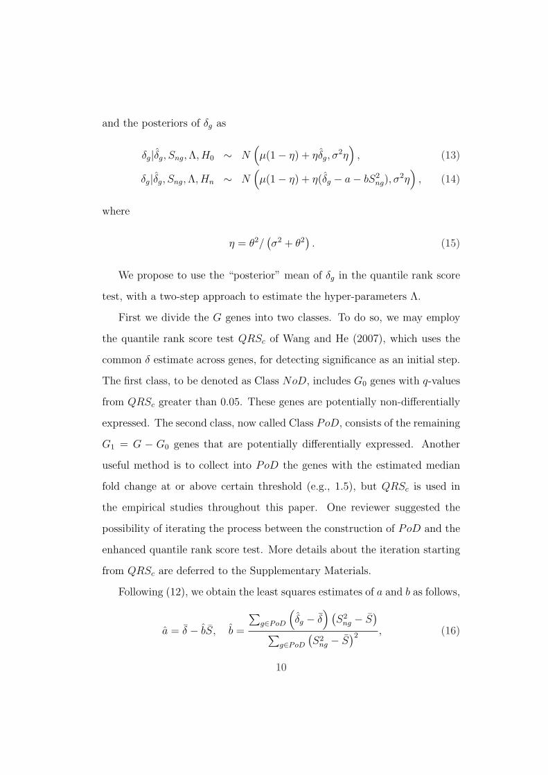
and the posteriors of δg as
δg|δg, Sng, Λ, H0 ∼ N(µ(1− η) + ηδg, σ
2η)
, (13)
δg|δg, Sng, Λ, Hn ∼ N(µ(1− η) + η(δg − a− bS2
ng), σ2η
), (14)
where
η = θ2/(σ2 + θ2
). (15)
We propose to use the “posterior” mean of δg in the quantile rank score
test, with a two-step approach to estimate the hyper-parameters Λ.
First we divide the G genes into two classes. To do so, we may employ
the quantile rank score test QRSc of Wang and He (2007), which uses the
common δ estimate across genes, for detecting significance as an initial step.
The first class, to be denoted as Class NoD, includes G0 genes with q-values
from QRSc greater than 0.05. These genes are potentially non-differentially
expressed. The second class, now called Class PoD, consists of the remaining
G1 = G − G0 genes that are potentially differentially expressed. Another
useful method is to collect into PoD the genes with the estimated median
fold change at or above certain threshold (e.g., 1.5), but QRSc is used in
the empirical studies throughout this paper. One reviewer suggested the
possibility of iterating the process between the construction of PoD and the
enhanced quantile rank score test. More details about the iteration starting
from QRSc are deferred to the Supplementary Materials.
Following (12), we obtain the least squares estimates of a and b as follows,
a = δ − bS, b =
∑g∈PoD
(δg − δ
) (S2
ng − S)
∑g∈PoD
(S2
ng − S)2 , (16)
10

where δ = G−11
∑g∈PoD δg and S = G−1
1
∑g∈PoD S2
ng.
Considering the distribution of δg|(Λ, H0), we choose the estimates of µ
and θ2 + σ2, respectively as,
µ =1
G0
∑g∈NoD
δg, and s2 =1
G0
∑g∈NoD
(δg − µ
)2
. (17)
To estimate σ2, we use
σ2 =1
G
G∑g=1
V ar(δg|δg). (18)
For each gene g, V ar(δg|δg) may be approximated by the large sample theory,
but we find it more stable to estimate it through bootstrap. First we resample
the estimated residuals by treating arrays as exchangeable units. We regress
the bootstrapped y values on X to obtain the bootstrap estimate δ∗g . Then
V ar(δg|δg) is estimated by the sample variance of δ∗g over 500 bootstrap
samples. Based on (15), (17) and (18), we estimate θ2 and η respectively by
θ2 = max (s2 − σ2, 0), and η = θ2/s2. (19)
Therefore, the posterior mean of δg can be estimated as
δg = µ(1− η) + ηδg, g ∈ NoD, (20)
and
δg = µ(1− η) + η max(τ 2, δg − a− bS2ng), g ∈ PoD, (21)
where the lower floor of τ 2 in max(τ 2, δg − a− bS2ng) above is based on our
assumption of positive correlation within arrays.
11

Finally, we define the enhanced quantile rank score test statistic as
Tng(τ) = S2ng/Qng(δg). (22)
The hypothesis testing can then be carried out using the χ21 distribution on
Tng(τ), and the test will be referred to as EQRS.
The calibrated δg shrinks the estimated δg towards the common value µ.
The degree of shrinkage depends on the variation of δ and that of δ. Note
that when the true δ is a constant, we have θ = 0 and δg = µ, and as a result,
we are shrinking δ to a common value and the EQRS reduces to QRSc of
Wang and He (2007).
3. Monte Carlo Simulations
We conduct a simulation study to investigate the performance of the quantile
rank score test QRS0 and two “information-sharing” quantile approaches
QRSc and EQRS. The two simpler tests QRS0 and QRSc were used in
Wang and He (2007). For comparison, we also perform two other tests for
gene detection. One is the Mack-Skillings rank-based test (MS) on two-way
ANOVA, as suggested in Barrera et al. (2004), which acts on probe level
data. The other is the SAM t-test (Storey and Tibshirani, 2003) based
on RMA (Robust Multi-array Average, Irizarry et al., 2003) summarized
intensity measurements, which will be called RMA+SAM in the paper, and
is carried out with Bioconductor’s affy package for RMA and samr for SAM
(with the default setting as of August, 2006).
The simulation study is based on Model (1) with I = 2 and K = 16, which
mimics a GeneChip experiment to identify differential expressions between
12

two groups, and uijk = aij + eijk, where aij is the jth random array effect
nested within the ith treatment, and eijk is the random error. We assume
that each treatment has J replicate arrays. The parameter β = T1 − T2
measures the treatment effect. The rank score tests focus on the median
regression (τ = 0.5) in this simulation study with four cases. A fifth case
that mimics the Obese Mice data analyzed in Section 4 is reported in the
online Supplementary Materials.
In Case 1, the aij’s and eijk’s are generated from N(0, σ2A) and N(0, σ2
e),
respectively, where σA is chosen to be 0.2 and kept unchanged, σ2e is set
to be σ2A(1 − γ)/γ, and γ = σ2
A(σ2A + σ2
e)−1 is the intra-array correlation
coefficient and varies from gene to gene. The γ’s are generated by converting
the Fisher’s z, which are randomly chosen from N(0.2, 0.12), back to the
correlation scale. For the particular z generated, the range of the theoretical
δ is [0.25, 0.32]. The settings in Case 2 are the same as in Case 1 except that
the Fisher’s z is generated from N(0.2, 1), resulting in a wider range [0.25,
0.50] for δ. To study the robustness of each method to outlying observations,
we perturb the data generated in Case 2 by subtracting 2T1 from a11 in Case
3, and by subtracting 2 from the first 5 probes in the first 2 arrays in Case
4. Case 3 mimics the situation where an outlying array in one group reduces
the difference between groups. For a real example in this situation, see gene
1417389 at studied in Section 4 (Figure 3). Case 4 mimics the scenario of
outlying probes that result in a large variation between replicate arrays. Our
experience indicated that these two scenarios were not rare in GeneChip
experiments.
To examine the true positives and false positives associated with each test,
13

we simulate 100 data sets in each case. Each data set consists of 3,000 genes,
of which 2,500 genes are non-differentially expressed (β = 0) and 500 genes
are differentially expressed (β drawn from the standard normal distribution
N(0, 1)). For each gene, the probe effects Pk are generated from N(0, 22)
independently, and they are held constant across all the simulations. Three
values J =5, 7 and 10 are used.
For each simulated data set, the q-values under QRS0, QRSc, EQRS and
MS are calculated following Storey (2002), and the q-values of RMA+SAM
are estimated from the permutation method implemented in samr. Table 1
summarizes the results in terms of true positives and false positives, where
TP is the number of detected genes which are truly differentially expressed,
FP is the number of falsely detected genes, and FDR is the ratio of the total
number of false positives to the total number of detected genes, averaged
across the 100 simulated data sets. The FDR for a given data set is taken
as 0 when no gene is detected.
[Table 1 about here.]
Since the MS test does not account for the intra-array correlation in
the probe level data, it leads to seriously inflated FDR, which reaffirms the
need to treat the array effect as random in our study. As observed in Wang
and He (2007), QRS0 loses some power at small samples, but it performs
competitively for moderate samples sizes (J ≥ 10). The QRSc performs
better than QRS0 at small samples when the true δ vary slightly across
genes (e.g., J = 5 in Case 1), but it loses some control of FDR in Cases
2–4 where δ vary extensively. The proposed EQRS controls FDR around
14

5% reasonably well (except in Case 3 with J = 5 where the FDR is not
as meaningful due to a very small number of “discoveries”), and has better
overall performance than QRS0. The RMA+SAM approach is very sensitive
to outlying observations. More specifically, it loses power to detect in Case
3, while it provides seriously inflated FDR in Case 4.
To compare the sensitivity and specificity of different methods, we look
at the Receiver Operator Characteristic (ROC) curves. The ROC curve in
Figure 2 plots the true positives TP against the false positives FP , averaged
across the 100 simulated data sets, up to a maximum of 100 FP ’s obtained
at each possible threshold value. For easier interpretation, we use the TP
and FP instead of true positive and false positive rates in the figure. All five
methods give similar ROC curves in Cases 1, 2 and 4, but the quantile rank
score tests, especially those with information-sharing, are clearly better than
the RMA+SAM approach in Case 3.
[Figure 2 about here.]
4. Empirical Data Analysis
We apply QRSc, EQRS, RMA+SAM and MS to an Obese Mice study to
assess their real world performances. The results from the Bayesian approach
of Liu et al. (2006) are not easily compared with those from our approach.
Differences in the approaches include differences in data preprocessing (back-
ground adjustment and normalization). More importantly, it is unclear on
how to control FDR based on the posterior probabilities of up-regulation (or
down-regulation) returned from the Bayesian method. Even though the com-
parison of EQRS to the Bayesian approach is not the focus of our study, the
15

analysis results on the Obese Mice data and some discussions are provided
as part of the online Supplementary Materials.
The Obese Mice study was conducted by the Department of Medicine at
Johns Hopkins University. The raw data sets can be downloaded from the
National Center for Biotechnology Information (accession no. GSE1873).
The experiment was designed to study the effects of chronic intermittent
hypoxia (CIH) on gene expression in the liver of leptin-deficient obese mice.
Five mice were exposed to CIH and another five were exposed to intermittent
room air (IA, control condition) for 12 consecutive weeks. The liver cRNA
from each sample was hybridized to Affymetrix 430A 2.0 GeneChip array,
producing a total of 10 arrays. More information of the data set can be found
in Li et al. (2005). The number of genes analyzed is G = 22, 690, and the
number of probes is 11 for most of the genes. The data is preprocessed with
background correction and the quantile normalization using the R package
affy from Bioconductor. In this analysis, we focus on the rank score tests for
the median.
Following the procedures described in Section 2, we obtain the q-values
from each test, and identify the genes with q-values smaller than 0.05 as
differentially expressed. At the 5% FDR cutoff, the proposed EQRS de-
tects 30 genes, as compared to 37 genes detected by QRSc. The RMA+SAM
method is the least powerful one by detecting only 5 genes, all of which are
also identified by EQRS and QRSc. The Mack-Skillings test detects 2639
genes, nearly 2,000 of which have the estimated δ at 0.2 or higher, making
the MS-test overstate their significance in this example.
16

For a closer look, we give in Table 2 the summary statistics of 3 genes
missed by RMA+SAM. Figure 3 (a) and (c) show the box plots of probe level
intensities array by array for genes 1415822 at and 1417389 at, respectively.
The 5 shaded boxes represent the replicated samples exposed to IA, and the
other 5 boxes are of the samples exposed to CIH. Figure 3 (b) and (d) plot
the RMA summarized intensities. The solid dots are for IA and the open
circles are for CIH. For gene 1415822 at, even though the fold change is as
high as 3.8, the SAM t-test is not able to show significance mainly due to the
large variation between the five replicates of the CIH group. The EQRS at
the median gives q-value at 0.002. For gene 1417389 at, it is clear from both
Figure 3 (c) and (d) that IA is generally associated with higher intensities
than CIH. However, Array 2 from IA has lower intensities than the other
arrays under the same condition, which leads to the q-value of nearly 1 based
on the SAM t-test. These examples indicate loss of information when we
summarize the probe level measurements into a probe set level expression
index.
[Table 2 about here.]
[Figure 3 about here.]
To see the impact of calibration of δ in the median score tests, we use
Figure 4 (a) and (b) to plot δ and δ against |Sn| for genes with |Sn| > 1.500.
Here δ denotes the calibrated δ under EQRS. The horizontal dashed line
stands for the common δ estimate used in QRSc. From Figure 4 (a), it
is clear that δ tends to increase with |Sn|, and the δ’s may vary a bit at a
given value of |Sn|. The downward triangle in Figure 4 (a) and (b) is for gene
17

1417389 at. In this case, the calibrated δ is much smaller than δ, allowing the
EQRS to return a smaller q-value. The same holds true for gene 1415822 at.
Both genes are in the PoD class, so the calibrations based on (21) aim to
correct the bias in the δ due to larger values of |Sn|.
[Figure 4 about here.]
The upward triangle is of gene 1423418 at, which is identified as signifi-
cant by QRSc but not by EQRS. Among the genes with |Sn| = 1.573, gene
1423418 at still has a relatively large δ. The method QRSc simply ignores
this variation and shrinks all the δ’s to a common value, while the calibrated
δ takes this information into account by using a relatively large δ estimate
for this gene in the test statistic.
It is easy to argue that, when the alternative hypothesis is true, the
δ estimation obtained from the full-model residuals, referred to as δ1, is
generally more accurate than δ. Figure 4 (c) plots the δ’s (of those genes
with |Sn| = 1.573) against δ1. The plot suggests that δ is linearly related to
δ1, and that gene 1423418 at has an a larger δ1 than most others. Shrinking
this estimate of δ to a common value by QRSc has a clear risk of a false
positive for this gene, so the result from EQRS is more trustworthy. This is
further confirmed by looking at the δ1’s at the first quartile τ = 0.25 for the
same group of genes (Figure 4 (d)).
The Obese Mice study indicates that the quantile rank score test based
on probe level data is more robust and powerful than the SAM t-test based
on the summarized probe set level data. Following the procedure described
in Section 2, we obtain θ =0.0286 and µ = 0.2873 at the median. So the
18

coefficients of variation of δ is approximately 0.1, which is relatively high
compared to several other data sets that we have analyzed. In such circum-
stances, EQRS tends to be more reliable than QRSc.
5. Discussion and Conclusions
The quantile rank score test is a reliable inference method for detecting dif-
ferences in certain quantiles of the intensity distributions for the probe level
data. To better account for the within array correlation in the probe level
measurements, the proposed enhanced quantile rank score test EQRS is
shown to be more trustworthy than its gene-specific counterpart QRS0 and
the use of a genome-wide adjustment in QRSc, because the EQRS uses
a smart information-sharing approach to balance gene-specific information
with the commonality learned across the genes.
The calibration in EQRS is based on the observation that a measure
of sign correlation, δ, in the variance of the deviance Sn has a quadratic
relationship with the magnitude of Sn when local alternatives are true. We
derived a specific calibration method in the paper for testing the treatment
effect, but the idea can be extended to more general cases. For example, if
q > 1 in Model (2) as in multiple group comparison, we can approximate
the bias δ − δ by a quadratic function of bT Sn, where b is some q × 1 vector.
Although the extension to more general mixed models remains unclear at this
time, the proposed calibration idea can be applied not only to microarray
studies where many genes share the same model structure, but also to other
studies where the estimation of a certain nuisance parameter depends on part
of the test statistic.
19

Finally, we note that the empirical analysis on GeneChip data reported
in this paper used RMA for background correction and quantile normal-
ization, but the proposed EQRS retains its advantages when other data
pre-processing methods, such as the GCRMA of Wu et al. (2004), are used.
Supplementary Materials
The materials referenced in Section 2.3 and Section 3, as well as the R codes
used to analyze the Obese Mice data (Section 4) are available under the Paper
Information link at the Biometrics website http://www.tibs.org/biometrics.
Acknowledgements
The research is supported in part by NSF Awards DMS- 0706963 and DMS-
0604229. The authors are grateful to an Editor, an Associate Editor and a
referee for their helpful comments and suggestions.
References
Baldi, P. and Long, A. D. (2001). A Bayesian framework for the analysis of
microarray expression data: regularized t-test and statistical inferences of
gene changes. Bioinformatics 17, 509–19.
Barrera, L., Benner, C., Tao, Y. C., Winzeler, E., and Zhou, Y. (2004).
Leveraging two-way probe-level block design for identifying differential
gene expression with high-density oligonucleotide arrays. BMC Bioinfor-
matics 5:42, doi:10.1186/1471-2105-5-42.
20

Cui, X., Hwang, J. T., Qiu, J., Blades, N. J. and Churchill, G. A. (2005).
Improved statistical tests for differential gene expression by shrinking vari-
ance components estimates. Biostatistics 6, 59–75.
He, X. and Shao, Q. M. (1996). A general bahadur representation of M-
estimators and its application to linear regression with nonstochatic de-
signs. Annals of Statistics 24, 2608–2630.
Irizarry, R. A., Bolstad, B. M., Collin, F., Cope, L. M., Hobbs, B. and Speed,
T. P. (2003). Summaries of Affymetrix GeneChip probe level data. Nucleic
Acids Research 31, e15.
Koenker, R. (2005). Quantile regression. Cambridge University Press, Cam-
bridge, NY, USA.
Lemieux, S. (2006). Probe-level linear model fitting and mixture modeling
results in high accuracy detection of differential gene expression. BMC
Bioinformatics 7:391, doi: 10.1186/1471-2105-7-391.
Liu, X., Milo, M., Lawrence, N. D., and Rattray, M. (2005). A tractable
probabilistic model for Affymetrix probe-level analysis across multiple
chips. Bioinformatics 21(18): 3637-3644.
Liu, X., Milo, M., Lawrence, N. D., and Rattray, M. (2006). Probe-level
measurement error improves accuracy in detecting differential gene ex-
pression. Bioinformatics 22, 2107–21132.
Lonnstedt, I. and Speed, T. P. (2002). Replicated microarray data. Statistica
Sinica 12, 31–46.
Li, J., Grigoryev, D., Ye, S. Q., Thorne, L., Schwartz, A. R., Smith, P. L.,
O’Donnell, C. P. and Polotsky, V. Y. (2005). Chronic intermittent hypoxia
up-regulates genes of lipid biosynthesis in obese mice. Journal of Applied
21

Physiology 99, 1643–1648.
Storey, J. D. (2002). A direct approach to false discovery rates. Journal of
the Royal Statistical Society Series B 64, 479–498.
Storey, J. D. (2007). The optimal discovery procedure: A new approach to
simultaneous significance testing. Journal of the Royal Statistical Society
Series B 69, 347-368.
Storey, J. D. and Tibshirani, R. (2003). SAM thresholding and false discovery
rates for detecting differential gene expression in DNA microarrays. In
Parmigiani, G., Garrett, E. S., Irizarry, R. A. and Zeger, S. L., editors,
The Analysis of Gene Expression Data: Methods and Software, pages
272–289. New York, Springer.
Wang, H. and He, X. (2007). Detecting differential expressions in GeneChip
microarray studies: a quantile approach. Journal of American Statistical
Association 102, 104-112.
Wu, Z., Irizarry, R. A., Gentleman, R., Martinez-Murillo, F. and Spencer,
F. (2004). A Model-Based Background Adjustment for Oligonucleotide
Expression Arrays. Journal of the American Statistical Association 99,
909–917.
Yang, H. and Churchill, G. (2007). Estimating p-values in small microarray
experiments. Bioinformatics 23, 38–43.
22

0.0 0.5 1.0 1.5 2.0 2.5 3.0
−0.0
50.
000.
050.
100.
150.
20
|Sn|
δ−δ
Figure 1. The δ − δ against |Sn| from a simulated data set from Case 1described in Section 3.
23

0 10 20 30 40 50
010
020
030
040
0
Case 1, J=7
False Positives
True
Pos
itives
0 10 20 30 40 50
050
100
150
200
250
300
350
Case 3, J=7
False Positives
True
Pos
itives
QRS0 QRSc EQRS RMA+SAM MS
Figure 2. The ROC curves of QRS0, QRSc, EQRS, RMA+SAM and MSin Cases 1 and 3 at J = 7.
24

1 2 3 4 5 6 7 8 9 10
−2
−1
01
23
(a) Gene 1415822_at
Array
(b) Gene 1415822_at
Group
IA CIH
6.5
7.5
8.5
9.5
10
.5
1 2 3 4 5 6 7 8 9 10
−1
.0−
0.5
0.0
0.5
1.0
(c) Gene 1417389_at
Array
(d) Gene 1417389_at
Group
IA CIH
8.3
8.6
8.9
9.2
9.5
Figure 3. Expression profiles of genes 1415822 at and 1417389 at in theObese Mice study. In the left panel, the y-axis is the probe level log2(PM)centered at the probe-wise median of 10 arrays; the shaded boxes are for thesamples exposed to IA and the other 5 boxes are for the samples exposedto CIH. In the right panel, the y-axis is the RMA summarized probe setexpression value; the solid dots are 5 replicates of IA and the open circles are5 replicates of CIH.
25

1.6 1.8 2.0 2.2 2.4
0.25
0.30
0.35
0.40
0.45
0.50
(a) |Sn|>1.500
|Sn|
δ
1.6 1.8 2.0 2.2 2.4
0.25
0.30
0.35
0.40
0.45
0.50
(b) |Sn|>1.500
|Sn|δ~
0.30 0.35 0.40
0.25
0.30
0.35
0.40
0.45
0.50
(c) |Sn|=1.573
δ1
δ
0.06 0.08 0.10 0.12 0.14 0.16
0.25
0.30
0.35
0.40
0.45
0.50(d) |Sn|=1.573
δ1 at the first quartile
δ
Figure 4. Figures (a) and (b) plot δ and δ against |Sn| for genes with|Sn| > 1.500, where the horizontal dashed line stands for the common δ usedin QRSc. Figures (c) and (d) plot δ against δ1 at the median and at the firstquartile, respectively, for the genes with |Sn| = 1.573. The solid up-pointtriangle, the square and the down-point triangle denote genes 1423418 at,1415822 at and 1417389 at, respectively.
26

Table 1The number of true positives (TP), false positives (FP), and the estimatedfalse discovery rates (FDR) in Cases 1–4. The desired FDR is 0.05. When
very few genes are detected to be positive, the FDR is not estimated butrather indicated by *. The standard errors of the FDR estimates for the
quantile-based tests are within 0.02 in all the cases where TP > 1.
Case 1 Case 2 Case 3 Case 4J 5 7 10 5 7 10 5 7 10 5 7 10
QRS0
TP 232 320 358 294 337 369 0 0 335 273 329 365FP 1 8 13 9 13 17 0 0 15 8 15 19FDR 0.01 0.02 0.04 0.03 0.04 0.04 * * 0.04 0.03 0.04 0.05
QRSc
TP 302 328 354 315 337 356 0 294 336 300 331 356FP 10 11 12 39 28 28 1 25 27 37 31 31FDR 0.03 0.03 0.03 0.11 0.08 0.07 * 0.08 0.08 0.11 0.09 0.08
EQRSTP 309 338 362 307 345 371 0 291 343 294 338 367FP 13 15 16 15 23 23 1 23 23 20 24 23FDR 0.04 0.04 0.04 0.05 0.06 0.06 * 0.07 0.06 0.06 0.06 0.06
RMA+SAMTP 323 348 372 338 361 375 1 2 294 333 347 367FP 16 18 20 17 19 19 2 1 16 245 95 75FDR 0.05 0.05 0.05 0.05 0.05 0.05 * * 0.05 0.37 0.19 0.16
MSTP 417 429 441 446 458 463 417 438 451 440 450 460FP 532 534 543 1069 1076 1062 1067 1071 1059 1105 1095 1078FDR 0.56 0.55 0.55 0.71 0.70 0.70 0.72 0.71 0.70 0.72 0.71 0.70
27

Table 2Summary statistics of three genes in the Obese Mice study. The proposedmethod with information-sharing calibrates δ toward δ, Sn is the observed
quantile rank score and FC is the estimated fold change based on the RMAsummarized values (“−” for down-regulation and “+” for up-regulation).
q-valuesProbe Set QRSc EQRS SAM Sn δ δ FC
1415822 at 0.023 0.002 0.415 1.669 0.375 0.271 3.81417389 at 0.012 0.008 1.000 −1.764 0.399 0.288 −1.51423418 at 0.042 0.390 0.279 1.573 0.450 0.316 2.9
28