BUSINESS GROWTH STRATEGIES OF ILLINOIS FARMS: A QUANTILE

REGRESSION APPROACH

Enrique Hennings and Ani L. Katchova

Selected Paper prepared for presentation at the American Agricultural Economics Association Annual Meeting, Providence, Rhode Island, July 24-27, 2005

Contact Information: Ani L. Katchova University of Illinois at Urbana-Champaign 326 Mumford Hall, MC-710 1301 West Gregory Drive Urbana, IL 61801 Tel: (217) 333-7760 Fax: (217) 333-5538 E-mail: katchova@uiuc.edu

Enrique Hennings University of Illinois at Urbana-Champaign 326 Mumford Hall, MC-710 1301 West Gregory Drive Urbana, IL 61801 Tel: (217) 359 1499 E-mail: emhennin@uiuc.edu

Enrique Hennings is a PhD student and Ani L. Katchova is an assistant professor in the Department of Agricultural and Consumer Economics at the University of Illinois at Urbana-Champaign. Copyright 2005 by Enrique Hennings and Ani L. Katchova. All rights reserved. Readers may make verbatim copies of this document for non-commercial purposes by any means, provided that this copyright notice appears on all such copies.

2

Business Growth Strategies of Illinois Farms: A Quantile Regression Approach

This study examines the business strategies employed by Illinois farms to maintain equity

growth using quantile regression analysis. Using data from the Farm Business Farm

Management system, this study finds that the effect of different business strategies on

equity growth rates differs between quantiles. Financial management strategies have a

positive effect for farms situated in the highest quantile of equity growth, while for farms

in the lowest quantile the effect on equity growth is negative. Cost reduction, asset

management and revenue enhancement strategies all proved to have important effects on

the determination of growth equity rates.

Key words: business growth, equity growth, percentile, quantile regression.

1

Business Growth Strategies of Illinois Farms: A Quantile Regression Approach

The 1996 Farm Bill dismantled an income support mechanism that U.S. farmers

had enjoyed since 1973, resulting in a high income volatility period for the farm sector.

The federal government disbursed billons of dollars to stabilize farm income. Farmers

received $4.3 billion in direct government payments in 1997, $6.0 billion in 1998, and

$8.7 billion in 1999 (ERS-USDA). In 1997, the average large family farm recipient

received over $18,000 in benefits. Illinois farmers received federal support above

national average; however the government efforts were not enough to stabilize income

variability. As a reaction, Illinois farms have adopted several business strategies to avoid

the deterioration of their equity positions. Among the strategies that have been adopted

by Illinois farms are asset management, financial management, revenue enhancement,

and cost reduction strategies.

Previous studies have looked at the effect that these strategies have had on the

equity positions of Illinois farms. In particular, Escalante and Barry (2002) identified key

strategies employed by Illinois grain farms to prevent deterioration of their equity growth

after the 1996 Farm Bill. Using an OLS regression with farm data, they identified that

revenue enhancement, cost reduction and capital management strategies were important

to maintain equity level. By pooling all farms together and estimating a mean based

regression (OLS), Escalante and Barry (2002) overlooked the possibility that farms at

different points in the distribution of equity growth may actually face different effects

from the same strategies.

2

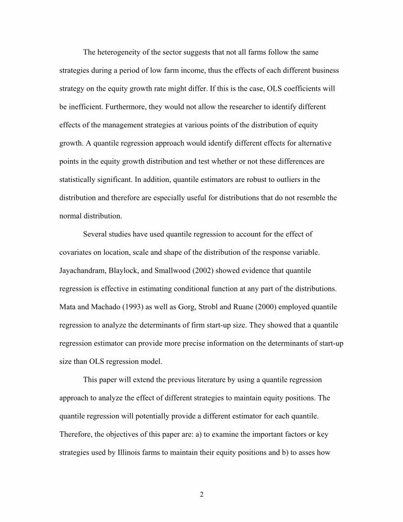
The heterogeneity of the sector suggests that not all farms follow the same

strategies during a period of low farm income, thus the effects of each different business

strategy on the equity growth rate might differ. If this is the case, OLS coefficients will

be inefficient. Furthermore, they would not allow the researcher to identify different

effects of the management strategies at various points of the distribution of equity

growth. A quantile regression approach would identify different effects for alternative

points in the equity growth distribution and test whether or not these differences are

statistically significant. In addition, quantile estimators are robust to outliers in the

distribution and therefore are especially useful for distributions that do not resemble the

normal distribution.

Several studies have used quantile regression to account for the effect of

covariates on location, scale and shape of the distribution of the response variable.

Jayachandram, Blaylock, and Smallwood (2002) showed evidence that quantile

regression is effective in estimating conditional function at any part of the distributions.

Mata and Machado (1993) as well as Gorg, Strobl and Ruane (2000) employed quantile

regression to analyze the determinants of firm start-up size. They showed that a quantile

regression estimator can provide more precise information on the determinants of start-up

size than OLS regression model.

This paper will extend the previous literature by using a quantile regression

approach to analyze the effect of different strategies to maintain equity positions. The

quantile regression will potentially provide a different estimator for each quantile.

Therefore, the objectives of this paper are: a) to examine the important factors or key

strategies used by Illinois farms to maintain their equity positions and b) to asses how

3

different strategies affect farms according to their position on the equity growth

distribution. This will allow us to evaluate the relative importance of the strategies at different

points of the distribution of farms’ equity growth.

The following sections present the methodology and model specifications, the

econometric analysis as well as a description of the data and the regression results.

Methodology and Model Specification

This section outlines the methodology employed to construct the variables

considered in the study. It includes the description of the theoretical model as well as the

econometric models employed during the analysis. Barry et al. (2001) define equity

growth according to the following equation:

(1) [ ] [ ]g r *(A / E) i * (D / E * (1 t) *(1 c)= − − −

where r is the expected rate of return on assets, A/E is the asset to equity ratio, i is the

cost of debt, D/E is the debt to equity ratio, t is the net withdrawals for taxation and c is

the family consumption. Equation (1) shows how the rate of equity growth is influenced

by several factors. If the rate of return on assets or the asset to debt ratio were to

increase, the rate of equity growth would increase as well. On the other hand, as the rate

of interest rate, taxation and consumption increase, the rate of equity growth will

decrease. These alternative strategies that influence the rate of equity growth have been

classified into four major categories: asset management, financial management, revenue

enhancement, and cost reduction (Escalante and Barry, 2002). The following paragraphs

describe in detail these strategies.

4

Asset Management Strategies

The asset management strategy refers to the optimization of rate of return on assets

through either revenue enhancement or cost reduction. It indicates whether or not the

utilization of farm assets translates to favorable high returns for the farm business. When

a farm chooses the adequate level of asset either by selling or buying assets, the

productivity ratios can be improved leading to a better equity position.

Financial Management Strategies

Financial management strategies refer primarily to debt and equity management

strategies. They may entail the regulation of the debt to equity rate and borrowing costs

such as interest paid by the farm. Financial management strategies try to minimize the

financial stress of farms therefore the adequate level of debt can stimulate equity growth.

If the cost of borrowing exceeds the farm returns, higher level of leverage will translate in

a deterioration of the farm’s equity position

Revenue Enhancement Strategies

These strategies aim to enhance the net contribution of farm activities and to increase the

farm net worth. The revenues of the farm can be enhanced by identifying existing assets

that are not generating as much revenue as they might, developing marketing plans

backed by thorough financial resources, analysis, and hedging brokerage relations.

Cost Reduction

Cost reduction strategies refer to cost control strategies that improve the operation

efficiency. They might include the selection of cost effective technologies and inputs,

cost saving production scheduling, and other overhead cost reduction schemes (Escalante

and Barry, 2002).

5

Following Escalante and Barry (2002), ten variables are chosen to represent these

four alternative strategies to explain the rate of equity growth. Therefore the equity

growth is defined as follow:

Equity growth = f (asset turnover, tenure, share leasing ratio, leverage,

interest expenses ratio, net farm income ratio, off-farm income, operating

expenses ratio, family living expenses)

Equity growth is defined as the annual change in farm equity capital. The change

in equity reflects the effect of retained earnings, realized capital gains on non-real state

assets as well as the unrealized nominal capital gain on farm real state. Since the original

purchase value of farmland is difficult to identify from the FBFM data base, the equity

growth rate was adjusted by eliminating the contribution from unrealized capital gains on

farmland thus obtaining the realized equity growth. This adjustment consists on

subtracting to the farm equity capital on year t the acreages own by the farm in the

previous year (t-1) multiplied by the change in farmland value.

The asset turn over ratio, the tenure ratio and the share leasing ratio correspond to

the asset management strategy. The asset turn over ratio is calculated by dividing the

value of farm production by the value of total farm assets and measures how efficiently

farm assets are being used to generate revenue. A farm business has two ways to

increase profits – either by increasing the profit per unit produced or by increasing the

volume of production (if the business is profitable). A relationship exists among the rate

of return on farm assets, the asset turnover ratio, and the operating profit margin ratio.

The higher the asset turn over ratio, the more efficiently assets are being used to generate

6

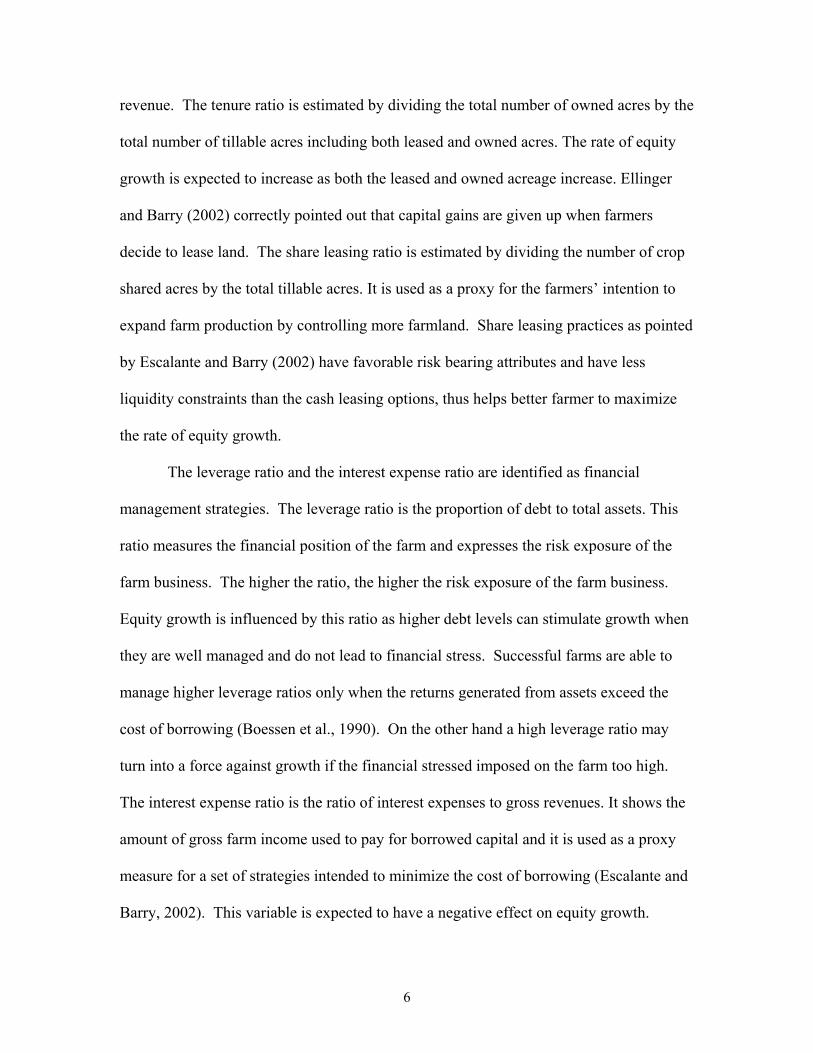
revenue. The tenure ratio is estimated by dividing the total number of owned acres by the

total number of tillable acres including both leased and owned acres. The rate of equity

growth is expected to increase as both the leased and owned acreage increase. Ellinger

and Barry (2002) correctly pointed out that capital gains are given up when farmers

decide to lease land. The share leasing ratio is estimated by dividing the number of crop

shared acres by the total tillable acres. It is used as a proxy for the farmers’ intention to

expand farm production by controlling more farmland. Share leasing practices as pointed

by Escalante and Barry (2002) have favorable risk bearing attributes and have less

liquidity constraints than the cash leasing options, thus helps better farmer to maximize

the rate of equity growth.

The leverage ratio and the interest expense ratio are identified as financial

management strategies. The leverage ratio is the proportion of debt to total assets. This

ratio measures the financial position of the farm and expresses the risk exposure of the

farm business. The higher the ratio, the higher the risk exposure of the farm business.

Equity growth is influenced by this ratio as higher debt levels can stimulate growth when

they are well managed and do not lead to financial stress. Successful farms are able to

manage higher leverage ratios only when the returns generated from assets exceed the

cost of borrowing (Boessen et al., 1990). On the other hand a high leverage ratio may

turn into a force against growth if the financial stressed imposed on the farm too high.

The interest expense ratio is the ratio of interest expenses to gross revenues. It shows the

amount of gross farm income used to pay for borrowed capital and it is used as a proxy

measure for a set of strategies intended to minimize the cost of borrowing (Escalante and

Barry, 2002). This variable is expected to have a negative effect on equity growth.

7

The revenue enhancement strategy is represented by the net farm income and the

off-farm income. The net farm income ratio is obtained by dividing the net farm income

by the gross revenues. This variable is used to measure farmer’s actions to increase the

farm equity. To enhance farm revenues, Escalante and Barry (2002) point out the fact that

farmers can rely on alternative farm revenue enhancement strategies such as federal

income subsidy support, effective market strategies, and nontraditional uses of farm

products. Another proxy for revenue enhancement strategies is the off farm income.

Many farm families already have at least one family member earning supplemental

income away from the farm. An off-farm income source may not only generate steady

income for family expenses but can also help relieve the pressure of cash withdrawals

over the business profitability. Both variables are expected to have a positive impact on

equity growth.

The operating expense ratio and family living expenses are used as proxies for the

cost reduction strategy. The operating expenses ratio measures how efficiently the farm

business controls its operating expenses, and is calculated by dividing total operating

expenses by gross revenues. It indicates the proportion of farm income used to pay

operating expenses not including principal or interest. The equity growth ratio is expected

to be affected negatively as the operating expense ratio increases. The family living

expenses are cash withdrawals paid by the business to cover family living expenses. In

the context of the farming operation, family living withdrawals can be viewed as

compensation for the owner/operator's management and labor. Actual withdrawals in

excess of the amount needed to cover family living expenses can affect the equity growth

negatively especially for less profitable farms.

8

Econometric Models

Two econometric models are employed in this study. The first is an ordinary least squares

estimation (OLS) and the second is a quantile regression. Koenker and Basssett (1978)

introduced quantile regression as a generalization of sample quantiles to conditional

quantiles expressed as a function of explanatory variables. The quantile regression is an

extension of the OLS regression model that allows the specification of conditional

functions at any quantile. The quantile regression allows examining whether the effect of

a particular explanatory variable on equity growth differs by the position of the farm

business on the equity growth distribution. The quantile regression describes the entire

conditional distribution of equity growth given a set of asset management, financial

management, revenue enhancement, and cost reduction strategies. OLS regressions

impose the constraints that the effect of a particular explanatory variable on equity

growth is the same for the different equity growth groups. When the farms are

homoskedastic in term of growth on equity, the slope estimates of the conditional

quantile functions at each point of the distribution of the dependent variable will be equal

to each other and to the slope estimates from the OLS. However, when the farms are

hetersokedastic, the slope estimates of the conditional quantile functions will differ from

each others as well as from the OLS slope estimates. Therefore, estimating conditional

quantiles at various points of the distribution of the dependent variable will allow us to

trace out different marginal responses of the dependent variable to changes in the

explanatory variables at these points. Moreover, under the assumption of independently

and normally distributed errors, the estimator from the quantile regression may be more

9

efficient than the OLS estimators (Koenker and Basssett, 1978). The quantile regression

is also robust for outliers.

Buchinsky (1998) describes the general quantile regression model as follows:

(2) i i iy x ' u , i 1......n,θ θ= β + =

where yi denotes the equity growth for farm i and the θth quantile (0<θ<100) of the

conditional distribution of yi is a linear function of a K*1 vector of explanatory variables

xi and an unknown error term, uθi. ; βθ is the unknown vector of regression parameters

associated with the θth percentile. The conditional quantile function can be expressed

as θθ β')( iii xxyQ = . Thus the quantile regression estimator θβ̂ can be found as the solution

to the following minimization problem:

(3) ' '

i i i

' 'i i i i

y x yi xM in y x (1 ) y x

θθ θ

θ θβ ≥ β < β

θ − β + − θ − β

∑ ∑

The study considers nine quantile regressions at the 10th, 20th, 30th, 40th, 50th, 60th, 70th,

80th and 90th quantiles. To obtain a consistent estimator of the covariance matrix, it is

necessary to employ a design matrix bootstrap estimation (Jayachandram, 2002). In the

design matrix bootstrap estimation, the quantile regression is estimated with sample of N

observations drawn randomly with replacement from the original sample. For this study,

the method was repeated 1000 times to obtain bootstrap estimates θβ̂ .

10

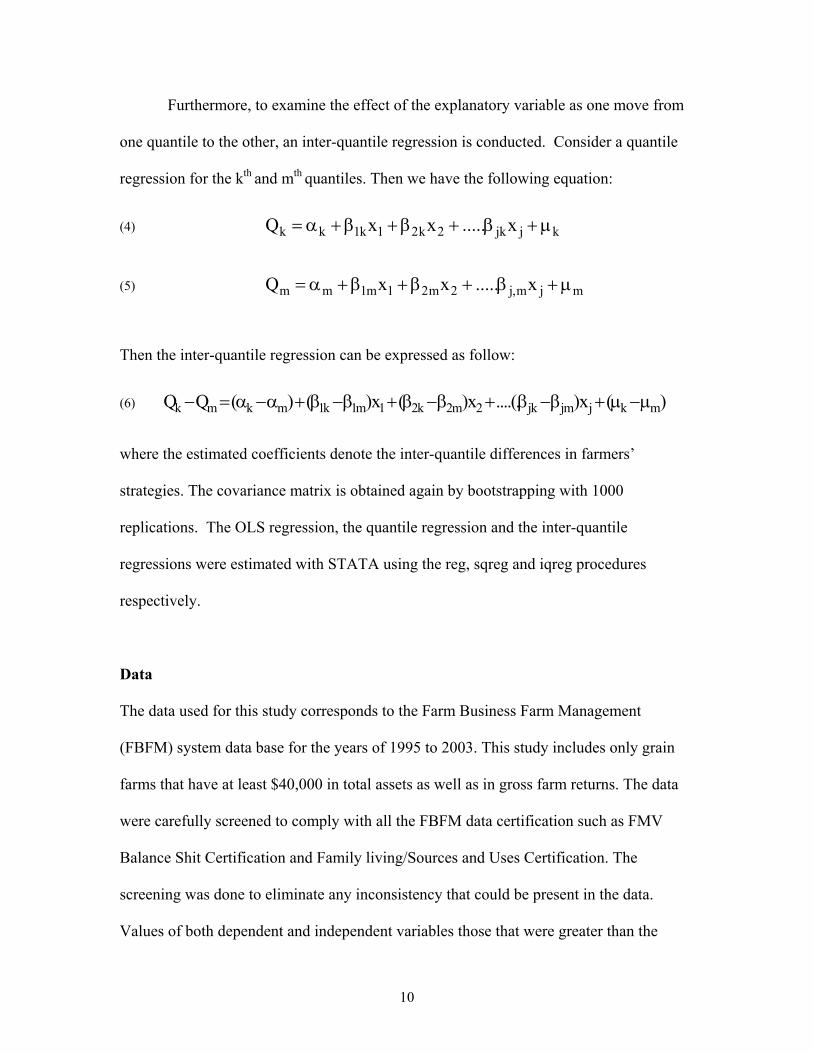
Furthermore, to examine the effect of the explanatory variable as one move from

one quantile to the other, an inter-quantile regression is conducted. Consider a quantile

regression for the kth and mth quantiles. Then we have the following equation:

(4) k k 1k 1 2k 2 jk j kQ x x ..... x= α +β +β + β + µ

(5) m m 1m 1 2m 2 j,m j mQ x x ..... x= α +β +β + β + µ

Then the inter-quantile regression can be expressed as follow:

(6) k m k m 1k 1m 1 2k 2m 2 jk jm j k mQ Q ( ) ( )x ( )x ....(. )x ( )− = α −α + β −β + β −β + β −β + µ −µ

where the estimated coefficients denote the inter-quantile differences in farmers’

strategies. The covariance matrix is obtained again by bootstrapping with 1000

replications. The OLS regression, the quantile regression and the inter-quantile

regressions were estimated with STATA using the reg, sqreg and iqreg procedures

respectively.

Data

The data used for this study corresponds to the Farm Business Farm Management

(FBFM) system data base for the years of 1995 to 2003. This study includes only grain

farms that have at least $40,000 in total assets as well as in gross farm returns. The data

were carefully screened to comply with all the FBFM data certification such as FMV

Balance Shit Certification and Family living/Sources and Uses Certification. The

screening was done to eliminate any inconsistency that could be present in the data.

Values of both dependent and independent variables those that were greater than the

11

mean plus three standard deviations or lower than the mean minus three standard

deviations were considered outliers, and consequently were eliminated from the sample.

These elimination procedures resulted in a sample of 3,212 farm observations for the year

1995 to 2003.

Table 1 shows the descriptive statistics of the variables employed in this study by

quantile of equity growth. The number of observations for each quantile varies between

321 and 322. The distribution of the observations among all quantiles is uniform within

the range mentioned above, as expected. Farms that experience the largest equity growth

are logically in the 90th quantile and have a 16% of equity growth on average. On the

other hand, farms that belong to the 10th quantile have a negative equity growth of 14%.

The asset turnover, debt to asset ratio, and interest expenses variables present a

U-shape relationship with the equity growth rate, as shown in Figure 1. The highest and

lowest quantiles are associated with the highest values of the ratios mentioned above.

For example, the mean for the asset turnover ratio is 37% for the 10th quantile and 34%

for the 90th quantile; middle quantiles such as 50th and 60th quantiles have on average an

asset turnover ratio of 27% and 28% respectively. This figure shows evidence that the

relationship between independent variables and equity growth may not be linear. The

same type of association is observed for the leverage variable. Similar to Escalante and

Barry (2002) findings, higher leverage ratios are observed for the highest and lowest

quantiles suggesting a dual nature of the leverage effect on equity growth.

Conversely, the tenure ratio presents an inverted U shape relationship with equity

growth; the higher and lower quantiles of farm equity growth are associated with lower

12

tenure ratio while middle quantiles show higher levels of the same ratios. The means of

tenure ratio for the 10th, 60th and 90th quantiles are 15%, 20% and 15% respectively.

The other variables used in this study do not have a single type of relationship

with the rate of equity growth. It is interesting to note that the family living expenses

variable as well as the operating expenses ratio decreases as moving up on the growth

quantile; higher equity growth rates are associated with low levels of family and

operating expenses. The mean value of family living expenditure for the 10th quantile is

$48,519 and for the 90th quantile is $48,022 whereas the mean of operating expenses ratio

for the 10th quantile is 71% and for the 90th quantile is 59%. The share leasing, the net

farm income and the off farm income ratios show a different behavior than the previous

group; the higher quantiles are related with the higher value of these ratios as expected.

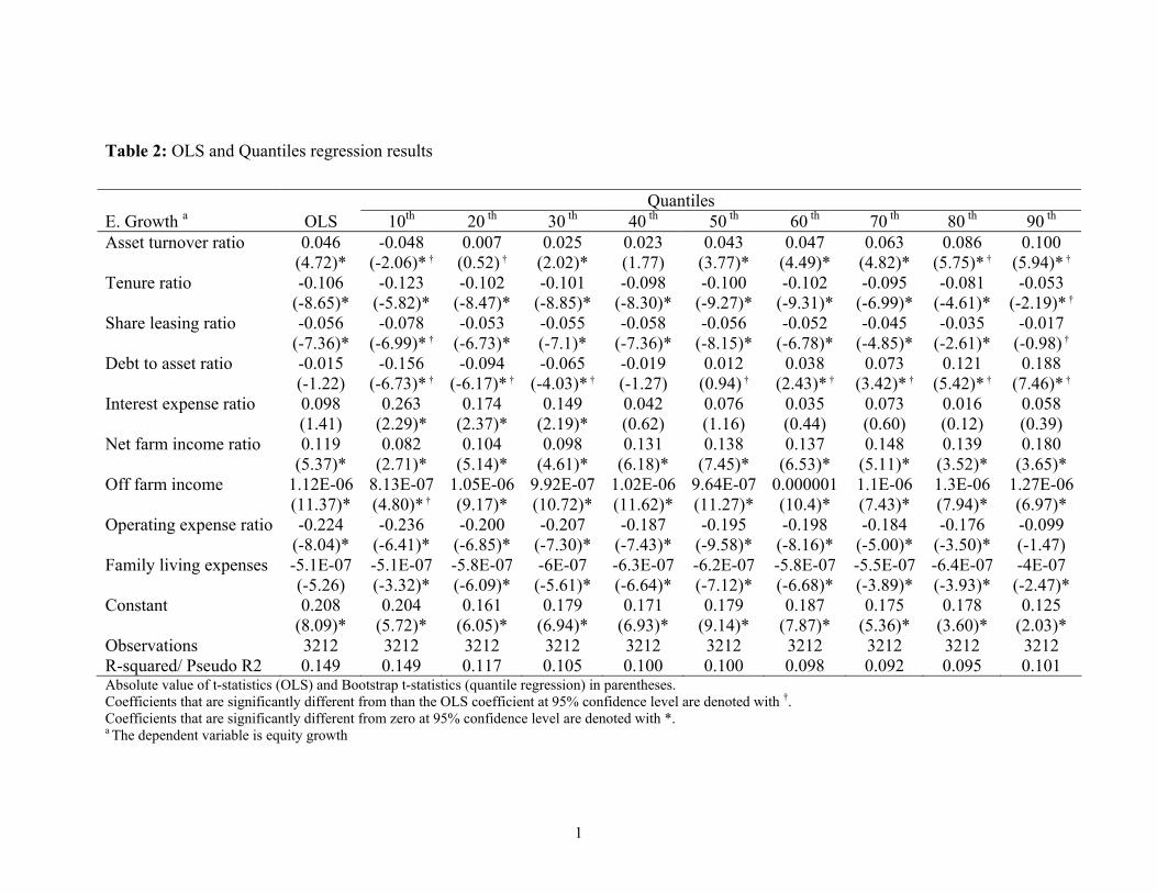
Regression Results

The results of the OLS regression as well as the results from the quantile regression are

shown in Table 2. Estimated coefficients for the asset turnover ratio, net farm income

ratio and off-farm income show a positive and significant impact of these variables on

equity growth ratio while tenure, share leasing ratio, operating expenses ratio and family

expenses have significantly negative effects on equity growth. The debt to asset and

interest expense ratios estimated coefficients are not significant. However, a Breusch-

Pagan test for heteroskedasticity indicates that heteroskedasticity is present in the data.1

The conditional variance of the equity growth distribution is not constant across different

levels of equity growth ratios. The presence of heteroskedasticity violates one of the

1 To test for heteroskedasticity, the hettest command on STATA was employed. The hettest performs a score (Lagrange multiplier) test for H: b=0 against multiplicative heteroskedasticity (Breusch & Pagan 1979; Cook & Weisberg 1983)

13

main assumptions of OLS: spherical errors. This leads to OLS estimates being inefficient.

Furthermore, quantile regression has the advantage that it does not assume normally

distributed errors for the estimation of the coefficients, as OLS does and allows

coefficients to change for different sub-sets of the sample. Pooling together all the data

may obscure interesting patterns in the behavior of farms with different equity growth

ratios. Quantile estimates improve the efficiency of the estimators compared to OLS and

allow analyzing independently heterogeneous farms. They may allow detecting

significant effects from variables whose coefficients may have been dismissed for not

appearing to be statistically different from zero in a mean based model such as OLS.

The low R2 of the OLS could be interpreted as evidence of bias due to omitted

variables; quantile method is also a good alternative when this type of bias is suspected

(Jayachandram, 2002). Nevertheless, the pseudo R2 which is the relevant goodness of fit

measure in quantile regression does not seem to show an improvement on the fit of the

model compared to OLS. Furthermore, the model appears to explain better the equity

growth for the lower two quantiles than for higher quantiles.

Table 2 shows that there exists a disparity in the behavior of farms which would

not be observed if we had looked only at the results from the OLS regression.

Specifically, two interesting cases are observed in the sign changes of the coefficients of

asset turnover ratio and debt to asset ratio. The asset turnover ratio has a positive impact

on equity growth for all quantiles except for the lowest one. As the percentile increase,

the magnitude of the coefficients also increases. This indicates that the effect of the asset

turnover ratio is more important for farms that have higher equity growth than for those

with low equity growth. Similarly for the lowest and highest quantiles, the estimated

14

coefficients are significantly different from the OLS coefficients. This can be seen on

Figure 2a where the 95% confidence interval for the quantile regression estimates for the

10th and 20th quartiles are below the OLS estimate. On the other hand, the confidence

interval for the quantile estimators for the 80th and 90th quantiles, is above the OLS

estimate. This result indicates that high equity growth farms make better use of its assets

to generate revenues than low equity growth farms.

The tenure ratio affects negatively the rate of equity growth for all quantiles

contrary to what was expected. These coefficients are significantly different from zero at

95% confidence. However only the 90th percentile estimated coefficient is significantly

different from the OLS estimator. Figure 2b shows that the OLS estimator for the tenure

ratio rest within the 95% confidence interval at each quantile except for the last one.

The share leasing ratio also has a negative effect on equity growth and is

significantly different from zero for all quantiles except for the 90th one. The 10th and

90th quantile coefficients are significantly different from the OLS coefficient as well.

These results indicate that greater reliance on owned and shared leased acres affect

negatively the rate of equity growth. This contradicts results from previous studies where

share leasing rate and tenure ratio showed a positive effect on equity. This change in sign

might be explained by the fact that cash rent arraignment appears to dominate the leasing

arraignment.

It is very interesting to observe that the leverage ratio is significantly different

from zero for all quantiles except for the middle one. The impact of leverage is negative

for farms that are in lower quantiles; however, for farms in the higher quantiles the effect

is reversed. Figure 2d shows this relationship as well as the fact that all quantile estimates

15

are significantly different from the OLS estimators. These results suggest that a higher

leverage position is an important determinant for those farms that already have a high rate

of equity growth. For farms in the opposite extreme of the distribution, high levels of

leverage have negative effects on equity growth; high leverage positions can be

associated with financially stressed farms that are not able to generate enough returns to

surpass the cost of borrowing resulting in a further deterioration in the farm equity

position. Financial strategies used by farms have different effects for each level of equity

growth. The interest expense ratio, on the other hand, is positive and significant only for

the low quantiles with the magnitude of the effect decreasing as the percentiles increases.

This indicates that the interest expense ratio is not detrimental for slow growing farms.

The revenue enhancement strategies represented by net farm income ratio and by

off farm income positively affect the equity growth of the farm. The net farm income

ratio as well as off-farm income coefficient estimates are significantly different from zero

for all quantiles. Nevertheless, whereas for net farm income none of the coefficients

estimated are statistically different from the OLS estimates, for the case of off-farm

income, Table 2 shows that the 10th quantile coefficient is in fact statistically different

from OLS. Figure 1f confirms the result expressed in Table 2 as it shows that OLS

estimates for this variable’s lie within the 95% confidence interval for quantile estimates.

Similarly Figure 1g shows that the OLS coefficient is outside the confidence interval only

for the 10th quantile as expressed above. These results indicate that even though the

revenue enhancement strategies are important determinants of net farm worth, in general

they are not affected by the position of the farm on the equity growth distribution.

16

The OLS estimator on the operating expense ratio variable confirms its expected

negative effect on equity growth. The coefficients on this variable are generally higher in

absolute value for higher quantiles than for the lower ones, suggesting that this variable

becomes more important for slower growing farms. In other words, the operating expense

ratio seems to be more of a negative factor for slower growing farm. Even though the

coefficients for all quantiles but the highest one are statistically different from zero they

are not statistically different from the OLS estimator.

The family living expenditure withdrawals negatively affect the equity growth of

farms. As it occurred for the operating expense ratio coefficients for all quantiles are

statistically different from zero but not from the OLS estimator. The highest effect in

absolute value is seen for the 40th percentile.

The results reported in Table 2 suggest that the magnitude of the coefficients

differ among quantiles for some of the variables included in the regressions. Inter-

quantile regressions are used to test this more rigorously by comparing the coefficients

across quantiles and determining whether or not they are statistically different from each

other. In particular, if the estimator of the interquantile regression for a certain variable is

significant then one can conclude that the slope parameters from the quantile regression

of such variable for the quantiles being compared are statistically different from each

other. Inter-quantile regression is a good way of further inspecting how farmers’

strategies change as one moves along the return on equity distribution. This allows to test

whether the effect of different business strategies is the same at two different quantiles.

Table 3 presents the results from the inter-quantile regressions, comparing only

contiguous quantiles. The effects of the asset turnover ratio appear to be different

17

between the 10th and the 20th quantile, the 40th and the 50th, and the 70th and the 80th. The

estimates of the coefficients of tenure ratio, off-farm income, operating expense ratio, and

family living expenditure does not appear to be statistically different across quintiles. For

the leverage ratio, it is clear that the effect is different for adjacent quantiles confirming

the conclusions expressed above. The larger differences are observed between the lowest

and highest interquantile ranges.

The interest expense ratio and net farm income effect appears to be different only

between the 30th to 40th quantile, while the share leasing ratio shows a difference only

between the 10th and 20th quantiles.

18

Summary and Conclusions

The empirical analysis takes into account the heterogeneity of the farm equity growth

using the quantile regressions approach, showing that OLS estimation is not always an

appropriate method to analyze equity growth. All the independent variables have been

found to have an influence on the net worth of the farm. However the importance of each

one of the strategies is not the same for all farms. All four strategies complement each

other to allow farms to maintain equity growth and to avoid its deterioration. The study

found that asset management strategies are an important determinant of the equity growth

for all farms; financial management strategies are relevant as well. Minimizing borrowing

costs or regulating the interest expenses through refinancing strategies and on time loan

payment, influence equity growth; however it is important to recognize that the effect of

these strategies depends on the location of the farm on the equity growth distribution.

This is the case in particular of the Financial Management strategy, measured through the

debt to asset ratio. Financially stressed farms use financial strategies differently than

farms that are well performed. Furthermore, the cost reduction strategies are also

important determinants of farm net worth. The regulation of family living withdrawals

and use of cost efficient technologies prevent the potential deterioration of farm equity.

By employing quantile a regression method, the findings of our study provide important

insights on the way farms use different business strategies to enhance farm net worth,

controlling for the unrealized nominal capital gains on farmland.

19

References

Barry, P., C. Escalante,a and S. Bard. “Economic Risk and the Structural Characteristics

of Farm Businesses.” Agricultural Finance Review, 61 (2001):73-86.

Boessen, C.R., A.M. Featherstone, L.N Langemeier, and R.O Burton, Jr. “Financial

Successful and Unsuccessful Farms.” J. Amer. Soc. of farm Managers and Rural

Appraisers 54(1990):6-15.

Buchinsky, S.A, M. Lino, S.A Gerrior, and P.P Basiotis. The healthy eating Index: 1994-

1996. Washington DC: U.S. Department of Agriculture, Center for Nutrition

Policy and Promotion, CNPP-5, July 1998.

______“Recent advances in Quantile Regression Models: A Practical Guideline for

Empirical Research.” J. Human Resources. 33 (1998):88-126.

Escalante, C.L, and P.J. Barry. “Risk Balancing in Integrated Farm Risk Management

Plan.” Journal of Agricultural and Applied Economics 33(2001):413-29.

Gorg H., E. Strobl, and F. Ruane. “Determinant of Firm Star-Up Size: An application of

Quantile Regression for Ireland.” Small Business Economics 14 (2000):211-222.

Jayachandram N., J, Blaylock, and D. Smallwood. “Characterizing the Distribution of

Macronutrients Intake among U.S. Adults: A Quantile Regression Approach”

Amer. J. Agr. Econ 84(2) (2002): 454-466.

Johnson,P., C. Conway, and P. Kattuman. “Small Business Growth in the Short Run.”

Small Business Economics 12(1999):103-12

Koenker, R. and G. Bassett. “Regression Quantiles.” Econometrica 46 (1978):33-50.

20

Purdy, B. M., M. R. Langemeier, and A. M. Featherstone. “Financial Performance, Risk,

and Specialization.” Journal of Agricultural and Applied Economics

29(1997):149-161.

Roper, S. “Modeling Small Business Growth and Profitability” Small Business

Economics 13(3):235 – 252.

U. S Department of Agriculture/Economics Research Service (USDA.ERS)

http://www.ers.usda.gov/

Voulgaris, F., D. Asteriou, and G. Agiomirgianakis. “The Determinants of Small Firm

Growth in the Greek Manufacturing Sector” Journal of Economic Integration

4(2003):817-36 .

1

Table 1: Descriptive Statistics by Quantiles

Quantiles Variables Mean 10 th 20 th 30 th 40 th 50 th 60 th 70 th 80 th 90 th Equity growth 0.05 -0.14 -0.04 -0.01 0.01 0.03 0.05 0.08 0.11 0.16 Asset turnover ratio 0.31 0.37 0.28 0.25 0.27 0.27 0.28 0.30 0.31 0.34 Tenure ratio 0.18 0.15 0.21 0.26 0.24 0.20 0.19 0.16 0.16 0.15 Share leasing ratio 0.55 0.54 0.55 0.50 0.52 0.56 0.55 0.57 0.57 0.58 Debt to asset ratio 0.31 0.45 0.31 0.26 0.28 0.27 0.26 0.28 0.30 0.32 Interest expense ratio 0.02 0.03 0.03 0.02 0.02 0.03 0.02 0.02 0.02 0.02 Net farm income ratio 0.20 0.09 0.15 0.18 0.19 0.22 0.22 0.23 0.24 0.24 Off farm income 20582 16228 17528 18790 21807 20457 21259 22670 21938 22301 Operating expense ratio 0.63 0.71 0.67 0.65 0.64 0.61 0.62 0.61 0.59 0.59 Family living expenses 48519 50546 49471 49427 48507 49056 46892 46399 48004 48022 Observations 321 322 321 321 322 321 321 322 321 321

1

Table 2: OLS and Quantiles regression results

Quantiles E. Growth a OLS 10th 20 th 30 th 40 th 50 th 60 th 70 th 80 th 90 th

0.046 -0.048 0.007 0.025 0.023 0.043 0.047 0.063 0.086 0.100 Asset turnover ratio (4.72)* (-2.06)* † (0.52) † (2.02)* (1.77) (3.77)* (4.49)* (4.82)* (5.75)* † (5.94)* †

-0.106 -0.123 -0.102 -0.101 -0.098 -0.100 -0.102 -0.095 -0.081 -0.053 Tenure ratio (-8.65)* (-5.82)* (-8.47)* (-8.85)* (-8.30)* (-9.27)* (-9.31)* (-6.99)* (-4.61)* (-2.19)* †

-0.056 -0.078 -0.053 -0.055 -0.058 -0.056 -0.052 -0.045 -0.035 -0.017 Share leasing ratio (-7.36)* (-6.99)* † (-6.73)* (-7.1)* (-7.36)* (-8.15)* (-6.78)* (-4.85)* (-2.61)* (-0.98) †

-0.015 -0.156 -0.094 -0.065 -0.019 0.012 0.038 0.073 0.121 0.188 Debt to asset ratio (-1.22) (-6.73)* † (-6.17)* † (-4.03)* † (-1.27) (0.94) † (2.43)* † (3.42)* † (5.42)* † (7.46)* †

0.098 0.263 0.174 0.149 0.042 0.076 0.035 0.073 0.016 0.058 Interest expense ratio (1.41) (2.29)* (2.37)* (2.19)* (0.62) (1.16) (0.44) (0.60) (0.12) (0.39)

0.119 0.082 0.104 0.098 0.131 0.138 0.137 0.148 0.139 0.180 Net farm income ratio (5.37)* (2.71)* (5.14)* (4.61)* (6.18)* (7.45)* (6.53)* (5.11)* (3.52)* (3.65)*

1.12E-06 8.13E-07 1.05E-06 9.92E-07 1.02E-06 9.64E-07 0.000001 1.1E-06 1.3E-06 1.27E-06Off farm income (11.37)* (4.80)* † (9.17)* (10.72)* (11.62)* (11.27)* (10.4)* (7.43)* (7.94)* (6.97)*

-0.224 -0.236 -0.200 -0.207 -0.187 -0.195 -0.198 -0.184 -0.176 -0.099 Operating expense ratio (-8.04)* (-6.41)* (-6.85)* (-7.30)* (-7.43)* (-9.58)* (-8.16)* (-5.00)* (-3.50)* (-1.47)

-5.1E-07 -5.1E-07 -5.8E-07 -6E-07 -6.3E-07 -6.2E-07 -5.8E-07 -5.5E-07 -6.4E-07 -4E-07 Family living expenses (-5.26) (-3.32)* (-6.09)* (-5.61)* (-6.64)* (-7.12)* (-6.68)* (-3.89)* (-3.93)* (-2.47)*

0.208 0.204 0.161 0.179 0.171 0.179 0.187 0.175 0.178 0.125 Constant (8.09)* (5.72)* (6.05)* (6.94)* (6.93)* (9.14)* (7.87)* (5.36)* (3.60)* (2.03)* Observations 3212 3212 3212 3212 3212 3212 3212 3212 3212 3212 R-squared/ Pseudo R2 0.149 0.149 0.117 0.105 0.100 0.100 0.098 0.092 0.095 0.101 Absolute value of t-statistics (OLS) and Bootstrap t-statistics (quantile regression) in parentheses. Coefficients that are significantly different from than the OLS coefficient at 95% confidence level are denoted with †. Coefficients that are significantly different from zero at 95% confidence level are denoted with *. a The dependent variable is equity growth

1

Table 3: Inter-Quantile regression results

Inter-Quantiles

10th –20th 20th –30th 30th –40th 40th –50th 50th –60th 60th –70th 70th –80th 80th – 90th Asset turnover ratio 0.055 0.018 -0.003 0.021 0.004 0.016 0.023 0.014 (3.26)* (1.83) (-0.32) (2.67)* (0.55) (1.80 (2.16)* (1.01) Tenure ratio 0.021 0.001 0.003 -0.002 -0.002 0.007 0.014 0.028 (1.38) (0.10) (0.32) (-0.3) (-0.26) (0.83) (1.07) (1.45) Share leasing ratio 0.025 -0.003 -0.002 0.002 0.004 0.007 0.010 0.018 (2.94)* (-0.46) (-0.48) (0.35) (0.87) (1.07) (1.02) (1.32) Debt to asset ratio 0.061 0.029 0.047 0.031 0.025 0.036 0.047 0.067 (3.29)* (2.72)* (4.50)* (3.55)* (2.84)* (2.71)* (3.00)* (3.18)* Interest expense ratio -0.089 -0.026 -0.106 0.033 -0.040 0.038 -0.058 0.042 (-0.97) (-0.51) (-2.20)* (0.76) (-0.79) (0.51) (-0.67) (0.33) Net farm income ratio 0.022 -0.006 0.033 0.007 -0.001 0.011 -0.009 0.041 (0.99) (-0.37) (2.34)* (0.49) (-0.1) (0.60) (-0.30) (1.11) Off farm income 2.38E-07 -5.9E-08 2.77E-08 -5.5E-08 3.75E-08 9.52E-08 2.05E-07 -3.1E-08 (1.70) (-0.81) (0.44) (-0.95) (0.58) (0.99) (1.81) (-0.20) Operating expense ratio 0.036 -0.007 0.020 -0.008 -0.003 0.014 0.008 0.076 (1.26) (-0.35) (1.18) (-0.48) (-0.18) (0.59) (0.22) (1.58) Family living expenditure -6.9E-08 -2.3E-08 -3E-08 1.22E-08 4.11E-08 3.24E-08 -9.1E-08 2.33E-07 (-0.55) (-0.30) (-0.44) (0.2) (0.67) (0.36) (-0.79) (1.65) Constant -0.042 0.017 -0.007 0.008 0.008 -0.012 0.003 -0.053 (-1.60) (0.92) (-0.46) (0.51) (0.51) (-0.55) (0.09) (-1.22) Observations 3212 3212 3212 3212 3212 3212 3212 3212 Pseudo R2 0.149 0.1172 0.1046 0.0996 0.0996 0.0977 0.092 0.1007 Bootstrap t-statistics values in parentheses. Coefficients that are significantly different from zero at 95% confidence level are denoted with *

1

Figure 1: Mean values of Selected Variables by Quantiles of Equity Growth

Asset Turnover Ratio

0.000.100.200.300.40

10 20 30 40 50 60 70 80 90

Quantiles

Perc

ent

T enure Ratio

0.00

0.10

0.20

0.30

10 20 30 40 50 60 70 80 90

Quantiles

Perc

ent

Share Leasing Ratio

0.45

0.50

0.55

0.60

10 20 30 40 50 60 70 80 90

Quantiles

Perc

ent

Debt-to-Asset Ratio

0.00

0.20

0.40

0.60

10 20 30 40 50 60 70 80 90

Quantiles

Perc

ent

Interest Expense Ratio

0.000.010.020.030.04

10 20 30 40 50 60 70 80 90

Quantiles

Perc

ent

Net Farm Income Ratio

0.00

0.10

0.20

0.30

10 20 30 40 50 60 70 80 90

Quantiles

Perc

ent

2

Off Farm Income

0

10000

20000

30000

10 20 30 40 50 60 70 80 90

Quantiles

Dol

ars

Operating Expense Ratio

0.550.600.650.700.75

10 20 30 40 50 60 70 80 90

Quantiles

Perc

ent

Famliy Living Expenses

46000

48000

50000

52000

10 20 30 40 50 60 70 80 90

Quantiles

Dol

ars

Equity Growth

-0.20-0.100.000.100.20

10 20 30 40 50 60 70 80 90

Quantiles

Perc

ent

3

Figure 2: Quantile Regression Results

Asset T urnover Rat io Coefficients

-0.15

-0 .10

-0.05

0.00

0.05

0.10

0.15

10 20 30 40 50 60 70 80 90Quant iles

OLS C o efficient Quant ile C o efficientLo wer B o und Up p er B o und

T urnover Rat io Coefficients

-0 .18-0.16-0.14-0.12-0.10-0.08-0.06-0.04-0.020.00

10 20 30 40 50 60 70 80 90

Quant ilesOLS C o efficient Quant ile C o efficientLo wer B o und Up p er B o und

Share Leasing Rat io Coefficients

-0 .12-0 .10-0 .08-0 .06-0 .04-0 .020.000.020.04

10 20 30 40 50 60 70 80 90Quant iles

OLS C o efficient Quant ile C o efficientLo wer B o und Up p er B o und

Debt -to-Asset Rat io Coefficients

-0 .30

-0 .20

-0 .10

0.00

0.10

0.20

0.30

10 20 30 40 50 60 70 80 90Quant iles

OLS C o efficient Quant ile C o efficientLo wer B o und Up p er B o und

Interest Expense Rat io Coefficients

-0.40

-0.20

0.000.20

0.40

0.60

10 20 30 40 50 60 70 80 90Quant iles

OLS C o efficient Quant ile Co efficientLo wer B o und Up p er B o und

Net Farm Income Rat io Coefficient s

0.00

0.10

0.20

0.30

10 20 30 40 50 60 70 80 90Quant iles

OLS C o efficient Quant ile C o efficientLo wer B o und Up p er B o und

4

Off-Farm Income Coefficients

0.0E+00

5.0E-07

1.0E-06

1.5E-06

2.0E-06

10 20 30 40 50 60 70 80 90Quant iles

OLS Coefficient Quant ile CoefficientLo wer Bo und Up per Bound

Operating Expenses Ratio Coefficients

-0.40-0.30-0.20-0.100.000.10

10 20 30 40 50 60 70 80 90Quant iles

OLS Coefficient Quantile CoefficientLo wer Bo und Upp er Bound

Family Living Expenses Coefficients

-1.2E-06

-1.0E-06

-8.0E-07

-6.0E-07

-4.0E-07

-2.0E-07

0.0E+00

10 20 30 40 50 60 70 80 90

QuantilesOLS Coefficient Quant ile CoefficientLo wer Bo und Up per Bound