Fibonacci arithmetic expressions

Automation and Remote Control, Vol. 65, No. 6, 2004, pp. 842–856. Translated from Avtomatika i Telemekhanika, No. 6, 2004, pp. 4–21.Original Russian Text Copyright c© 2004 by Astola, Egiazarian, M. Stankovic, R. Stankovic.

ARITHMETIC LOGIC

Fibonacci Arithmetic Expressions1

J. T. Astola∗, K. Egiazarian∗, M. Stankovic∗∗, and R. S. Stankovic∗∗

∗Tampere International Center for Signal Processing, Tampere University of Technology, Tampere, Finland∗∗University of Nis, Dept. of Computer Science, Faculty of Electronics, Nis, Serbia

Received December 16, 2003

Abstract—In this paper, we extend the arithmetic (AR) expressions for functions on finitedyadic groups to functions used in Fibonacci interconnection topologies. We have introduced theFibonacci-Arithmetic (FibAR) expressions for representation of these functions. We discussedthe optimization of FibARs with respect to the number of non-zero coefficients through theFixed-Polarity FibARs defined by using different polarities for the Fibonacci variables. In thisway, we provide a base to extend the application of ARs and related powerful CAD design toolsfor switching functions to functions in Fibonacci interconnection topologies.

1. INTRODUCTION

Arithmetic expressions (ARs) for switching functions were used in the description of logic net-works from the beginning of development of this area [1–4], see also [5, 6]. Although ARs forswitching functions, are hybrid expressions in the sense that the coefficients are integers for thelogic-valued functions, there is apparent a renewed interest in application of ARs for the followingreasons:

(1) ARs are useful in parallelization of algorithms for calculations with switching functions[5, 7, 8],

(2) ARs can represent the multi-output switching functions by a single expression which cannotbe done with bit-level expressions [9, 10,12],

(3) ARs belong to the class of word-level expressions for switching functions in form of whichsome word-level decision diagrams represent the switching functions [13–15],

(4) ARs can be used to estimate the error probability in logic networks [5].Boolean interconnection topologies are extensively used in systems design, and logic design, see

for example [6,21]. However, in some applications, they express some inconveniences originating intheir inherent features, as for example, restrictions to the power of two in the number of nodes orinputs, etc. For this reason, the Fibonacci interconnection topologies are offered as an alternative[22–26].

With this motivation, in this paper we extended the ARs to functions defined in a number ofpoints equal to a generalized Fibonacci p-number.

2. NOTATIONS

The Boolean interconnection topologies are used in the design of systems whose input and outputsignals are described by functions defined in 2n points, where n ∈ N0 = N ∪ 0, N is the set ofnatural numbers. Each point is represented by an n-tuple x = (x1, . . . , xn), xi ∈ {0, 1}, determined

as the binary representation for x, i.e., x =n∑

i=12ixi. We denote the set of such n-tuples by Cn

2 and

1 This work was supported by the Academy of Finland, project no. 44876 and EXSITE, project no. 51520.

0005-1179/04/6506-0842 c© 2004 MAIK “Nauka/Interperiodica”

FIBONACCI ARITHMETIC EXPRESSIONS 843

Table 1. Binary representations of integers Table 2. Fibonacci 1-code representations of integers

i c1c2c3 x1x2x3

0 000 x1x2x3

1 001 x1x2x3

2 010 x1x2x3

3 011 x1x2x3

4 100 x1x2x3

5 101 x1x2x3

6 110 x1x2x3

7 111 x1x2x3

i d1d2d3d4 w1w2w3w4

0 0000 w1w2w3w4

1 0001 w1w2w3w4

2 0010 w1w2w3

3 0100 w1w2w4

4 0101 w1w2w4

5 1000 w1w3w4

6 1001 w1w3w4

7 1010 w1w3

by P (Cn2 ) the space of functions f : Cn

2 → P , where P is a field that may be the complex field Cor a finite (Galois) field. The space of n-variable switching functions is a particular case whereP = GF (2).

In Fibonacci interconnection topologies, the input and output signals of systems are representedby functions defined in φp(i) points, where φp(i) is a generalized Fibonacci p-number [22,27]. Eachpoint is represented by a binary sequence w = (w1, . . . , wi−1)p in the Fibonacci p-code for w.We denote by Fn

2,p the set of such sequences, and by P (Fn2,p) the space of functions f : Fn

2,p → P .It should be noted that for p = 0, P (Fn

2,p) becomes P (Cn2 ).

In this paper, the presentation is illustrated by examples that are developed for functions definedin the number of points equal to the generalized Fibonacci 1-number φ1(5) = 8. Binary-valued func-tions defined in φ1(5) points correspond to three variable switching functions. Thus, such examplespermit a direct comparison of representations for functions in Boolean and Fibonacci topologies.However, all the considerations are true generally for functions defined in φp(i) points, wherep and i are arbitrary numbers permitted in the generalized Fibonacci p-numbers and codes [26].

Basic definitions and notations for the generalized Fibonacci numbers and codes are given inthe Appendix.

Example 1. Table 1 shows the representation of first eight non-zero integers by the natural

binary code defined as x =n∑

i=1xi2i. Table 2 shows the corresponding Fibonacci 1-code.

3. ARITHMETIC EXPRESSIONS

ARs for functions ∈ C(Cn2 ) can be introduced in the following way.

In Boolean expressions, we interpret the logic values 0 and 1 for the switching variables andfunction values as the integers 0 and 1, respectively, which we denote as the coding (0, 1)GF (2) →(0, 1)Z , and replace the Boolean operations by the corresponding arithmetic operations. Table 3shows the correspondence among these operations.

Table 3. Arithmetic operations for Boolean operations

Boolean Arithmetic

x 1− xx ∧ y xyx ∨ y x+ y − xyx ⊕ y x+ y − 2xy

AUTOMATION AND REMOTE CONTROL Vol. 65 No. 6 2004

844 ASTOLA et al.

Alternatively, we can consider the ARs as integer counterpart of Reed–Muller (RM) expressions,see for example, [12], and for a given f we determine the AR-expression for f by the recursive appli-cation of the arithmetic positive Davio (pDAR) expansion rule to all the variables in f . The pDAR-expansion rule is defined as f = 1 · f0 + xi(−f0 + f1), where f0 = f(x1, . . . , xi−1, 0, xi+1, . . . , xn)and f1 = f(x1, . . . , xi−1, 1, xi+1, . . . , xn).

From spectral interpretation of RMs, we determine the ARs as Fourier series-like expansionswith respect to the Reed–Muller functions defined by columns of the Reed–Muller matrices R(n) =n⊗

i=1R(1), where R(1) =

[1 01 1

]is the basic Reed–Muller matrix.

We define an integer counterpart of the RM-matrix as a matrix A(n) = R(n)(0,1)Zand determine

the coefficients in ARs by using a matrix A(n)−1 inverse to A(n) calculated over the field of rationalnumbers Q.

In symbolic notation, the RM-functions can be generated as X(n) =n⊗

i=1

[1 xi

], where ⊗

denotes the Kronecker product. We generate the integer RM function (iRM) in the same way,since they differ just in the interpretation of the values of switching variables.

Example 2. For n = 3, the columns of R(3) are the RM-functions described by product terms

X(3) =[1 x1

]⊗

[1 x2

]⊗

[1 x3

]= [1, x3, x2, x2x3, x1, x1x3, x1x2, x1x2x3] .

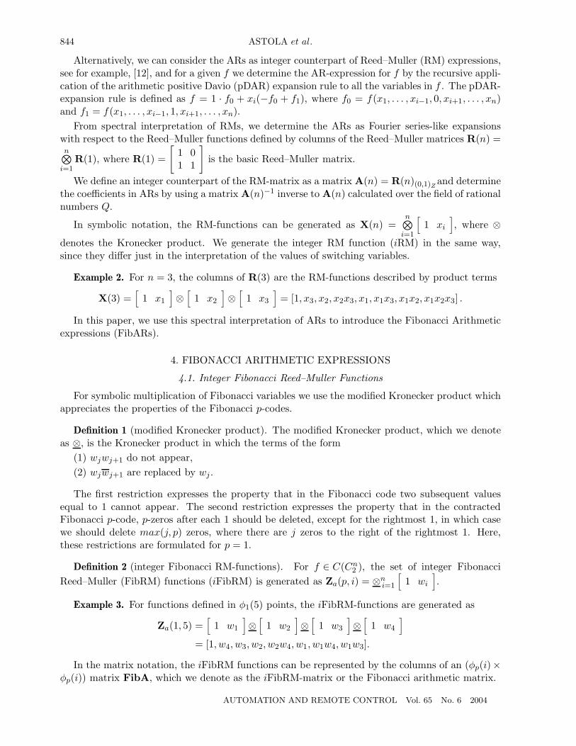
In this paper, we use this spectral interpretation of ARs to introduce the Fibonacci Arithmeticexpressions (FibARs).

4. FIBONACCI ARITHMETIC EXPRESSIONS

4.1. Integer Fibonacci Reed–Muller Functions

For symbolic multiplication of Fibonacci variables we use the modified Kronecker product whichappreciates the properties of the Fibonacci p-codes.

Definition 1 (modified Kronecker product). The modified Kronecker product, which we denoteas ⊗, is the Kronecker product in which the terms of the form

(1) wjwj+1 do not appear,(2) wjwj+1 are replaced by wj .

The first restriction expresses the property that in the Fibonacci code two subsequent valuesequal to 1 cannot appear. The second restriction expresses the property that in the contractedFibonacci p-code, p-zeros after each 1 should be deleted, except for the rightmost 1, in which casewe should delete max(j, p) zeros, where there are j zeros to the right of the rightmost 1. Here,these restrictions are formulated for p = 1.

Definition 2 (integer Fibonacci RM-functions). For f ∈ C(Cn2 ), the set of integer Fibonacci

Reed–Muller (FibRM) functions (iFibRM) is generated as Za(p, i) = ⊗ni=1

[1 wi

].

Example 3. For functions defined in φ1(5) points, the iFibRM-functions are generated as

Za(1, 5) =[1 w1

]⊗

[1 w2

]⊗

[1 w3

]⊗

[1 w4

]= [1, w4, w3, w2, w2w4, w1, w1w4, w1w3].

In the matrix notation, the iFibRM functions can be represented by the columns of an (φp(i)×φp(i)) matrix FibA, which we denote as the iFibRM-matrix or the Fibonacci arithmetic matrix.



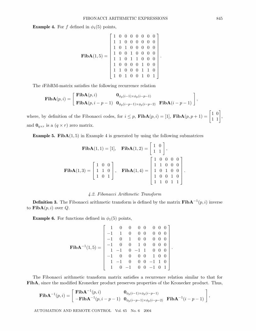
Example 4. For f defined in φ1(5) points,

FibA(1, 5) =

1 0 0 0 0 0 0 01 1 0 0 0 0 0 01 0 1 0 0 0 0 01 0 0 1 0 0 0 01 1 0 1 1 0 0 01 0 0 0 0 1 0 01 1 0 0 0 1 1 01 0 1 0 0 1 0 1

.

The iFibRM-matrix satisfies the following recurrence relation

FibA(p, i) =

[FibA(p, i) 0φp(i−1)×φp(i−p−1)

FibA(p, i − p − 1) 0φp(i−p−1)×φp(i−p−2) FibA(i − p − 1)

],

where, by definition of the Fibonacci codes, for i ≤ p, FibA(p, i) = [1], FibA(p, p + 1) =

[1 01 1

],

and 0q×r is a (q × r) zero matrix.

Example 5. FibA(1, 5) in Example 4 is generated by using the following submatrices

FibA(1, 1) = [1], FibA(1, 2) =

[1 01 1

],

FibA(1, 3) =

1 0 01 1 01 0 1

, FibA(1, 4) =

1 0 0 0 01 1 0 0 01 0 1 0 01 0 0 1 01 1 0 1 1

.

4.2. Fibonacci Arithmetic Transform

Definition 3. The Fibonacci arithmetic transform is defined by the matrix FibA−1(p, i) inverseto FibA(p, i) over Q.

Example 6. For functions defined in φ1(5) points,

FibA−1(1, 5) =

1 0 0 0 0 0 0 0−1 1 0 0 0 0 0 0−1 0 1 0 0 0 0 0−1 0 0 1 0 0 0 01 −1 0 −1 1 0 0 0

−1 0 0 0 0 1 0 01 −1 0 0 0 −1 1 01 0 −1 0 0 −1 0 1

.

The Fibonacci arithmetic transform matrix satisfies a recurrence relation similar to that forFibA, since the modified Kronecker product preserves properties of the Kronecker product. Thus,

FibA−1(p, i) =

[FibA−1(p, i) 0φp(i−1)×φp(i−p−1)

−FibA−1(p, i − p − 1) 0φp(i−p−1)×φp(i−p−2) FibA−1(i − p − 1)

],


846 ASTOLA et al.

Table 4. Expansion rules for Fibonacci PPARs

Expansion rule Transform matrices

f = 1 · f0 + wi(−f0 + f1) FibAR(1, 2) =[

1 0−1 1

]

f = 1 · f0 + wi+1(−f0 + f1) + wi(−f0 + f2) FibAR(1, 3) =

1 0 0

−1 1 0−1 0 1

where for i ≤ p, FibA−1(p, i) = [1], FibA−1(p, p + 1) =

[1 0

−1 1

], and 0q×r is a (q × r) zero

matrix.

Example 7. FibA−1(1, 5) in Example 6 is generated by using the following submatrices

FibA−1(1, 1) = [1], FibA−1(1, 2) =

[1 0

−1 1

],

FibA−1(1, 3) =

1 0 0−1 1 0−1 0 1

, FibA−1(1, 4) =

1 0 0 0 0−1 1 0 0 0−1 0 1 0 0−1 0 0 1 01 −1 0 −1 1

.

Definition 4. The Fibonacci arithmetic spectrum is defined as SFa,f = FibA−1(p, i)F.

4.3. Fibonacci Arithmetic Expressions

We define the Fibonacci arithmetic expressions (FibARs) as expressions for functions defined inφp(i) points whose coefficients are the Fibonacci arithmetic transform coefficients.

Definition 5. The positive-polarity Fibonacci arithmetic expression (FibPPAR) is defined asf = Za(p, i)FibA−1(p, i)F.

Example 8. For functions defined in φp(i) points, the FibPPAR-expression is defined as

f =([

1 w1

]⊗

[1 w2

]⊗

[1 w3

]⊗

[1 w4

])FibA−1(1, 5)F

= a0 ⊕ a1w4 ⊕ a2w3 ⊕ c3w2 ⊕ c4w2w4 ⊕ c5w1 ⊕ c6w1w4 ⊕ c7w1w3,

where ci are the Fibonacci PPAR-coefficients.

As is noted above, in Boolean topologies, the positive polarity RM-expressions are determined bythe recursive application of the positive Davio (pD) expansion f = 1 ·f0 ⊕xi(f0⊕f1). The positivepolarity ARs (PPARs) are determined by the recursive application of the pDAR-expansion derivedfrom pD expansion rule by the replacement of logic values 0 and with the integers 0 and 1, andEXOR with the addition in Q. The same can be done in the Fibonacci topologies. Table 4 showsthe Fibonacci arithmetic expansion rules derived for the basic FibAR-matrices for p = 1.

4.4. Fixed-polarity FibARs

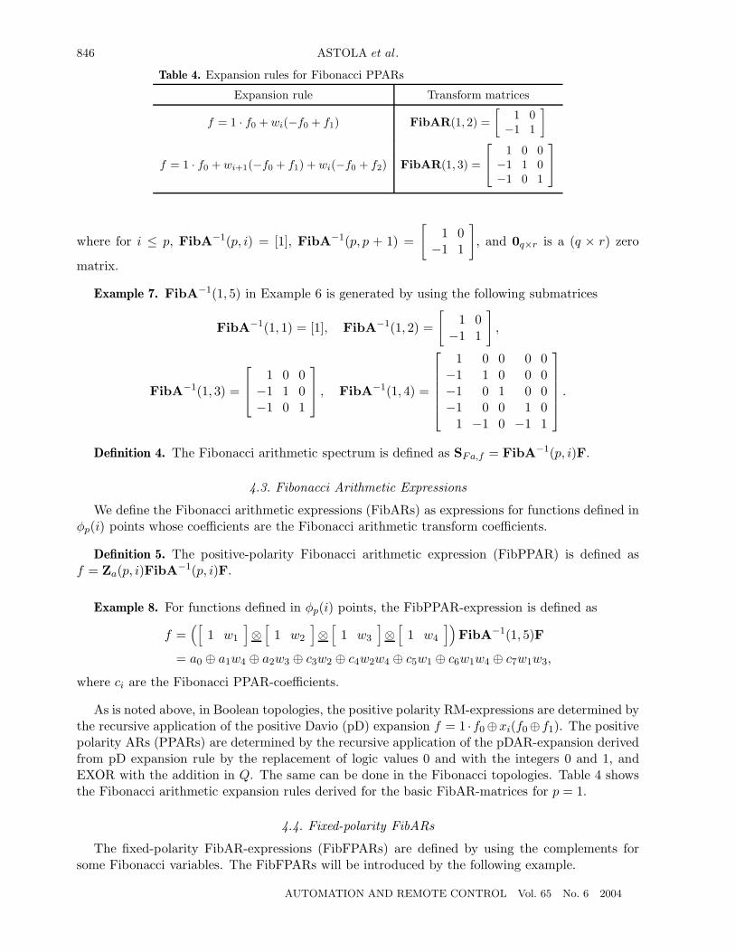
The fixed-polarity FibAR-expressions (FibFPARs) are defined by using the complements forsome Fibonacci variables. The FibFPARs will be introduced by the following example.



Table 5. Complements of Fibonacci variables

P1 P2 P3 P4 P 1 P 2 P 3 P 4

0 0 0 0 1 1 1 10 0 0 1 1 1 1 00 0 1 0 1 1 0 00 1 0 0 1 0 0 10 1 0 1 1 0 0 01 0 0 0 0 0 1 11 0 0 1 0 0 1 01 0 1 0 0 0 0 0

Example 9. For functions defined in φ1(5) points, if we use the positive literals for w1 and w3

and negative literals for w2 and w4, the FibA matrix for the polarity H = (0101) is given by

FibA(0101)(1, 5) =

1 1 0 1 1 0 0 01 0 0 1 0 0 0 01 0 1 1 0 0 0 01 1 0 0 0 0 0 01 0 0 0 0 0 0 01 1 0 0 0 1 1 01 0 0 0 0 1 0 01 0 1 0 0 1 0 1

.

Table 5 shows complements of Fibonacci variables for functions defined in φ1(p) points and usedin this matrix. Its columns can be described by products of Fibonacci variables appearing in theFibFPA for H = (0101). Thus, they are represented by

Z(0101)(1, 5) =[1 w1

]⊗

[1 w2

]⊗

[1 w3

]⊗

[1 w4

]= [1, w4, w3, w2, w2w4, w1, w1w4, w1w3].

It follows that the FibFPAR for H = (0101) is given by

f =([

1 w1

]⊗

[1 w2

]⊗

[1 w3

]⊗

[1 w4

])FibA−1

(0101)(1, 5)F= c0 ⊕ c1w4 ⊕ c2w3 ⊕ c3w2 ⊕ c4w2w4 ⊕ c5w1 ⊕ c6w1w4 ⊕ c7w1w3,

where ci are the Fibonacci FPAR-coefficients for H = (0101). They are calculated as followsSa,f,(0101) = FibA−1

(0101)(1, 5)F, where

FibA−1(0101)(1, 5) =

0 0 0 0 1 0 0 00 0 0 1 −1 0 0 00 −1 1 0 0 0 0 00 1 0 0 −1 0 0 01 −1 0 −1 1 0 0 00 0 0 0 −1 0 1 00 0 0 −1 1 1 −1 00 1 −1 0 0 0 −1 1

.

5. CALCULATION OF FIBONACCI ARITHMETIC COEFFICIENTS

The coefficients in FibARs can be calculated by using FFT-like algorithms derived in a waysimilar to that used in [26] to derive the corresponding algorithms for the Fibonacci Walsh andthe Fibonacci Haar transforms. For the inherent exponential complexity of FFT-like algorithms,


848 ASTOLA et al. f

0

f

1

f

0

–f

0

+

f

1

–1

–1

–1

f

2

f

3

f

4

f

5

f

6

f

7

f

7

–f

3

+

f

4

f

5

f

3

f

2

–1

–1

–f

5

+

f

6

f

0

–f

0

+

f

1

–f

5

+

f

7

–f

3

+

f

4

f

5

f

3

–f

0

+

f

2

–f

5

+

f

6

f

0

–f

0

+

f

1

–f

5

+

f

7

f

0

–

f

1

– f

3

+

f

4

f

5

–f

0

+

f

3

–f

0

+

f

2

–f

5

+

f

6

–1

–1

f

0

–f

0

+

f

1

f

0

–

f

2

– f

5

+

f

7

f

0

–

f

1

– f

3

+

f

4

–f

0

+

f

5

–f

0

+

f

3

–f

0

+

f

2

f

0

–

f

1

– f

5

+

f

6

–1

–1

–1

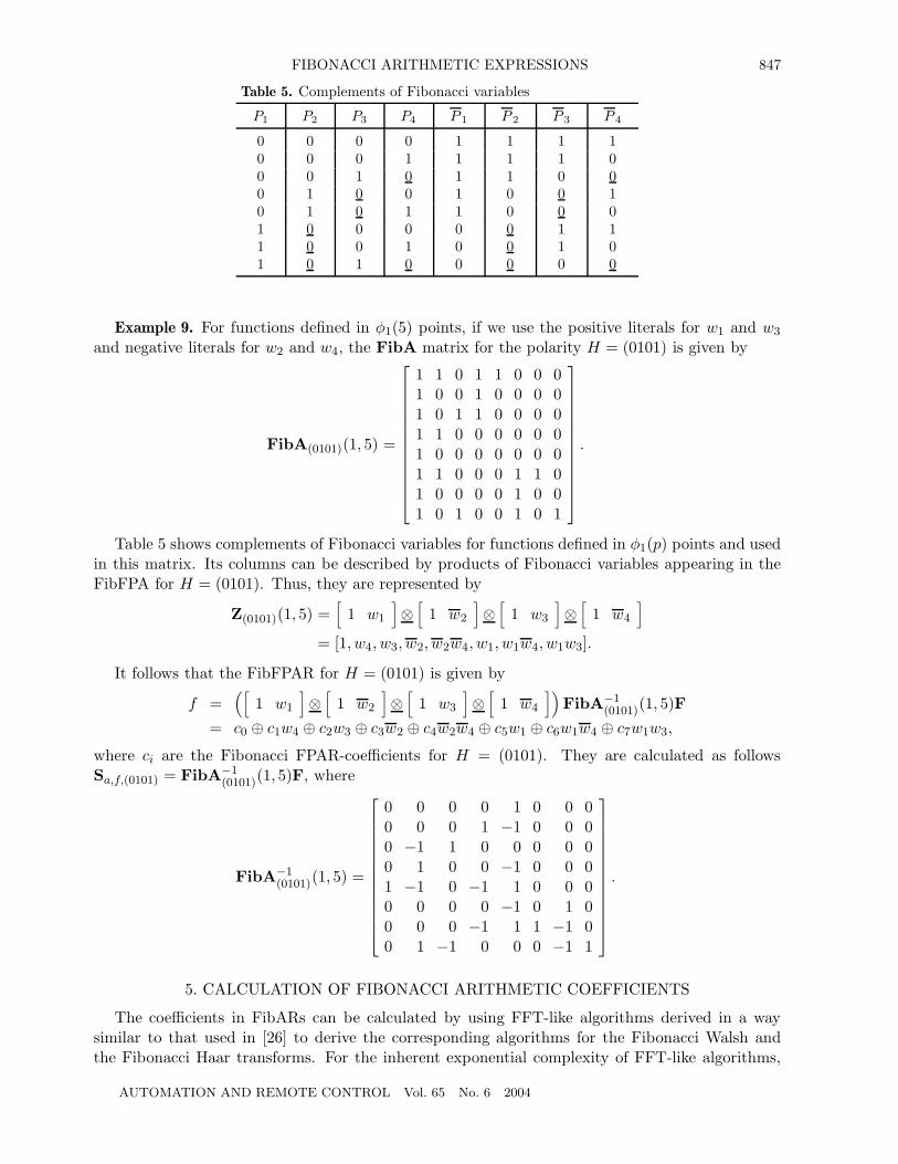
Fig. 1. FFT-like algorithm for FibARs for φ1(5).

we developed an algorithm for calculation of FibARs through the Fibonacci decision diagrams(FibDDs) in a way similar to that used in Boolean topologies to calculate the spectral transformsthrough the Binary decision diagrams (BDDs) [28,29], and Multi-terminal binary decision diagrams(MTBDDs) [30].

5.1. FFT-like Algorithms for FibARs

The FibARs preserve the properties of Fibonacci transforms, including the recurrence relationspermitting a factorization which enable derivation of FFT-like calculation algorithms [26]. In thecase of FibARs, these algorithms have a very simple structure, due to the wavelets like structureof the matrices FibA and FibA−1. FFT-like algorithms for calculation of coefficients in FibARswill be introduced by the following example.

Example 10. Figure 1 shows the flow-graph of the FFT algorithm for calculation of coefficientsin FibPPARs for functions defined in φ1(5) points.

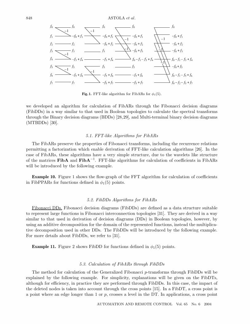
5.2. FibDDs Algorithms for FibARs

Fibonacci DDs. Fibonacci decision diagrams (FibDDs) are defined as a data structure suitableto represent large functions in Fibonacci interconnection topologies [31]. They are derived in a waysimilar to that used in derivation of decision diagrams (DDs) in Boolean topologies, however, byusing an additive decomposition for the domain of the represented functions, instead the multiplica-tive decomposition used in other DDs. The FibDDs will be introduced by the following example.For more details about FibDDs, we refer to [31].

Example 11. Figure 2 shows FibDD for functions defined in φ1(5) points.

5.3. Calculation of FibARs through FibDDs

The method for calculation of the Generalized Fibonacci p-transforms through FibDDs will beexplained by the following example. For simplicity, explanations will be given on the FibDTs,although for efficiency, in practice they are performed through FibDDs. In this case, the impact ofthe deleted nodes is taken into account through the cross points [15]. In a FibDT, a cross point isa point where an edge longer than 1 or p, crosses a level in the DT. In applications, a cross point



f

0

f

1

f

2

3

0 1

10

FB

FB

q

4,0

q

3,0

0

0

1

1

f

5

f

6

f

7

3

0 1

1

0

FB

FB

q

4,2

q

3,1

FB

0 1

f

3

f

4

2

q

4,1

FB

FB

q

1

q

2

x

Fig. 2. Fib1DT(5).

is considered as a node with both outgoing edges pointing to the same node at a subsequent levelin the DD.

Bottom-up strategy for FWHT. We assume that a function f defined in φp(i) points is givenby the truth-vector F = [f0, . . . , fφp(i)−1]T and represented by the FibpDT(i). We calculate theFibAR coefficients for f by using the following procedure.

Procedure for calculation of FibARs through FibDDs

(1) Process the FibpDT(i) for f level by level starting from the last level in the DT.

(2) At each node at the last level, perform the calculations determined by the matrix

FibA(1, 2) =

[1 0

−1 1

]. The input data are the values of constant nodes in the FibpDT(i).

(3) At each node at the other levels including the root node, perform the calculations deter-

mined by the matrix FibAR(1, 3) =

1 0 0

0 1 0−1 0 1

derived from the matrix FibA(1, 3) by taking

into account that the right edge of a Fibonacci1-node at the i-th level point to a node at the level(i + 2) in the FibDT. The input data are the subfunctions represented by the subtrees rooted atthe nodes to which point the outgoing edges of the processed node.

(4) The output of the processing of the root node are the coefficients in the FibAR-expressionfor f .

Example 12. For f represented by a FibDT in Fig. 2, we calculate the coefficients in the FibAR-expression as follows.

We use the symbol “·” to denote calculations described by a matrix over the sequences expressedby vectors represented by the subtrees rooted in the particular nodes of the FibDT. This symbolis not written when these vectors are used.


850 ASTOLA et al.

(1) q4,0 FibA(1, 2) ·[

f0

f1

]=

[f0

−f0 + f1

]=

[F 1

0

F 11

],

(2) q4,1 FibA(1, 2) ·[

f3

f4

]=

[f3

−f3 + f4

]=

[F 1

3

F 14

],

(3) q4,2 FibA(1, 2) ·[

f5

f6

]=

[f5

−f5 + f6

]=

[F 1

5

F 16

].

After the calculations at this level, the FibDT for f is transferred into a FibDT representing

F1 = [F 10 , F 1

1 , f2, F13 , F 1

4 , F 15 , F 1

6 , f7]T ,

(1) q3,0 FibAR(1, 3) ·[

q4,0

f2

]= FibAR(1, 3)

F 10

F 11

f2

=

f0

−f0 + f1

f2

=

F 20

F 21

F 22

,

(2) q3,1 FibAR(1, 3) ·[

q4,2

f7

]= FibAR(1, 3)

F 15

F 16

f7

=

f5

−f5 + f6

−f5 + f7

=

F 25

F 26

F 27

.

After the calculations at this level, we get the FibDT representing

F2 = [F 20 , F 2

1 , F 22 , F 1

3 , F 14 , F 2

5 , F 26 , F 2

7 }.

The calculations at the node denoted by q2 are done as follows

FibAR(1, 3) ·[

q3,0

q4,1

]= FibAR(1, 3) ·

q4,0

F 22

q4,1

= FibAR(1, 3) ·

[F 2

0

F 21

]

F 22[

F 13

F 14

]

= FibAR(1, 3)

[f0

−f0 + f1

]

−f0 + f2[f3

−f3 + f4

]

=

F 30

F 31

F 32

F 33

F 34

.

After the calculations at this level, we get the FibDT representing

F3 = [F 30 , F 3

1 , F 32 , F 3

3 , F 34 , F 2

5 , F 26 , F 2

7 ]T .



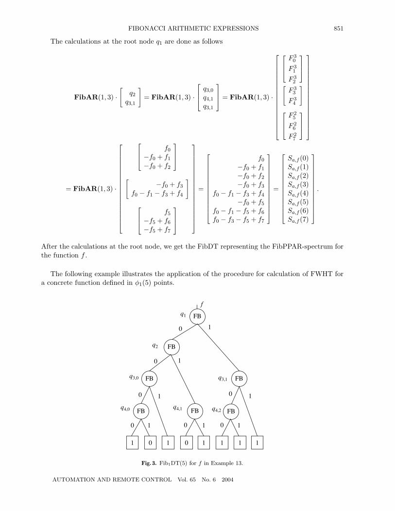
The calculations at the root node q1 are done as follows

FibAR(1, 3) ·[

q2

q3,1

]= FibAR(1, 3) ·

q3,0

q4,1

q3,1

= FibAR(1, 3) ·

F 30

F 31

F 32

[F 3

3

F 34

]

F 25

F 26

F 27

= FibAR(1, 3) ·

f0

−f0 + f1

−f0 + f2

[−f0 + f3

f0 − f1 − f3 + f4

]

f5

−f5 + f6

−f5 + f7

=

f0

−f0 + f1

−f0 + f2

−f0 + f3

f0 − f1 − f3 + f4

−f0 + f5

f0 − f1 − f5 + f6

f0 − f3 − f5 + f7

=

Sa,f (0)Sa,f (1)Sa,f (2)Sa,f (3)Sa,f (4)Sa,f (5)Sa,f (6)Sa,f (7)

.

After the calculations at the root node, we get the FibDT representing the FibPPAR-spectrum forthe function f .

The following example illustrates the application of the procedure for calculation of FWHT fora concrete function defined in φ1(5) points.

1 10 0 1 1 1 1

0 1

0

0

0

0

00 1 1

11

1

1

FB

FBFBFB

FB

FB

FB

q

4,0

q

3,0

q

2

q

1

q

3,1

q

4,2

q

4,1

f

Fig. 3. Fib1DT(5) for f in Example 13.


852 ASTOLA et al.

0

q

2

f

0

0

0 1 1 1

1

1

1

1

0 0

0

FB

FB

FB

FB FB FB

FB

1 –1 1 000 2

FibAR(1,3)

FB

FB

FB FB

0

0

0

0

1

1

1 1

01 2

q

3,1

FBFB

q

3,0

FibAR(1,3)

1

10

0 0

0 1

1

01 1 10

FBFB

FibAR(1,3) FibAR(1,3)

FB

1

10

q

4,0

0

FB

10

10

q

4,1

FB

1

10

q

4,0

0

–1

–1 –1

–1

–1 –1

Fig. 4. Calculation of FibAR-spectrum for f in Example 13.

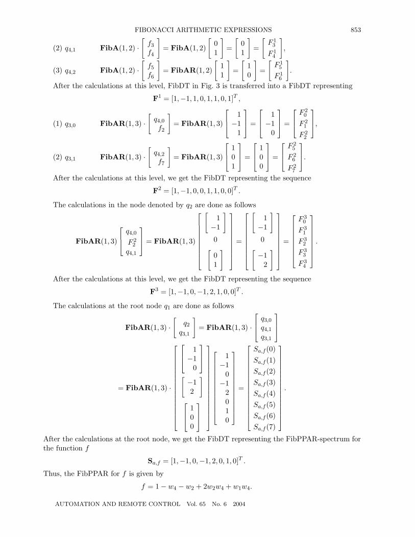
Example 13. Consider the function f given by the truth-vector F = [1, 0, 1, 0, 1, 1, 1, 1]T . Fig-ure 3 shows FB1DT(5) for f . Figure 4 illustrates the calculation of the FibAR-spectrum for fthrough processing of nodes in this FibDT. In this example, the calculation goes as follows

(1) q4,0 FibA(1, 2) ·[

f0

f1

]= FibAR(1, 2) ·

[10

]=

[1

−1

]=

[F 1

0

F 11

],



(2) q4,1 FibA(1, 2) ·[

f3

f4

]= FibA(1, 2)

[01

]=

[01

]=

[F 1

3

F 14

],

(3) q4,2 FibA(1, 2) ·[

f5

f6

]= FibAR(1, 2)

[11

]=

[10

]=

[F 1

5

F 16

].

After the calculations at this level, FibDT in Fig. 3 is transferred into a FibDT representing

F1 = [1,−1, 1, 0, 1, 1, 0, 1]T ,

(1) q3,0 FibAR(1, 3) ·[

q4,0

f2

]= FibAR(1, 3)

1−11

=

1−10

=

F 20

F 21

F 22

,

(2) q3,1 FibAR(1, 3) ·[

q4,2

f7

]= FibAR(1, 3)

101

=

100

=

F 25

F 26

F 27

.

After the calculations at this level, we get the FibDT representing the sequence

F2 = [1,−1, 0, 0, 1, 1, 0, 0]T .

The calculations in the node denoted by q2 are done as follows

FibAR(1, 3)

q4,0

F 22

q4,1

= FibAR(1, 3)

[1

−1

]

0[01

]

=

[1

−1

]

0[−12

]

=

F 30

F 31

F 32

F 33

F 34

.

After the calculations at this level, we get the FibDT representing the sequence

F3 = [1,−1, 0,−1, 2, 1, 0, 0]T .

The calculations at the root node q1 are done as follows

FibAR(1, 3) ·[

q2

q3,1

]= FibAR(1, 3) ·

q3,0

q4,1

q3,1

= FibAR(1, 3) ·

1−10

[−12

]

100

1−10

−12010

=

Sa,f (0)Sa,f (1)Sa,f (2)Sa,f (3)Sa,f (4)Sa,f (5)Sa,f (6)Sa,f (7)

.

After the calculations at the root node, we get the FibDT representing the FibPPAR-spectrum forthe function f

Sa,f = [1,−1, 0,−1, 2, 0, 1, 0]T .

Thus, the FibPPAR for f is given by

f = 1− w4 − w2 + 2w2w4 + w1w4.


854 ASTOLA et al.

6. CLOSING REMARKS

Different bit-level and word-level expressions for switching functions and related decision dia-grams are standard tools in CAD systems for systems design by referring to the Boolean intercon-nection topologies. The Fibonacci interconnection topologies are recently offered as an alternativepermitting to overcome some restrictions inherent in Boolean topologies. With this motivation,in this paper we extended the arithmetic expressions for switching functions to functions used inFibonacci interconnection topologies. It is believed that these expressions and decision diagramswill provide a base for a wider use of Fibonacci topologies and to exploit in practice the advantagesthey provide.

The wavelets-like recursive structure of the Fibonacci arithmetic transform matrices provides abasis for derivation of efficient calculation algorithms for FibARs.

ACKNOWLEDGMENTS

This paper was prepared during the stay of R.S. Stankovic and M. Stankovic at Int. Center forSignal Processing at Tampere University of Technology (TICSP). The support and the facilitiesprovided by the TICSP are gratefully appreciated and acknowledged.

APPENDIX

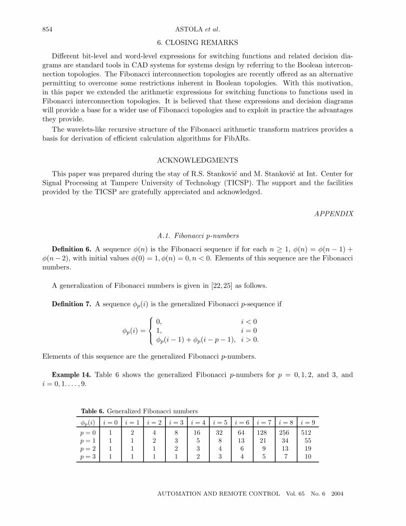
A.1. Fibonacci p-numbers

Definition 6. A sequence φ(n) is the Fibonacci sequence if for each n ≥ 1, φ(n) = φ(n − 1) +φ(n− 2), with initial values φ(0) = 1, φ(n) = 0, n < 0. Elements of this sequence are the Fibonaccinumbers.

A generalization of Fibonacci numbers is given in [22,25] as follows.

Definition 7. A sequence φp(i) is the generalized Fibonacci p-sequence if

φp(i) =

0, i < 01, i = 0φp(i − 1) + φp(i − p − 1), i > 0.

Elements of this sequence are the generalized Fibonacci p-numbers.

Example 14. Table 6 shows the generalized Fibonacci p-numbers for p = 0, 1, 2, and 3, andi = 0, 1. . . . , 9.

Table 6. Generalized Fibonacci numbers

φp(i) i = 0 i = 1 i = 2 i = 3 i = 4 i = 5 i = 6 i = 7 i = 8 i = 9

p = 0 1 2 4 8 16 32 64 128 256 512p = 1 1 1 2 3 5 8 13 21 34 55p = 2 1 1 1 2 3 4 6 9 13 19p = 3 1 1 1 1 2 3 4 5 7 10



A.2. Fibonacci p-codes

The Fibonacci p-representation of a natural number B is defined as

B =n−1∑i=p

aiφp(i).

The sequence a = (an−1, . . . , ap)p is the Fibonacci p-code for B [25]. Since with thus definedweighting coefficients, a given number B may be represented by few different code sequences, thenormal unique Fibonacci p-code is introduced by the requirement

B = φp(n − 1) + m,

where φ(n−1) is the greatest Fibonacci p-number smaller or equal to B, and 0 ≤ m < φp(n−p−1).

A.3. Contracted Fibonacci p-codes

The following property of normal Fibonacci p-codes permit definition of the contracted Fibonaccip-codes.

Lemma 1 ([25]). In the normal Fibonacci p-code for a given number B, if ai = 1, then ai−1 =ai−2 = . . . = ai−p = 0.

Utilizing this property, the contracted Fibonacci p-code is defined by deleting p zeros after each 1in the Fibonacci p-code for B, except for the rightmost 1, in which case we should delete max(i, p)zeros where there are i zeros to the right of the rightmost 1.

REFERENCES

1. Komamiya, Y., Theory of Relay Networks for the Transformation between the Decimal and BinarySystem, Bull. of E.T.L., 1951, vol. 15, no. 8, pp. 188–197.

2. Komamiya, Y., Theory of Computing Networks, Proc. of the First National Congr. for Applied Mathe-matics , 1952, pp. 527–532.

3. Komamiya, Y., Theory of Computing Networks, Researchers of the Applied Mathematics Section ofElectrotechnical Laboratory in Japanase Government , 2 Chome, Nagata-cho, Chiyodaku, Tokyo, 1959,p. 40.

4. Sintez elektronnykh vychislitel’nykh i upravlyayushchikh skhem (Synthesis of Electronic Calculation andControl Networks), Moscow: Inostrannaya Literatura, 1954.

5. Malyugin, V.D., Parallel’nye logicheskie vychisleniya posredstvom arifmeticheskikh polinomov (ParalleledCalculation by Means of Arithmetic Polynomials), Moscow: Nauka, 1997.

6. Sasao, T., Switching Theory for Logic Synthesis , New York: Kluwer, 1999.

7. Kukharev, G.A., Shmerko, V.P., and Yanushkievich, S.N., Tekhnika parallel’noi obrabotki binarnykhdannykh na SBIS (Techniques of Binary Data Parallel Procesing for VLSI), Minsk: Vysheyshaja Shcola,1991.

8. Malyugin, V.D., Kukharev, G.A., and Shmerko, V.P., Proobrazovaniya polinomial’nykh form bulevykhfunktsii (Transforms of Polynomial Forms of Boolean Functions), Moscow: Inst. Probl. Upravlen., 1986,pp. 1–48.

9. Malyugin, V.D., On a Polynomial Realization of a Cortege of Boolean Functions, Dokl. Akad. NaukSSSR, 1982, vol. 265, no. 6.


856 ASTOLA et al.

10. Moraga, C., Advances in Sepctral Techniques, Berichte zur angewandten Inforamtik , Universitat Dort-mund, 1998.2, ISSN 0946-2341.

11. Representations of Discrete Functions , Sasao, T. and Fujita, M., Eds., New York: Kluwer, 1996.

12. Sasao, T., Representations of Logic Functions by using EXOR Operators, in [11], pp. 29–54.

13. Stankovic, R.S., Some Remarks about Spectral Interpretation of MTBDDS and EVBDDs, Proc. ASP-DAC’95 , Makuhari Messe, Chiba, Japan, 1995, pp. 385–390.

14. Stankovic, R.S., Spectral Transform Decision Diagrams in Simple Questions and Simple Answers, Bel-grade: Nauka, 1998.

15. Stankovic, R.S., Sasao, T., and Moraga, C., Spectral Transform Decision Diagrams, in Representationsof Discrete Functions , Sasao, M. and Fujita, M., Eds., Norwell: Kluwer, 1996, pp. 55–92.

16. Stankovic, R.S., Functional Decision Diagrams for Multiple-valued Functions, Proc. 25th Int. Symp. onMultiple-Valued Logic, Bloomington, Indiana, USA, 1995, pp. 284–289.

17. Drechsler, R. and Becker, B., Binary Decision Diagrams, Theory and Implementation, New York:Kluwer, 1998.

18. Falkowski, B.J. and Cahng, C.H., Properties and Methods of Calcualtion Generalized Arithmetic andAdding Transforms, IEE Proc. Circuits, Devices, Syst., 1997, vol. 144, no. 5, pp. 249–258.

19. Falkowski, B.J. and Chang, C.H., Mutual Conversions between Generalized Arithmetic and Free BinaryDecision Diagrams, IEE Proc. Circuits, Devices, Syst., 1998, vol. 145, no. 4, pp. 219–228.

20. Stankovic, R.S. and Sasao, T., Decision Diagrams for Representation of Discrete Functions: UniformInterpretation and Classification, Proc. ASP-DAC’98 , Yokohama, Japan, 1998.

21. Agaian, S., Astola, J., and Egiazarian, K., Binary Polynomial Transforms and Nonlinear Digital Filters,New York: Marcel Dekker, 1995.

22. Stakhov, A.P., Algorithmic Measurement Theory, Znanie, 1979, no. 6.

23. Egiazarian, K. and Astola, J., Discrete Orthogonal Transforms Based on Fibonacci-type Recursion, Proc.IEEE Digital Signal Processing Workshop (DSPWS-96), Norway, 1996.

24. Egiazarian, K., Gevorkian, D., and Astola, J., Time-varying Filter Banks andMultiresolution TransformsBased on Generalized Fibonacci Topology, Proc. 5th IEEE Int. Workshop on Intelligent Signal Proc.and Communication Systems , Kuala Lumpur, Malaysia, 1997, S16.5.1–S16.5.4.

25. Egiazarian, K., Astola. J., and Agaian, S., Orthogonal Transforms Based on Generalized FibonacciRecursions, Proc. 2nd Int. Workshop on Spectral Techniques and Filter Banks, Brandenburg, Germany,1999.

26. Egiazarian, K. and Astola, J., On Generalized Fibonacci Cubes and Unitary Transforms, Appl. AlgebraEng. Commun. Computing, 1997, vol. AAECC 8, pp. 371–377.

27. Agaian, S., Astola, J., Egiazarian, K., and Kuosmanen, P., Decompositional Methods for Stack Filteringusing Fibonacci p-codes, Signal Processing, 1995, vol. 41, no. 1, pp. 101–110.

28. Akers, S.B., Binary Decision Diagrams, IEEE Trans. Computers , 1978, vol. C-27, no. 6, pp. 509–516.

29. Bryant, R.E., Graph-based Algorithms for Boolean Functions Manipulation, IEEE Trans. Computers ,1986, vol. C-35, no. 8, pp. 667–691.

30. Clarke, E.M., McMillan, K.L., Zhao, X., and Fujita, M., Spectral Transforms for Extremely LargeBoolean Functions, in Proc. IFIP WG 10.5 Workshop on Applications of the Reed–Muller Expressionin Circuit Design, Hamburg, 1993, pp. 86–90.

31. Stankovic, R.S., Stankovic, M., Astola, J.T., and Egiazarian, K., Fibonacci Decision Diagrams and Spec-tral Fibonacci Decision Diagrams, Proc. 30th Int. Symp. on Multiple-Valued Logic, Portland, Oregon,USA, 2000, pp. 206–211.

This paper was recommended for publication by P.P. Parkhomenko, a member of the EditorialBoard


Fibonacci arithmetic expressions

Documents

Transcript of Fibonacci arithmetic expressions