THE ARITHMETIC OF DISCOUNTING

PETER R. KILLEEN

ARIZONA STATE UNIVERSITY

Most current models of delay discounting multiply the nominal value of a good whose receipt is delayed,by a discount factor that is some function of that delay. This article reviews the logic of a theory thatdiscounts the utility of delayed goods by adding the utility of the good to the disutility of the delay. Inlimiting cases it approaches other familiar models, such as hyperbolic discounting. In nonlimit cases itmakes different predictions, generally requiring, inter alia, a magnitude effect when the value of goods isvaried. A different theory is proposed for conditioning experiments. In it utility is computed as the averagereinforcing strength of the stimuli that signal the delay. Both theories are extended to experiments inwhich degree of preference is measured, rather than adjustment to iso-utility values.Key words: additive utilities, adjusting procedure, delay discounting, magnitude effect, preference

procedure

All popular models of delay discountingassume that a proper covering model computesthe current value of a delayed good by multi-plying the amount to be discounted by somefraction that is a function of time: vDisc¼ vNomf(d), where vDisc is the current discountedvaluation of a good that will be delivered inthe future, vNom is the nominal value of thegood—the value that it would have if deliveredimmediately—and f(d) is some function of d, thedelay interval. Classic instances of f(d) areexponential, hyperbolic, and hyperbolic-powerfunctions of time, all seen in this journal issue.This preference for a multiplicative form

undoubtedly stems from the interest ratescharged or bequeathed by banks, which mustprovide some measure of scale invariance: Theproportional discount, PDisc¼ vDisc / vNommustbe independent of the dollar value of thedeferred good. If for some fixed period of timePDisc¼ 0.5, then vDisc(100)¼ 50; vDisc(1000)¼500, and so on. There is no magnitude effect: Thediscount factor is f(d), not f(d, vNom). If therewere a magnitude effect—say, that largevNom were discounted at lower rates thansmaller ones—then an individual or associationcould make a profit by consolidating loans andreceiving a better rate from the bank, part ofwhich savings the financier would pocket. Inlike manner, if banks did not use the exponen-

tial discount function, it would again bepossible to make money-pumps out of them.In this case, the financier would manage debtsin time, rather than amount. If, for instance,banks used hyperbolic discounting, the finan-cier would profit by marketing slowly dis-counted long-term debt against highlydiscounted short-term debt. Although suchoptions are common in the stock market wherevalues fluctuate moment-to-moment, banksmust guarantee a fixed return on investment.The only discount function whose rate isindependent of time is the exponential func-tion. Market forces would quickly drive hyper-bolic bank rates toward the exponential.Another historic influence on the choice of

multiplicative functions has been the econo-mists’ and game theorists’ models of expectedvalue for probabilistic discounting (e.g., Tver-sky & Kahneman, 1992; Von Neumann &Morgenstern, 2007). The use of a formanalogous to the standard one for delaydiscounting [viz., vDisc¼ vNom f(p)] persistsdespite the many paradoxes that arise fromsuch computations of expected value andexpected utility (Allais, 1979; Schoemaker,1982; Segal, 1987; Harless & Camerer, 1994).The constraints on brain and behavior are

not the same as the constraints on banks. Theevolutions of all are particular to their niches. Ittherefore makes some sense to liberalize ourintuitions, letting the nature of the models ofhuman behavior diverge from those normativefor banks and economic theory. Whereas thereare infinite numbers of ways we may posit more

Address correspondence to Peter R. Killeen.(e-mail: killeen@asu.edu)doi: 10.1002/jeab.130

JOURNAL OF THE EXPERIMENTAL ANALYSIS OF BEHAVIOR 2015, 103, 249–259 NUMBER 1 (JANUARY)

249

complex models for human behavior (see, e.g.,Doyle, 2013), there are only a few ways that theymight be simpler. In particular, consider thehypothesis that humans do not multiply thevalue of a good by a function of its psychologicaldelay. Instead, humans form a notion of theutility of a good, and they form a notion of thedisutility of waiting a certain length of time forit, and simply add those two.

On the one hand this may seem like astupid suggestion, as the dimensional units donot seem to be the same, and numbers couldgo negative, and isn’t it like adding applesand oranges? It couldn’t work. On the otherhand, have you ever noticed how increasingthe jackpot payoff on lotteries increases thenumber of purchasers far beyond the lot-teries’ expected value? This could not happenif the gamblers were rational and computedexpected value. We shake our heads at theirinnumeracy; but perhaps it is our models ofrationality that we should be shaking ourheads at. If humans operated according to anadditive function on probability and amount,the huge utility of the megamillions theymight win could easily overwhelm the additivedisutility of the small probability of getting it.Pascal’s middle-aged wager (Pascal’s Wager,2014)—to give up the fast life because, ifthere is even a snowball’s chance in hell ofgoing to heaven, then heaven’s infinite valuewas worth the gamble—might make somesense if he was adding utilities; but much lessif computing expected value. To infer thatgamblers are benighted because they do notadhere to our standards of rational man, orthat because one class of people has steeperdiscount functions than another—that theyare impulsive—short-changes our opportunityfor understanding what they value and howthey make trade-offs. Gamblers knowingly payto play; and sometimes smaller–sooner reallyis better; just think back to when you weren’tmiddle-aged.

Doing the NumbersHow to make this work? To add numbers,

they must have the same dimensions. It is a longtradition in psychophysics to recognize thatanimals process stimuli in ways that are typicallynonlinear functions of their magnitude. Dou-bling the energy of a light or intensity of a tonedoes not double their brightness or loudness.Power transformations provide a standard and

flexible scheme for recoding stimulus magni-tude. Let us see how this works for the utility ofmoney.

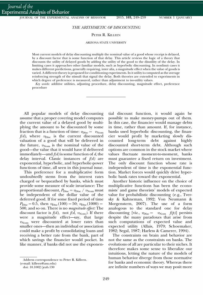
Twice as much of a thing is seldom twice asgood. Certainly it could be the case that twice asmuch money as you have in your pocket mightbe just what you need to get in to the show, andthen it might be more than twice as good. Buttwice as many bananas as you bought todaywould just go brown, twice as much sugar wouldmake your coffee too sweet, and twice as muchsupper would just make you sick. Twice as muchincome would be very good indeed; but would itbe twice as good? Would it make you exactlytwice as happy? The curve that relates delight todollars is called a utility function.

The utility of a good (a commodity) such asthe types used in delay-discounting studiestypically have the property called decreasingmarginal utility. Twice as much of the thingmakes you somewhat less than twice as happy.Here marginal means the derivative, the slopesof the curves in Figure 1, where the utility—think goodness—of a commodity is plotted onthe y-axis, and its nominal value on the x-axis.The slopes of the two curves (their derivatives)decrease with increasing values of the abscissae.In this paper I refer to the x-axis as value, andmeasure it in terms of dollar-value. The name ofthe units for utilities is utiles, which throughhappenstance rhymes with smiles. The straightline has a slope of 1/2: the rate of change in U(x)as a function of x is simply k¼ 1/2. It is constantfor all values of x and thus exemplifies constantmarginal utility. The first curved function below

Fig. 1. Exemplary utility functions for money.

250 PETER R. KILLEEN

it is U(x)¼ √kx. The margin—the derivative ofutility as a function of x—is 1/2 √(k/x). Themarginal utility is decreasing: The slope getsflatter as a function of x, decreasing proportion-ately less as x gets larger (as the inverse squareroot of x in this case). The bottom function islogarithmic: U(x)¼ ln(kx). Its derivative is 1/x,so more of a thing gets better at an even slowerrate.The linear utility function is the one implic-

itly assumed in the vast majority of delaydiscounting studies, which discount dollarvalue. The second was proposed almost 300years ago by Cramers as the utility function formoney (Pulskamp, 2013). It is consistent withthe idea that the utility of new money increasesas an inverse function of the utility of themoneythat we already have. The logarithmic functionis consistent with Bernoulli’s supposition thatutility grows in inverse proportion to the amountof money that we already have. It is the mostextrememarginal discounting that we are likelyto encounter, so forms the lower bound onplausible utility functions. Power functionsconverge on the logarithmic function as thepower approaches 0.We can represent these functions in general

asU(v)¼ (kv v)a. The powera (alpha) is 1 in thecase of linear discounting, 1/2 in the case ofCramer discounting, and approaches zero inthe case of logarithmic discounting. Thecoefficient kv is necessary because value maybe measured in many units—cents, dollars,Euros, pounds—but the utility of four quartersshould not be very different from the utility ofone dollar bill. This coefficient kv has units ofper ¢ or per $, etc.The functions shown in Figure 1 are not just

hypothetical. Usingmagnitude estimation tech-niques, Galanter (1962) found the power of theutility function for money to be around 0.4.Harinck and associates (Harinck, Van Dijk, VanBeest, & Mersmann, 2007) used categoryscaling to estimate the happiness resultingfrom finding money, and their data wereconsistent with a power function having anexponent of 0.3. Thus, the linearity assumptionunderlying traditional delay discounting tasks isempirically false. What of the assumptionunderlying the perception of time (delay) inthese tasks?A similar transformation on time is necessary:

U(t)¼ (kt t)b. The estimation of elapsed time

over small intervals is a power function with

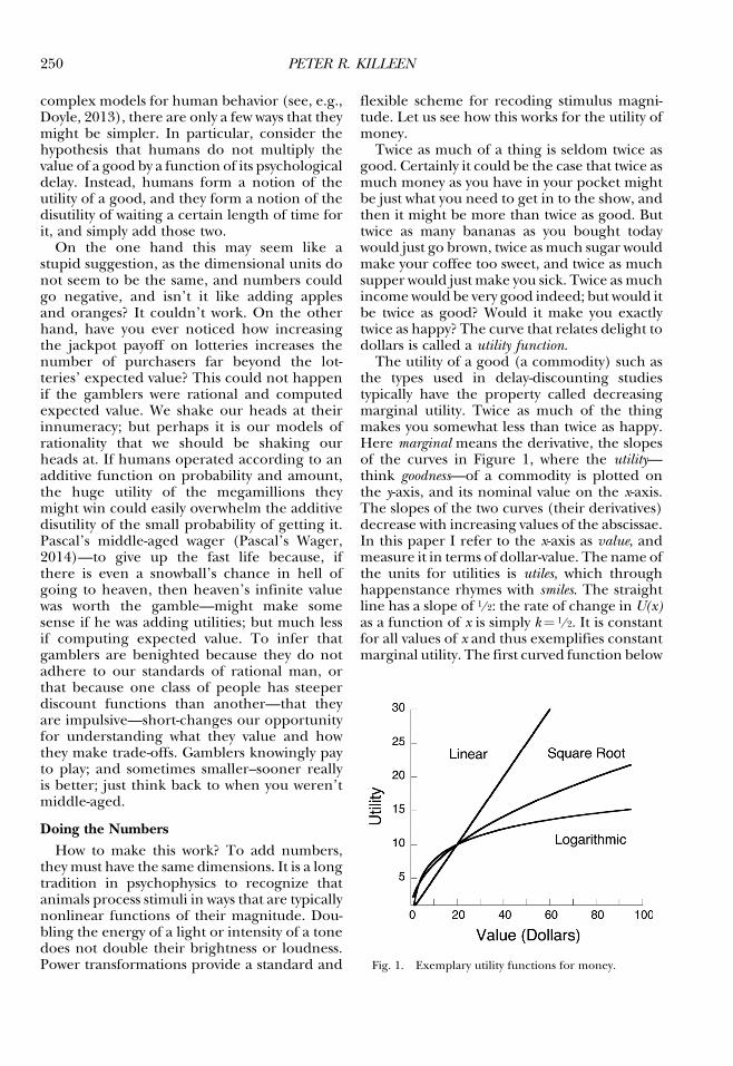
exponent just under 1 (Eisler, 1976; Allan,1983). But when dealing with estimates offuture-time over much longer intervals, theexponent shrinks. The difference betweentoday and a week from now is psychologicallylarger than the difference between 40 and 41weeks from now. In an experiment in thecontext of delay discounting, Zauberman andassociates (Zauberman, Kim, Malkoc, & Bett-man, 2009) had subjects scale the perceivedmagnitude of future times, and reported thedata shown in Figure 2.Adding it all up. According to our additive

utility hypothesis, the utility of a good with anominal value of v delivered at time t, U(v, t), isthe weighted combination of these functions onamount and delay.

U v; tð Þ ¼ w kvvð Þa− 1−wð Þ kt tð Þb ð1Þ

The parameter w is the weight that theindividual places on the utility of the good, incomparison to the disutility of waiting (0 < w <1). Some people may be more patient, or morefocused on the value of the good (largew);others may be on a tighter time schedule orplace lower value on the good (smallw).Because a delay in receiving a good is adisutility, the second term in Equation 1subtracts from the utility of the good. Consider

Fig. 2. Magnitude estimates of psychological distance tofuture dates. Data are from Zauberman and associates(2009). The curve is a power function with exponentb¼ 0.25.

ADDING UTIITIES 251

two instances of Equation 1. In the first thevalue is called vNom, delivered at a delay of t¼ d;in the second it is called vDisc and is delivered ata delay of t¼ 0:

U vNom; dð Þ ¼ w kvvNomð Þa− 1−wð Þ kt dð Þb

U vDisc; 0ð Þ ¼ w kv vDiscð Þa

The adjusting-amount procedure varies thevalue of vDisc until the subject is indifferentbetween these two utilities. (It is also possible toadjust the delay to the deferred good with afixed value for the immediate good [e.g., Greenet al., 2007; Holt, 2007]; those models are left asan exercise for the student.) Wemay model thisindifference as equality between the twoutilities:

substituting,

w kv vDiscð Þa ¼ w kv vNomð Þa− 1−wð Þ kt dð Þb

On the right is the current utility of the deferredgoodwhose street value is vNom.On the left is theutility of the good delivered immediately, whosevaluevDischasbeenadjusteduntil itsutilityequalsthat of the deferred good. It is dollar value,however, not utilities that are measured in allexperiments. To compute what those must be,divide each side by the coefficients wkv

a:

vaDisc ¼ vaNom−kdb ð2Þ

The coefficient k compacts a combination ofthe coefficients from Equation 1:

k ¼ 1−wð Þw

kbtkav

ð3aÞ

This is convenient, as estimation of theconstituent parameters would be difficult.Equation 3a makes clear that the rate ofdiscounting the utility of a delayed good, k,represents the relative weight on time com-pared to that on the good in question, alongwith some arbitrary scale factors associated withthe units in which the variables are represented.In the case that the right-hand side of Equation2 is negative, there is no immediate amount thatis small enough, and the offer is rejected.

The original derivation of this theory in-cluded the powers as coefficients of k (Eq. 3b).It remains an empirical question which version

will provide the most parsimonious account ofindividual differences by rendering the param-eters more orthogonal. (I’m betting on 3b).

k ¼ 1−wð Þw

kbtkav

a

bð3bÞ

Finally, to deliver the prediction in terms ofthe currency of the experiment, raise eachside of Equation 2 to the power 1/a (keepinga > 0):

vDisc ¼ vaNom−kdb

� �1=a ð4Þ

This is the key equation of the additive utilitymodel. In the case that the disutility of waitingexceeds the utility of the nominal amountoffered, then vDisc¼ 0.

As the value of a approaches 0, the power-utility function for the goodmay be representedby a power series (see Appendix). In that case,and invoking Equation 3b for the expansion ofk, Equation 4 may be written as:

vDisc ¼ vNome−k0db ð5Þ

The series expansion of this exponential (seeAppendix) is the familiar:

vDisc ¼ vNom

1þ k0dbð6Þ

This traditional form is thus consistent with avery concave or logarithmic utility function formoney, and its additive combination with thedisutility of delay. Because the utility of thegood does not enter Equations 5 and 6, they areuseful whenever value is not independentlyvaried along with delay, giving the same resultsas Equation 4 (with changes in the parametervalues), but saving the now redundant param-eter a. The rates of discounting in Equations 5and 6 are independent of vNom, so they predictno magnitude effect. This derivation of thehyperboloid predicts that the rate of decay k’will be inversely proportional to the power b(see Appendix).

Equation 5 is interesting because it returnsthe bankers’ discount function, corrected fornonlinearity in the future-time function. It hasbeen suggested as a discountingmodel by Ebertand Prelec (2007). It restores bankers’ ration-ality to discounting decisions if we assume a

252 PETER R. KILLEEN

steeply curved utility function for money a! 0,and a nonlinear valuation of future-time. Theirarticle is interesting because it demonstrateshow the temporal discount function (in partic-ular, the value of b) is readily subject tomanipulation. We may infer that some of thelarge heterogeneity in discounting that is foundin typical studies may be due to idiosyncraticallyperturbed future perspectives of the subjects(term papers or rents imminent in one case, anendless summer lying ahead in another). If so,standard framing instructions may help controlthis unwonted variability. Alternatively, usingexisting techniques (see, e.g., Zauberman et al.,2009), future perspective might be measuredand used as a covariate.According to the additive discount model of

Equation 4, the apparent rate of discountingwill depend on the magnitude of the value thatis discounted. Imagine discounting a good oflarge value where vaNom � kdb. Then theadditive temporal disutility would be relativelynegligible, and discounted value would essen-tially equal the nominal value. The utility ofheaven is essentially the same whether it comesin days or in decades. For the same reason thestate of the planet 100 years from now is sodistant that no economic models with sensibleexponential discount rates would counsel ex-pending many resources abating climatechange today (Dasgupta, 2006). But there aresome individuals for whom the utility of a viableplanet for their children’s children is so greatthat reductions in carbon emission are of focalimportance despite their deferred payoff. Thismakes sense in the additive model, withoutinvoking the issue of intergenerational equity(Portney & Weyant, 1999). Conversely, forgoods of little value time becomes of theessence, with any delay deadly to the enterprise.

The Problem of Scale InvarianceAll standard discounting models of the form

vDisc¼ vNom f(d) are scale invariant over thenominal value: They must predict discountingat the same rate for all values. When the delayvDisc is 0, then the proportional value of thenominal good as a function of delay isPDisc¼ vDisc / vNom¼ f(d), for all vNom. This is

also true of Equations 5 and 6. This is counter tothe facts of humandelay discounting, so all suchmodels must deal with that invalidation by adhoc adjustments of the discount rate k. Equa-

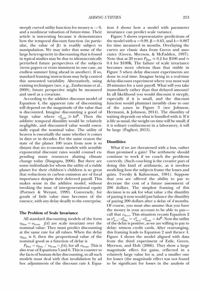
tion 4 shows how a model with parameterinvariance can predict scale variance.Figure 3 shows representative predictions of

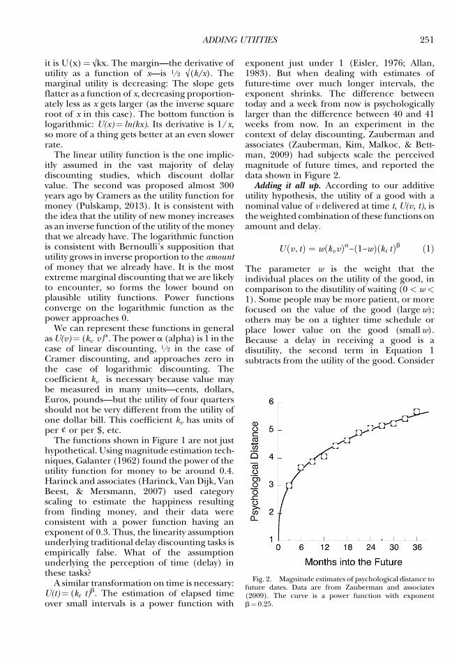
themodel with a¼ 0.09, b¼ 0.65, and k¼ 0.007for time measured in months. Overlaying thecurves are classic data from Green and asso-ciates (Green, Myerson, & McFadden, 1997).Note that at 20 years PDisc � 0.2 for $100 and �0.4 for $100K. The failure of scale invariancebecomes more obvious than that visible inFigure 3 when delay discount experiments aredone in real time. Imagine being in a real-timedelay-discount experiment where you must wait20minutes for a unit payoff. What will you takeimmediately rather than that delayed amount?In all likelihood you would discount it steeply,especially if it is small, and the discountfunction would plummet invisibly close to oneof the y-axes in Figure 3 (see Johnson,Hermann, & Johnson, 2014). The disutility ofwaiting depends on what is bundled with it: If itis life as usual, the weight on timewill be small; ifit is solitary confinement in a laboratory, it willbe large (Paglieri, 2013).

DisutilitiesWhat if we are threatened with a loss, rather

than promised a gain? The arithmetic shouldcontinue to work if we couch the problemscorrectly. (Such couching is the creative part ofdoing this kind of arithmetic, as it involvesmodeling how the subjects frame the losses andgains. Tversky & Kahneman, 1981). Supposethat you are offered the ability to pay todecrease the cost of a future assessment of200 dollars. The simplest framing of thisdecision is to ask for what value x the disutilityof paying it now would just balance the disutilityof paying 200 dollars after a delay of d months.Of course, you must also assume that you havethe money in your account to be able to pay—call that vAcct. This situation recasts Equation 2as vaAcct−v

aDisc ¼ vaAcct−v

aNom þ kdb. Now the utility

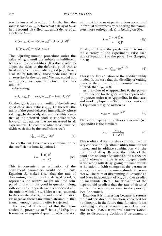
of the delay is positive, as we are willing to pay todelay: witness credit cards. After rearranging,this framing leads to Equation 2 and thence 4.Figure 4 shows the model aligned with datafrom the third experiment of Estle, Green,Myerson, and Holt (2006). They show a largemagnitude effect for gains, reflected in arelatively large value for a, and a smaller onefor losses (the magnitude effect was not foundto be significant for losses in the analysis of

ADDING UTIITIES 253

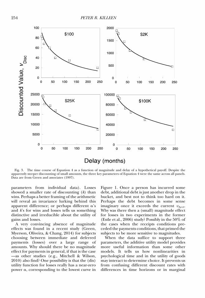
parameters from individual data). Lossesshowed a smaller rate of discounting (k) thanwins. Perhaps a better framing of the arithmeticwill reveal an invariance lurking behind thisapparent difference; or perhaps different a’sand k’s for wins and losses tells us somethingdistinctive and irreducible about the utility ofgains and losses.

A very convincing absence of magnitudeeffects was found in a recent study (Green,Myerson, Oliveira, & Chang, 2014) for subjectschoosing between immediate and deferredpayments (losses) over a large range ofamounts. Why should there be no magnitudeeffect for payments in general, if that is the case—as other studies (e.g., Mitchell & Wilson,2010) also find? One possibility is that the (dis)utility function for losses really has a near-zeropower a, corresponding to the lowest curve in

Figure 1. Once a person has incurred somedebt, additional debt is just another drop in thebucket, and best not to think too hard on it.Perhaps the debt becomes in some senseimaginary once it exceeds the current vAcct.Why was there then a (small) magnitude effectfor losses in two experiments in the former(Estle et al., 2006) study? Possibly in the 50% ofthe cases when the receipts conditions pre-ceded the payments conditions, that primed thesubjects to be more sensitive to magnitudes.

When the data suffice to support threeparameters, the additive utility model providesmore useful information than some othermodels. It tells us how nonlinearities inpsychological time and in the utility of goodsmay interact to determine choice. It prevents usfrom confusing different discount rates withdifferences in time horizons or in marginal

Fig. 3. The time course of Equation 4 as a function of magnitude and delay of a hypothetical payoff. Despite theapparently steeper discounting of small amounts, the three key parameters of Equation 4 were the same across all panels.Data are from Green and associates (1997).

254 PETER R. KILLEEN

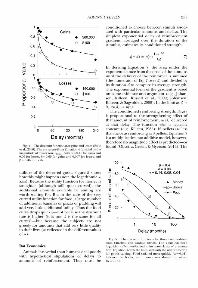
utilities of the deferred good. Figure 5 showshow this might happen (note the logarithmic x-axis). Because the utility function for money isstraighter (although still quiet curved), theadditional amounts available by waiting areworth waiting for. But in the case of the verycurved utility function for food, a large numberof additional bananas or pizzas or pudding willadd very little additional utility. Thus the foodcurve drops quickly—not because the discountrate is higher (it is not: k is the same for allcurves)—but because the subjects are notgreedy for amounts that add very little qualityto their lives (as reflected in the different valuesof a).

Rat EconomicsAnimals less verbal than humans deal poorly

with hypothetical stipulations of delays toamounts of reinforcement. They must be

conditioned to choose between stimuli associ-ated with particular amounts and delays. Thesimplest exponential delay of reinforcementgradient, averaged over the duration of thestimulus, estimates its conditioned strength:

s v; dð Þ / u vð Þ 1−e−kd

kdð7Þ

In deriving Equation 7, the area under theexponential trace from the onset of the stimulusuntil the delivery of the reinforcer is summed(the numerator of Eq. 7 over k) and divided byits duration d to compute its average strength.The exponential form of the gradient is basedon some evidence and argument (e.g., Johan-sen, Killeen, Russell et al., 2009; Johansen,Killeen, & Sagvolden, 2009). In the limit as d!0, s(v,d) ! u(v).The conditioned reinforcing strength, s(v,d),

is proportional to the strengthening effect ofthat amount of reinforcement, u(v), deliveredat that delay. The function u(v) is typicallyconcave (e.g., Killeen, 1985): 16 pellets are lessthan twice as reinforcing as 8 pellets. Equation 7is a multiplicative, not additive model, however,therefore no magnitude effect is predicted—orfound (Oliveira, Green, & Myerson, 2014). TheFig. 4. The discount functions for gains and losses (Estle

et al., 2006). The curves are fromEquation 4 (divided by themagnitude of loss or win, vNom), with a¼ 0.16 for gains and0.06 for losses, k¼ 0.65 for gains and 0.007 for losses, andb¼ 0.46 for both.

Fig. 5. The discount functions for three commodities,from Charlton and Fantino (2008). The x-axis has beenlogarithmically transformed to increase clarity of presenta-tion. Equation 4 drew the lines, with only the utility functionfor goods varying. Food satiated most quickly (a¼ 0.04),followed by books, and money was slowest to satiate(a¼ 0.14).

ADDING UTIITIES 255

discount parameter k is a measure of thesteepness of the delay of reinforcement gra-dient. The curves drawn by Equation 7 areindistinguishable from those drawn by Equa-tion 6 (Killeen, 2011 Eqs. 2 & 3). Equation 7places all the emphasis on the conditionedreinforcement strength of the stimulus signal-ing the options, but for nuance, the role ofdirect reinforcement of the choice response bythe delayed primary reinforcer may be takeninto account (Killeen, 2011).

PreferenceSome experiments use a different paradigm

to assay delay discounting: They measure theproportion of responses for one good overanother without adjusting to indifference. Thisyields a very different dependent variable.There is no reason that degree of preferenceshould follow a hyperbolic function, or even arelative measure of strength (despite somemisguided suggestions that it should, e.g.,Killeen, 2011). If I repeatedly gave you thechoice between $100 and $200 I would be quitesurprised if you chose the larger amount only2/3 of the time. If I repeatedly gave you thechoice between $100 and $120 I would be atleast as surprised if you chose the larger amountonly 55% of the time. Animals should alwayschoose what they most prefer, assuming thatthey can make that judgment. But concurrentreinforcement schedules, in which degree ofpreference is routinelymeasured, is a confusingsituation. Entering such a situation, clear andnear-exclusive preferences are soon degraded(Crowley & Donahoe, 2004). How to apply thearithmetic of discounting here? It is worthassaying a classic off-the-shelf model of con-fusion, Thurstone scaling (Thurstone, 1927)incorporated into signal detection theory as itsfoundational model. Other models of scheduleconfusion are available (e.g., Nevin, 1981) andworth exploring.

Thurstone’s confusion model represents theutility of packages of goods and delays not asexact values, but as distributions around amean. Adjustment procedures titrate someparameter so that the distributions of utilitiesof two packages of goods-plus-delays align at acommon mean. Preference procedures leavethem as two distributions on a line of utility,partially overlapping. The probability that onepackage, say, s(v1,d1) will seem better than

another, say, s(v2,d2) at themoment of choice ismost concisely given by a cumulative normaldistribution:

p O1ð Þ ¼ F s v1; d1ð Þ− v2; d2ð Þ−b;sð Þ ð8Þ

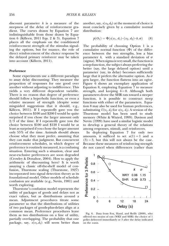
The probability of choosing Option 1 is acumulative normal function (F) of the differ-ence between the two strengths, less a biasparameter b, with a standard deviation of s(sigma).When sigma is very small, the function isa step-function, the subject always preferring thebetter (say, the large delayed option) until aparameter (say, its delay) becomes sufficientlylarge that it prefers the alternative option. As sgets larger, the function flattens into an ogive.Figure 6 shows an exemplary application ofEquation 8, employing Equation 7 to measurestrength, and keeping b¼ 0. Although bothparameters drove the SHR rats toward a steeperfunction, it is possible to construct steepfunctions with either of the parameters. Equa-tion 8 may also be used for human preferences,substituting U(vi, di) for s(vi, di). A version of theThurstone model has been used to studymemory (White & Wixted, 1999). Davison andNevin (1999) have used a similar logistic modelto develop a general theory of the relationsamong responses, stimuli, and reinforcers.

In deploying Equation 7 for only twoamounts, it sufficed to set u(1)¼ 1 and u(3)¼ 3, but this will not always be the case.Because these measures of reinforcing strengthdo not cancel when differences (rather than

Fig. 6. Data from Fox, Hand, and Reilly (2008), whooffered two strains of rats (WKY and SHR) the choice of 1pellet delivered immediately or 3 after the delay indicatedon the x-axis.

256 PETER R. KILLEEN

ratios) are taken, there will be a kind ofmagnitude effect found with this model. Dou-bling both amounts will move the distributionsapart (akin to reducing s) so that preferenceson either side of the indifference point will getmore extreme. It is notable that all of thereports of magnitude effects (or reverse magni-tude effects) with rats used the preferenceparadigm (Oliveira et al., 2014; Table 3),whereas there was no evidence of magnitudeeffects in nonverbal animals using the adjust-ment paradigm.

Discussion

Arithmetic is relatively easy, but decidingwhat to add requires a sense of how theorganism evaluates the options available to it,and how thosemight be affected by the framingof the experimental paradigm. It requiresexperimentation with the math, as much aswith the rats. Therefore all of the above modelsshould be viewed as hypotheses. The readers areinvited to do their own sums. In addition theymight test some of the qualitative predictions ofthis simple but strange approach, some of whichare found in Killeen (2009). Serious evaluationof the models requires analyses of data fromindividual subjects, as averaging curvilinearfunctions can mislead. Green, Myerson, andtheir collaborators provide many examples ofthe proper ways to analyze such data.

Appendix

The limit as a ! 0.Restating Equation 2:

vaDisc ¼ vaNom−kdb ðA1Þ

The Maclaurin series expansion of va is(Burington, 1948 p. 44):

va ¼ 1þ alnðvÞ þ ðalnðvÞÞ22!

þ ::: ðA2Þ

For small values of a all but the first two terms ofthe series may be ignored, as higher powers of aquickly become minuscule. Substituting thoseinto Equation A1:

1þ aln vDiscð Þ ¼ 1þ aln vNomð Þ−kdb ðA3Þ

Rearranging:

ln vDiscð Þ ¼ ln vNomð Þ− kadb ðA4Þ

Exponentiating:

vDisc ¼ vNome−kad

b ðA5Þ

Here is where taking Equation 3b as the properexpansion of k is useful, as the parameter alphacancels out of the exponent, avoiding divisionby zero in the limiting case:

vDisc ¼ vNome−k0db ðA6Þ

with

k0 ¼ 1−wð Þwb

kbtkav

ðA7Þ

Reducing to the hyperboloidEquation A6 may be written as:

vDisc ¼ vNom

ek0dbðA8Þ

Notice that if v in Equation A2 is e, then it maybe written as:

ea ¼ 1þ aþ a2

2!þ ::: ðA9Þ

In this case, a ¼ k0db;. Then substituting thefirst two terms for the denominator of EquationA8, that may be written as:

vDisc ¼ vNorm

1þ k0dbðA10Þ

This is the standard hyperboloid discountingfunction. Note that k’ has b in its denominator(Eq. A7). This derivation of the hyperboloidtherefore predicts that the discount rate will beinversely proportional to the exponent b�

References

Allais, M. (1979). The so-called Allais paradox and rationaldecisions under uncertainty Expected utility hypothesesand the Allais paradox (pp. 437–681). Amsterdam:Springer.

Allan, L. G. (1983). Magnitude estimation of temporalintervals. Perception and Psychophysics, 33, 29–42. doi:http://dx.doi.org/10.3758/BF03205863.

ADDING UTIITIES 257

Burington, R. S. (1948). Handbook of MathematicalTables and Formulas. Sandusky, OH: HandbookPublishers, Inc.

Charlton, S. R., & Fantino, E. (2008). Commodity specificrates of temporal discounting: does metabolic functionunderlie differences in rates of discounting? Behav-ioural Processes, 77(3), 334–342. doi: http://dx.doi.org/10.1016/j.beproc.2007.08.002.

Crowley, M. A., & Donahoe, J. W. (2004). Matching: Itsacquisition and generalization. Journal of the Experimen-tal Analysis of Behavior, 82(2), 143–159. doi: http://dx.doi.org/10.1901/jeab.2004.82–143.

Dasgupta, P. (2006). Comments on the Stern Review’seconomics of climate change. Foundation for Science andTechnology, http://econ.tau.ac.il/papers/research/Partha Dasgupta on Stern Review.pdf.

Davison, M., & Nevin, J. A. (1999). Stimuli, reinforcers andbehavior: An integration. Journal of the ExperimentalAnalysis of Behavior, 71, 439–482. doi: 10.1901/jeab.1999.71–439.

Doyle, J. R. (2013). Survey of time preference, delaydiscountingmodels. Judgment and DecisionMaking, 8(2),116–135. doi: http://dx.doi.org/10.2139/ssrn.1685861.

Ebert, J., & Prelec, D. (2007). The fragility of time: Time-insensitivity and valuation of the near and far future.Management Science, 53, 1423–1438. doi: http://dx.doi.org/10.1287/mnsc.1060.0671.

Eisler, H. (1976). Experiments on subjective duration1868–1975: A collection of power function exponents.Psychological Bulletin, 83(6), 1154. doi: http://dx.doi.org/10.1037/0033–2909.83.6.1154.

Estle, S. J., Green, L., Myerson, J., & Holt, D. D. (2006).Differential effects of amount on temporal andprobability discounting of gains and losses. Memoryand Cognition, 34, 914–928. doi: http://dx.doi.org/10.3758/BF03193437.

Fox, A. T., Hand, D. J., & Reilly, M. P. (2008). Impulsivechoice in a rodent model of attention-deficit/hyper-activity disorder. Behavioural Brain Research, 187(1),146–152. doi: http://dx.doi.org/10.1016/j.bbr.2007.09.008.

Galanter, E. (1962). The direct measurement of utility andsubjective probability. American Journal of Psychology, 72,208–220. doi: http://dx.doi.org/10.2307/1419604.

Green, L., Myerson, J., & McFadden, E. (1997). Rate oftemporal discounting decreases with amount ofreward. Memory and Cognition, 25, 715–723. doi:http://dx.doi.org/10.3758/BF03211314.

Green, L., Myerson, J., Oliveira, L., & Chang, S. E. (2014).Discounting of delayed and probabilistic losses over awide range of amounts. Journal of the ExperimentalAnalysis of Behavior, 101(2), 186–200. doi: http://dx.doi.org/10.1002/jeab.56.

Green, L., Myerson, J., Shah, A. K., Estle, S. J., & Holt, D. D.(2007). Do adjusting-amount and adjusting-delayprocedures produce equivalent estimates of subjectivevalue in pigeons? Journal of the Experimental Analysis ofBehavior, 87(3), 337–347. doi: http://dx.doi.org/10.1901/jeab.2007.37–06.

Harinck, F., Van Dijk, E., Van Beest, I., & Mersmann, P.(2007). When gains loom larger than losses: Lossaversion for small amounts of money. PsychologicalScience, 18, 1099–1105. doi: http://dx.doi.org/10.1111/j.1467–9280 .2007.02031.x.

Harless, D. W., & Camerer, C. F. (1994). The predictiveutility of generalized expected utility theories. Econo-metrica: Journal of the Econometric Society, 1251–1289. doi:http://dx.doi.org/10.2307/2951749.

Johansen, E. B., Killeen, P. R., Russell, V. A., Tripp, G.,Wickens, J. R., Tannock, R., & Sagvolden, T. (2009).Origins of altered reinforcement effects in ADHD.Behavioral and Brain Functions, 5, 7. doi: http://dx.doi.org/10.1186/1744–9081 -5–7 .

Johansen, E. B., Killeen, P. R., & Sagvolden, T. (2009).Behavioral variability, elimination of responses, anddelay-of-reinforcement gradients in SHR andWKY rats.Behavioral and Brain Functions, 3. doi: http://dx.doi.org/10.1186/1744–9081 -3–60 .

Johnson, P. S., Herrmann, E. S., & Johnson, M. W. (2014).Opportunity costs of reward delays and the discountingof hypotheical money and cigarettes. Journal of theExperimental Analysis of Behavior. Advance onlinepublication. doi: 10.1002/jeab.110.

Killeen, P. R. (1985). Incentive theory IV: Magnitude ofreward. Journal of the Experimental Analysis of Behavior, 43,407–417. doi: http://dx.doi.org/10.1901/jeab.1985.43–407.

Killeen, P. R. (2009). An additive-utility model of delaydiscounting. Psychological Review, 116, 602–619. doi:http://dx.doi.org/10.1037/a0016414.

Killeen, P. R. (2011). Models of trace decay, eligibility forreinforcement, and delay of reinforcement gradients,from exponential to hyperboloid. Behavioural Processes,8(1), 57–63. doi: http://dx.doi.org/10.1016/j.beproc.2010.12.016.

Mitchell, S. H., & Wilson, V. B. (2010). The subjectivevalue of delayed and probabilistic outcomes: Outcomesize matters for gains but not for losses. BehaviouralProcesses, 83(1), 36–40. doi: http://dx.doi.org/10.1016/j.beproc.2009.09.003.

Nevin, J. A. (1981). Psychophysics and reinforcementschedules: An integration. In M. L. Commons & J.A.Nevin (Eds.), Quantitative Analysis of Behavior: Discrim-inative Properties of Reinforcement Schedules (Vol. 1, pp. 3–27). Cambridge: Ballinger.

Oliveira, L., Green, L., & Myerson, J. (2014). Pigeons’ delaydiscounting functions established using a concurrent-chains procedure. Journal of the Experimental Analysis ofBehavior, 102(2), 151–161. doi: http://dx.doi.org/10.1002/jeab.97.

Paglieri, F. (2013). The costs of delay: Waiting versuspostponing in intertemporal choice. Journal of theExperimental Analysis of Behavior, 99, 362–377. doi:10.1002/jeab.18.

Pascal’s Wager. (2014, Nov. 10). In Wikipedia, The FreeEncyclopedia. Retrieved Nov. 20, 2014, from http://en.wikipedia.org/w/index.php?title¼Pascal%27s_Wager_oldid¼633303305.

Portney, P. R., &Weyant, J. P. (Eds.). (1999).Discounting andIntergenerational Equity. Washington, DC: Resources forthe Future.

Pulskamp, R. J. (2013). Correspondence of NicolasBernoulli concerning the St. Petersburg Game. 2007,1–9. cerebro.xu.edu/math/Sources/NBernoulli/cor-respondence_petersburg_game.pdf

Schoemaker, P. J. H. (1982). The Expected Utility Model: ItsVariants, Purposes, Evidence and Limitations. Chicago:Center for Decision Research, The University ofChicago.

258 PETER R. KILLEEN

Segal, U. (1987). The Ellsberg paradox and risk aversion:An anticipated utility approach. International EconomicReview, 28, 175–202. doi: http://dx.doi.org/10.2307/2526866.

Thurstone, L. L. (1927). A law of comparative judgment.Psychological Review, 34, 273–286. doi: http://dx.doi.org/10.1037//0033–295X.101.2.266.

Tversky, A., & Kahneman, D. (1981). The framingof decisions and the psychology of choice. Science,211, 453–458. doi: http://dx.doi.org/10.1126/science.7455683.

Tversky, A., & Kahneman, D. (1992). Advances in prospecttheory: Cumulative representation of uncertainty.Journal of Risk and Uncertainty, 5(4), 297–323. doi:http://dx.doi.org/10.1007/BF00122574.

Von Neumann, J., & Morgenstern, O. (2007). Theory ofGames and Economic Behavior (60th Anniversary Commem-orative Edition). Princeton, NJ: Princeton UniversityPress.

Whit, K. G., & Wixted, J. T. (1999). Psychophysics ofremembering. Journal of the Experimental Analysis ofBehavior, 71(1), 91–113. doi: 10.1901/jeab.1999.71–91.

Zauberman, G., Kim, B. K., Malkoc, S. A., & Bettman, J. R.(2009). Discounting time and time discounting:Subjective time perception and intertemporal prefer-ences. Journal of Marketing Research, 46(4), 543–556. doi:http://dx.doi.org/10.1509/jmkr.46.4.543.

Received: July 21, 2014Final Acceptance: November 20, 2014

ADDING UTIITIES 259