18.783 Elliptic CurvesLecture #4

Spring 201902/19/2019

4 Finite field arithmetic

We saw in Lecture 3 how to efficiently multiply integers, and, using Kronecker substitution,how to efficiently multiply polynomials with integer coefficients. This gives us what we needto multiply elements in finite fields, provided we can efficiently reduce the results to ourstandard representations of Fp ' Z/pZ and Fq ' Fp[x]/(f), using integers in [0, p − 1] andpolynomials of degree less than deg f , respectively. In both cases we use Euclidean division.

4.1 Euclidean division

Given integers a, b > 0, we wish to compute the unique integers q, r ≥ 0 for which

a = bq + r (0 ≤ r < b).

We have q = ba/bc and r = a mod b. It is enough to compute q, since we can then computer = a − bq. To compute q, we determine a sufficiently precise approximation c ≈ 1/b andobtain q by computing ca and rounding down to the nearest integer.

We recall Newton’s method for finding the root of a real-valued function f(x). Westart with an initial approximation x0, and at each step, we refine the approximation xiby computing the x-coordinate xi+1 of the point where the tangent line through (xi, f(xi))intersects the x-axis, via

xi+1 := xi −f(xi)

f ′(xi).

To compute c ≈ 1/b, we apply this to f(x) = 1/x− b, using the Newton iteration

xi+1 = xi −f(xi)

f ′(xi)= xi −

1xi− b− 1x2i

= 2xi − bx2i .

As an example, let us approximate 1/b = 1/123456789. For the sake of illustration wework in base 10, but in an actual implementation would use base 2, or base 2w, where w isthe word size.

x0 = 1× 10−8

x1 = 2(1× 10−8)− (1.2× 108)(1× 10−8)2

= 0.80× 10−8

x2 = 2(0.80× 10−8)− (1.234× 108)(0.80× 10−8)2

= 0.8102× 10−8

x3 = 2(0.8102× 10−8)− (1.2345678× 108)(0.8102× 10−8)2

= 0.81000002× 10−8.

Note that we double the precision we are using at each step, and each xi is correct up to anerror in its last decimal place. The value x3 suffices to correctly compute ba/bc for a ≤ 1015.

To analyze the complexity of this approach, let us assume that b has n bits and a hasat most 2n bits; this is precisely the situation we will encounter when we wish to reducethe product of two integers in [0, p− 1] modulo p. During the Newton iteration to computec ≈ 1/b, the size of the integers involved doubles with each step, and the cost of the arithmeticoperations grows at least linearly. The total cost is thus at most twice the cost of the last

Lecture by Andrew Sutherland

step, which is M(n) + O(n); note that all operations can be performed using integers byshifting the operands appropriately. Thus we can compute c ≈ 1/b in time 2M(n) + O(n).We can then compute ca ≈ a/b, round to the nearest integer, and compute r = a− bq usingat most 4M(n) +O(n) bit operations.

With a slightly more sophisticated version of this approach it is possible to compute r intime 3M(n) + O(n). If we expect to repeatedly perform Euclidean division with the samedenominator, as when working in Fp, the cost of all subsequent reductions can be reducedto M(n) +O(n) using what is known as Barret Reduction; see [2, Alg. 10.17].1 In any case,we obtain the following bound for multiplication in Fp using our standard representation asintegers in [0, p− 1].

Theorem 4.1. The time to multiply two elements of Fp is O(M(n)), where n = lg p.

There is an analogous version of this algorithm above for polynomials that uses the exactsame Newton iteration xi+1 = 2xi − bx2i , where b and the xi are now polynomials. Ratherthan working with Laurent polynomials (the polynomial version of approximating a rationalnumber with a truncated decimal expansion), it is simpler to reverse the polynomials andwork modulo a sufficiently large power of x, doubling the power of x with each Newtoniteration. More precisely, we have the following algorithm, which combines Algorithms 9.3and 9.5 from [3]. For any polynomial f(x) we write rev f for the polynomial xdeg ff( 1x); thissimply reverses the coefficients of f .

Algorithm 4.2 (Fast Euclidean division of polynomials). Given a, b ∈ Fp[x] with b monic,compute q, r ∈ Fp[x] such that a = qb+ r with deg r < deg b as follows:

1. If deg a < deg b then return q = 0 and r = a.

2. Let m = deg a− deg b and k = dlgm+ 1e.3. Let f = rev(b) (reverse the coefficients of b).

4. Compute g0 = 1, gi = (2gi−1 − fg2i−1) mod x2i for i from 1 to k.

(this yields fgk ≡ 1 mod xm+1).

5. Set s = rev(a)gk mod xm+1 (now rev(b)s ≡ rev(a) mod xm+1).

6. Return q = xm−deg s rev(s) and r = a− bq.

As in the integer case, the work is dominated by the last iteration in step 4, which involvesmultiplying polynomials in Fp[x]. To multiply elements of Fq ' Fp[x]/(f) represented aspolynomials of degree less than d = deg f , we compute the product a in F[x] and then reducemodulo b = f , and the degree of the polynomials involved are all O(d). With Kroneckersubstitution, we can reduce these polynomial multiplications to integer multiplications, andobtain the following result.

Theorem 4.3. Let q = pd be a prime power, and assume that either log d = O(log p) orp = O(1). The time to multiply two elements of Fq is O(M(n)), where n = lg q.

Remark 4.4. The constraints on the relative growth rate on p and d in the theorem aboveare present only so that we can easily express our bounds in terms of the bound M(n) formultiplying integers. In fact, for all the bounds currently known for M(n), Theorem 4.3

1The algorithm given in [2] for the precomputation step of Barret reduction uses Newton iteration witha fixed precision, which is asymptotically suboptimal; it is better to use the varying precision approachdescribed above. But in practice the precomputation cost is usually not a major concern.

18.783 Spring 2019, Lecture #4, Page 2

holds uniformly, without any assumptions about the relative growth rate of p and d. Moreprecisely, it follows from [5] that for any prime power q we can multiply two elements inFq in time O(n log n8log

∗n), no matter how q = pd tends to infinity; but the proof of thisrequires more than just Kronecker substitution.

Before leaving the topic of Euclidean division, we should also mention the standard“schoolbook” algorithm of long division. The classical algorithm works with decimal digits(base 10), but for the sake of simplicity let us work in base 2; in practice one works in base2w for some fixed w.

Algorithm 4.5 (Long division). Given positive integers a =∑m

i=0 ai2i and b =

∑ni=0 bi2

i,compute q, r ∈ Z such that a = qb+ r with 0 ≤ r < b as follows:

1. If b > a return q = 0 and r = b, and if b = 1 return q = a and r = 0.

2. Set q ← 0, r ← 0, and k ← m.

3. While k ≥ 0 and r < b set q ← 2q, r ← 2r + ak, and k ← k − 1.

4. If r < b then return q and r.

5. Set q ← q + 1, r ← r − b, and return to Step 3.

The net effect of all the executions of Step 3 is is to add a to qb+r using double-and-addbit-wise addition. The quantity qb + r is initially set to 0 in Step 2 and is unchanged byStep 5, so when the algorithm terminates in Step 4 we have a = qb + r and 0 ≤ r < b asdesired. If we are only interested in the remainder r we can omit all operations involving q.

For the complexity analysis we can assume that multiplication by 2 is achieved by bit-shifting and costs O(1) (consider a multi-tape Turing machine, or a bit-addressable RAM).Step 2 costs O(1), the total cost of Step 3 over all iterations is O(nm), as is the total costof Step 5 (note that q is a multiple of 2 at the start of Step 5, so computing q ← q + 1 isachieved by setting the least significant bit). This yields the following result.

Theorem 4.6. The long division algorithm uses O(mn) bit operations to perform Euclideandivision of an m-bit integer by an n-bit integer.

Remark 4.7. For m = O(n) the O(n2) complexity of long division is worse than theO(M(n)) cost of Euclidean division using Newton iteration. But when m is much largerthan n, say n = O(logm) or n = O(1), long division is a better choice. In particular, forany fixed prime p (so O(1) bits) we can reduce n-bit integers modulo p in linear time.

4.2 Extended Euclidean algorithm

We recall the Euclidean algorithm for computing the greatest common divisor of positiveintegers a and b. For a > b we repeatedly apply

gcd(a, b) = gcd(b, a mod b),

where we take a mod b to be the unique integer r ∈ [0, b− 1] congruent to a modulo b.To compute the multiplicative inverse of an integer modulo a prime, we use the extended

Euclidean algorithm, which expresses gcd(a, b) as a linear combination

gcd(a, b) = as+ bt,

18.783 Spring 2019, Lecture #4, Page 3

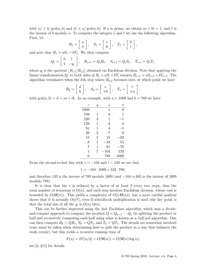
with |s| ≤ b/ gcd(a, b) and |t| ≤ a/ gcd(a, b). If a is prime, we obtain as + bt = 1, and t isthe inverse of b modulo a. To compute the integers s and t we use the following algorithm.First, let

R1 =

[ab

], S1 =

[10

], T1 =

[01

],

and note that R1 = aS1 + bT1. We then compute

Qi =

[0 11 −qi

], Ri+1 = QiRi, Si+1 = QiSi, Ti+i = QiTi,

where qi is the quotient bRi,1/Ri,2c obtained via Euclidean division. Note that applying thelinear transformation Qi to both sides of Ri = aSi+ bTi ensures Ri+1 = aSi+1+ bTi+1. Thealgorithm terminates when the kth step where Rk,2 becomes zero, at which point we have

Rk =

[d0

], Sk =

[s±b

], Tk =

[t∓a

],

with gcd(a, b) = d = sa+ tb. As an example, with a = 1009 and b = 789 we have

r q s t

1009 1 0789 1 0 1220 3 1 −1129 1 −3 491 1 4 −538 2 −7 915 2 18 −238 1 −43 557 1 61 −781 7 −104 1330 789 −1009

From the second-to-last line with s = −104 and t = 133 we see that

1 = −104 · 1009 + 133 · 789,

and therefore 133 is the inverse of 789 modulo 1009 (and −104 ≡ 685 is the inverse of 1009modulo 789).

It is clear that the r is reduced by a factor of at least 2 every two steps, thus thetotal number of iterations is O(n), and each step involves Euclidean division, whose cost isbounded by O(M(n)). This yields a complexity of O(nM(n)), but a more careful analysisshows that it is actually O(n2), even if schoolbook multiplication is used (the key point isthat the total size of all the qi is O(n) bits).

This can be further improved using the fast Euclidean algorithm, which uses a divide-and-conquer approach to compute the product Q = Qk−1 · · ·Q1 by splitting the product inhalf and recursively computing each half using what is known as a half-gcd algorithm. Onecan then compute Rk = QR1, Sk = QS1, and Tk = QT1. The details are somewhat involved(care must be taken when determining how to split the product in a way that balances thework evenly), but this yields a recursive running time of

T (n) = 2T (n/2) +O(M(n)) = O(M(n) log n);

see [3, §11] for details.

18.783 Spring 2019, Lecture #4, Page 4

Theorem 4.8. Let p be a prime. The time to invert an element of F×p is O(M(n) log n),where n = lg p.

The extended Euclidean algorithm works in any Euclidean ring, that is, a ring with anorm function that allows us to use Euclidean division to write a = qb + r with r of normstrictly less than b (for any nonzero b). This includes polynomial rings, in which the norm ofa polynomial is simply its degree. Thus we can compute the inverse of a polynomial moduloanother polynomial, provided the two polynomials are relatively prime.

One issue that arises when working in Euclidean rings other than Z is that there maybe units (invertible elements) other than ±1, and the gcd is only defined up to a unit.In the case of the polynomial ring Fp[x], every element of F×p is a unit, and with the fastEuclidean algorithm in Fp[x] one typically normalizes the intermediate results by making thepolynomials monic at each step; this involves computing the inverse of the leading coefficientin Fp. If Fq = Fp[x]/(f) with deg f = d, one can then bound the time to compute an inversein Fq by O(M(d) log d), operations in Fp, of which O(d) are inversions; see [3, Thm. 11.10(i)].This gives a bit complexity of

O(M(d)M(log p) log d+ dM(log p) log log p),

but with Kronecker substitution we can sharpen this to

O(M(d(log p+ log d)) log d+ dM(log p) log log p).

We will typically assume that either log d = O(log p) (large characteristic) or log p = O(1)(small characteristic); in both cases we can simplify this bound to O(M(n) log n), wheren = lg q = d lg p is the number of bits in q, the same result we obtained for the case whereq = p is prime.

Theorem 4.9. Let q = pd be a prime power and assume that either log d = O(log p) orp = O(1). The time to invert an element of F×q is O(M(n) log n), where n = lg q.

4.3 Exponentiation (scalar multiplication)

Let a be a positive integer. In a multiplicative group, the computation

ga = gg · · · g︸ ︷︷ ︸a

is known as exponentiation. In an additive group, this is equivalent to

ag = g + g + · · ·+ g︸ ︷︷ ︸a

,

and is called scalar multiplication. The same algorithms are used in both cases, and mostof these algorithms were first developed in a multiplicative setting (the multiplicative groupof a finite field) and are called exponentiation algorithms. It is actually more convenient todescribe the algorithms using additive notation (fewer superscripts), so we will do so.

The oldest and most commonly used exponentiation algorithm is the “double-and-add"method, also known as left-to-right binary exponentiation. Given an element P of an additivegroup and a positive integer a with binary representation a =

∑2iai, we compute the scalar

multiple Q = aP as follows:

18.783 Spring 2019, Lecture #4, Page 5

def DoubleAndAdd (P,a):a=a.digits(2); n=len(a) # represent a in binary using n bitsQ=P; # start 1 bit below the high bitfor i in range(n-2,-1,-1): # for i from n-2 down to 0

Q += Q # doubleif a[i]==1: Q += P # add

return Q

Alternatively, we may use the “add-and-double" method, also known as right-to-leftbinary exponentiation.

def AddAndDouble (P,a):a=a.digits(2); n=len(a) # represent a in binary using n bitsQ=0; R=P; # start with the low bitfor i in range(n-1):

if a[i]==1: Q += R # addR += R # double

Q += R # last addreturn Q

The number of group operations required is effectively the same for both algorithms. Ifwe ignore the first addition in the add_and_double algorithm (which could be replacedby an assignment, since initially Q = 0), both algorithms use precisely

n+wt(a)− 2 ≤ 2n− 2 = O(n)

group operations, where wt(a) = #{ai : ai = 1} is the Hamming weight of a, the number of1’s in its binary representation. Up to the constant factor 2, this is asymptotically optimal,and it implies that exponentiation in a finite field Fq has complexity O(nM(n)) with n = lg q;this assumes the exponent is less than q, but note that we can always reduce the exponentmodulo q − 1, the order of the cyclic group F×q . Provided the bit-size of the exponentis O(n2), the O(M(n2)) time to reduce the exponent modulo q− 1 will be majorized by theO(nM(n)) time to perform the exponentiation.

Notwithstanding the fact that the simple double-and-add algorithm is within a factorof 2 of the best possible, researchers have gone to great lengths to eliminate this factor of 2,and to take advantage of situations where either the base or the exponent is fixed, and thereare a wide variety of optimizations that are used in practice; see [2, Ch. 9] and [4]. Here wegive just one example, windowed exponentiation, which is able to reduce the constant factorfrom 2 to an essentially optimal 1 + o(1).

4.3.1 Fixed-window exponentiation

Let the positive integer s be a window size and write a as

a =∑

ai2si, (0 ≤ ai < 2s).

This is equivalent to writing a in base 2s. With fixed-window exponentiation, one firstprecomputes multiples dP for each of the “digits" d ∈ [0, 2s − 1] that may appear in thebase-2s expansion of a. One then uses a left-to-right approach as in the double-and-addalgorithm, except now we double s times and add the appropriate multiple aiP .

def FixedWindow (P,a,s):a=a.digits(2^s); n=len(a) # write a in base 2^s

18.783 Spring 2019, Lecture #4, Page 6

R = [0*P,P]for i in range(2,2^s): R.append(R[-1]+P) # precompute digitsQ = R[a[-1]] # copy the top digitfor i in range(n-2,-1,-1):

for j in range(0,s): Q += Q # double s timesQ += R[a[i]] # add the next digit

return Q

In the algorithm above we precompute multiples of P for every possible digit that mightoccur. As an optimization one could examine the base-2s representation of a and onlyprecompute the multiples of P that are actually needed.

Let n be the number of bits in a and let m = dn/se be the number of base-2s digits ai.The precomputation step uses 2s− 2 additions (we get 0P and 1P for free), there are m− 1additions of multiples of P corresponding to digits ai (when ai = 0 these cost nothing), andthere are a total of (m− 1)s doublings. This yields an upper bound of

2s − 2 +m− 1 + (m− 1)s ≈ 2s + n/s+ n

group operations. If we choose s = lg n− lg lgn, we obtain the bound

n/ lg n+ n/(lg n− lg lgn) + n = n+O(n/ log n),

which is (1 + o(1))n group operations.

4.3.2 Sliding-window exponentiation

The sliding-window algorithm modifies the fixed-window algorithm by “sliding" over blocksof 0s in the binary representation of a. There is still a window size s, but a is no longertreated as an integer written in a fixed base 2s. Instead, the algorithm scans the bits of theexponent from left to right, assembling “digits" of at most s bits with both high and lowbits set: with a sliding window of size 3 the bit-string 110011010101100 could be brokenup as 11|00|11|0|101|0|11|00 with 4 nonzero digits, whereas a fixed window approach woulduse 110|011|010|101|100 with 5 nonzero digits. This improves the fixed-window approachin two ways: first, it is only necessarily to precompute odd digits, and second, dependingon the pattern of bits in a, sliding over the zeros may reduce the number of digits used, asin the example above. In any case, the sliding-window approach is never worse than thefixed-window approach, and for s > 2 it is always better.

Example 4.10. Let a = 26284 corresponding to the bit-string 110011010101100 above. Tocompute aP using a sliding window approach with s = 3 one would first compute 2P, 3P, 5Pusing 3 additions and then

aP = 22 · (23 · (24 · (24 · (3P ) + 3P )) + 5P ) + 3P )

using 3 additions and 13 doublings, for a total cost of 19 group operations. A fixed windowapproach with s = 3 would instead compute 2P, 3P, 4P, 5P, 6P using 5 additions and

aP = 23 · (23 · (23 · (23 · 6P + 3P ) + 2P ) + 5P ) + 4P

using 4 additions and 12 doublings for a total cost of 21 group operations. Note that inboth cases we avoided computing 7P since it was not needed.

18.783 Spring 2019, Lecture #4, Page 7

4.4 Root-finding in finite fields

Let f(x) be a polynomial in Fq[x] of degree d. We wish to find a solution to f(x) = 0 thatlies in Fq. As an important special case, this will allow us to compute square roots usingf(x) = x2 − a, and, more generally, rth roots.2

The algorithm we give here was originally proposed by Berlekamp for prime fields [1], andthen refined and extended by Rabin [6], whose presentation we follow here. The algorithmis probabilistic, and is one of the best examples of how randomness can be exploited in anumber-theoretic setting. As we will see, it is quite efficient, with an expected running timethat is quasi-quadratic in the size of the input. By contrast, no deterministic polynomial-time algorithm for root-finding is known, not even for computing square roots.3

4.4.1 Randomized algorithms

Probabilistic algorithms are typically classified as one of two types: Monte Carlo or LasVegas. Monte Carlo algorithms are randomized algorithms whose output may be incorrect,depending on random choices that are made, but whose running time is bounded by afunction of its input size, independent of any random choices. The probability of error isrequired to be less than 1/2−ε, for some ε > 0, and can be made arbitrarily small be runningthe algorithm repeatedly and using the output that occurs most often. In contrast, a LasVegas algorithm always produces a correct output, but its running time may depend onrandom choices; we do require that its expected running time is finite. As a trivial example,consider an algorithm to compute a+ b that first flips a coin repeatedly until it gets a headand then computes a + b and outputs the result. The running time of this algorithm maybe arbitrarily long, even when computing 1 + 1 = 2, but its expected running time is O(n),where n is the size of the inputs.

Las Vegas algorithms are generally preferred, particularly in mathematical applications.Note that any Monte Carlo algorithm whose output can be verified can always be convertedto a Las Vegas algorithm (just run the algorithm repeatedly until you get an answer that isverifiably correct). The root-finding algorithm we present here is a Las Vegas algorithm.

4.4.2 Using GCDs to find roots

Recall from the previous lecture that we defined the finite field Fq to be the splitting fieldof xq − x over its prime field Fp; this definition also applies when q = p is prime (sincexp− x splits completely in Fp), and in every case, the elements of Fq are precisely the rootsof xq − x. The roots of f that lie in Fq are the roots it has in common with the polynomialxq − x. We thus have

g(x) := gcd(f(x), xq − x) =∏i

(x− αi),

where the αi range over all the distinct roots of f that lie in Fq. If f has no roots in Fq theng will have degree 0 (in which case g = 1). We have thus reduced our problem to finding aroot of g, where g has distinct roots that are known to lie in Fq.

2An entirely different approach to computing rth roots using discrete logarithms is explored in ProblemSet 2. It has better constant factors when the r-power torsion subgroup of F∗

q is small (which is usually thecase), but is asymptotically slower then the algorithm presented here in the worst case.

3Deterministic polynomial-time bounds for root-finding can be proved in various special cases, includingthe computation of square-roots, if one assumes a generalization of the Riemann hypothesis.

18.783 Spring 2019, Lecture #4, Page 8

In order to compute g = gcd(f, xq − x) efficiently, we generally do not compute xq − xand then take the gcd with f ; this would take time exponential in n = log q.4 Instead, wecompute xq mod f by exponentiating the polynomial x to the qth power in the ring Fq[x]/(f),whose elements are uniquely represented by polynomials of degree less than d = deg f . Eachmultiplication in this ring involves the computation of a product in Fq[x] followed by areduction modulo f ; note that we do not assume Fq[x]/(f) is a field (indeed for deg f > 1,if f has a root in Fq then Fq[x]/(f) is definitely not a field). This reduction is achievedusing Euclidean division, and can be accomplished using two polynomial multiplicationsonce an approximation to 1/f has been precomputed, see §4.1, and is within a constantfactor of the time to multiply two polynomials of degree d in any case. The total cost ofeach multiplication in Fq[x]/(f) is thus O(M(d(n+log d))), assuming that we use Kroneckersubstitution to multiply polynomials. The time to compute xq mod f using any of theexponentiation algorithms described in §4.3 is then O(nM(d(n+ log d))).

Once we have computed xq mod f , we subtract x and compute g = gcd(f, xq−x). Usingthe fast Euclidean algorithm, this takes O(M(d(n+ log d)) log d) time. Thus the total timeto compute g is O(M(d(n + log d))(n + log d)); and in the typical case where log d = O(n)(e.g. d is fixed and only n is growing) this simplifies to O(nM(dn)).

So far we have not used randomness; we have a deterministic algorithm to compute thepolynomial g = (x− r1) · · · (x− rk), where r1, . . . , rk are the distinct Fq-rational roots of f .We can thus determine the number of distinct roots f has (this is just the degree of g), andin particular, whether it has any roots, deterministically, but knowledge of g does not implyknowledge of the roots r1, . . . , rk when k > 1; for example, if f(x) = x2 − a has a nonzerosquare root r ∈ Fq, then g(x) = (x− r)(x+ r) = f(x) tells us nothing beyond the fact thatf(x) has a root.

4.5 Randomized GCD splitting

Having computed g, we seek to factor it into two polynomials of lower degree by againapplying a gcd, with the goal of eventually obtaining a linear factor, which will yield a root.

Assuming that q is odd (which we do), we may factor the polynomial xq − x as

xq − x = x(xs − 1)(xs + 1),

where s = (q − 1)/2. Ignoring the root 0 (which we can easily check separately), thisfactorization splits F×q precisely in half: the roots of xs − 1 are the elements of F×q that aresquares in F×q , and the roots of xs + 1 are the elements of F×q that are not. Recall that F×qis a cyclic group of order q − 1, which is even (since q is odd), thus the squares in F×q arethe elements that are even powers of a generator, equivalently, elements whose order divides(q − 1)/2. If we compute

h(x) = gcd(g(x), xs − 1),

we obtain a divisor of g whose roots are precisely the roots of g that are squares in F×q . If wesuppose that the roots of g are as likely to be squares as not, we should expect the degreeof h to be approximately half the degree of g. And so long as the degree of h is strictlybetween 0 and deg g, one of h or g/h is a polynomial of degree at most half the degree of g,whose roots are all roots of our original polynomial f .

4The exception is when d > q, but in this case computing gcd(f(x), xq − x) takes O(M(d(n+ log d) log d)time, which turns out to be the same bound that we get for computing xq mod f(x) in any case.

18.783 Spring 2019, Lecture #4, Page 9

To make further progress, and to obtain an algorithm that is guaranteed to work nomatter how the roots of g are distributed in Fq, we take a probabilistic approach. Ratherthan using the fixed polynomial xs − 1, we consider random polynomials of the form

(x+ δ)s − 1,

where δ is uniformly distributed over Fq. We claim that if α and β are any two nonzeroroots of g, then with probability 1/2, exactly one of these is a root (x+ δ)s − 1. It followsfrom this claim that so long as g has at least 2 distinct nonzero roots, the probability thatthe polynomial h(x) = gcd(g(x), (x+ δ)s + 1) is a proper divisor of g is at least 1/2.

Let us say that two elements α, β ∈ Fq are of different type if they are both nonzero andαs 6= βs. Our claim is an immediate consequence of the following theorem from [6].

Theorem 4.11 (Rabin). For every pair of distinct α, β ∈ Fq we have

#{δ ∈ Fq : α+ δ and β + δ are of different type} = q − 1

2.

Proof. Consider the map φ(δ) = α+δβ+δ , defined for δ 6= −β. We claim that φ is a bijection

form the set Fq − {−β} to the set Fq − {1}. The sets are the same size, so we just need toshow surjectivity. Let γ ∈ Fq − {1}, then we wish to find a solution σ 6= −β to γ = α+σ

β+σ .We have γ(β + σ) = α + σ which means σ − γσ = γβ − α. This yields σ = γβ−α

1−γ ; we haveγ 6= 1, and σ 6= −β, because α 6= β. Thus φ is surjective.

We now note thatφ(δ)s =

(α+ δ)s

(β + δ)s

is −1 if and only if α+ δ and β + δ are of different type. The elements γ = φ(δ) for whichγs = −1 are precisely the non-residues in Fq\{1}, of which there are exactly (q − 1)/2.

We now give the algorithm, which assumes that its input f ∈ Fq[x] is monic (has leadingcoefficient 1). If f is not monic we can make it so by dividing f by its leading coefficient,which does not change its roots (or the complexity of computing them).

Algorithm 4.12. Given a monic polynomial f ∈ Fq[x], output an element r ∈ Fq such thatf(r) = 0, or null if no such r exists.

1. If f(0) = 0 then return 0.2. Compute g = gcd(f, xq − x).3. If deg g = 0 then return null.4. While deg g > 1:

a. Pick a random δ ∈ Fq.b. Compute h = gcd(g, (x+ δ)s − 1).c. If 0 < deg h < deg g then replace g by h or g/h, whichever has lower degree.

5. Return r, where g(x) = x− r.

It is clear that the output of the algorithm is always correct: either it outputs a rootof f in step 1, proves that f has no roots in Fq and outputs null in step 3, or outputs aroot of g that is also a root of f in step 5 (note that whenever g is updated it replaced witha proper divisor). We now consider its complexity.

18.783 Spring 2019, Lecture #4, Page 10

4.5.1 Complexity analysis

It follows from Theorem 4.11 that the polynomial h computed in step 4b is a proper divisorof g with probability at least 1/2, since g has at least two distinct nonzero roots α, β ∈ Fq.Thus the expected number of iterations needed to obtain a proper factor h of g is boundedby 2, and the expected cost of obtaining such an h is O(M(e(n + log e))(n + log e)), wheren = log q and e = deg g, and this dominates the cost of the division in step 4c.

Each time g is updated in step 4c its degree is reduced by at least a factor of 2. It followsthat the expected total cost of step 4 is within a constant factor of the expected time tocompute the initial value of g = gcd(f, xq−x), which is O(M(d(n+log d))(n+log d)), whered = deg f ; this simplifies to O(nM(dn)) in the typical case that log d = O(n), which holdsin all the applications we shall be interested in.

4.5.2 Finding all roots

Wemodify our algorithm to find all the distinct roots of f , by modifying step 4c to recursivelyfind the roots of both h and g/h. In this case the amount of work done at each level ofthe recursion tree is bounded by O(M(d(n+ log d))(n+ log d)). Bounding the depth of therecursion is somewhat more involved, but one can show that with very high probability thedegrees of h and g/h are approximately equal and that the expected depth of the recursionis O(log d). Thus we can find all the distinct roots of f in

O(M(d(n+ log d))(n+ log d) log d)

expected time. When log d = O(n) this simplifies to O(nM(dn) log d).Once we know the distinct roots of f we can determine their multiplicity by repeated

division, but this is not the most efficient approach. By taking GCDs with derivatives one canfirst compute the squarefree factorization of f , which for a monic nonconstant polynomial fis defined as the unique sequence g1, . . . , gm ∈ Fq[x] of monic squarefree coprime polynomialswith gm 6= 1 such that

f = g1g22g

33 · · · gmm.

This can be done using Yun’s algorithm [7] (see Algorithm 14.21 and Exercise 14.30 in [3])using O(M(d) log d) operations in Fq, which is dominated by the complexity bound for root-finding determined above. The cost of finding the roots of all the gi is no greater than thecost of finding the roots of f (the complexity of root-finding is superlinear in the degree),and with this approach we know a priori the multiplicity of each root as a root of f . Itfollows that we can determine all the roots of f and their multiplicities, within the timebound given above for finding the distinct roots of f .

4.6 Computing a complete factorization

Factoring a polynomial f ∈ Fq[x] into irreducibles can effectively be reduced to finding rootsof f in extensions of Fq. Linear factors of f correspond to the roots of f in Fq, irreduciblequadratic factors of f correspond to roots of f that lie in Fq2 but do not lie in Fq; recall fromCorollary 3.9 that every quadratic polynomial Fq[x] splits completely in Fq2 [x]. Similarly,each irreducible degree d-factor of f corresponds to a root of f that lies in Fqd but none ofits proper subfields.

We now sketch the algorithm; see [3, §14] for further details on each step.

18.783 Spring 2019, Lecture #4, Page 11

Algorithm 4.13. Given a monic polynomial f ∈ Fq[x], compute its irreducible factorizationin Fq[x] as follows:

1. Determine the largest power xe dividing f and replace f with f/xe.2. Compute the squarefree factorization f = g1g

22 · · · gmm of f using Yun’s algorithm.

3. By successively computing gij = gcd(gi, xqj − x) and replacing gi with gi/gij for

j = 1, 2, 3, . . . .deg gi, factor each gi into polynomials gij that are each (possibly trivial)products of distinct irreducible polynomials of degree j; note that once j > (deg gi)/2we know gi must be irreducible and can immediately determine all the remaining gij .

4. Factor each nontrivial gij into irreducible polynomials hijk of degree j as follows:while deg gij > j generate random monic polynomials u ∈ Fq[x] of degree j untilh := gcd(gij , u

(qj−1)/2 − 1) properly divides gij , then recursively factor h and gij/h.5. Output x with multiplicity e and output each gijk with multiplicity i.

In step 3, for j > 1 one computes hj := xqjmod gij via hj = hqj−1 mod qij . The expected

cost of computing the gij for a given gi of degree d is then bounded by

O(M(d(n+ log d))d(n+ log d)),

which simplifies to O(dnM(dn)) when log d = O(n) and is in any case quasi-quadratic inboth d and n. The cost of factoring a particular gij satisfies the same bound with d replacedby j; the fact that this bound is superlinear and deg gi =

∑j deg gij implies that the cost

of factoring all the gij for a particular gi is bounded by the cost of computing them, andsuperlinearity also implies that simply putting d = deg f gives us a bound on the cost ofcomputing the gij for all the gi, and this bound also dominates the O(M(d)(log d)M(n))complexity of step 1.

As a special case, Algorithm 4.13 can be used as a deterministic algorithm for irreducibil-ity testing; steps 1-3 do not involve any random choices and suffice to determine whether ornot the input is irreducible (this holds if and only if g1d is the only nontrivial gij).

There are faster algorithms for polynomial factorization (including algorithms that aresub-quadratic in the degree) that use linear algebra in Fq; see [3, 14.8]. These are of interestprimarily when the degree d is large relative to n = log q or the characteristic is small.

4.6.1 Summary

The table below summarizes the bit-complexity of the various arithmetic operations wehave considered, both in the integer ring Z and in a finite field Fq of characteristic p withq = pe, where we assume either log e = O(log q) (large characteristic) or p = O(1) (smallcharacteristic); in both cases n is the bit-size of the inputs (so n = log q for Fq).

integers Z finite field Fqaddition/subtraction O(n) O(n)multiplication M(n) O(M(n))Euclidean division (reduction) O(M(n)) O(M(n))extended gcd (inversion) O(M(n) log n) O(M(n) log n)exponentiation O(nM(n))square-roots (probabilistic) O(nM(n))root-finding (probabilistic) O(M(d(n+ log d))(n+ log d))factoring (probabilistic) O(M(d(n+ log d))d(n+ log d))irreducibility testing O(M(d(n+ log d))d(n+ log d))

18.783 Spring 2019, Lecture #4, Page 12

In the case of root-finding, factorization, and irreducibility testing, d is the degree of thepolynomial, and for probabilistic algorithms these are bounds on the expected running timeof a Las Vegas algorithm. The bound for exponentiation assumes that the bit-length of theexponent is O(n2).

References

[1] Elwyn R. Berlekamp, Factoring polynomials over large finite fields, Mathematics of Com-putation 24 (1970), 713–735.

[2] Henri Cohen et al., Handbook of elliptic and hyperelliptic curve cryptography , CRC Press,2006.

[3] Joachim von zur Gathen and Jürgen Gerhard, Modern computer algebra, third edition,Cambridge University Press, 2013.

[4] Daniel M. Gordon, A survey of fast exponentiation methods, Journal of Algorithms 27(1998), 129–146.

[5] David Harvey, Joris van der Hoeven, and Grégoire Lecerf, Faster polynomial multiplica-tion over finite fields, Journal of the ACM 63 (2017), Art. 52, 23 pages.

[6] Michael O. Rabin, Probabilistic algorithms in finite fields, SIAM Journal of Computing 9(1980), 273–280.

[7] David Y.Y. Yun, On square-free decomposition algorithms, in Proceedings of the thirdACM symposium on symbolic and algebraic computation (SYMSAC ‘76), R.D. Jenks(ed.), ACM Press, 1976, 26–35.

18.783 Spring 2019, Lecture #4, Page 13