IZA DP No. 120

Does Education Reduce Wage Inequality?Quantile Regressions Evidence fromFifteen European Countries

Pedro Telhado PereiraPedro Silva Martins

DI

SC

US

SI

ON

PA

PE

R S

ER

IE

S

Forschungsinstitutzur Zukunft der ArbeitInstitute for the Studyof Labor

February 2000

Does Education Reduce Wage Inequality? Quantile Regressions Evidence from

Fifteen European Countries

Pedro Telhado Pereira Universidade Nova de Lisboa, CEPR and IZA, Bonn

Pedro Silva Martins Universidade Nova de Lisboa

Discussion Paper No. 120 February 2000

IZA

P.O. Box 7240 D-53072 Bonn

Germany

Tel.: +49-228-3894-0 Fax: +49-228-3894-210

Email: iza@iza.org

This Discussion Paper is issued within the framework of IZA’s research areas The Future of Work and General Labor Economics. Any opinions expressed here are those of the author(s) and not those of the institute. Research disseminated by IZA may include views on policy, but the institute itself takes no institutional policy positions. The Institute for the Study of Labor (IZA) in Bonn is a local and virtual international research center and a place of communication between science, politics and business. IZA is an independent, nonprofit limited liability company (Gesellschaft mit beschränkter Haftung) supported by the Deutsche Post AG. The center is associated with the University of Bonn and offers a stimulating research environment through its research networks, research support, and visitors and doctoral programs. IZA engages in (i) original and internationally competitive research in all fields of labor economics, (ii) development of policy concepts, and (iii) dissemination of research results and concepts to the interested public. The current research program deals with (1) mobility and flexibility of labor markets, (2) internationalization of labor markets and European integration, (3) the welfare state and labor markets, (4) labor markets in transition, (5) the future of work, (6) project evaluation and (7) general labor economics. IZA Discussion Papers often represent preliminary work and are circulated to encourage discussion. Citation of such a paper should account for its provisional character.

IZA Discussion Paper No. 120 February 2000

ABSTRACT

Does Education Reduce Wage Inequality? Quantile Regressions Evidence from

Fifteen European Countries*

We address the impact of education upon wage inequality by drawing on evidence from fifteen European countries, during a period ranging between 1980 and 1995. We focus on within-educational-levels wage inequality by estimating quantile regressions of Mincer equations and analysing the differences in returns to education across the wage distribution and across time. Four different patterns emerge: 1) a positive and increasing contribution of education upon within-levels wage inequality –the case of Portugal; 2) a positive but stable role of education in terms of inequality – Austria, Finland, France, Ireland, Netherlands, Norway, Spain, Sweden, Switzerland, UK; 3) a neutral role – Denmark and Italy; and 4) a negative impact – Germany and Greece. We thus find that in most countries dispersion in earnings increases with educational levels and that education is a risky investment. These results suggest a positive interaction between schooling and ability with respect to earnings. JEL Classification: C29, D31, I21, J24, J31 Keywords: Returns to education, earnings inequality, quantile regressions, ability,

education systems, labour-market institutions Pedro Telhado Pereira Faculdade de Economia Universidade Nova de Lisboa Travessa Estêvão Pinto P-1099-032 Lisboa Portugal Email: ppereira@fe.unl.pt

* This paper was written under the scope of the 15-country ‘PuRE - Public Funding and Private Returns to Education’ European Commission TSER project. The results reported here that refer to countries other than Portugal were produced by the corresponding PuRE partners. For more information on this project and the member teams, please check www.etla.fi/PURE. We thank participants at the PuRE Paris and Barcelona seminarsand José Vieira for comments and suggestions. The usual disclaimer applies. P. T. Pereira: Research support granted by Banco de Portugal and Fundação para a Ciência e a Tecnologia is kindly acknowledged. P. S. Martins: Financial support from the European Commission TSER programme under contract SOE2-CT98-2044 is gratefully acknowledged.

2

Extended abstract:

Education has long been considered a multipurpose policy tool. A related belief is that increased

educational attainment will lead to less wage inequality. Consequently, given the current situation

of increasing inequality in most developed societies, of which globalisation is a much-cited

culprit, policy-makers have been very keen to demand further public funding for schooling.

However, it might be the case that such an approach proves ineffective. For instance, if education

systems are poorly designed, former students may not benefit financially –at the labour market–

from the qualifications they acquired at schools. Another possibility is that ability interacts

powerfully with schooling, which would imply that a more educated workforce would be

associated with more wage inequality.

In this paper, we study this topic –the link between education and inequality– which we find

crucial for Western societies. We start by putting forward three channels whereby education

impacts upon inequality: inter- and intra-educational-levels (between- and within-educational-

levels) earnings differentials and changes in the distribution of schooling.

We focus on within-educational-levels earnings differentials and suggest that quantile

regressions should be used for uncovering them. Quantile regressions allow for different impacts

of education along the whole conditional distribution of earnings, unlike the more common

Ordinary Least Squares estimates, which focus on mean returns.

In the empirical sections, we compare quantile regression results of returns to education based on

Mincer regressions from fifteen European countries (Austria, Denmark, France, Finland,

Germany, Greece, Italy, Ireland, Netherlands, Norway, Portugal, Spain, Sweden, Switzerland and

the United Kingdom). Each country is covered by approximately a 15-year time-span (between

1980 and 1995).

Four contrasting patterns emerge:

1) an increasingly positive role of education upon intra-educational-levels inequality, where

the best (worst) paid at each educational level reap higher (lower) benefits from education

and where such a best-worst differential has increased over time (Portugal);

2) a positive but stable relationship between education and within-levels inequality (Austria,

Finland, France, Ireland, Netherlands, Norway, Spain, Sweden, Switzerland and the UK);

3

3) a neutral impact of education upon within-levels inequality, as there are no sizeable

differences in returns to education across the wage distribution (Denmark and Italy); and

4) a negative relationship between returns to education and the wage distribution (Germany

and Greece).

These results, which provide a summary assessment of the outcome of the interaction between

education systems and labour-market institutions, suggest that, in most countries, the dispersion

in earnings increases with educational levels. This is the case in eleven out of fifteen countries,

whereas in two countries the dispersion of earnings proves stable across different educational

levels and in two others earnings are less dispersed for higher educational levels. Given this

evidence, and in the context of within-levels inequality, we conclude that education does not

reduce wage inequality.

Moreover, if we assume that such characteristics can be proxied by ability then our results say

that there is a positive interaction between ability and education: the higher the ability level, the

stronger will the impact of schooling be on one’s wages. This result supports ‘Bell curve’ type of

arguments which place much emphasis on the role of cognitive ability on economic and social

success.

These results also suggest that education is a risky investment. To the extent that prospective

students are unaware of the characteristics which will place them at some point along a wide

earnings distribution, the financial outcome of their education decision is largely unpredictable.

This situation might also correspond to over-education, in the sense that the marginal reward

some individuals reap from their schooling is very low or even negative. Such individuals will

thus not benefit financially from the costly investments they engage in. Standard OLS returns

thus disregard an enormous amount of variety in returns which is underlying the data from most

countries. This also implies that drawing on simple OLS returns for policy-making might prove

rather elusive and misleading.

In terms of policy-making, we believe that these overall results are useful as they amount to a

summary, ex-post characterisation of the joint functioning of each country’s national education

system and labour-market institutions. Should wage equality be considered as a policy goal, a

country where such a joint mechanism promotes inequality might wish to pinpoint and reverse

the underlying causes.

4

1. Introduction

Education has long been considered a multipurpose policy tool. One of the goals customarily

attached to education policy is that increased educational attainment will lead to less wage

inequality. Consequently, and given the current situation of increasing inequality in most

developed societies,3,4 policy-makers have been very keen to demand and support further public

funding for schooling activities.5

More importantly still, many see education as the only tool available for governments to reverse

or, at least, slow down the inequality-enhancing impact attributed to globalisation. In fact,

regardless of the explanation we choose for such impact of globalisation upon inequality –either

trade or technology6-, the element of skills is always crucial and must therefore be at the heart of

the rise in inequality witnessed in most developed countries.7

However, and contrary to this more common approach, one might also very well think of a

number of situations where increasing educational attainment will lead to higher, not lower,

earnings inequality. Two examples should suffice: 1) poorly designed or outdated education

systems, where students are provided with skills in large supply and little demand in the labour

market; and 2) elitist educational systems, where some schools which accept only a few

candidates (not necessarily the most talented) concentrate all the job-market signalling that

prospective employers are interested in.

More fundamentally, ability might play a more important role in terms of the worker’s

productivity (and pay) at higher educational levels. In fact, if there is a powerful interaction

3 See OECD (1995) and Table 1.1. It is very clear that the majority of the OECD countries covered have witnessedincreasing income inequality during the 1980’s. Although, there is no evidence on the evolution of inequality duringthe early 1990’s, for most countries we find no reasons to assume that this pattern has changed.4 There is a wealth of US-based literature on this issue: among others, see Lee (1999), Gottschalk (1997), Blau andKahn (1996), Juhn et al. (1993) and Katz and Murphy (1992). For Europe, see Leuven et al. (1997). A morecomprehensive and international work is Gottschalk and Smeeding (1997). Finally, a thorough and recent generalreference on inequality can be found in Champernowne and Cowell (1998).5 See the recent speech of the Portuguese minister of education at a UNESCO conference -Oliveira Martins (1999).6 Trade with less-developed countries in goods which are intensive in unskilled labour would, the argument goes,create a downward pressure on the earnings of the unskilled labour force of the developed countries. On the otherhand, technological progress would make those workers who are less able to interact with such new technologies lessappealing in the labour market. Consequently, their earnings would either fall or increase less than those of theskilled labour force.7 We follow the standard view of regarding inequality as bad. See Welch (1999) for a contrasting, non-mainstreamapproach.

5

between education and ability, the current process of rising educational attainment would lead,

per se, to further earnings dispersion.8 If ability interacts powerfully with schooling, a more

educated workforce would be associated with more wage inequality.

In this context of conflicting a priori evidence, we believe that it is of the utmost importance to

assess empirically the direction of the effective impact of education upon inequality. If education

proves to be, after all, a less appealing policy tool in terms of reducing inequality, then the huge

investments currently being made should be placed under scrutiny. It might very well be the case

that alternative applications of public funds are more effective for placing each society at its

preferred situation in terms of the efficiency-equity trade-off boundaries.9

Moreover, given the very diverse situation across European countries in terms of both their

educational and labour-market institutions –which are those most likely to shape the wage

distribution and, thus, wage inequality– one could expect that such a link between education and

inequality would adopt different patterns. This aspect could prove rather insightful and

informative in the sense that it would suggest different country models to be followed according

to the goals in mind.

Given this background, we draw on quantile regression results of Mincer equations from fifteen

European countries in order to address the link between education and inequality. Quantile

regressions are a technique that allows one to differentiate the contribution of regressors along the

distribution of the endogenous variable and not simply at the mean, as with OLS.

We use this feature to assess any differences in terms of the rewards to education for individuals

from different portions of the wage distribution and thus conclude on the link between education

and inequality. Simultaneously, we provide evidence to answer Card’s (1994) question ‘Is the

labour force reasonably well-described by a constant return to education for all workers?’ [page

33, author’s italics].

8 See OECD (1997) for a survey of recent developments in schooling attainment.9 See Heckman (1999) for a very insightful analysis and evaluation of policy experiments in education in the UnitedStates and also an example of the need to assess the effectiveness of education policies. This author suggests that adislocation of investment from upper to lower educational levels is in need. He argues that as ‘learning begetslearnings’, improving the access and quality of education at early ages will have a strong effect on the individual’slife-long prospects.

6

Our paper goes as follows: in Section 2, a brief presentation of the econometric theory behind

quantile regressions is offered. In Section 3, we explain how we use such results to draw

conclusions in terms of the (different) impact education might have upon inequality across

Europe. Section 4 presents the data-sets used in each country, together with some descriptive

statistics. In the following section we compare the differences that emerge among the countries

surveyed in terms of returns to years of education. Finally, Section 6 presents a brief summary of

the paper and concludes.

2. Quantile regressions

‘“On the average” has never been a satisfactory statement with which toconclude a study on heterogeneous populations. Characterisation of theconditional mean constitutes only a limited aspect of possibly moreextensive changes involving the entire distribution.’

Buchinsky (1994, page 453)10

An ordinary least squares (OLS) regression is based on the mean of the conditional distribution of

the regression’s dependent variable. This approach is used because one implicitly assumes that

possible differences in terms of the impact of the exogenous variables along the conditional

distribution are unimportant.

However, this may prove inadequate in some research agendas. If exogenous variables influence

parameters of the conditional distribution of the dependent variable other than the mean, then an

analysis which disregards this possibility will be severely weakened (see Koenker and Bassett,

1978). Unlike OLS, quantile regression models allow for a full characterisation of the conditional

distribution of the dependent variable.11,12

10 An alternative quote might be taken from Mosteler and Tukey, 1977, p. 266, quoted in Mata and Machado (1996):“What the regression curve does is give a grand summary for the averages of the distributions corresponding to theset of x’s. […] Just as the mean gives an incomplete picture of a single distribution, so the regression curve gives acorrespondingly incomplete picture for a set of distributions”.11 If the dependent variable is distributed identically around a known function of the regressors, then the distributionof y given x is a translation family. If one ‘connects’ the different averages of the conditional distribution fordifferent values of x, one gets the mean or OLS regression. One might also connect the points associated withdifferent quantiles of the distribution of y given x for different values of x, thus getting regression quantiles, and allthese regressions would be parallel. The information about the impact of different regressors on different measures oflocalisation would then be the same. However, in most cases, the distribution of y given x is not a translation family.In these cases, different regressions provide different results concerning the way y varies with x. Quantile regressionsallow for this to be done, as they may characterise the entire conditional distribution of the dependent variable. It isusually the case that there are information gains from estimating more regressions than simply the mean regression.

7

The quantile regression model can be written as (see Buchinsky (1994)):

(1) θθθθ ββ iiiiii xxwuxw =+= )(lnQuantwithln

where ix is the vector of exogenous variables and θβ is the vector of parameters. )(lnQuant xwθ

denotes the θ th conditional quantile of wln given x . The θ th regression quantile, 10 <<θ , is

defined as a solution to the problem:

(2) .ln)1(lnmin::

−−+− ∑∑<≥∈ β

θβ

θβ

βθβθiiii

kxyi

iixyi

iiR

xwxw

This is normally written as:

(3) ∑ −∈ i

iiR

xwk

)(lnmin θθβ

βρ ,

where )(ερθ is the check function defined as θεερθ =)( if 0≥ε or εθερθ )1()( −= if

0<ε .13

This problem does not have an explicit form but can be solved by linear programming methods.

Standard errors are obtainable by bootstrap methods.

The least absolute deviation (LAD) estimator of β is a particular case within this framework. This

is obtained by setting θ=0.5 (the median regression). The first quartile is obtained by setting

θ=0.25 and so on. As one increases θ from 0 to 1, one traces the entire distribution of y,

conditional on x.

We provide a simple example of the usefulness of quantile regressions by considering gender

wage differentials in Portugal. We draw on a 1995 sample from Quadros de Pessoal, a rich

12 See Abadie et al (1999) for a recent extension of quantile regressions, considering instrumental variables.13 This procedure is basically an extension of the method used for computing simple quantiles of a distribution.

8

employer-based data-set14 and run a simple OLS regression of log hourly earnings on a constant

and a dummy, taking value one for women and value zero for men:

(4) iii ufemalehw ++= .)/ln( βα

In this very simple setting, the coefficient associated with this dummy variable can be interpreted

as the average pay differential between men and women. Our result (see last row of Table 2.2)

indicates that such a differential is -0.27.

However, should one analyse the distributions of earnings for men and women, one realises that

the shape of the distributions is very different (see Graph 2.1). For instance, we notice (see Table

2.1) that women’s hourly wages peak at the 5.84 and 5.88 classes, with a 5.7% frequency, while

the corresponding class for men is 6.2, with only a 4.1% frequency. In Table 2.2 we realise that

the gender difference in earnings increases substantially as one moves upward in the deciles of

each distribution. While the difference of average hourly wages for the lower 10% of each

distribution is –0.058, this figure increases to –0.288 at the fifth class, reaching –0.323 for the last

income class.

This succinct analysis shows very clearly that gender differences in earnings go well beyond the

fact that men, on average, earn more than women. However, should one consider this issue by

simply drawing on OLS estimates, much information contained in the data would be lost. We run

an OLS regression for our data and obtained a coefficient of –0.27.

Quantile regressions, on the other hand, enable one to better understand how the two distributions

differ. Effectively, the same dummy coefficient, when resulting from this latter type of

regression, mimics the differences in pay at different points of the wage distribution. It increases

from –0.099 for the first decile, increasing to –0.3 at the median and –0.315 at the top decile.

Summing up, quantile regressions provide snap-shots of different points of a conditional

distribution. They therefore constitute a parsimonious way of describing the whole distribution

and should bring much value-added if the relationship between the regressors and the

independent variable evolves across its conditional distribution. Given the discussion in Section

14 All firms operating in Portugal are required to fill in a table with extensive information on each worker and on thefirm itself. This requirement has been in force since the early 1980’s, thus providing an excellent source of

9

1, namely the suggestion that education might be impacting very differently across the wage

distribution, we employ this methodology for the education-earnings relationship.15,16

3. Decomposing education-related inequality

We consider three channels through which education might influence wage inequality: within-

and between-levels inequality and changes in the schooling distribution. The first channel is due

to the differences in mean earnings associated with individuals having different educational

levels. Such differences are deeply related to OLS returns to education.

The second channel, within-levels, inequality, has to do with the different degree of dispersion of

earnings at each educational level. This channel is better depicted by quantile regressions as we

will show below. This is also the link upon which we focus throughout the paper.

Finally, changes in the distribution of schooling should also be acknowledged as a link between

education and inequality. If the labour force is getting more educated (due either to life-long

training or, more importantly, to the increasing educational attainment of new cohorts) then the

overall level of inequality should also be affected.

Bearing this framework in mind, we distinguish between three possible situations concerning the

impact of education upon inequality. These three cases concern only within-levels inequality. In a

first situation we consider equal returns across the wage distribution. This would mean that such

distributions are identical for all educational levels.

The only difference lies in their position, as they get shifted further to the right (higher mean

wages) as the educational level is higher. In this case, education could not be associated with

information for labour-market oriented research. See Section 4 for more information on this dataset.15 This methodology proved fruitful in previous similar analyses, namely Machado and Mata (1998) and Hartog et al.(1999) –for Portugal–, Fersterer and Winter-Ebmer (1999) –for Austria– and Garcia et al. (1997) –for Spain.16 We assume throughout the paper that the nature of the link between schooling and earnings is a causal one. Whiletheoretically one might certainly point out that schooling is not an exogenous regressor in Mincer equations,empirical results suggest that the extent of the bias in education coefficients is small –see Card (1999). See also theLocal Average Treatment Effect (LATE) literature (Imbens and Angrist (1994) and Ichino and Winter-Ebmer(1999)) for a more careful analysis of causality in economic events in general and the education-earnings relationshipin particular.

10

within-levels inequality given that the dispersion of the different conditional wage distributions is

always the same.

A second case occurs when returns to education increase as one moves upward in the wage

distribution. As the next section will show, this is the most common case across our sample of

European countries. This would mean that wage distributions which depend on progressively

higher educational levels are more disperse.17 Here, schooling would have a positive impact upon

wage inequality.

Thirdly, the final possible case is that returns to education fall as one considers higher quantiles.

Unlike the situations before, intra-education inequality would decrease (as wage distributions

conditional on higher educational levels are less disperse).

In a nutshell, our procedure for linking education with earnings inequality involves decomposing

the contribution of the first upon the second into three effects: intra-education and inter-education

inequality and the distribution changes. The first refers to the progression of the dispersion of

conditional distributions of earnings: for instance, if such distributions ‘shrink’, then this

component’s contribution is negative (i.e. decreases inequality).

The second effect refers to the extent of the rightward shifts in such distributions as we move

upward in the educational levels. This is closely associated with the size of returns to education.

Finally, the third effect deals with changes in the educational attainment of the labour force.

As the second effect should always be positive (because returns to education have always been

positive so far), the first effect, intra-education inequality (which is associated with the slope of

the returns-deciles relationship as derived from regression quantiles) either reinforces or weakens

(and eventually reverses) the second effect. If one disregards the third effect, an asymmetry

would arise: while a positively-sloped returns-deciles relationship is a sufficient condition for

concluding that education contributes positively to inequality, a negatively-sloped curve is only a

necessary condition for concluding that education contributes negatively to inequality.

17 In econometric terms, this would be interpreted as evidence of heteroskedasticity. In fact, quantile regressions arealso used for tests of such non-spherical disturbances (see Koenker and Bassett (1982)).

11

Throughout the remaining chapters we will focus on the returns-deciles relationship drawing on

data from fifteen European countries.

4. Data-sets description

The results for each country were derived from a specific data-set used by each country’s team.

Table 4.1 describes such data-sets, including a short characterisation of its nature, the years

covered, the number of observations used for each year and also a reference on the procedure

adopted for dropping outlier observations.

Most data-sets are household surveys. Some countries have used labour-market oriented surveys

(Denmark, France and Switzerland) and an employer-based data-set (Portugal). The number of

observations used varies a great deal, ranging from fewer than 2,000 (Finland, Norway and

Sweden) to more than 25,000 (Portugal and Spain –for 1995).

There is also some variation in terms of the procedure for dealing with potential outliers. Some

countries dropped observations whose wages were below their minimum wage or social security

contribution levels (France and Austria), while others used all information (Denmark).

Switzerland trimmed its data-sets by dropping 0.5% of the observations at each end of the wages

distribution. Most countries dropped observations with zero earnings (and zero hours worked).

These differences should be understood bearing in mind the different nature of the data-sets and

the different degrees to which the data-sets were ‘ready to use’ when made available to the

research teams.

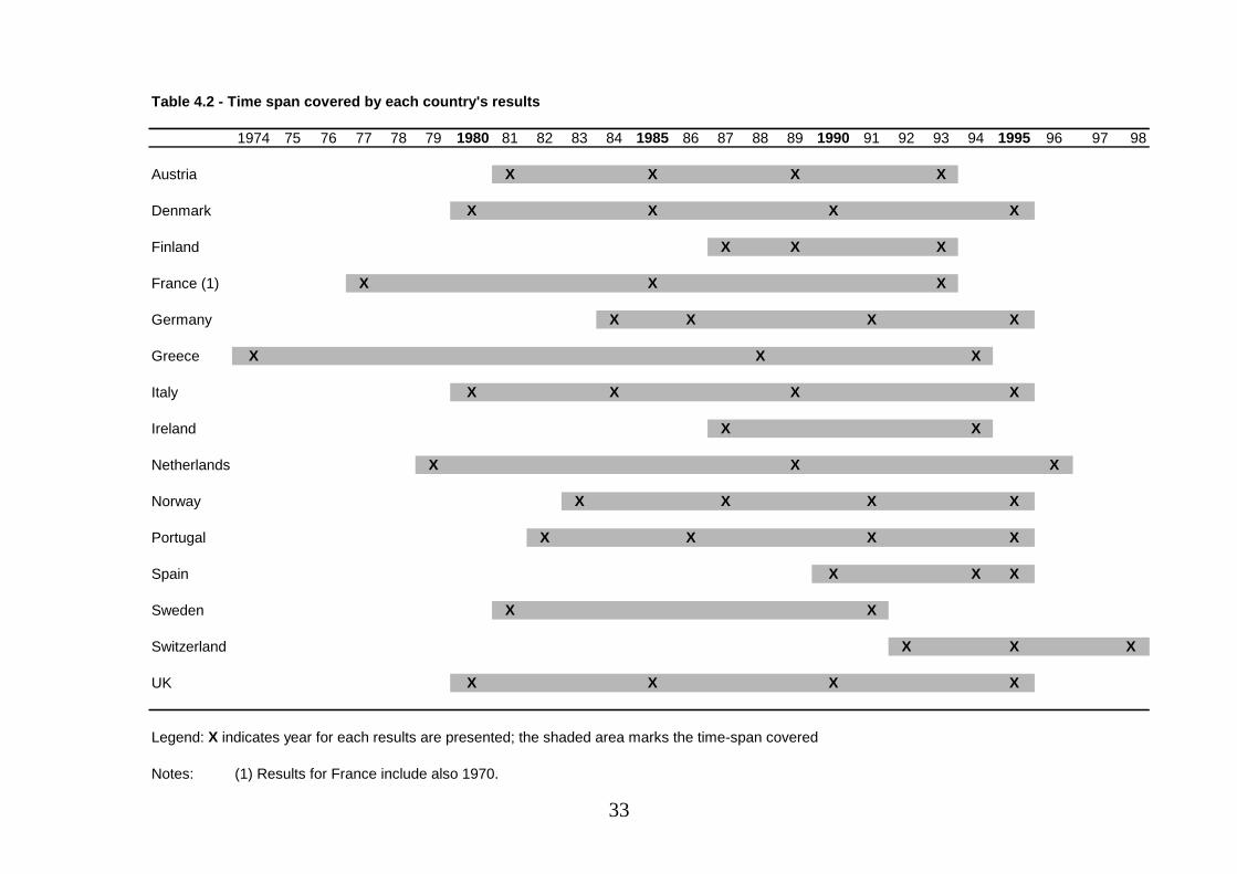
The years for which a country snap-shot is available are centred around 1980, 1985, 1990 and

1995 (see Table 4.2). However, there are still some differences in the length of the coverage,

ranging from a 24-year period in the case of French results (1970-1993) and six years for Spain

(1990-1995). There are also some countries for which data is available only from the late 1980’s

onward (Finland and Ireland) or for the 1990’s (Spain and Switzerland).

Table 4.3 provides descriptive statistics for each data-set/year used in the empirical part of the

paper. An important observation which is to be found is the increasing schooling attainment of

12

the working populations across the countries surveyed.18 Moreover, all countries have averages of

at least 10 years of schooling. The exception is Portugal, with figures substantially lower (from

4.9 to 6.5 years of schooling). Switzerland, Ireland, Netherlands, UK and Denmark boast the

highest averages (12 of more years of schooling in 1995). Aside from Portugal, Italy, Greece and

Spain have the lowest figures, reaching a maximum of 10 years in the last year.

Average experience has followed a less consistent path, as it is seen to decrease in some countries

(Austria, Greece, Italy, Portugal and UK) and increase in others (Denmark, Finland, Ireland and

Switzerland). There seems to be some convergence process, as the former countries are those

with high average experience levels (more than 20 years) while the latter have the low figures

(less than 20 years).

Descriptive statistics (means and standard deviations of log wages and three deciles of wages) are

also reported for the dependent variable used by each country. These are gross for all countries

except Austria, Greece and Italy, which use net figures. Comparisons, either within or between

countries, are difficult on account of the differences in currencies and inflation rates.19

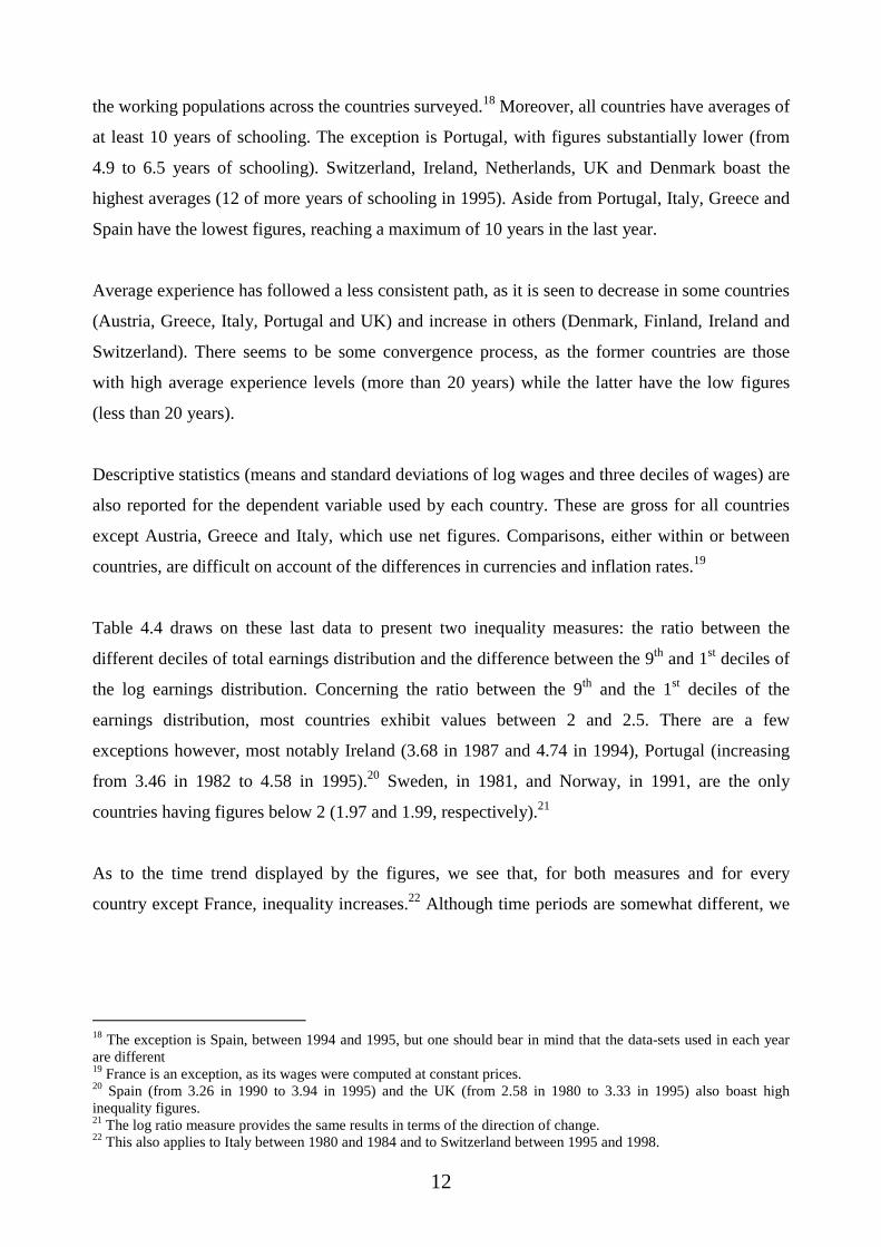
Table 4.4 draws on these last data to present two inequality measures: the ratio between the

different deciles of total earnings distribution and the difference between the 9th and 1st deciles of

the log earnings distribution. Concerning the ratio between the 9th and the 1st deciles of the

earnings distribution, most countries exhibit values between 2 and 2.5. There are a few

exceptions however, most notably Ireland (3.68 in 1987 and 4.74 in 1994), Portugal (increasing

from 3.46 in 1982 to 4.58 in 1995).20 Sweden, in 1981, and Norway, in 1991, are the only

countries having figures below 2 (1.97 and 1.99, respectively).21

As to the time trend displayed by the figures, we see that, for both measures and for every

country except France, inequality increases.22 Although time periods are somewhat different, we

18 The exception is Spain, between 1994 and 1995, but one should bear in mind that the data-sets used in each yearare different19 France is an exception, as its wages were computed at constant prices.20 Spain (from 3.26 in 1990 to 3.94 in 1995) and the UK (from 2.58 in 1980 to 3.33 in 1995) also boast highinequality figures.21 The log ratio measure provides the same results in terms of the direction of change.22 This also applies to Italy between 1980 and 1984 and to Switzerland between 1995 and 1998.

13

find these results to be in line with those of Table 1.1.23 It is interesting to note the positive

correlation between schooling attainment and inequality.

5. Empirical results

In this section we present the results obtained for fifteen European countries. Following this, we

offer an assessment of the different situations we find in terms of the link between education and

inequality. It will be seen that the overall panorama of this link is very diverse across these

countries.24

All the results described below were obtained by regressing the following version of the Mincer

equation25:

iiiii ueducyh ++++= 221 exp.exp..log θθθθ δδβα ,

where i = 1, …, N (N being the number of observations for each year), θ = .1, .2, …, .9 is the

quantile being analysed, yh is the hourly gross wage,26 educ is the number of schooling years27

and exp corresponds to Mincer experience (age minus schooling minus school starting age). Only

men working full time (35 hours or more per week) were considered.28 Each country was

considered in four separate years, which were as close as possible to 1980, 1985, 1990 and 1995.

Below we provide a summary description29 of each country’s results:

Austria (Graph 5.1): lower quantiles are associated with lower returns to education; overall

returns are falling; the slope of returns/quantiles relationship has changed somewhat, as returns to

lower quantiles have fallen while those of higher quantiles have remained unaltered.

23 The only clear exception is Portugal, for which we notice a clear rise in inequality, while Table 1.1 suggests thatthere were no significant differences in that period. This is due to the fact that Table 1.1 focuses on income, notwage, inequality. Rodrigues (1994), who decomposes income inequality into different sources, finds that if one wereto concentrate only on gross wages, one would find rising inequality.24 See Asplund and Pereira (1999) for an extensive survey of recent research in returns to education across Europe.25 This was also the version adopted throughout in the PuRE project.26 Results from Austria draw on net wages.27 For most countries only information on the highest level achieved was available. Extra school attainment above theschool years associated with the degree are disregarded.28 The situation for women was disregarded on account of the extra complication of potential selectivity biases.29 The complete results are displayed in Table 5.1.

14

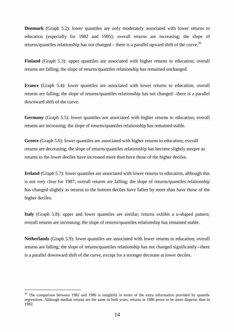
Denmark (Graph 5.2): lower quantiles are only moderately associated with lower returns to

education (especially for 1982 and 1995); overall returns are increasing; the slope of

returns/quantiles relationship has not changed – there is a parallel upward shift of the curve.30

Finland (Graph 5.3): upper quantiles are associated with higher returns to education; overall

returns are falling; the slope of returns/quantiles relationship has remained unchanged.

France (Graph 5.4): lower quantiles are associated with lower returns to education; overall

returns are falling; the slope of returns/quantiles relationship has not changed –there is a parallel

downward shift of the curve.

Germany (Graph 5.5): lower quantiles are associated with higher returns to education; overall

returns are increasing; the slope of returns/quantiles relationship has remained stable.

Greece (Graph 5.6): lower quantiles are associated with higher returns to education; overall

returns are decreasing; the slope of returns/quantiles relationship has become slightly steeper as

returns to the lower deciles have increased more than have those of the higher deciles.

Ireland (Graph 5.7): lower quantiles are associated with lower returns to education, although this

is not very clear for 1987; overall returns are falling; the slope of returns/quantiles relationship

has changed slightly as returns to the bottom deciles have fallen by more than have those of the

higher deciles.

Italy (Graph 5.8): upper and lower quantiles are similar; returns exhibit a u-shaped pattern;

overall returns are increasing; the slope of returns/quantiles relationship has remained stable.

Netherlands (Graph 5.9): lower quantiles are associated with lower returns to education; overall

returns are falling; the slope of returns/quantiles relationship has not changed significantly –there

is a parallel downward shift of the curve, except for a stronger decrease at lower deciles.

30 The comparison between 1982 and 1986 is insightful in terms of the extra information provided by quantileregressions. Although median returns are the same in both years, returns in 1986 prove to be more disperse than in1982.

15

Norway (Graph 5.10): lower quantiles are associated with lower returns to education; overall

returns are increasing; the slope of returns/quantiles relationship has not changed significantly –

there is a parallel upward shift of the curve.

Portugal (Graph 5.11): lower quantiles are associated to lower returns to education; overall

returns are increasing; the slope of returns/quantiles relationship has changed markedly –returns

to lower quantiles have fallen while returns to upper quantiles have increased.

Spain (Graph 5.12): lower quantiles are associated to lower returns to education; overall returns

are increasing; the slope of returns/quantiles relationship has not changed –there is a parallel

upward shift of the curve.

Sweden (Graph 5.13): upper quantiles are clearly associated with higher returns to education;

overall returns are decreasing; the slope of returns/quantiles relationship has changed slightly –

returns to lower quantiles have fallen slightly more than have returns to upper quantiles; returns

to lower quantiles are particularly low (2%-3%).

Switzerland (Graph 5.14): upper quantiles are associated with higher returns to education;

overall returns fall slightly; the slope of returns/quantiles relationship has changed slightly –

returns to upper quantiles have remained stable while those of lower quantiles have fallen.

United Kingdom (Graph 5.15): upper quantiles are associated with higher returns to education;

overall returns are increasing; the slope of the returns/quantiles relationship has remained stable.

We present in Table 5.2 and Graph 5.16 the returns to education (in percentage terms) for the

lower and top deciles and for the first and last year considered by each country (approximately

1980 and 1995, although there are a few exceptions). It can be seen that returns differ greatly

across the fifteen countries surveyed (and the 15-year period considered). They range between

12.6% (Portugal, 1995) and 4.1% (Sweden, 1995).

Considering as a threshold between large and small an 8% return, the high-return countries are

Austria, Finland, Ireland, Portugal and Switzerland, while the low-return countries are Denmark,

16

France, Greece, Italy, Norway and Sweden.31 There is thus some evidence of convergence in

returns to education as returns to high-return countries have been falling, whereas the opposite

occurs for low-return countries.32,33

Some results obtained from the quantile regressions run for each country are presented in Table

5.3. The first column presents the difference between OLS returns to education estimates at those

years. The panorama here is very diverse: Denmark, Greece, Italy, Norway, Portugal and the UK

have increasing returns, while Austria, Finland, Germany, Ireland, Sweden and Switzerland have

falling returns. The greatest increase is Italy (2.1%) while the biggest fall is Ireland (-2.7%).

There might be some convergence phenomenon as the high-return countries see such returns fall

while the opposite occurs for the low-return countries. The exceptions in this process are Sweden

and Portugal.

The following two columns refer to the differences in returns to education for the same quantiles

between 1980 and 1995. Column 2 [Q(.1|95)-Q(.1|80)], which considers returns to the first decile,

measures how different the pay-off to education for the low-earnings individuals became in the

15-year period under consideration. Austria, Finland, Germany, Ireland, Portugal, Sweden and

Switzerland have negative figures here. This result suggests that, for these seven countries, the

role of education for the less attractive to the labour market has been eroded during the last two

decades. Moreover, it is insightful to compare the evolution of returns at the mean (OLS) and at

the first decile (QR) and notice that, in most countries (the exceptions are Finland, France, Italy

and the UK), the former returns (OLS) always exceed the latter.

The same computations (the difference between 1995 and 1980 results) were applied to the top

quantile (column 3). Here we find negative figures for Finland, France, Germany, Ireland,

Sweden and Switzerland. This means that, in these countries, returns to education have fallen

across those individuals who reap the highest earnings at each educational level. On the other

hand, if we compare columns 2 and 3, we see that returns to the bottom quantile have fallen by

more (or increased by less) than their top quantile counterparts in all countries except for France,

Germany, Italy and the UK. This means that, for the majority of countries, the downward

(upward) pressure in returns to education at the bottom quantile is stronger (weaker) than at the

31 Netherlands, Spain and the UK have values above or below this threshold depending on the year considered.32 The only exceptions are Portugal and Sweden.33 See the last rows of table 5.2 where the coefficient of variation of OLS returns falls from 0.31 to 0.26 from the firstto the last years considered.

17

top quantile. Moreover, with respect to the evolution of OLS and Quantile Regressions returns,

returns at the ninth decile have increased by more (or decreased by less) than those at the mean in

every country (except Denmark and France).

In columns 4 and 5, we compare different quantiles in the same year (and not the same quantiles

in different years, as before). Except for Germany and Greece, the return for the top quantile is

always larger than the return for the lower quantile. Moreover, taking into account column 5, we

see that the difference in returns across the earnings distribution is always higher in 1995 than in

1980 (except for France, Germany, Greece, Italy and the UK).34 This means that the different role

of education upon wages across the wage distribution has become more acute, in the sense that

the richer (at each educational level) are benefiting increasingly more from it than the poorer. We

may thus conclude that, in some European countries, returns to education have fanned out.

Following upon this, one must conclude that these fifteen countries exhibit different situations.

However, a few similarities among them may be found and used in order to draw the countries

together into some specific types.

Bearing these results in mind, we defined four groups of countries –see Table 5.3. In the first

group, which includes only Portugal, returns increase markedly along the conditional wage

distribution and this trend has become more pronounced in recent years. Moreover, the returns to

the top deciles have been increasing while the opposite has taken place for the bottom deciles.

Not only is the role of education increasingly more important for the top deciles, for the bottom

deciles the importance of that role has fallen in the 15-year period covered.

Our second type is formed with Austria, Finland, France, Ireland, Netherlands, Norway, Spain,

Sweden, Switzerland and the UK. As mentioned above, returns in these countries increase with

the wage distribution. However, and contrary to the previous type, there has been no clear

increase in dispersion going on: the slope of the returns-deciles curve has not changed

significantly.35,36 Therefore, although education also contributes to further inequality in this set of

countries, its influence has not been increasing as clearly as in the previous group.

34 Portugal is the most extreme case as such difference more than doubles, jumping from 3.7% to 8.9%.35 This conclusion does not fully apply to Austria and Sweden, where we see falling returns for those at the lowerdeciles while returns to upper quantiles remain unaltered. These two countries could also be placed in the firstcategory.

18

In the third group, Denmark and Italy, returns are approximately the same along the conditional

wage distribution. This means that, in Denmark and Italy, the educational impact on inequality

should be light, as only the effect of inter-education inequality (related to positive returns to

education) is present.

Finally, in a fourth type made up of Germany and Greece, we observe higher returns for those at

the bottom deciles of the conditional earnings distribution –the slope of the returns-quantiles

relationship is negative. This contrasts with the previous three situations, where the relationship

was clearly positive (or horizontal). Education, in these countries, reduces intra-education

inequality, as the contribution of education upon the less labour-market attractive is stronger than

upon the most attractive. Nevertheless, as mentioned in Section 3, it may happen that the inter-

education inequality effect dominates, thus resulting in an overall positive effect of education

upon inequality.37

It should also be mentioned that out of the four countries which do not follow the predominant

pattern of increasing returns in the conditional distribution, the results for two of them (Italy and

Greece) are based on net wages. This should result in a less steep returns-quantiles profile as

progressive taxes should contribute to smoothing returns at higher quantiles.

The overall information present here is summarised in Graph 5.17. Here we restrict our analysis

to the situations facing each country in 1980 and 1995 (or the closest years available). On the x-

axis we consider returns to the first decile, while the y-axis depicts returns to the ninth decile.

Each point corresponds to the case of each country in one of such years. Results for each country

are then connected and a small arrow indicates the direction of the ‘movement’, from the

beginning of the 1980’s until the mid-1990’s.38

A 45º-degree line was also included, representing the loci where point estimates of the returns to

the first decile and to the ninth decile are equal. This line also separates the graph in two halves.

The top, left-hand-side part includes those countries whose returns to education are higher for the

36 This situation corresponds to the case of the USA –see Buchinsky (1994).37 See Tsakloglou and Antoninis (1999) for an analysis of the impact of public education upon inequality in Greece.The authors conclude that such impact is negative, especially in terms of the primary and secondary levels. Theirapproach is very different from the one taken in this paper, as they focus on education-related government transfersto households, and not on education-related wage income.38 When the years were three or more years different from these, the true years were inserted next to thecorresponding point.

19

highest decile than for the lowest.39 All countries surveyed can be found in this sub-set, except for

Germany40 and Greece. Denmark and Italy are also close enough to the border that each country’s

returns at each year are statistically equal.41

All the remaining countries, which in the previous classification were placed in the first two

groups, can be found in the upper left part of the graph. These countries thus have returns to

education which are higher for the top deciles than for the lower deciles.

Another piece of information displayed in this graph is the trend in returns to education at each

extreme of the distribution of earnings. Positively-sloped segments correspond to situations

where the returns to both the ninth and the first decile are moving in the same way, either

increasing or falling. This is the case of all countries, except for Austria, France and Portugal. For

these three countries returns at different parts of the distribution are moving in opposite

directions.42

However, differences in France are not statistically significant, while in Austria only the returns

to the first deciles are statistically different. This leaves us with Portugal as the only country

where returns at each end of the distribution are moving in opposite ways. The returns at opposite

quantiles of the distribution are diverging because the lowest returns (for the bottom decile) are

falling, while the higher returns (to the highest decile) are getting even higher.43

An interesting way to interpret these overall results is to assume that the only unobserved variable

is ability (or motivation) and the education decision is exogenous (not influenced by ability). If

this were so, then an OLS regression would produce returns to education for individuals with

mean unobserved ability. On the other hand, the results from quantile regressions provide

estimates for returns to education for individuals at different percentiles of the ability distribution.

39 The threshold for statistical difference of point estimates adopted was one standard deviation.40 Results for the first period (1984) are not statistically different, however. In this year returns to the lowest quantilewere not significantly higher than those of the highest quantile.41 This is not true for Denmark in 1995, when returns to the top quantile are higher than returns to the lower quantile.We opted to include this country in this sub-set as the difference is small and the situation applies for 1980.42 The returns for Finland and Sweden (only for the ninth decile) are also not significantly different.43 It could be argued that Austria should also be included in the first group, as the returns/deciles relationship is notpositively sloped as for the second group countries. However, since the relationship is not significantly negativelyshaped, we opted for classifying Austria as we did.

20

To the extent that this assumption holds, the contrasting results obtained must be explained by

differences in the way that the education system and/or the labour market of each country deal

with individuals with different abilities or by differences in the degree of interaction between

schooling and ability. It is then the case that in countries of the third and fourth types (zero- and

negatively-sloped returns-deciles curves) the functioning of such institutions44 compensates for

the lower ability of some individuals so that there is no such interaction.

On the other hand, such mechanisms are not in place in countries of the first and second types

(positively-sloped returns-deciles curves), who represent a overwhelming majority in our

sample.45 In this case, and given the assumptions above, there is a positive interaction between

schooling and ability, whereby schooling exacerbates ability-related differences. This is a result

in line with those of ‘The Bell curve’ (Herrnstein and Murray (1995)) where cognitive ability is

seen as the main force explaining social and economic differences.

6. Conclusions

The link between education and inequality is tackled in this paper by considering results from

quantile regressions of Mincer/wage equations from fifteen European countries across an

approximately fifteen-year period (from 1980 until 1995).

We use this methodology after decomposing the effect of education upon inequality in three

terms: inequality due to within- and to between-educational-levels earnings differentials (prices)

and to changes in the distribution of schooling (quantities). The first term is associated with the

positive returns to education which entail that, on average, more educated individuals earn more,

while the second term deals with the different dispersions of conditional distributions of earnings

across different educational levels.

By running Mincer equations with the quantiles regression technique, we perceived four different

situations. The first case was that of Portugal, where not only do returns increase with the

quantiles of the conditional earnings distribution, but the relationship has become more acute

44 The above-mentioned institutions might comprise specific wage-bargaining systems, special training or vocationalsystems at the upper secondary level and minimum wage laws.

21

over time. This suggests a positive and increasing impact of education upon inequality, in the

sense that within-levels inequality exists and has been increasing.

In a second case (Austria, Finland, France, Ireland, Netherlands, Norway, Spain, Sweden,

Switzerland and the UK) a positive but stable relationship was found. The third group included

Denmark and Italy, for whom returns are very similar across the distribution, a result which

means that education has neither increased nor decreased inequality. Finally, in a fourth case,

Germany and Greece, the returns-quantiles profile is negative, which suggests that, as far as

within-levels inequality is concerned, education reduces inequality.

Overall, these international differences provide a summary assessment of the outcome of the

interaction between education systems and labour-market institutions in each country in terms of

wage inequality. Our results prove that such a process works differently across the fifteen-country

sample of European countries considered.

However, for a majority of such countries (Austria, Finland, France, Ireland, Netherlands,

Norway, Portugal, Spain, Sweden, Switzerland and the UK), one sees very clearly that the

dispersion in earnings increases with the educational levels. In these countries difficult-to-

measure individual-specific characteristics (e.g., motivation or ability) play a larger role in

earnings than in the remaining countries.

If we assume that such characteristics can be proxied by ability then our results say that there is a

positive interaction between ability and education: the higher the ability level, the stronger will

the impact of schooling be on one’s wages. This result supports ‘Bell curve’ type of arguments

which place much emphasis on the role of cognitive ability on economic and social success.

On the other hand, to the extent that prospective students are unaware of their own endowments

of such characteristics, this result implies that the risk associated with educational investments is

greater in those countries. This is also associated with over-education, in the sense that the

marginal reward some individuals reap from their schooling is very low or even negative.

45 A possible explanation of these results is that there is some interaction between experience and education whichtakes place at higher wages. This possibility was tested in the case of Portugal but no evidence was found to supportit.

22

In terms of policy-making, these overall results should be useful as they amount to a summary

characterisation of the joint functioning of each country’s national education system and labour-

market institutions. Should wage equality be considered to be a political goal, a country where

such joint mechanism promotes inequality might wish, on both efficiency and equity grounds, to

pinpoint and reverse the underlying causes.

7. References

Abadie, A., J. Angrist and G. Imbens (1999) ‘Instrumental variables estimates of the effect of

subsidized training on the quantiles of trainee earnings’, mimeo, MIT.

Asplund, R. and P. Pereira (1999) ‘Returns to human capital in Europe: a literature review’,

ETLA, Helsinki.

Blau, F. and L. Kahn (1996) 'International differences in male wage inequality: institutions versus

market forces', Journal of Political Economy, 104, 791-837.

Buchinsky, M. (1994) ‘Changes in the US wage structure, 1963-1987: application of quantile

regression’, Econometrica, 62, 405-458.

Buchinsky, M. (1995a) ‘Quantile regression, Box-Cox transformation model, and the US wage

structure, 1963-1987', Journal of Econometrics, 65, 109-154.

Buchinsky, M. (1995b) ‘Recent advances in Quantile regression models', Journal of Human

Resources, 33, 88-126.

Card, D. (1994) ‘Earnings, schooling, and ability revisited’, National Bureau of Economic

Research Working Paper 4832.

Card, D. (1999) ‘The causal effect of education on earnings’, forthcoming in the Handbook of

Labour Economics, vol. 3, edited by O. Ashenfelter and D. Card, North-Holland, Amsterdam.

23

Cardoso, A. (1998) ‘Earnings inequality in Portugal: high and rising?’, Review of Income and

Wealth, 44, 325-343.

Champernowne, D. and F. Cowell (1998) 'Economic inequality and income distribution',

Cambridge, Cambridge University Press.

Juhn, C., K. Murphy and B. Pierce (1993) ‘Wage inequality and the rise in returns to skill’,

Journal of Political Economy, 101, 3.

Fersterer, J. and R. Winter-Ebmer (1999) ‘Are Austrian returns to education falling over time?’,

University of Linz. [www.economics.uni-linz.ac.at/Paper/papers/returns_falling11a.pdf]

Garcia, J., P. Hernandez and A. López (1997) ‘How wide is the gap? An investigation of gender

wage differences using quantile regression’, mimeo, Universitat Pompeu Fabra.

Greene, W. ‘Econometric analysis’, Prentice-Hall, New Jersey.

Gottschalk, P. and T. Smeeding (1997) ‘Cross-national comparisons of earnings and income

inequality’, Journal of Economic Literature, 35, 633-687.

Gottschalk, P. (1997) ‘Inequality, income growth, and mobility: the basic facts’, Journal of

Economic Perspectives, 11, 21-40.

Hartog, J., Pedro T. Pereira and José C. Vieira (1999) ‘Changing returns to education in Portugal

during the 1980s and early 1990s: OLS and quantile regression estimators’, WP 336, Faculdade

de Economia da Universidade Nova de Lisboa.

[www.fe.unl.pt/FE/content/serv/servdoc/ban/WPFEUNL/Wp1999/WP336.doc]

Heckman, J. (1999) ‘Policies to foster human capital’, NBER Working Paper 7288.

Herrnstein, R. and C. Murray (1995) ‘The Bell curve: intelligence and class structure in

American life’, Free Press, New York.

24

Ichino, A. and R. Winter-Ebmer (1998) ‘The long-run educational cost of World War II: an

example of local average treatment effect estimation’, CEPR discussion paper 1895.

Imbens, G. and J. Angrist (1994) ‘Identification and estimation of local average treatment

effects’, Econometrica, 62, 467-476.

Katz, L. and K. Murphy (1992) 'Changes in relative wages, 1963-1987: supply and demand

factors', Quarterly Journal of Economics, 107, 35-78.

Koenker, R. and G. Bassett (1978) ‘Regression quantiles’, Econometrica, 46, 33-50.

Koenker, R. and G. Bassett (1982) ‘Robust tests for heteroscedasticity based on regression

quantiles’, Econometrica, 50, 43-61.

Lee, D. (1999) ‘Wage inequality in the United States during the 1980s: rising dispersion or

falling minimum wage?’, Quarterly Journal of Economics, 112, 977-1023.

Leuven, E., H. Oosterbeek and H. van Ophen (1997) 'Explaining international differences in male

wage inequality by differences in demand and supply of skill', mimeo.

Machado, J. F. and J. Mata (1998) ‘Earnings function in Portugal, 1982-1994: evidence from

quantile regressions’, WP 2-98, Banco de Portugal.

Mata, J. and J. Machado (1996) ‘Firm start-up size: a conditional quantile approach’, European

Economic Review, 40, 1305-1323.

Mosteller, F. and J. Tukey (1977) ‘Data analysis and regression’, Addison-Wesley, Reading, MA.

OECD (1995) ‘Income distribution in OECD countries’, Social Policy Studies No. 18, Paris.

OECD (1998) ‘Education at a glance: OECD indicators’, Centre for Educational Research and

Innovation, Paris.

Oliveira Martins, G. (1999) Address to UNESCO, UNESCO, Paris.

25

Pereira, P. and P. Martins (2000) ‘Returns to education in Portugal, 1982-1999: high and rising’,

mimeo, Faculdade de Economia da Universidade Nova de Lisboa.

Rodrigues, C. (1994) ‘Repartição do rendimento e desigualdade: Portugal nos anos 80’, Estudos

de Economia, 14, 399-428.

Tsakloglou, P. and M. Antoninis (1999) ‘On the distributional impact of public education:

evidence from Greece’, Economics of Education Review, 18, 439-452.

Welch, F. (1999) 'In defence of inequality', American Economic Review, 89, 1-17 (Papers and

Proceedings).

26

Table 1.1 - Changes in market income inequality

Country Years Change Market Income InequalityUK 1981-91 +++USA 1980-93 +++Sweden 1980-93 +++Australia 1980-81 +Denmark 1980-90 +New Zealand 1981-89 +Japan 1981-90 +Netherlands 1981-89 +Norway 1982-89 +Belgium 1985-92 +Canada 1980-92 +Israel 1979-92 +Finland 1981-92 +++France 1979-89 0Portugal 1980-90 0Spain 1980-90 naIreland 1980-87 +West Germany 1983-90 +Italy 1977-91 -

Designation: Interpretation: Range of change in Gini- small decline -5% or more0 zero -4% to +4%+ small increase 5% to 10%

++ moderate increase 10% to 15%+++ large increase 16% to 29%

Source: Gottschalk and Smeeding (1997), table 4, page 666

27

Table 2.1 - Gender distribution of hourly earnings

Income IncomeClass %obs tot% %obs tot% Class %obs tot% %obs tot%

5.2 0.0% 0.0% 0.0% 0.0% 7.24 0.5% 94.1% 0.9% 88.5%5.24 0.0% 0.0% 0.0% 0.0% 7.28 0.5% 94.6% 0.9% 89.4%5.28 0.0% 0.0% 0.0% 0.0% 7.32 0.5% 95.0% 0.8% 90.2%5.32 0.1% 0.1% 0.1% 0.1% 7.36 0.4% 95.5% 0.8% 91.0%5.36 0.2% 0.3% 0.1% 0.2% 7.4 0.4% 95.9% 0.8% 91.8%5.4 0.3% 0.6% 0.2% 0.4% 7.44 0.4% 96.3% 0.7% 92.5%

5.44 0.3% 0.9% 0.2% 0.6% 7.48 0.3% 96.6% 0.5% 93.0%5.48 0.3% 1.2% 0.2% 0.8% 7.52 0.3% 96.9% 0.5% 93.5%5.52 0.3% 1.5% 0.2% 1.0% 7.56 0.2% 97.1% 0.5% 94.1%5.56 0.5% 2.1% 0.3% 1.3% 7.6 0.3% 97.4% 0.4% 94.5%5.6 0.8% 2.8% 0.5% 1.8% 7.64 0.2% 97.6% 0.5% 95.0%

5.64 3.5% 6.4% 1.9% 3.7% 7.68 0.2% 97.8% 0.4% 95.3%5.68 3.2% 9.6% 1.5% 5.2% 7.72 0.2% 98.1% 0.4% 95.7%5.72 5.1% 14.7% 2.0% 7.2% 7.76 0.2% 98.3% 0.4% 96.1%5.76 3.6% 18.3% 1.7% 8.9% 7.8 0.2% 98.4% 0.3% 96.4%5.8 4.5% 22.8% 2.0% 10.9% 7.84 0.1% 98.5% 0.3% 96.7%

5.84 5.7% 28.5% 1.9% 12.8% 7.88 0.2% 98.7% 0.3% 97.0%5.88 5.7% 34.2% 2.5% 15.3% 7.92 0.1% 98.8% 0.2% 97.2%5.92 5.6% 39.8% 2.3% 17.6% 7.96 0.2% 99.0% 0.3% 97.5%5.96 4.2% 44.0% 2.8% 20.4% 8 0.1% 99.2% 0.2% 97.8%

6 3.5% 47.5% 3.0% 23.4% 8.04 0.1% 99.3% 0.3% 98.0%6.04 3.5% 51.1% 3.3% 26.7% 8.08 0.1% 99.4% 0.2% 98.2%6.08 3.2% 54.3% 3.1% 29.8% 8.12 0.0% 99.4% 0.2% 98.4%6.12 3.0% 57.2% 3.0% 32.8% 8.16 0.1% 99.5% 0.1% 98.6%6.16 2.9% 60.1% 3.2% 36.0% 8.2 0.1% 99.5% 0.2% 98.7%6.2 2.7% 62.8% 4.1% 40.1% 8.24 0.0% 99.6% 0.1% 98.9%

6.24 2.6% 65.4% 3.3% 43.4% 8.28 0.0% 99.6% 0.1% 99.0%6.28 2.6% 68.0% 3.2% 46.6% 8.32 0.0% 99.6% 0.1% 99.1%6.32 2.2% 70.2% 2.8% 49.5% 8.36 0.1% 99.7% 0.1% 99.2%6.36 2.0% 72.1% 2.7% 52.2% 8.4 0.0% 99.7% 0.1% 99.3%6.4 2.1% 74.2% 2.4% 54.6% 8.44 0.0% 99.8% 0.1% 99.4%

6.44 1.6% 75.8% 2.6% 57.1% 8.48 0.0% 99.8% 0.1% 99.5%6.48 1.4% 77.3% 2.3% 59.4% 8.52 0.0% 99.8% 0.1% 99.5%6.52 1.4% 78.7% 2.2% 61.6% 8.56 0.0% 99.8% 0.1% 99.6%6.56 1.5% 80.2% 2.1% 63.7% 8.6 0.0% 99.9% 0.0% 99.6%6.6 1.1% 81.3% 1.9% 65.6% 8.64 0.0% 99.9% 0.0% 99.7%

6.64 1.2% 82.5% 1.9% 67.4% 8.68 0.0% 99.9% 0.0% 99.7%6.68 1.1% 83.6% 1.9% 69.3% 8.72 0.0% 99.9% 0.0% 99.7%6.72 1.0% 84.6% 1.8% 71.1% 8.76 0.0% 99.9% 0.1% 99.8%6.76 0.9% 85.5% 1.7% 72.8% 8.8 0.0% 99.9% 0.0% 99.8%6.8 0.9% 86.3% 1.8% 74.6% 8.84 0.0% 99.9% 0.0% 99.8%

6.84 0.8% 87.1% 1.4% 76.0% 8.88 0.0% 100.0% 0.0% 99.9%6.88 0.6% 87.7% 1.4% 77.5% 8.92 0.0% 100.0% 0.0% 99.9%6.92 0.8% 88.5% 1.4% 78.8% 8.96 0.0% 100.0% 0.0% 99.9%6.96 0.9% 89.4% 1.4% 80.3% 9 0.0% 100.0% 0.0% 99.9%

7 0.7% 90.1% 1.4% 81.7% 9.04 0.0% 100.0% 0.0% 99.9%7.04 0.7% 90.8% 1.3% 83.0% 9.08 0.0% 100.0% 0.0% 99.9%7.08 0.7% 91.6% 1.2% 84.1% 9.12 0.0% 100.0% 0.0% 99.9%7.12 0.7% 92.3% 1.2% 85.4% 9.16 0.0% 100.0% 0.0% 100.0%7.16 0.6% 92.9% 1.1% 86.4% 9.2 0.0% 100.0% 0.0% 100.0%7.2 0.7% 93.5% 1.1% 87.6%

Notes: Right tail of the distribution not describedBold and underlined: modal class; Italics: classes associatedwith each decileSource: Quadros de Pessoal , 1995 sample.

Men WomenMen Women

WomenMen

0%

1%

2%

3%

4%

5%

6%

Log Hourly Earnings

Graph 2.1 - Distribution of log hourly earnings, Portugal, 1995, Men and Women

Women Men

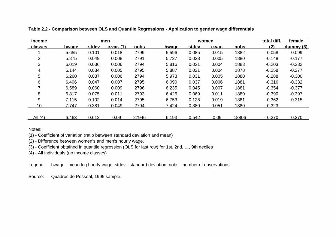
Table 2.2 - Comparison between OLS and Quantile Regressions - Application to gender wage differentials

income total diff. femaleclasses hwage stdev c.var. (1) nobs hwage stdev c.var. nobs (2) dummy (3)

1 5.655 0.101 0.018 2799 5.596 0.085 0.015 1882 -0.058 -0.0992 5.875 0.049 0.008 2791 5.727 0.028 0.005 1880 -0.148 -0.1773 6.019 0.036 0.006 2794 5.816 0.021 0.004 1883 -0.203 -0.2324 6.144 0.034 0.005 2795 5.887 0.021 0.004 1878 -0.258 -0.2775 6.260 0.037 0.006 2794 5.973 0.031 0.005 1880 -0.288 -0.3006 6.406 0.047 0.007 2795 6.090 0.037 0.006 1881 -0.316 -0.3327 6.589 0.060 0.009 2796 6.235 0.045 0.007 1881 -0.354 -0.3778 6.817 0.075 0.011 2793 6.426 0.069 0.011 1880 -0.390 -0.3979 7.115 0.102 0.014 2795 6.753 0.128 0.019 1881 -0.362 -0.31510 7.747 0.381 0.049 2794 7.424 0.380 0.051 1880 -0.323

All (4) 6.463 0.612 0.09 27946 6.193 0.542 0.09 18806 -0.270 -0.270

Notes:(1) - Coefficient of variation (ratio between standard deviation and mean)(2) - Difference between women's and men's hourly wage.(3) - Coefficient obtained in quantile regression (OLS for last row) for 1st, 2nd, …, 9th deciles(4) - All individuals (no income classes)

Legend: hwage - mean log hourly wage; stdev - standard deviation; nobs - number of observations.

Source: Quadros de Pessoal, 1995 sample.

men women

Table 4.1a - Data-sets description

Country Data-set Description Years Obs. Outliers cleaning procedure (1)

Austria Mikrozensus 1% Household Survey 1981 9889 Employees with wages below minimum(net wages) 1985 8120 Social Security contribution level

1989 7878 (US$ 320 at 1993 level)1993 7175 Employees below 15 or above 65 years

Denmark LLMR Longitudinal Labour Market 1980 4099 None Register (0.5% sample) 1985 4212

1990 43521995 4416

Finland Labour Force Cross-section labour 1987 1888 Extremely high and low earnersSurvey force survey 1989 2089 Zero earnings and zero hours

1993 1175

France FQP Cross-section household 1970 15297 Wages below minimum wage and survey 1977 14227 extremely high wages

1985 122451993 4606

Germany GSOEP 1984198619911995

Greece EOP Household Budget Survey 1974 2267 Zero earning and zero hours, more than(net wages) 1988 1860 84 hours per week, aged below 14 or

1994 2096 above 64, primary sector

Ireland ESRI Cross-section household data 1987 18951994 1903

Italy SHIW Cross-section household- 1980 1730 Observations without earningsbased dataset 1984 2200 (missing or equal to zero)

1989 41141995 3441

Notes: (1) - Observations which were dropped

32

Table 4.1b - Data-sets description

Country Data-set Description Years Obs. Outliers cleaning procedure (1)

Netherlands Structure of earnings Cross-section employer- 1979 40726 Unknown (Statistical agency's survey based dataset 1989 12555 responsibility)

1996 49805

Norway Level of living survey 1983 1037 Earnings below 20 NOK and1987 970 above 1000 NOK1991 9011995 870

Portugal Quadros Cross-section employer- 1982 27019 Zero earning and zero hoursde Pessoal based data-set 1986 26595

1991 279521995 28055

Spain Household Budget S. 1990 9714ECHP 1994 2181Wage Structure S. 1995 118005

Sweden Swedish Level Cross-sectional data 1981 1658 Zero earningsof Living Surveys (representative of Swedes) 1991 1508

Switzerland Swiss Labour Cross section of the adult 1992 3388 0.5% at the bottom and the topForce Survey population permantently residen 1995 6334 of the wage distribution

in Switzerland 1998 3275

UK Family Expenditures Longitudinal household survey 1980 2883 Zero earnings and zero hoursSurvey focused on expenditures 1985 2526 Hourly earnings below 1 GBP

1990 24251995 2183

Notes: (1) - Observations which were dropped

33

Table 4.2 - Time span covered by each country's results

1974 75 76 77 78 79 1980 81 82 83 84 1985 86 87 88 89 1990 91 92 93 94 1995 96 97 98

Austria X X X X

Denmark X X X X

Finland X X X

France (1) X X X

Germany X X X X

Greece X X X

Italy X X X X

Ireland X X

Netherlands X X X

Norway X X X X

Portugal X X X X

Spain X X X

Sweden X X

Switzerland X X X

UK X X X X

Legend: X indicates year for each results are presented; the shaded area marks the time-span covered

Notes: (1) Results for France include also 1970.

34

Table 4.3a - Descriptive statistics

Country Years Educ. (1) Exp. (2) Mean St.Dev. 1st dec. 5th dec. 9th dec.

Austria 1981 9.5 22.2 3.99 0.34 37.5 50.0 81.31985 9.7 21.4 4.16 0.34 43.7 62.5 97.51989 9.8 21.3 4.35 0.34 52.6 75.0 118.71993 10.1 21.3 4.57 0.35 65.8 93.8 150.0

Denmark 1980 11.5 18.6 4.42 0.34 59.1 80.7 127.11985 11.7 18.9 4.62 0.33 71.5 97.5 151.41990 11.9 19.2 4.92 0.35 94.6 131.6 214.91995 12.0 19.4 4.97 0.36 96.5 138.4 230.4

Finland 1987 11.0 17.7 3.81 0.37 29.9 43.6 73.71989 11.1 18.4 4.02 0.37 36.1 53.8 90.91993 11.4 19.5 4.16 0.38 41.9 62.1 106.1

France (4) 1970 9.8 21.8 10.61 0.46 13.2 21.6 45.11977 10.5 20.2 10.87 0.42 17.9 28.8 53.81985 11.3 19.1 10.91 0.39 19.2 29.7 53.71993 11.4 21.9 10.92 0.39 19.8 29.8 54.1

Germany

Greece 1974 7.82 23.41 3.57 0.551988 9.89 21.55 6.11 0.471994 10.14 21.87 6.93 0.64

Ireland 1987 11.5 20.4 1.48 0.52 2.2 4.4 8.31994 12.4 23.8 1.74 0.61 2.5 5.9 11.9

Italy 1980 8.8 24.3 1.24 0.42 2.2 3.6 5.21984 9.2 23.6 1.84 0.39 4.4 6.5 9.41989 9.8 22.9 2.26 0.32 6.5 9.4 13.91995 10.1 22.9 2.52 0.41 7.8 12.5 20.8

Log Wage (3) Wage

Table 4.3b - Descriptive statistics

Country Years Educ. (1) Exp. (2) Mean St.Dev. 1st dec. 5th dec. 9th dec.

Netherlands 1979 11.5 20.3 2.88 0.43 11.4 16.4 33.71989 11.7 19.6 3.01 0.37 13.8 19.6 32.91996 12.5 20.0 3.23 0.46 15.5 24.9 43.8

Norway 1983 11.2 21.3 3.96 0.30 37.9 51.7 78.21987 11.5 19.8 4.31 0.32 51.4 73.6 109.21991 11.9 21.8 4.53 0.30 68.4 92.0 136.21995 12.2 20.9 4.65 0.33 71.4 101.1 158.0

Portugal 1982 4.9 25.1 4.58 0.52 56 92 1941986 5.3 26.0 5.35 0.56 118 191 4711991 5.9 25.3 6.06 0.59 228 379 9791995 6.5 24.5 6.42 0.61 318 531 1456

Spain (5) 1990 7.3 25.0 14.37 0.46 555.8 924.6 1809.81994 9.8 24.8 7.61 0.49 1104.5 1955.5 3813.61995 8.8 26.0 7.30 0.52 761.0 1410.3 2998.6

Sweden 1981 10.7 21.7 3.67 0.30 29.0 37.0 57.01991 11.8 21.5 4.45 0.31 61.0 81.0 127.0

Switzerland 1992 13.1 19.3 3.57 0.39 23.1 34.4 58.11995 13.2 19.8 3.60 0.40 23.9 35.9 60.31998 13.3 20.3 3.63 0.38 25.1 36.8 60.8

UK 1980 11.0 24.8 1.79 0.40 3.8 5.9 9.81985 11.4 23.8 1.87 0.44 3.9 6.3 11.21990 11.9 23.1 1.98 0.48 4.1 7.1 13.01995 12.3 22.6 2.00 0.49 4.1 7.3 13.5

Notes: (1) - Average education years in each sample (2) - Average years of experience(3) - For all countries except Austria, Italy and Greece the dependent variable was log gross wages.(4) - Log Wages refer to yearly earnings. Wages refer to hourly wages (assuming 1760 hours worked per year). All results are in 1980 francs.(5) - Results for 1990 are based in yearly earnings. Hourly wages for that year were computed assuming 1760 hoursworked per year.

Log Wage (3) Wage

Table 4.4a - Inequality computations

Log WageCountry Years 9/1 9/5 5/1 Diff. (2)

Austria 1981 2.17 1.63 1.33 0.771985 2.23 1.56 1.43 0.801989 2.26 1.58 1.43 0.811993 2.28 1.60 1.43 0.82

Denmark 1980 2.15 1.57 1.37 0.771985 2.12 1.55 1.36 0.751990 2.27 1.63 1.39 0.821995 2.39 1.67 1.43 0.87

Finland 1987 2.47 1.69 1.46 0.901989 2.52 1.69 1.49 0.921993 2.53 1.71 1.48 0.93

France 1970 3.42 2.09 1.64 1.231977 3.01 1.87 1.61 1.101985 2.80 1.81 1.55 1.031993 2.73 1.81 1.50 1.00

Germany

Greece

Ireland 1987 3.68 1.86 1.98 0.571994 4.74 2.01 2.36 0.68

Italy 1980 2.38 1.43 1.67 0.871984 2.12 1.44 1.47 0.751989 2.13 1.48 1.44 0.761995 2.67 1.67 1.60 0.98

Wage Ratios (1)

Table 4.4b - Inequality computations

Log WageCountry Years 9/1 9/5 5/1 Diff. (2)

Netherlands 1979 2.96 2.06 1.44 0.471989 2.38 1.68 1.42 0.381996 2.83 1.75 1.61 0.45

Norway 1983 2.06 1.51 1.36 0.721987 2.12 1.48 1.43 0.751991 1.99 1.48 1.34 0.691995 2.21 1.56 1.42 0.79

Portugal 1982 3.46 2.12 1.63 1.241986 3.99 2.46 1.62 1.381991 4.30 2.58 1.66 1.461995 4.58 2.74 1.67 1.52

Spain 1990 3.26 1.96 1.66 1.181994 3.45 1.95 1.77 1.241995 3.94 2.13 1.85 1.37

Sweden 1981 1.97 1.54 1.28 0.681991 2.08 1.57 1.33 0.73

Switzerland 1992 2.51 1.69 1.49 0.921995 2.53 1.68 1.51 0.931998 2.42 1.65 1.46 0.88

UK 1980 2.58 1.66 1.56 0.951985 2.86 1.77 1.61 1.051990 3.17 1.84 1.73 1.161995 3.33 1.85 1.80 1.20

Notes:(1) - Ratio of Wages corresponding to different deciles (1st, 5th and 9(2) - Difference of Log Wages between 9th and 1st deciles

Wage Ratios (1)

Graph 5.1 - Returns to Education in Austria, 1981-1993 Quantile and OLS regressions

0%

2%

4%

6%

8%

10%

12%

14%

0.1 0.2 0.3 0.4 0.5 0.6 0.7 0.8 0.9 OLS

Quantiles

Ret

urn

to

ed

uca

tio

n (

%)

1981 1985 1989 1993

Graph 5.2 - Return to Education in Denmark, 1980-1995Quantile and OLS regressions

0%

1%

2%

3%

4%

5%

6%

7%

8%

0,1 0,2 0,3 0,4 0,5 0,6 0,7 0,8 0,9 OLS

Quantiles

Re

turn

s t

o E

du

ca

tio

n (

%)

1980 1985 1990 1995

38

Graph 5.3 - Returns to Education in Finland, 1987-1993 Quantile and OLS regressions

0%

2%

4%

6%

8%

10%

12%

0,1 0,2 0,3 0,4 0,5 0,6 0,7 0,8 0,9 OLS

Quantiles

Re

turn

to

Ed

uc

ati

on

(%

)

1987 1989 1993

Graph 5.4 - Returns to Education in France, 1970-1993 Quantile and OLS regressions

0%

2%

4%

6%

8%

10%

12%

0,1 0,2 0,3 0,4 0,5 0,6 0,7 0,8 0,9 OLS

Quantiles

Re

turn

to

Ed

uc

ati

on

(%

)

1970 1977 1985 1993

39

Graph 5.5 - Returns to Education in Germany, 1984-1995 Quantile regressions

0%

2%

4%

6%

8%

10%

12%

0.1 0.2 0.3 0.4 0.5 0.6 0.7 0.8 0.9

Quantiles

1984 1986 1991 1995

Graph 5.6 - Returns to Education in Greece, 1974-1994Quantile and OLS regressions

0%

1%

2%

3%

4%

5%

6%

7%

8%

0.1 0.2 0.3 0.4 0.5 0.6 0.7 0.8 0.9 OLS

Deciles

1974 1988 1994

40

Graph 5.7 - Returns to Education in Ireland, 1987-1994 Quantile and OLS regressions

0%

2%

4%

6%

8%

10%

12%

0.1 0.2 0.3 0.4 0.5 0.6 0.7 0.8 0.9 OLS

Quantiles

Ret

urn

s to

Ed

uca

tio

n (

%)

1987 1994

Graph 5.8 - Returns to Education in Italy, 1980-1995, Quantile and OLS regressions

0%

1%

2%

3%

4%

5%

6%

7%

8%

0,1 0,2 0,3 0,4 0,5 0,6 0,7 0,8 0,9 OLS

Quantiles

Re

turn

s t

o E

du

ca

tio

n (

%)

1980 1984 1989 1995

41

Graph 5.9 - Returns to Education in the Netherlands, 1979-1996 Quantile and OLS regressions

0%

1%

2%

3%

4%

5%

6%

7%

8%

9%

10%

0.1 0.2 0.3 0.4 0.5 0.6 0.7 0.8 0.9 OLS

Quantiles

Ret

urn

s to

Ed

uca

tio

n (

%)

1979 1989 1996

Graph 5.10 - Returns to Education in Norway, 1983-1995 Quantile and OLS Regressions

0%

1%

2%

3%

4%

5%

6%

7%

8%

0.1 0.2 0.3 0.4 0.5 0.6 0.7 0.8 0.9 OLS

Deciles

Ret

urn

to

Ed

uca

tio

n (

%)

1983 1987 1991 1995

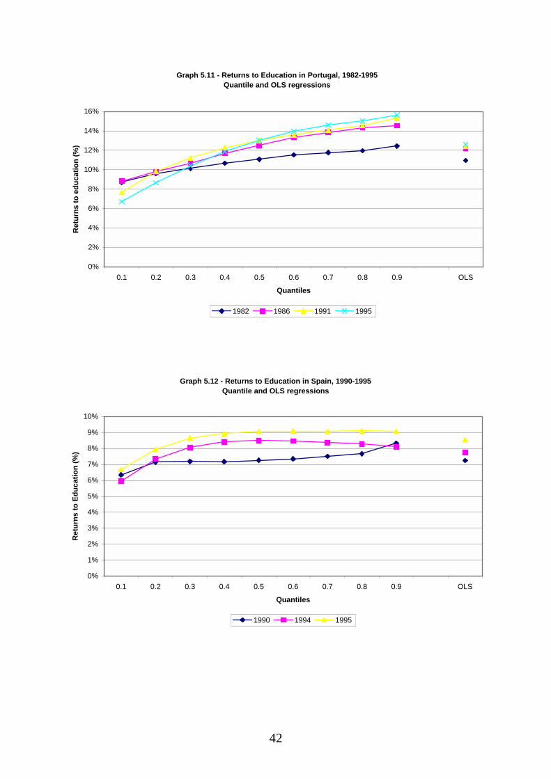
42

Graph 5.11 - Returns to Education in Portugal, 1982-1995 Quantile and OLS regressions

0%

2%

4%

6%

8%

10%

12%

14%

16%

0.1 0.2 0.3 0.4 0.5 0.6 0.7 0.8 0.9 OLS

Quantiles

Ret

urn

s to

ed

uca

tio

n (

%)

1982 1986 1991 1995

Graph 5.12 - Returns to Education in Spain, 1990-1995 Quantile and OLS regressions

0%

1%

2%

3%

4%

5%

6%

7%

8%

9%

10%

0.1 0.2 0.3 0.4 0.5 0.6 0.7 0.8 0.9 OLS

Quantiles

Ret

urn

s to

Ed

uca

tio

n (

%)

1990 1994 1995

43

Graph 5.13 - Returns to Education in Sweden, 1981-1991 Quantile and OLS regressions

0%

1%

2%

3%

4%

5%

6%

7%

0.1 0.2 0.3 0.4 0.5 0.6 0.7 0.8 0.9 OLS

Quantiles

Ret

urn

s to

Ed

uca

tio

n (

%)

1981 1991

Graph 5.14 - Returns to Education in Switzerland, 1992-1998Quantile and OLS regressions

0.0%

2.0%

4.0%

6.0%

8.0%

10.0%

12.0%

0.1 0.2 0.3 0.4 0.5 0.6 0.7 0.8 0.9 OLS

Quantiles

Ret

urn

s to

Ed

uca

tio

n (

%)

1992 1995 1998

44

Graph 5.15 - Returns to Education in the UK, 1980-1995Quantile and OLS regressions

0%

2%

4%

6%

8%

10%

12%

0.1 0.2 0.3 0.4 0.5 0.6 0.7 0.8 0.9 OLS

Deciles

Ret

urn

s to

Ed

uca

tio

n (

%)

1980 1985 1990 1995

45

Table 5.1 - Quantile regressions results (coefficients and SE's)

0,1 0,088 0,0048 0,080 0,0032 0,078 0,0047 0,070 0,0034

0,2 0,086 0,0030 0,086 0,0027 0,086 0,0029 0,075 0,0030

0,3 0,095 0,0023 0,088 0,0035 0,091 0,0029 0,082 0,0020

0,4 0,097 0,0035 0,093 0,0023 0,095 0,0020 0,087 0,0028

0,5 0,101 0,0034 0,095 0,0024 0,097 0,0022 0,091 0,0031

0,6 0,104 0,0039 0,098 0,0025 0,100 0,0022 0,098 0,0034

0,7 0,110 0,0050 0,102 0,0029 0,101 0,0031 0,106 0,0042

0,8 0,115 0,0042 0,103 0,0042 0,105 0,0030 0,113 0,0031

0,9 0,118 0,0047 0,114 0,0039 0,113 0,0049 0,120 0,0046

OLS 0,100 0,0019 0,095 0,0020 0,095 0,0023 0,093 0,0021

0,1 0,046 0,0021 0,041 0,0023 0,047 0,0023 0,061 0,0026

0,2 0,043 0,0021 0,040 0,0019 0,048 0,0018 0,062 0,0020

0,3 0,045 0,0017 0,042 0,0016 0,049 0,0017 0,061 0,0016

0,4 0,044 0,0016 0,044 0,0018 0,051 0,0021 0,061 0,0017

0,5 0,047 0,0015 0,047 0,0020 0,054 0,0021 0,061 0,0021

0,6 0,048 0,0023 0,050 0,0019 0,056 0,0023 0,065 0,0019

0,7 0,047 0,0022 0,054 0,0023 0,059 0,0027 0,067 0,0024

0,8 0,050 0,0031 0,057 0,0031 0,060 0,0032 0,069 0,0024

0,9 0,051 0,0049 0,064 0,0035 0,062 0,0043 0,069 0,0041

OLS 0,045 0,0020 0,051 0,0018 0,055 0,0019 0,064 0,0018

0,1 0,070 0,0061 0,083 0,0061 0,066 0,0067

0,2 0,083 0,0046 0,086 0,0033 0,083 0,0048

0,3 0,087 0,0042 0,086 0,0038 0,080 0,0052

0,4 0,090 0,0036 0,094 0,0043 0,081 0,0042

0,5 0,095 0,0040 0,097 0,0032 0,088 0,0045

0,6 0,097 0,0043 0,094 0,0047 0,087 0,0050

0,7 0,097 0,0047 0,093 0,0043 0,092 0,0048

0,8 0,096 0,0056 0,089 0,0056 0,092 0,0062

0,9 0,098 0,0082 0,094 0,0081 0,096 0,0096

OLS 0,091 0,0037 0,090 0,0035 0,086 0,0042

0,1 0,0680 0,00155 0,0549 0,00207 0,0588 0,00149 0,0571 0,00203

0,2 0,0789 0,00135 0,0678 0,00125 0,0675 0,00129 0,0652 0,00197

0,3 0,0855 0,00133 0,0759 0,00122 0,0734 0,00097 0,0682 0,00183

0,4 0,0929 0,00128 0,0794 0,00100 0,0763 0,00107 0,0728 0,00188

0,5 0,0968 0,00129 0,0827 0,00106 0,0786 0,00117 0,0755 0,00174

0,6 0,0997 0,00115 0,0850 0,00111 0,0804 0,00108 0,0809 0,00210

0,7 0,1021 0,00131 0,0886 0,00111 0,0828 0,00119 0,0825 0,00216

0,8 0,1025 0,00133 0,0919 0,00123 0,0835 0,00141 0,0840 0,00290

0,9 0,1005 0,00183 0,0938 0,00150 0,0835 0,00157 0,0890 0,00345

OLS 0,0866 0,00100 0,0723 0,00095 0,0710 0,00092 0,0733 0,00156

Denmark

Finland

France

1980 1985 1990

Austria

1981 1985 1989 1993

1995

1987 1989 1993

1970 1977 1985 1993

46

Table 5.1 - Quantile regressions results (cont.)

0.1 0.090 0.0043 0.096 0.0059 0.087 0.0044 0.082 0.0045

0.2 0.089 0.0030 0.092 0.0030 0.086 0.0038 0.077 0.0053

0.3 0.087 0.0034 0.090 0.0035 0.084 0.0035 0.073 0.0032

0.4 0.084 0.0033 0.085 0.0037 0.080 0.0042 0.074 0.0033

0.5 0.083 0.0036 0.080 0.0036 0.079 0.0047 0.076 0.0033

0.6 0.083 0.0035 0.082 0.0027 0.080 0.0030 0.078 0.0032

0.7 0.084 0.0024 0.084 0.0040 0.076 0.0034 0.077 0.0030

0.8 0.084 0.0044 0.090 0.0053 0.077 0.0059 0.075 0.0037

0.9 0.081 0.0057 0.092 0.0075 0.074 0.0034 0.072 0.0044

0.1 0.063 0.0031 0.049 0.0043 0.073 0.0072

0.2 0.058 0.0024 0.044 0.0032 0.063 0.0043

0.3 0.058 0.0022 0.047 0.0025 0.060 0.0041

0.4 0.058 0.0023 0.045 0.0023 0.059 0.0028

0.5 0.054 0.0024 0.044 0.0020 0.056 0.0027

0.6 0.052 0.0030 0.044 0.0020 0.056 0.0028

0.7 0.056 0.0036 0.045 0.0027 0.055 0.0029

0.8 0.057 0.0042 0.047 0.0034 0.053 0.0034

0.9 0.053 0.0050 0.047 0.0042 0.055 0.0047

OLS 0.057 0.0024 0.050 0.0027 0.063 0.0033

0.1 0.096 0.0089 0.075 0.0102

0.2 0.086 0.0083 0.085 0.0056

0.3 0.087 0.0066 0.087 0.0048

0.4 0.102 0.0049 0.089 0.0040

0.5 0.105 0.0060 0.099 0.0052

0.6 0.105 0.0057 0.098 0.0055

0.7 0.103 0.0055 0.100 0.0044

0.8 0.104 0.0073 0.102 0.0032

0.9 0.099 0.0087 0.099 0.0049

OLS 0.097 0.0053 0.086 0.0047

0.1 0.039 0.0052 0.043 0.0037 0.039 0.0021 0.065 0.0034

0.2 0.033 0.0035 0.036 0.0026 0.037 0.0017 0.063 0.0024

0.3 0.034 0.0018 0.037 0.0020 0.037 0.0014 0.057 0.0021

0.4 0.034 0.0025 0.035 0.0019 0.040 0.0016 0.057 0.0017

0.5 0.034 0.0018 0.036 0.0019 0.040 0.0018 0.056 0.0015

0.6 0.035 0.0078 0.035 0.0014 0.041 0.0018 0.057 0.0019

0.7 0.035 0.0017 0.037 0.0022 0.041 0.0014 0.061 0.0020

0.8 0.039 0.0022 0.041 0.0021 0.045 0.0020 0.065 0.0026

0.9 0.045 0.0036 0.042 0.0033 0.049 0.0027 0.068 0.0033

OLS 0.042 0.0025 0.042 0.0021 0.042 0.0013 0.062 0.0017

1974 1988

1989 1995

Germany

1991 1995

1987 1994

Ireland

1984 1986

1994

Greece

Italy

1980 1984

47

Table 5.1 - Quantile regressions results (cont.)

0.1 0.063 0.0006 0.046 0.0011 0.051 0.0014

0.2 0.071 0.0007 0.053 0.0008 0.054 0.0008

0.3 0.076 0.0008 0.055 0.0008 0.059 0.0008

0.4 0.078 0.0008 0.059 0.0009 0.061 0.0007

0.5 0.082 0.0008 0.062 0.0009 0.063 0.0007

0.6 0.085 0.0010 0.067 0.0011 0.066 0.0008

0.7 0.088 0.0009 0.070 0.0012 0.070 0.0008

0.8 0.088 0.0011 0.074 0.0014 0.074 0.0010

0.9 0.088 0.0013 0.078 0.0021 0.079 0.0013

OLS 0.083 0.0004 0.066 0.0008 0.068 0.0006

0.1 0.052 0.0049 0.035 0.0062 0.058 0.0070 0.053 0.0071

0.2 0.049 0.0033 0.040 0.0042 0.046 0.0043 0.048 0.0043

0.3 0.052 0.0031 0.042 0.0037 0.048 0.0031 0.051 0.0042

0.4 0.051 0.0034 0.045 0.0044 0.045 0.0028 0.049 0.0025

0.5 0.056 0.0032 0.046 0.0041 0.046 0.0028 0.056 0.0039

0.6 0.057 0.0032 0.051 0.0037 0.048 0.0036 0.065 0.0044

0.7 0.059 0.0037 0.056 0.0038 0.058 0.0043 0.069 0.0060

0.8 0.064 0.0037 0.052 0.0050 0.060 0.0039 0.070 0.0049

0.9 0.061 0.0064 0.051 0.0060 0.052 0.0071 0.073 0.0080

OLS 0.056 0.0030 0.045 0.0035 0.054 0.0035 0.059 0.0039

0.1 0.083 0.0012 0.085 0.0012 0.074 0.0009 0.065 0.0010

0.2 0.092 0.0010 0.093 0.0009 0.094 0.0008 0.083 0.0010

0.3 0.097 0.0009 0.101 0.0010 0.106 0.0009 0.099 0.0009

0.4 0.101 0.0009 0.110 0.0009 0.116 0.0009 0.112 0.0009

0.5 0.105 0.0010 0.118 0.0011 0.122 0.0009 0.122 0.0009

0.6 0.109 0.0011 0.125 0.0010 0.127 0.0009 0.131 0.0011

0.7 0.111 0.0011 0.130 0.0012 0.132 0.0011 0.136 0.0012

0.8 0.113 0.0013 0.134 0.0012 0.136 0.0013 0.140 0.0013

0.9 0.117 0.0016 0.136 0.0019 0.142 0.0017 0.145 0.0017

OLS 0.104 0.0009 0.115 0.0009 0.117 0.0009 0.119 0.0009

0.1 0.062 0.0013 0.058 0.0028 0.065 0.0004

0.2 0.069 0.0011 0.071 0.0030 0.076 0.0004

0.3 0.069 0.0012 0.077 0.0029 0.083 0.0004

0.4 0.069 0.0011 0.081 0.0032 0.086 0.0004

0.5 0.070 0.0009 0.082 0.0026 0.087 0.0004

0.6 0.071 0.0012 0.081 0.0032 0.087 0.0004

0.7 0.072 0.0013 0.080 0.0040 0.087 0.0004

0.8 0.074 0.0014 0.080 0.0042 0.087 0.0005

0.9 0.080 0.0019 0.078 0.0040 0.087 0.0006

OLS 0.070 0.0095 0.075 0.0024 0.082 0.0003

1979 1989 1996

Netherlands

Norway

1983 1987 1991 1995

Portugal

1982 1986 1991 1995

1990 1994 1995

Spain

48

Table 5.1 - Quantile regressions results (cont.)

0,1 0,032 0,0024 0,024 0,0027

0,2 0,035 0,0016 0,028 0,0021

0,3 0,037 0,0018 0,031 0,0022

0,4 0,040 0,0017 0,036 0,0023

0,5 0,044 0,0016 0,043 0,0026

0,6 0,047 0,0020 0,045 0,0025

0,7 0,051 0,0023 0,050 0,0029

0,8 0,059 0,0030 0,055 0,0036

0,9 0,063 0,0041 0,060 0,0044

OLS 0,046 0,0020 0,041 0,0022

0,1 0,079 0,0050 0,084 0,0036 0,061 0,0037

0,2 0,085 0,0033 0,084 0,0024 0,076 0,0030

0,3 0,092 0,0028 0,086 0,0022 0,081 0,0022

0,4 0,092 0,0029 0,090 0,0016 0,082 0,0025

0,5 0,092 0,0023 0,092 0,0014 0,084 0,0025

0,6 0,092 0,0025 0,094 0,0018 0,087 0,0023

0,7 0,095 0,0028 0,096 0,0016 0,090 0,0028

0,8 0,100 0,0025 0,100 0,0020 0,091 0,0030

0,9 0,102 0,0046 0,101 0,0026 0,097 0,0036

OLS 0,091 0,0026 0,090 0,0019 0,086 0,0024

0,1 0,024 0,0049 0,053 0,0054 0,055 0,0067 0,048 0,0070

0,2 0,039 0,0041 0,050 0,0046 0,060 0,0047 0,056 0,0056

0,3 0,051 0,0042 0,060 0,0041 0,067 0,0051 0,066 0,0053

0,4 0,056 0,0034 0,066 0,0036 0,070 0,0049 0,071 0,0047

0,5 0,061 0,0036 0,066 0,0046 0,072 0,0051 0,070 0,0042

0,6 0,058 0,0031 0,070 0,0034 0,072 0,0038 0,070 0,0036

0,7 0,062 0,0039 0,073 0,0040 0,069 0,0037 0,069 0,0040

0,8 0,071 0,0039 0,077 0,0051 0,082 0,0043 0,075 0,0049

0,9 0,071 0,0058 0,075 0,0047 0,087 0,0053 0,092 0,0060

OLS 0,065 0,0034 0,078 0,0038 0,083 0,0039 0,083 0,0041

United Kingdom

1980 1985 1990 1995

1981 1991

Sweden

1992 1995 1998

Switzerland

49

Table 5.2 - Summary of results

Country Years 1st dec. 9th dec. OLS

Austria 1981 9.2% 12.6% 10.5%1993 7.2% 12.8% 9.7%

Denmark 1980 4.7% 5.3% 4.6%1995 6.3% 7.1% 6.6%

Finland 1987 7.3% 10.3% 9.5%1993 6.8% 10.1% 8.9%

France 1977 5.6% 9.8% 7.5%1993 5.9% 9.3% 7.6%

Germany 1984 9.4% 8.4%1995 8.5% 7.5%

Greece 1974 6.5% 5.4% 5.8%1994 7.5% 5.6% 6.5%

Italy 1980 3.9% 4.6% 4.3%1995 6.7% 7.1% 6.4%

Ireland 1987 10.1% 10.4% 10.2%1994 7.8% 10.4% 8.9%

Netherlands 1979 6.5% 9.2% 8.6%1996 5.3% 8.3% 7.0%

Norway 1983 5.3% 6.3% 5.7%1995 5.5% 7.5% 6.0%

Portugal 1982 8.7% 12.4% 11.0%1995 6.7% 15.6% 12.6%

Spain 1990 6.4% 8.3% 7.2%1995 6.7% 9.1% 8.6%

Sweden 1981 3.2% 6.6% 4.7%1991 2.4% 6.2% 4.1%

Switzerland 1992 8.2% 10.7% 9.6%1998 6.3% 10.2% 9.0%

UK 1980 2.5% 7.4% 6.7%1995 4.9% 9.7% 8.6%

Means First Year 6.3% 8.5% 7.6%St. Dev. 2.3% 2.6% 2.3%

Coeff. Var. 0.36 0.31 0.31

Means Last year 6.1% 9.2% 7.9%St. Dev. 1.4% 2.7% 2.0%

Coeff. Var. 0.22 0.29 0.26

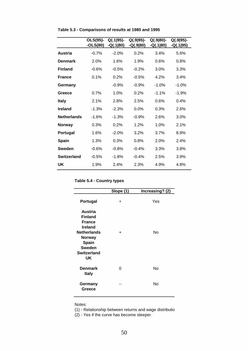
50

Table 5.3 - Comparisons of results at 1980 and 1995

OLS(95)- Q(.1|95)- Q(.9|95)- Q(.9|80)- Q(.9|95)--OLS(80) -Q(.1|80) -Q(.9|80) -Q(.1|80) -Q(.1|95)

Austria -0.7% -2.0% 0.2% 3.4% 5.6%

Denmark 2.0% 1.6% 1.9% 0.6% 0.8%

Finland -0.6% -0.5% -0.2% 3.0% 3.3%

France 0.1% 0.2% -0.5% 4.2% 3.4%

Germany -0.9% -0.9% -1.0% -1.0%

Greece 0.7% 1.0% 0.2% -1.1% -1.9%

Italy 2.1% 2.8% 2.5% 0.6% 0.4%

Ireland -1.3% -2.3% 0.0% 0.3% 2.6%

Netherlands -1.6% -1.3% -0.9% 2.6% 3.0%

Norway 0.3% 0.2% 1.2% 1.0% 2.1%

Portugal 1.6% -2.0% 3.2% 3.7% 8.9%

Spain 1.3% 0.3% 0.8% 2.0% 2.4%

Sweden -0.6% -0.8% -0.4% 3.3% 3.8%

Switzerland -0.5% -1.8% -0.4% 2.5% 3.9%

UK 1.9% 2.4% 2.3% 4.9% 4.8%

Table 5.4 - Country types

Slope (1) Increasing? (2)

Portugal + Yes

AustriaFinlandFranceIreland

Netherlands + NoNorwaySpain

SwedenSwitzerland

UK

Denmark 0 NoItaly

Germany -- NoGreece

Notes:(1) - Relationship between returns and wage distributio(2) - Yes if the curve has become steeper.

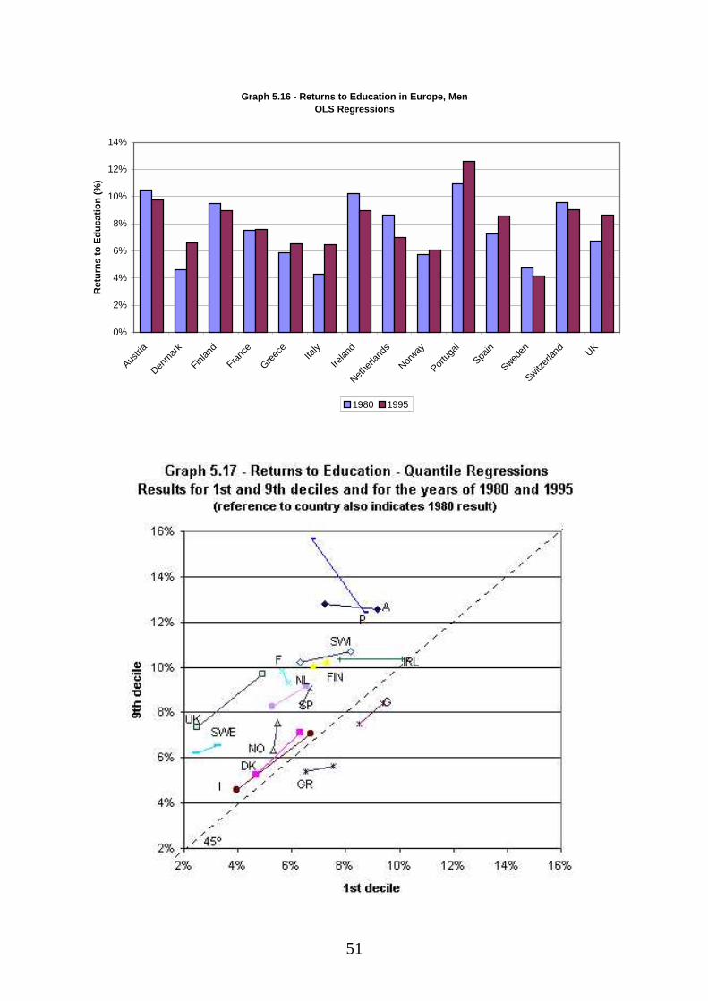
51

Graph 5.16 - Returns to Education in Europe, MenOLS Regressions

0%

2%

4%

6%

8%

10%

12%

14%

Austri

a

Denm

ark

Finlan

d

Franc

e

Greec

eIta

ly

Irelan

d

Nethe

rland

s

Norway

Portu

gal

Spain

Sweden

Switzer

land

UK

Ret

urn

s to

Ed

uca

tio

n (

%)

1980 1995

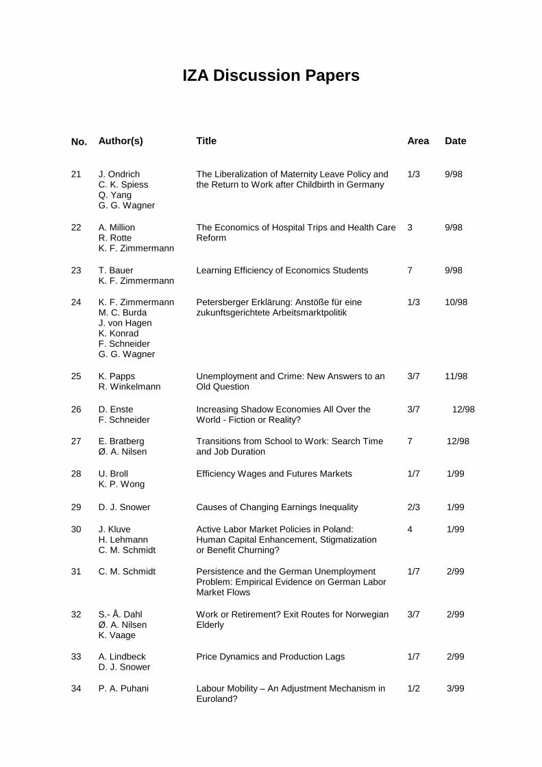
IZA Discussion Papers No.

Author(s)

Title

Area

Date

21

J. Ondrich C. K. Spiess Q. Yang G. G. Wagner

The Liberalization of Maternity Leave Policy and the Return to Work after Childbirth in Germany

1/3

9/98

22

A. Million R. Rotte K. F. Zimmermann

The Economics of Hospital Trips and Health Care Reform

3

9/98

23

T. Bauer K. F. Zimmermann

Learning Efficiency of Economics Students

7

9/98

24 K. F. Zimmermann M. C. Burda J. von Hagen K. Konrad F. Schneider G. G. Wagner

Petersberger Erklärung: Anstöße für eine zukunftsgerichtete Arbeitsmarktpolitik

1/3 10/98

25

K. Papps R. Winkelmann

Unemployment and Crime: New Answers to an Old Question

3/7

11/98

26 D. Enste

F. Schneider Increasing Shadow Economies All Over the World - Fiction or Reality?

3/7 12/98

27 E. Bratberg Ø. A. Nilsen

Transitions from School to Work: Search Time and Job Duration

7 12/98

28 U. Broll

K. P. Wong Efficiency Wages and Futures Markets

1/7 1/99

29 D. J. Snower Causes of Changing Earnings Inequality 2/3 1/99

30 J. Kluve

H. Lehmann C. M. Schmidt

Active Labor Market Policies in Poland: Human Capital Enhancement, Stigmatization or Benefit Churning?

4 1/99

31

C. M. Schmidt

Persistence and the German Unemployment Problem: Empirical Evidence on German Labor Market Flows

1/7 2/99

32 S.- Å. Dahl

Ø. A. Nilsen K. Vaage

Work or Retirement? Exit Routes for Norwegian Elderly

3/7 2/99

33 A. Lindbeck D. J. Snower

Price Dynamics and Production Lags 1/7 2/99

34 P. A. Puhani Labour Mobility – An Adjustment Mechanism in Euroland?

1/2 3/99

35 D. A. Jaeger A. Huff Stevens

Is Job Stability in the United States Falling? Reconciling Trends in the Current Population Survey and Panel Study of Income Dynamics

1 3/99

36 C. Lauer The Effects of European Economic and Monetary Union on Wage Behaviour

1/2 3/99

37 H. S. Buscher

C. Müller Exchange Rate Volatility Effects on the German Labour Market: A Survey of Recent Results and Extensions

1/2 3/99

38 M. E. Ward

P. J. Sloane

Job Satisfaction within the Scottish Academic Profession

7 4/99

39 A. Lindbeck D. J. Snower

Multi-Task Learning and the Reorganization of Work

1/5 4/99

40 S. M. Golder T. Straubhaar

Empirical Findings on the Swiss Migration Experience

1 4/99

41 J. M. Orszag Anatomy of Policy Complementarities 3/7 5/99 D. J. Snower

42 D. S. Hamermesh The Changing Distribution of Job Satisfaction

7 5/99

43 C. Belzil J. Hansen

Household Characteristics, Ability and Education: Evidence from a Dynamic Expected Utility Model

7 5/99

44 D. N. F. Bell R. A. Hart

Overtime Working in an Unregulated Labour Market

1 6/99

45 R. A. Hart

J. R. Malley On the Cyclicality and Stability of Real Earnings 1 6/99

46 R. Rotte

M. Vogler The Effects of Development on Migration: Theoretical Issues and New Empirical Evidence

2 6/99

47 R. A. Hart

F. Ritchie Tenure-based Wage Setting

1/7 7/99

48 T. Bauer K. F. Zimmermann

Overtime Work and Overtime Compensation in Germany

1 7/99

49 H. P. Grüner Unemployment and Labor-Market Reform: A Contract Theoretic Approach

1/3 7/99

50 K. F. Zimmermann Ethnic German Migration After 1989 – Balance and Perspectives

1 8/99

51 A. Barrett

P. J. O’Connell Does Training Generally Work? The Returns to In-Company Training

7 8/99

52 J. Mayer R. T. Riphahn

Fertility Assimilation of Immigrants: Evidence from Count Data Models

3 8/99

53 J. Hartog

P. T. Pereira J. A. C. Vieira

Inter-industry Wage Dispersion in Portugal: high but falling

7 8/99

54 M. Lofstrom

Labor Market Assimilation and the Self-Employment Decision of Immigrant Entrepreneurs

1 8/99

55 L. Goerke

Value-added Tax versus Social Security Contributions

3 8/99

56 A. Lindbeck D. J. Snower

Centralized Bargaining and Reorganized Work: Are they compatible?

1/5 9/99

57 I. N. Gang K. F. Zimmermann

Is Child like Parent? Educational Attainment and Ethnic Origin

1 9/99

58 T. Bauer

K. F. Zimmermann Occupational Mobility of Ethnic Migrants 1 9/99

59 D. J. DeVoretz

S. A. Laryea Canadian Immigration Experience: Any Lessons for Europe?

1/2/3 9/99

60 C. Belzil

J. Hansen Subjective Discount Rates, Intergenerational Transfers and the Return to Schooling

7 10/99

61 R. Winkelmann Immigration: The New Zealand Experience 7 10/99 62 A. Thalmaier Bestimmungsgründe von Fehlzeiten: Welche

Rolle spielt die Arbeitslosigkeit? 3 10/99

63 M. Ward Your Everyday, Average Academic 5 10/99

64 M. Ward Salary and the Gender Salary Gap in the

Academic Profession 5 10/99

65 H. Lehmann

J. Wadsworth A. Acquisti

Grime and Punishment: Job Insecurity and Wage Arrears in the Russian Federation

4 10/99

66 E. J. Bird

H. Kayser J. R. Frick G. G. Wagner

The Immigrant Welfare Effect: Take-Up or Eligibility?

3 10/99

67 R. T. Riphahn

A. Thalmaier Behavioral Effects of Probation Periods: An Analysis of Worker Absenteeism

1/3 10/99

68 B. Dietz

Ethnic German Immigration from Eastern Europe and the former Soviet Union to Germany: the Effects of Migrant Networks

1 11/99

69 M.-S. Yun

Generalized Selection Bias and the Decomposition of Wage Differentials

7 11/99

70 I. N. Gang F.L. Rivera-Batiz

Immigrants and Unemployment in the European Community

1 11/99

71 L. Goerke The Wedge

3 11/99

72 J. Fersterer R. Winter-Ebmer

Are Austrian Returns to Education Falling Over Time?

7 11/99

73 G. S. Epstein S. Nitzan

The Endogenous Determination of Minimum Wage

3 11/99

74 M. Kräkel Strategic Mismatches in Competing Teams

7 12/99

75 B. Henry M. Karanassou D. J. Snower

Adjustment Dynamics and the Natural Rate: An Account of UK Unemployment

1 12/99

76 G. Brunello M. Giannini

Selective Schools

7 12/99

77 C. M. Schmidt Knowing What Works: The Case for Rigorous Program Evaluation

6 12/99

78 J. Hansen R. Wahlberg

Endogenous Schooling and the Distribution of the Gender Wage Gap

7 12/99

79 J. S. Earle Z. Sakova

Entrepreneurship from Scratch: Lessons on the Entry Decision into Self-Employment from Transition Economies

4 12/99

80 J. C. van Ours J. Veenman

The Netherlands: Old Emigrants – Young Immigrant Country

1 12/99

81 T. J. Hatton S. Wheatley Price

Migration, Migrants and Policy in the United Kingdom

1 12/99

82 K. A. Konrad Privacy, time consistent optimal labor income taxation and education policy

3 12/99

83 R. Euwals Female Labour Supply, Flexibility of Working Hours, and Job Mobility in the Netherlands

1 12/99

84 C. M. Schmidt The Heterogeneity and Cyclical Sensitivity of Unemployment: An Exploration of German Labor Market Flows

1 12/99

85 S. Pudney M. A. Shields

Gender and Racial Discrimination in Pay and Promotion for NHS Nurses

5/6 12/99

86 J.P. Haisken-DeNew C. M. Schmidt

Money for Nothing and Your Chips for Free? The Anatomy of the PC Wage Differential

5/7 12/99

87 T. K. Bauer Educational Mismatch and Wages in Germany

7 12/99

88 O. Bover P. Velilla

Migration in Spain: Historical Background and Current Trends

1 12/99

89 S. Neuman Aliyah to Israel: Immigration under Conditions of Adversity

1 12/99

90 H. Lehmann J. Wadsworth

Tenures that Shook the World: Worker Turnover in Russia, Poland and Britain

4 12/99

91 M. Lechner Identification and Estimation of Causal Effects of Multiple Treatments Under the Conditional Independence Assumption

6 12/99

92 R. E. Wright The Rate of Return to Private Schooling

7 12/99

93 M. Lechner An Evaluation of Public-Sector-Sponsored Continuous Vocational Training Programs in East Germany

6 12/99

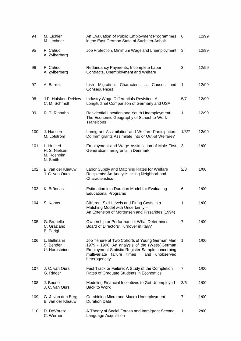
94 M. Eichler

M. Lechner An Evaluation of Public Employment Programmes in the East German State of Sachsen-Anhalt

6 12/99

95 P. Cahuc A. Zylberberg

Job Protection, Minimum Wage and Unemployment 3 12/99

96 P. Cahuc

A. Zylberberg Redundancy Payments, Incomplete Labor Contracts, Unemployment and Welfare

3 12/99

97 A. Barrett Irish Migration: Characteristics, Causes and

Consequences

1 12/99

98 J.P. Haisken-DeNew C. M. Schmidt

Industry Wage Differentials Revisited: A Longitudinal Comparison of Germany and USA

5/7 12/99

99 R. T. Riphahn Residential Location and Youth Unemployment: The Economic Geography of School-to-Work-Transitions

1 12/99

100 J. Hansen M. Lofstrom

Immigrant Assimilation and Welfare Participation: Do Immigrants Assimilate Into or Out-of Welfare?

1/3/7 12/99

101 L. Husted H. S. Nielsen M. Rosholm N. Smith

Employment and Wage Assimilation of Male First Generation Immigrants in Denmark

3 1/00

102 B. van der Klaauw J. C. van Ours

Labor Supply and Matching Rates for Welfare Recipients: An Analysis Using Neighborhood Characteristics

2/3 1/00

103 K. Brännäs Estimation in a Duration Model for Evaluating

Educational Programs

6 1/00

104 S. Kohns Different Skill Levels and Firing Costs in a Matching Model with Uncertainty – An Extension of Mortensen and Pissarides (1994)

1 1/00

105 G. Brunello C. Graziano B. Parigi

Ownership or Performance: What Determines Board of Directors' Turnover in Italy?

7 1/00

106 L. Bellmann S. Bender U. Hornsteiner

Job Tenure of Two Cohorts of Young German Men 1979 - 1990: An analysis of the (West-)German Employment Statistic Register Sample concerning multivariate failure times and unobserved heterogeneity

1 1/00

107 J. C. van Ours G. Ridder

Fast Track or Failure: A Study of the Completion Rates of Graduate Students in Economics

7 1/00

108 J. Boone J. C. van Ours

Modeling Financial Incentives to Get Unemployed Back to Work

3/6 1/00

109 G. J. van den Berg B. van der Klaauw

Combining Micro and Macro Unemployment Duration Data

7 1/00

110 D. DeVoretz C. Werner

A Theory of Social Forces and Immigrant Second Language Acquisition

1 2/00

111 V. Sorm K. Terrell

Sectoral Restructuring and Labor Mobility: A Comparative Look at the Czech Republic

1/4 2/00

112 L. Bellmann T. Schank

Innovations, Wages and Demand for Heterogeneous Labour: New Evidence from a Matched Employer-Employee Data-Set

5 2/00

113

R. Euwals

Do Mandatory Pensions Decrease Household Savings? Evidence for the Netherlands

7 2/00

114 G. Brunello

A. Medio An Explanation of International Differences in Education and Workplace Training

7 2/00

115 A. Cigno

F. C. Rosati Why do Indian Children Work, and is it Bad for Them?

7 2/00

116 C. Belzil Unemployment Insurance and Subsequent Job Duration: Job Matching vs. Unobserved Heterogeneity

7 2/00

117

S. Bender A. Haas C. Klose

IAB Employment Subsample 1975-1995. Opportunities for Analysis Provided by the Anonymised Subsample

7 2/00

118 M. A. Shields

M. E. Ward Improving Nurse Retention in the British National Health Service: The Impact of Job Satisfaction on Intentions to Quit

5 2/00

119 A. Lindbeck D. J. Snower

The Division of Labor and the Market for Organizations

5 2/00

120 P. T. Pereira P. S. Martins

Does Education Reduce Wage Inequality? Quantile Regressions Evidence from Fifteen European Countries

5/7 2/00

An updated list of IZA Discussion Papers is available on the center‘s homepage www.iza.org.