Working Paper 12-09 Departamento de Economía Economic Series Universidad Carlos III de Madrid January, 2012 Calle Madrid, 126 28903 Getafe (Spain) Fax (34) 916249875

Unemployment Risk and Wage Differentials*

ROBERTO PINHEIRO† AND LUDO VISSCHERS‡

Abstract

Workers in less secure jobs are often paid less than identical-looking workers in more secure jobs. We show that this lack of compensating differentials for unemployment risk can arise in equilibrium when all workers are identical, and firms differ, but do so only in offered job security (the probability that the worker is not sent into unemployment). In a setting where workers search on and off the job, wages paid increase with job security for at least all firms in the risky tail of the distribution of firm-level unemployment risk. As a result, unemployment spells become persistent for low-wage and unemployed workers, a seeming pattern of ‘unemployment scarring’, that is created entirely by firm heterogeneity alone. Higher in the wage distribution, workers can take wage cuts to move to more stable employment.

Keywords: Layoff Rates, Unemployment risk, Wage Differentials, Unemployment Scarring JEL Codes : J31, J63

* We are grateful to numerous colleagues for insightful comments, and to Robert Kirkby for excellent research assistance. We also benefitted from the

feedback of several seminar audiences. The comments of 2 anonymous referees and the editor helped us improve this paper greatly. Naturally, all remaining errors are our own. Visschers acknowledges the support of Simon Fraser University’s President’s Research Gr ant, UC3M’s Instituto de Economí a; the Spanish Ministry of Science and Innovation, Grant 2011/00049/001, a grant from the Bank of Spain’s Programa de Investigación de Excelencia, and the Juan de la Cierva Fellowship. This paper was written in part while the second author was at Simon Fraser University.

† University of Colorado, Roberto(dot)Pinheiro(at)colorado(dot)edu.

‡ Department of Economics, U. Carlos III Madrid, lvissche(at)eco(dot)uc3m(dot)es

1 Introduction

When a transition into unemployment inflicts a loss on the worker, a competitive labor market requires a higherrisk of unemployment to be compensated by a higher wage. However, empirically, at the firm level the relationbetween job security - the probability of not becoming unemployed - and wages, seems to be positive or at theleast not significantly different from zero.1 For example, after controlling for worker and firm characteristicsincluding firm profit levels and firm exit probabilities, Mayo and Murray (1991), and Arai and Heyman (2001)find a positive correlation between job security and wages.2

The lack of compensating wages is even more puzzling, once it is observed that transitions to unemploy-ment also raise the prospect of shortened employment spells in the future. A job loss increases the probabilityof future job losses (e.g. Stevens 1997, Kletzer 1998). Such a reduction in subsequent employment durationsis responsible for a significant part of the cost of a transition into unemployment (Eliason and Storrie 2006,Böheim and Taylor 2002, Arulampalam et al. 2000). For displaced workers of a given quality, commonly, newjobs come with lower wages, and simultaneously with a higher risk of renewed unemployment (Cappellari andJenkins 2008, Uhlendorf 2006, Stewart 2007). These observations are in line with the absence of compensatingwage differentials at the firm level.

In addition, job security is partially related to observable and unobservable characteristics of the firmsoffering such positions. For example, larger firms tend to offer more secure jobs ( Morrissette 2004, Winter-Ebmer 1995, 2001). Escape from a sequence of low-pay and no-pay spells can occur when the same workeris lucky enough to land a high-wage job (Stewart 2007). In regression analyses of linked employer-employeedata Holzer, Lane and Vilhuber (2004) and Andersson, Holzer and Lane (2005) find that this higher-wage,more stable, employment appears to be concentrated in a subset of ‘good’ firms, i.e. firms with a high firmfixed effect. These firms are typically also larger.

We propose an equilibrium theory that is consistent with (i) the lack of compensating wage differentials,(ii) a pattern of ‘unemployment scarring’ through both repeated unemployment spells and lower wages, and(iii) the suggested importance of firm heterogeneity in shaping these. In our model, we follow Burdett andMortensen (1998), henceforth referred to as BM, and introduce search frictions and on-the-job search into anotherwise competitive setting. Our sole deviation from the BM setup, is that firms differ in the job security theyprovide, and not, for example, in the productivity of their workers. In this framework, even though workersask for a risk premium to stay at a risky job, fully compensating wage differentials are not offered in the labormarket equilibrium. Because of a shorter expected match duration, and a higher cost of offering the worker thesame life-time utility value, firms that offer only low job security have no incentive to compete with more solidfirms to keep workers for the long term. It then follows that workers move only from firms that offer risky jobs

1The literature testing for the relationship between job security at the firm level and wages is remarkably small. We know moreabout compensation for risk at different levels: for example, at the industry level the picture of compensating wage differentials isambiguous, with some evidence in favor of it (Abowd and Aschenfelter 1981 e.g.). Moretti (2000) found evidence that seasonal workearns a premium versus year-around work. However, patterns at industry level are not necessarily informative about what occurs atthe firm level. In this paper, we argue that search frictions, working between firms and workers within e.g. industries and occupations,can result in interesting non-linearities and interactions for the wage - unemployment risk relationship.

2When firm profit levels or firm exit probabilities are not controlled for, this relationship becomes even stronger, as wages and firmfailure probabilities are also negatively correlated, see for example Blanchflower (1991) and Carneiro and Portugal (2006)

2

to firms that offer safe jobs. The model then naturally produces an aggregate hazard rate for transitions intounemployment declining with time, whereas in the BM model the rate is counterfactually constant.

The value of more job security is low in jobs where the lifetime expected utility is only slightly higher thanthe value of unemployment. As a result, in these jobs, not only do the expected values of employment increasein job security, but the actual wages themselves increase in job security – a strong failure of compensatingdifferentials. This comes about because at the bottom of the wage distribution, even with different levels ofjob security, different types of firms are still in considerable wage competition with each other.3 We are ableto show that the increasing relationship between job security and wages extends at least to the entire ‘risky’tail of the firm distribution (i.e. the tail of the distribution with those firms that offer the lowest job security).

On the other hand, higher up in the equilibrium wage distribution, workers value job security more, andcould accept wage cuts to move to safer firms, and thus the model is consistent with wage cuts in job-to-jobtransitions, documented for example by Postel-Vinay and Robin (2002). We show that the extent to which thishappens depends also on the degree of competition on the firms’ side of the market: loosely, wage cuts canoccur if, increasing with job security, there is a decreasing amount of firms with a similar extent of job securitycompeting for the same workers.4

By themselves, the apparent lack of compensating differentials and unemployment scarring can also beexplained by worker heterogeneity and learning about match quality as well. It is possible to distinguish ourmechanism from those alternatives by looking at further implications of these theories. We discuss this in detailin the last section. These different implications could then naturally be used to measure how much worker,match, and firm heterogeneity each contribute to the risk of job loss. At this stage, it’s worth reiterating thatmany of the empirical papers mentioned above have attempted to control for worker heterogeneity, and stillfound significant scarring effects, suggesting a significant role for alternative mechanisms.

In short, our model is an equilibrium model of the wage ladder, where, endogenously, the lowest rungsof the wage ladder are especially slippery. It can explain the lack of compensating differentials, ‘genuine’unemployment scarring, and the correlation with firm identities and characteristics. The model also producesa negative correlation between firm size and unemployment risk that operates through the same channel asin the BM model. The literature has hitherto largely ignored the effects of heterogeneity in the firm-specificcomponent of job security by itself (and not related to imminent plant closures) in shaping patterns of lowfuture wages and repeated job loss for those currently unemployed.5 If firm heterogeneity is a leading factorbehind these patterns, there are also clear policy implications. First, as it creates persistence in bad labor mar-

3Hwang, Mortensen and Reed (1998) study a labor market with on-the-job search where firms pay wages and provide job amenities.In their model the valuation of the amenity is constant and given, in our model the valuation of job security depends endogenously onthe firm’s wage and the entire wage distribution. Job security also differs because it is strongly complementary with wages: the lowestwages will necessarily be at the riskiest firms, independently of, e.g., the firm distribution.

4In the most straightforward case, where a finite number of types exist, and hence, some firms do not face competition from verysimilar types on the upside and downside, wage cuts will occur, independently of parameter values, as shown in Pinheiro and Visschers2009.

5Some have argued that heterogeneity on both sides of the market, with low-quality, unstable workers sorting into unstable firms,can explain the lack of compensating differentials (Evans and Leighton 1989, for example). These arguments seem to imply thatworker heterogeneity is still a necessary condition to create patterns of wages increasing in job security. This paper argues, on thecontrary, that firm heterogeneity alone can generate these patterns.

3

ket outcomes, it would likely increase the inferred risk that a typical worker faces in the labor market. Then,incorporating that the first rungs of the wage ladder are more slippery has further implications for the consump-tion/savings tradeoff of workers who have just become unemployed, and, ex ante, for employed workers whoface differing risks of becoming unemployed, with more dire consequences if they do fall off the job ladder,into unemployment.6 Secondly, it could mean that policies attempting to diminish the heterogeneity, both inworkers’ initial conditions, for example by investing in education, and the conditions later in life, to make upfor perceived human capital loss while unemployed, might not be as effective as has sometimes been assumed.From a negative correlation between wages and job insecurity, and more importantly, a perceived joint causeof both of these on the worker’s side, it is tempting to conclude that increasing a worker’s earnings capacitywould also increase his or her job security in subsequent jobs. However, this gain in job security might not berealized when its cause lies not with the worker, but –without being affected by worker-centered policies– onthe firm’s side.

2 Model

A measure 1 of risk-neutral firms and a measure m of risk-neutral workers live forever, and discount the futureat rate r. All firms produce an identical amount of output p per worker, but differ in the probability δ withwhich they send workers back into unemployment. We index firms by this probability, and will refer to ahigh-δ firm as a “risky firm”, and a low-δ firm as a “solid firm”. The distribution function of firm types isH(δ); this distribution can contain mass points. Apart from the differences in layoff risk δ, the setup furtherfollows Burdett and Mortensen (1998). The labor market is subject to search frictions: unemployed workersreceive a single job offer at rate λ0, employed workers at rate λ1. This offer can be accepted or rejected on thespot, no recall of a rejected offer is possible. An offer is a wage w to be paid by the firm as long as the matchlasts; unemployed workers receive b each period they are without a job. Firms are committed to the postedwage, which has to be the same for every worker in the firm, and are able to hire everyone who accepts theiroffer. They maximize steady state profits.

2.1 Worker’s Problem and Risk-Equivalent Wages

Consider that firms with layoff risk δ post according to a symmetric, possibly pure, strategy with cdf F (w|δ).We can express the value functions of workers as follows: for unemployed workers

rV0 = b+ λ0

∫ ∫max{V (w, δ)− V0, 0}dF (w|δ)dH(δ). (1)

Similarly, for employed workers

rV (w, δ) = w + λ1

∫ ∫max{V (w′, δ′)− V (w, δ), 0}dF (w′|δ′)dH(δ′) + δ(V0 − V (w, δ)) (2)

6See Lise (2011) for a model linking the climbs of the wage ladder through on-the-job search, and the drops from the wage ladder,to consumption and savings decisions. In his model, following BM, the risk of dropping from the ladder is constant across workersand jobs.

4

The optimal policy is a reservation value policy, and by the monotonicity of value function (2) in w whilekeeping δ fixed, and vice versa, it follows that, given a current (w, δ) there is a reservation wage functionw′ = wr(δ′;w, δ) such that each (w′, δ′) yields a lifetime expected value equal to the value of employmentat wage w in a firm with layoff probability δ. This function can be derived directly from the above equations,given that V (wr(δ′;w, δ), δ′) = V (w, δ). When taking the wage at the most solid firm as the reference wage,we can define

w∗(ws, δ)def= wr(δ, ws, δ) = ws + (δ − δ)(V (ws, δ)− V0), (3)

which implies that the difference between a wage at a firm with unemployment risk δ and the equally preferredwage at the most solid firm δ is precisely the per-period expected loss due to decreased job security in themore risky firm. In case of this indifference, we refer to the latter as solid-firm equivalent wage. Below, todistinguish solid-firm equivalent wages from actual wages paid, we superscript the former, ws, while star thelatter, w∗, when necessary.

We can find the function that links wages at firms with unemployment risk δ with their solid-firm equivalentwage as the solution to a partial differential equation.

Lemma 1. The reservation (equivalent) wage function w∗(ws, δ) is the solution to the following partial dif-ferential equation

∂w∗(ws, δ)

∂ws=r + δ + λ1(1−

∫F (w∗(ws, δ′)|δ′)dH(δ′) )

r + δ + λ1(1−∫F (w∗(ws, δ′)|δ′)dH(δ′) )

(4)

∂w∗(ws, δ)

∂δ=w∗(ws, δ)− ws

δ − δ, (5)

with initial conditions for every δ,

w∗(R0, δ) = R0, where R0 solves V (R0, δ) = V0. (6)

We have relegated all proofs to the appendix. Now, with the wage equivalence function in hand, we canmap all wages into their solid-firm equivalent wage, and construct its cdf.

Corollary 1: DefineF (ws) =∫F (w∗(ws, δ′)|δ′)dH(δ′). Then the left and right derivativesF ′−(ws), F ′+(ws)

exist a.e., and so do the second right/left derivatives of the equivalent wage function, with

∂2+w∗

∂ws∂ws=

λ1(δ − δ)F ′−(ws))

(r + λ1(1− F (ws)) + δ)2≥ 0,

∂2w∗

∂ws∂δ=

1

(r + λ1(1− F (ws)) + δ)> 0, (7)

The solution to the PDE allows us to compare wages, and construct a wage offer distribution in termsof solid-firm equivalent wages. Initial conditions (6) follow directly from (3), but are interesting in terms ofeconomics as well: they state that at the reservation wage out of unemployment, the probability of becomingunemployed again is irrelevant.7 Job security is only valued above the reservation wage for the unemployed.Intuitively, if one is indifferent between being in state A or B, whether one transits from one to the other, andthus also how frequently, is irrelevant. Moreover, job security differs from e.g. standard differences in firms’

7See also Burdett and Mortensen 1980.

5

productivities (as discussed in BM, or Bontemps et al. 1999) because value of job security is endogenous,and it also depends on the distribution of wages offered in equilibrium. To be indifferent at a wage above R0,more risky wage offers naturally should come with higher wages. However, the increase in wages requiredfor risky firms is increasing more than proportionally with the increase in the wage offered by the solid firm,as wages get further away from the reservation wage. Put otherwise, there is an endogenous complementaritybetween job safety and wage levels, evidenced by the positive cross derivative in Corollary 1: safety becomesincreasingly valuable at higher wages (and conversely, high wages are more valuable in safer jobs).

2.2 The Firm’s Problem and Labor Market Equilibrium

The firm’s profit can be split up in two components: (i) the wage it pays per worker, leaving an instantaneousper-worker profit flow p−w∗(ws, δ), and (ii) the steady state amount of workers the firm has l(ws, δ). Takingas given the firm’s δ, there is a clear trade-off between the two components: higher wages mean less profit perworker at a given moment – but a worker will stay longer at the firm, and moreover, more potential workersfrom other firms will accept offers from the firm, resulting in a larger firm size l(ws, δ). Let G(ws, δ) be thejoint distribution of solid-firm equivalent wages and unemployment risks. Steady state dictates that the massof workers with ws′ ≤ ws, and δ ≤ δ′ is unchanging; with standard random matching (see Podczeck andPuzzello 2011), the dynamic evolution of the measure of workers can be expressed as8∫

δ′≤δ,R0≤ws′≤ws

(δ′ + λ1

∫ws>ws

dF (ws, δ) + λ1

∫δ>δ,

ws≥ws>ws′dF (ws, δ)

)dG(ws′, δ′)(m− u) =∫

δ′≤δ,R0≤ws′≤ws

(λ0u+ λ1

∫δ>δ,ws<ws′

dG(ws, δ)(m− u)

)dF (ws′, δ′) (8)

where the LHS is the outflow consisting of (in order) the outflow to unemployment (δ′), to firms with a higherwage ws > ws, and to firms with different δ′ > δ that offer wages higher than the current wage, but weaklylower than ws; the inflow, on the RHS, comes from unemployment or from firms with δ′ > δ, with lowerequivalent wages. Steady state dictates that inflow equals outflow; using (8) we can derive the firm size. Itfollows that G(ws, δ) is absolutely continuous with respect to F (ws, δ): if a subset A ∈ R2 has probability∫A dF (w, δ) equal to zero, then the LHS of (8), adapted to integrate only over the set A, equals zero; sinceδ > 0,∀δ, it must be that

∫A dG(w, δ) = 0 as well. Then, by the Radon-Nikodym theorem, a function l(ws, δ)

exists such that (m− u)G(ws, δ) =∫ wsws

∫ δδ l(w

s, δ)dF (ws, δ); Roughly, l(ws, δ) corresponds to the measureof workers divided by the measure of firms, as both get very small, and we take this as the firm size.

Lemma 2. The size of a firm posting a wage of which the equivalent wage is ws, only depends on aggregateequivalent-wage distributions F (ws) and G(ws), and the firm’s own δ,

l(ws, δ) =λ0u+ λ1G

−(ws)(m− u)

λ1(1− F+(ws)) + δ, (9)

where G−(ws) =∫ws′<ws dG(ws′, δ′), F+(ws) =

∫ws′≤ws dF (ws′, δ′). (Note, these are integrated over the

entire set of δ).

8Note that, since mass can be concentrated at a single (w, δ), we are explicit whether the boundaries are included.

6

Likewise for unemployment,

λ0u

∫ws≥R0

dF (ws, δ) =

∫δdG(ws, δ) (10)

The size of a firm will be affected by both the (equivalent) wage and its own unemployment risk. Thisstands in contrast to BM and Bontemps et al., who allow many sources of heterogeneity on the firm andworker side, but keep the property that the firm size only depends on the wage. As a direct consequence ofthe dependence of firm size on (ws, δ), the distribution function of workers G(ws) =

∫w≤ws l(w, δ)dF (w, δ),

depends on the distribution of H(δ) directly –it affects the inflows into unemployment–, as well as indirectly,through the equilibrium wage strategies for a given type. In particular, outflows of workers into unemploymentare higher when high-δ firms dominate the lower part of the wage distribution, which makes the mass ofemployed workers who are willing to move to a firm with equivalent wage ws smaller (assuming inflows fromunemployment are the same); this, in turn will affect wage strategies of firms. In equilibrium, we have to takethese dependencies into account.

To return to the firm’s optimization, a firm with layoff rate δ choosesws to maximize (p−w∗(ws, δ))l(ws, δ).Combining lemma 1 and lemma 2, we can derive that wages will not be compensating fully for the employmentrisk

Proposition 1 (Ranking Property). Suppose two firms with layoff risk δl, δh such that δl < δh offer profitmaximizing equivalent wages wsl and wsh. Then, we must have wsl ≥ wsh.

Proposition 1 is proved without reference to the shape of H(δ), and therefore holds also whether it is adiscrete, continuous, or a mixture distribution. Intuitively, the gain of posting a higher equivalent wage islarger for more solid firms, because (i) the increase in the actual wage needed is lower, i.e. the marginal costof an equivalent-wage increase is lower for the solid firm, and (ii) the increase in the steady state number ofworkers is higher, i.e. the marginal benefit of an equivalent-wage increase is higher. Each of the two forcesby themselves would already yield the result of proposition 1. Overall, it means that safer firms have an ad-vantage offering higher equivalent wages, and hence higher values of employment. However, we cannot makeinferences yet about the actual wages posted; for this we have to study the equilibrium and its implicationsmore deeply.

Definition 1. The steady state equilibrium in this labor market consists of distributions F (w|δ), F (ws|δ),G(ws, δ), F (ws), G(ws); an unemployment rate u; a reservation function w∗(ws, δ) for employed workers,and a reservation wage R0 for unemployed workers, such that

1. workers’ utility maximization: acceptance decisions w∗(ws, δ), R0 are optimal, given F (w|δ) andH(δ), and derived from (4)-(6)

2. Firms’ profit maximization: given F (ws), G(ws), for each δ, ∃π such that ∀ ws ∈ supp F (ws|δ), itholds that π = (p− w∗(ws, δ))l(ws, δ) and ∀ ws /∈ supp F (ws|δ), π ≥ (p− w∗(ws, δ))l(ws, δ)

3. steady state distributions follow from individual decisions aggregated up: F (ws|δ) is derived fromF (w|δ) andH(δ) usingw∗(ws, δ), whileG(ws, δ), and u follow from the steady state labor market flowaccounting in (8)-(10), F (ws) andG(ws) follow from

∫ ∫w≤ws dF

s(ws|δ)dH(δ), and∫w≤ws dG(ws, δ).

7

Adapting the proofs in BM and Bontemps et al. to incorporate the heterogeneity in δ, we can show thatF (ws) is a continuous, strictly increasing distribution function, and so is G(ws). The intuition for this alsofollows the aforementioned papers: mass points in the distribution of offered wages or intermediate intervalswhere no firms offer wages, allow discrete gains in firm size or profit per worker, while the costs of suchdeviation can be made arbitrarily small.

Proposition 2. In equilibrium, we can derive the following about derived distribution F (ws): (i) The supportof the distribution of equivalent wages ws offered in equilibrium is a connected set, (ii) there are no masspoints in F (ws), (iii) the lowest wage offered is R0, i.e. F (R0) = 0. Properties (i)-(iii) likewise hold forG(ws) derived from F (ws) and (8).

Combining proposition 1 and proposition 2, the conditional distribution function F−1(δ|ws) has all prob-ability mass concentrated at a unique δ. Conversely, if H(δ) has a continuous probability density, it alsofollows that each δ posts a unique equivalent wage. Neither implies that an actual wage w∗ is offered by atmost one δ-type of firm: overlaps in the actual wage distribution (with concomitant wage cuts in transitions)are possible, as we show below.

One of the strengths of the results is that, although now workers and firms are affected by two dimensions,wages and job security, and the valuation of the latter is endogenous, solving for the firm size distribution andsubsequently the equilibrium wage distributions can be done (almost) as as easily and as explicitly as in BM.We turn to this now.

2.3 Equilibrium Firm Sizes

Above we have shown that equivalent wages are a sufficient statistics for workers’ mobility decisions. More-over, the ranking property tells us that in equilibrium the firm with rank z in the equivalent-wage distributionhas the same unemployment risk as the firm that has rank 1 − z in firm-type distribution H(δ), since in thisdistribution firms are ranked from safe to risky; we formalize z below. As a result, we are able to solve forequilibrium firm sizes without reference to equilibrium wages paid, or equivalent wages, while incorporatingthat firms are heterogeneous in their unemployment risk; as detailed above, this affects their firm size even ifthe rank in the equivalent-wage distribution would be the same.

Formally, define F (ws) = z; by proposition 2, we have the F (ws) is continuous and strictly increasing,ws(z) = F−1(z) exists, and is unique. Also define δ(z) as the layoff risk associated with zth firm, startingfrom the most risky firm. To deal with mass points in H(δ), define H(δ) as the closed graph of 1 − H(δ),then let δ(z)

def= min{δ|conv(H(δ)) = z}.9 Similarly, define Gz(z) = G(ws(z)). Moreover, using that

F−1(δ|ws) concentrates mass at a unique δ, and the absolute continuity of F (ws), which both follow from

9Taking the minimum here is without loss of generality for our results, since alternative assumptions at points where the convexclosure of H(δ) is an interval, would change δ only for a zero measure of firms.

8

proposition 2, we have

Gz(z)(m− u) = G(ws)(m− u) =

∫ws′<ws

l(ws′, δ)dF (ws′, δ)

=

∫ ws

R0

∫δ

λ0u+ λG(ws′)(m− u)

λ1(1− F (ws′)) + δdF−1(δ|ws′)dF (ws′) =

∫ ws

R0

λ0u+ λG(ws′)(m− u)

λ1(1− F (ws′)) + δ(ws)dF (ws′)

=

∫ z

0l(z′)dz′, where l(z′) =

λ0u+ λGz(z′)(m− u)

λ1(1− z′) + δ(z′)(11)

Though the necessary substitutions above involve a surplus of notation, the intuition of the firm size is straight-forward, and similar to the case of a finite number of firms: the steady state firm size is given by the ratio ofthe rate of worker inflows to the rate of outflows. From (11), we find that Gz(z) is the solution to differentialequation,

dGz(z)

dz=

λ0um−u + λ1G

z(z)

λ(1− z) + δ(z), (12)

with initial condition Gz(0) = 0. Note that there is no reference to another equilibrium object in this formula-tion of the distribution but Gz(z) itself. Solving for the distribution is now straightforward, and is done in thenext lemma.

Lemma 3. The cumulative density functionGz(z), and equilibrium firm size l(z) and measure of unemployed,

are given by: u =m∫ 10 δ(z)g(z)dz

λ0+∫ 10 δ(z)g(z)dz

= (λ0)−1∫ 1

0 δ(z)l(z)dz, and

Gz(z) =λ0u

λ1(m− u)

(e∫ z0

λ1λ1(1−z′)+δ(z′)dz

′− 1

), (13)

l(z) =λ0u

λ1(1− z) + δ(z)e∫ z0

λ1λ1(1−z)+δ(z′)dz

′. (14)

The dependence of the size of the zth-ranked firm on the unemployment risk of all lower ranked firms isexplicit in the integral term in the exponent. Solving firm size as a function of the firm rank does not onlyyield a clean expression for firm size, because it does not reference parameters or variables that do not affectfirm size such as unemployment benefits b (which would turn up if we solved firm size as a function of wages,though changing b has no effect on firm sizes); it also allows for general probability distributions of firm typesthrough δ(z). Concretely, this means that the formulation in lemma 2 can deal with discrete distributions aseasily as it can deal continuous distributions, or any mixture of these. We expect that this approach can beapplied more generally when a firm-specific factor leads to differences in firm sizes for the same rank in theworkers’ ranking of firms, as long as one can establish a ranking property along the lines of proposition 1.10

10We can be more explicit in the case of a pure discrete and a purely continuous distribution. For a continuous probability densityh(δ) with H ′(δ) = h(δ) > 0, δ(z) is differentiable everywhere with δ′(z) > 0, and with the appropriate change of variable , thisresults in

l(δ) =λ0u

λ1 + δe∫ δδ −

(2λ1h(δ)+1

λ1(1−H(δ))+δ

)dδ.

In case of a discrete distribution h(δj), j = 1, . . . , J, with∑j h(δj) = 1 and δ = δ1 > . . . > δ = δJ , lemma 3 tells us that the

mass of workers in δi firms, v(δi) can be derived from (13), using e∫ ba

λ1λ1(1−z)+δ dz = λ1(1−za)+δ

λ1(1−zb)+δ. Suppose that

∑j−1i=1 h(δi) < z <

9

2.4 Equilibrium Wage Distributions

We can set up the maximization problem equivalently such that, given equilibrium equivalent-wages ws(z),no firm strictly prefers a ranking different than its own. Then, the problem becomes

maxz′

(p− w∗(ws(z′), δ(z)))ld(z′, δ(z)), (15)

where it follows from (9) and lemmas 2 and 3 that the firm size of a firm with δ, offering an equivalent wagews′ that is ranked at z′ = F (ws′), is

ld(z′, δ) =λ1(1− z′) + δ(z′)

λ1(1− z′) + δl(z′) =

λ0u

λ1(1− z′) + δe∫ z′0

λ1λ1(1−z)+δ(z)dz. (16)

A firm can change the job-to-job separations by providing a higher value to the worker, but cannot change theunemployment risk. From (16), we see that ld(z′, δ(z)) is differentiable in z′.The first order condition of (15)with respect to z′, evaluated at the equilibrium choice, z = z′ is

(p− w∗(ws(z), δ(z))) ∂ld(z, δ)

∂z

∣∣∣∣δ=δ(z)

−(∂w∗(ws(z), δ(z))

∂ws(z)

dws(z)

dz

)ld(z, δ(z)) = 0 (17)

This can be rewritten as∂w∗(ws(z),δ(z))

∂ws(z)dws(z)dz

(p− w∗(ws(z), δ(z)))=

∂ld(z′,δ)∂z′

∣∣∣δ=δ(z′)

l(z, δ(z))(18)

Safer firms gain more, relatively and absolutely, when they improve their position in the firm ranking: ∂2 ln l(z′,δ)∂z′∂δ =

− 2λ1(λ1(1−z′)+δ)2 . Then, ceteris paribus, safer firms have a higher term on the RHS of (18) and thus will compete

more heavily; on the LHS of (18), this force pushes equivalent wages ws(z) further upwards with z.The change of wage actually paid with the firm rank is

dw∗(ws(z), δ(z))

dz=∂w∗(ws(z), d(z))

∂ws(z)

dws(z)

dz+∂w∗(ws(z), d(z))

∂δ(z)δ′(z). (19)

where we used that the function δ(z) is differentiable a.e. and everywhere right-differentiable; with abuse ofnotation δ′(z) is the associated right-derivative. Then, we can decompose this wage change into two parts: thecompetition component discussed above in (18), ∂w

∗(ws(z),δ(z))∂ws(z)

dws(z)dz , and the effect through the composition

of firms on the labor market; with δ′(z) derived fromH(δ), capturing how fast job security increases with firmrank. Substituting (18) into the last expression, yields

dw∗(z)

dz= (p− w∗(z)) 2λ1

λ1(1− z) + δ(z)+ δ′(z)(V (w∗(z)), δ(z)− V0). (20)

While the firm’s optimization pins down dws(z)dz , increased job security of the higher ranked firm itself could de-

liver part of the increased ws (for a given wage paid). If workers value job security a lot, i.e. V (w∗(z), δ(z))−

1−∑Ji=j+1 h(δi) for some j. Then from (13),

G(z) =λ0u

λ1(m− u)

(λ1(1−

∑Ji=j h(δi)) + δj

λ1(1− z) + δj

j−1∏i=1

λ1(1−∑Jh=i h(δi)) + δi

λ1(1−∑Jh=i+1 h(δi)) + δi

− 1

)

10

V0 is high, or whenever, the firm’s job security is much higher, i.e. δ′(z) < 0 and large in absolute value, thisforce can be strong.

The strength of these forces varies with the rank of the firm in the firm-level job-security distribution.For firms high in the the distribution, the value of employment is significantly different from the value ofunemployment; this means that the term V (w∗(z), δ(z))−V0 is relatively large. However, simultaneously, forthese safer firms, the gains of holding on to their workers are larger, and hence these firms will compete morefiercely, as argued below equation (18). It is therefore not a foregone conclusion whether wages paid will riseor fall with firm-level job security, nor is it immediate that a greater valuation of job security on the workerside will indeed lead to wage cuts, as it simultaneously also raises the value of retaining a worker to the firm.One can see that δ′(z) can potentially play an important role here, scaling V (w∗(z), δ(z))− V0, and thereforethe strength of the forces. In the next section, we study the occurrence or absence of wage cuts in exchangefor job security: both can occur but depend in part on the distribution of firm types, which is an importantdeterminant of the extent of competition among firms. The workers’ marginal rate of substitution betweenwages and job security (derived in section 2.1) by itself is only half of the story; firms’ imperfect competitionis the other half.

Let us finish this section by putting all pieces together: we can find (w∗(z), ws(z)) as the solution asystem of two differential equations, one from using (17) which tells us ∂ws(z)

∂z , and (20) combined with (3),which tells us ∂w∗(z)

dz , both as functions of parameters, distributions and wages ws(z), w∗(z). The solution{ws(z), w∗(z)} fully characterizes the equilibrium. Moreover, we are able to establish the existence anduniqueness of this equilibrium.

Theorem 1 (Existence, Uniqueness, Characterization). Consider functions {w∗(z), ws(z)}, andR0 ∈ R, suchthat w∗(z), ws(z) are a solution to the system of two ODEs, with, for all z at which δ(z) is continuous,

dws(z)

dz= (p− w∗(z)) 2λ1

λ1(1− z) + δ(z)

r + δ + λ1(1− z)r + δ(z) + λ1(1− z)

(21)

dw∗(z)

dz= (p− w∗(z)) 2λ1

λ1(1− z) + δ(z)+

δ′(z)

(δ(z)− δ)(w∗(z)− ws(z)), (22)

and a jump discontinuity at every z such that limz↑z δ(z) > δ(z), such that w∗(z) will jump according to

w∗(z) =δ(z)− δ

limz↑z δ(z)− δ

(limz↑z

w∗(z)− ws(z))

+ ws(z)., (23)

under initial conditions ws(0) = w∗(z) = R0, where R0 additionally satisfies

R0 = b+ (λ0 − λ1)

∫ 1

0

1− zr + λ1(1− z) + δ

dws(z)

dzdz (24)

Denote the inverse of ws(z) at a given ωs by (ws)−1(ωs). The distribution functions F (ωs) = (ws)−1(ωs),G(ωs) = Gz((ws)−1(ωs)), reservation functionw∗(ws, δ), and u, F (w|δ),G(ws, δ),F (ws|δ), all constructedfrom {ws(z), w∗(z), R0} are the functions associated with the steady state equilibrium in the environment; if0 ≤ λ1 ≤ λ0, this steady state is unique.

In this setting it is necessary to follow a path different from BM and Bontemps et al. towards character-izing the equilibrium wage distribution: neither wages or values (which, in our setting, maps one-to-one to

11

equivalent wages) alone are sufficient to characterize the equilibrium. How powerful competition is driving upthe values offered to workers depends on wages through the instantaneous profit flows p− w∗, and it dependson the job security of the firm in question. On the other hand, how wages comove with job security depends onthe valuation of job security, which consist of the job value (or equivalent wages) lost when losing a job, andhow likely this transition is. Crucially, not all elements of equilibrium depend on wages and equivalent wages:firm size only depends on the rank of the firm and its associated job security. Exploiting this, we are able tosolve for equilibrium firm sizes first, and then simultaneously find the wages and equivalent wage distributionsthat have to arise with these firm size.

It is perhaps insightful to compare the case with heterogeneous unemployment risk to the standard casein BM and Bontemps et al. without this heterogeneity (δ(z) = δ ∀ z). In the absence of heterogeneityin δ(z), the two equations (21) and (22) become identical to each other: the differential equation w′(z) =

(p− w(z))(2λ1/(λ1(1− z) + δ)) with initial condition w(0) = R0 has solution

p− w(z)

p−R0=

(λ1(1− z) + δ

λ1 + δ

)2

=⇒ F (w) =δ + λ1

λ1

(1−

(p− wp−R0

)0.5), (25)

which, on the LHS, is precisely the wage distribution in BM.11

Note that one way of showing existence and uniqueness in Burdett-Mortensen model would combine theleft expression in (25) with (24), to show that T (R0) is linear inR0, while T (p) = b, and T (r) < r, for r smallenough. The proof of theorem 1 relies on the same method: we can rescale the differential equation (22) byp− w∗, and show that the term w∗(z)−ws(z)

p−w∗(z) is independent of R0, and therefore just a function of parameters,unemployment risk distribution H(δ) and firm rank z. Then, one can show that a term A(z) exists and againdepends only on parameters, H(δ), and firm rank, such that p − w∗(z) = (p − R0)A(z), which establishesuniqueness, and the continuity needed for the existence proof.

3 Wages and Transition Hazards

In the previous section, we derived equations which characterized how wages, worker’s values, and firm qual-ities are linked in equilibrium. In this section, we look more concretely at the labor market outcomes impliedby the characterization.

First, since safer jobs are more attractive jobs, workers in safe jobs are much less likely to separate fromthese jobs, whether to unemployment or to another job. This implies the following (where we have, onceagain, relegated all proofs to the appendix),

Result 1. The transition rate into unemployment as a function of tenure is decreasing in tenure.

To condense language, we will refer to this particular transition rate as the unemployment hazard. Thus,the standard BM model, augmented with firm heterogeneity in unemployment risk, is able to reproduce an

11Exploiting the ranking property inherent in BM-type models allows one to incorporate more heterogeneity in standard models.Here, we deal with firm heterogeneity that cannot be incorporated straightforwardly in the standard model, where e.g. there is a simple,unique one-dimensional mapping between wages and worker’s values. Moscarini and Postel-Vinay (2010) exploit a similar rankingproperty to deal with time-varying aggregate productivity, an otherwise notoriously difficult problem.

12

unemployment hazard that in the aggregate declines with tenure (as well as with time spent in employment),as it does in the data.12

Next, we consider the relationship between the unemployment risk a worker faces, and the wage he re-ceives. If wages are increasing in the job security that the firm offers, there is in some sense a strong failureof compensating wage differentials: not only do riskier firms offer lower employment values (established inproposition 1), but in fact they offer values so much lower that in addition to a higher unemployment risk theyactually pay lower wages. For those jobs at the bottom of the wage distribution, we can derive the following,without restrictions on parameters or the firm distribution.

Result 2. The lowest wage,R0, is paid by the firm with the highest unemployment risk. There exists a nontrivialinterval of wages [R0, w] where job security increases with wages

Under typical conditions, spelled out next, this interval can span a large part of the wage distribution, whileon the other hand, wage cuts can also occur higher up in the wage distribution. For analytic simplicity and to beconsistent with steady state profit maximization, we let r → 0, and consider mainly the case of a distributionof firm unemployment risk with a differentiable pdf h(δ).

Result 3. In equilibrium the relation between wages and job security depends on the firm distribution ofunemployment risk in the following way:

1. If h′(δ) ≤ 0, wages increase with job security (i.e. dw∗

dz > 0 at z such that z = 1−H(δ).)2. Wage cuts for increased job security will occur if

h(δ)

δ + λ(1−H(δ))<

∫ δ

δ

δ + λ1(1−H(δ))

(δ + λ(1−H(δ)))3h(δ)dδ (26)

As an example where this can arise, consider densities h(δ) that have a thin left-tail with sufficient kurtosis,where h(δ)

δ rises sufficiently fast in the left tail. In particular, for any distribution with h(δ)δ <

∫ δδ

δ

δ2

h(δ)

δdδ,

wage cuts will occur for λ1 small enough. In case of a discrete distribution, the existence of wage cuts willfollow directly from (23)13; however, intuitively, this relates closely to the case where h(δ) = 0 on an interval,which also leads to wage cuts according to (26).

In figure 1, we have drawn wages as a function of underlying unemployment risk as an example, for aparticular set of parameters.14 Note that the firm distribution with almost completely decreasing density doesnot generate any wage cuts, but for the other two distributions, with the clear left tails, wage cuts occur whenmoving to the safest firms. Since climbing up the ladder occurs in increasingly smaller steps, and the steadystate mass of workers is distributed heavily towards the safest firms, this means that a significant amountof workers will be taking wage cuts. For example, in a job with an unemployment risk near or below 2%,any subsequent job-to-job move will come with a wage cut, in case of the dashed distribution (which is alog-normal with standard deviation 0.03). On the other end, the lowest wages come with significantly higherunemployment risk. At these wages, who are taken in relatively large proportion by the unemployed, we see acomplete absence of compensating wage differentials.

12See e.g. Menzio et al. 2012.13We discussed this type of wage cuts extensively in a previous version of the paper.14Note that the proof of theorem 1 establishes that the shape of the function that links wages to unemployment risk does not depend

on R0, b, λ0.

13

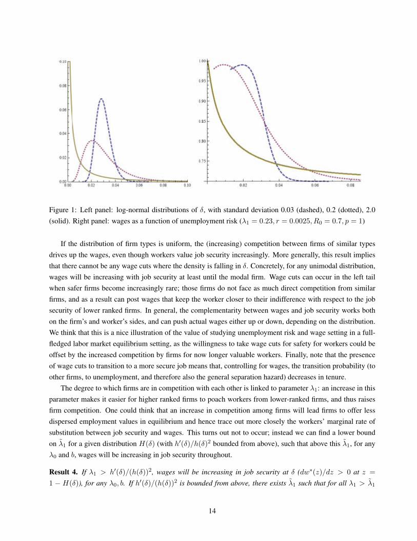
Figure 1: Left panel: log-normal distributions of δ, with standard deviation 0.03 (dashed), 0.2 (dotted), 2.0(solid). Right panel: wages as a function of unemployment risk (λ1 = 0.23, r = 0.0025, R0 = 0.7, p = 1)

If the distribution of firm types is uniform, the (increasing) competition between firms of similar typesdrives up the wages, even though workers value job security increasingly. More generally, this result impliesthat there cannot be any wage cuts where the density is falling in δ. Concretely, for any unimodal distribution,wages will be increasing with job security at least until the modal firm. Wage cuts can occur in the left tailwhen safer firms become increasingly rare; those firms do not face as much direct competition from similarfirms, and as a result can post wages that keep the worker closer to their indifference with respect to the jobsecurity of lower ranked firms. In general, the complementarity between wages and job security works bothon the firm’s and worker’s sides, and can push actual wages either up or down, depending on the distribution.We think that this is a nice illustration of the value of studying unemployment risk and wage setting in a full-fledged labor market equilibrium setting, as the willingness to take wage cuts for safety for workers could beoffset by the increased competition by firms for now longer valuable workers. Finally, note that the presenceof wage cuts to transition to a more secure job means that, controlling for wages, the transition probability (toother firms, to unemployment, and therefore also the general separation hazard) decreases in tenure.

The degree to which firms are in competition with each other is linked to parameter λ1: an increase in thisparameter makes it easier for higher ranked firms to poach workers from lower-ranked firms, and thus raisesfirm competition. One could think that an increase in competition among firms will lead firms to offer lessdispersed employment values in equilibrium and hence trace out more closely the workers’ marginal rate ofsubstitution between job security and wages. This turns out not to occur; instead we can find a lower boundon λ1 for a given distribution H(δ) (with h′(δ)/h(δ)2 bounded from above), such that above this λ1, for anyλ0 and b, wages will be increasing in job security throughout.

Result 4. If λ1 > h′(δ)/(h(δ))2, wages will be increasing in job security at δ (dw∗(z)/dz > 0 at z =

1 − H(δ)), for any λ0, b. If h′(δ)/(h(δ))2 is bounded from above, there exists λ1 such that for all λ1 > λ1

14

o ...

••

••

••

••

... .. • • • • • • • • • • • • • • • •

/t-~ ..... \ f I ".\

f I '\ ...

·,.!,.·j'~~:;.;:::::'i.¡.~;·;··:·i;.'··'· ~""":---;' ....

,.

... ••

. .. ••

········K:--', • • '. . '. . '. .

... \ '. . '. . ... \ " '\ <.

\\ \ ... . '. . '. , ",

"'L~' ..... ~ .. ~ "-" ...... . ....... ... ... ... . ..

wages are increasing in job security for all δ, for any b, λ0.

Thus, as the labor market gets more competitive, the scope for wage cuts disappears. In this result, wekeep b and λ0 constant15; while it becomes progressively easier for employed workers to move from job tojob, unemployed workers keep leaving unemployment at the same rate. This keeps the cost of losing one’sjob bounded away from zero, even as λ1 becomes very large. (In the limit: V1(δ) − V0 = p−b

r+λ+δ .) Thuswhen λ1 becomes large enough, the increased competition between firms will drive up wages with job securitythroughout the entire wage distribution, even though workers keep experiencing a loss of lifetime utility whenbecoming unemployed. Increased competition among firms does not lead to the payment of compensatingwage differentials, it does, quite surprisingly, lead to the opposite, as it strengthens the motive of the low-δfirms to compete with similar firms. To prove this, we heavily rely on the ranking property, which holds forevery λ1, and thus the firm ranking is preserved throughout any limit taking with respect to λ1 (and λ0). Thus,we can calculate firm sizes easily as a function of the rank of the firm as we approach the limit without havingto recalculate the wage distribution. In turn, firm profit maximizing decisions are then still easily characterized,following theorem 1, even as we move towards the limit, λ1 →∞.

We can also study the case where we let search frictions for both unemployed and employed workersdisappear in the limit.

Result 5. Let λ0 > λ1, λ1 →∞, λ0 →∞, while keeping λ1λ0

= α < 1 constant. Then w∗(z)→ p for all z.

If we let the frictions for the unemployed disappear, we converge to the same limit as in the standardBM model without heterogeneity in δ, which equals competitive outcome w(z) = p ∀ z, again without anycompensation for unemployment risk. To see this, note that for reservation wage out of unemployment, R0,the following holds

R0 − bp−R0

=(α− 1)

∫ 1

0

λ1(1− z)δ + λ(1− z)

δ + λ1(1− z)δ(z) + λ1(1− z)

2λ1

δ(z) + λ1(1− z)p− w∗(z)p−R0

dz (27)

≥ (α− 1)

∫ 1

0

2λ21(1− z)

(δ + λ(1− z))2dz = −2

λ1

λ1 + δ+ 2 log

δ + λ1

δ(28)

As we let λ1 go to infinity in (27), it follows that R0 → p, as the RHS goes to infinity. Since p > w∗(z) ≥ R0,it follows that all wages go to p. Since the bound in result 4 is uniform in λ0, we also know that for λ1 largeenough, wages will become increasing in job security for all δ in the process.

As we approach the competitive limit no compensating wages are paid, and all firms are still active. Inthe case where search frictions also disappear in the limit for the unemployed, job security will cease to bea payoff relevant dimension for workers. This is intuitive because, apart from the loss of ‘search capital’,there is no additional cost to unemployment.16 Decreasing λ1, λ0 means that search frictions become moreimportant, which implies that job security becomes more important, and competition between firms becomesmore limited, which raises the potential for wage cuts. Thus somewhat ironically, wage cuts, which seem torelate closely to the notion of compensating wages paid in competitive settings, are in the environment we

15Result 4 is actually stronger, it says that this bound on λ1 will hold, entirely independent of λ0 and b.16If a transition into unemployment comes with an explicit cost instead or in addition to a search cost, then in the limiting economy

only the low turnover firms would survive.

15

study actually associated with a low degree of competition among firms. Though ironic, the result is intuitive:a low λ1 means that climbing up the job ladder is a slow process in which gains are lost when becomingunemployed; therefore, at a lower λ1, workers will value job security more, ceteris paribus. Likewise, a lowerλ1 lowers the competition among firms, i.e. the relative gains of being higher in the wage ranking are lowerwhen λ1 is low, hence higher ranked firms will not increase the values (equivalent wages) that they offerworkers as much. This, however, does not mean that result 4 immediately follows from the intuition: weneed to use, explicitly, the equilibrium characterization, because the lower values offered by the firms due tothe lower competition reduce the valuation of job security, potentially more than offsetting the direct (ceterisparibus) effect of the decrease in λ1 on the workers’ valuation of job security. However, result 4 implies thatthis is not the case, and with a lower λ1 more cases can occur where firms with higher job security promise alower equivalent wage increase than is delivered by their increased job security alone, and as a result will offerlower wages, thus leading to wage cuts in equilibrium.

4 Discussion

Above we have showed that heterogeneity on the firm side alone can explain, in frictional labor markets, theabsence of compensating wages for unemployment risk and the persistence of low wages and unemploymentspells for workers. The same observations are typically explained by (additional) heterogeneity elsewhere:perhaps most prominently, persistent differences in worker qualities, or alternatively, differences in the matchqualities which need to be to some extent unknown at the start of the match. These different dimensions ofheterogeneity have further empirical implications that can be used to gauge their importance. Also, concretely,they imply differences in the risks workers face in the labor market. From this follow different implicationsfor welfare in general, and policy effectiveness in particular. While these other dimensions are doubtlesslyimportant, we argue below that a potentially large role is left open for heterogeneity in the firm-level componentof job security, and we discuss how one can distinguish the latter from other heterogeneity.

Persistent heterogeneity in worker quality In this line of explanation, we don’t see compensating wages forjob security for seemingly identical workers because the workers in low-paid, insecure jobs are in fact differentfrom those in better-paid, secure jobs. Workers’ low (unobservable) ability, however, does not in itself implythat their job durations have to be short: it is necessary to have, additionally, informational frictions or anotherdimension of heterogeneity. For example, the correlation between wages and job security could occur becauselow-ability workers are also unstable workers: they prefer not to stay with the same employer for long (Salopand Salop 1976). Alternatively, their skills are less job specific, making them more mobile (Neal 1998), orthey are repeatedly screened out during a lower-wage probationary period (Wang and Weiss 1998). Finally, toincorporate the correlation between firm characteristics with wages and job security, one can introduce firmheterogeneity such that low-ability workers sort into the relevant subset of firms. Employment in these firmsis insecure either because of aforementioned explanations, or because these firms are themselves unstable (ase.g. proposed in Evans and Leighton 1989).17

17To study this setting theoretically, one could, for example, extend the model of Albrecht and Vroman (2002) with on-the-jobsearch and increased match-breakup rates for the low productivity firms. Since this model would incorporate both firm and worker

16

If differences in persistent worker quality are indeed behind the aforementioned patterns on the labor mar-ket, every piece of a worker’s labor market history will be informative about his underlying quality, includingthe unobservable component. On the contrary, if behind these patterns is heterogeneity non-specific to theworker, in firm or match quality, the labor market history is only relevant to the extent that it is correlated withthe current firm or match quality. In this extreme case, unemployed workers –who are not in a match with afirm– are all alike, and the labor market history before the unemployment spell, or even the previous durationof the current unemployment spell, becomes irrelevant. At the same time, since being unemployed can implythat subsequent employment occurs in a lower quality match or firm, being unemployed can still predict worsefuture labor market outcomes, compared to those who remained employed. Suggestive of the importance offirm or match heterogeneity rather than worker heterogeneity is the irrelevance of previous history is the ex-perience of workers who lost their job in a mass layoff, and can expect lower wages and a higher likelihoodof repeated spells of unemployment, even when their previous labor market history was spotless (see, e.g.Stevens 1997)18 Likewise, we could test whether workers with ‘bad’ labor market histories can make theseirrelevant by finding employment in good matches or good firms. Stewart (2007) argues that this is indeed animportant feature of the labor market, while using linked employer-employee data Holzer, Lane and Vilhuber(2005) argue that good employment that allows for an escape from low earnings, is concentrated in ‘good’firms.

Thus, there are ways to econometrically identify whether diminished labor market outcomes after an un-employment spell are “due to a causal effect of being unemployed (or working) or a manifestation of a stabletrait?” (Heckman 2001). Further, it is also possible (though not necessarily easy) to distinguish the causal effectof unemployment per se, from the effect of unemployment duration, which could pick up skill depreciation ora worsening perception of unobserved quality. Controlling for observed and unobserved heterogeneity amongworkers along these lines, Arulampalam et. al. 2000 find that unemployment status per se generate a higherprobability of future unemployment spells. (They find that it explains 40% of the persistence in employmentfor mature men). Böheim and Taylor (2002) find that it is unemployment incidence, rather than duration thathas the major impact on future labor market outcomes. Recently, attention has also turned to identifying howfuture labor market outcomes are affected by being in a low-paid job – while similarly attempting to controlfor selection on unobserved quality into low-paid jobs. Although data limitations often allow only a coarsecategorization of jobs as low- or high-paid, Cappellari and Jenkins (2008), and Uhlendorf (2006) find thatbeing in a low-paid job itself increases the probability of becoming unemployed relative to the same personbeing in a high-paid job, thus showing once a worker is in unemployment, there is a risk of a low-pay/no-paycycle. All this is suggestive that there is a role to play for heterogeneity on the firm side, as argued in this

heterogeneity, it would be a good tool to measure the contribution of firm and worker heterogeneity, and their interaction. Kaas andCarrillo-Tudela (2011) show that in a setting with on-the-job search, and persistent worker heterogeneity, initially unobservable forthe firm, heterogeneity in the wage strategies can give rise to low wage employment and repeated unemployment spells of low abilityworkers.

18Plant closing arguably reduces the selection problem among workers, once it sends all workers, good or bad, to unemployment.Often it is argued that still, there is some selection issues as the workers that stay around in the firm until the final moments might notbe an unbiased sample. However, such problem can be address by including all workers who left in the years before the closure, aswell as by constructing the right control group, as e.g. in Eliason and Storrie 2006, where wage and repeat unemployment effects arestill found. See also Hijzen, Upward and Wright (2008).

17

paper.

Match Heterogeneity When match quality cannot be observed prior to forming the match, but is insteadslowly learned as time in the job increases, the unemployment hazard that results is typically initially increas-ing, then decreasing. Also, wages and job security will be positively correlated, reflecting the weeding out ofthe bad matches, and as such is consistent with the lack of compensating differentials. However, in this theory,in its most basic form, there is no role for firms. After controlling for a worker’s tenure, there should be nocorrelation of the unemployment hazard and firm characteristics. However, firm characteristics typically docorrelate significantly with the unemployment hazard after controlling for tenure (e.g. Winter-Ebmer 2001).Learning is linked to the variation of the unemployment hazard with tenure, ceteris paribus, while our paperconcerns itself with the variation in average unemployment risk across firms. It would be very interesting todecompose the variation in unemployment hazard into these across-tenure and across-firm variation.19

Looking at wages, we are further able to distinguish between ex ante known firm-specific job security andlearning. For learning theory, maintaining the standard assumption that wages are tied to expected productivity(see Moscarini 2005 for a discussion), the separation hazard goes up with tenure when one controls for wages,while in our theory it decreases with tenure. Behind this lies a different impact of uncertainty: in the case oflearning, among two matches with the same wage and thus same expected productivity, the most uncertainmatch is preferred. The reason is that the option to move out of the match insures the worker against badrealizations, diminishing the impact of the increased downside risk, while the increase in the upside riskis more fully enjoyed by the worker. In the empirically relevant setting with firm-specific job security, anincrease in uncertainty is a decrease in job security, which lowers the value of a match for a given wage.

Focussing on wage cuts, we can likewise distinguish between the two theories. In the theory of learningabout match quality, workers can move to a new match with a wage cut when the new match has a lowerexpected match quality but at the same time sufficiently more dispersion of possible outcomes, and hencemore upside potential. Then, conditional on match survival, one would observe higher wage growth after awage cut. This motive also arises elsewhere, in a different set of models where employed workers meet otherfirms occasionally, but upon such a meeting a bidding war for the worker in question is triggered (Postel-Vinayand Robin 2002, e.g.). In this setting, a worker is willing to take a lower initial wages in firms that will improvehis wage prospects for the future: either because the current firm will pay more later to retain the worker, whenit has to compete for the worker with another firm, or because the worker is able to secure a higher startingvalue when it is poached by another firm. In this case and in the case of the learning model, wage cuts are aninvestment in future wage growth. In our model, a wage cut is an investment in job security, and as such willnot show up in eventually increased wages, but in terms of increased job durations.

Connolly and Gottschalk (2008) investigate the empirical importance of this motive for wage cuts andfind that for males only 20% of the transitions with immediate wage cuts can be rationalized by future wagegrowth, thus suggesting that other factors, including job security, could be a significant driving force for wage

19It would be even better if we could use matched employer-employee data and decompose the variation into worker-specific,firm-specific and tenure-specific variation. Arai and Heyman (2001) using Swedish matched employer-employee data, is the onlypaper we know that does this; they find that tenure, worker fixed effects and firm fixed effects all turn up as significant correlates ofunemployment risk.

18

cuts. Likewise, in Postel-Vinay and Robin (2002), the option-value motive can explain a part of the extent ofdownward wage mobility, but it also leaves open a significant part for other explanations.20

Heterogeneity and risk in the labor market The amount of uncertainty a worker faces depends on therelevant dimensions of heterogeneity that underlie different outcomes. In the case of worker heterogeneity,uncertainty has resolved mostly before the labor market: workers have their own job ladders, some moreslippery than others. In the case of match heterogeneity, every transition involves a temporary increase inuncertainty when match quality in initially unknown. This means that (in the absence of firm-specific policiesthat reduce this uncertainty before the match is formed), transitions at any point in the wage ladder carry risk– though this risk might take the form of wage risk or unemployment risk, depending how good the matchlooked from an ex ante perspective (allowing for ex ante signals). Every step on the job ladder is, in somesense, taken blindly, and the worker might end up higher or lower than expected. A worker who, after learningthe match quality, stays put, is not subjecting himself to this uncertainty anymore. On the contrary, in thispaper, job transitions progressively decrease the risk of job loss, and the higher the worker is on the job ladder,the more stable he stands. A fall, however, results in a new start at the bottom of the wage ladder. Moreover,contrary to the case of learning, a there is no added uncertainty associated with taking a step, but rather a gainof stability.

All of the above three dimensions of heterogeneity imply that workers differ in their expectations of in-come and in the extent of uncertainty about this income, but each dimension has very different implicationsfor endogenous responses of workers, such as the degree of self-insurance. Workers might select a differentamount or type of human capital to avoid ending up with characteristics that lead to insecure, low-wage em-ployment. In the case of match uncertainty, risk-averse workers might save more before undertaking a riskyjob change, or stay with a current match to avoid being subject to additional uncertainty, something becomingmore important when e.g. close to a borrowing constraint.21 When jobs out of unemployment are likely atmore insecure firms, workers can improve their income security by moving to a more stable firm (as opposedto staying in a match). Foreseeing that loss of employment would raise the risk of repeat unemployment spells,employed workers might self-insure more, but as the unemployment probability at the top of the wage ladderis low while the climb back is hard, they might, ex post, still suffer a larger loss of utility upon becomingunemployed than e.g. when the unemployment risk is more evenly spread across firms.

These considerations also have implications for the public policies to allow further insurance against ad-verse income and employment shocks. If employment security is in part determined at the firm level, thenworker training might not be as effective as thought in mitigating a seeming ‘unemployment scar’, as trainedworkers might be hired by the same firms at the bottom of the firm distribution. If firm-specific unemploy-ment risk and wages are negatively correlated, workers have more dispersed lifetime discounted utilities than

20The wages generated by the simulations from the estimated model in Postel-Vinay and Robin (2002) imply a constant or lowerwage (i.e. wage cut) after the first job-to-job transition in 24%-38% of the cases, and a wage cut of five or more percent in 28.5%-42.9% of the cases. In the data on which the model is estimated, this percentage varies from 32.1%-54.5%, respectively 4.4%-22.9%for a five or more percent wage cut. These ranges are the values among the seven occupational categories on which the model isestimated separately.

21These different responses imply that one could use savings and consumption data to further distinguish between the differentdimensions of uncertainty.

19

those based on wages combined with the same, average, unemployment risk counterfactually assigned to allmatches. Then, unemployment benefits could conceivably be more beneficial than in standard settings, be-cause the expected discounted lifetime income loss upon becoming unemployed is larger when subsequentjobs are more likely to end in unemployment.22

All in all, firm-level heterogeneity in unemployment risk can provide an explanation for worker-flow andwage patterns that were the focus of this paper, but moreover, it has implications that differ from theories basedon match or worker heterogeneity. On one hand, this means that one can distinguish between these dimensionsof heterogeneity and measure their importance, and on the other hand, that care has to be taken that policiesare optimal given the measured importance of each dimension.23

Conclusion

In this paper, we have presented a model with homogeneous workers and search frictions in which, in equi-librium, wages do not compensate for differences in unemployment risk. Therefore, workers move, wheneverthey have the chance, from risky companies to more stable firms, which then are also larger. We show thatwages increase with job security for the lowest wages; this pattern can extend over a significant part of thewage distribution. While safer firms can offer lower wages while still attracting more workers, the increasedjob duration makes a worker more valuable to the firm, and hence raises their incentive to prevent workermobility to other firms, which puts an upwards force on wages. The second force dominates at low wages, buthigher in the wage distribution, depending on the distribution of the heterogeneous firms, the first force candominate – thus leading to wage cuts.

The model also generates an unemployment hazard rate that is declining with tenure, as in the data, whilein the standard Burdett and Mortensen (1998) model it is counterfactually constant. We thus show that unem-ployment scarring in terms of wages and risk of repeated job losses, arises in equilibrium, resulting neitherfrom an decline in (perceived) productivity of workers when they become unemployed, nor as a manifestationof a selection effect on workers, but because of heterogeneity on the firm side.

References

[1] Abowd, J. M. and O. Ashenfelter (1981): "Anticipated Unemployment, Temporary Layoffs, and Com-pensating Wage Differentials", in: Rosen, S., ed., Studies in Labor Markets , University of ChicagoPress;

[2] Abowd, J. M., R. H. Creecy and F. Kramarz (2002): "Computing Person and Firm Effects Using LinkedLongitudinal Employer-Employee Data", mimeo;

22Moreover, the moral hazard implications of unemployment benefits might be different when separations into unemployment aredriven in part by firm characteristics (and firms’ choices), rather than workers’ choices, though this also necessitates an appropriatecontracting friction that drives a wedge between the two.

23Another example where allowing firm-heterogeneity, in addition to match heterogeneity, can lead to different conclusions, is Kahn(2008). She finds that those hired in recessions have lower job durations, but that this is driven by the selection of firms that hire inrecessions, rather than an on average worse quality of the matches formed in a recession.

20

[3] Akerlof, G. and B. Main (1980): "Unemployment Spells and Unemployment Experience", AmericanEconomic Review, 70(5), 885-893;

[4] Albrecht, J. and S. Vroman (2002): "A Matching Model with Endogenous Skill Requirements", Interna-tional Economic Review, 43(1), 283-305;

[5] Arai, M. and F. Heyman (2001): "Wages, Profit and Individual Employment Risk: Evidence frommatched worker-firm data.", FIEF working paper;

[6] Arulampalam, W., Booth, A.L., and Taylor, M.P. (2000): "Unemployment persistence", Oxford EconomicPapers, 52(1), 24-50;

[7] Boheim, R. and M. P. Taylor (2002): "The search for success: do the unemployed find stable employ-ment?", Labour Economics, 9, 717-735;

[8] Brugemann, B. (2008): "Empirical Implications of Joint Wealth Maximizing Turnover", mimeo;

[9] Burdett, K. and D.T. Mortensen (1980): "Search, Layoffs, and Market Equilibrium" Journal of PoliticalEconomy, 88, 652-672;

[10] Burdett,K. and D.T. Mortensen (1998): "Wage Differentials, Employer Size and Unemployment", Inter-national Economic Review, 39, 257-273;

[11] Carneiro, A. and P. Portugal, "Wages and the Risk of Displacement", in Polachek, S. and K. Tatsiramos(ed.): Work, Earnings and Other Aspects of the Employment Relation (Research in Labor Economics,Volume 28), pp.251-276

[12] Coles, M. (2001): "Equilibrium Wage Dispersion, Firm Size, and Growth", Review of Economic Dynam-ics,4 (1), 159-187;

[13] Davis, S., Haltiwanger, J. and S. Schuh (1996): Job Creation and Job Destruction, MIT Press;

[14] Eliason, M. and D. Storrie (2006): "Lasting or Latent Scars? Swedish Evidence on the Long-TermEffects of Job Displacement", Journal of Labor Economics, 24(4), 831-856;

[15] Evans, D. and L. S. Leighton (1989): "Why Do Smaller Firms Pay Less", Journal of Human Resources,24(2), 299-318;

[16] Farber, H. and R. Gibbons (1996): "Learning and Wage Dynamics", Quarterly Journal of Economics,111(4), 1007-1047;

[17] Hwang, H., D. Mortensen and W. Reed (1998): "Hedonic Wages and Labor Market Search", Journal ofLabor Economics, 16 (4), 815-847;

[18] Heckman, J.J. (2001): "Micro data, heterogeneity, and the evaluation of public policy: Nobel lecture",Journal of Political Economy, 109(4), 673–748;

21

[19] Idson, T. L. and W. Y. Oi (1999): ”Firm Size and Wages” in Ashenfelter, O. and D.Card (eds.): Handbookof Labor Economics, Volume 3(B), 2165-2214;

[20] Jovanovic, B. (1979): "Job Matching and the Theory of Turnover", Journal of Political Economy, 87(5),972-990;

[21] Jovanovic, B. (1982): "Selection and the evolution of Industry", Econometrica, 50(3), 649-670;

[22] Jovanovic, B. (1984): "Matching, Turnover, and Unemployment", Journal of Political Economy, 92(1),108-122;

[23] Mayo, J. W. and M. N. Murray (1991): "Firm size, employment risk and wages: further insights on apersistent puzzle", Applied Economics, 23, 1351-1360;

[24] Moretti, E. (2000): "Do Wages Compensate for Risk of Unemployment? Parametric and SemiparametricEvidence from Seasonal Jobs", Journal of Risk and Uncertainty, 20 (1), 45-66;

[25] Mortensen, D.T. (1990): "Equilibrium Wage Distributions: A Synthesis" in Hartog,J., G. Ridder, and J.Theeuwes (eds.), Panel Data and Labor Market Studies, Amsterdam: North Holland;

[26] Moscarini, G. (2005 ): "Job Matching and the Wage Distribution", Econometrica, 73(2), 481-516

[27] Moscarini, G. and F. Postel-Vinay (2010 ): "Stochastic Search Equilibrium", Cowles Foundation Discus-sion Paper 1754, Oct. 2010

[28] Neal, D. (1998): "The Link between Ability and Specialization: An Explanation for Observed Correla-tions between Wages and Mobility Rates ", Journal of Human Resources, 33(1), 173-200;

[29] Pinheiro, R. and L. Visschers (2006): "Job Security and Wage Differentials", mimeo;

[30] Postel-Vinay, F. and J.-M. Robin (2002a): “The Distribution of Earnings in an Equilibrium Search Modelwith State-Dependent Offers and Counter-Offers”, International Economic Review, 43 (4), 989-1016;

[31] Postel-Vinay, F. and J.-M. Robin (2002b): “Wage Dispersion with Worker and Employer Heterogeneity”,Econometrica, 70(6), 2295-2350;

[32] Rubinstein, Y. and Y. Weiss (2006): "Post Schooling Wage Growth: Investment, Search and Learning"in Hanushek, E. and F. Welch (eds.): Handbook of the Economics of Education, Vol. 1, 1-67;

[33] Ruhm, C. (1991): "Are Workers Permanently Scarred by Job Displacements?", American EconomicReview, 81(1), 319-324;

[34] Salop, J. and S. Salop (1976): "Self-Selection and Turnover in the Labor Market", The Quarterly Journalof Economics, 90(4), 619-627;

[35] Salvanes, K. G. (2005): "Employment policies at the plant level: Job and Worker Flows for heteroge-neous Labour in Norway", mimeo;

22

[36] Stevens, A.H. (1997): "The importance of multiple job losses", Journal of Labor Economics, 15(1),165-188;

[37] Stewart, M.B. (2007): "The inter-related dynamics of unemployment and low pay", Journal of AppliedEconometrics, 22(3), 511–531

[38] Topel, R. (1993): "What have we learned from Empirical Studies of Unemployment and Turnover?",American Economic Review P&P, 83(2), 110-115;

[39] Wang, R. and A. Weiss (1998): "Probation, layoffs, and wage-tenure profiles: A sorting explanation",Labour Economics, 5(3), 359-383;

[40] Winter-Ebmer, R. (2001): "Firm Size, Earnings and Displacement Risk", Economic Inquiry, 39, 474-486;

[41] Winter-Ebmer, R. and J. Zweimuller (1999): "Firm Size Wage Differentials in Switzerland: Evidencefrom Job Changers", American Economic Review P&P, 89, 89-93.

APPENDIX

A Proofs

Proof of lemma 1 The initial conditions (6) follow directly from putting V (w, δ) − V0 = 0 in (3). For (4),note first that it can be established straightforwardly that V (w, δ) is continuous, increasing and bounded in w,and therefore differentiable a.e., and therefore it follows that the same properties also hold for w∗(ws, δ) by(3). The value of employment at (w, δ) satisfies

(r + δ)V (ws, δ) = ws + δV0 + λ1

∫ ∫w∗(ws,δ)

V (w′, δ′s, δ)dF (w′|δ′)dH(δ′). (29)

=⇒ ∂V (ws, δ)

∂ws=

1

r + δ + λ1

∫ ∫ ww∗(ws,δ) dF (w′|δ′)dH(δ′)

, a.e. (30)

where we have used that the derivative with respect to lower bound of the inner integral, w∗(ws, δ), equalszero for every δ, since it is evaluated where V (w∗(ws, δ), δ) = V (ws, δ). Using (3) and (29), the latter both

23

evaluated at V (w, δ) and V0 = V (R0, δ), we have

w∗(ws, δ) = ws + (δ − δ)

((r + δ)−1

(ws −R0 − λ1

(∫ ∫ w∗(ws,δ′)

R0

V (w′, δ′)dF (w′|δ′)dH(δ′)

+

∫ ∫ w

w∗(ws,δ′)V (ws, δ)dF (w′|δ′)dH(δ′)−

∫ ∫ w

R0

V0dF (w′|δ′)dH(δ′)

))(31)

=⇒ ∂w∗(ws, δ)

∂ws=r + δ

r + δ− (δ − δ)

r + δλ1

∫ ∫w∗(ws,δ′)

dF (w′|δ′)dH(δ′)∂V (ws, δ)

∂ws

=r + δ + λ1

∫ ∫w∗(ws,δ′) dF (w′|δ′)dH(δ′)

r + δ + λ1

∫ ∫w∗(ws,δ′) dF (w′|δ′)dH(δ′)

, a.e. (32)

and (4) now follows. For (5) note that ∂w∗(ws,δ)∂δ = V (ws, δ) − V0 = w∗(ws,δ)−ws

δ−δ . The second derivativesfollow from straightforward differentiation.

Proof of lemma 2 In this proof, we show that the appropriate ratio of limits of a sequence of sets agreeswith (9) almost everywhere (with respect to F (w, δ)). (We do not have to worry about a set of measure zerofor overall outcomes: anything that happens on a set of measure zero won’t affect the profit maximization ofother agents, or is otherwise relevant for outcomes in equilibrium. Hence, if we can establish l(ws, δ) a.e. weare done.) First, we can define

I(δ, ws)def=

∫δ′≤δ,R0≤ws′≤ws

(δ′ + λ1

∫ws>ws

dF (ws, δ) + λ1

∫δ>δ,

ws≥ws>ws′dF (ws, δ)

)dG(ws′, δ′)(m− u)

−∫δ′≤δ,R0≤ws′≤ws

(λ0u+ λ1

∫δ>δ,ws<ws′

dG(ws, δ)(m− u)

)dF (ws′, δ′)

(33)

Then, for δ′′ > δ′ and ws′′ > ws′, we have I(δ′′, ws′′)− I(δ′, ws′′)− I(δ′′, ws′) + I(δ′, ws′) = 0. After sometedious algebra, in which we drop the terms (i.e. flows) that cancel each other out, add up the remaining flowswhere possible, but split the integral such that in one set the upper bound is not included and in the other setthe wage to integrate over is a singleton {ws′′}; this results in∫

δ′<δ≤δ′′ws′<w<ws′′

(δ + λ1

∫ws>ws′′

dF (ws, δ) + λ1

∫δ /∈(δ′,δ′′]w<w≤ws′′

dF (w, δ)

)dG(w, δ)

+

∫δ′<δ≤δ′′w=ws′′

(δ + λ1

∫ws>ws′′

dF (ws, δ)

)dG(w, δ)

=

∫δ′<δ≤δ′′

ws′<w<ws′′

(λ0u+ λ1

∫ws≤ws′

dG(ws, δ) + λ1

∫δ /∈(δ′,δ′′]ws′≤w<w

dG(w, δ)

)dF (w, δ)

+

∫δ′<δ≤δ′′w=ws′′

(λ0u+ λ1

∫ws≤ws′

dG(ws, δ)

)dF (w, δ) (34)

Now, we can take the limit as δ′ → δ′′ and ws′ → ws′′. There are two cases: (i)∫w=ws′′,all δ dF (w, δ) = 0,

and (ii)∫w=ws′′,all δ dF (w, δ) > 0. In case (i), the terms on the second and fourth line equal zero, while

24

the rightmost terms in the integral on the first and third line are equal in value to an integral that has a strictupper or lower on wages, i.e. λ1

∫δ /∈(δ′,δ′′]w<w≤ws′′

dF (w, δ) = λ1

∫δ /∈(δ′,δ′′]w<w<ws′′

dF (w, δ)def= T (w, δ′). Moreover, T is

continuous at (δ′′, ws′′) with T (δ′′, ws′′) = 0 , so we have

(δ+λ1(1−F (ws′′))

lim δ′→δ′′ws′→ws′′

∫δ′<δ<δ′′

ws′<w≤ws′′dG(w, δ)

lim δ′→δ′′ws′→ws′′

∫δ′<δ<δ′′

ws′<w≤ws′′dF (w, δ)

= (δ+λ1(1−F (ws′′))l(ws′′, δ) = λ0u+λG(ws′′),

using that dG(ws′′,δ)dF (ws′′,δ) = l(ws′′, δ), and that G(ws′′), F (ws′′) are continuous at ws′′. Rearranging yields (9).

For case (ii), we can first take the limit ws′ → ws′′ on both sides of the equation. The terms on the first andthird line go to zero. If the second and fourth line are zero as well, we are dealing a set {(ws, δ)|ws = ws′′, δ ∈(δ′, δ′′]} that is of measure zero in F , which wlog for the aggregate patterns, we can ignore. Suppose thereforethat B(δ′, δ′′)

def= {(ws, δ)|ws = ws′′, δ ∈ (δ′, δ′′]} is of positive measure. Then in the limit as ws′ → ws′′

(34) reduces to∫δ′<δ≤δ′′w=ws′′

(δ + λ1

∫ws>ws′′

dF (ws, δ)

)dG(w, δ) =

∫δ′<δ≤δ′′w=ws′′

(λ0u+ λ1

∫ws<ws′′

dG(ws, δ)

)dF (w, δ)

(35)

Consider now the limit as δ′ → δ′′ while B(δ′, δ′′) stays of positive measure (if it becomes of zero measure,we can ignore it, wlog). The terms between brackets inside the integrals stay constant, and hence can be takenoutside the integrals. Dividing both sides by

∫δ′<δ≤δ′′w=ws′′

dF (w, δ), and taking the limit wrt δ, we have

(δ+λ1(1−F+(ws′′))

limδ′→δ′′∫δ′<δ≤δ′′ws′=ws′′

dG(w, δ)

limδ′→δ′′∫δ′<δ≤δ′′ws′=ws′′

dF (w, δ)= (δ+λ1(1−F+(ws′′))l(ws′′, δ) = λ0u+λG−(ws′′),

where (1− F+(ws′′) =∫ws>ws′′ dF (ws, δ) and G−(ws) =

∫ws<ws′′ dG(ws, δ). �

Proof of proposition 1 Suppose there exists equivalent wages wB, wA, such that wB > wA, and wB isoffered by the more risky firm while wA by the more solid firm. Then it must be that

(p− w∗(wB, δh))l(wB, δh) ≥ (p− w∗(wA, δl))l(wA, δh). (36)

Now, note the following, by (9) l(ws,δl)l(ws,δh) = δh+λ1(1−F (ws))

δl+λ1(1−F (ws)) > 1 and both right and left derivatives of this

ratio with respect to ws are λ1F ′i (ws)(δh−δl)

(δl+λ1(1−F (ws)))2 ≥ 0 with i = {L,R}. Therefore, this ratio is larger than 1 andincreasing, and in particular

l(wB, δl)

l(wA, δl)≥ l(wB, δh)

l(wA, δh). (37)

To study the instantaneous profit per worker, notice

d(p−w∗(ws,δl)p−w∗(ws,δh)

)dws

=−dw∗(ws,δl)

dws (p− w∗ (ws, δh)) + dw∗(ws,δh)dws (p− w∗(ws, δl))

(p− w∗ (w, δh))2 > 0

25

since p− w∗(ws, δl) > p− w∗(ws, δl) for ws > R0, and dw∗(ws,δ)dws is strictly increasing in δ for all ws, all by

lemma 1. But this impliesp− w∗(wB, δl)p− w∗(wA, δl)

>p− w∗(wB, δh)

p− w∗(wA, δh). (38)

Now, putting (37) and (38) together, it follows that (36) implies

(p− w∗(wB, δl))l(wB, δl) > (p− w∗(wA, δl))l(wA, δl),

which contradicts that wA was the profit maximizing choice of the solid firm. �

Proof of proposition 2. First, the same argument that established thatG(ws, δ) is absolutely continuous withrespect to F (ws, δ) can be made to establish that F (ws, δ) is absolutely continuous with respect to G(ws, δ),which then necessarily implies that each property (i)-(iii) applies to F (ws), if and only if it applies to G(w).

To establish property (ii), towards a contradiction, consider a ws at which a strictly positive mass of wagesis offered, with δ1 as the infimum of those types offering this equivalent wage. The expected profit gain forthis type when offering a wage ws + ε is greater than

dπ

dε= −

(dw∗(ws, δ)

dwsε+ ξ(ε)

)l(ws, δ1) + (p− w∗(ws, δ))λ1G

−(ws + ε)− λ1G−(ws)

λ1(1− F+(ws)) + δ1, (39)

where ξ(ε) is a term with ξ(ε)ε → 0 as ε → 0. Note that a mass point at ws implies that, there exists a η > 0,

such that for all ε > 0, G−(ws + ε) − G−(ws) ≥ 2η(λ1+1)λ1

> 0. Then, as ε → 0, dπdε > η. Moreover, sincedw∗(ws,δ)

dws is continuous by (4), this also holds for a δ2 > δ1 close enough to δ1, in particular δ2 is also closeenough to δ1 to offer equivalent wage ws to workers. This δ2 then has a profitable deviation, which is thecontradiction we were looking for. This establishes the absence of mass points, and hence the continuity ofF (ws) and G(ws).

Next, consider the case where the support of F (ws) is not connected. Let ws be the minimum equivalentwage in the support of F (ws), and ws the corresponding maximum wage. Then, there exist ws < ws1 < ws2 <

ws such that F (ws1) = F (ws2), and G(ws1) = G(ws2) by the continuity of F (ws), G(ws). Consider a firmposting at ws2, this firm can keep the same firm size but make strictly more profit when deviating to ws. Ifws > R0, the same argument applies: the firm offering ws can deviate to R0, which does not affect his firmsize, but strictly raises the profit per worker. �

Proof of theorem 1 There are three steps in this proof. First, one can show that the equilibrium objectsF (ws), G(ws), w∗(w, δ), F (w|δ), R0 constructed fromw∗(z), ws(z) satisfy workers’ and firms’ optimization.This is straightforward, with this and the derivation in the paper, we have established that a steady stateequilibrium corresponds to {ws(z), w∗(z), R0} and vice versa.24

Pseudoconcavity of the firm’s problem Secondly, we have to check that the first-order conditions indeedpick the maximum in the firm’s problem, at any point where δ(z) is continuous. We can verify that the problem

24For completeness, this in appendix B.

26

is pseudo-concave, using (4) and (17) by showing the expression below is negative when (18) holds.

d

dz′

((p− w∗(ws(z′), δ(z)))∂l

d(z′, δ(z))

∂z′−(∂w∗(ws(z′), δ(z))

∂ws(z′)

dws(z′)

dz′

)ld(z′, δ(z))

)(40)

Evaluated at a point where the first order condition is equal to zero (z = z′), this has the same sign as

∂

∂z′

((p− w∗(ws(z′), δ(z))) 2λ1

λ1(1− z′) + δ(z)

)− ∂

∂z′

(∂w∗(ws(z′), δ(z))

∂ws(z′)

∂ws(z′)

∂z′

)(41)

At a z = z′ the first term equals− 4λ21

(λ1(1−z)+δ(z))2 (p−w∗(ws(z), δ(z)))+2λ2

1(λ1(1−z)+δ(z))2 (p−w∗(ws(z), δ(z)))

which reduces to− 2λ21

(λ1(1−z)+δ(z))2 (p−w∗(ws(z), δ(z))). The second term equals ∂2w∗(ws,δ)∂ws∂ws

(dws

dz

)2+∂w∗

∂wsd2ws

dzdz .Focussing on the last term, differentiating (21) wrt z, we find that it equals

−dw∗(z)

dz

2λ1

λ1(1− z) + δ+ (p− w∗(z)) 2λ2

1

(λ1(1− z) + δ)2+

(p− w∗) 2λ1

λ1(1− z) + δ

λ1(δ − δ)(r + δ + λ(1− z))2

dw∗(ws, δ)

dws(42)

By (22), dw∗(z)dz < (p − w∗(z)) 2λ2

1(λ1(1−z)+δ) , and therefore in absolute value the first two terms of the expres-

sion above jointly are smaller than (p − w∗(z)) 2λ21

(λ1(1−z)+δ)2 . The last term in (42) is negative, and is equal

−∂2w∗(ws,δ)∂ws∂ws

(dws

dz

)2. Substituting the above in (40), and canceling out terms yields that d

dz′

(·)< 0.

Existence and uniqueness of the fixed point R0. Finally, we have to show existence and uniqueness of thereservation wage R0 = ws(0) = w∗(0) satisfying (21), (22), (24). From this, the existence and uniqueness ofthe steady state equilibrium then follows. Index dws(z;R0)

dz , dw∗(z;R0)dz by their initial conditions R0; then (24)

is the solution to the following fixed point

R0 = T (R0), where T (R0) = b+ (λ0 − λ1)

∫ 1

0

1− zr + λ1(1− z) + δ

dws(z;R0)

dzdz (43)

Note that dws(z)dz depends implicitly on the reservation only through (p− w∗(z)).

Manipulating (21) and (22), we can find

d(p− w∗(z))dz

= −(p− w∗(z))(

2λ1

λ1(1− z) + δ(z)+

δ′(z)

δ(z)− δx(z)

)(44)

dx(z)

dz=

2λ1

λ1(1− z) + δ(z)

δ(z)− δr + λ1(1− z) + δ(z)

+

(δ′(z)

δ(z)− δ+

2λ1

δ(z) + λ1(1− z)

)x(z) +

δ′(z)

δ(z)− δx(z)2,

(45)

where x(z) = w∗(z)−ws(z)p−w∗(z) . Note that p − w∗(0) = p − R0, and x(0) = 0. Note that d(p−w∗(z))

dR0, by standard

FODE theory, is continuous in R0. Consider first the interval [0, z] on which δ(z) is continuous. On thisinterval, x(z) does not depend on R0. We can rewrite (44) to get

d(p−w∗(z))dz

(p− w∗(z))= −

(2λ1

δ(z) + λ1(1− z)+ δ′(z)x(z)

); (46)

27

Integrating over z yields

p− w∗(z) = e−∫ z0

(2λ1

δ(z)+λ1(1−z) +δ′(z)x(z))dz

(p−R0), (47)

where the exponential term does not depend on R0. It follows immediately that

d(p− w∗(z))dR0

= −e−∫ z0

(2λ1

δ(z)+λ1(1−z) +δ′(z)x(z))dz< 0.

To generalize this to general distributionsH(δ), consider next a point where δ(z) is discontinuous: this a pointwhere δ(z) drops discretely. We want to show that the properties of d(p−w∗(z))

dR0, dx(z)dR0

are preserved. Considerfirst x(z), from (23),

(p− w∗(z))x(z) =δ(z)− δ

limz↑z δ(z)− δ

(limz↑z

(p− w∗(z))x(z)

). (48)

Alternatively, the limit limz↑z y(z) = yL(z) for any variable y, and δ(z)−δδL(z)−δ = ∆ we can rewrite (23) as

w∗ = ∆(w∗L(z)− ws(z))− ws(z) (49)

=⇒ (p− w∗(z)) = (p− w∗L(z))(1 + (1−∆)xL(z)). (50)

From the previous results then, given d(p−w∗L(z))dR < 0, dxL(z)

dR = 0 combined with (50), it follows thatd(p−w∗(z))

dR < 0; and thus, d(p−w∗(z))dR is preserved when δ(z) drops discretely.

Equation (50) tells us that d ln(p−w∗(z))dR =

d ln(p−w∗L(z))dR + d ln(1+(1−∆)xL(z))

dR . Rewriting (48) similarly,using (50), we find

x(z) =∆xL(z)

1 + (1−∆)xL(z), (51)

from which it follows that dx(z)dR = 0 whenever dxL(z)

dR = 0. Thus, the irresponsiveness of dx(z)dR is also

preserved whenever δ(z) drops discretely. Let Z = {ζi} be the countable set of ranks at which δ(z) dropsdiscretely; define additionally ζ0 = 0. Then, letting ζ(z) = sup{ζ ∈ Z|ζ < z}

p− w∗(z) = (p−R0)

∏{i|ζi∈Z,ζi<z}

e−∫ ζiζi−1

(2λ1

δ(z′)+λ1(1−z′) +δ′(z′)x(z′))dz′

(1 + (1−∆(ζi))xL(ζi))

·e−∫ zζ(z)

(2λ1

δ(z′)+λ1(1−z′) +δ′(z′)x(z′))

(52)

From this it follows that d(p−w∗(z))dR0

= −S(z) < 0, where S(z) is the entire term postmultiplying (p−R0) onthe RHS of (52). It is negative and does not vary with R0. 25

25A similar result holds true in the standard Burdett and Mortensen model, where

p− w(z) = (p−R0)

(λ1(1− z) + δ

λ1 + δ

)2

,

however, here we have take care of the heterogeneity in δ, and the resulting influence on the wages (with wage cuts etc.). Notice thatif we set δ′(z) = 0 and hence ∆(z) = 0 and x(z) = 0 ∀z, the Burdett and Mortensen result in fact follows. We find it encouragingthat a similar nice property can be derived in our more complicated setting.

28

To consider existence, note that T (p) = b, and for λ0 ≥ λ1 ≥ 0 T (b) ≥ b, while T (R0) is continuous inR0, as dws(z;R0)

dz is continuous inR0, since, from the above, (p−w∗(z)) is continuous inR0. For 0 < λ0 < λ1,because T (R0) = b + (λ0 − λ1)

∫(V (w; δ) − V0)dF (w; δ) and

∫(V (w; δ) − V0)dF (w; δ) is bounded by

p−br , and hence T (R0) is bounded from below by b − λ1

p−br , as we let R0 go negatively enough, eventually

T (R0) > R0.To consider uniqueness, notice that the slope of T (R0) does not depends on R0. Hence, there can only be

at most one intersection with R0. (Since T (p) = b < p, we can rule out the case that T (R0) has slope 1, andhas a continuum of equilibrium). �.

Proof of Result 1 The inflow into employment λ0u+ λG(z) = l(z)(δ(z) + λ(1− z)), the probability thatan inflow at time t survives until t + τ is e(δ(z)+λ1(1−z))τ ; thus the number of workers in the zth firm whohave been around τ periods teu(z, τ)

def= l(z)(δ(z) + λ(1 − z)e−(δ(z)+λ(1−z))τ . Then, the derivative of the

empirical hazard rate with respect to tenure is

d ln

(∫ 10 δ(z)teu(z, τ)dz∫ 1

0 teu(z, τ)dz

)/dτ = −

∫ 1

0

(δ(z)− δave)teu(z, τ) (δ(z) + λ1(1− z))dz∫δaveteu(z′, τ)dz′

< 0 (53)

The derivative dteu(z, τ)/dτ = −teu(z, τ)(δ(z)+λ1(1−z)). Define δave∫teu(z′, τ)dz′ =

∫δ(z′)teu(z′, τ)dz′.

Then∫ 1

0 (δ(z)− δave)teu(z, τ)dz equals zero; since δ(z)− δave and (δ + λ1(1− z)) are both decreasing, thelatter one strictly, the integral term in (53) is positive, establishing the result.

Proof of Result 2 By proposition 1, locally, for z close 0, we have w∗(z) strictly increasing. Then thereexists z > 0 such that w∗(z) is strictly increasing for all 0 < z < z, and by (21) so is ws(z). Now, supposethat there exists a sequence {zn} with zn < z, such that w∗(zn)→ R0. By (3), then also ws(zn)→ R0. Then,there exists an n, such that ws(zn) < ws(z), contradicting the ranking property.

Proof of Result 3 Note that since dw∗(0)/dz > 0, at the the z from which onwards an interval of wage cutsoccurs, both dw∗(z)/dz = 0 and d2w∗(z)/(dzdz) < 0, i.e. dw∗(z)/dz cuts 0 from above, at z . The secondderivative at z equals

d2w∗

dzdz= −dw

∗

dz

2λ1

λ1(1− z) + δ(z)+ (p− w∗(z)) 2λ1(λ1 − δ′(z))

(λ1(1− z) + δ(z))2+ δ′′(V (ws(z), δ)− V0)

+ δ′(z)1

r + δ + λ1(1− z)dws

dz. (54)

Note that after substituting in dws(z)/dz from (21), the terms with δ′(z) cancel out. Evaluated at a pointwhere dw∗/dz = 0, and letting r → 0, this turns into

d2w∗

dzdz

∣∣∣∣dw∗dz

=0

= (p− w∗(z)) 2λ21

(λ1(1− z) + δ(z))2+ δ′′(V (ws(z), δ)− V0) (55)

This can be smaller than zero only if δ′′(z) < 0, which in turn occurs if and only if h′(δ) > 0, since δ′(z) =

−1/h(δ) and δ′′(z) = h′(δ)h(δ)2 δ

′(z).

29

The second point follows from (22) being negative. Substituting in ws(z) into (22), a change of theintegrating variable (dz = −h(δ)dδ), this can be written equivalently as

(p− w∗(1−H(δ)))2λ1

δ + λ1(1−H(δ))<

1

h′(δ)

∫ δ

δ

2λ1(δ + λ1(1−H(δ)))

(δ + λ(1−H(δ)))3(p− w∗(1−H(δ)))h(δ)dδ

Since p− w∗(δ(1−H(δ))) > p− w∗(δ) for δ > δ, the above equation is negative whenever (26) holds.

Proof of Result 4 We can show this by establishing that d2w∗(z)dwdw < 0, and dw∗(z)

dz = 0 cannot occur forλ1 >

h′(δ)(h(δ))2 .Note that the existence of wage cuts implies a z such that dw∗(z)/dz = 0, d

2w∗(z)dzdz ≤ 0. This

implies that at that z, from (22) and (55),

(p− w∗(z)) 2(λn1 )2

δ(z) + λ1(1− z)< −δ′′(z)

∫ z

0

1

δ(z′) + λ1(1− z′)dws(z′)

dz′dz (56)

(p− w∗(z)) 2λ1

δ(z) + λ1(1− z)= −δ′(z)

∫ z

0

1

δ(z′) + λ1(1− z′)dws(z′)

dz′dz (57)

Dividing the RHS of (56) by the RHS of (56), and similarly for the LHS, this yields

λ1 < δ′′(z)/δ′(z) =h′(δ)

(h(δ))2

as a necessary condition. Hence if λ1 >h′(δ)

(h(δ))2 , we do not satisfy the necessary condition, and therefore canrule out dw∗(z)/dz < 0 at z = 1−H(δ).

Proof of Result 5 is in the main text

30

B Additional Material

proof of proposition 1, verification In the paper, we derived {ws(z), w∗(z), R0} satisfying (21), (22), (24)from the equilibrium conditions. Here, we outline the reverse argument: any set {ws(z), w∗(z), R0} satis-fying (21), (22) and (24) corresponds to a steady state equilibrium. Since we have established that the tuple{ws(z), w∗(z), R0} satisfying the aforementioned conditions exists and is unique, we have also establishedexistence and uniqueness of the steady state equilibrium.

The rest of proof consists of the rather straightforward construction of equilibrium. We construct (i) the ag-gregate conditions, (ii) the worker’s optimization, (iii) firm’s optimization. First invert ω = ws(z), to constructF (ω) = (ws)−1(ω), G(ws) = Gz(ws)−1(ω) at ws = ws(z), and w∗(ws, δ) for those wages that are actuallyposted on the equilibrium path from w∗(ws, δ) = {w∗(z)|ws = ws(z), δ = δ(z) for some z}. Then wecan construct F (w|δ) from F (ws), δ(z), w∗(ws, δ). F (ws, δ), G(ws, δ) can be constructed straightforwardlyfrom F (ws), δ(z). Now we have to show that these distribution are consistent with optimal decision making,(ii)-(iii). Given F (ws), w∗(ws, δ), where for off-equilibrium (ws, δ) we use the same partial derivatives as inlemma 1, to derive the entire function w∗(ws, δ). For worker optimization and firm optimization, consider thatfirms choose ws in the profit maximization, which leads to the following first order condition

(p− w∗(ws(z), δ(z)))∂l(ws, δ)

∂ws−(∂w∗(ws, δ)

∂ws

)l(ws, δ) = 0, (58)

which can be rewritten as

∂w∗(ws,δ)∂ws

p− w∗(ws(z), δ(z))−

∂l(ws,δ)∂ws

l(ws, δ)= 0, ⇐⇒

∂w∗(ws,δ)∂ws

p− w∗(ws(z), δ(z))=

2λ1F′(ws)

δ + λ(1− F (ws))(59)

Using F ′(ws) = 1/ws′(z), we can verify that (17) and (19) combined with (21) and (22) imply (4)-(5)and the equivalence of (58) and (17), thus establishing both w∗(ws, δ) = w∗(ws, δ) and the optimality ofz = F−1(ws). Finally, the equivalence of R0 can be established by a simple change of variable in the integral(24).

31