Tracing Ray Differentials

Homan Igehy

Computer Science Department

Stanford University

AbstractAntialiasing of ray traced images is typically performed by super-sampling the image plane. While this type of filtering works wellfor many algorithms, it is much more efficient to perform filteringlocally on a surface for algorithms such as texture mapping. Inorder to perform this type of filtering, one must not only trace theray passing through the pixel, but also have some approximationof the distance to neighboring rays hitting the surface (i.e., a ray’sfootprint). In this paper, we present a fast, simple, robust schemefor tracking such a quantity based on ray differentials, derivativesof the ray with respect to the image plane.

CR Categories and Subject Descriptors: I.3.7 [ComputerGraphics]: Three-Dimensional Graphics and Realism – color,shading, shadowing, and texture; raytracing.

1 INTRODUCTIONRay tracing [18] is an image generation technique that is able toaccurately model many phenomena which are difficult orimpossible to produce with a traditional graphics pipeline. Aswith any image synthesis algorithm, ray tracing is prone toaliasing, and antialiasing is typically performed by tracing rays atmultiple sub-pixel offsets on the image plane (e.g., [12, 18]). Bystochastically point sampling each of many variables per ray [6],one may filter over multiple phenomena simultaneously. Forsome algorithms, however, it is much more efficient to filter overa more local domain. For example, in texture mapping, a texturewill often be viewed under high minification so that the entiretexture falls under a small number of pixels. Filtering such atexture by taking bilinear samples for a set of stochastic raysrequires the tracing of a correspondingly large number of rays.This is problematic because the cost of tracing a ray is relativelyhigh, and the minification factor can be arbitrarily high. On theother hand, if we knew the distance between a ray and the rays fora neighboring pixel when the ray hit the texture map (i.e., a ray’sfootprint), then we could efficiently filter the texture by using afast, memory coherent algorithm such as mip mapping [19].Tracing such a quantity in a polygon rendering pipeline isstraightforward because primitives are drawn in raster order, and

the transformation between texture space and image space isdescribed by a linear projective map [10]. In a ray tracer,however, the primitives are accessed according to a pixel’s raytree, and the transformation between texture space and imagespace is non-linear (reflection and refraction can make raysconverge, diverge, or both), making the problem substantiallymore difficult.

Tracing a ray’s footprint is also important for algorithms otherthan texture mapping. A few of these algorithms are listed below:

§ Geometric level-of-detail allows a system to simultaneouslyantialias the geometric detail of an object, bound the cost oftracing a ray against an object, and provide memory coherentaccess to the data of an object. However, to pick a level-of-detail, one must know an approximation of the ray densitywhen a ray is intersected against an object.

§ When ray tracing caustics, the intensity attributed to asampled light ray depends upon the convergence ordivergence of the wavefront [13]. Similarly, in illuminationmapping, the flux carried by a ray from a light source mustbe deposited over an area on a surface’s illumination mapbased on the density of rays [5].

§ Dull reflections may be modeled by filtering textures over akernel which extends beyond the ray’s actual footprint [2].

In this paper, we introduce a novel approach for quickly androbustly tracking an approximation to a ray’s footprint based onray differentials. Ray tracing can be viewed as the evaluation ofthe position and direction of a ray as the ray propagates throughthe scene. Because a ray is initially parameterized in terms ofimage space coordinates, in addition to tracing the ray, we canalso trace the value of its derivatives with respect to the imageplane. A first-order Taylor approximation based on thesederivatives gives an estimate of a ray’s footprint. A fewtechniques for estimating ray density have been presented in theliterature [2, 5, 13, 16], but ray differentials are faster, simpler,and more robust than these algorithms. In particular, because raydifferentials are based on elementary differential calculus ratherthan on differential geometry or another mathematical foundationthat has an understanding of the 3D world, the technique may bereadily applied to non-physical phenomena such as bumpmapping and normal-interpolated triangles. General formulae fortracing ray differentials are derived for transfer, reflection, andrefraction, and specific formulae are derived for handling normal-interpolated triangles. Finally, we demonstrate the utility of raydifferentials in performing texture filtering.

2 RELATED WORKSeveral algorithms have been developed for estimating a texturefiltering kernel in polygon rendering pipelines (e.g., [1, 10]).Similar algorithms have been used in ray tracers that calculate theprojection of texture coordinates onto the image plane [8], but

homan@graphics.stanford.edu

such a projection is only valid for eye rays. This technique can beextended to reflected and refracted rays by computing the totaldistance traveled, but such an approximation is invalid becausecurved surfaces can greatly modify the convergence or divergenceof rays. A few algorithms have been developed that take this intoaccount, and we will review them briefly.

Within the context of a ray tracer, finite differencing has beenused to calculate the extent over which a light ray’s illuminance isdeposited on an illumination map by examining the illuminationmap coordinates of neighboring rays [5]. The main advantage offinite differencing is that it can easily handle any kind of surface.The main disadvantages, however, are the difficult problemsassociated with robustly handling neighboring eye rays whose raytrees differ. The algorithm must detect when a neighboring raydoes not hit the same primitives and handle this case specially.One plausible method of handling such a case is to send out aspecial neighboring ray that follows the same ray tree andintersects the plane of the same triangles beyond the triangleedges, but this will not work for spheres and other higher-orderprimitives. Additionally, this special case becomes the commoncase as neighboring rays intersect different primitives that arereally part of the same object (e.g., a triangle mesh). Ouralgorithm circumvents these difficulties by utilizing thedifferential quantities of a single ray independently of itsneighbors.

Cone tracing [2] is a method in which a conical approximationto a ray’s footprint is traced for each ray. This cone is used foredge antialiasing in addition to texture filtering. The mainproblem with a conical approximation is that a cone is isotropic.Not only does this mean that pixels must be sampled isotropicallyon the image plane, but when the ray footprint becomesanisotropic after reflection or refraction, it must be re-approximated with an isotropic footprint. Thus, this methodcannot be used for algorithms such as anisotropic texture filtering.In addition, extending the technique to support surfaces other thanplanar polygons and spheres in not straightforward.

Wavefront tracing [9] is a method in which the properties of adifferentially small area of a ray’s wavefront surface is tracked,and it has been used to calculate caustic intensities resulting fromillumination off of curved surfaces [13]. Wavefronts have alsobeen used to calculate the focusing characteristics of the humaneye [11]. Although highly interrelated, the main differencebetween wavefronts and our method of ray differentials is that ourmethod tracks the directional properties of a differentially smalldistance while wavefront tracing tracks the surface properties of adifferentially small area. Thus, wavefronts cannot handleanisotropic spacing between pixel samples. Additionally, becausea differential area is an inherently more complex quantity, thecomputational steps associated with wavefront tracing are morecomplicated. Wavefront tracing is based on differential geometrywhile our algorithm is based on elementary differential calculus,and a technical consequence of this is that we can readily handlenon-physically based phenomena such as normal-interpolatedtriangles, bump mapped surfaces, and other algorithms that areself-contradicting in the framework of differential geometry. Apractical consequence of being based on the simpler field ofelementary differential calculus is that our formulation is easier tounderstand, and extending the technique to handle differentphenomena is straightforward.

Paraxial ray theory [4] is an approximation techniqueoriginally developed for lens design, and its application to raytracing is known as pencil tracing [16]. In pencil tracing, paraxialrays to an axial ray are parameterized by point-vector pairs on a

plane perpendicular to the axial ray. The propagation of theseparaxial rays is approximated linearly by a system matrix. Aswith wavefront tracing, the computational complexity of penciltracing is significantly higher than our method. Additionally,pencil tracing makes a distinct set of simplifying assumptions tomake each phenomenon linear with respect to the system matrix.An approximation is made even on transfer, a phenomenon that islinear with respect to a ray. Furthermore, the handling of non-physical phenomena is unclear. By comparison, the single unifiedapproximation we make is simply that of a first-order Taylorapproximation to a ray function.

3 TRACING RAY DIFFERENTIALSOne way to view ray tracing is as the evaluation of the positionand direction of a ray function at discrete points as it propagatesthrough the scene. Any value v that is computed for the ray (e.g.,luminance, texture coordinate on a surface, etc.) is derived byapplying a series of functions to some initial set of parameters,typically the image space coordinates x and y:

( )( )( )( )yxv nn ,ffff 121 K−= (1)

We can compute the derivative of this value with respect to animage space coordinate (e.g., x) by applying the Chain Rule:

xxv

n

n

∂∂

∂∂

∂∂

∂∂

−= 1

1

2

1

fff

ff

K (2)

As transformations are applied to a ray to model propagationthrough a scene, we are just applying a set of functions fi to keeptrack of the ray. We can also keep track of ray differentials,derivatives of the ray with respect to image space coordinates, byapplying the derivatives of the functions. These ray differentialscan then be used to give a first-order Taylor approximation to theray as a function of image space coordinates. In the forthcomingderivations, we express scalars in italics and points, directions,and planes with homogeneous coordinates in bold.

A ray can be parameterized by a point representing a positionon the ray and unit vector representing its direction:

DPR =v

(3)

The initial values for a ray depend on the parameterization of theimage plane: a pinhole camera is described by an eye point, aviewing direction, a right direction, and an up direction. Thedirection of a ray going through a pixel on the image plane can beexpressed as a linear combination of these directions:

( ) UpRightViewd yxyx ++=, (4)

Thus, the eye ray is given by:

( )( )

( ) 21,

,

dddD

EyeP

⋅=

=

yx

yx(5)

We can now ask the question, given a ray, if we were to pick aray slightly above or to the right of it on the image plane, what raywould result? Each of these differentially offset rays can berepresented by a pair of directions we call ray differentials:

yyy

xxx

∂∂

∂∂

∂∂

∂∂

∂∂

∂∂

=

=

DPR

DPR

v

v

(6)

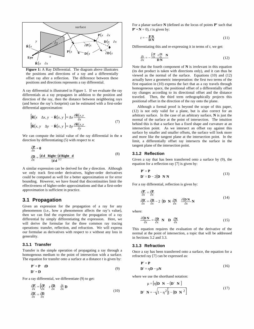
A ray differential is illustrated in Figure 1. If we evaluate the raydifferentials as a ray propagates in addition to the position anddirection of the ray, then the distance between neighboring rays(and hence the ray’s footprint) can be estimated with a first-orderdifferential approximation:

( ) ( )[ ] ( )

( ) ( )[ ] ( )y

yx

xyx

yyxyyx

xyxyxx

∂∂

∂∂

∆≈−∆+

∆≈−∆+

,

,

,,

,,

R

R

RR

RRv

v

vv

vv

(7)

We can compute the initial value of the ray differential in the xdirection by differentiating (5) with respect to x:

( ) ( )( ) 23dd

dRightdRightddD

P 0

⋅⋅−⋅

∂∂

∂∂

=

=

x

x(8)

A similar expression can be derived for the y direction. Althoughwe only track first-order derivatives, higher-order derivativescould be computed as well for a better approximation or for errorbounding. However, we have found that discontinuities limit theeffectiveness of higher-order approximations and that a first-orderapproximation is sufficient in practice.

3.1 PropagationGiven an expression for the propagation of a ray for anyphenomenon (i.e., how a phenomenon affects the ray’s value),then we can find the expression for the propagation of a raydifferential by simply differentiating the expression. Here, wewill derive the formulae for the three common ray tracingoperations: transfer, reflection, and refraction. We will expressour formulae as derivatives with respect to x without any loss ingenerality.

3.1.1 TransferTransfer is the simple operation of propagating a ray through ahomogenous medium to the point of intersection with a surface.The equation for transfer onto a surface at a distance t is given by:

DD

DPP

=′+=′ t

(9)

For a ray differential, we differentiate (9) to get:

( )xx

xt

xxxt

∂∂

∂′∂

∂∂

∂∂

∂∂

∂′∂

=

++=

DD

DPP D(10)

For a planar surface N (defined as the locus of points P′′ such thatP′′ • N = 0), t is given by:

NDNP⋅⋅−=t (11)

Differentiating this and re-expressing it in terms of t, we get:

( )ND

NDP

⋅⋅+

∂∂ ∂

∂∂∂

−= xxt

xt (12)

Note that the fourth component of N is irrelevant in this equation(its dot product is taken with directions only), and it can thus beviewed as the normal of the surface. Equations (10) and (12)actually have a geometric interpretation: the first two terms of thefirst equation in (10) express the fact that as a ray travels throughhomogeneous space, the positional offset of a differentially offsetray changes according to its directional offset and the distancetraveled. Then, the third term orthographically projects thispositional offset in the direction of the ray onto the plane.

Although a formal proof is beyond the scope of this paper,(12) is not only valid for a plane, but is also correct for anarbitrary surface. In the case of an arbitrary surface, N is just thenormal of the surface at the point of intersection. The intuitionbehind this is that a surface has a fixed shape and curvature at anintersection point. As we intersect an offset ray against thissurface by smaller and smaller offsets, the surface will look moreand more like the tangent plane at the intersection point. In thelimit, a differentially offset ray intersects the surface in thetangent plane of the intersection point.

3.1.2 ReflectionGiven a ray that has been transferred onto a surface by (9), theequation for a reflection ray [7] is given by:

( )NNDDD

PP

⋅−=′=′

2(13)

For a ray differential, reflection is given by:

( ) ( )

+⋅−=

=

∂⋅∂

∂∂

∂∂

∂′∂

∂∂

∂′∂

NND NDNDD

PP

xxxx

xx

2(14)

where:

( )xxx ∂

∂∂∂

∂⋅∂ ⋅+⋅= NDND DN (15)

This equation requires the evaluation of the derivative of thenormal at the point of intersection, a topic that will be addressedin Sections 3.2 and 3.3.

3.1.3 RefractionOnce a ray has been transferred onto a surface, the equation for arefracted ray [7] can be expressed as:

NDD

PP

µ−η=′=′

(16)

where we use the shorthand notation:

( ) ( )[ ]

( )[ ]22 11 NDND

NDND

⋅−η−−=⋅′

⋅′−⋅η=µ(17)

x

y

( )xP

( )xP∂

( )xD∂Eye

surface

x∂

( )xx ∂+Rv

( )xRv

( )xx ∂+D

( )xx ∂+P

( )xD

Figure 1: A Ray Differential. The diagram above illustratesthe positions and directions of a ray and a differentiallyoffset ray after a reflection. The difference between thesepositions and directions represents a ray differential.

and η is the ratio of the incident index of refraction to thetransmitted index of refraction. Differentiating, we get:

+µ−η=

=

∂µ∂

∂∂

∂∂

∂′∂

∂∂

∂′∂

NNDD

PP

xxxx

xx(18)

where (referring to (15) from Section 3.1.2):

( )( )

( )xx ∂⋅∂

⋅′⋅η

∂µ∂

−η= ND

NDND2

(19)

3.2 Surface NormalsThe formulae derived for reflection and refraction of raydifferentials in Sections 3.1.2 and 3.1.3 depend on the derivativeof the unit normal with respect to x. In differential geometry [17],the shape operator (S) is defined as the negative derivative of aunit normal with respect to a direction tangent to the surface. Thisoperator completely describes a differentially small area on asurface. For our computation, the tangent direction of interest isgiven by the derivative of the ray’s intersection point, and thus:

( )xx ∂

∂∂∂ −= PN S (20)

For a planar surface, the shape operator is just zero. For a sphere,the shape operator given a unit tangent vector is the tangent vectorscaled by the inverse of the sphere’s radius. Formulae for theshape operator of both parametric and implicit surfaces may befound in texts on differential geometry (e.g., [17]) and othersources [13], and thus will not be covered here in further detail.

3.3 DiscussionOne interesting consequence of casting ray differentials in theframework of elementary differential calculus is that we mayforgo any understanding of surfaces and differential geometry,even in expressing the derivative of a unit normal. For thatmatter, we may forgo the geometric interpretation of anycalculation, such as the interpretation made for equations (10) and(12). For example, if we know that the equation of a unit normalto a sphere with origin O and radius r at a point P on the sphere isgiven by:

( ) rOPN −= (21)

then we may “blindly” differentiate with respect to x to get:

rxx ∂

∂∂∂ = PN (22)

This differentiation may be performed on any surface or for anyphenomenon. If we know the formula for how a ray is affected bya phenomenon, then we can differentiate it to get a formula forhow a ray differential is affected without any understanding of thephenomenon. For example, if we apply an affine transformationto a ray so that we may perform intersections in object spacecoordinates, then the ray differential is transformed according tothe derivative of the affine transformation. If we apply an ad hocnon-linear warp to rays in order to simulate a fish-eye lens effect,then we can derive an expression for warping the ray differentialsby differentiating the warping function. This is a large advantageof being based on elementary differential calculus rather than on aphysically-based mathematical framework.

In graphics, we often use non-physical surfaces that separatethe geometric normal from the shading normal, such as normal-interpolated triangles or bump mapped surfaces. For suchsurfaces, the use of ray differentials is straightforward. In the caseof transfer to the point of intersection, the geometric normal isused for (12) because a neighboring ray would intersect thesurface according to the shape defined by the geometric normal.For reflection and refraction, however, the shading normal is usedbecause neighboring rays would be reflected and refractedaccording to the shading normal. Because of its common use, wederive an expression for the derivative of the shading normal for anormal-interpolated triangle in the box below.

The computational cost of tracing ray differentials is verysmall relative to the other costs of a ray tracer. Each of the

Normal-Interpolated TrianglesThe position of a point P on the plane of a triangle may beexpressed as a linear combination of the vertices of triangle:

γβα γ+β+α= PPPP

where the barycentric weights α, β, and γ are all positive when Pis inside the triangle and add up to one when P is on the plane ofthe triangle. These values may be calculated as the dot productbetween the point P expressed in normalized homogeneouscoordinates (i.e., w=1) and a set of planes Lα, Lβ, and Lγ:

( )( )( ) PLP

PLP

PLP

⋅=γ

⋅=β

⋅=α

γ

β

α

Lα can be any plane that contains Pβ and Pγ (e.g., one that isperpendicular to the triangle), and its coefficients are normalizedso that Lα• Pα = 1; Lβ and Lγ can be computed similarly. Thenormal at a point is then computed as a linear combination of thenormals at the vertices:

( ) ( ) ( )

( ) 21nnnN

NPLNPLNPLn

⋅

γγββαα

=

⋅+⋅+⋅=

Differentiating, we get:

( ) ( ) ( )( ) ( )

( ) 23nn

nnnnN

PPPn

nn

NLNLNL

⋅

⋅−⋅∂∂

γ∂∂

γβ∂∂

βα∂∂

α∂∂

∂∂

∂∂

=

⋅+⋅+⋅=

xxx

xxxx

where a direction (e.g., the derivative of P) is expressed inhomogeneous coordinates (i.e., w=0). The sum of the threebarycentric weights for the derivative of P add up to zero whenthe direction is in the plane of the triangle.

Similarly, a texture coordinate can be expressed as a linearcombination of the texture coordinates at the vertices:

( ) ( ) ( ) γγββαα ⋅+⋅+⋅= TPLTPLTPLT

and its derivative is given by:

( ) ( ) ( ) γ∂∂

γβ∂∂

βα∂∂

α∂∂ ⋅+⋅+⋅= TLTLTL PPPT

xxxx

interactions in Section 3.1 requires a few dozen floating-pointoperations. On a very rough scale, this is approximately the samecost as a single ray-triangle intersection, a simple lightingcalculation, or a step through a hierarchical acceleration structure,thus making the incremental cost insignificant in all but thesimplest of scenes.

4 TEXTURE FILTERINGOne practical application of ray differentials is texture filtering. Ifwe can approximate the difference between the texturecoordinates corresponding to a ray and its neighboring rays, thenwe can find the size and shape of a filtering kernel in texturespace. The texture coordinates of a surface depend on the textureparameterization of the surface. Such a parameterization isstraightforward for parametric surfaces, and algorithms exist toparameterize implicit surfaces [14]. In general, the texturecoordinates of a surface may be expressed as a function of theintersection point:

( )PT f= (23)

We can differentiate with respect to x to get a function that isdependent on the intersection point and its derivative:

( )[ ] ( )xxx ∂

∂∂

∂∂∂ == PPT P,gf (24)

We also derive the expression for the derivative of texturecoordinates for a triangle in the box on the previous page.

Applying a first-order Taylor approximation, we get anexpression for the extent of a pixel’s footprint in texture spacebased on the pixel-to-pixel spacing:

( ) ( )[ ]( ) ( )[ ]

yy

xx

yyxyyx

xyxyxx

∂∂∂∂

∆≈−∆+=∆

∆≈−∆+=∆

T

T

TTT

TTT

,,

,,(25)

4.1 Filtering AlgorithmsAssuming texture coordinates are two-dimensional, (25) defines aparallelogram over which we filter the texture. This is illustratedby Figure 2. Given this parallelogram, one of several texturefiltering methods can be used. The most common method, mipmapping [19], is based on storing a pyramid of pre-filteredimages, each at power of two resolutions. Then, when a filteredsample is required during rendering, a bilinearly interpolatedsample is taken from the level of the image pyramid that mostclosely matches the filtering footprint. There are many ways ofselecting this level-of-detail, and a popular algorithm [10] is basedon the texel-to-pixel ratio defined by the length of the larger axisof the parallelogram of Figure 2:

( ) ( )

∆⋅∆∆⋅∆=

2121,maxlog2 yyxxlod TTTT (26)

Because the computed level-of-detail can fall in between imagepyramid levels, one must round this value to pick a single level.In order to make the transition between pyramid levels smooth,systems will often interpolate between the two adjacent levels,resulting in trilinearly interpolated mip mapping.

Mip mapping is an isotropic texture filtering technique thatdoes not take into account the orientation of a pixel’s footprint.When using (26), textures are blurred excessively in one direction

if the parallelogram defined by (25) is asymmetric. Anisotropicfiltering techniques take into account both the orientation and theamount of anisotropy in the footprint. A typical method [3, 15] isto define a rotated rectangle based on the longer of the two axes ofthe parallelogram, use the rectangle’s minor axis to choose a mipmap level, and average bilinear samples taken along the majoraxis. Again, one may interpolate between mip map levels.

4.2 ResultsFigure 3 and Figure 4 demonstrate a scene rendered with four

approaches towards texture filtering, all generated with a singleeye ray per pixel at a resolution of 1000 by 666. In this scene,which consists entirely of texture mapped triangles, we are at adesk that is in a room with a wallpaper texture map for its wallsand a picture of a zebra in the woods on the left. We are viewinga soccer ball paper weight on top of a sheet of text, and we areexamining the text with a magnifying glass.

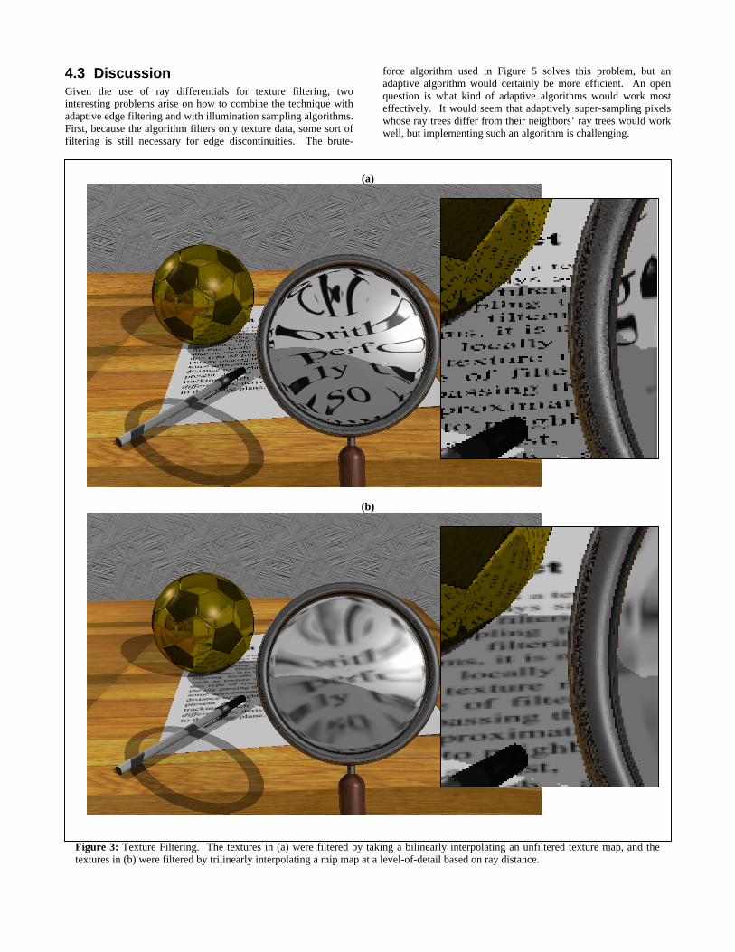
In Figure 3a, we perform texture filtering by doing a simplebilinear filtering on the texture map. The text in this image isnoticeably aliased in the three places where minification isoccurring: on the paper, in the reflection off of the ball, andaround the edges of the lens. Additionally, the reflection of thewalls and the zebra in the soccer ball is very noisy. This aliasingis also apparent on the frame of the magnifying glass, especiallyon the left edge as the zebra is minified down to only a few pixelson the x direction. Even at sixteen rays per pixel (not shown), thisartifact is visible.

In Figure 3b, mip mapping is performed for texture lookups,and the level-of-detail value is calculated based on the distance aray has traveled and projection onto the surface. The textures ofthe image are properly filtered for eye rays, but reflected andrefracted rays use the wrong level-of-detail. For the reflections,the divergence of the rays increases because of the surfacecurvature, and thus the level-of-detail based on ray distance is toolow. This results in aliasing off of the ball and the frame. Forrefraction, the rays converge, making the ray distance-basedalgorithm cause blurring.

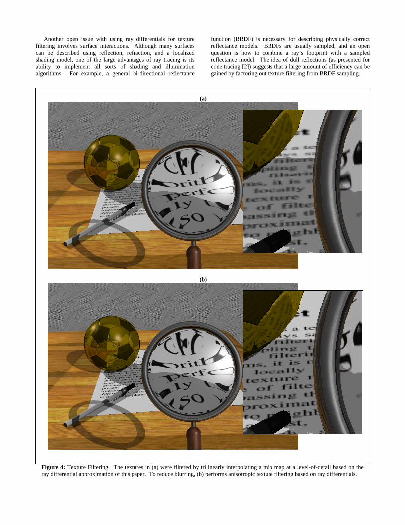
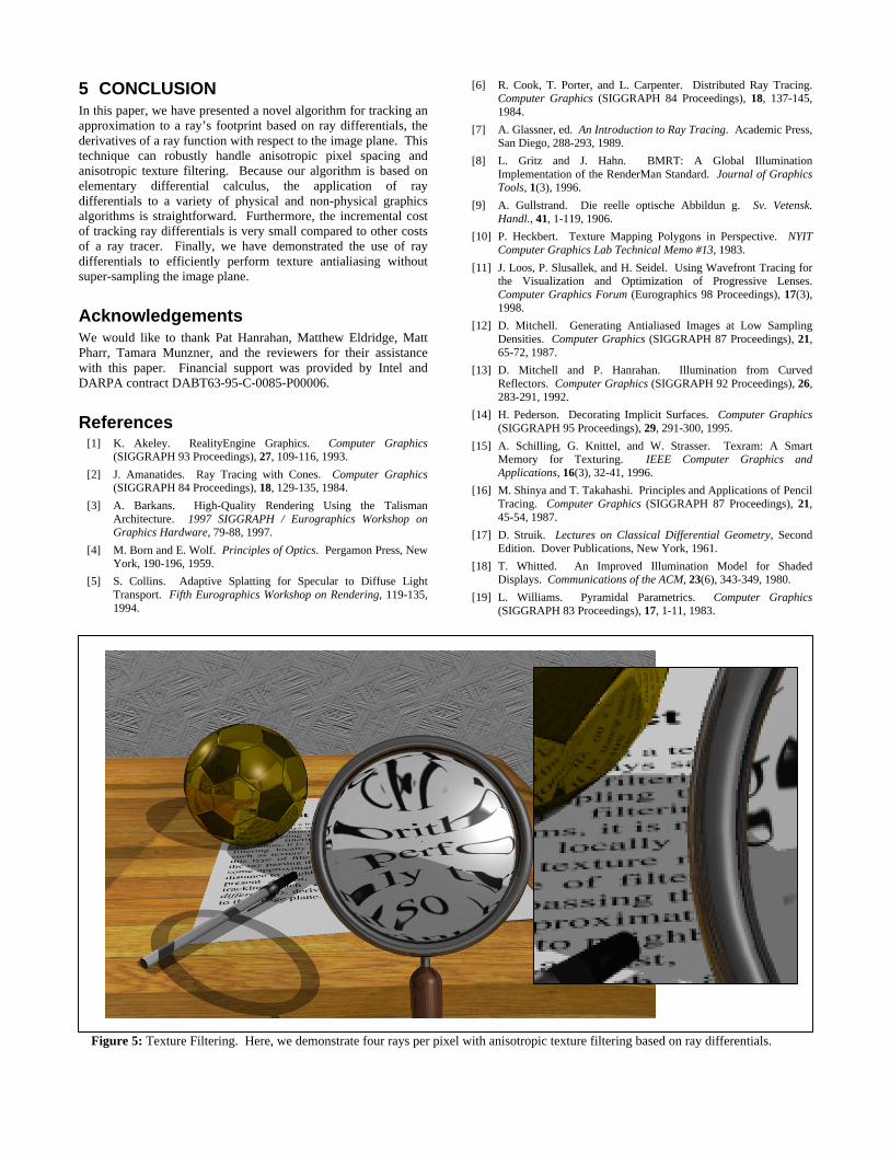
In Figure 4a, we perform mip mapping with the level-of-detailbeing computed by ray differentials. The limitations of thisisotropic filtering are most apparent in the text. In order toaddress the blurring of the text on the paper, in the reflection offthe ball, and around the edges of the lens, we demonstrateanisotropic texture filtering in Figure 4b. This image still hasvisible aliasing due to silhouette edges and shadowingdiscontinuities, and Figure 5 demonstrates that a simple super-sampling of 4 rays per pixel combined with anisotropic texturefiltering produces a relatively alias-free image.

x u

vy

Image Space Texture Space

xT∆

yT∆

Figure 2: Texture Filtering Kernel. A pixel’s footprint inimage space can map to an arbitrary region in texture space.This region can be estimated by a parallelogram formed by afirst-order differential approximation of the ratios betweenrate of change in texture space and image space coordinates.

4.3 DiscussionGiven the use of ray differentials for texture filtering, twointeresting problems arise on how to combine the technique withadaptive edge filtering and with illumination sampling algorithms.First, because the algorithm filters only texture data, some sort offiltering is still necessary for edge discontinuities. The brute-

force algorithm used in Figure 5 solves this problem, but anadaptive algorithm would certainly be more efficient. An openquestion is what kind of adaptive algorithms would work mosteffectively. It would seem that adaptively super-sampling pixelswhose ray trees differ from their neighbors’ ray trees would workwell, but implementing such an algorithm is challenging.

(a)

(b)

Figure 3: Texture Filtering. The textures in (a) were filtered by taking a bilinearly interpolating an unfiltered texture map, and thetextures in (b) were filtered by trilinearly interpolating a mip map at a level-of-detail based on ray distance.

Another open issue with using ray differentials for texturefiltering involves surface interactions. Although many surfacescan be described using reflection, refraction, and a localizedshading model, one of the large advantages of ray tracing is itsability to implement all sorts of shading and illuminationalgorithms. For example, a general bi-directional reflectance

function (BRDF) is necessary for describing physically correctreflectance models. BRDFs are usually sampled, and an openquestion is how to combine a ray’s footprint with a sampledreflectance model. The idea of dull reflections (as presented forcone tracing [2]) suggests that a large amount of efficiency can begained by factoring out texture filtering from BRDF sampling.

(a)

(b)

Figure 4: Texture Filtering. The textures in (a) were filtered by trilinearly interpolating a mip map at a level-of-detail based on theray differential approximation of this paper. To reduce blurring, (b) performs anisotropic texture filtering based on ray differentials.

5 CONCLUSIONIn this paper, we have presented a novel algorithm for tracking anapproximation to a ray’s footprint based on ray differentials, thederivatives of a ray function with respect to the image plane. Thistechnique can robustly handle anisotropic pixel spacing andanisotropic texture filtering. Because our algorithm is based onelementary differential calculus, the application of raydifferentials to a variety of physical and non-physical graphicsalgorithms is straightforward. Furthermore, the incremental costof tracking ray differentials is very small compared to other costsof a ray tracer. Finally, we have demonstrated the use of raydifferentials to efficiently perform texture antialiasing withoutsuper-sampling the image plane.

AcknowledgementsWe would like to thank Pat Hanrahan, Matthew Eldridge, MattPharr, Tamara Munzner, and the reviewers for their assistancewith this paper. Financial support was provided by Intel andDARPA contract DABT63-95-C-0085-P00006.

References[1] K. Akeley. RealityEngine Graphics. Computer Graphics

(SIGGRAPH 93 Proceedings), 27, 109-116, 1993.

[2] J. Amanatides. Ray Tracing with Cones. Computer Graphics(SIGGRAPH 84 Proceedings), 18, 129-135, 1984.

[3] A. Barkans. High-Quality Rendering Using the TalismanArchitecture. 1997 SIGGRAPH / Eurographics Workshop onGraphics Hardware, 79-88, 1997.

[4] M. Born and E. Wolf. Principles of Optics. Pergamon Press, NewYork, 190-196, 1959.

[5] S. Collins. Adaptive Splatting for Specular to Diffuse LightTransport. Fifth Eurographics Workshop on Rendering, 119-135,1994.

[6] R. Cook, T. Porter, and L. Carpenter. Distributed Ray Tracing.Computer Graphics (SIGGRAPH 84 Proceedings), 18, 137-145,1984.

[7] A. Glassner, ed. An Introduction to Ray Tracing. Academic Press,San Diego, 288-293, 1989.

[8] L. Gritz and J. Hahn. BMRT: A Global IlluminationImplementation of the RenderMan Standard. Journal of GraphicsTools, 1(3), 1996.

[9] A. Gullstrand. Die reelle optische Abbildun g. Sv. Vetensk.Handl., 41, 1-119, 1906.

[10] P. Heckbert. Texture Mapping Polygons in Perspective. NYITComputer Graphics Lab Technical Memo #13, 1983.

[11] J. Loos, P. Slusallek, and H. Seidel. Using Wavefront Tracing forthe Visualization and Optimization of Progressive Lenses.Computer Graphics Forum (Eurographics 98 Proceedings), 17(3),1998.

[12] D. Mitchell. Generating Antialiased Images at Low SamplingDensities. Computer Graphics (SIGGRAPH 87 Proceedings), 21,65-72, 1987.

[13] D. Mitchell and P. Hanrahan. Illumination from CurvedReflectors. Computer Graphics (SIGGRAPH 92 Proceedings), 26,283-291, 1992.

[14] H. Pederson. Decorating Implicit Surfaces. Computer Graphics(SIGGRAPH 95 Proceedings), 29, 291-300, 1995.

[15] A. Schilling, G. Knittel, and W. Strasser. Texram: A SmartMemory for Texturing. IEEE Computer Graphics andApplications, 16(3), 32-41, 1996.

[16] M. Shinya and T. Takahashi. Principles and Applications of PencilTracing. Computer Graphics (SIGGRAPH 87 Proceedings), 21,45-54, 1987.

[17] D. Struik. Lectures on Classical Differential Geometry, SecondEdition. Dover Publications, New York, 1961.

[18] T. Whitted. An Improved Illumination Model for ShadedDisplays. Communications of the ACM, 23(6), 343-349, 1980.

[19] L. Williams. Pyramidal Parametrics. Computer Graphics(SIGGRAPH 83 Proceedings), 17, 1-11, 1983.

Figure 5: Texture Filtering. Here, we demonstrate four rays per pixel with anisotropic texture filtering based on ray differentials.