A 3-D RAY TRACING MODEL FOR MACROCELL URBAN ENVIRONMENTS AND ITS VERIFICATION WITH

MEASUREMENTS T. Fügen*, S. Knörzer*, M. Landmann†, R.S. Thomä†, W. Wiesbeck*

*Institut für Höchstfrequenztechnik und Elektronik, Universität Karlsruhe (TH), Germany, †Technische Universität Ilmenau, Fachgebiet Elektronische Messtechnik, Germany

e-mail: Thomas.Fuegen@ihe.uka.de

Keywords: 3-D ray tracing, MIMO measurements, RIMAX, delay spread, azimuth spread.

Abstract

This paper presents verification results of an advanced 3-D ray tracing model in a macrocell urban environment. The verification is based on wide-band double-directional channel measurements at a center frequency of 5.2 GHz and a bandwidth of 120 MHz. For the verification two site-specific measurement routes in the city center of Karlsruhe, Germany are used. Both, the wide-band and the directional prediction of the ray tracing are evaluated. For the verification of the directional prediction the maximum-likelihood channel parameter estimation framework RIMAX is applied to the measurement data. Results show a strong level of agreement of delay spread and azimuth spread.

1 Introduction

The successful design of MIMO systems requires a detailed understanding and knowledge of the radio propagation channel. For that reason, it is important first to set up a double directional MIMO channel model and second to verify the model in order to ensure that it describes the spatio-temporal propagation channel and the wide variety of channel-induced effects in MIMO systems in an accurate way. Various MIMO channel models have been reported in the literature in recent years [1 - 5]. Depending on the modeling philosophy, they can be categorized in stochastic and deterministic. Many papers address the adjustment and validation of stochastic MIMO channel models. But only few references are available that deal with the verification of the joint temporal and spatial as well as of the MIMO properties of deterministic models [6]. The aim of this paper is to partly close this gap. Deterministic models are based on a detailed simulation of the actual physical wave propagation process in a deterministically described scenario. The modeling of the propagation phenomena is usually based on geometrical optics (GO) and the uniform geometrical theory of diffraction (UTD). As the determination of the multipaths between a specific transmitter (Tx) and receiver (Rx) point is based on ray concepts, it is referred as ray tracing [7]. Traditional ray

tracing models take reflection and diffraction into account. However, it has been shown by measurements, that the proportion of power coming from nonspecular contributions, so called dense or diffuse multipaths, can be significantly high [8]. Since diffuse scattering increases the multipath richness it has a noticeable impact on the temporal and angular dispersion and the MIMO performance [9]. As a consequence diffuse scattering models have been developed and implemented into the ray concept [10, 11]. The 3-D ray tracing model used in this study contains models for diffuse scattering on trees and buildings. A detailed verification of the non-directional narrow- and wide-band properties of the propagation channel with measurements at 2 GHz was given in [12]. Additionally, verification results of the one-directional channel at the base station site at 5.2 GHz were presented. All verified properties are showing a good agreement with measurements. This paper will present a supplemented verification of the double-directional properties of the 3-D ray tracing model at 5.2 GHz. The paper is organized as follows: Section 2 gives a brief review of the 3-D ray tracing model. Next, an overview of the MIMO measurement setup and the measurement environment is given. To allow for comparison between the angular behavior of the ray tracing model and the MIMO measurements, the gradient-based maximum-likelihood channel parameter estimation framework RIMAX is applied to the measurement data [13]. A brief summary of the RIMAX algorithm is given in Section 4. Section 4 also presents the verification results.

2 Description of the 3-D Ray Tracing Model The 3-D ray tracing model consists of two major parts: a realistic model of the propagation environment and a model to calculate the multi-path wave propagation between the transmitter and the receiver [12]. As environment data a digital model of a part of the city of Karlsruhe, Germany, is used (cf. Fig. 1). It includes buildings, trees and the street floor. Buildings are generated by means of a vector data set that describes their exact position and size. Each building is modeled as a box with a certain rooftop type (e.g. flat roof, pitched roof, hipped roof). It is assumed that on average all buildings have constitutive parameters of dry

concrete (εr = 5 - j0.1, µr = 1). For proper wave propagation modeling it is essential to include huge trees into the model. Only the tree crown is taken into account, the tree trunk is neglected. The crown is modeled as a box, with an average height of 3 m above ground. The exact position and size of the trees is determined from a morphographic data set. For the street floor concrete with a surface roughness of σ = 1 mm is used (εr = 5 - j0.1, µr = 1) [13].

Fig. 1: Model of the measurement scenario with transmitter Tx1 and receiver Rx1 and Rx2 A ray-optical wave propagation tool is used to calculate the channel between the transmitter and the receiver. It distinguishes between different multi-path components. Each path is represented by a ray, which may consecutively experience several different propagation phenomena. The propagation phenomena taken into account in the channel model are combinations of multiple reflections and multiple diffractions as well as single scattering. The modified Fresnel reflection coefficients, which account for slightly rough surfaces, are used to model the reflections [15]. In order to trace pure reflection paths, the method of image transmitters (image theory) is implemented [18]. Diffraction is described by the UTD and the corresponding heuristic coefficients for lossy wedge diffraction [16]. Moreover, the UTD slope diffraction coefficients according to [16] are used to enhance the accuracy, especially for multiple diffractions. Since the proposed propagation model supports full 3-D~diffraction, Fermat's principle is used to determine the diffracted ray paths [15]. For mixed paths image theory and Fermat's principle are combined. Real objects such as buildings or trees have no perfectly flat surface. Buildings for example, exhibit a variety of irregularities, e.g. windows, balconies, eaves gutters, etc. If the wave-length is in the order of the dimensions of these irregularities, an incident wave gives rise to several scattering contributions in all directions. In reality, the resulting multipath components can only be distinguished up to a certain degree, i.e. several components interfere with each other producing so-called diffuse scattering paths.

Diffuse scattering from buildings as well as from tree crowns is taken into account in the 3-D ray tracing model. To describe scattering from an object, the surface of the object is divided into small squared tiles. Depending on the energy, which is incident on the surface of the object, each tile gives rise to a Lambertian scattering source [10, 11]. The amount of scattered energy per tile is derived from measured normalized radar cross sections. The corresponding values for co- and cross-polarization of buildings and trees depend on the frequency. As only single scattering is taken into account, the scattering paths are defined by the position of the transmitter and the receiver as well as of the position of the central point of the tiles, in which the surface of the building or the tree is subdivided. A detailed description of the implemented scattering approach and values for co- and cross-polarization is given in [12]. For the simulations presented in this paper, a sufficient accuracy is obtained if the number of diffractions is limited to two and combinations of reflections and diffraction to five interactions in total. Additionally, in order to speed up simulation time, the dynamic range between the strongest and the weakest path is limited to 70 dB.

3 Measurement Description

To judge the quality of the 3-D ray tracing prediction, the model is verified with wideband double-directional measurements. The measurements are carried out in the city center of Karlsruhe, Germany. As measurement platform the RUSK MIMO channel sounder at a center frequency of 5.2 GHz and a signal bandwidth of 120 MHz is used [19]. The transmit antenna array (Tx1), a uniform linear patch array with 8 dual polarized elements (PULA16), is placed on top of an approx. 38.5 m high building, representing the base station location (cf. Fig. 1). The receive antenna array, a uniform circular array with 16 vertically polarized λ/4 monopoles (UCA16) is placed on top of a vehicle (van). The Rx antenna height is approx. 2.4 m above street level. To verify the 3-D ray tracing model for various propagation conditions, the vehicle is moving along two different measurement routes, denoted Rx1 and Rx2 (cf. Fig. 1). The measurement conditions for both routes can be classified as obstructed LOS and NLOS. The transmitter uses a multi-sinus signal with 385 frequency samples as test signal. Both, transmitter and receiver are equipped with a fast multiplexing controller that is used to switch between the antenna elements of the Tx and Rx antenna array throughout the channel measurements. The sample time is set to 7.168 ms. One sample (snapshot) consists of 385 frequency samples and 16×16 antenna combinations, resulting in a matrix 385×256 frequency entries. Measurement route Rx1 consists of 4720 snapshots and route Rx2 of 5334. The receiver vehicle is equipped with a displacement sensor that measures the covered distance between two consecutive snapshots. The measured length of route Rx1 is 81 m and of route Rx2 93 m.

4 Verification Results

The verification of the 3-D ray tracing model is based on measurement as well as on estimated channel data. The measurement data can be directly used for narrow- as well as for a wide-band verification. For the verification of directional channel properties a parameter estimation algorithm must be applied that converts the measured antenna responses into the parameter range, which is independent from the antennas used during the measurements. The ray tracing data is generated by the following procedure. First the sampling points of route Rx1 and Rx2 are generated using the data stored by the displacement sensor. As transmit and receive antennas ideal omni-directional antennas are used. The output of the ray tracing procedure is a text file containing the identified paths with their path parameters direction of departure (DoD) and direction of arrival (DoA) (both in azimuth and elevation), time delay of arrival (TDoA) and four complex polarimetric path weights for each snapshot and each route. This data set is called in the following “raw ray tracing data”. For the comparison of the simulated channel with measurements 256 frequency responses with 385 frequency samples have to be emulated for each snapshot. These frequency responses are reconstructed from the raw ray tracing data, using the full polarimetric beam pattern (radiation pattern + gain) of each element of the PULA16 and UCA16 antenna array. This data set is called in the following “reconstructed ray tracing data”. As estimation algorithm the gradient-based maximum-likelihood channel parameter estimation framework RIMAX is applied to the measurement data [13]. The RIMAX algorithm describes the channel by a superposition of specular components (SC) and dense multipath components (DMC). Each SC is characterized by the same path parameters as described above. The only difference is, that due to the used measurement antennas the estimation of the DoD is limited only to the azimuth range. Equivalent to the ray tracing procedure two different estimation data sets are generated, i.e. a “raw estimation data” set and a “reconstructed estimation data” set. One key challenge of this paper is to answer the question whether the 3-D ray tracing model is able to predict “more” than SCs (specular power). In order to address this issue only SCs are considered for both estimation data sets, i.e. DMCs are estimated but not considered in. If ray tracing predicts DMCs, this will be visible throughout the verification by additional power (contributions) not included in the estimation of the SCs.

4.1 Wide-band verification

Fig. 2 shows the averaged time-variant power delay profile (PDP) for (a) the measurement, (b) the reconstructed ray tracing and (c) the reconstructed estimation data (SC only) for route Rx1 and Fig. 3 for route Rx2. The average is taken over the 256 antenna responses. The grayscale indicates the normalized averaged received power in decibel. The normalization is performed separate for each route, relative to

the global maximum of the corresponding averaged measurement PDP. The dark background in Fig. 2 a) and Fig. 3 a) represents the measurement noise.

(a) measurement data

(b) reconstructed ray tracing data

(c) reconstructed estimation data (SC only)

Fig. 2: Time-variant power delay profile for route Rx1. Having a closer look to Fig. 2 and Fig. 3 a certain line structure is recognized. These lines exhibit the time-variant received power and delay time of the different multi-path components. The slope of the lines is directly related to the variation of the corresponding path length over travel distance. Roughly two different categories of propagation paths can be distinguished. There are several paths that have a positive slope. These paths are impinging from the back side at the receiver vehicle. Paths coming from the front exhibit a negative slope. In Fig. 2 one can recognize paths with a nearly constant delay time. These paths are coming from the

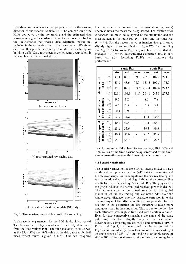
LOS direction, which is approx. perpendicular to the moving direction of the receiver vehicle Rx1. The comparison of the PDPs computed by the ray tracing and the estimated data shows a very good accordance. Nevertheless, one can find in the reconstructed ray tracing data additional power not included in the estimation, but in the measurement. We found out, that this power is coming from diffuse scattering on building walls. Only few specular components occur solely in the simulated or the estimated PDP.

(a) measurement data

(b) reconstructed ray tracing data

(c) reconstructed estimation data (SC only)

Fig. 3: Time-variant power delay profile for route Rx2. A characteristic parameter for the PDP is the delay spread. The time-variant delay spread can be directly determined from the time-variant PDP. The time-averaged value as well as the 10%, 50% and 90% value of the delay spread for both measurement routes is given in Tab. I. One can recognize,

that the simulation as well as the estimation (SC only) underestimates the measured delay spread. The relative error δ between the mean delay spread of the simulation and the measurement is for route Rx1 δsim = 15% and for route Rx2 δsim = 9%. For the reconstructed estimation data (SC only) slightly higher errors are obtained: δest = 27% for route Rx1

and δest = 19% for route Rx2. But, one has to note that the averaged PDP for the reconstructed estimation data is only based on SCs. Including DMCs will improve the performance.

route Rx1 route Rx2

sim. est. meas. sim. est. meas.

dela

y sp

read

in

ns

στ 93.0 80.1 109.5 205.5 182.2 224.7

στ

10% 63.8 48.6 78.7 151.5 109.5 176.7

στ

50% 89.1 82.3 103.2 204.4 187.6 223.6

στ

90% 129.1 108.9 141.9 264.1 243.8 275.3

azim

uth

spre

ad

at T

x in

deg

ree

σψTx

9.6 8.2 - 8.0 7.8 -

σψTx

10% 4.5 5.5 - 5.5 5.4 -

σψTx

50% 10.8 7.9 - 8.0 7.2 -

σψTx

90% 13.6 11.2 - 11.1 10.7 -

azim

uth

spre

ad

at R

x in

deg

ree

σψ Rx

40.3 47.4 - 41.1 50.1 -

σψ Rx

10% 28.2 33.6 - 36.3 39.6 -

σψ Rx

50% 40.8 50.0 - 41.3 52.6 -

σψ Rx

90% 55.1 55.7 47.8 56.2 -

Tab. 1: Summary of the characteristic average, 10%, 50% and 90%-values of the time-variant delay spread and of the time-variant azimuth spread at the transmitter and the receiver.

4.2 Spatial verification

The spatial verification of the 3-D ray tracing model is based on the azimuth power spectrum (APS) at the transmitter and the receiver array. For its computation the raw ray tracing and raw estimation data is used. Fig. 4 shows the corresponding results for route Rx1 and Fig. 5 for route Rx2. The grayscale in the graph indicates the normalized received power in decibel. The normalization is performed relative to the global maximum of the ray tracing and estimated APS over the whole travel distance. The line structure corresponds to the azimuth angle of the different multipath components. One can see that in the estimation the line structure is much more ambiguous than in the simulation. This is due to the fact that each estimated path angle is furnished with a certain variance. Even for two consecutive snapshots the angle of the same path may therefore slightly vary in the estimation. Nevertheless, comparing the estimated and simulated APS in Fig. 4 and Fig. 5, the same trend can be recognized. In Fig 4 a) one can identify distinct continuous curves starting at an angle range of 75° – 80° and ending at an angle range of -80° – 20°. Theses scattering contributions are coming from

walls, where the receiver vehicle is driving past. The same phenomenon can be recognized in Fig. 5 c). To a certain extend the estimator identifies the corresponding power as specular power, resulting in SCs with a very short live time. The APS can be characterized by its characteristic property azimuth spread. The resulting mean values and the corresponding 10%, 50%, and 90% for both routes are given in Tab. I. One can see that the simulated azimuth spread at the transmitter is slightly higher than the estimated azimuth spread. At the receiver it is the opposite situation.

5 Conclusion Verification results of the spatio-temporal behavior of an advanced 3-D ray tracing model developed at the University of Karlsruhe (TH) are presented. The ray tracing prediction shows a very good agreement along both measurement routes. It is demonstrated that the model is able to identify to a certain degree diffuse scattering components.

References

[1] K. Yu and B. Ottersten, "Models for MIMO Propagation Channels. A Review," Wiley Journal on Wireless Communications and Mobile Computing, Special Issue on Adaptive Antennas and MIMO Systems, July 2002.

[2] A.F. Molisch and F. Tufvesson, "Digital Signal Processing for Wireless Communications Handbook," chapter Multipath propagation models for broadband wireless systems, pp. 2.1–2.43, CRC Press, Dec. 2004.

[3] L. Schumacher, L.T Berger, and J. Ramiro-Moreno, "Adaptive Antenna Arrays; Trends and Applications," chapter Propagation Characterization and MIMO Channel Modeling for 3G, pp. 377–393, Springer, 2004.

[4] M.A. Jensen and J.W. Wallace, "Space-Time Signal Processing for MIMO Communications," chapter MIMO Wireless Channel Modeling and Experimental Characterization, pp. 1–39, JohnWiley & Sons, 2005.

[5] W. Wiesbeck, T. Fügen, M. Porebska, and W. Sörgel, "Channel Characterization and Modelling for MIMO and Other Recent Wireless Technologies" in Proceedings of the EUCAP 2006, Nice, France, Nov. 2006, CD-Rom.

[6] K.H. Ng, E.K. Tameh, A. Doufexi, M. Hunukumbure, and A.R. Nix, “Efficient Multielement Ray Tracing with Site-Specific Comparisons Using Measured MIMO Channel Data,” IEEE Transactions on Vehicular Technology, vol. 56, no. 3, May 2007.

[7] M.F. Catedra, J. Perez, F. Saez de Adana, and O. Gutierrez, “Efficient Ray-Tracing Techniques for Three-Dimensional Analyses of Propagation in Mobile Communications: Application to Picocell and Microcell Scenarios,” IEEE Antennas and Propagation Magazine, vol. 14, no. 2, pp. 15–28, April 1998.

[8] W. Kotterman, M. Landmann, G. Sommerkorn, R.S. Thomä, “On Diffuse and Non-Resolved Multipath Components in Directional Channel Characterisation,” XXVIIIth General Assembly of URSI, New Delhi, India, Oct. 2005.

[9] A. Richter, J. Salmi, V. Koivunen, “Distributed Scattering in Radio Channels and its Contribution to MIMO Channel Capacity,” in Proceedings EuCAP 2006, Nice, France, Nov. 2006.

[10] V. Degli-Esposti, D. Guiducci, A. deMarsi, P. Azzi, and F. Fuschini, “An Advanced Field Prediction Model Including Diffuse Scattering,” IEEE Transactions on Antennas and Propagation, vol. 52, no. 7, pp. 1717–1728, July 2004.

[11] V. Degli-Esposti, F. Fuschini, E. Vitucci, and G. Falciasecca, “Measurement and Modelling of Scattering From Buildings,” IEEE Transactions on Antennas and Propagation, vol. 55, no. 1, pp. 143–153, Jan. 2007.

[12] T. Fügen, J. Maurer, T. Kayser, and W. Wiesbeck, „Capability of 3-D Ray Tracing for Defining Parameter Sets for the Specification of Future Mobile Communications Systems,“ IEEE Transactions on Antennas and Propagation, vol. 54, no. 11, pp. 3125–3137, Nov. 2006.

[13] A. Richter, "On the Estimation of Radio Channel Parameters: Models and Algorithms (RIMAX)," Ph.D. thesis, Technische Universität Ilmenau, Ilmenau, Germany, 2005.

[14] R. Schneider, "Modellierung der Wellenausbreitung für ein bildgebendes Kfz-Radar, (in German)," Ph.D. thesis, Universität Karlsruhe (TH), Germany, 1998.

[15] C.A. Balanis, Advanced Engineering Electromagnetics, John Wiley & Sons, New York, 1989.

[16] R.J. Luebbers, “Comparison of Lossy Wedge Diffraction Coefficients with Application to Mixed Path Propagation Loss Prediction,” IEEE Transactions on Antennas and Propagation, vol. 36, no. 7, pp. 1031–1034, July 1988.

[17] G.T. Ruck, D.E. Barrick, W.D. Stuart, and C.K. Krichbaum, Radar Cross Section Handbook, Plenum Press, New York, London, 1970.

[18] J. Maurer, O. Drumm, D.L. Didascalou, and W. Wiesbeck, “A Novel Approach in the Determination of Visible Surfaces in 3D Vector Geometries for Ray-Optical Wave Propagation Modelling,” in Proceedings of the 51st IEEE Vehicular Technology Conference, VTC2000-Spring, Tokyo, May 2000, pp. 1651–1655.

[19] http://www.channelsounder.de

(a) raw ray tracing data, Tx1

(b) raw estimation data (SC only), Tx1

(c) raw ray tracing data, Rx1

(d) raw estimation data (SC only), Rx1

Fig. 4: Time-variant azimuth power spectrum at the transmitter and the receiver for route Rx1.

(a) raw ray tracing data, Tx1

(b) raw estimation data (SC only), Tx1

(c) raw ray tracing data, Rx2

(d) raw estimation data (SC only), Rx2

Fig. 5: Time-variant azimuth power spectrum at the transmitter and the receiver for route Rx2.