Application of a three-dimensional ray-tracing technique to global P, PP and Pdiff traveltime...

Application of a three-dimensional ray-tracing technique to globalP, PP and Pdiff traveltime tomography

A. Gorbatov,1,* Y. Fukao1 and S. Widiyantoro2

1 Earthquake Research Institute, University of Tokyo, Yayoi 1-1-1, Bunkyo-ku, Tokyo 113–0032, Japan2 Institut Teknologi Bandung, Jl. Ganesa 10, Bandung 40132, Indonesia

Accepted 2001 March 22. Received 2001 February 4; in original form 2000 April 7

SUMMARY

A 3-D ray-path tracing algorithm was successfully applied to global P-wave traveltimetomography. The inversion was conducted iteratively using the resultant P-wave velocitymodel as the initial model for the subsequent iteration. The LSQR method was adoptedto solve a large and sparse system of equations. This iteratively linearized inversion with3-D ray tracing increased wave-speed anomalies, located heterogeneities better and reducedsmearing as compared to those derived from a conventional one-step inversion using1-D ray tracing, although the general pattern of velocity anomalies was similar. A majordifference was found in the lowermost mantle, where the departure of a ray path fromthe great circle path tends to be in general greatest. In particular, a pronounced high-velocity anomaly develops beneath the Indian Ocean, a feature not obvious in the resultof 1-D inversion. The final P-wave velocity model was obtained by including reportedPP and Pdiff traveltime data. The addition of the PP data sharpened the images andenhanced velocity anomalies in the upper mantle, especially at latitudes above 45u of theNorthern Hemisphere. The addition of the Pdiff data sharpened and amplified velocityanomalies in the lowermost mantle in general.

Key words: inversion, ray tracing, traveltime tomography.

1 I N T R O D U C T I O N

Traveltime tomography has become a powerful tool in the

study of the Earth’s structure since the pioneering work of Aki

& Lee 1976). Later, Sengupta & Toksoz (1976) and Dziewonski

et al. (1977) extended the tomographic technique to the global

scale, showing how powerful the tomographic method is in

imaging the Earth’s large volume. Numerous global, regional

and local tomographic models have now been reported. The

inclusion of later-arrival data increased the resolution of

velocity anomaly mapping (e.g. Van der Hilst 1990; Vasco et al.

1995; Vasco & Johnson 1998). The technique of tomographic

inversion has also been developed and refined. The medium

parametrization was changed from the simple regular blocks

adopted in the early studies to irregular cells (e.g. Fukao et al.

1992; Sambridge & Gudmundsson 1998; Bijwaard et al. 1998)

or node parametrization (e.g. Zhao et al. 1992). The ray-tracing

algorithms advanced and 3-D ray-tracing techniques replaced 1-D

techniques in local tomography (e.g. Thurber 1983; Zhao et al.

1992). Recently, such techniques have also been implemented

in global-scale tomography by e.g. Bijwaard & Spakman (2000),

Gorbatov et al. (2000) and Widiyantoro et al. (2000). Further

improvement of the mantle model may be achieved through

the addition of later-arrival data, as was suggested by Vasco

et al. (1998). In the present study we incorporate a 3-D ray-

tracing algorithm into the whole-mantle tomography and

include PP and Pdiff data in the traveltime data. We present a

new P-velocity model of the whole mantle and discuss how the

effects of the incorporation of 3-D ray tracing and inclusion of

PP and Pdiff data are reflected in the new model.

2 D A T A

The arrival times of P, PP and Pdiff phases with hypocentral

parameters used in the study are selected from the carefully com-

piled and processed catalogue of global seismicity published by

Engdahl et al. (1998). This data set is based on the International

Seismological Data Centre catalogue, continuously updated with

more recent observations. The hypocentre parameters are deter-

mined using a non-linear scheme, with the inclusion of depth* Now at: Research School of Earth Sciences, the Australian National

University, Canberra ACT 0200, Australia

Geophys. J. Int. (2001) 146, 583–593

# 2001 RAS 583

at Geoscience A

ustralia on June 12, 2014http://gji.oxfordjournals.org/

Dow

nloaded from

http://gji.oxfordjournals.org/

phases (pP, pwP), and the ak135 earth model of Kennett

et al. (1995). The reported arrival times are reassociated with

seismic phases using the improved location to provide a set of

traveltimes. The variance of traveltime residuals is significantly

reduced compared with that for the original data catalogues.

The entire data set includes 7 458 864 P-wave, 155 817 PP-wave

and 129 033 Pdiff-wave arrivals. All data were corrected for

the Earth’s ellipticity and station elevations. The PP data were

also corrected for bounce-point altitude and water depth by

Engdahl et al. (1998).

For the P data the calculations of all the 3-D ray paths

are very time-consuming, hence, following the work of Van der

Hilst et al. (1997), we combined the information from event

clusters in a 1ur1ur50 km volume and station clusters in a

1ur1u region into a single summary ray path. The residual time

assigned to the summary ray was the median of all the relevant

data with residuals smaller than 5 s. Each summary ray was

composed of at least three individual rays. The resulting data

set contains 627 924 P-wave summary ray paths. The use

of summary rays reduces the uneven sampling of structure by

ray paths and the computational time required for ray tracing.

The complete data set of Pdiff and PP arrivals were used for

inversion due to the significantly smaller numbers of rays than

the P-arrival data set.

The medium was parametrized by uniform cells of 2ur2u and

19 layers down to the core–mantle boundary. The reference

1-D earth velocity model was ak135 of Kennett et al. (1995).

This earth parametrization is the same as that used by Van der

Hilst et al. (1997) so that our result may be compared directly

with their tomographic images derived by employing one-step

inversion with 1-D ray tracing.

3 M E T H O D

The fast and accurate computation of traveltimes and ray paths

in a heterogeneous earth model is essential in tomographic

studies. Several methods have been developed for such com-

putation (e.g. Farra & Madariaga 1987; Moser et al. 1992;

Nolet & Moser 1993; Snieder & Sambridge 1992) including

the pseudo-bending ray-tracing technique of Um & Thurber

(1987). Although their technique has been widely used in local

tomography, it has never been applied to global traveltime tomo-

graphy due to the relatively time-consuming algorithm and the

formalization in Cartesian coordinates. Recently, Koketsu &

Sekine (1998) extended the pseudo-bending technique developed

by Um & Thurber (1987) to the spherical earth. We implemented

this extended pseudo-bending ray-tracing algorithm in our tomo-

graphic code. This algorithm is based on the direct minimization

of traveltimes to construct propagation paths accordingly to

Fermat’s principle. The method searches iteratively the minimum-

traveltime ray path connecting the source and receiver, based

on a three-point perturbation with a straight-line approxi-

mation of ray-path segments. In the Pdiff ray-tracing pro-

cedure the medium is limited by the core–mantle boundary

(CMB) to prevent ray penetration below it. The application of

the algorithm of Koketsu & Sekine (1998) to global traveltime

tomography was successfully realized by Gorbatov et al. (2000)

and Widiyantoro et al. (2000).

The tomographic problem was solved in several iterations

where the system of linear equations was constructed based

on misfit between the observed traveltimes and those derived

through 3-D ray tracing in a laterally inhomogeneous model.

The resulting 3-D velocity model was used as the initial model

for subsequent iteration. Therefore, a set of linear equations

was defined as

Ai

aiIi

ciGi

26664

37775mi ¼

dti

�ai�1Ii�1mi�1

0

26664

37775 ,

where Ai is the matrix containing ray-segment lengths, ai and

ci are smoothness parameters, Ii is the identity matrix, Gi is

the matrix of gradient smoothing, dti is the data vector and mi

is the model vector containing the corresponding solutions

for slowness perturbations and hypocentral parameters for the

ith iteration. The term –aix1Iix1mix1 was included in order to

damp the result obtained towards the initial ak135 earth model

in each iteration. The system of linear equations described above

was solved by the LSQR method of Page & Saunders (1982).

Solving the system of linear equations takes about nine days on

a SUN Ultra 10 computer.

4 M O D E L D E V E L O P M E N T

Global tomographic images are commonly derived through

a one-step iteration procedure (e.g. Van der Hilst et al. 1997;

Bijwaard et al. 1998) and rarely through a multiple-step iteration

scheme (e.g. Fukao et al. 1992). However, the iterative strategy

should recover higher values of velocity perturbation than

those obtained from one-step inversion, especially if the 3-D

ray-bending algorithm is implemented in the inversion. For

example, seismic rays tend preferentially to pass through a high-

velocity zone in the vicinity of their great-circle paths. Such a

tendency makes it impossible in a linearized scheme to deter-

mine accurately both velocity anomalies and off-great-circle ray

paths in a one-step inversion and inherently requires iteration.

Iteration also reduces the influence of damping when a modi-

fication of the model is required by the data. The addition of

PP and Pdiff data could also enhance velocity perturbations

and improve the resolution of tomographic images. To evaluate

these influences, we compare the model with 1-D ray tracing,

the model with 3-D ray tracing and the model with 3-D ray

tracing including PP and Pdiff data.

4.1 P-wave model

The 3-D P-wave velocity model was developed using the same

parametrization as that employed by Van der Hilst et al. (1997).

However, the data set used in this study is more extensive than

the catalogue exploited by Van der Hilst et al. (1997), and this

difference could give additional differences between the images

of their model and our model. Iteration was repeated three times

to obtain the final solution. The first iteration corresponds to

an ordinary tomographic inversion with 1-D ray tracing. The

variance reduction was 49 per cent at this stage. A similar

variance reduction was obtained by Van der Hilst et al. (1997).

The subsequent runs were made by incorporating 3-D ray

tracing. The further variance reduction was 14 per cent after

the second iteration and 9 per cent (corresponding to a residual

standard deviation of 1.01 s) after the third iteration. The tomo-

graphic image after the third iteration did not differ visually

584 A. Gorbatov, Y. Fukao and S. Widiyantoro

# 2001 RAS, GJI 146, 583–593

at Geoscience A


Dow

nloaded from


from the image after the second iteration and the improve-

ment of residual standard deviation was less than 5 per cent.

Therefore, we adopted the result of the third iteration as the

final one. Although the images derived from the 1-D and 3-D

ray-tracing techniques are in general similar, they do show

differences as well. The differences include the enhancement

of velocity perturbations and the sharpening of tomographic

images.

Fig. 1(a) shows the root-mean-square (rms) velocity per-

turbation of each layer from the Earth’s surface to the CMB,

indicating that the iterative inversion scheme has gained a

significant fraction of velocity perturbation at each iteration

step. About 70 per cent of the total perturbation was achieved

by the first iteration but the remaining 30 per cent was attained

through subsequent iterations. The latter increase in velocity

perturbation is a consequence of the implementation of the 3-D

ray-tracing algorithm. Note that the velocity perturbation in

the transition region takes its relative maximum at depths of

520–660 km, just above the 660 km discontinuity (Fukao et al.

2000). Fig. 1(b) plots the spherically averaged velocity per-

turbation relative to the reference model ak135 as a function

of layer depth. In general, there is little systematic increase

or decrease of average perturbation among the first, second

and third iterations, demonstrating that the 3-D ray-tracing

algorithm does not bias the estimate of the spherically averaged

structure. A relatively large negative shift (yx0.05 per cent)

during the second and third iterations at depths of 520–660 and

1000–1200 km and a relatively large positive shift (y+0.15 per

cent) occurred at depths below 2400 km.

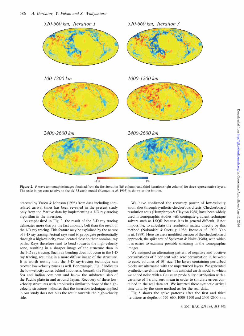
In order to see the effect of 3-D ray bending we compare the

tomographic maps after the first iteration to those after the third

iteration in the three layers at depths of 520–660, 1000–1200

and 2400–2600 km. The comparison in Fig. 2 clearly demon-

strates that the implementation of the 3-D ray tracing has

enhanced velocity perturbations and sharpened velocity contrasts

in general. Consequently, the dominance of slow anomalies at

depths of 1000–1200 km and the dominance of fast anomalies

at depths of 2400–2600 km (relative to ak135) have been

emphasized more.

Fig. 3 is a more detailed comparison of the maps at depths of

410–520 km in Asia, demonstrating again the effect of taking

into account off-great-circle ray bending, which has delineated

more sharply the fast anomaly belt associated with the sub-

ducted lithospheric slab. This point has been discussed more

fully in the tomographic study aimed at elucidating the details of

subducted slabs in the northern Pacific (Gorbatov et al. 2000).

Fig. 4 is a perturbation map at great depths (2600–2750 km)

below the Indian Ocean and shows an even more dramatic

demonstration of this effect. In this figure the tomographic map

after the third iteration (Fig. 4b) shows a pronounced high-

velocity zone extending southwards from India to the Indian

Ocean region, while that after the first iteration (1-D ray bending,

Fig. 4a) does not. This pronounced high-velocity anomaly has

not been identified by Van der Hilst et al. (1997) and Bijwaard

et al. (1998), but was imaged by Vasco & Johnson (1998), who

used a more extensive data set with the inclusion of PcP and

PKP data. Note that the solution at each iteration is always

damped towards the initial 1-D model so that the solution

should remain unchanged from the that at the first iteration

if the 3-D ray-bending effect were ignored. We attribute the

intensification of the high-velocity anomaly beneath the Indian

Ocean to the effect of ray bending in three dimensions. Of

course, the intensification of anomalies, in general, could also

be achieved by suppressing the damping parameter without

employing 3-D ray tracing. The intensification in this case

is, however, a product of allowing a larger amount of short-

wavelength perturbations and should be different from the con-

sequence of considering the effect of 3-D bending. To clarify

this point, we performed experiments on the linear (first) iteration

with reduced values of the damping factor. Fig. 4(c) shows

the result for the case with the damping parameter reduced to

a half. This underdamped solution gives a patchy image with

high-velocity spots beneath the Indian Ocean and East India.

This patchy image is, however, clearly different from the image

shown in Fig. 4(b), where the relevant high-velocity anomaly is

a broad, coherent feature with amplitudes as large as those in

the underdamped solution. The iterative non-linear inversion

has thus revealed structures usually overdamped in the linear

inversions without introducing unstable, short-wavelength per-

turbations. We have also emphasized, in conjunction with Fig. 3,

the fact that 3-D ray tracing delineates more sharply a fast

anomaly belt such as the one associated with subducted slabs

than the result of the 1-D ray tracing. This feature may be

explained by the nature of 3-D ray tracing. Actual rays tend to

propagate preferentially through a high-velocity zone located

close to their nominal ray paths. Thus, the deepest anomaly

(a)

(b)Figure 1. (a) Rms velocity perturbation values as a function of depth

for the P-wave tomographic models of Obayashi et al. (1997), van der

Hilst et al. (1997) and those obtained in the present study from the first,

second and third iterations. (b) Average perturbation values relative

to the ak135 earth model (Kennett et al. 1995) for the P-wave tomo-

graphic models obtained in this study from the first, second and third

iterations.

P, PP and Pdiff traveltime tomography 585

# 2001 RAS, GJI 146, 583–593

at Geoscience A


Dow

nloaded from


detected by Vasco & Johnson (1998) from data including core-

related arrival times has been revealed in the present study

only from the P-wave data by implementing a 3-D ray-tracing

algorithm in the inversion.

As emphasized in Fig. 3, the result of the 3-D ray tracing

delineates more sharply the fast anomaly belt than the result of

the 1-D ray tracing. This feature may be explained by the nature

of 3-D ray tracing. Actual rays tend to propagate preferentially

through a high-velocity zone located close to their nominal ray

paths. Rays therefore tend to bend towards the high-velocity

zone, resulting in a sharper image of the structure than in

the 1-D ray tracing. Such ray bending does not occur in the 1-D

ray tracing, resulting in a more diffuse image of the structure.

It is worth noting that the 3-D ray-tracing technique can

recover low-velocity zones as well. For example, Fig. 3 indicates

the low-velocity zones behind Indonesia, beneath the Philippine

Sea and Indian continent and below the subducted slab of

the Pacific plate in and around Japan. Recovery of these low-

velocity structures with amplitudes similar to those of the high-

velocity structures indicates that the inversion technique applied

in our study does not bias the result towards the high-velocity

side.

We have confirmed the recovery power of low-velocity

anomalies through synthetic checkerboard tests. Checkerboard

resolution tests (Humphreys & Clayton 1988) have been widely

used in tomographic studies with conjugate gradient technique

solvers such as LSQR because it is in general difficult, if not

impossible, to calculate the resolution matrix directly by this

method (Nakanishi & Suetsugi 1986; Inoue et al. 1990; Yao

et al. 1999). Here we use a modified version of the checkerboard

approach, the spike test of Spakman & Nolet (1988), with which

it is easier to examine possible smearing in the tomographic

images.

We assigned an alternating pattern of negative and positive

perturbations of 3 per cent with zero perturbation in between

to cubic volumes of 10u size. The layers containing perturbed

blocks are alternated with the unperturbed layers. We generated

synthetic traveltime data for this artificial earth model to which

we added noise with a Gaussian probability distribution with a

variance of 1 s and zero mean in order to simulate errors con-

tained in the real data set. We inverted these synthetic arrival

time data by the same method as for the real data.

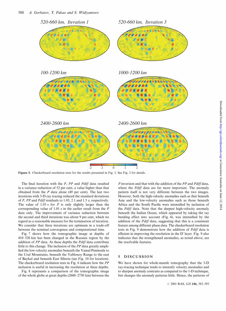
Fig. 5 shows the spike patterns after the first and third

iterations at depths of 520–660, 1000–1200 and 2400–2600 km,

-1% 1%

2400-2600 km

100-1200 km

520-660 km, Iteration 1 520-660 km, Iteration 3

1000-1200 km

2400-2600 km

Figure 2. P-wave tomographic images obtained from the first iteration (left column) and third iteration (right column) for three representative layers.

The scale in per cent relative to the ak135 earth model (Kennett et al. 1995) is shown at the bottom.


# 2001 RAS, GJI 146, 583–593

at Geoscience A


Dow

nloaded from


which can serve as a check for the patterns at the same depths

obtained from the real data (Fig. 2). A comparison of these

patterns clearly indicates that, for a given ray path coverage,

the 3-D ray tracing has recovered the intensities and patterns

of the original perturbation more satisfactorily than the 1-D

ray tracing. This comparison also demonstrates that the 3-D

ray tracing does not bias the resultant pattern systematically

towards either the high- or the low-velocity side.

4.2 Addition of PP and Pdiff data

Exploitation of additional data could increase the resolution

of tomographic images and introduce new information into

the inversion results. PP seismic data were successfully included

previously (e.g. Van der Hilst 1990; Vasco et al. 1995; Vasco &

Johnson 1998), although the reading of PP arrivals is inherently

more difficult than first-arrival reading, in part because PP is

a later phase and in part because it is shifted in phase by p /2

relative to P (Choy & Richards 1975; Darragh 1985; Woodward

& Masters 1991; Paulseen & Stutzman 1996). No attempt has

been made so far to incorporate reported Pdiff data into tomo-

graphic inversions. In an attempt to improve our tomographic

image we will add the PP and Pdiff arrival times to the P data,

all from the newly compiled data set of Engdahl et al. (1998).

-10˚

0˚

10˚

20˚

30˚

40˚

50˚

(a)

410-520 km

70˚ 80˚ 90˚ 100˚ 110˚ 120˚ 130˚ 140˚ 150˚-10˚

0˚

10˚

20˚

30˚

40˚

50˚

-1% -0.5 0.0 0.5 1%

(b)

Figure 3. Comparison of tomographic images obtained from the first

(a) and third (b) iterations for Asia at the 410–520 km layer. Note that

the third non-linear iteration produces a sharper image than the first

iteration corresponding to the conventional linearized tomography.

The scale in per cent relative to the ak135 earth model (Kennett et al.

1995) is shown at the bottom.

-30˚

-20˚

-10˚

0˚

10˚

20˚

30˚

a)

2750 km

-30˚

-20˚

-10˚

0˚

10˚

20˚

30˚

b)

20˚ 30˚ 40˚ 50˚ 60˚ 70˚ 80˚ 90˚ 100˚ 110˚ 120˚-30˚

-20˚

-10˚

0˚

10˚

20˚

30˚

-0.5% 0.5%

c)

(a)

(b)

(c)

Figure 4. Results of tomographic inversion at a depth of 2750 km

below the Indian Ocean (a) from the first linear iteration, (b) from the

third non-linear iteration, and (c) from the first linear iteration with

the damping parameter decreased by a factor of two (see text for

explanation).


# 2001 RAS, GJI 146, 583–593

at Geoscience A


Dow

nloaded from


The final iteration with the P, PP and Pdiff data resulted

in a variance reduction of 52 per cent, a value higher than that

obtained from the P data alone (49 per cent). The last two

iterations with 3-D ray tracing reduced the standard deviations

of P, PP and Pdiff residuals to 1.03, 2.1 and 1.5 s, respectively.

The value of 1.03 s for P is only slightly larger than the

corresponding value of 1.01 s in the earlier result from the P

data only. The improvement of variance reduction between

the second and third iterations was about 9 per cent, which we

regard as a reasonable measure for the termination of iteration.

We consider that three iterations are optimum in a trade-off

between the nominal convergence and computational time.

Fig. 7 shows how the tomographic image at depths of

410–520 km has been changed in the Russian region by the

addition of PP data. At these depths the Pdiff data contribute

little to this change. The inclusion of the PP data greatly ampli-

fied the low-velocity anomalies beneath the Yamal Peninsula to

the Ural Mountains, beneath the Yablonoy Range to the east

of Baykal and beneath East Siberia (see Fig. 10 for location).

The checkerboard resolution tests in Fig. 6 indicate how the PP

inclusion is useful in increasing the resolution at these depths.

Fig. 8 represents a comparison of the tomographic image

of the whole globe at great depths (2600–2750 km) between the

P inversion and that with the addition of the PP and Pdiff data,

where the Pdiff data are far more important. The anomaly

pattern itself is not very different between the two images.

However, both the high-velocity anomalies such as that beneath

Asia and the low-velocity anomalies such as those beneath

Africa and the South Pacific were intensified by inclusion of

the Pdiff data. Note that the deepest high-velocity anomaly

beneath the Indian Ocean, which appeared by taking the ray

bending effect into account (Fig. 4), was intensified by the

addition of the Pdiff data, suggesting that this is a consistent

feature among different phase data. The checkerboard resolution

tests in Fig. 9 demonstrate how the addition of Pdiff data is

efficient in improving the resolution in the Dk layer. Fig. 9 also

indicates that the strengthened anomalies, as noted above, are

the resolvable features.

5 D I S C U S S I O N

We have shown for whole-mantle tomography that the 3-D

ray-tracing technique tends to intensify velocity anomalies and

to sharpen anomaly contrasts as compared to the 1-D technique,

but changes the anomaly patterns little. Hence, the patterns of

-2 -1 0 1 2

2400-2600 km

100-1200 km

520-660 km, Iteration 1 520-660 km, Iteration 3

1000-1200 km

2400-2600 km

Figure 5. Checkerboard resolution tests for the results presented in Fig. 2. See Fig. 2 for details.


# 2001 RAS, GJI 146, 583–593

at Geoscience A


Dow

nloaded from


our tomographic image are not, in general, very different from

those of previous studies (e.g. Fukao et al. 1992; Van der Hilst

et al. 1997; Bijwaard et al. 1998; Vasco & Johnson 1998). The

synthetic recovery tests for given structures have confirmed

that the application of the 3-D technique, in general, reduces

smearing in tomograms. The increase in velocity perturbation

with increasing number of iterations is clearly demonstrated

in Fig. 1. Also shown in this figure are the rms variations for

the two tomographic models of Van der Hilst et al. (1997) and

Obayashi et al. (1997) (see Fukao et al. 2000). All the curves

show a similar trend. The rms perturbation has its maximum in

the uppermost mantle, decreases rapidly with increasing depth

down to 400 km and then increases to take a relative maximum

at a depth of 500 km. The perturbation then decreases relatively

rapidly down to a depth of 1000 km. The perturbation curve in

the depth range 1000–2400 km is fairly flat with a broad mini-

mum at approximately 2000 km. At depths below 2400 km

the perturbation begins to increase sharply. The contrast in the

behaviour of the rms variation across a depth of 1000 km has

been pointed out by Tanimoto (1990), Montagner (1994) and

Wen & Anderson (1995). The above trend is common in all

the curves in Fig. 1, which provides support for the earlier

conclusion that the non-linear inversion with 3-D ray tracing

does not alter the general features of the tomographic image

of the Earth obtained by a linearized inversion with 1-D ray

tracing (Van der Hilst et al. 1997) or a non-linear inversion with

1-D ray tracing (Obayashi et al. 1997). It may be noted that the

models from the non-linear inversions, either 3-D or 1-D ray

tracing, show similar rms variations in terms of not only the

trend but also the amplitude, although a precise comparison is

meaningless because of many differences in methodology.

The addition of the PP data has improved the resolution in

the upper mantle, especially in the Russian region (Fig. 6). For

example, on the tomographic map at depths of 410–520 km in

Fig. 7, the PP addition has revealed the low-velocity anomaly

beneath the Ural Range that separates the high-velocity anomaly

20˚

30˚

40˚

50˚

30˚

40˚

20˚

30˚

40˚

50˚

30˚

40˚

410-520 km

20˚

30˚

40˚

50˚

30˚

40˚

20˚

30˚

40˚

50˚

60˚

70˚

80˚

90˚

100˚

110˚

120˚

130˚

30˚

30˚40˚

-2% 2%

410-520 km

(a)

(b)

Figure 6. Checkerboard resolution tests for the tomographic images presented in the Fig. 7. The inclusion of PP-wave arrival times (b) increases

resolution in the upper mantle.


# 2001 RAS, GJI 146, 583–593

at Geoscience A


Dow

nloaded from


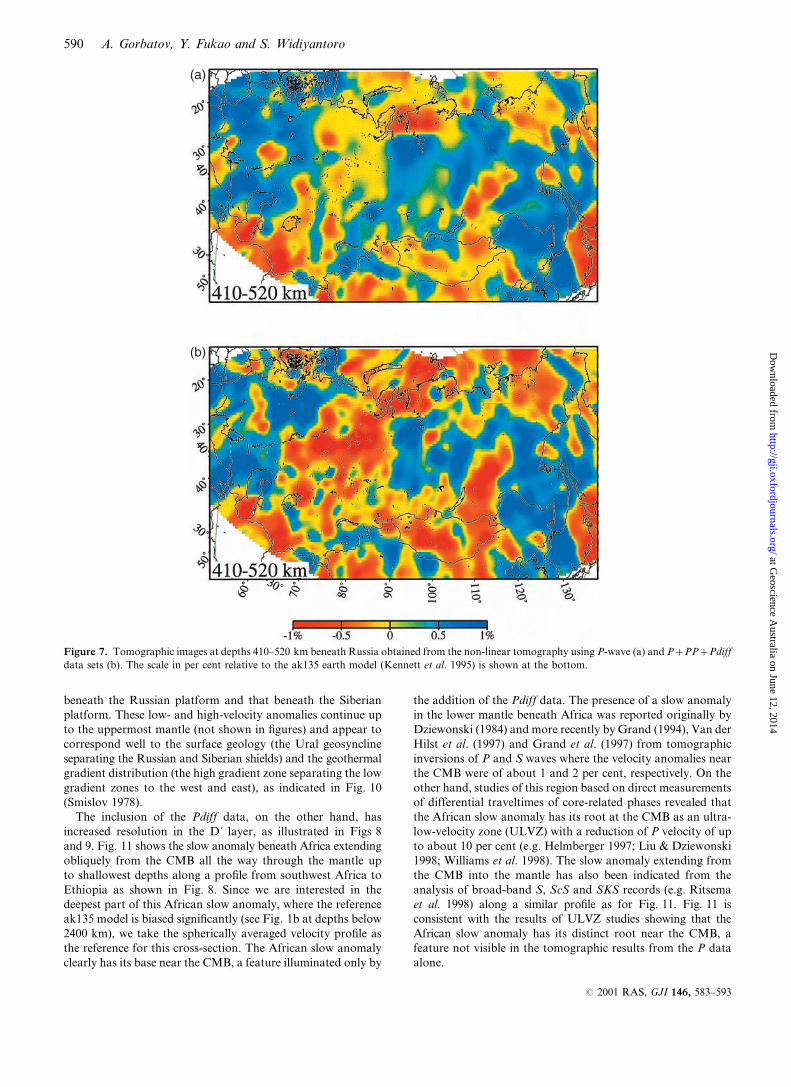
beneath the Russian platform and that beneath the Siberian

platform. These low- and high-velocity anomalies continue up

to the uppermost mantle (not shown in figures) and appear to

correspond well to the surface geology (the Ural geosyncline

separating the Russian and Siberian shields) and the geothermal

gradient distribution (the high gradient zone separating the low

gradient zones to the west and east), as indicated in Fig. 10

(Smislov 1978).

The inclusion of the Pdiff data, on the other hand, has

increased resolution in the Dk layer, as illustrated in Figs 8

and 9. Fig. 11 shows the slow anomaly beneath Africa extending

obliquely from the CMB all the way through the mantle up

to shallowest depths along a profile from southwest Africa to

Ethiopia as shown in Fig. 8. Since we are interested in the

deepest part of this African slow anomaly, where the reference

ak135 model is biased significantly (see Fig. 1b at depths below

2400 km), we take the spherically averaged velocity profile as

the reference for this cross-section. The African slow anomaly

clearly has its base near the CMB, a feature illuminated only by

the addition of the Pdiff data. The presence of a slow anomaly

in the lower mantle beneath Africa was reported originally by

Dziewonski (1984) and more recently by Grand (1994), Van der

Hilst et al. (1997) and Grand et al. (1997) from tomographic

inversions of P and S waves where the velocity anomalies near

the CMB were of about 1 and 2 per cent, respectively. On the

other hand, studies of this region based on direct measurements

of differential traveltimes of core-related phases revealed that

the African slow anomaly has its root at the CMB as an ultra-

low-velocity zone (ULVZ) with a reduction of P velocity of up

to about 10 per cent (e.g. Helmberger 1997; Liu & Dziewonski

1998; Williams et al. 1998). The slow anomaly extending from

the CMB into the mantle has also been indicated from the

analysis of broad-band S, ScS and SKS records (e.g. Ritsema

et al. 1998) along a similar profile as for Fig. 11. Fig. 11 is

consistent with the results of ULVZ studies showing that the

African slow anomaly has its distinct root near the CMB, a

feature not visible in the tomographic results from the P data

alone.

(a)

(b)

Figure 7. Tomographic images at depths 410–520 km beneath Russia obtained from the non-linear tomography using P-wave (a) and P+PP+Pdiff

data sets (b). The scale in per cent relative to the ak135 earth model (Kennett et al. 1995) is shown at the bottom.


# 2001 RAS, GJI 146, 583–593

at Geoscience A


Dow

nloaded from


6 C O N C L U S I O N S

Implementation of a 3-D ray-tracing technique to the whole-

mantle P-wave traveltime tomography shows that the pattern

of the tomographic image does not, in general, differ signifi-

cantly from that obtained from the conventional tomography

with 1-D ray tracing. The incorporation of 3-D ray tracing,

however, enhanced velocity anomalies and sharpened velocity

contrasts appreciably. A typical example is found beneath

the Indian Ocean in the Dk layer, where a prominent high-

velocity anomaly has appeared only by implementing this

algorithm. The addition of later seismic phases such as PP and

Pdiff has increased resolution in the upper and lowermost

mantle, respectively. In particular, a remarkable improvement

of resolution is achieved beneath Siberia due to the inclusion of

PP traveltimes, where a pair of high- and low-velocity zones

has appeared in the upper mantle that correlates well with

the Siberian shield and the Ural Range, and with low and high

heat flow regions, respectively. The inclusion of Pdiff data, on

the other hand, has increased significantly the amplitudes of

anomalies in the lowermost mantle. An example is the African

low-velocity anomaly with its roots just above the CMB

underneath southwest Africa.

-1% 1%

2600-2750 km

P+PP+Pdiff

A

A’

2600-2750 km

P

Figure 8. Tomographic images for the inversions using P (shown at

the top) and P+PP+Pdiff (shown at the bottom) data sets at the depth

range 2600–2750 km. Black solid line AAk denotes the location of the

cross-section presented in Fig. 11. Grey areas show the zones without

ray coverage. The scale in per cent relative to the ak135 earth model

(Kennett et al. 1995) is shown at the bottom.

-2 -1 0 1 2

2600-2750 km

P+PP+Pdiff

2600-2750 km

P

Figure 9. Checkerboard resolution tests for the tomographic models

presented in Fig. 8. See Fig. 8 for explanation.

2800km

410km660km

A A’

2800km

410km660km

-1% +1%Figure 11. Cross-sections of the tomographic models from the P

(shown at the top) and P+PP+Pdiff data (shown at the bottom)

across the African slow anomaly. See Fig. 8 for location. The scale in

per cent relative to the spherically averaged velocity profile of the final

model is shown at the bottom.


# 2001 RAS, GJI 146, 583–593

at Geoscience A


Dow

nloaded from


A C K N O W L E D G M E N T S

We thank B. L. N. Kennett and M. Obayashi for useful sug-

gestions and discussions. We are very grateful to E. R. Engdahl,

R. D. van der Hilst and R. Buland for the updated version

of their hypocentre and phase global data set. G. Nolet and

J. Virieux provided us with helpful comments and suggestions

that improved the manuscript.

R E F E R E N C E S

Aki, K. & Lee, W.H.K., 1976. Determination of three-dimensional

velocity anomalies under a seismic array using first P arrival times

from local earthquakes, 1, A homogeneous initial model, J. geophys.

Res., 81, 4381–4399.

Bijwaard, H. & Spakman, W., 2000. Non-linear global P-wave

tomography by iterated linearized inversion, Geophys. J. Int., 141,

71–82.

Bijwaard, H., Spakman, W. & Engdahl, E.R., 1998. Closing the gap

between regional and global travel-time tomography, J. geophys.

Res., 103, 30 055–30 078.

Choy, G.L. & Richards, P., 1975. Pulse distortion and Hilbert

transformation in multiply reflected and refracted body waves,

Bull. seism. Soc. Am., 65, 55–70.

Darragh, R.B., 1985. Mapping of upper-mantle structure from

differential (PP-P) travel-time residuals, Phys. Earth planet Inter.,

41, 6–17.

Dziewonski, A.M., 1984. Mapping the lower mantle: determination

of lateral heterogeneity in P velocity up to degree and order 6,

J. geophys. Res., 89, 5929–5925.

Dziewonski, A.M., Hager, B.H. & O’Connell, R.J., 1977. Large-scale

heterogeneities in the lower mantle, J. geophys. Res., 82, 239–255.

Engdahl, E.R., Van der Hilst, R.D. & Buland, R.P., 1998. Global

teleseismic earthquake relocation with improved travel times

and procedures for depth determination, Bull. seism. Soc. Am., 88,

722–743.

Farra, V. & Madariaga, R., 1987. Seismic waveform modeling in

heterogeneous media by ray perturbation theory, J. geophys. Res., 92,

2697–2712.

Fukao, Y., Obayashi, M., Inoue, H. & Nenbai, M., 1992. Subducting

slabs stagnant in the mantle transition zone, J. geophys. Res., 97,

4809–4822.

Fukao, Y., Widiyantoro, S. & Obayashi, M., 2000. Stagnant slabs in

the upper and lower mantle transition region, Rev. Geophys., in press.

Gorbatov, A., Widiyantoro, S., Fukao, Y. & Gordeev, E., 2000.

Signature of remnant slabs in the North Pacific from P-wave

tomography, Geophys. J. Int., 142, 27–36.

Grand, S.P., 1994. Mantle shear structure beneath the Americas and

the surrounding oceans, J. geophys. Res., 99, 11 591–11 621.

Grand, S.P., Van der Hilst, R.D. & Widiyantoro, S., 1997. Global

seismic tomography: a snapshot of convection in the Earth, Geol.

Soc. Am. Today, 7, 1–7.

Helmberger, D.V., 1997. Extremes in CMB structure beneath Europe

and Africa, EOS Trans. Am. geophys. Un., Fall Mtng, U11A-6, F1.

Humphreys, E. & Clayton, R.W., 1988. Adaption of back projection

tomography to seismic travel time problems, J. geophys. Res., 93,

1073–1085.

Inoue, H., Fukao, Y., Tanabe, K. & Ogata, Y., 1990. Whole mantle

P-wave travel time tomography, Phys. Earth. planet. Inter., 59,

294–328.

Kennett, B.L.N., Engdahl, E.R. & Buland, R., 1995. Constraints on

seismic velocities in the Earth from traveltimes, Geophys. J. Int., 122,

108–124.

Koketsu, K. & Sekine, S., 1998. Pseudo-bending method for

three-dimensional seismic ray tracing in a spherical earth with

discontinuities, Geophys. J. Int., 132, 339–346.

Liu, X.-F. & Dziewonski, 1998. Global analysis of shear wave velocity

anomalies in the lowermost mantle, in The Core–Mantle Boundary

Region, eds Gurnis, M., Wysession, M., Knittle, E. & Buffett, B.A.,

Am. geophys. Un. Geodyn. Ser., 28, 21–36.

Montagner, J.-P., 1994. Can seismology tell us anything about

convection in the mantle, Rev. Geophys., 32, 115–137.

Moser, T.J., Nolet, G. & Snieder, R., 1992. Ray bending revised, Bull.

seism. Soc. Am., 82, 259–288.

Nakanishi, I. & Suetsugi, D., 1986. Resolution matrix calculated by a

tomographic inversion method, J. Phys. Earth, 34, 95–99.

Nolet, G. & Moser, T.J., 1993. Teleseismic delay times in a 3-D Earth

and a new look at the S discrepancy, Geophys. J. Int., 114, 185–195.

Obayashi, M., Sakurai, T. & Fukao, Y., 1997. Comparison of recent

tomographic models, in Int. Symp. New Images of the Earth’s Interior

Through Long-Term Ocean-Floor Observations, Vol. 29, Tokyo.

Page, C.C. & Saunders, M.A., 1982. LSQR: an algorithm for sparse

linear equations and sparse least squares, ACM Trans. Math. Soft.,

8, 43–71.

Paulseen, H. & Stutzman, E., 1996. On PP-P differential travel-time

measurements, Geophys. Res. Lett., 23, 1833–1836.

10 15 20 25 40

C/1000 m

64

60

56

52

48

44

40

174144967248302418

O

Siberiaplatform

Russianplatform

Ura

lR

ange

Yamal pen.

Yablonoy Ra.

Bay

kal l

ake

Figure 10. Schematic map of the heat flow distribution over the former URSS, recompiled from Smislov (1978).


# 2001 RAS, GJI 146, 583–593

at Geoscience A


Dow

nloaded from


Ritsema, J., Ni, S., Helmberger, D.V. & Crotwell, H.P., 1998.

Evidence for strong shear velocity reductions and velocity gradients

in the lower mantle beneath Africa, Geophys. Res. Lett., 25,

4245–4248.

Sambridge, M. & Gudmundsson, O., 1998. Tomographic systems of

equations with irregular cells, J. geophys. Res., 103, 773–781.

Sengupta, M. & Toksoz, M.N., 1976. Three-dimensional model of

seismic velocity variation in the Earth’s mantle, Geophys. Res. Lett.,

3, 84–86.

Smislov, A.A., 1978. The Map of the Geothermal Flow of the Earth

Crust of the USSR, VSEGEI, MINGEO USSR, Moscow.

Snieder, R. & Sambridge, M., 1992. Ray perturbation theory for

traveltimes and ray paths in 3-D heterogeneous media, Geophys. J.

Int., 109, 294–322.

Spakman, W. & Nolet, G., 1988. Imaging algorithms, accuracy and

resolution in delay time tomography, in Mathematical Geophysics,

pp. 155–187, eds Vlaar, N.J. et al., D. Reidel, Norwell, MA.

Tanimoto, T., 1990. Predominance of large-scale heterogeneity and

the shift of velocity anomalies between the upper and lower mantle,

J. Phys. Earth, 38, 493–509.

Thurber, C.H., 1983. Earthquake locations and three-dimensional

crustal structure in the Coyote Lake area, central California,

J. geophys. Res., 88, 8226–8236.

Um, J. & Thurber, C., 1987. A fast algorithm for two-point seismic ray

tracing, Bull. seism. Soc. Am., 77, 972–986.

Van der Hilst, R.D., 1990. Tomography with P, PP and pP delay-time

data and the three-dimensional mantle structure below the Caribbean

region, PhD thesis, Utrecht University, Utrecht, the Netherlands.

Van der Hilst, R.D., Widiyantoro, S. & Engdahl, E.R., 1997. Evidence

for deep mantle circulation from global tomography, Nature, 386,

578–584.

Vasco, D.W. & Johnson, L.R., 1998. Whole Earth structure estimated

from seismic arrival times, J. geophys. Res., 103, 2633–2671.

Vasco, D.W., Johnson, L.R. & Pulliam, R.J., 1995. Lateral variations

in mantle velocity structure and discontinuities determined from P,

PP, S, SS, and SS-SdS travel time residuals, J. geophys. Res., 100,

24 037–24 059.

Wen, L. & Anderson, D.L., 1995. The fate of slabs inferred from

seismic tomography and 130 million years of subduction, Earth planet.

Sci. Lett., 133, 185–198.

Widiyantoro, S., Gorbatov, A., Kennett, B.L.N. & Fukao, Y., 2000.

Improving global shear wave traveltime tomography using three-

dimensional ray tracing and iterative inversion, Geophys. J. Int., 141,

747–758.

Williams, Q., Revenaugh, J. & Garnero, E., 1998. A correlation

between ultra-low basal velocities in the mantle and hot spots,

Science, 281, 546–549.

Woodward, R.L. & Masters, G., 1991. Global upper mantle structure

from long-period differential travel times, J. geophys. Res., 96,

6351–6377.

Yao, Z.S., Roberts, R.G. & Tryggvason, A., 1999. Calculating

resolution and covariance matrices for seismic tomography with

the LSQR method, Geophys. J. Int., 138, 886–894.

Zhao, D., Hasegawa, A. & Horiuchi, S., 1992. Tomographic imaging

of P and S wave velocity structure beneath northeastern Japan,

J. geophys. Res., 97, 19 909–19 928.


# 2001 RAS, GJI 146, 583–593

at Geoscience A


Dow

nloaded from


Application of a three-dimensional ray-tracing technique to global P, PP and Pdiff traveltime...

Documents

Transcript of Application of a three-dimensional ray-tracing technique to global P, PP and Pdiff traveltime...