
Hybrid tomography for conductivity imaging
30
arXiv:1112.2958v2 [physics.med-ph] 16 Jan 2012 Hybrid tomography for conductivity imaging Thomas Widlak 1 , Otmar Scherzer 1,2 1 Computational Science Center, University of Vienna, Nordbergstr. 15, A-1090 Vienna, Austria 2 RICAM, Austrian Academy of Sciences, Altenberger Str. 69, A-4040 Linz, Austria December 13, 2011 Abstract Hybrid imaging techniques utilize couplings of physical modalities – they are called hybrid, because, typically, the excitation and measurement quantities belong to dif- ferent modalities. Recently there has been an enormous research interest in this area because these methods promise very high resolution. In this paper we give a review on hybrid tomography methods for electrical conductivity imaging. The reviewed imag- ing methods utilize couplings between electric, magnetic and ultrasound modalities. By this it is possible to perform high-resolution electrical impedance imaging and to overcome the low-resolution problem of electric impedance tomography. 1 Introduction The spatially varying electrical conductivity, denoted by σ = σ(x) in the following, provides important functional information for diagnostic imaging – it is an appropriate parameter for distinguishing between malignant and benignant tissue [23, 28, 38, 39, 42, 55, 65, 82, 89, 103]. Although almost never stated explicitly, but very relevant for this work, the conductivity is frequency dependent, that is, σ = σ(ω). The dependence on ω is typically neglected, since the imaging devices operate at a fixed frequency. However, one should be aware that different image devices record conductivities in different frequency regimes. In figures 1a and 1b, respectively, the specific values for σ in healthy and malignant tissues are plotted, and it can be observed that cancerous tissue reveals a higher conductivity, in general. (a) Low frequency contrast of σ [28, 42, 89] (b) Radio-frequency contrast of σ [38] Figure 1: Contrast of conductivity in biological tissue The standard approach for determining the electrical conductivity is Electrical Impedance Tomography (EIT). This approach is based on the electrostatic equation: ∇ · (σ∇u)=0 , (1.1) 1
-
Upload
independent -
Category
Documents
-
view
2 -
download
0
Transcript of Hybrid tomography for conductivity imaging
arX
iv:1
112.
2958
v2 [
phys
ics.
med
-ph]
16
Jan
2012
Hybrid tomography for conductivity imaging
Thomas Widlak1, Otmar Scherzer1,2
1 Computational Science Center, University of Vienna, Nordbergstr. 15, A-1090 Vienna, Austria2 RICAM, Austrian Academy of Sciences, Altenberger Str. 69, A-4040 Linz, Austria
December 13, 2011
Abstract
Hybrid imaging techniques utilize couplings of physical modalities – they are called
hybrid, because, typically, the excitation and measurement quantities belong to dif-
ferent modalities. Recently there has been an enormous research interest in this area
because these methods promise very high resolution. In this paper we give a review on
hybrid tomography methods for electrical conductivity imaging. The reviewed imag-
ing methods utilize couplings between electric, magnetic and ultrasound modalities.
By this it is possible to perform high-resolution electrical impedance imaging and to
overcome the low-resolution problem of electric impedance tomography.
1 Introduction
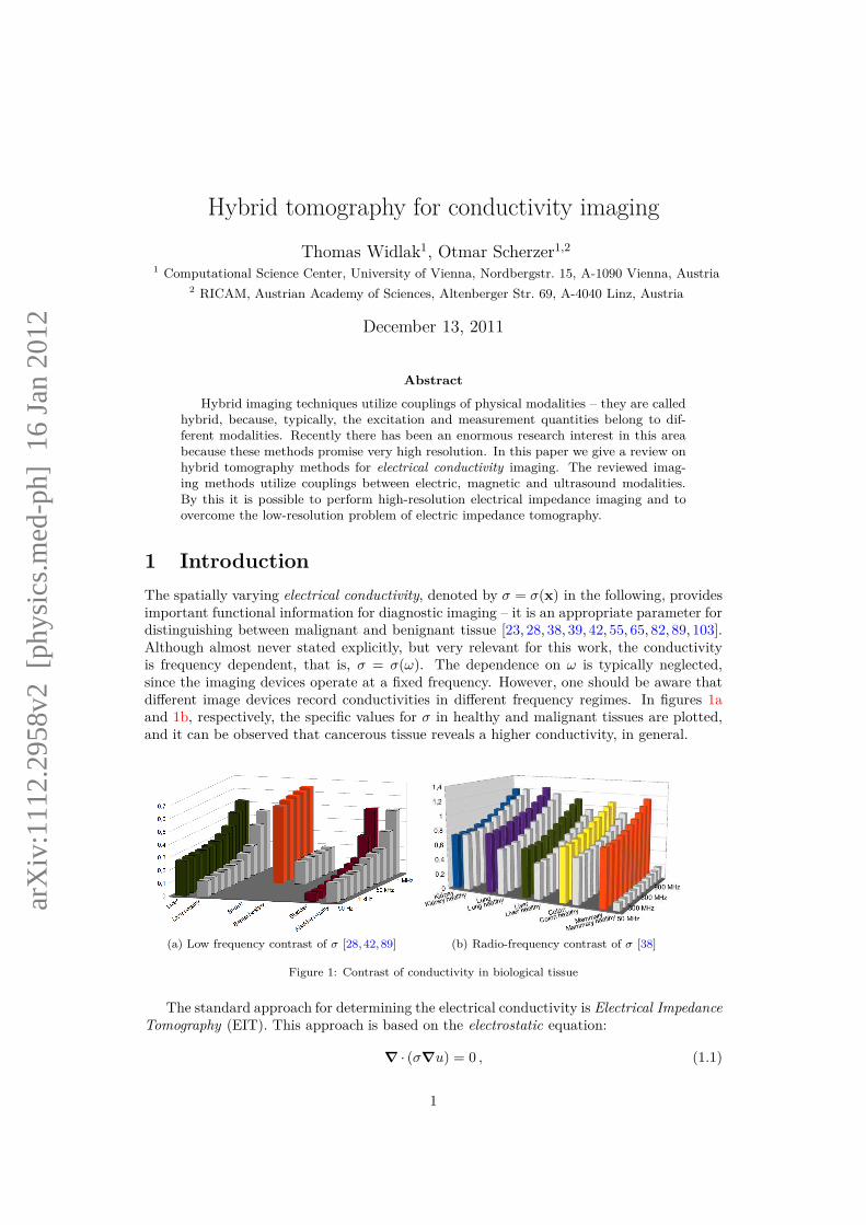
The spatially varying electrical conductivity, denoted by σ = σ(x) in the following, providesimportant functional information for diagnostic imaging – it is an appropriate parameter fordistinguishing between malignant and benignant tissue [23, 28, 38, 39, 42, 55, 65, 82, 89, 103].Although almost never stated explicitly, but very relevant for this work, the conductivityis frequency dependent, that is, σ = σ(ω). The dependence on ω is typically neglected,since the imaging devices operate at a fixed frequency. However, one should be aware thatdifferent image devices record conductivities in different frequency regimes. In figures 1aand 1b, respectively, the specific values for σ in healthy and malignant tissues are plotted,and it can be observed that cancerous tissue reveals a higher conductivity, in general.
(a) Low frequency contrast of σ [28, 42, 89] (b) Radio-frequency contrast of σ [38]
Figure 1: Contrast of conductivity in biological tissue
The standard approach for determining the electrical conductivity is Electrical ImpedanceTomography (EIT). This approach is based on the electrostatic equation:
∇ · (σ∇u) = 0 , (1.1)
1

2 T. WIDLAK AND O. SCHERZER
which describe the relation between the conductivity σ and the electrostatic potential u =u(x). For imaging, EIT is realized by injecting series of currents at a certain frequencyω on the surface ∂Ω of the probe and measuring the according series of voltages there.In mathematical terms the EIT problem accounts for computing σ from the Dirichlet-to-Neumann mapping Λσ : f 7→ g, which relates the components of all possible pairs (f = u|∂Ω,g = σ ∂nu|∂Ω).
Precursors of EIT were for geological prospecting [35, 86]. Current applications of EITare in geology [2, 76, 80], but the applications in non-destructive testing for industry are ofgrowing importance [96]. There has been considerable effort in adapting EIT for medicalapplications [13, 18].
In mathematical terms the EIT problem has been formulated first in 1980 by Calderón[16]. Uniqueness and stability have been studied extensively (see e.g. [1, 15, 92]).1 Therecovery of the electrical conductivity from the Dirichlet-to-Neumann map is heavily ill-conditioned, the modulus of continuity is at most logarithmic [3,64]. This result is consistentwith the abilities of classical EIT to differentiate between conductors and insulators ingeological prospecting (see table 1). On the other hand, the material differences in humanand biological tissues are smaller, and logarithmic stability in this case guarantees only verylow resolution.
tissue type/material conductivity σskin 2 · 10−3 S/mblood 6 · 10−1 S/mfat 4 · 10−2 S/mliver 1, 4 · 10−1 S/mcopper 6 · 107 S/mgranite 10−5 S/m
Table 1: Conductivities of different type of tissue or materials, respectively, at typical frequencies [63, Tab.7.3], [20, Tab. 9.11], [74]
Recently, coupled Physics imaging methods (this is another name for hybrid imaging,which is more self explaining), have been developed, which can serve as alternatives forestimating the electrical conductivity. Passive coupled Physics electrical impedance imagingutilizes that electrical currents in the interior of a probe manifest themselves in differentmodality. In contrast, active coupled Physics imaging is by local excitement of the tissuesample. Mathematically, in most cases, coupled Physics imaging decouples into two inverseproblems, which, in total, are expected to better well conditioned than the EIT problem.Coupled Physics imaging led to a series of new results in inverse problems theory (see [9,46]).
Coupled Physics imaging should not be confused with multi-modal imaging (actually bothare sometimes called hybrid imaging), which is based on co-registering or fusing images ofdifferent modalities. In contrast to multi-modal imaging, the techniques described here, allinvolve interaction of physical processes, and therefore they have to use the correct modelingof the physics and chemistry involved.
In this paper we survey mathematical models for coupled Physics electrical impedanceimaging. We provide the principal mathematical modeling tools in section 2, which arevarious electromagnetic equations in different frequency ranges, basic equations of acoustics,and basics of magnetic resonance imaging (MRI). Based on this we derive mathematicalmodels for multi Physics imaging models in section 4. Bibliographic references are provided,covering experimental and mathematical research.
1 The first step to prove unique recovery of σ from Λσ for smooth conductivities, was the result in [90].Now, there exist results for less regular conductivities (see the references in [1, 14.2.1.7] and [92, 6.1]).For planar domains, one even has uniqueness for L∞-conductivities [8].

HYBRID TOMOGRAPHY FOR CONDUCTIVITY IMAGING 3
symbol name unitρ(x) electrical charge density As/m3
E(x, t) electrical field strength V/mH(x, t) magnetic field strength A/mD(x, t) electrical displacement field As/m2
B(x, t) magnetic flux density Vs/m2 = TJ(x, t) electrical current density A/m2
σ(x, ω) electrical conductivity A/Vm = 1/Ωm = S/mε(x, ω) electrical permittivity As/Vm=F/mµ(x, ω) magnetic permeability Vs/Am=H/m
Table 2: Electromagnetic quantities
2 Background
In the following we provide basic background information on mathematical equations inElectromagnetism, Acoustics, and Magnetic Resonance Imaging (MRI). This overview isrequired to survey coupled Physics impedance imaging techniques in section 4.
2.1 Electromagnetic theory
We use as a starting point Maxwell’s equations, which couple the physical quantities sum-marized in table 2.
Maxwell’s equations
are the basic formulas of electromagnetism, and read as follows (see for instance [37]):
∇ × E = −∂B
∂t, ∇ · D = ρ ,
∇ × H = J +∂D
∂t, ∇ · B = 0.
(2.1)
For later reference, we recall two equations relating the fields E, B with the charge densityρ and the current density J:
• First, the fields E and B act on free charges and electrical currents by the Lorentzforce. The force per unit volume is given by (see [37, (5.12)]):
f(x, t) = ρE + J × B. (2.2)
• Secondly, the work of the electromagnetic fields per unit volume and unit time is thepower density [37, (6.103)], which in formulas expresses as
H(x, t) = J · E. (2.3)
In electromagnetism, in many applications, it is observed that the vector fields in (2.1)have the form
E(x, t) =(
Ek0 (x) cos(ωt+ ϕk
E))
k=1,2,3,
B(x, t) =(
Bk0 (x) cos(ωt+ ϕk
B))
k=1,2,3,
D(x, t) =(
Dk0 (x) cos(ωt+ ϕk
D))
k=1,2,3,
H(x, t) =(
Bk0 (x) cos(ωt+ ϕk
H))
k=1,2,3,
J(x, t) =(
Jk0 (x) cos(ωt+ ϕk
J ))
k=1,2,3.
4 T. WIDLAK AND O. SCHERZER
Often the complex phasors
E(x) =(
Ek0 (x) eiωϕk
E
)
k=1,2,3,
B(x) =(
Bk0 (x) eiωϕk
B
)
k=1,2,3,
D(x) =(
Dk0 (x) eiωϕk
D
)
k=1,2,3,
H(x) =(
Hk0 (x) eiωϕk
H
)
k=1,2,3,
J(x) =(
Jk0 (x) eiωϕk
J
)
k=1,2,3,
are used to rewrite (2.1) into a system of equations for complex functions without time-differentiation:
∇ × E = −iω B , ∇ · D = ρ ,
∇ × H = J + iωD , ∇ · B = 0.(2.4)
The real physical fields, which are time-dependent, can be uniquely recovered from thecomplex but time-independent phasors via the formula E(x, t) = Re
(
E(x) · eiωt)
. We donot distinguish between E(x, t) and E(x) in the following.
It is common to assume that the three dimensional time-dependent vector fields E =E(x, t), D = D(x, t), B = B(x, t) and H = H(x, t) and J = J(x, t) satisfy functionalrelations [37, I.4]:
J = J(E,B) , D = D(E,B) , H = H(E,B) . (2.5)
For a variety of materials, including biological tissue, the material relations (2.5) are rathersimple: In these linear media, the fields are be connected by linear material relations
J = σE . D = εE , B = µH . (2.6)
By these relations, the material parameters σ = σ(x, t), ε = ε(x, t) and µ = µ(x, t) aredefined. They are in general matrix-valued functions, depending on space and time.
For biological tissue, the parameters conductivity and permittivity parameters have beeninvestigated thoroughly [23,82]. These parameters are considered mostly as scalar, althoughrarely also anisotropy is investigated. A salient feature of the electrical parameters in tissueis their dispersion: That is, σ = σ(x, ω) and ε = ε(x, ω) are functions of the frequency ωof the electrical field, respectively [23, 82]. However, as already stated above, this feature ismostly neglected, since the experiments usually operate in a fixed frequency regime.
In biological tissue the electrical conductivity σ varies from 10−4 to 102 S/m. The per-mittivity ε and the permeability µ are always scalar multiples of the fundamental constantsε0 ≈ 8, 9 · 10−12 F/m, µ0 ≈ 1, 3 · 10−6 H/m, respectively (see [37, Tab. A.3]). Moreover, inbiological tissue, the ratio ε/ε0 is between 10 and 108 [23]. Permeability is usually regardedas a constant [97, p. 151]. In the rest of the article, we assume that µ = µ0.
For the introduction of potential functions, we consider the following two equations ofMaxwell’s system (2.4):
∇ · B = 0 , ∇ × E = −iωB . (2.7)
Note, that we identified E, B and E, B, respectively. The first equation already guaranteesthat there exist a vector potential A satisfying
B = ∇ × A . (2.8)
Consequently, by using (2.8) in the second equation of (2.7), it follows there also exists ascalar potential u, such that
E = −iωA − ∇u. (2.9)
HYBRID TOMOGRAPHY FOR CONDUCTIVITY IMAGING 5
Through (2.9), the scalar potential u is determined by the observable field E up to an additiveconstant. Similarly, the vector potential A is not uniquely determined by the observablefield B in (2.8). In fact, one is free to choose ∇ · A (see [7, Thm. in 1.16]), e.g.
∇ · A = 0. (2.10)
By choosing a particular constant for u and requiring (2.10), the two equations in (2.7) areequivalent to (2.8) and (2.9). – The requirement (2.10) is called Coulomb’s gauge [37, 6.3],and we will use it in the rest of the article.
2.2 Approximations for lower frequencies
In the following we restrict attention to linear media, such as biological tissue. In mathe-matical terms this means that (2.6) are satisfied.
Quasistatic approximation:
We consider the third equation in (2.4), which is called the Ampère-Maxwell law. For linearmedia, it reads
∇ ×(
1µ0
B
)
= σE + iωεE.
If ω satisfies
ω ≪ σ/ε,
one can neglect the term iωεE (because it is small compared with σE). We replace it withthe classical version of Ampère’s law,
∇ ×(
1µ0
B
)
= J. (2.11)
Using (2.11) together with the other three equations in (2.4), we get the following quasistaticapproximation to Maxwell’s equations:
∇ × E = −iωµ0 H, ∇ · (εE) = ρ ,
∇ ×(
1µ0
B
)
= σE, ∇ · B = 0 .(2.12)
The quantities J := σE and B appearing in (2.12) are related by the Biot-Savart law ofMagnetostatics [37, 5.3]:
B(x) =µ0
4π
∫
R3
J(y) × x − y
|x − y|3 d3y, x ∈ R3 . (2.13)
This law determines the magnetic field which is generated by a current density J. It isderived from the third and forth equation in (2.12), i.e. Ampère’s law and ∇ · B = 0 (seefor example [58, 5.1]). – Similarly, one can determine the vector potential corresponding toB (with Coulomb gauge) as
A(x) =µ0
4π
∫
R3
J(y)|x − y|d
3y. (2.14)
6 T. WIDLAK AND O. SCHERZER
Electrostatic approximation:
We consider the first equation in (2.4), also called Faraday’s law. In linear media, it reads
∇ × E = −iωB. (2.15)
It can be shown by a dimensional analysis (see [18, A.2]) that if√ωµ0σ ≪ R,
where R denotes a reference length of x, then Faraday’s law can be replaced by the electro-static equation ∇ × E = 0. From the latter equation, in turn, it follows that the electricalfield can be represented as a gradient field, i.e.,
E = −∇u. (2.16)
The electrostatic representation (2.16) is inserted into the complex time harmonic Ampère-Maxwell equation ∇ × H = σE + iωεE from (2.4). Taking the divergence, one gets
∇ · ((σ + iωε)∇u) = 0. (2.17)
The quantity σ + iωε is also called complex conductivity and is measured in S/m as well.
Often, though, one combines the quasistatic with the electrostatic approximation: If weapply the divergence to J in the quasistatic version of Ampère’s law (2.11), this yields thereal-valued elliptical equation in (1.1),
∇ · J(2.6)= −∇ ·σE
(2.16)= −∇ · (σ∇u) = 0. (2.18)
We use later that in the quasistatic case, the magnetic field generated by the current J = σEis given by the law of Biot-Savart (2.13). Similarly, the vector potential generated by J canbe calculated by (2.14).
Experiments suggest that for ω larger than 1 MHz, the electrostatic simplifications arenot valid anymore and it is reasonable to use a more accurate model like the quasistaticapproximation or the whole set of Maxwell’s equations [87].
2.3 A reduced eddy current model
In this section we derive a simplified mathematical model of the quasistatic Maxwell equa-tions (2.12). Such a model was developed in [25] to describe eddy currents in biologicaltissues (see also [21]), with the prime goal for improvement of induced current electricalimpedance tomography (ICEIT).
Ω
F
Figure 2: The coildomainF ⊃ supp(Ji).which is disjointfrom the domainof the conductingspecimen, Ω
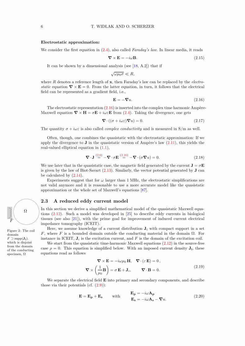
Here, we assume knowledge of a current distribution Ji with compact support in a setF , where F is a bounded domain outside the conducting material in the domain Ω. Forinstance in ICEIT, Ji is the excitation current, and F is the domain of the excitation coil.
We start from the quasistatic time-harmonic Maxwell equations (2.12) in the source-freecase ρ = 0. This equation is simplified below. With an imposed current density Ji, theseequations read as follows
∇ × E = −iωµ0 H, ∇ · (εE) = 0 ,
∇ ×(
1µ0
B
)
= σE + Ji, ∇ · B = 0.(2.19)
We separate the electrical field E into primary and secondary components, and describethose via their potentials (cf. (2.9)):
E = Ep + Es withEp = −iωAp
Es = −iωAs − ∇u.(2.20)
HYBRID TOMOGRAPHY FOR CONDUCTIVITY IMAGING 7
Here, Ap is the vector potential generated by the imposed current Ji (see (2.14)). Ap isassumed not to depend on the tissue conductivity. The secondary field As is the vectorpotential generated by σE.
For the representation of Ep we do not need a scalar potential, whereas for Es we do.Indeed, assume that Ep = −iωAp −∇up. Because the permittivity ε is constant in vacuum,we have ∇ · (εEp) = ε∇ · Ep = 0 (second equation in (2.19)). We use Coulomb’s gauge(2.10) for Ap, yielding
0 = ∇ · Ep = ∇ · (−iωAp − ∇up) = −iω∇ · Ap − ∇ · ∇up(2.10)
= −∆up. (2.21)
In the source-free case ρ = 0, the only solutions making physical sense are constant, andwithout loss of generality. we can take up ≡ 0 [37, 5.4,6.3]. In particular this means thatEp is completely determined by the vector potential Ap.
Now for biological tissue, it was observed in [25] that σE ≈ −σ(iωAp + ∇u). Thereforewe can work with
Enew := −iωAp − ∇u (2.22)
as an approximation for the electrical field. Using the third equation in (2.19), we have∇ · (∇×B) = ∇ · J = 0. Consequently, the following condition holds for the scalar potentialu:
∇ · (σ∇u) = −iωAp · ∇σ (2.23)
At the boundary ∂Ω of the conducting region we have σEnew · n = 0, as there is no currentflux through the boundary.
With Ap (calculated from the current Ji) and u, we find the electrical field Enew anda magnetic field Bnew (from (2.14)), which approximately satisfy (2.19). This has beenchecked in numerical simulations [25, A.C], [21] (see also [19]).
2.4 Acoustics
Equations for the acoustic pressure are obtained by linearization from the fundamentalequations of fluid dynamics, which relate the pressure p = p(x, t), the density ρ = ρ(x, t),and the velocity v = v(x, t) of the fluid, respectively.
Because it is a linearized model the variations of these parameters relative to a groundstate (p0(x), ρ0(x), 0) [54, §64] have to be small to be consistent with reality.
In particular, the standard wave equation
p :=1c2∂ttp− ∆p = 0, (2.24)
is derived from the linearized conservation principles for impulses, mass, and a relationbetween pressure and density, which read as follows:
ρ0∂tv + ∇p = 0 , (2.25)
∂tρ+ ρ0∇ · v = 0 , (2.26)
p = c2ρ. (2.27)
Here, c = c(x) =√
∂ρp(ρ0(x)) denotes the speed of sound in fluid dynamics (see [54, § 64]).Applying the divergence to (2.25) and calculating the time derivative of (2.26), we eliminatev to get ∆p = ∂ttρ. Substituting the time derivative of (2.27), we obtain the wave equation(2.24).
In the following, we assume that the fluid is perturbed by electromagnetic fields, causingthe Lorentz force (2.2) and Joule heating (2.3). We incorporate these effects into the equa-tions for the ultrasound pressure p. We first observe that the Lorentz force density f enters
8 T. WIDLAK AND O. SCHERZER
as a source term into the balance equation for the impulse (2.25), and we get
ρ0∂tv + ∇p− f = 0. (2.28)
Secondly, the linearized expansion equation, describes the relation between the energy ab-sorption, described by the power density function H , and the pressure
∂tp = ΓH + c2∂tρ . (2.29)
Here Γ is the dimensionless Grüneisen parameter. Very frequently it is assumed constant, butin fact is material dependent, and thus Γ = Γ(x). (2.29) can be derived from thermodynamicrelations and the principle of energy conservation [30, 0.1]. We emphasize that (2.29) is ageneralization of (2.27).
The wave equation with outer force and energy absorption is now derived from (2.28),(2.29) and the mass conservation principle (2.26). We arrive at the following inhomogeneouswave equation
p = −∇ · f(x, t) +Γc2∂tH(x, t) (2.30)
We will use this equation with f(x, t) = δ(t)φ(x) and H(x, t) = δ(t)ψ(x) in sections 4.2.1and 4.2.3.
Remark 1. By Duhamel’s principle (see [22, p. 81]), the solution of
p = δ(t)φ(x) + ∂tδ(t)ψ(x) , (2.31)
where δ is the δ-distribution, is the sum of the solutions of the inhomogeneous wave equations
P1(x, t) = 0P1(x, 0) = 0
∂t P1(x, 0) = φ(x) ,
P2(x, t) = 0P2(x, 0) = ψ(x)
∂t P2(x, 0) = 0 ,(2.32)
respectively.
3 MRI imaging
General comments and modeling of MRI
Magnetic Resonance Imaging (MRI) is frequently used as the basis for coupled Physicsimaging.
Since the modeling of MRI is not so common in Inverse Problems, it is reviewed here:MRI visualizes the nuclear magnetization M = M(x, t) resulting from selectively inducedmagnetic fields B = B(x, t). These two quantities are related by the simplified Bloch equa-tion:
∂tM = γM × B. (3.1)
Here γ denotes the gyromagnetic ratio specific to a proton. For instance, for hydrogen onehas γ = 4.6 · 107 T−1s−1.
For a stationary magnetic field in z-axis direction, B(x, t) = B(x) = (0, 0, B(x)), thesolution of the simplified Bloch equation with initial data M(x, 0) = M0(x) is given by [27,2.3.2]
M(x, t) =
Mx0 cos(−γB(x)t) −My
0 sin(−γB(x)t)Mx
0 sin(−γB(x)t) +My0 cos(−γB(x)t)
Mz0
.
This identity shows the rotation of the magnetization M around the z-axis when applyingthe stationary magnetic field (0, 0, B(x)). The quantity
ω(x) = −γB(x) (3.2)
HYBRID TOMOGRAPHY FOR CONDUCTIVITY IMAGING 9
B0
B1
BGz
BGy
BGx
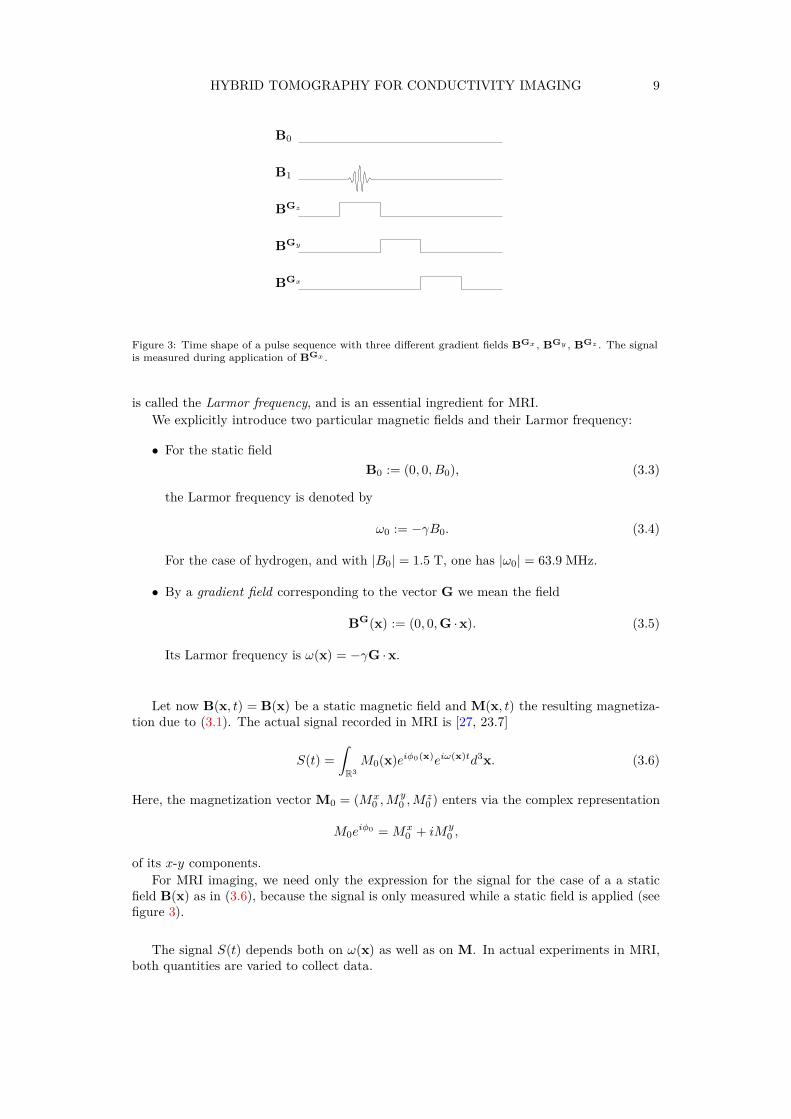
Figure 3: Time shape of a pulse sequence with three different gradient fields BGx , BGy , BGz . The signalis measured during application of BGx .
is called the Larmor frequency, and is an essential ingredient for MRI.We explicitly introduce two particular magnetic fields and their Larmor frequency:
• For the static field
B0 := (0, 0, B0), (3.3)
the Larmor frequency is denoted by
ω0 := −γB0. (3.4)
For the case of hydrogen, and with |B0| = 1.5 T, one has |ω0| = 63.9 MHz.
• By a gradient field corresponding to the vector G we mean the field
BG(x) := (0, 0,G · x). (3.5)
Its Larmor frequency is ω(x) = −γG · x.
Let now B(x, t) = B(x) be a static magnetic field and M(x, t) the resulting magnetiza-tion due to (3.1). The actual signal recorded in MRI is [27, 23.7]
S(t) =∫
R3
M0(x)eiφ0(x)eiω(x)td3x. (3.6)
Here, the magnetization vector M0 = (Mx0 ,M
y0 ,M
z0 ) enters via the complex representation
M0eiφ0 = Mx
0 + iMy0 ,
of its x-y components.For MRI imaging, we need only the expression for the signal for the case of a a static
field B(x) as in (3.6), because the signal is only measured while a static field is applied (seefigure 3).
The signal S(t) depends both on ω(x) as well as on M. In actual experiments in MRI,both quantities are varied to collect data.
10 T. WIDLAK AND O. SCHERZER
Experiment:
In magnetic resonance imaging experiments one applies different fields B in order to varyω(x) and M, such that sufficient data of S(t) can be collected to image the interior of thespecimen. In a general pulse sequence of MRI is a superposition of three magnetic fields,B0, B1, BG,
B(x, t) = B0(x) + B1(x, t) + BG(x, t) . (3.7)
B0 and BG are as in (3.4) and (3.5), respectively. Moreover, B1 = (B1(t) cos(ω1t), B1(t) sin(ω1t), 0)is a radio-frequency field. The time-shapes of the applied fields are depicted in figure 3.
The field B1 is responsible for creating a nontrivial M0. At every point where theresonance condition
ω1 = ω(x) (3.8)
holds, the magnetization vector is flipped away from the z-axis about a certain angle, andinconsequence, a non-zero transverse magnetization M0e
iφ0 results.Gradient fields with different vectors G are induced at different time (see figure 3).
Applying BGz with Gz = (0, 0, Gz) during the radio-frequency field, the resonance condition(3.8) is restricted to a small slice around the plane z = 0 (and only there M0 6= 0). Everysignal (3.6) recorded subsequently can be approximated by a 2D integrals (cf. [27, (10.34)]).
One applies BGy with Gy = (0, Gy, 0) in between the radio-frequency pulses and themeasurement for a certain time t′. At this time, the Larmor frequency changes to ω(x) =ω0 + Gyy. Afterwards, the phase of the transverse magnetization has changed from φ0 toφ0 + t′Gyy.
Now after making these preparations, measurements are taken and the signal (3.6) isrecorded. During the measurements, though, a gradient field BGz with Gx = (Gx, 0, 0) isapplied, which changes the Larmor frequency in (3.6) to ω(x) = ω0 + Gxx.
The upshot of applying these three types of gradient fields is that one can modify φ0 andω(x) in (3.6), such that one has access to the data
D(tGx, t′Gy) =
∫
R2
M0(x, y, 0)eiφ0eiγ(tGxx+t′Gyy)d(x, y). (3.9)
Introducing the 2D vector k = (tGx, t′Gy), (3.9) is just the 2D-Fourier transform with
respect to k of the transverse magnetization M0(x, y, 0)eiφ0 , sampled at the frequency vectork. By varying (Gx, Gy), and thus k, one collects data in the frequency regime from theFourier transform of M0(x, y, 0)eiφ0 ,
∫
R2
M0(x, y, 0)eiφ0eik · xd(x, y). (3.10)
The Fourier transform allows to recover M0(x, y, 0)eiφ0 .re
Remark 2. The modeling assumes that the magnetic fields in (3.7) have an ideal shape,and are not affected by the body tissue, in particular.
In fact, the radio-frequency field B1 is affected by electrical properties of the tissue. Thiseffect can be utilized to reconstruct the conductivity σ(x, ω0) using the Larmor frequencyω0 [40,41,101]. – This is one of several examples of imaging the electrical conductivity, orthe current density at the Larmor frequency, using the measurement setup of MRI (for otherapproaches see [73,93]).
4 Coupled Physics models for conductivity imaging
In this section we review coupled Physics techniques for imaging the scalar conductivity σfrom (2.6).
HYBRID TOMOGRAPHY FOR CONDUCTIVITY IMAGING 11
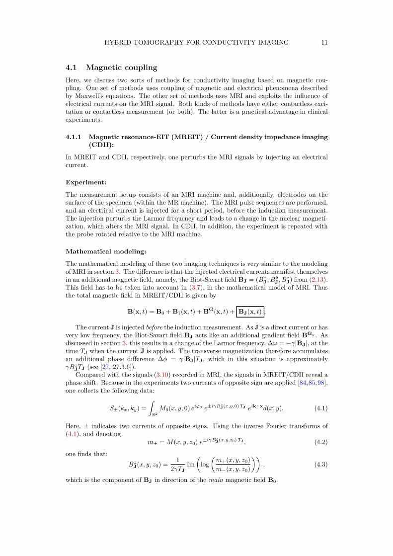
4.1 Magnetic coupling
Here, we discuss two sorts of methods for conductivity imaging based on magnetic cou-pling. One set of methods uses coupling of magnetic and electrical phenomena describedby Maxwell’s equations. The other set of methods uses MRI and exploits the influence ofelectrical currents on the MRI signal. Both kinds of methods have either contactless exci-tation or contactless measurement (or both). The latter is a practical advantage in clinicalexperiments.
4.1.1 Magnetic resonance-EIT (MREIT) / Current density impedance imaging(CDII):
In MREIT and CDII, respectively, one perturbs the MRI signals by injecting an electricalcurrent.
Experiment:
The measurement setup consists of an MRI machine and, additionally, electrodes on thesurface of the specimen (within the MR machine). The MRI pulse sequences are performed,and an electrical current is injected for a short period, before the induction measurement.The injection perturbs the Larmor frequency and leads to a change in the nuclear magneti-zation, which alters the MRI signal. In CDII, in addition, the experiment is repeated withthe probe rotated relative to the MRI machine.
Mathematical modeling:
The mathematical modeling of these two imaging techniques is very similar to the modelingof MRI in section 3. The difference is that the injected electrical currents manifest themselvesin an additional magnetic field, namely, the Biot-Savart field BJ = (Bx
J , ByJ, B
zJ) from (2.13).
This field has to be taken into account in (3.7), in the mathematical model of MRI. Thusthe total magnetic field in MREIT/CDII is given by
B(x, t) = B0 + B1(x, t) + BG(x, t) + BJ(x, t) .
The current J is injected before the induction measurement. As J is a direct current or hasvery low frequency, the Biot-Savart field BJ acts like an additional gradient field BGy . Asdiscussed in section 3, this results in a change of the Larmor frequency, ∆ω = −γ|BJ|, at thetime TJ when the current J is applied. The transverse magnetization therefore accumulatesan additional phase difference ∆φ = γ|BJ|TJ, which in this situation is approximatelyγBz
JTJ (see [27, 27.3.6]).Compared with the signals (3.10) recorded in MRI, the signals in MREIT/CDII reveal a
phase shift. Because in the experiments two currents of opposite sign are applied [84,85,98],one collects the following data:
S±(kx, ky) =∫
R2
M0(x, y, 0) eiϕ0 e±iγBzJ
(x,y,0) TJ eik · xd(x, y), (4.1)
Here, ± indicates two currents of opposite signs. Using the inverse Fourier transforms of(4.1), and denoting
m± = M(x, y, z0) e±iγBzJ
(x,y,z0) TJ , (4.2)
one finds that:
BzJ(x, y, z0) =
12γTJ
Im
(
log
(
m+(x, y, z0)m−(x, y, z0)
))
, (4.3)
which is the component of BJ in direction of the main magnetic field B0.
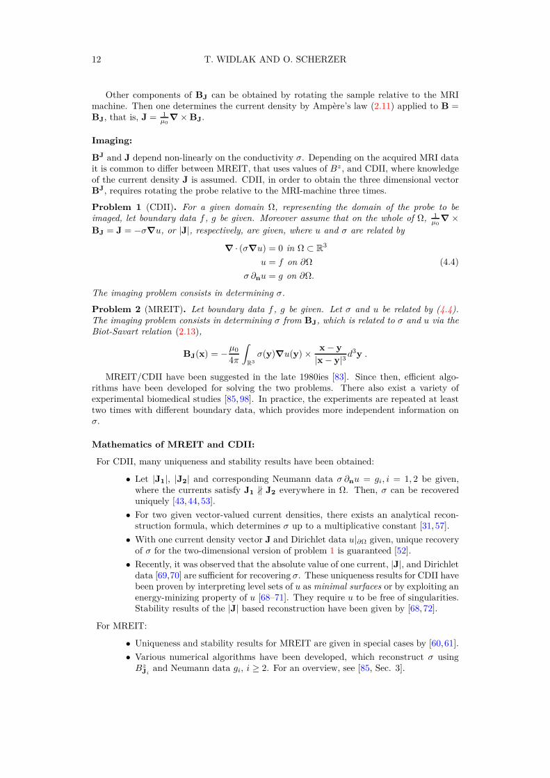
12 T. WIDLAK AND O. SCHERZER
Other components of BJ can be obtained by rotating the sample relative to the MRImachine. Then one determines the current density by Ampère’s law (2.11) applied to B =BJ, that is, J = 1
µ0
∇ × BJ.
Imaging:
BJ and J depend non-linearly on the conductivity σ. Depending on the acquired MRI datait is common to differ between MREIT, that uses values of Bz , and CDII, where knowledgeof the current density J is assumed. CDII, in order to obtain the three dimensional vectorBJ, requires rotating the probe relative to the MRI-machine three times.
Problem 1 (CDII). For a given domain Ω, representing the domain of the probe to beimaged, let boundary data f , g be given. Moreover assume that on the whole of Ω, 1
µ0
∇ ×BJ = J = −σ∇u, or |J|, respectively, are given, where u and σ are related by
∇ · (σ∇u) = 0 in Ω ⊂ R3
u = f on ∂Ω
σ ∂nu = g on ∂Ω.
(4.4)
The imaging problem consists in determining σ.
Problem 2 (MREIT). Let boundary data f , g be given. Let σ and u be related by (4.4).The imaging problem consists in determining σ from BJ, which is related to σ and u via theBiot-Savart relation (2.13),
BJ(x) = −µ0
4π
∫
R3
σ(y)∇u(y) × x − y
|x − y|3 d3y .
MREIT/CDII have been suggested in the late 1980ies [83]. Since then, efficient algo-rithms have been developed for solving the two problems. There also exist a variety ofexperimental biomedical studies [85, 98]. In practice, the experiments are repeated at leasttwo times with different boundary data, which provides more independent information onσ.
Mathematics of MREIT and CDII:
For CDII, many uniqueness and stability results have been obtained:
• Let |J1|, |J2| and corresponding Neumann data σ ∂nu = gi, i = 1, 2 be given,where the currents satisfy J1 ∦ J2 everywhere in Ω. Then, σ can be recovereduniquely [43, 44, 53].
• For two given vector-valued current densities, there exists an analytical recon-struction formula, which determines σ up to a multiplicative constant [31, 57].
• With one current density vector J and Dirichlet data u|∂Ω given, unique recoveryof σ for the two-dimensional version of problem 1 is guaranteed [52].
• Recently, it was observed that the absolute value of one current, |J|, and Dirichletdata [69,70] are sufficient for recovering σ. These uniqueness results for CDII havebeen proven by interpreting level sets of u as minimal surfaces or by exploiting anenergy-minizing property of u [68–71]. They require u to be free of singularities.Stability results of the |J| based reconstruction have been given by [68,72].
For MREIT:
• Uniqueness and stability results for MREIT are given in special cases by [60,61].
• Various numerical algorithms have been developed, which reconstruct σ usingBz
Jiand Neumann data gi, i ≥ 2. For an overview, see [85, Sec. 3].
HYBRID TOMOGRAPHY FOR CONDUCTIVITY IMAGING 13
4.1.2 Magnetic detection impedance tomography (MDEIT):
MDEIT uses magnetic boundary detection to recover currents and conductivity inside thetissue.
Experiment:
The equipment are electrodes to inject currents and several coils to record the magneticfield. A current is injected into the probe and the strength of the magnetic field is measuredby detector coils at different positions of the boundary. This technique is discussed in [36,45]and for practical applications see [62].
Mathematical modeling:
The mathematical model is the electrostatic model, ∇ · (σ∇u) = 0 from (2.18), which relatesthe electrical potential u and the conductivity σ. Neumann boundary conditions are given bythe injected currents. The Biot-Savart law (2.13) provides the relation between J = −σ∇uand the magnetic field B measured by the detector coils.
Imaging:
The imaging problem can be decomposed into two subproblems. In the first part, onereconstructs the current density J inside Ω from measurements of B at the boundary ∂Ω.In the second part, one faces exactly the same problem as in CDII, namely to reconstruct σfrom interior data of J (problem 2).
The inverse problem in the first step is a linear one: to recover J given the Biot-Savartlaw. We can restrict ourselves to current densities satisfying ∇ · J = 0, see (2.18).
Problem 3 (Inverse problem MDEIT, first step). Determine J|Ω from B|∂Ω using the Biot-Savart relation
B(x) =µ0
4π
∫
R3
J(y) × x − y
|x − y|3 d3y, x ∈ R3, (4.5)
taking into account that ∇ · J = 0.
The second problem is analogous to CDII (problem 2):
Problem 4 (Inverse problem MDEIT, second step). Let be given data f and g on ∂Ω.Determine σ from J = −σ∇u, which are related by (4.4).
Mathematical analysis:
The mathematical investigations relating to the linear problem 3 concern uniqueness is-sues and development of numerical algorithms. The kernel of the Biot-Savart operator, hasbeen investigated in [32, 45]. Uniqueness in the reconstruction problem has been shown forparticular cases, such as directed currents in layered media [32, 45, 78]. Different regular-ization methods have been applied to solve problem 3, and tested using real and simulateddata [33, 36].
4.1.3 EIT with induced currents (ICEIT)
ICEIT excites currents by magnetic induction and generates a voltage, which is measurableat the boundary of the probe.
14 T. WIDLAK AND O. SCHERZER
Experiment:
For the experiments, one uses coils and electrodes. A time harmonic current is produced inthe excitation coil and eddy currents are induced in the tissue. The voltages are detectedat the boundary of the probe [25, 102].
Modeling:
We recall the setting of the reduced eddy current model in section 2.3, referring to figure2. The excitation coil lies in a domain F where the excitation current Ji is supported. Theconducting tissue is in the domain Ω, disjoint from F .
In (2.22), we have introduced a reduced version of the electrical field as
E = −iωAp − ∇u,
where Ap is the primary vector potential generated by the excitation current Ji (see (2.14)).The scalar potential is governed by (2.23) with boundary condition E · n = 0 on ∂Ω. Toensure a unique solution, we require that
∫
∂ΩudS = 0. This gives the description of the
eddy currents inside the tissue.The measurement data consist of (finitely many) line integrals
∫ x2
x1
E · dl. Because thedeterminatino of Ap via (2.14) does not depend on inhomogeneities of σ, one obtains lineintegrals of ∇u, which are potential differences. As in classical EIT, these correspondapproximately to knowledge of Dirichlet data u|∂Ω, if one chooses a voltage reference. Forthis, we assume
∫
∂Ω u dS = 0.
Imaging:
The imaging problem in ICEIT is an inverse boundary value problem:
Problem 5 (Inverse problem ICEIT). Let (σ, u) satisfy
∇ · (σ∇u) = −iωAp · ∇σ in Ω
∂nu = −iωAp · n on ∂Ω∫
∂Ω
u dS = 0.
(4.6)
Given are boundary data u|∂Ω and the primary potential Ap|Ω in Ω, which is related to theexcitation current Ji on R2 by
Ap(x) =µ0
4π
∫
R2
Ji(y)|x − y|d
3y. (4.7)
Determine σ.
Mathematics and Numerics:
ICEIT has been investigated numerically: Different regularization procedures have beenapplied, e.g., in [25, 102].
4.1.4 Magnetic induction tomography (MIT):
In MIT, eddy currents are induced, and the resulting magnetic fields are measured at theboundary.
HYBRID TOMOGRAPHY FOR CONDUCTIVITY IMAGING 15
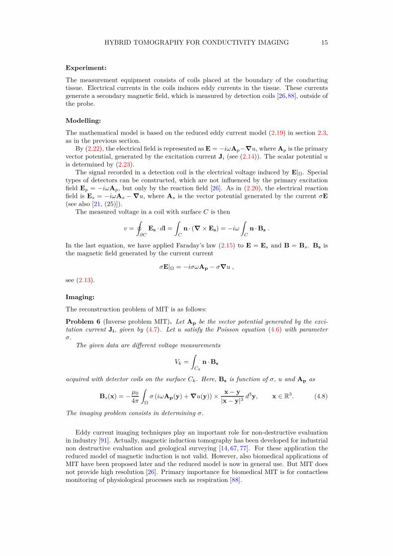
Experiment:
The measurement equipment consists of coils placed at the boundary of the conductingtissue. Electrical currents in the coils induces eddy currents in the tissue. These currentsgenerate a secondary magnetic field, which is measured by detection coils [26,88], outside ofthe probe.
Modelling:
The mathematical model is based on the reduced eddy current model (2.19) in section 2.3,as in the previous section.
By (2.22), the electrical field is represented as E = −iωAp−∇u, where Ap is the primaryvector potential, generated by the excitation current Ji (see (2.14)). The scalar potential uis determined by (2.23).
The signal recorded in a detection coil is the electrical voltage induced by E|Ω. Specialtypes of detectors can be constructed, which are not influenced by the primary excitationfield Ep = −iωAp, but only by the reaction field [26]. As in (2.20), the electrical reactionfield is Es = −iωAs − ∇u, where As is the vector potential generated by the current σE(see also [21, (25)]).
The measured voltage in a coil with surface C is then
v =∮
∂C
Es · dl =∫
C
n · (∇ × Es) = −iω∫
C
n · Bs .
In the last equation, we have applied Faraday’s law (2.15) to E = Es and B = Bs. Bs isthe magnetic field generated by the current current
σE|Ω = −iσωAp − σ∇u ,
see (2.13).
Imaging:
The reconstruction problem of MIT is as follows:
Problem 6 (Inverse problem MIT). Let Ap be the vector potential generated by the exci-tation current Ji, given by (4.7). Let u satisfy the Poisson equation (4.6) with parameterσ.
The given data are different voltage measurements
Vk =∫
Ck
n · Bs
acquired with detector coils on the surface Ck. Here, Bs is function of σ, u and Ap as
Bs(x) = −µ0
4π
∫
Ω
σ (iωAp(y) + ∇u(y)) × x − y
|x − y|3 d3y, x ∈ R3. (4.8)
The imaging problem consists in determining σ.
Eddy current imaging techniques play an important role for non-destructive evaluationin industry [91]. Actually, magnetic induction tomography has been developed for industrialnon destructive evaluation and geological surveying [14, 67, 77]. For these application thereduced model of magnetic induction is not valid. However, also biomedical applications ofMIT have been proposed later and the reduced model is now in general use. But MIT doesnot provide high resolution [26]. Primary importance for biomedical MIT is for contactlessmonitoring of physiological processes such as respiration [88].
16 T. WIDLAK AND O. SCHERZER
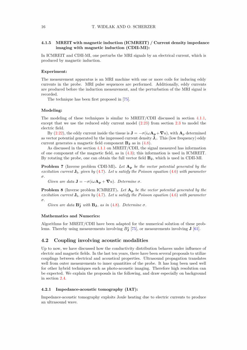
4.1.5 MREIT with magnetic induction (ICMREIT) / Current density impedanceimaging with magnetic induction (CDII-MI):
In ICMREIT and CDII-MI, one perturbs the MRI signals by an electrical current, which isproduced by magnetic induction.
Experiment:
The measurement apparatus is an MRI machine with one or more coils for inducing eddycurrents in the probe. MRI pulse sequences are performed. Additionally, eddy currentsare produced before the induction measurement, and the perturbation of the MRI signal isrecorded.
The technique has been first proposed in [75].
Modeling:
The modeling of these techniques is similar to MREIT/CDII discussed in section 4.1.1,except that we use the reduced eddy current model (2.23) from section 2.3 to model theelectric field.
By (2.22), the eddy current inside the tissue is J = −σ(iωAp +∇u), with Ap determinedas vector potential generated by the impressed current density Ji. This (low frequency) eddycurrent generates a magnetic field component BJ as in (4.8).
As discussed in the section 4.1.1 on MREIT/CDII, the signal measured has informationof one component of the magnetic field, as in (4.3); this information is used in ICMREIT.By rotating the probe, one can obtain the full vector field BJ, which is used in CDII-MI.
Problem 7 (Inverse problem CDII-MI). Let Ap be the vector potential generated by theexcitation current Ji, given by (4.7). Let u satisfy the Poisson equation (4.6) with parameterσ.
Given are data J = −σ(iωAp + ∇u). Determine σ.
Problem 8 (Inverse problem ICMREIT). Let Ap be the vector potential generated by theexcitation current Ji, given by (4.7). Let u satisfy the Poisson equation (4.6) with parameterσ.
Given are data BzJ with BJ, as in (4.8). Determine σ.
Mathematics and Numerics:
Algorithms for MREIT/CDII have been adapted for the numerical solution of these prob-lems. Thereby using measurements involving Bz
J [75], or measurements involving J [61].
4.2 Coupling involving acoustic modalities
Up to now, we have discussed how the conductivity distribution behaves under influence ofelectric and magnetic fields. In the last ten years, there have been several proposals to utilizecouplings between electrical and acoustical properties. Ultrasound propagation translateswell from outer measurements to inner quantities of the probe. It has long been used wellfor other hybrid techniques such as photo-acoustic imaging. Therefore high resolution canbe expected. We explain the proposals in the following, and draw especially on backgroundin section 2.4.
4.2.1 Impedance-acoustic tomography (IAT):
Impedance-acoustic tomography exploits Joule heating due to electric currents to producean ultrasound wave.
HYBRID TOMOGRAPHY FOR CONDUCTIVITY IMAGING 17
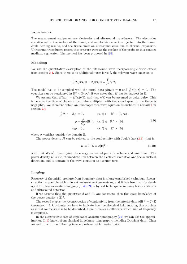
Experiments:
The measurement equipment are electrodes and ultrasound transducers. The electrodesare attached to the surface of the tissue, and an electric current is injected into the tissue.Joule heating results, and the tissue emits an ultrasound wave due to thermal expansion.Ultrasound transducers record this pressure wave at the surface of the probe or in a contactmedium, e.g. water. The method has been proposed in [24].
Modeling:
We use the quantitative description of the ultrasound wave incorporating electric effectsfrom section 2.4. Since there is no additional outer force f , the relevant wave equation is
1c2∂ttp(x, t) − ∆p(x, t) =
Γc2∂tH,
The model has to be supplied with the initial data p(x, t) = 0 and ∂∂tp(x, t) = 0. The
equation can be considered in Rn × (0,∞), if one notes that H has its support in Ω.We assume that H(x, t) = H(x)g(t), and that g(t) can be assumed as delta pulse. This
is because the time of the electrical pulse multiplied with the sound speed in the tissue isnegligible. We therefore obtain an inhomogeneous wave equation as outlined in remark 1 insection 2.4:
1c2∂ttp− ∆p = 0 , (x, t) ∈ Rn × (0,∞) ,
p =β
Cp
σ|E|2 , (x, t) ∈ R⋉ × 0 ,
∂tp = 0 , (x, t) ∈ Rn × 0 ,
(4.9)
where σ vanishes outside the domain Ω.The power density H can be related to the conductivity with Joule’s law (2.3), that is,
H = J · E = σ|E|2, (4.10)
with unit W/m3, quantifying the energy converted per unit volume and unit time. Thepower density H is the intermediate link between the electrical excitation and the acousticaldetection, and it appears in the wave equation as a source term.
Imaging:
Recovery of the initial pressure from boundary data is a long-established technique. Recon-struction is possible with different measurement geometries, and it has been mainly devel-oped for photo-acoustic tomography, [49,59], a hybrid technique combining laser excitationand ultrasound detection.
If we assume that the quantities β and Cp are constants, then this gives knowledge ofthe power density σ|E|2.
The second step is the reconstruction of conductivity from the interior data σ|E|2 = J · Ethroughout Ω. Obviously, we have to indicate how the electrical field entering this problemas initial source state is to be described. Here it makes a difference which kind of frequencyis employed.
In the electrostatic case of impedance-acoustic tomography [24], we can use the approx-imation (1.1) known from classical impedance tomography, including Dirichlet data. Thenwe end up with the following inverse problem with interior data:
18 T. WIDLAK AND O. SCHERZER
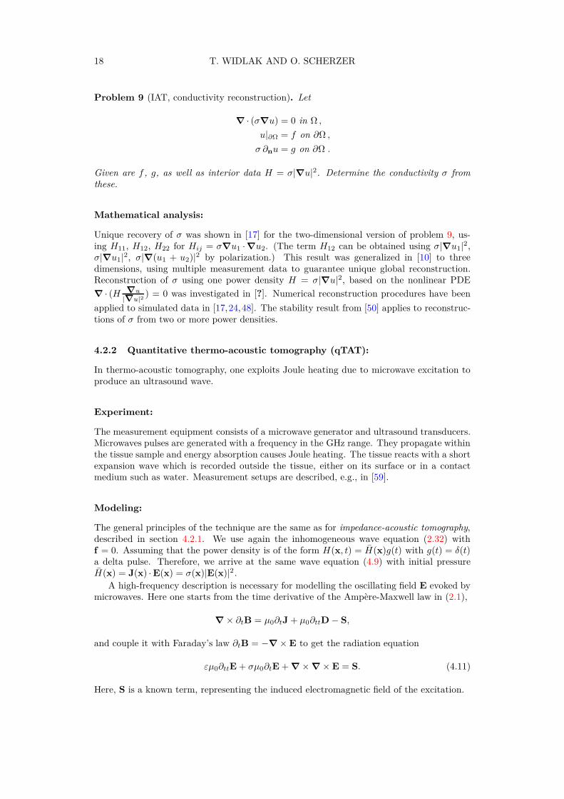
Problem 9 (IAT, conductivity reconstruction). Let
∇ · (σ∇u) = 0 in Ω ,
u|∂Ω = f on ∂Ω ,
σ ∂nu = g on ∂Ω .
Given are f , g, as well as interior data H = σ|∇u|2. Determine the conductivity σ fromthese.
Mathematical analysis:
Unique recovery of σ was shown in [17] for the two-dimensional version of problem 9, us-ing H11, H12, H22 for Hij = σ∇u1 · ∇u2. (The term H12 can be obtained using σ|∇u1|2,σ|∇u1|2, σ|∇(u1 + u2)|2 by polarization.) This result was generalized in [10] to threedimensions, using multiple measurement data to guarantee unique global reconstruction.Reconstruction of σ using one power density H = σ|∇u|2, based on the nonlinear PDE
∇ · (H ∇u
|∇u|2) = 0 was investigated in [?]. Numerical reconstruction procedures have been
applied to simulated data in [17,24,48]. The stability result from [50] applies to reconstruc-tions of σ from two or more power densities.
4.2.2 Quantitative thermo-acoustic tomography (qTAT):
In thermo-acoustic tomography, one exploits Joule heating due to microwave excitation toproduce an ultrasound wave.
Experiment:
The measurement equipment consists of a microwave generator and ultrasound transducers.Microwaves pulses are generated with a frequency in the GHz range. They propagate withinthe tissue sample and energy absorption causes Joule heating. The tissue reacts with a shortexpansion wave which is recorded outside the tissue, either on its surface or in a contactmedium such as water. Measurement setups are described, e.g., in [59].
Modeling:
The general principles of the technique are the same as for impedance-acoustic tomography,described in section 4.2.1. We use again the inhomogeneous wave equation (2.32) withf = 0. Assuming that the power density is of the form H(x, t) = H(x)g(t) with g(t) = δ(t)a delta pulse. Therefore, we arrive at the same wave equation (4.9) with initial pressureH(x) = J(x) · E(x) = σ(x)|E(x)|2 .
A high-frequency description is necessary for modelling the oscillating field E evoked bymicrowaves. Here one starts from the time derivative of the Ampère-Maxwell law in (2.1),
∇ × ∂tB = µ0∂tJ + µ0∂ttD − S,
and couple it with Faraday’s law ∂tB = −∇ × E to get the radiation equation
εµ0∂ttE + σµ0∂tE + ∇ × ∇ × E = S. (4.11)
Here, S is a known term, representing the induced electromagnetic field of the excitation.

HYBRID TOMOGRAPHY FOR CONDUCTIVITY IMAGING 19
Imaging:
The initial pressure distribution can be obtained by acoustic reconstruction formulas. Tocalculate the conductivity σ, we have now the quantitative aspect of thermo-acoustic to-mography:
Problem 10 (qTAT). Let
εµ0∂ttE + σµ0∂tE + ∇ × ∇ × E = S
with known S and constant ε, µ0.Determine the conductivity σ from knowledge of S and σ|E|2.
In [11], unique recovery of σ from H = σ(x)|E(x)|2 is shown for a class of boundedconductivity distributions (assuming that ε ≡ const.).
4.2.3 Magneto-acoustic tomography with magnetic induction (MAT-MI):
Magneto-acoustic tomography exploits the Lorentz force effect to create a pressure wave.
Experiment:
The measurement equipment consists of an excitation coil, a static magnet and ultrasoundtransducers. While the tissue is kept in the static magnetic field, electrical pulses in theexcitation coil induce a eddy currents in the tissue. These, in turn, are affected by theLorentz force due to the static field. The force causes the tissue to displace locally, and apressure wave results. This wave reaches the boundary, where ultrasound transducers recordthe signal, either at the surface of the body or in a contact medium, such as water.
Experimental setups with different arrangements of induction coils are documented in[34, 99].
Mathematical modeling:
We model the ultrasound wave motion with the wave equation with outer force f . Applying(2.2) with vanishing charge density ρ = 0 to the static field B = B0, we obtain the expressionfor the Lorentz force density f = J × B0 (see also [79]). Following the discussion in section2.4, the quantitative description of the acoustic wave is governed by
1c2∂ttp(x, t) − ∆p(x, t) = −∇ · (J × B0) +
Γc2∂tH,
where H quantifies the absorbed energy due to eddy currents. Notwithstanding, the energyabsorption effect can be ignored in the experiments of [99]. There, magnetic induction isused for excitation of electrical currents, and this entails smaller field strengths. Consideringthe usual scale of conductivity in biological tissue, the pressure due to the thermo-acousticeffect can be neglected compared with pressure due to Lorentz force2 (see also [99, p. 5179]).
Therefore the model is
1c2∂ttp(x, t) − ∆p(x, t) = −∇ · (J × B0), (4.12)
together with the initial and boundary conditions
p(0) = 0, ∂tp(0) = 0. (4.13)
We assume that the time- and space variables can be separated. The inhomogeneity fis therefore ∇ · f (x)g(t), where f is the force density −J × B0 = −σ(x)E(x) × B0(x). Due
2 Y. Xu, personal communication

20 T. WIDLAK AND O. SCHERZER
to the different frequency ranges of the electrical and the acoustical pulse, we assume againthat g is a delta distribution. According to Duhamel’s principle (2.32), the inhomogeneousproblem (4.12) and (4.13) can be converted to a Cauchy problem for the homogeneous waveequation [5, 6]:
1c2∂ttp− ∆p = 0 (x, t) ∈ Ω × (0,∞)
p = 0 x ∈ ∂Ω
∂tp = −∇ · (σE × B0) t = 0
p = 0 t = 0.
(4.14)
Imaging:
The first step of the reconstruction of the source term ∇ · (σE × B0). In contrast to thetechniques of impedance-acoustic tomography and thermo-acoustic tomography, we nowlook for the initial velocity of the pressure, which can be recovered as well.
As quantitative problem, it remains to recover the distribution of the conductivity σ overΩ. For this purpose, one has to describe the electrical field E. For this, we use the eddycurrent model (2.23) discussed in section 2.3, adapted here for the pulsed excitation current.Therefore, the hybrid imaging problem is
Problem 11 (Inverse problem MAT-MI). Let
∇ · (σ∇u) = −∂tAp · ∇σ in Ω
∂nu = −∂tAp · n on ∂Ω∫
∂Ω
u dS = 0.
The vector potential Ap|Ω on R3 is determined from the excitation current current Ji|F by
Ap(x, t) =µ0
4π
∫
R2
Ji(y, t)|x − y| d
3y.
Given are B0 and ∇ · (σ(∂tAp + ∇u) × B0), from which to determine σ.
4.2.4 Magneto-acoustic-electrical tomography (MAET):
In MAET, pressure waves excite the tissue, and a voltage is produced due to the Lorentzforce effect.
Experiment:
The measurement equipment in MAET consists of a permanent magnet, a waveform gener-ator, and of electrodes to measure the voltage at the boundary. The sample is put into thestatic magnetic field, and expopsed to different ultrasound waves. Due to frictional forces,the ions in the tissue move. As there is a magnetic field present, the electrical charges sepa-rate by the Lorentz force mechanism. A voltage results, which is detected on the surface ofthe probe. – The experiment is repeated with different arrangements of the static field.
The physical effect underlying this technique has been studied in [66,94], further imagingexperiments have been reported in [29].

HYBRID TOMOGRAPHY FOR CONDUCTIVITY IMAGING 21
Modeling:
To model MAET, we follow the approach in [51]. We assume that the static magnetic field Bin the experiments is homogeneous, that is, B(x) = B. The Lorentz force exerted upon themoving particles gives rise to an impressed current density JL which is approximately [51,66]
JL(x, t) = σ(x)B × v(x, t),
where v is the velocity field of the fluid.For each time t the electrical field inside the domain Ω is described by an electrical
potential, E(x, t) = −∇u(x, t). In absence of any other free charges, the potentials can bedescribed by the conditions ∇ · J = 0 and J · n = 0 for the total current J = −σ∇u + JL,that is
∇ · (σ∇u) = −∇ · (σB × v), x in Ω
∂nu = −(B × v) · n, x on ∂Ω(4.15)
The voltage measured at the boundary gives knowledge of u(x, t)|∂Ω. One can alsoassume that only a weighted average of u is known, that is
M(t) =∫
∂Ω
I(x)u(x, t)dS(x). (4.16)
Mathematical analysis:
Using identities from vector analysis, it can be shown that the measurements in (4.16) are
M(t) = −B ·∫
Ω
JI × v d3x , (4.17)
with the current density JI(x) = −σ∇uI(x) satisfying the electrostatic equation
∇ · (σ∇uI) = 0, x in Ω
σ∂nuI = I(x), x on ∂Ω.(4.18)
The inverse problem is
Problem 12 (MAET). Let uI satisfy (4.18). Determine σ from knowledge of M(t) in(4.17), by possibly varying B, I, and v.
Reconstructions for the case of general acoustic waves have been given in [51]. Theprocedure leads to knowledge of several vector valued current densities JI , which in the laststep are converted to σ. This is a problem of current density impedance imaging (CDII),discussed in section 4.1.1. Reconstructions for the case of focused ultrasound excitation aregiven in [5].
4.2.5 Acousto-electrical tomography (AET):
An EIT experiment is performed and, in addition, the conductivity values are perturbed viaultrasound excitation in parallel.
Experiment:
For the measurements, one needs the typical EIT electrode setup and a device to produceultrasound waves to excite the probe. The standard EIT measurement protocol is performed.For the perturbation of the conductivity, a set of various ultrasound waves is applied. Theboundary voltages due to the perturbation are then compared with the standard voltages.
The method was proposed in [100]. The underlying physical effect is treated in [56].
22 T. WIDLAK AND O. SCHERZER
Modeling:
The standard electrostatic equation from (2.18) is used to model the electrical potential u,
∇ · (σ∇u) = 0 in Ω
σ ∂nu = g on ∂Ω.
We now assume that the probe is excited by focused ultrasound beams. Therefore, theconductivity (which depends on the pressure), is perturbed in a domain D = z + δB, whereB is the unit disc and z is the center of focus. The perturbed conductivity is denoted σδ
z;the new potential uδ is therefore described by
∇ · (σδz∇uδ
z) = 0 in Ω
σδz ∂nu
δz = g on ∂Ω.
As measurement data, we have the difference of the measured voltages at the boundary, i.e.uδ − u|∂Ω.
Mathematical analysis:
It is shown in [4], that for δ → 0, one has the asymptotic formula
∫
∂Ω
(uδ − u) g dS = |∇u(z)|2∫
D
σ(y)(η(y) − 1)2
η(y) + 1d3y + o(vol(D)).
Here, η is a known function in Ω.From this formulation, one notices that the measurement data give knowledge of the
power density at z, σ(z)|∇u(z)|2, up to a small error.
Imaging:
The inverse problem is to recover the conductivity σ from the interior information σ|∇u|.This problem is identical with problem 9 of impedance-acoustic tomography.
Problem 13 (AET, conductivity determination). Let
∇ · (σ∇u) = 0 in Ω
u|∂Ω = f on ∂Ω
σ ∂nu = g on ∂Ω.
Given are f , g, as well as interior data H = σ|∇u|2. Determine σ.
Mathematical analysis:
In the modeling of AET, we have assumed that σδz −σ are approximately delta-distributions.
But this restriction can be overcome and other more practical forms of ultrasound pertur-bation (such as plane waves, e.g.) can be used [47], [48, Section 2].
For this we consider
Lσ(f)(y) =∫
Ω
k(x,y)f(x) d3x
where Lσ maps an increment f = dσ of conductivity to the corresponding perturbationLσf in the boundary voltage. As perfect focusing of ultrasound waves correspond to δ-distributions f , and this would correspond to simple evaluation of the kernel k(x, y). Itis more realistic that ultrasound waves of other, unfocused type, trigger the corresponding

HYBRID TOMOGRAPHY FOR CONDUCTIVITY IMAGING 23
Table 3: Electromagnetic variants of the Calderón problem in different frequency ranges.
Technique equation in Ω boundary data remarks
EITeqn. (1.1)
∇ ·σ∇u = 0uσ ∂nu
IC-EITsection 4.1.3
∇ · (σ∇u) = −iωA · ∇σuσ ∂nu = −iωA · n
excitation A known
MITsection 4.1.4
∇ · (σ∇u) = −iωA · ∇σ
∫
Cn · B
σ ∂nu = −iωA · n excitation A known.B = B(σ, u,A),C is a coil surfaceoutside Ω.
MD-EITsection 4.1.2
B =∫
J×R|R|3 B recover J, not σ
conductivity changes, proportional to the pressure. So, the intermediate step (syntheticfocusing) corresponds to finding the values of the kernel k(x, y) by measurements of
∫
Ω
k(x,y)wα(x)d3x
for a particular class of waves wα. Synthetic focusing for spherical waves, plane waves hasbeen discussed in [47, Section 2]; numerical calculations are performed in [48].
5 Summary
The hybrid imaging techniques and mathematical models discussed above are summarizedin the following tables 4, 5. Those, consist of four columns, summarizing the imaging data,the overspecified data of the quantitative inverse problem, and the equations of the forwardproblems. In mathematical terms, in general, these are inverse problems with interior data.The table, however, does not summarize unique identifability and unique reconstructabilityof the quantitative imaging data. Hybrid models coupling magnetic resonance effects withcurrent densities are listed in table 4. Some of these, like MREIT/CDII, rely on the low-frequency description ∇ · (σ∇u) = 0, others use radiofrequency currents, where neitherelectrostatic nor quasistatic approximations are applicable. Coupling hybrid techniqueswith ultrasound modalities are summarized in table 5. They also range from low-frequencyor quasistatic to high-frequency ranges.
In addition to coupled Physics (hybrid) techniques with interior information, we alsosummarize the standard EIT problem (the Calderón problem) together with techniquesusing electromagnetic coupling in several frequency ranges (see tables 3). The correspondingreconstruction cannot be separated into two imaging problems with interior data.
Shortly, we also mention some hybrid imaging techniques using other physical parame-ters, which nevertheless are formally related to the models using the electrostatic regime,∇ · (σ∇u) = 0:
In quantitative photoacoustic tomography (qPAT) in the diffusion regime, the diffusivityκ is reconstructed, while the absorption µ in the elliptic equation ∇ · (κ∇u) + µu = 0is known. The imaging data are H = µI [11].
In microwave tomography, the generalization of AET, one recovers the parameters a and qin ∇ · (a∇u) + k2 q u = 0, with a|∇u|2 and q|u| given [6].

24 T. WIDLAK AND O. SCHERZER
Table 4: Coupled Physics models with interioir data, based on MRI.
Technique interior data equation in Ω boundary data remarksCDII
section 4.1.1σ∇u orσ|∇u| ∇ · (σ∇u) = 0 u
MREITsection 4.1.1
Bz∇ · (σ∇u) = 0 σ ∂nu Bz = F (σ∇u, σ)
CDII-MIsection 4.1.5
σE ∇ · (σ∇u) = −iωA · ∇σ σ ∂nu = iωA · n excitation AknownE = −iωA − ∇u
ICMREITsection 4.1.5
Bz∇ · (σ∇u) = −iωA · ∇σ σ ∂nu = iωA · n excitation A
knownBz = F (σ∇u, σ)
Table 5: Coupled Physics models with interior data, based on Ultrasound.
Technique interior data equation in Ω boundary data remarks
IATsection 4.2.1
σ|∇u|2 ∇ · (σ∇u) = 0 uσ∂nu
qTATsection 4.2.2
σ|∇u|2 εµ0∂ttE + σµ0∂tE+∇ × ∇ × E = S
S|F F ∩ Ω = ∅
MAT-MIsection 4.2.3
∇ · (σE × B0) ∇ · (σ∇u) = −∂tA · ∇σ σ ∂nu = −∂tA · n excitation Aknown,E = −∂tA − ∇u
MAETsection 4.2.4
B ·∫
σ∇uI ×v ∇ · (σ∇uI) = 0 uI
σ∂nuI = IB ·
∫
Ωσ∇uI ×
v =∫
∂Ω I u dSAET
section 4.2.5σ|∇u|2 ∇ · (σ∇u) = 0 u
σ∂nu
HYBRID TOMOGRAPHY FOR CONDUCTIVITY IMAGING 25
In Optoacoustic tomography one also recovers σ in ∇ · (σ∇u) = 0 with σ|∇u|2 given, hereσ is the optical absorption [12].
6 Acknowledgements
We thank Barbara Kaltenbacher for helpful discussions and Yuan Xu, Eung Je Woo, DogaGürsoy and Hermann Scharfetter for information concerning the special techniques. Thiswork has been supported by the Austrian Science Fund (FWF) within the national researchnetwork Photoacoustic Imaging in Biology and Medicine, project S10505-N20.
References
[1] A. Adler, R. Gaburro, and W. Lionheart. Electrical impedance tomography. In Ot-mar Scherzer, editor, Handbook of Mathematical Methods in Imaging, pages 599–652.Springer, 2011.
[2] A. P. Aizebeokhai. 2D and 3D geoelectrical resistivity imaging: theory and field design.Sci. Res. Essays, 23:3592–3605, 2010.
[3] G. Alessandrini. Stable determination of conductivity by boundary measurements.Appl. Anal., 27:153–172, 1988.
[4] H. Ammari, E. Bonnetier, Y. Capdeboscq, M. Tanter, and M. Fink. Electricalimpedance tomography by elastic deformation. SIAM J. Appl. Math., 68(6):1557–1573, 2008.
[5] H. Ammari, Y. Capdeboscq, H. Kang, and A. Kozhemyak. Mathematical modelsand reconstruction methods in magneto-acoustic imaging. European J. Appl. Math.,20(3):303–317, 2009.
[6] H. Ammari and H. Kang. Expansion methods. In O. Scherzer, editor, [81], pages447–500. Springer, 2011.
[7] G. B. Arfken and H. J. Weber. Mathematical Methods for Physicists. Academic Press,5 edition, 2001.
[8] K. Astala and L. Päivärinta. Calderón’s inverse conductivity problem in the plane.Ann. Math., 163:265–99, 2006.
[9] G. Bal. Hybrid inverse problems and internal information. preprint, 2011.http://arxiv.org/abs/1110.4733v1.
[10] G. Bal, E. Bonnetier, F. Monard, and F. Triki. Inverse diffusion from knowledge ofpower densities. preprint, 2011. http://arxiv.org/abs/1110.4577v1.
[11] G. Bal, K. Ren, G. Uhlmann, and T. Zhou. Quantitative thermo-acoustics and relatedproblems. Inverse Probl., 27:055007, 2010.
[12] G. Bal and J. C. Schotland. Inverse scattering and acousto-optic imaging. Phys. Rev.Lett., 104:043902, 2010.
[13] R. H. Bayford. Bioimpedance tomography (electrical impedance tomography). Annu.Rev. Biomed. Eng., 8:63–91, 2006.
[14] R. Binns, A. R. A. Lyons, A. J. Peyton, and W. D. N. Pritchard. Imaging moltensteel flow profiles. Meas. Sci. Technol., 12:1132–1138, 2001.
26 T. WIDLAK AND O. SCHERZER
[15] L. Borcea. Electrical impedance tomography. Inverse Probl., 18:R99–R136, 2002.
[16] A. P. Calderón. On an inverse boundary value problem. In Seminar on numericalanalysis and its applications to continuum physics, pages 65–73. Soc. Brasil. Mat., Riode Janeiro, 1980.
[17] Y. Capdeboscq, J. Fehrenbach, F. de Gournay, and O. Kavian. Imaging by modi-fication: numerical reconstruction of local conductivities from corresponding powerdensity measurements. SIAM J. Imaging Sciences, 2(4):1003–1030, 2009.
[18] M. Cheney, D. Isaacson, and J. C. Newell. Electrical impedance tomography. SIAMRev., 41(1):85–101, 1999.
[19] B. Dekdouk, W. Yin, Ch. Ktistis, D. W. Armitage, and A. J. Peyton. A method tosolve the forward problem in magnetic induction tomography based on the weaklycoupled field approximation. IEEE Trans. Biomed. Eng., 57(4):914–921, 2010.
[20] C. Emiliani. Planet Earth. Cosmology, Geology, and the Evolution of Life and Envi-ronment. Cambridge University Press, 1992.
[21] S. Engleder and O. Steinbach. Boundary integral formulations for the forward problemin magnetic induction tomography. Math. Methods Appl. Sci., pages 1144–1156, 2011.
[22] L. C. Evans. Partial Differential Equations, volume 19 of Graduate Studies in Math-ematics. American Mathematical Society, Providence, RI, 1998.
[23] S. Gabriel, R. W. Lau, and C. Gabriel. The dielectric properties of biological tissues:Ii. measurements in the frequency range 10 hz to 20 ghz. Phys. Med. Biol., 41:2251–69,1996.
[24] B. Gebauer and O. Scherzer. Impedance-acoustic tomography. SIAM J. Appl. Math.,69(2):565–576, 2008.
[25] N. G. Gençer, M. Kozuoglu, and Y. Z. İder. Electrical impedance tomography usinginduced currents. IEEE Trans. Med. Imag., 13(2):338–350, 1994.
[26] D. Gürsoy and H. Scharfetter. Optimum receiver array design for magnetic inductiontomography. IEEE Trans. Biomed. Eng., 56(5):1435–41, 2009.
[27] E. M. Haacke, R. W. Brown, M. R. Thompson, and R. Venkatesan. Magnetic Reso-nance Imaging: Physical Principles and Sequence Design. Wiley, New York, 1999.
[28] D. Haemmerich, S. T. Stalin, J. Z. Tsai, S. Tungjitkusolmun, D. M. Mahvi, and J. G.Webster. In vivo electrical conductivitiy of hepatic tumours. Physiol. Meas., 24:251–260, 2003.
[29] S. Haider, A. Hrbek, and Y. Xu. Magneto-acousto-electrical tomography: a potentialmethod for imaging current density and electrical impedance. Physiol. Meas., 29:S41–S50, 2008.
[30] M. Haltmeier. Frequency domain reconstruction for photo- and thermoacoustic to-mography with line detectors. Math. Models Methods Appl. Sci., 19(2):283–306, 2009.
[31] K. F. Hasanov, A. W. Ma, A. I. Nachman, and M. L. G. Joy. Current densityimpedance imaging. IEEE Trans. Med. Imag., 27(9):1301–1309, 2008.
[32] K.-H. Hauer, L. Kühn, and R. Potthast. On uniqueness and non-uniqueness for currentreconstruction from magnetic fields. Inverse Probl., 21(3):955–967, 2005.

HYBRID TOMOGRAPHY FOR CONDUCTIVITY IMAGING 27
[33] K.-H. Hauer, R. Potthast, and M. Wannert. Algorithms for magnetic tomography –on the role of a priori knowledge and constraints. Inverse Probl., 24(4):045008, 2008.
[34] G. Hu, X. Li, and B. He. Imaging biological tissues with electrical conductivity contrastbelow 1 S m−1 by means of magnetoacoustic tomography with magnetic induction.Appl. Phys. Lett., 97:103705, 2010.
[35] J. N. Hummel. Der scheinbare spezifische Widerstand. Z. Geophysik, 5:89–104, 1930.
[36] R. H. Ireland, J. C. Tozer, A. T. Barker, and D. C. Barber. Towards magnetic detectionelectrical impedance tomography: data acquisition and image reconstruction of currentdensity in phantoms and in vivo. Physiol. Meas., 25:775–796, 2004.
[37] J. D. Jackson. Classical Electrodynamics. Wiley, 3 edition, 1998.
[38] W. Joines, Y. Zhang, C. Li, and Jirtle R. The measured electrical properties of normaland malignant human tissues from 50 to 900 MHz. Med. Phys., 21:547–550, 1994.
[39] J. Jossinet. The impedivity of freshly excised human breast tissue. Physiol. Meas.,19:61–75, 1998.
[40] U. Katscher, T. Dorniok, C. Findeklee, P. Vernickel, and K. Nehrke. In vivo deter-mination of electric conductivity and permittivity using a standard mr system. InH. Scharfetter and R. Merwa, editors, 13th International Conference on ElectricalBioimpedance and 8th Conference on Electrical Impedance Tomography 2007, IFMBEProceedings Vol. 17, pages 508–511. Springer, 2007.
[41] U. Katscher, T. Voigt, Ch. Findeklee, P. Vernickel, K. Nehrke, and O. Dössel. Deter-mination of electric conductivitiy and local SAR via B1 mapping. IEEE Trans. Med.Imag., 28:1365–1374, 2009.
[42] A. Keshtkar, A. Keshtkar, and R. H. Smallwood. Electrical impedance spectroscopyand the diagnosis of bladder pathology. Physiol. Meas., 27:585–596, 2006.
[43] S. Kim, O. Kwon, J. K. Seo, and J.-R. Yoon. On a nonlinear partial differentialequation arising in magnetic resonance impedance tomography. SIAM J. Math. Anal.,34(3):511–526, 2002.
[44] Y. J. Kim, O. Kwon, J. Keun Seo, and E. J. Woo. Uniqueness and convergence of con-ductivity imge reconstruction in magnetic resonance electrical impedance tomography.Inverse Probl., 19:1213–1225, 2003.
[45] R. Kress, L. Kühn, and R. Potthast. Reconstruction of a current distribution from itsmagnetic field. Inverse Probl., 18:1127–1146, 2002.
[46] P. Kuchment. Mathematics of hybrid imaging. a brief review. preprint, 2011.http://arxiv.org/abs/1107.2447v1.
[47] P. Kuchment and L. Kunyansky. Synthetic focusing in ultrasound modulated tomog-raphy. Inverse Probl. Imaging, 4(4):665–673, 2010.
[48] P. Kuchment and L. Kunyansky. 2D and 3D reconstructions in acousto-electric to-mography. Inverse Probl., 27(5):055013, 2011.
[49] P. Kuchment and L. Kunyansky. Mathematics of photoacoustic and thermoacous-tic tomography. In Otmar Scherzer, editor, Handbook of Mathematical Methods inImaging, pages 817–867. Springer, 2011.

28 T. WIDLAK AND O. SCHERZER
[50] P. Kuchment and D. Steinhauer. Stabilizing inverse problems by internal data.preprint, 2011. http://arxiv.org/abs/1110.1819v2.
[51] L. Kunyansky. A mathematical model and inversion procedure for magneto-acousto-eletric tomography (MAET). preprint, 2011. http://arxiv.org/abs/1108.0376v1.
[52] O. Kwon, J.-Y. Lee, and J.-R. Yoon. Equipotential line method for magnetic resonanceelectrical impedance tomography. Inverse Probl., 18:1089–1100, 2002.
[53] O. Kwon, E. J. Woo, J.-R. Yoon, and J. K. Seo. Magnetic resonance electricalimpedance tomography (MREIT): simulation study of J-substitution algorithm. IEEETrans. Biomed. Eng., 48:160–167, 2002.
[54] L.D. Landau and E.M. Lifschitz. Course of Theoretical Physics, Volume 6: FluidMechanics. Pergamon Press, New York, 2nd edition, 1987.
[55] S. Laufer, A. Ivorra, V. E Reuter, B. Rubinsky, and S. B Solomon. Electricalimpedance characterization of normal and cancerous human hepatic tissue. Physiol.Meas., 31:995–1009, 2010.
[56] B. Lavandier, J. Jossinet, and D. Cathignol. Quantitative assessment of ultrasound-induced resistance change in saline solution. Med. Biol. Eng. Comput., 38:150–155,2000.
[57] J.-Y. Lee. A reconstruction formula and uniqueness of conductivity in mreit using twointernal current distributions. Inverse Probl., 20(3):847–858, 2004.
[58] G. Lehner. Elektromagnetische Feldtheorie. Springer, 6 edition, 2008.
[59] C. Li and L. V. Wang. Photoacoustic tomography and sensing in biomedicine. Phys.Med. Biol., 54:R59–R97, 2009.
[60] J. J. Liu, J. K. Seo, M. Sini, and E. J. Woo. On the convergence of the harmonicBz algorithm in magnetic resonance electrical impedance tomography. SIAM J. Appl.Math., 67:1259–82, 2007.
[61] Y. Liu, S. Zho, and B. He. Induced current magnetic resonance electrical impedancetomography of brain tissues based on the J-substitution algorithm: a simulation study.Phys. Med. Biol., 54:4561–4573, 2009.
[62] H. Lustfeld, M. Reißel, and B. Steffen. Magnetotomography and electric currents in afuel cell. Fuel Cells, 9(4):474–4781, 2009.
[63] J. Malmivuo and R. Plonsey. Bioelectromagnetism. Oxford University Press, 1995.
[64] N. Mandache. Exponential instability in an inverse problem for the schrödinger equa-tion. Inverse Probl., 17:1435–1444, 2001.
[65] D. Miklavicic, N. Pavselj, and F. X. Hart. Electric properties of tissues. In WileyEncyclopedia of Biomedical Engineering, pages 1–12. John Wiley & Sons, 2006.
[66] A. Montalibet, J. Jossinet, A. Matias, and D. Cathignol. Electric current generatedby ultrasonically induced lorentz force in biological media. Med. Biol. Eng. Comput.,39(1):15–20, 2001.
[67] J. H. Moran and K. S. Kunz. Basic theory of induction logging and application tostudy of two-coil sondes. Geophysics, 27(6):829–858, 1962.
[68] A. Nachman, A. Tamasan, and A. Timonov. Conductivity imaging with a singlemeasurement of boundary and interior data. Inverse Probl., 23(6):2551–2563, 2007.
HYBRID TOMOGRAPHY FOR CONDUCTIVITY IMAGING 29
[69] A. Nachman, A. Tamasan, and A. Timonov. Recovering the conductivity from a singlemeasurement of interior data. Inverse Probl., 25(3):035014, 2009.
[70] A. Nachman, A. Tamasan, and A. Timonov. Reconstruction of planar conductivitiesin subdomains from incomplete data. SIAM J. Appl. Math., 70(8):3342–3362, 2010.
[71] A. Nachman, A. Tamasan, and A. Timonov. Current density impedance imaging.preprint, 2011.
[72] M. Z. Nashed and A. Tamasan. Structural stability in a minimization problem andapplications to conductivity imaging. Inverse Probl. Imaging, 5(1):219–236, 2011.
[73] M. Negishi, T. Tong, and R. T. Constable. Magnetic resonance driven electricalimpedance tomography: a simulation study. IEEE Trans. Med. Imag., 30(5):828–837,2011.
[74] G. R. Olhoeft. Electrical properties of granite with implications for the lower crust.J. Geophys. Res., 86(B2):931–936, 1981.
[75] L. Özparlak and Y. Z. İder. Induced current magnetic resonance-electrical impedancetomography. Physiol. Meas., 26:S289–S305, 2005.
[76] L. Pellerin. Applications of electrical and electromagnetic methods for environmentaland geotechnical investigations. Sur. Geophys., 23:101–132, 2002.
[77] A. J. Peyton, Z. Z. Yu, G. Lyon, S. Al-Zeibak, J. Ferreira, J. Velez, F. Linhares, A. R.Borges, H. L. Xiong, N. H. Saunders, and M. S. Beck. An overview of electromagneticinductance tomography: description of three different systems. Meas. Sci. Technol.,7:261–271, 1996.
[78] R. Potthast and M. Wannert. Uniqueness of current reconstructions for magnetictomography in multilayer devices. SIAM J. Appl. Math., 70(2):563–578, 2009.
[79] B. J. Roth and J. P. Wikswo. Comments on “Hall effect imaging”. IEEE Trans.Biomed. Eng., 45(10):1294–1295, 1998.
[80] A. Samouëlian, I. Cousin, A. Tabbagh, A. Bruand, and G. Richard. Electrical resis-tivity survey in soil science: a review. Soil. Till. Res., 83:173–193, 2005.
[81] O. Scherzer, editor. Handbook of Mathematical Methods in Imaging. Springer, NewYork, 2011.
[82] H. P. Schwan. Electric characteristics of tissues. Biophysik, 1:198–208, 1963.
[83] G. C. Scott, M. L. G. Joy, R. L. Armstrong, and R. M. Henkelman. Measurementof nonuniform current density by magnetic resonance. IEEE Trans. Med. Imag.,10(3):362–374, 1991.
[84] G. C. Scott, M. L. G. Joy, R. L. Armstrong, and R. M. Henkelman. Sensitivity ofmagnetic-resonance current-density imaging. J. Magn. Reson., 97:235–254, 1992.
[85] J. K. Seo and E. J. Woo. Magnetic resonance electrical impedance tomography(MREIT). SIAM Rev., 53(1):40–68, 2011.
[86] L. B. Slichter. The interpretation of the resistivity prospecting method for horizontalstructures. J. App. Phys., 4:307–322, 1933.
[87] N. K. Soni, K. D. Paulsen, H. Dehghani, and A. Hartov. Finite element implementationof Maxwell’s equations for image reconstruction in electrical impedance tomography.IEEE Trans. Med. Imag., 25(1):55–61, 2006.
30 T. WIDLAK AND O. SCHERZER
[88] M. Steffen and St. Leonhardt. Development of the multichannel simultaneous mag-netic induction measurement system Musimitos. In H. Scharfetter and R. Merwa,editors, 13th International Conference on Electrical Bioimpedance and 8th Confer-ence on Electrical Impedance Tomography 2007, IFMBE Proceedings Vol. 17, pages448–451. Springer, 2007.
[89] A. J. Surowiec, S. S. Stuchly, J. R. Barr, and A. Swarup. Dielectric properties of breastcarcinoma and the surrounding tissues. IEEE Trans. Biomed. Eng., 35:257–263, 1988.
[90] J. Sylvester and G. Uhlmann. A global uniqueness theorem for an inverse boundaryvalue problem. Ann. Math., 125:153–69, 1987.
[91] T. Takagi et al., editors. Electromagnetic nondestructive evaluation. IOS Press, 1997.
[92] G. Uhlmann. Electrical impedance tomography and Calderón’s problem. InverseProbl., 25(12):123011, 2009.
[93] D. Wang, W. Ma, T. P. DeMonte, A. I. Nachman, and M. L. G. Joy. Radio-frequencycurrent density imaging based on a 180 sample rotation with feasibility study of fullcurrent density vector reconstruction. IEEE Trans. Med. Imag., 30(2):327–337, 2011.
[94] H. Wen, J. Shah, and R. S. Balaban. Hall effect imaging. IEEE Trans. Biomed. Eng.,45(1):119–124, 1998.
[95] T. G. Widlak. Hybride Impedanztomographie. Master thesis, University of Vienna,Austria, Vienna, April 2011.
[96] R. A. Williams. Landmarks in the application of electrical tomography in particlescience and technology. Particuology, 8:493–497, 2010.
[97] S. J. Williamson and L. Kaufman. Biomagnetism. J. Magn. Magn. Mater., 22(2):129–201, 1981.
[98] E. J. Woo and J. K. Seo. Magnetic resonance electrical impedance tomography(MREIT) for high resolution conductivity imaging. Physiol. Meas., 29:R1–R26, 2008.
[99] Y. Xu and B. He. Magnetoacoustic tomography with magnetic induction (MAT-MI).Phys. Med. Biol., 50:5175–5187, 2005.
[100] H. Zhang and L. Wang. Acousto-electric tomography. Proc. SPIE, 5320:145–149, 2004.
[101] X. Zhang, S. Zhu, and B. He. Imaging electric properties of biological tissues by RFfield mapping in MRI. IEEE Trans. Med. Imag., 29(2):474–481, 2010.
[102] S. Zlochiver, M. Rosenfeld, and S. Abboud. Induced-current electrical impedancetomography: a 2-D theoretical simulation. IEEE Trans. Med. Imag., 22(12):1550–60,2003.
[103] Y. Zou and Z. Guo. A review of electrical impedance techniques for breast cancerdetection. Med. Eng. Phys., 25:79–90, 2003.