Practical Issues in Imaging Hydraulic Conductivity through Hydraulic Tomography

Practical Issues in Imaging Hydraulic Conductivitythrough Hydraulic Tomographyby Walter A. Illman1,2,3, Andrew J. Craig1, and Xiaoyi Liu1

AbstractHydraulic tomography has been developed as an alternative to traditional geostatistical methods to delineate

heterogeneity patterns in parameters such as hydraulic conductivity (K) and specific storage (Ss). During hydraulictomography surveys, a large number of hydraulic head data are collected from a series of cross-hole tests in thesubsurface. These head data are then used to interpret the spatial distribution of K and Ss using inverse modeling.Here, we use the Sequential Successive Linear Estimator (SSLE) of Yeh and Liu (2000) to interpret syntheticpumping test data created through numerical simulations and real data generated in a laboratory sandbox aquiferto obtain the K tomograms. Here, we define ‘‘K tomogram’’ as an image of K distribution of the subsurface (or theinverse results) obtained via hydraulic tomography. We examine the influence of signal-to-noise ratio and biaseson results using inverse modeling of synthetic and real cross-hole pumping test data. To accomplish this, we firstshow that the pumping rate, which affects the signal-to-noise ratio, and the order of data included into the SSLEalgorithm both have large impacts on the quality of the K tomograms. We then examine the role of conditioning onthe K tomogram and find that conditioning can improve the quality of the K tomogram, but can also impair it, ifthe data are of poor quality and conditioning data have a larger support volume than the numerical grid used toconduct the inversion. Overall, these results show that the quality of the K tomogram depends on the design ofpumping tests, their conduct, the order in which they are included in the inverse code, and the quality as well asthe support volume of additional data that are used in its computation.

IntroductionGround water investigations have relied on the deter-

mination of aquifer parameters such as hydraulic conduc-tivity (K) and specific storage (Ss). In the past, these weredetermined by conducting slug and/or pumping testswhile using an analytical solution that treats the geo-logical medium to be homogeneous. These solutions andthe estimated parameters have been used in a variety ofapplications despite the fact that the subsurface is

heterogeneous at multiple scales, which is the rule ratherthan the exception. In particular, the knowledge ofdetailed three-dimensional (3D) distributions of K is criti-cal in prediction of contaminant transport, delineation ofwell catchment zones, and quantification of ground waterfluxes, including surface water/ground water exchange.

However, characterization of subsurface heterogeneityof hydraulic parameters is fraught with difficulties (e.g.,Wu et al. 2005). Information about the spatial variabilityof flow parameters is most commonly obtained throughinference from small-scale measurements of cores, slug/bail tests, and single-hole pressure tests by geostatisticalmethods, which require numerous measurements. Thisrequires the drilling of numerous boreholes, collection ofa large number of samples, and the conduct of multiplemeasurements within various depth intervals in each ofthem using sophisticated equipment. The approach isexpensive and time consuming, and thus has not beenadopted widely in practice.

In addition, the physical meaning of the flow parame-ter estimates from either traditional pumping or slug tests

1IIHR-Hydroscience & Engineering, The University of Iowa,Iowa City, IA 52242.

2Department of Geoscience and Department of Civil and En-vironmental Engineering, University of Iowa, Iowa City, IA 52242.

3Corresponding author: Currently at Department of Earthand Environmental Sciences, University of Waterloo, 200 UniversityAve. West, Waterloo, Ontario, Canada N2L 3G1; (519) 888-4567ext. 33231; fax (519) 746-7484; [email protected]

Received March 2007, accepted August 2007.Copyright ª 2007 The Author(s)Journal compilationª2007National GroundWaterAssociation.doi: 10.1111/j.1745-6584.2007.00374.x

120 Vol. 46, No. 1—GROUND WATER—January–February 2008 (pages 120–132)

is considered to be questionable (e.g., Wu et al. 2005).Furthermore, it is not clear that geostatistical analysisof data collected on relatively small support scales isnecessarily indicative of medium properties that impactflow and transport on scales that are much larger.One alternative to traditional geostatistical analyses ishydraulic/pneumatic tomography [e.g., Gottlieb andDietrich (1995); Butler et al. (1999); Yeh and Liu (2000);Vesselinov et al. (2001); Liu et al. (2002, 2007); Bohlinget al. (2002); Brauchler et al. (2003); McDermott et al.(2003); Zhu and Yeh (2005, 2006); and Illman et al.(2007)]. Hydraulic tomography is a cost-effective tech-nique for characterizing subsurface heterogeneity of hydrau-lic parameters. During hydraulic tomography surveys,drawdowns induced by sequential pumping or injectiontests at different locations of an aquifer are collected ata large number of subsurface locations. These hydraulichead data are then used to interpret the spatial distributionof hydraulic parameters of the aquifer using an inversemodel. Pneumatic tomography is similar in concept tohydraulic tomography, but the well tests are conductedwith air in the unsaturated zone (Illman and Neuman2001, 2003; Vesselinov et al. 2001).

In particular, Yeh and Liu (2000) developed a sequen-tial geostatistical inverse method, which they refer to asthe Sequential Successive Linear Estimator (SSLE). Thisapproach can be applied to hydraulic tomography for theinterpretation of cross-hole pumping tests under steady-state conditions. Their approach combines the traditionalgeostatistical approach and governing flow principles tointerpolate and extrapolate at locations where samplesare not available. As a consequence, the SSLE as im-plemented in hydraulic tomography yields more realisticK estimates than kriging, which does not consider princi-ples of flow, and deterministic/zone-based or stochasticinverse modeling approaches that use one pumping orinjection data set only. The main advantage of sequen-tially including pumping tests is its computational effi-ciency. Yeh and Liu (2000) showed that accurate Kdistributions can be obtained through data sets fromnumerically simulated pumping tests in synthetic hetero-geneous aquifers. Validation of the steady-state hydraulictomography in Yeh and Liu (2000) was limited to error-free cases of synthetic simulations.

Liu et al. (2002) then conducted a laboratory sandboxstudy to evaluate the performance of hydraulic tomogra-phy in characterizing aquifer heterogeneity. This was thefirst validation study of hydraulic tomography, but the Ktomograms were visually compared only to the distributionof sand types and to results from synthetic simulations.The K tomograms were not compared to small-scale esti-mates of K directly, and the authors explicitly state that thetrue K distributions were not available for either one of thesandboxes used in the study. The authors mentioned thaterrors and biases have effects on their K tomograms, butthey did not examine the role of errors and biases directlyby isolating their causes. Here, we define ‘‘K tomogram’’as an image of K distribution of the subsurface (or theinverse results) obtained via hydraulic tomography.

Illman et al. (2007) further examined the accuracy ofthe K tomograms obtained from the steady-state hydraulic

tomography algorithm developed by Yeh and Liu (2000).They obtained multiple K estimates from core, slug, single-hole and cross-hole tests as well as several unidirectional,flow-through experiments conducted on the sandbox understeady-state conditions. Illman et al. (2007) also exam-ined the influence of errors and biases on inversion resultsusing forward and inverse simulations of cross-hole tests.They found out that the pressure transducer offsets, skineffect at the pumped well, among other sources of errorscan have a large impact on the quality of the inverse mod-eling results. Likewise Liu et al. (2007) conducted a labo-ratory validation of the transient hydraulic tomography toestimate both K and Ss tomograms simultaneously, butboth Illman et al. (2007) and Liu et al. (2007) have notexamined practical factors such as the effects of signal-to-noise ratio and the role of conditioning on the quality ofthe inversion results.

There are several issues that need to be further exam-ined. One important issue in applying hydraulic tomogra-phy in the field is how much noise a given data set cancontain in obtaining an accurate K tomogram withouthaving to apply smoothing and/or signal processing tech-niques, which may result in the loss of information on theparameters contained in the data set. Another issue is thatSSLE incorporates pumping test data sequentially, but nostudies have been published to date that examines the roleof varying the order of pumping test data included in theSSLE algorithm. Finally, during site characterization, testdata other than cross-hole hydraulic test data such as fromdirect push technologies, core, slug, geophysical, andgeochemical data may be collected. In some cases, onecould use some of these data to condition the inversemodeling results. However, there are no studies to ourknowledge in which the role of conditioning on the esti-mated K tomogram by means of hydraulic/pneumatictomography was systematically studied.

To address these practical yet important issues, wecontinue our study on hydraulic tomography using syn-thetic data generated through numerical simulations andreal data collected in the laboratory. The main objectivesof this paper are (1) to further study the validity ofsteady-state hydraulic tomography through syntheticpumping test data obtained through forward numericalsimulations and real data obtained using a laboratorysandbox aquifer; (2) to investigate the effect of varyingthe pumping rate, which affects the signal-to-noise ratio,and its impact on K tomograms; (3) to investigate theeffect of varying the order of test data included into theSSLE inversion algorithm; and (4) to investigate theeffect of conditioning on K tomograms.

We first describe the experimental setup for the syn-thetic and real cases used to conduct our study. Next, wediscuss the numerical simulation approach that underlieshydraulic tomography and approaches used to generatesynthetic hydraulic test data and corresponding laboratorydata sets. We then briefly discuss the reference K tomo-grams from synthetic and real data generated through lab-oratory sandbox experiments by Illman et al. (2007).These reference K tomograms will be used to compareagainst the new results presented in this paper. In allcases, we first compare our results visually to the

W.A. Illman et al. GROUND WATER 46, no. 1: 120–132 121

reference K tomograms obtained as a benchmark resultfor both the synthetic and real cases. We also assess thevalidity of the synthetic and real K tomograms by simulat-ing an independently conducted pumping test and compar-ing the head values obtained from the simulated andobserved cases.

We emphasize that the synthetic experiments con-ducted on the computer are necessary to test the SSLEalgorithm under optimal conditions in which the experi-mental errors are neglected and the forcing functions(boundary condition and source/sink terms) are fully con-trolled. In addition, through numerical simulations, hy-draulic tomography and the K tomograms obtained can betested rigorously. The laboratory experiments describedsubsequently are also required to test the SSLE algorithmunder controlled conditions, which is a necessary steptoward its field applications.

Setup for Synthetic and Real ExperimentsAll K tomograms, whether synthetic or real, are

generated based on the experimental setup that wedescribe subsequently. Here, a synthetic K tomogram isone that is generated by inverting pumping test data gen-erated on the computer. A real K tomogram is obtainedby inverting actual pumping test data obtained throughlaboratory experiments. The synthetic aquifer was builtin a sandbox that is 193.0 cm in length, 82.6 cm inheight, and has a width of 10.2 cm. Forty-eight ports, 1.3 cmin diameter, have been cut out of the stainless steel wallto allow coring of the aquifer as well as installation ofhorizontal wells. The core /well assemblies were insertedinto the completed sandbox and the cores were removedfrom the wells. No sand was lost from the cores uponcompletion, and we are confident that there was minimalimpact on the surrounding materials within the sandbox.The horizontal wells fully penetrated the thickness of thelaboratory aquifer. This allowed the hydraulic head tobe monitored by a pressure transducer. Because the welldiameter is very small in comparison to the sandbox, thewells should have a negligible impact on the flow field.The ports can additionally be used as pumping ports andto obtain water samples. Figure 1a is a drawing of thesandbox frontal view, showing the 48 port and pressuretransducer locations as well as water reservoirs for con-trolling hydraulic head. We additionally indicate on Fig-ure 1a the ports that have been used for pumping tests forhydraulic tomography through open circles drawn aroundthe port numbers. Figure 1b is a photograph of the sand-box showing the heterogeneous aquifer built in the labo-ratory with different sand types and their distributions.Four different commercially sieved sands [20/30 and4030, U.S. Silica (Ottawa, Illinois); F-75 and F-85, UniminCorp. (New Canaan, Connecticut), shown on Figure 1b]were used to pack the sandbox by hand. The sand waswetted from the bottom and the water levels wereincreased while packing the aquifer as uniformly as possi-ble. It was of paramount importance to pack the sandboxwith a known heterogeneous K distribution in order tovalidate the computed K tomograms. This included limit-ing the development of anisotropy in K.

The flow system for the sandbox is driven by twoconstant-head reservoirs, one at each end. We also usedan intermediate overflow device to maintain equal con-stant heads on both boundaries during all experiments.The device consisted of a reservoir with an overflow pipeand tube connecting it to the inlets at the bottom of theconstant-head reservoirs. The adjoining reservoirs andoverflow device are capable of supplying water through-out the sandbox length and thickness. The developed sys-tem is also capable of maintaining three constant-headboundaries simultaneously by ponding water at the top inaddition to fixing the hydraulic heads in the constant-head reservoirs. The top boundary has the same head asthe two side boundaries as they are directly connected.The main reason for maintaining three constant-headboundaries was to avoid unsaturated flow conditions atthe top of the aquifer, which we found to cause numericaldifficulties during inverse modeling.

Pressure measurements were made with 50 Setramodel 209-gauge pressure transducers with a range of0 to 1 psi, 48 of which measured hydraulic head in theaquifer and one in each constant-head reservoir. Thesepressure transducers were installed at each of the 48 dataacquisition ports in the stainless steel wall of the flowcell. Further details of the laboratory aquifer, its specifi-cations, and its capabilities are described in Craig (2005),Illman et al. (2007), and Liu et al. (2007).

Numerical Simulation Methods

Description of Inverse Modeling ApproachInverse modeling of all synthetic and real pumping

tests was conducted using a sequential geostatisticalinverse approach developed by Yeh and Liu (2000), inwhich all details to the algorithm are provided. Here, weprovide a brief description of the numerical inversionapproach. The inverse model assumes a steady flow fieldand the natural logarithm of K (ln K), which is treated asa stationary stochastic process. The model additionally as-sumes that the mean and correlation structure of the Kfield are known a priori. The algorithm essentially is com-posed of two parts. First, the Successive Linear Estimatoris employed for each cross-hole test. The estimator beginsby cokriging the initial K value determined and observedheads collected in one pumping test during the tomo-graphic sequence to create a cokriged, mean-removed lnK (f, i.e., perturbation of ln K) map. Cokriging does nottake full advantage of the observed head values because itassumes a linear relationship (Yeh and Liu 2000) betweenhead and K, while the true relationship is nonlinear. Tocircumvent this problem, a linear estimator based on thedifferences between the simulated and observed head val-ues is successively employed to improve the estimate.

The second step of the Yeh and Liu (2000) approachis to use the head data sets sequentially instead of simulta-neously including them in the inverse model. In essence,the sequential approach uses the estimated K field and co-variances, conditioned on previous sets of head measure-ments as prior information for the next estimation basedon a new set of pumping data. The estimated K field and

122 W.A. Illman et al. GROUND WATER 46, no. 1: 120–132

covariances are updated sequentially as new pumpingtest data are included into the inverse algorithm. Thisprocess continues until all the data sets are fully used.

Inputs to the Inverse ModelTo obtain a K tomogram from multiple cross-hole

pumping tests, we solve a 3D inverse problem for steadyflow conditions. The sandbox was discretized into 741elements and 1600 nodes with element dimensions of4.1 3 10.2 3 4.1 cm. Both sides and the top boundarywere set to the same constant-head boundary condition,while the bottom boundary of the sandbox was set to bea no-flow boundary. We solve the inverse problem usinga consistent grid for both the synthetic and real cases.Here, the synthetic case means that we generate a set ofpumping test data by running a series of steady-state for-ward simulations using a finite-element flow modelMMOC3 (Yeh et al. 1993). We then use these head anddischarge records at the pumping point and observationpoints in the steady-state hydraulic tomography code ofYeh and Liu (2000). For the real case, we mean theinverse modeling of data collected from the real cross-hole tests conducted in the sandbox.

Inputs to the inverse model include the initial esti-mate of effective hydraulic conductivity (Keff), varianceðrlnK

2 Þ, correlation scales of hydraulic conductivity (kx,ky, kz), volumetric discharge (Qn) where n is the testnumber, and available point (small-scale) measurementsof K. Results that do not use available point-scale meas-urements of K to test the ability of the algorithmto delineate the heterogeneity patterns are described inIllman et al. (2007) as well as in this paper. Later in thispaper, we examine the effect of using available point-scale K data (i.e., conditioning) on the computation of Ktomograms.

We obtained the initial estimate of Keff by averagingthe K data from monitoring ports during cross-hole testsby treating the heterogeneous medium to be homoge-neous. We also have the results from the flow-throughexperiments (described later) to obtain the Keff. However,we select the Keff obtained through the traditional analysisof cross-hole tests by treating the medium to be homoge-neous because in practice such values are most readilyavailable through type curve, straight line, or asymptoticanalysis (Illman and Tartakovsky 2006) of pumping testdata.

Figure 1. (a) Computer-aided design (CAD) drawing of the sandbox used for laboratory aquifer tests with location of sandlenses shown and (b) photograph of the sandbox (modified after Liu et al. 2007; Illman et al. 2007).


Generation of Synthetic and LaboratoryHydraulic Test Data

Synthetic Hydraulic Test DataWe generated synthetic slug, single-hole, and cross-

hole pumping test data on the computer using theMMOC3 forward model. There were two purposes togenerate these synthetic data. One purpose was to gener-ate synthetic cross-hole pumping test data, which are laterused to generate the reference K tomogram. The reasonfor generating the slug and single-hole test data are sothat we can interpret them and obtain small-scale K esti-mates, which we can in turn use to condition the K tomo-grams.

Figure 2 shows the K distribution of four sand typesin the synthetic sandbox that is used to generate syntheticdata on the computer. The K values for the four sandtypes are listed in Table 1 and are obtained through theanalysis of core samples through a constant-head per-meameter, which we describe later. We first conductedslug tests at the 48 port locations by raising the initialhead and recording the corresponding decay in the headusing MMOC3. We then conducted synthetic cross-holetests by running steady-state forward simulations usingMMOC3 at each of the 48 ports by setting a constantpumping rate and recording the hydraulic heads at theother ports. The pumping rate was set between 2.92 and3.17 mL/s depending on the cross-hole pumping test.Boundary conditions for the simulations were equal con-stant-head conditions at the top and the two side bound-aries, while the bottom boundary remained a no-flowboundary.

Laboratory Hydraulic Test DataParallel to the generation of synthetic hydraulic test

data, we conducted different hydraulic tests in the sand-box to characterize the real aquifer and to generate condi-tioning data. We first determined the K of the four typesof sands from the extracted core using a constant-headpermeameter (Klute and Dirksen 1986). We also con-ducted slug tests at each of the 48 ports that used anexternal well connected to the port.

After completing the slug tests, cross-hole pumpingtests were conducted at 46 ports. Ports 36 and 38 experi-enced minor well screen damage, so we do not pumpfrom these ports. Rather, they are used only for head

observations. For the cross-hole tests, pumping rates re-mained constant during the test duration. We useda pumping rate that is consistent with the synthetic case.Table 2 provides the pumping rate and duration for thetests interpreted in this paper. Out of the 46 pumpingtests, we selected 8 tests (pumping at ports 2, 5, 14, 17,32, 35, 44, and 47) for hydraulic tomography that wedescribe later. One test conducted by pumping at port 46was reserved for validation purposes. We selected theeight pumping test data for analysis in this paper aspumping took place in two vertical columns (Figure 1a),which represent vertical wells, a situation which could bereadily replicated in the field.

We also conducted nine flow-through experimentsthrough the entire sandbox to obtain the effective hydrau-lic conductivity (Keff) of the entire sandbox under steady-state unidirectional flow conditions. Specifically, each ofthese nine experiments was conducted by changing theheight of the reservoirs on the both sides of the sandbox.After the flow reached steady state, we measured volu-metric discharge from one side of the sandbox. The dif-ference between the heights of the water column in thetwo constant-head reservoirs was measured to determinethe hydraulic gradient. Further details of the hydraulic ex-periments conducted in the sandbox can be found inCraig (2005), Illman et al. (2007), and Liu et al. (2007).

Figure 2. Synthetic K distribution with port locations forpumping, observation, and conditioning.

Table 1Geometric Mean Values of K (cm/s) Determinedfrom Core Samples Taken from the Sandbox

Sand Type Manufacturer n K (cm/s)

20/30 U.S. Silica 32 2.6031021

4030 U.S. Silica 3 6.4231022

F-75 Unimin Corp. 5 1.9931022

F-85 Unimin Corp. 8 1.6131022

Table 2Summary of Pumping Rates and Duration ofCross-Hole Pumping Tests Used for Hydraulic

Tomography and Its Validation

PumpingPort No.

PumpingRate (mL/s)

PumpingDuration (s)

2 3.07 1655 3.10 20514 3.17 24217 3.17 24232 2.97 24335 2.92 18144 3.12 21246 3.00 25447 3.12 166

Note: Tests with pumping taking place at ports 2, 5, 14, 17, 32, 35, 44, and47 were used in hydraulic tomography, while the test at port 46 was used forvalidation.


Estimation of K from Synthetic and LaboratoryExperimental Data Sets

Estimation of Synthetic K DataWe estimate K from synthetically generated core,

slug, and single-hole data for conditioning the K tomo-grams later. The core K estimates were obtained by sim-ply reading off the K value assigned to the synthetic Kdistribution (Figure 2) at the locations where the actualcores were extracted. This assumes that there is no distur-bance to the cores and that core K estimates are com-pletely accurate (i.e., no experimental error).

We also conducted synthetic slug tests at each of the48 ports on the computer using MMOC3 and analyzedthe data by manually calibrating MMOC3 by treating themodel domain to be a 3D, homogeneous medium. Wealso considered existing analytical solutions to interpretthe data but decided against using them for consistency.That is, the synthetic slug test data were generated withthe forward model MMOC3, so it would be best to inter-pret the data through manual calibration using MMOC3.The numerical grid used for the interpretation of syn-thetic data was identical to the one used for hydraulictomography. Boundary conditions for the simulationsinvolving manual calibrations were identical to thenumerical simulations for synthetic data generation andto the real experiments. The numerical simulations wereconducted by raising the initial head at the elements cor-responding to the slugged port and monitoring the corre-sponding decay in the head profile.

We then conducted synthetic pumping tests at eachof the 48 ports on the computer using MMOC3. For eachsteady-state simulation, hydraulic head data were col-lected from all ports. We analyzed the steady-state headrecords at the pumping ports by manually calibratingMMOC3 and assuming that the aquifer is homogeneous.The numerical setup for the calibration is identical to theslug test analysis. The K values obtained in this mannerusing MMOC3 yielded local or single-hole estimates ofK. These results are denoted as the single-hole results.

Table 3 summarizes the results from all syntheticdata sets. The mean estimates were obtained by com-puting the arithmetic mean of the natural logarithm-transformed data. The variance was likewise computedusing the natural logarithm-transformed data set. InTable 3, we see that, in general, the mean values of theslug and single-hole test values are larger than that of thecore values, which suggests a scale effect (e.g., Illmanand Neuman 2001, 2003; Illman 2006). Examination ofTable 3 also shows that the variance of ln K ðrlnK

2 Þ variesfrom one type of test to the next, with variance decreasingwith the increasing scale. This is because the support vol-ume of each estimate increases from the core, slug, andsingle-hole tests. As the sample volume increases, K isaveraged over the investigated volume.

Estimation of Laboratory K DataWe then determined the K of the four types of sands

from the horizontal cores in the laboratory. The extractedcores had dimensions of 1.28 cm in diameter and 10.16cm in length. These cores were then attached to a custom-

made constant-head permeameter for determination of K.Details of the core extraction method and the design ofthe constant-head permeameter are provided in Craig(2005). The K values from cores are calculated usingDarcy’s law. We report the arithmetic mean of 48 naturallogarithm transformed K values in Table 4.

We also obtained K estimates from slug tests con-ducted at each of the 48 ports. Due to the small size andconfiguration of the ports on the sandbox, an externalwell was attached to the ports instead of boring verticalwells into the sandbox. A slug was introduced to perturbthe water level in the horizontal well connected to theport and the corresponding recovery was monitored usinga pressure transducer. Originally, Craig (2005) analyzedthe slug test data in an identical fashion described for thesynthetic slug test data, but the interpretation was doneusing VSAFT2, a graphical user interface (GUI) versionof the MMOC3 code, available for free at http://tian.h-wr.arizona.edu/yeh/. Results from these simulations aresummarized in Table 4. Results obtained revealed that theK values were several orders of magnitude smaller thanthe core values. We suspected that the data are affected byskin effects and wellbore storage. In fact, we investigatedthe issue further by conducting additional experiments toexamine the effects of the number of cuts on the headresponse to slug tests. In particular, slug tests were con-ducted in a separate flow cell with tubes consisting of dif-ferent number of cuts (two to eight). This effort revealedthat the head response stabilizes after six cuts were madeon the well. Therefore, all wells in the sandbox discussed

Table 3Summary of Hydraulic Properties Determinedfrom Core, Slug, and Single-Hole Pumping Test

Data through Synthetic Simulations

Test Type N

ln K

lnK (K ~ cms21) rlnK2

Core 48 22.166 (1.153 1021) 1.456Slug 48 21.906 (1.493 1021) 0.161Single-hole 48 21.953 (1.423 1021) 0.083

Table 4Summary of Hydraulic Properties Determined

from Core, Slug, Single-Hole, Cross-Hole PumpingTest Data and Flow-Through Experiments

Conducted in the Laboratory

Test Type N

ln K

lnK (K ~ cms21) rlnK2

Core 48 22.166 (1.1463 1021) 1.498Slug (VSAFT2) 40 210.692 (2.2733 1025) 0.431Slug (AQTESOLV) 46 21.910 (1.4813 1021) 0.521Single-hole 48 22.835 (5.8723 1022) 0.589Cross-hole 96 21.757 (1.7263 1021) 0.074Flow-through 9 21.757 (1.7263 1021) 0.002


in this paper were made by making six cuts. Despite theseefforts, the K values determined from slug tests analyzedwith VSAFT2 were very low, and thus we questionedtheir reliability.

Due to the very low K values obtained from the anal-ysis of the slug tests with VSAFT2, the interpretationtechnique was reevaluated. The slug test data were fittedautomatically to the Bouwer and Rice (1976) solutionusing AQTESOLV software (http://www.aqtesolv.com/).This software allows the user to accurately model thescreened length and radius of the horizontal well and theradius of the external well (casing radius). This allows thesolution to account for the volume of water displaced bythe slug in the external well. We report the results from48 matches in Table 4. The results obtained show that theK values are on the same order of magnitude as thosefrom the other measurement methods, and thus we deemthem to be reliable and use them in this paper.

We then estimated K from two pumping tests. Thedata sets were analyzed in several ways. First, we ana-lyzed the 48 drawdown-time data sets induced by pump-ing at port 22 and those caused by pumping at port 28 bymanually calibrating VSAFT2 and assuming the aquiferis homogeneous. The numerical setup for the calibrationis identical to the slug test analysis. For the pumping testat port 28 (located in 20/30 sand), all 47 cross-hole inter-vals were matched and 1 single-hole match was made,which yielded a total of 48 estimates for that pumpingtest. The pumping test at port 22 (located in F-75 sand)also yielded 47 cross-hole and 1 single-hole match forobserved and simulated drawdown. Analysis of the twopumping tests thus yielded 96 estimates of K for theequivalent homogeneous medium. These two tests will bedenoted as cross-hole tests hereafter.

We analyzed the drawdown-time data at all 48 pump-ing ports using VSAFT2 to yield local or single-hole esti-mates of K. These results are denoted as the single-holeresults.

The nine unidirectional flow-through experimentswere analyzed by applying Darcy’s law to obtain the Keff.Table 4 summarizes the results from all these tests com-puted in a similar manner to Table 3. In Table 4, we seethat, in general, the mean values of the cross-hole andflow-through values coincide in this sandbox. However,core, slug, and single-hole test values are noticeablysmaller, suggesting a scale effect. As mentioned earlier,the slug test values from analysis with VSAFT2 are con-siderably lower, so we conclude that this analysis methodis not reliable.

We note that pumped port data during cross-holepumping tests (i.e., single-hole data) and slug test datacould be subjected to borehole storage, skin, and othernonlinear effects, which could complicate the analysis.However, we find that the observation port data are notsubjected to these complications, and thus they could beused for analysis. This is because the K estimates fromcross-hole tests in the observation well are very close tothe overall K value derived from the flow-through experi-ments, suggesting that these estimates are less affected bynear well effects. Therefore, we conclude that the cross-hole observation well data are reliable and we retain them

in our analysis. Examination of Table 4 also shows thatðrlnK

2 Þ varies from one type of test to the next with vari-ance decreasing with the increasing scale. This behavioris similar to the results from the synthetic hydraulic testdata (Table 3) and is attributed again to the increase insupport volume as the scale of the test increases.

Generation of Reference K Tomograms UsingSynthetic and Real Pumping Test Data

Here, we briefly describe the reference K tomogramscomputed using synthetic and real data by Illman et al.(2007). The purpose of constructing a reference K tomo-gram using synthetic data is to examine the ability of theSSLE algorithm to image the heterogeneity pattern underoptimal conditions without experimental errors and with fullcontrol of forcing functions (initial and boundary conditionsas well as source/sink terms). The reference K tomogram isthen used to assess the effects of signal-to-noise ratio andconditioning. We also obtain a reference K tomogram usingreal data so that we can later compare these results to thosegenerated with noisy data and those conditioned to availablecore, slug, and single-hole K estimates.

The reference K tomogram (Figure 3a) using syn-thetic data was computed through the inversion of eightsynthetic cross-hole test data generated via numericalsimulations. The computation was done sequentially byincluding pumping tests conducted at ports 47, 44, 35, 32,17, 14, 5, and 2, in that order. All 48 ports (Figure 1a forlocations) were used in steady-state hydraulic tomogra-phy. This result clearly shows that the SSLE algorithm iscapable of capturing the correct position of the low Kblocks, its morphology, dimensions, and other details ofaquifer heterogeneity such as windows in low K stratathat could provide continuous pathways for contaminanttransport. However, the low K blocks and their dimen-sions at the bottom of the sandbox (Figure 3a) are notcaptured as clearly as the other blocks positioned higherin the sandbox when compared to Figure 2. This couldperhaps be due to the fact that there are no observationports beneath the low K blocks.

The reference K tomogram (Figure 3b) using realdata was computed through the inversion of eight sets ofcross-hole pumping test data collected in the laboratorysandbox aquifer. We used the pumping tests taking placeat the same ports as in the synthetic case and in the sameorder (i.e., 47, 44, 35, 32, 17, 14, 5, and 2). It is importantto note that no conditioning data were used to generatethis reference K tomogram. Figure 3b shows the best Ktomogram obtained by Illman et al. (2007) after variouserror and bias reduction schemes were applied to the rawdata set collected in the sandbox. The main reasons forapplying the error and bias reduction schemes were toremove outliers and excessively noisy data. Briefly, theerror reduction scheme consisted of (1) removing pumpedwell data thought to be affected by a skin effect at thepumped port; (2) correcting for drift or offset in the pres-sure transducers; and (3) accounting for slight variationsin boundary conditions from one pumping test to thenext in the SSLE algorithm. Figure 3b shows that the


heterogeneity pattern consisting of low K blocks aremostly captured, except for the bottom two blocks. Thereis also a thin and continuous high K zone at the top of theimage that is not visible on the reference K tomogram(Figure 3a). This is likely due to the lack of compactionof sands near the top of the sandbox.

Effects of Pumping Rate, Order of Test Datain SSLE, and Conditioning on Synthetic andReal K Tomograms

We next describe the effects of (1) varying the pump-ing rate, which affects the signal-to-noise ratio of headdata collected during hydraulic tomography; (2) the orderof test data included in the SSLE algorithm; and (3) con-ditioning on both synthetic and real K tomograms. Thereference K tomograms from the synthetic (Figure 3a)

and real (Figure 3b) cases will serve as our baseline re-sults for purposes of comparison.

The Effect of Pumping Rate and Signal-to-Noise RatioWe first examine the effect of varying the signal-

to-noise ratio in the cross-hole pumping test data on theresulting K tomograms. A larger signal-to-noise ratio datacan be generated by increasing the pumping rate and/ordecreasing the noise level through signal conditioningtechniques. Here, we vary the signal-to-noise ratio byconducting pumping tests at two different rates. The highpumping rate case was already presented by Illman et al.(2007) and is shown here as Figures 3a and 3b. We pres-ent subsequently the low flow rate case. The flow rateused for the synthetic simulations was 1.6 mL/s, while forthe real case, it varied for each test. It is evident from thesynthetic case (Figure 4a) that the pumping rate andhence the signal-to-noise ratio have very little effect on

Figure 3. Reference K tomograms generated by sequentially inverting eight (a) synthetic and (b) real cross-hole pumping testdata (modified after Illman et al. 2007).

Figure 4. K tomograms obtained from low flow rate pumping test data with lower signal-to-noise ratio obtained for the (a)synthetic and (b) real cases.

Figure 5. K tomograms obtained by varying the order of pumping test data included in the SSLE algorithm for the (a) syn-thetic and (b) real cases.


the quality of the synthetic K tomogram when comparedto the reference K tomogram (Figure 3a). However, forthe real case (Figure 4b), it has a noticeable detrimentalimpact when compared to Figure 3b because of the largernoise level in the hydraulic head data associated witha lower pumping rate. We emphasize that the SSLE algo-rithm can overcome the effects of the noise level throughloosening of the convergence criteria. However, looseningof the convergence criteria results in a smoother resultthat approaches the effective K value, which means thatthe heterogeneities become less well defined.

The Effect of Order of Test Data Included Sequentially inthe SSLE Algorithm

We next vary the order of test data included into theSSLE algorithm. For the synthetic case (Figure 5a), weincluded the tests with pumping taking place in the orderof ports 2, 5, 14, 17, 32, 35, 44, and 47. Figure 5a shows

that this has little effect on the computed K tomogramwhen compared to Figure 3a. We tried various combina-tions and found that the order of test data included hasvery little effect on the K tomograms.

In contrast, the order of test data included has a largeimpact on the computation of the real K tomogram (Fig-ure 5b) when compared to Figure 3b. This is becausesome head records from each pumping test are noisierthan others. We found that the data most devoid of noisewere found near the bottom of the sandbox, while thenoisiest data were usually located near the top of thesandbox. This is due to the fact that a higher water col-umn sits on the pressure transducers near the bottom ofthe sandbox, which causes the pressure transducers to beless affected by noise. Also, a stronger signal is generatednear the bottom of the sandbox because of the no-flowboundary and due to the superposition principle.

We tried various combinations of test data includedin the SSLE algorithm and found that the order of test

Figure 6. K tomograms obtained by conditioning with core K values for the (a) synthetic and (b) real cases.

Figure 7. K tomograms obtained by conditioning with slug K values for the (a) synthetic and (b) real cases.

Figure 8. K tomograms obtained by conditioning with single-hole K values for the (a) synthetic and (b) real cases.


data included has a large impact on K tomogram genera-tion. Our investigation showed that including the cleanestdata first in the SSLE code and including the noisiest datalater appeared to improve the results. The main reason forthis is because SSLE uses a weighted linear combinationof the differences between the estimated heads andmeasured heads to improve the tomogram. Therefore, anunrefined K distribution obtained in the beginning ofinversion process will generate larger differences betweenthe estimated and measured heads than a refined K dis-tribution, causing the inverse solution to become unstableas additional data are included into SSLE. Therefore,including the cleanest data with higher signal-to-noiseratio in the beginning of the inversion process tends toimprove the results.

The Effect of Conditioning Using Core K DataConditioning is generally thought to improve results

of conditional stochastic simulations and hydraulictomography (e.g., Yeh and Liu 2000). We investigate thisobservation through the use of various conditioning datawith the SSLE algorithm. For this investigation, 48 condi-tioning points consisting of various data types (core, slug,and single-hole K estimates) are placed at the ports shownon Figures 1 and 2.

We first include core K estimates into the computa-tion of the K tomogram. Figure 6a shows that condition-ing of the K tomogram with core K data dramaticallyimproves the quality of the synthetic tomogram whencompared to Figure 3a. In particular, the low K blocksthroughout the tomogram appear clearer compared to thebackground aquifer material. We also see that the dimen-sions of the low K blocks approach the true case (Figure 2)and more important, the low K blocks at the bottom of thesandbox become clearer.

We next condition the real K tomogram with realcore K data obtained in the laboratory at 48 port loca-tions. Figure 6b again shows a dramatic improvement ofthe K tomogram in comparison to the reference K tomo-gram (Figure 3b). In particular, we see the low K blockappearing clearly at the bottom of the sandbox.

The Effect of Conditioning Using Slug K DataWe next condition the K tomogram with available

synthetic and real slug K data. For the synthetic case(Figure 7a), we see a slight deterioration in the K tomogram.This is because the slug K estimates represent a largersupport volume than the core K estimate. In fact, resultsfrom forward simulation of slug tests using VSAFT2 notshown here confirmed this finding. That is, the head dis-tribution resulting from the synthetic slug test generatedon the computer revealed a volume of influence that islarger than the numerical grid used in the computation ofthe K tomogram. Therefore, inclusion of slug K data asconditioning points causes smoothing of the K tomogram.

Conditioning of the real K tomogram (Figure 7b)using 48 slug test K data leads to a slight deterioration inthe tomogram when compared to Figure 3b. In particular,we see the smoothing of the low K blocks throughout theaquifer as in the synthetic case.

The Effect of Conditioning Using Single-Hole K DataWe next condition the K tomogram with available

synthetic and real single-hole K data. As in the caseof conditioning with slug K data, the synthetic result(Figure 8a) shows a slight deterioration and smoothing ofthe K tomogram when compared to Figure 3a. This isbecause single-hole K represents a much larger supportvolume. VSAFT2 simulations not shown here reveal thatthe cone of depression essentially reaches all boundariesat steady state. Therefore, single-hole K estimates repre-sent a considerably larger area around the pumping port.Therefore, inclusion of single-hole K data as conditioningpoints causes smoothing of the K tomogram. It is of inter-est to note that the K tomograms from Figures 7a and 8alook similar.

Conditioning of the real K tomogram (Figure 8b)using single-hole K data leads to a slight deterioration inthe tomogram when compared to Figure 3b. In particular,we see the smoothing of the low K blocks throughout theaquifer. These results are similar to those obtainedthrough conditioning with slug K test data (Figure 7b).

How Good Are the K Tomograms?As shown in the previous section, one could assess

the effects of varying signal-to-noise ratio and condition-ing on the computed K tomograms by comparing the re-sults with the reference K tomograms (Figures 3a and3b). However, visual comparison of the tomograms isqualitative. A more rigorous and quantitative approach tovalidate the computed K tomograms is necessary.

Illman et al. (2007) and Liu et al. (2007) suggestedthat an appropriate validation approach is to test the pre-dictability of the hydraulic head estimates under differentflow scenarios. In order to do this, we validate the K tomo-grams by simulating an additional pumping test that wasnot used in the inversion. The forward simulation of thisindependent test will yield heads at the monitoring ports,which are then compared to the actual head data througha scatter plot. We adopt this approach to validate the syn-thetic and real K tomograms. In particular, for the syntheticcase, we simulate another pumping test using the K tomo-grams (Figures 3a to 8a) and the true K distribution(Figure 2). In all simulations, pumping takes place at port46. A comparison of the steady-state head values througha scatter plot then should validate the K tomograms.

Figures 9a to 9f show the results of this comparisonfor the synthetic case. It shows that the comparison isexcellent for all cases for monitoring ports far away fromthe pumping port, where the drawdown is smaller. Wenotice that simulated head values are larger than the ob-served ones, when the head values are small for all cases.However, the K tomogram obtained by conditioning usingcore K data yields the smallest discrepancy between thesimulated and observed head values near the pumpingport. The comparison of the heads near the pumped portis worse for the other cases. This is consistent with thefact that uncertainty in the predicted drawdown growswith the mean gradient according to stochastic analysisand confirms the earlier finding by Liu et al. (2007).


Two criteria, the average absolute error norm (L1)and the mean-squared error norm (L2), were used to quan-titatively evaluate the goodness of fit between the simu-lated and observed hydraulic head responses:

L1 ¼ 1

n

Xn

i¼1

��hs;i 2 hm;i�� ð1Þ

L2 ¼ 1

n

Xn

i¼1

ðhs;i 2 hm;iÞ2 ð2Þ

where hs,i is the simulated value of hydraulic head at porti and hm,i is the measured value of hydraulic head atport i. The smaller the L1 and L2 norms are, the better theestimate is. Specifically, when one compares the results(Figures 9b to 9f) to the unconditioned case (Figure 9a), (1)Figure 9b shows that the effect of low pumping rate hasa negligible impact on results; (2) Figure 9c shows thatchanging the order of pumping tests slightly deterioratesthe results; and (3) Figures 9d to 9f show that condition-ing tends to improve the results for the synthetic cases.

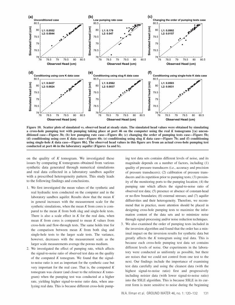
We also use this validation approach on the real Ktomograms. For this, we use the various real K tomo-grams (Figures 3b to 8b) and simulate an independentcross-hole pumping test with pumping taking place atport 46. Pumping test at port 46 was chosen for validationpurposes because it was not used in the construction ofthe K tomograms, and it is also a pumping test with the

cleanest data. Figures 10a to 10f show the results of thiscomparison. According to this figure, the data pairs arescattered along the 45� line, indicating that predictedhead distributions generally are statistically unbiased incomparison with the observed except for those generatedwith a low pumping rate (i.e., the results with low signal-to-noise ratio) (Figure 10b). This plot and the quantitativemeasures (L1 and L2 norms) show that the comparison isconsistently very good, providing us with further confi-dence that SSLE can provide an unbiased estimation ofthe head distribution. Note that the simulated heads willnot necessarily match the observed ones perfectly as theyshould, due to the fact that the tomograms are conditionaleffective K fields and also due to noise in theobservations.

Findings and ConclusionsThe subsurface is inherently heterogeneous at multi-

ple scales, but the delineation of subsurface heterogeneityusing current technology such as with traditional geostat-istical methods is time consuming and expensive. Wepresented here an application of hydraulic tomographyusing cross-hole pumping tests conducted in a laboratoryaquifer to investigate practical issues that may be of con-cern to field hydrogeologists. The main objectives of thisstudy were to examine the role of pumping rate, whichhas a large impact on signal-to-noise ratio, the order of testdata included in the SSLE algorithm, and conditioning

Observed Head (cm)

Sim

ula

ted

hea

d (

cm)

Sim

ula

ted

hea

d (

cm)

78 78.5 79 79.5 80 80.5

Observed Head (cm)78 78.5 79 79.5 80 80.5

Observed Head (cm)78 78.5 79 79.5 80 80.5

Observed Head (cm)78 78.5 79 79.5 80 80.5

Observed Head (cm)78 78.5 79 79.5 80 80.5

Observed Head (cm)78 78.5 79 79.5 80 80.5

78

78.5

79

79.5

80

80.5

Sim

ula

ted

hea

d (

cm)

78

78.5

79

79.5

80

80.5

Sim

ula

ted

hea

d (

cm)

78

78.5

79

79.5

80

80.5

Sim

ula

ted

hea

d (

cm)

78.5

78

79

79.5

80

80.5

78

78.5

79

79.5

80

80.5

Sim

ula

ted

hea

d (

cm)

78

78.5

79

79.5

80

80.5L1: 0.0207L2: 0.0034

L1: 0.0207L2: 0.0034

a)

d)

Unconditioned case

L1: 0.0076L2: 0.0005

Conditioning using core K data case

L1: 0.0160L2: 0.0028

Conditioning using slug K data case

L1: 0.0155L2: 0.0029

Conditioning using single-hole K data case

L1: 0.0379L2: 0.0094

c)

f)

Changing the order of pumping tests caseb)

e)

Low pumping rate case

Figure 9. Scatter plots of simulated vs. observed head at steady state. The simulated head values were obtained by simulatinga cross-hole pumping test with pumping taking place at port 46 on the computer using the synthetic K tomograms [(a) uncon-ditioned case—Figure 3a; (b) low pumping rate case—Figure 4a; (c) changing the order of pumping tests case—Figure 5a; (d)conditioning using core K data case—Figure 6a; (e) conditioning using slug K data case—Figure 7a; and (f) conditioning usingsingle-hole K data case—Figure 8a]. The observed head values in this figure were obtained by simulating the same cross-holetest using the true K field (Figure 2).


on the quality of K tomogram. We investigated theseissues by comparing K tomograms obtained from varioussynthetic data generated through numerical simulationsand real data collected in a laboratory sandbox aquiferwith a prescribed heterogeneity pattern. This study leadsto the following findings and conclusions.

1. We first investigated the mean values of the synthetic and

real hydraulic tests conducted on the computer and in the

laboratory sandbox aquifer. Results show that the mean K

in general increases with the measurement scale for the

synthetic simulations, when the mean K from cores is com-

pared to the mean K from both slug and single-hole tests.

There is also a scale effect in K for the real data, when

mean K from cores is compared to mean K values from

cross-hole and flow-through tests. The same holds true for

the comparison between mean K from both slug and

single-hole tests to the larger scale tests. The variance,

however, decreases with the measurement scale as the

larger scale measurements average the porous medium.

2. We investigated the effect of pumping rate, which affects

the signal-to-noise ratio of observed test data on the quality

of the computed K tomogram. We found that the signal-

to-noise ratio is not as important for the synthetic case but

very important for the real case. That is, the computed K

tomogram was clearer (and closer to the reference K tomo-

gram) when the pumping test was conducted at a higher

rate, yielding higher signal-to-noise ratio data, when ana-

lyzing real data. This is because different cross-hole pump-

ing test data sets contains different levels of noise, and its

magnitude depends on a number of factors, including (1)

quality of pressure transducers (i.e., accuracy and precision

of pressure transducers); (2) calibration of pressure trans-

ducers and its repetition prior to pumping tests; (3) proxim-

ity of the monitoring ports to the pumping location; (4) the

pumping rate which affects the signal-to-noise ratio of

observed test data; (5) presence or absence of constant-head

or no-flow boundaries; (6) external stresses; and (7) aquifer

diffusivities and their heterogeneity. Therefore, we recom-

mend that in practice, more attention should be placed in

designing cross-hole pumping tests to maximize the infor-

mation content of the data sets and to minimize noise

through signal-processing and/or noise reduction techniques.

3. We also examined the order of pumping tests included in

the inversion algorithm and found that the order has a min-

imal impact on the inversion results for synthetic data but

greatly affects the K tomogram using real data. This is

because each cross-hole pumping test data set contains

different levels of noise. Our experiments in the labora-

tory were conducted as uniformly as possible, but there

are noises that we could not control from one test to the

next. Our findings include the importance of examining

test data carefully and using the cleanest data (with the

highest signal-to-noise ratio) first and progressively

including noisier data (with lower signal-to-noise ratio)

into the SSLE algorithm. This is because SSLE in its cur-

rent form is more sensitive to noise during the beginning

Observed Head (cm)

Sim

ula

ted

hea

d (

cm)

78 78.5 79 79.5 80 80.5

Observed Head (cm)78 78.5 79 79.5 80 80.5

Observed Head (cm)78 78.5 79 79.5 80 80.5

Observed Head (cm)78 78.5 79 79.5 80 80.5

Observed Head (cm)78 78.5 79 79.5 80 80.5

Observed Head (cm)78 78.5 79 79.5 80 80.5

78

78.5

79

79.5

80

80.5

Sim

ula

ted

hea

d (

cm)

78

78.5

79

79.5

80

80.5

Sim

ula

ted

hea

d (

cm)

78

78.5

79

79.5

80

80.5

Sim

ula

ted

hea

d (

cm)

78

78.5

79

79.5

80

80.5

Sim

ula

ted

hea

d (

cm)

78

78.5

79

79.5

80

80.5

Sim

ula

ted

hea

d (

cm)

78

78.5

79

79.5

80

80.5

L1: 0.0552L2: 0.0044

Unconditioned case

Conditioning using core K data case Conditioning using slug K data case Conditioning using single-hole K data case

Low pumping rate case Changing the order of pumping tests case

L1: 0.179L2: 0.047

L1: 0.0992L2: 0.0157

L1: 0.0562L2: 0.0037

L1: 0.0437L2: 0.0024

L1: 0.0503L2: 0.0031

(a) (b) (c)

(d) (e) (f)

Figure 10. Scatter plots of simulated vs. observed head at steady state. The simulated head values were obtained by simulatinga cross-hole pumping test with pumping taking place at port 46 on the computer using the real K tomograms [(a) uncon-ditioned case—Figure 3b; (b) low pumping rate case—Figure 4b; (c) changing the order of pumping tests case—Figure 5b;(d) conditioning using core K data case—Figure 6b; (e) conditioning using slug K data case—Figure 7b; and (f) conditioningusing single-hole K data case—Figure 8b]. The observed head values in this figure are from an actual cross-hole pumping testconducted at port 46 in the laboratory aquifer (Figures 1a and b).


stages of K tomogram computation. This sensitivity is due

to the uniform convergence criteria used for sequentially

inverting all pumping test data. One improvement that

could be made to the SSLE algorithm is to include an

option for variable convergence criteria to account for dif-

ferent pumping tests with different noise levels. Further-

more, when hydraulic tomography is conducted using

field data with SSLE in its current form, we recommend

that the cleanest data be included into the SSLE algorithm

first and progressively including noisier data.

4. Conditioning has been thought to help constrain inverse

modeling results. We found that this is certainly the case for

synthetic test data when using the SSLE algorithm. How-

ever, this study shows that the conditioning data itself can

be subject to errors and so conditioning may not necessarily

help in obtaining an improved solution. In particular, condi-

tioning with data that are corrupted with noise can actually

worsen the quality of the K tomograms. Therefore, we rec-

ommend that more attention should be paid to collection of

better conditioning data and minimization of its errors.

5. We also examined the type of data used to conduct the

conditioning of K tomograms. In this paper, we used syn-

thetic and real core, slug, and single-hole K estimates.

Our study showed that core data (assuming that they can

be accurately obtained) improved both synthetic and real

K tomograms. Conditioning of the K tomogram with slug

and single-hole K estimates smoothed the K tomograms

for this sandbox due to the larger support volume associ-

ated with these tests in comparison to the numerical grid

used to compute the K tomograms. Therefore, we recom-

mend scrutinizing the data type used to do the condition-

ing as not all data are created equally. Furthermore, we

recommend that one should consider the support volume

of data used to condition the K tomogram as it can have

an impact on the resolution of the K tomogram.

AcknowledgmentsThis research was supported by the Strategic Envi-

ronmental Research & Development Program (SERDP)under project ER-1365 as well as by funding from theNational Science Foundation (NSF) through grants EAR-0229713, IIS-0431069, and EAR-0450336. The inversioncode used in this analysis is developed by our collabora-tor at the University of Arizona, Tian-Chyi J. Yeh and hisstudents, under a collaborative project funded by SERDPand NSF. We thank Tian-Chyi J. Yeh for his review of theinitial version of the manuscript, and also thank the threeanonymous reviewers for their constructive comments,which have improved the manuscript.

ReferencesBohling, G.C., X. Zhan, J.J. Butler Jr., and L. Zheng. 2002.

Steady shape analysis of tomographic pumping tests forcharacterization of aquifer heterogeneities. Water Re-sources Research 38, no. 12: 1324, doi: 10.1029/2001WR001176.

Bouwer, H., and R.C. Rice. 1976. A slug test for determininghydraulic conductivity of unconfined aquifers with com-

pletely or partially penetrating wells. Water ResourcesResearch 12, no. 3: 423–428.

Brauchler, R., R. Liedl, and P. Dietrich. 2003. A travel timebased hydraulic tomographic approach. Water ResourcesResearch 39, no. 12: 1370, doi: 10.1029/2003WR002262.

Butler J.J., C.D. McElwee, G.C. Bohling. 1999. Pumping tests innetworks of multilevel sampling wells: Motivation and meth-odology.Water Resources Research 35, no. 11: 3553–3560.

Craig, A.J. 2005. Measurement of hydraulic parameters at mul-tiple scales in two synthetic heterogeneous aquifers con-structed in the laboratory. M.S. thesis, Department of Civiland Environmental Engineering, The University of Iowa.

Gottlieb, J., and P. Dietrich. 1995. Identification of the perme-ability distribution in soil by hydraulic tomography. InverseProblems 11, no. 2: 353–360.

Illman, W.A. 2006. Strong field evidence of directional perme-ability scale effect in fractured rock. Journal of Hydrology319, no. 1–4: 227–236.

Illman, W.A., and S.P. Neuman. 2003. Steady-state analyses ofcross-hole pneumatic injection tests in unsaturated frac-tured tuff. Journal of Hydrology 281, no. 1–2: 36–54.

Illman, W.A., and S.P. Neuman. 2001. Type-curve interpretationof a cross-hole pneumatic test in unsaturated fractured tuff.Water Resources Research 37, no. 3: 583–604.

Illman, W.A., X. Liu, and A. Craig. 2007. Steady-state hydraulictomography in a laboratory aquifer with deterministicheterogeneity: Multi-method and multiscale validation ofhydraulic conductivity tomograms. Journal of Hydrology341, no. 3–4: 222–234.

Illman, W.A., and D.M. Tartakovsky. 2006. Asymptotic analysisof cross-hole hydraulic tests in fractured granite. GroundWater 44, no. 4: 555–563.

Klute, A., and C. Dirksen. 1986. Chapter 28: Hydraulic conductiv-ity and diffusivity: Laboratory methods. In Methods ofSoil Analysis, Part 1-Physical and Mineralogical Methods,2nd edition, ed. A. Klute, 687–734. American Society ofAgronomy Inc.

Liu, S., T.-C.J. Yeh, and R. Gardiner. 2002. Effectiveness ofhydraulic tomography: Sandbox experiments. Water Re-sources Research 38, no. 4: doi: 10.1029/2001WR000338.

Liu, X., W.A. Illman, A.J. Craig, J. Zhu ,and T.-C.J. Yeh. 2007.Laboratory sandbox validation of transient hydraulic tomo-graphy. Water Resources Research 43, no. 5: W05404, doi:10.1029/2006WR005144.

McDermott C.I., M. Sauter, and R. Liedl. 2003. New experi-mental techniques for pneumatic tomographical determina-tion of the flow and transport parameters of highlyfractured porous rock samples. Journal of Hydrology, 278,no. 1–4: 51–63.

Vesselinov, V.V., S.P. Neuman, and W.A. Illman. 2001. Three-dimensional numerical inversion of pneumatic cross-holetests in unsaturated fractured tuff: 2. Equivalent parameters,high-resolution stochastic imaging and scale effects. WaterResources Research 37, no. 12: 3019–3042.

Wu, C.-M., T.-C.J. Yeh, J. Zhu, T.H. Lee, N.-S. Hsu, C.-H. Chenand A. Folch Sancho. 2005. Traditional analysis of aquifertests: Comparing apples to oranges? Water ResourcesResearch 41, no. 9: W09402, doi: 10.1029/2004WR003717.

Yeh, T.-C.J., and S. Liu. 2000. Hydraulic tomography: Develop-ment of a new aquifer test method. Water ResourcesResearch 36, no. 8: 2095–2105.

Yeh, T.-C.J., R. Srivastava, A. Guzman, and T. Harter. 1993. Anumerical model for water flow and chemical transport invariably saturated porous media. Ground Water, 31, no. 4:634–644.

Zhu, J., and T.-C.J. Yeh. 2006. Analysis of hydraulic tomogra-phy using temporal moments of drawdown recovery data.Water Resources Research 42, no. 2: W02403, doi:10.1029/2005WR004309.

Zhu, J., and T.-C.J. Yeh. 2005. Characterization of aquiferheterogeneity using transient hydraulic tomography. WaterResources Research 41, no. 7: W07028, doi:10.1029/2004WR003790.


Practical Issues in Imaging Hydraulic Conductivity through Hydraulic Tomography

Documents

Transcript of Practical Issues in Imaging Hydraulic Conductivity through Hydraulic Tomography