Journal of Hydrology (2007) 341, 222–234

ava i lab le at www.sc iencedi rec t . com

journal homepage: www.elsevier .com/ locate / jhydro l

Steady-state hydraulic tomography in a laboratoryaquifer with deterministic heterogeneity:Multi-method and multiscale validation ofhydraulic conductivity tomograms

Walter A. Illman a,b,c,d,*, Xiaoyi Liu a,c, Andrew Craig a

a IIHR-Hydroscience and Engineering, The University of Iowa, Iowa City, IA 52242, USAb Department of Civil and Environmental Engineering, University of Iowa, Iowa City, IA 52242, USAc Department of Geoscience, University of Iowa, Iowa City, IA 52242, USAd Department of Earth and Environmental Sciences, University of Waterloo, Waterloo, Ont., Canada N2L 3G1

Received 30 September 2006; received in revised form 2 March 2007; accepted 7 May 2007

00do

KEYWORDSHydraulic tomography;Pneumatic tomography;Inverse modeling;Model validation;Delineation of subsur-face heterogeneity;Scale effect

22-1694/$ - see front mattei:10.1016/j.jhydrol.2007.05

* Corresponding author. AddE-mail address: walter-illm

r Publis.011

ress: Dean@uiow

Summary Hydraulic tomography potentially is a viable technology that facilitates sub-surface imaging of hydraulic heterogeneity. To date, a comprehensive validation ofhydraulic tomography has not been done either at the laboratory or field scales. The mainobjective of this paper is to examine the accuracy of hydraulic conductivity (K) tomo-grams obtained from the steady-state hydraulic tomography algorithm of [Yeh, T.-C. J.,Liu, S., 2000. Hydraulic tomography: development of a new aquifer test method. WaterResources Research 36, 2095–2105]. We first obtain a reference K tomogram throughthe inversion of synthetic cross-hole test data generated through numerical simulations.The purpose of reference K tomogram generation is to examine the ability of the algo-rithm to image the heterogeneity pattern under optimal conditions without experimentalerrors and with full control of forcing functions (initial and boundary conditions as well assource/sink terms). Parallel to the generation of synthetic data, we conduct hydraulictests at multiple scales in a laboratory aquifer with deterministic heterogeneity to gener-ate data that are used to validate K tomograms from hydraulic tomography. Measurementsinclude multiple K estimates from core, slug, single-hole and cross-hole tests as well asseveral unidirectional, flow-through experiments conducted on the sandbox understeady-state conditions. Validation of K tomograms involved a multi-method and multi-scale approach proposed herein which include: (1) visual comparisons of K tomogramsto the true sand distributions and the reference K tomogram; (2) testing the ability of

hed by Elsevier B.V.

partment of Geoscience, University of Iowa, Iowa City, IA 52242, USA.a.edu (W.A. Illman).

Steady-state hydraulic tomography in a laboratory aquifer with deterministic heterogeneity 223

the K tomogram to predict the hydraulic head distribution of an independent cross-holetest not used in the computation of the K tomogram; (3) comparison of the conditionalmean and variance of local K from the K tomograms to the sample mean and varianceof results from other measurements; (4) comparison of local K values from K tomogramsto those from the reference K tomogram; and (5) comparison of local K values from Ktomograms to those obtained from cores and single-hole tests. The multi-method andmultiscale validation approach proposed herein further illustrates the robustness ofsteady-state hydraulic tomography in subsurface heterogeneity delineation.

Published by Elsevier B.V.

Introduction

The subsurface is heterogeneous at multiple scales and isthe rule rather than the exception. The knowledge of de-tailed three-dimensional distributions of hydraulic conduc-tivity (K) is critical in prediction of contaminant transport,delineation of well catchment zones, and quantification ofgroundwater fluxes including surface-water–groundwaterexchange.

Information about the spatial variability of flow parame-ters is most commonly obtained through inference fromsmall-scale measurements of cores, slug/bail tests, flowme-ter tests and single-hole pressure tests. This requires thedrilling of numerous boreholes and conducting of multiplemeasurements at various depth intervals in each of themusing sophisticated equipment. The approach is expensiveand time consuming. As a consequence, little detailed sitecharacterization has been implemented in practice.

Most recently, tomographic surveys have shown that adetailed heterogeneity distribution can be obtained frommultiple pumping tests using a limited number of boreholes. For example, Illman et al. (1998); (see also Illman(1999) and Illman and Neuman (2001, 2003)) conducted anew type of pneumatic cross-hole test in unsaturated frac-tured tuff. The first unique aspect of these tests was thatthey were conducted sequentially in a tomographic mannerat multiple injection points with a large number of monitor-ing intervals. The second unique aspect of Illman’s (1999)work was the use of multiple injection and observationinterval lengths amounting to cross-hole tests conductedat multiple scales. These cross-hole pneumatic tests werethen analyzed by Vesselinov et al. (2001b) with a three-dimensional numerical inverse model, which amounted toa pneumatic tomography, yielding spatial distributions ofpermeability and porosity. They compared kriged estimatesobtained via simultaneous inversion of three cross-holetests with single-hole permeabilities determined along fourboreholes by Guzman et al. (1996). The correlations weregood in one borehole but not as good in three others. Vess-elinov et al. (2001b) suggested that this may be due to thenumber of pilot points (de Marsily, 1978) used in their inver-sion of the cross-hole test data rather than the number ofmeasurements available from single-hole tests.

Yeh and Liu (2000) developed a sequential geostatisticalinverse method which can be applied to hydraulic tomogra-phy for the interpretation of cross-hole hydraulic tests understeady-state conditions. The main advantage of sequentiallyincluding pumping tests is its computational efficiency. Themethod is based on the sequential successive linear estima-

tor (SSLE) and these authors conducted synthetic simulationsfor 2- and 3-dimensional cases to test their approach. Valida-tion of the steady-state hydraulic tomography was limited toerror-free cases of synthetic simulations.

Liu et al. (2002) conducted a laboratory sandbox study toevaluate the performance of hydraulic tomography in char-acterizing aquifer heterogeneity. This was the first valida-tion study of hydraulic tomography, but the K tomogramswere only visually compared to the distribution of sandtypes and to results from synthetic simulations. The K tomo-grams were not compared to small scale estimates of Kdirectly and the authors explicitly state that the true K dis-tributions were not available for either one of the sand-boxes used in the study. The authors mentioned thaterrors and biases have an effect on their K tomograms,but they did not examine the role of errors and biases di-rectly by isolating their causes.

Other researchers (Gottlieb and Dietrich, 1995; Butleret al., 1999; Bohling et al., 2002; Brauchler et al., 2003;McDermott et al., 2003; Zhu and Yeh, 2005, 2006) havedeveloped methods for interpreting hydraulic and pneu-matic tomography but none of them conducted a detailedvalidation of the K tomograms. Therefore, the main objec-tive of this paper is to examine the accuracy of the K tomo-grams obtained from the steady-state hydraulic tomographyalgorithm developed by Yeh and Liu (2000). We first obtain areference K tomogram through the inversion of syntheticcross-hole test data generated through numerical simula-tions. The purpose of reference K tomogram generation isto examine the ability of the algorithm to image the heter-ogeneity pattern under optimal conditions without experi-mental errors and with full control of forcing functions(initial and boundary conditions as well as source/sinkterms). Parallel to the generation of synthetic data, we con-duct hydraulic tests at multiple scales in a laboratory aqui-fer with deterministic heterogeneity to generate data thatare used to validate the K tomogram from hydraulic tomog-raphy. Measurements include multiple K estimates fromcore, slug, single-hole and cross-hole tests as well as severalunidirectional, flow-through experiments conducted uponthe sandbox under steady-state flow conditions. Validationof K tomograms involved a multi-method and multiscale ap-proach which included: (1) visual comparisons of experi-mental K tomograms (from now on K tomogram) to thetrue sand distributions and the reference K tomogram gen-erated using synthetic pumping test data via numerical sim-ulations (from now on reference K tomogram); (2) testingthe ability of the K tomogram to predict the hydraulic headdistribution of an independent cross-hole test not used inthe computation of the K tomogram; (3) comparison of

224 W.A. Illman et al.

the conditional mean and variance of local K from the Ktomograms to the sample mean and variance of results fromother measurements; (4) comparison of local K values fromK tomograms to those from the reference K tomogram; and(5) comparison of local K values from K tomograms to thoseobtained from cores and single-hole tests. We also examinethe influence of errors and biases on inversion results usingforward and inverse simulations of cross-hole tests. Errorsand biases arising from the conduct of experiments are usu-ally nonexistent in synthetic simulations as implemented byYeh and Liu (2000) and Zhu and Yeh (2005, 2006), so onecannot directly examine their influence. On the other hand,in the field, biases and errors are generally unknown, sotheir influence on the K tomograms cannot be quantified.Therefore, laboratory sandbox studies can be very impor-tant in quantifying the role of errors and biases on the Ktomograms because all the forcing functions (initial/bound-ary conditions; sources/sink terms) can be controlled.

We discuss the sandbox used in the study, providedescriptions of various hydraulic tests conducted in thesandbox for characterization, and discuss methods used toobtain data that will be later used to validate the K tomo-grams. We then discuss the forward and inverse analysesof cross-hole tests, including descriptions of data diagnostictools, inverse modeling results with and without experimen-tal bias and a multi-method/multiscale approach in validat-ing the K tomograms.

Sandbox description

The synthetic heterogeneous aquifer constructed in thesandbox was designed to validate various fluid flow and sol-ute transport algorithms and in particular, the hydraulictomography algorithm. The sandbox is 193.0 cm in length,82.6 cm in height, and has a depth of 10.2 cm. All materialsused inside the sandbox are made of 316 stainless steel,brass, or Viton�. Forty-eight ports, 1.3 cm in diameter, havebeen cut out of the stainless steel wall to allow coring of theaquifer as well as installation of horizontal wells. As thewells have a diameter of 1.3 cm, wall friction effects are

ELEVATION

0.75"

3.25"

3.25"

3.25"

3.25"

3.25"

3.25"

3.25"

3.25"

6.00"

8.00" 5.00"4.25" 10.75"1.9"

75.8"

8.00"

76.00A

A

33.50"

63.50

BUTTRESS

1 2 3

7 8 9

13 14 15

19 20 21

25 26 27

31 32 33

37 38 39

43 44 45

Figure 1 Computer aided design (CAD) drawing of sandbox used fpumped port locations.

considered negligible (at an order of 0.0009 cm) on hydrau-lic tests conducted in the sandbox. Each well was con-structed by making six cuts spaced 1.46 cm apart insections of brass tubing. The cuts were then covered witha stainless steel mesh that was bonded to the tubing withcorrosion resistant epoxy. Extreme care was taken to avoidthe epoxy filling the mesh which could impede water flow.The wells fully penetrate the thickness of the syntheticaquifer. This allowed each location to be monitored by apressure transducer, used as a pumping port and used as awater sampling port. Fig. 1 is a computer aided design(CAD) drawing of the sandbox frontal view, showing the 48port and pressure transducer locations as well as water res-ervoirs for controlling hydraulic head.

The flow system for the sandbox is driven by two con-stant-head reservoirs, one at each end of the sandbox.The adjoining reservoirs are capable of supplying waterthroughout the length and thickness of the sandbox quicklyand efficiently compared to the situation if we had to main-tain an external reservoir alone. The boundary head levelscan be easily adjusted to be equal or to create a desiredhydraulic gradient. We also utilized an intermediate over-flow device to maintain equal constant heads on bothboundaries in the experiments. The device consisted of areservoir with an overflow pipe and tubing connecting itto the inlets at the bottom of the constant head reservoirs.The developed system is also capable of maintaining threeconstant head boundaries simultaneously by ponding waterat the top in addition to fixing the hydraulic heads in thetwo constant head reservoirs.

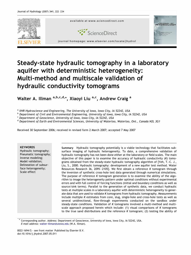
Four different commercially sieved sands [20/30 and4030, U.S. Silica; F-75 and F-85, Unimin Corporation] wereused to pack the sandbox by hand. A special packing toolwas developed to achieve uniform compaction. The sandwas wetted from the bottom and the water levels were in-creased while packing. It was of paramount importance topack the sandbox with a known K distribution in order to val-idate the computed tomogram. The chosen heterogeneitystructure is complex enough so that it provides adequatetesting of various numerical codes. Fig. 2 is a photograph

VIEW

0.75"

5.00" 8.00" 10.75" 4.25" 1.9"8.00"

"

"

BUTTRESS

4 5 6

10 11 12

16 17 18

22 23 24

28 29 30

34 35 36

40 41 42

46 47 48

or the validation of hydraulic tomography. Open circles indicate

Figure 2 Photograph of the sandbox with a deterministicheterogeneous aquifer.

Steady-state hydraulic tomography in a laboratory aquifer with deterministic heterogeneity 225

of the sandbox with the synthetic heterogeneous aquifershowing the different sand types and their distributions.

Discontinuous sand bodies were packed to simulate aheterogeneous aquifer to test the ability of the inverse algo-rithm to delineate sharp contrasts in K. It is also importantto note that the sand distribution was designed to test theeffectiveness of hydraulic tomography to characterize mul-tiple sand grain sizes. Liu et al. (2002) used only two grainsizes to test the effectiveness of the code so the inclusionof four distinct grain sizes would be a stronger test.

The data acquisition system used for the laboratoryexperiments consisted of three major components. Pressuremeasurements were made with 50 Setra model 209 gagepressure transducers with a range of 0–1 psi and a proofpressure of 2 psi, 48 of which measured hydraulic head (h)in the aquifer and one in each constant head reservoir.These pressure transducers were installed at each of the48 data acquisition ports in the stainless steel wall of theflow cell. The second component was a 64-channel dataacquisition board from National Instruments. A hub thatseparates excitation and output currents for the transducerswas assembled at the IIHR-Hydroscience & Engineering ofthe University of Iowa. The third component was a dedi-cated PC with National Instruments LabVIEW software forautomated data acquisition. Further details of the sandboxconstruction and experimental results can be found in Craig(2005).

Sandbox aquifer characterization

Different hydraulic tests were performed in the sandbox tocharacterize the hydrogeologic parameters at multiplescales. We first determined the K of the four types of sandsfrom the extracted core using a constant head permeameter(Klute and Dirksen, 1986). Because the extracted core wasvery small, a special permeameter was built for testing pur-poses. We also conducted slug tests at each of the 48 ports.Due to the small size and configuration of the ports on thesandbox, an external well was attached to the ports insteadof boring vertical wells into the sandbox.

After completing the slug tests, cross-hole tests wereconducted at each of the 46 ports. Two ports were damagedand so we did not conduct cross-hole tests in these ports.The cross-hole tests were conducted by raising the h inthe constant head reservoirs high enough so that waterwas ponded above the sand. The intermediate overflow de-

vice constantly supplied water so that constant h conditionswere maintained at the top and the two side boundaries,while the bottom boundary remained a no-flow boundary.

We also conducted nine unidirectional flow-throughexperiments through the entire sandbox to obtain the effec-tive hydraulic conductivity (Keff) of the entire sandbox un-der steady-state flow conditions. These experiments wereconducted by establishing a constant hydraulic gradientand measuring the discharge through the flow cell.

Description of the forward and inverse models

Forward model

Forward modeling of various hydraulic tests in the sandboxwere done using the two-dimensional water flow and solutetransport code MMOC2 as well as its three-dimensional ver-sion MMOC3 (Yeh et al., 1993). The forward model is capa-ble of simulating water flow and chemical transport throughvariably saturated porous media. The flow equation issolved using the Galerkin finite element technique witheither the Picard or Newton–Raphson iteration scheme.

We also used VSAFT2, a Graphical User Interface (GUI)program based on MMOC2, to obtain equivalent estimatesof hydraulic parameters through manual calibration fromthe slug, single-hole, and cross-hole tests.

Inverse model

Inverse modeling of cross-hole tests in the sandbox wereconducted using a sequential geostatistical inverse ap-proach developed by Yeh and Liu (2000). We only providea brief description of the inversion approach here. Theinverse model assumes a steady flow field and the naturallogarithm of K (lnK) is treated as a stationary stochastic pro-cess. The model additionally assumes that the mean andcorrelation structure of the K field is known a priori. Thealgorithm essentially is composed of two parts. First, thesequential successive linear estimator (SSLE) is employedfor each cross-hole test. The estimator begins by cokrigingthe initial K value determined and observed h collected inone pumping test during the tomographic sequence to cre-ate a cokriged, mean removed ln K (f, i.e., perturbationof ln K) map. We select an initial K obtained from the tradi-tional analysis of pumping test treating the medium to behomogeneous. Cokriging does not take full advantage ofthe observed h values because it assumes a linear relation-ship (Yeh and Liu, 2000) between h and K, while the truerelationship is nonlinear. To circumvent this problem, a lin-ear estimator based on the differences between the simu-lated and observed h values is successively employed toimprove the estimate.

The second step of Yeh and Liu’s (2000) approach is touse the h datasets sequentially instead of simultaneouslyincluding them in the inverse model. In essence, thesequential approach uses the estimated K field and covari-ances, conditioned on previous sets of h measurements asprior information for the next estimation based on a newset of pumping data. This process continues until all thedata sets are fully utilized. Modifications made to the codefor the present study include its ability to account for

226 W.A. Illman et al.

variations in the boundary conditions with each pumpingtest as they are sequentially included and implementingthe modified loop scheme described in Zhu and Yeh (2005).

Estimates of hydraulic conductivity forvalidation of K tomograms

We first determined the K of the four types of sands fromthe horizontal cores obtained during the completion of wellsand port placement. The extracted cores had dimensions of1.28 cm in diameter and 10.16 cm in length. These coreswere then attached to a custom-made constant head per-meameter (Klute and Dirksen, 1986) for determination ofK. Details to the core extraction method and the design ofthe constant head permeameter is provided in Craig(2005). The K values from cores are calculated using Darcy’slaw.

We also conducted slug tests at each of the 48 ports. Dueto the small size and configuration of the ports on the sand-box, an external well was attached to the ports instead ofboring vertical wells into the sandbox. A slug was introducedto perturb the water level in the horizontal well connectedto the port and the corresponding recovery was monitoredusing a pressure transducer. Because existing analyticalsolutions cannot be used to interpret the slug tests withour current setting, we analyzed the data by manually cali-brating VSAFT2 (Yeh et al., 1993), available atwww.hwr.arizona.edu/yeh, by treating the model domainto be a two-dimensional, homogeneous medium (Craig,2005). A fine numerical grid (1.64 cm by 1.64 cm) was devel-oped for the slug test analysis. The numerical simulationswere conducted by raising the initial head at the elementscorresponding to the slugged port and monitoring the corre-sponding decay in the head profile. VSAFT2 was chosen toanalyze the test data for consistency because the code con-tains the forward model used later for hydraulic tomogra-phy. We report the geometric mean of 40 values that wedeem to match the observed data well in Table 1. Resultsobtained revealed that the K values are several orders ofmagnitude smaller than the core values. We suspected thatthe data are affected by skin effects and wellbore storage.In fact, we investigated the issue further by conductingadditional experiments to examine the effects of the num-ber of cuts on the head response to slug tests. In particular,slug tests were conducted in a separate flow cell with tubes

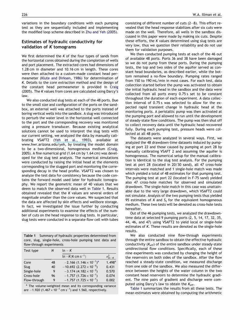
Table 1 Summary of hydraulic properties determined fromcore, slug, single-hole, cross-hole pumping test data andflow-through experiments

Test type N ln � K

ln�KðK cm s�1Þ r2ln�K

Core 48 �2.166 (1.146 · 10�1)a 1.498a

Slug 40 �10.692 (2.272 · 10�5) 0.431Single-hole 9 �3.174 (4.182 · 10�2) 0.570Cross-hole 96 �1.757 (1.726 · 10�1) 0.074Flow-through 9 �1.757 (1.725 · 10�1) 0.002a The volume-weighted mean and its corresponding variance

are �1.920 (1.467 · 10�1 cm s�1) and 1.560, respectively.

consisting of different number of cuts (2–8). This effort re-vealed that the head response stabilizes after six cuts weremade on the well. Therefore, all wells in the sandbox dis-cussed in this paper were made by making six cuts. Despitethese efforts, the K values determined using slug tests arevery low, thus we question their reliability and do not usethem for validation purposes.

We then conducted pumping tests at each of the 46 outof available 48 ports. Ports 36 and 38 have been damagedso we do not pump from these ports. During the pumpingtests, the top and two sides of the aquifer served as con-stant head boundaries, as described earlier, while the bot-tom remained a no-flow boundary. Pumping rates rangedfrom 150 to 190 mL/min in most cases. For each test, datacollection started before the pump was activated to obtainthe initial hydraulic head in the sandbox and the data werecollected from all ports every 0.75 s set to be constantthroughout the duration of each experiment. A data collec-tion interval of 0.75 s was selected to allow for the ex-pected rapid transient change in hydraulic head at themonitoring ports. A peristaltic pump was then activated atthe pumping port and allowed to run until the developmentof steady-state flow conditions. The pump was then shut offto collect recovery data until the hydraulic head recoveredfully. During each pumping test, pressure heads were col-lected at all 48 ports.

The datasets were analyzed in several ways. First, weanalyzed the 48 drawdown-time datasets induced by pump-ing at port 22 and those caused by pumping at port 28 bymanually calibrating VSAFT 2 and assuming the aquifer ishomogeneous. The numerical setup for the manual calibra-tion is identical to the slug test analysis. For the pumpingtest at port 28 (located in 20/30 sand), all 47 cross-holeintervals were matched and 1 single-hole match was madewhich yielded a total of 48 estimates for that pumping test.The pumping test at port 22 (located in F-75 sand) yieldedalso 47 cross-hole matches for observed and simulateddrawdown. The single-hole match in this case was unattain-able due to the very large drawdown, which VSAFT2 couldnot simulate. Analysis of the two pumping tests thus yielded95 estimates of K and Ss for the equivalent homogeneousmedium. These two tests will be denoted as cross-hole testshereafter.

Out of the 46 pumping tests, we analyzed the drawdown-time data at selected 9 pumping ports (2, 5, 14, 17, 32, 35,44, 46, and 47) using VSAFT2 to yield local or single-holeestimates of K. These results are denoted as the single-holeresults.

We also conducted nine flow-through experimentsthrough the entire sandbox to obtain the effective hydraulicconductivity (Keff) of the entire sandbox under steady-stateunidirectional flow conditions. Specifically, each of thesenine experiments was conducted by changing the height ofthe reservoirs on both sides of the sandbox. After the flowreached a steady-state condition, we measured dischargefrom one side of the sandbox. We also measured the differ-ence between the heights of the water column in the twoconstant head reservoirs to determine the hydraulic gradi-ent. The nine pairs of gradient and discharge were com-puted using Darcy’s law to obtain the Keff.

Table 1 summarizes the results from all these tests. Themean estimates were obtained by computing the arithmetic

Steady-state hydraulic tomography in a laboratory aquifer with deterministic heterogeneity 227

mean of the natural logarithm transformed data. The vari-ance was likewise computed using the natural logarithmtransformed data set. We also calculated a volume-weighted mean and variance of the core values which arealso listed in Table 1. The purpose of computing the vol-ume-weighted mean and variance of the core K values wasso that these values are upscaled to the size of the finiteelement grid used for the inversion so that we can comparethem later.

In Table 1, we see that, in general, the mean values ofthe cross-hole and flow-through values coincide in this sand-box, however, core, slug, and single-hole test values arenoticeably smaller suggesting a scale effect. As mentionedearlier, the slug test values are considerably smaller, sowe conclude that near well effects and/or borehole storagedominate the response, causing K estimates to be less reli-able in comparison to other measurements. However, Kestimates from cross-hole tests in the observation well arevery close to the overall K value derived from the flow-through experiments suggesting that these estimates areless affected by near well effects. Therefore, we concludethat the cross-hole observation well data are reliable andwe retain them in our analysis.

Examination of Table 1 also shows that r2lnK

varies fromone type of test to the next with variance decreasing withthe increasing scale. This is because the support volumeof each estimate increases from the core, slug, single-hole,cross-hole and flow-through experiments. As the sample vol-ume increases, K is averaged over the investigated volume.We note that the calculated K values when the medium istreated to be homogeneous are useful, but provide a verylimited resolution of the spatial variability in K. In addition,estimation of equivalent parameters treating the medium tobe homogeneous may yield biased values. This is one impor-tant reason why we conduct hydraulic tomography to deter-mine how the K values vary spatially.

Data diagnostics

Examination of hydraulic head records and theiranimations

Prior to inverse modeling of cross-hole hydraulic tests, weconducted a detailed diagnostic study of the data. Suchdiagnostic tests of data used in forward and inverse modelsare rarely discussed in the literature, but we found that itshould be an integral component to all phases of numericalforward and inverse modeling of cross-hole tests as the useof data corrupted by noise can have a profound effect onmodel results.

We first plotted the transient head records in all 48 portsincluding the two pressure transducers placed in the con-stant head reservoirs to examine the propagation of a pres-sure pulse throughout the aquifer. Plotting of h records inthis manner also allowed us to examine whether the pres-sure transducers were functioning properly as well as toidentify the magnitude of noise during a given cross-holetest. The initial diagnosis of the data revealed that pressuretransducers can be subject to different noise sources includ-ing electrical interference, barometric effects, and minuteuncontrollable variations of the water supply. In general,

the noise can be removed through signal conditioning andde-trending procedures applied to raw data.

We also contoured the initial head distribution within thesandbox to identify whether therewas anywater flowprior tothe cross-hole tests. This also allowed us to study the pres-ence of any drift in pressure transducers. Because the tran-sient head record at a given monitoring port provides onlylimited information about the evolution of the pressure pulsethrough the aquifer during a given pumping test, we alsomade animations of head contours using all head recordsfrom all 48 ports during a given cross-hole test by plottingsuccessive frames of head distributions over the duration ofeach test. This process ensured that each test was conductedcorrectly and gave a pictorial representation of the pressurepropagation throughout the sandbox during a given test.

Diagnostic forward modeling

We next conducted forward modeling of cross-hole tests tofurther diagnose the available data. We assumed that thepumping rate (Q) was deterministic and was accuratelymeasured, the pressure transducers were properly cali-brated and the drift was removed, the boundary conditionsremained stable throughout the experiments and there wasno noise to affect the experimental data. The K values usedin the forward model are those obtained from taking themean value from the core for each type of sand. With theforward model, we then simulate each cross-hole test andcompare the results from the synthetic to the real datathrough a scatter plot.

The forward modeling of the cross-hole tests showedthat the simulated hydraulic head (hs) values are in generalhigher than the measured hydraulic head (hm) values nearthe top and bottom of the sandbox. The head value at thepumped port also differs considerably from the simulationresults, consistently throughout the sandbox. As we arenot aware of the cause(s) of these biases, we conducted adetailed study to determine their cause. A bias can be intro-duced due to the collection of inaccurate data or throughthe misapplication of the forward model.

We first examined all head records carefully. Thisshowed that the initial heads are inconsistent indicatingthe presence of drift in pressure transducers, so we modi-fied the test data to reduce this bias. In particular we ac-counted for pressure transducer drift by calculating thedrawdown (si) at port i, in the following manner:

si ¼ hi;0 � hi ð1Þwhere hi,0 was the initial head at port i during a given cross-hole test and hi is head at port i at time t. We then averagedthe starting hi by taking the arithmetic mean

h0 ¼1

n

Xn

i¼1hi;0 ð2Þ

and used this value as the initial head for all ports. We thensubtracted the si to this starting head to get the modifiedhead for each of the pumping tests.

We also see that the hs are considerably higher than thehm values at the pumping port. The extra head drop can bedue to inertial effects due to a high pumping rate and/or thedevelopment of a low K region at the pumped port (i.e., skineffect). As discussed earlier, a series of diagnostic tests not

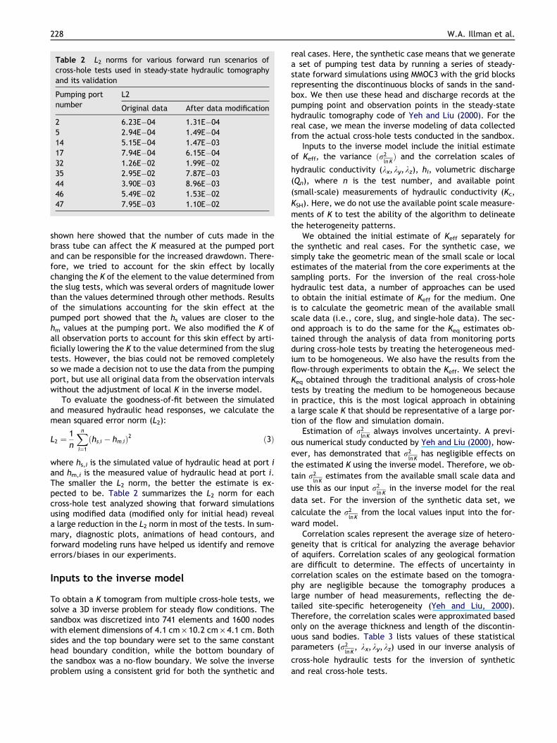
Table 2 L2 norms for various forward run scenarios ofcross-hole tests used in steady-state hydraulic tomographyand its validation

Pumping portnumber

L2

Original data After data modification

2 6.23E�04 1.31E�045 2.94E�04 1.49E�0414 5.15E�04 1.47E�0317 7.94E�04 6.15E�0432 1.26E�02 1.99E�0235 2.95E�02 7.87E�0344 3.90E�03 8.96E�0346 5.49E�02 1.53E�0247 7.95E�03 1.10E�02

228 W.A. Illman et al.

shown here showed that the number of cuts made in thebrass tube can affect the K measured at the pumped portand can be responsible for the increased drawdown. There-fore, we tried to account for the skin effect by locallychanging the K of the element to the value determined fromthe slug tests, which was several orders of magnitude lowerthan the values determined through other methods. Resultsof the simulations accounting for the skin effect at thepumped port showed that the hs values are closer to thehm values at the pumping port. We also modified the K ofall observation ports to account for this skin effect by arti-ficially lowering the K to the value determined from the slugtests. However, the bias could not be removed completelyso we made a decision not to use the data from the pumpingport, but use all original data from the observation intervalswithout the adjustment of local K in the inverse model.

To evaluate the goodness-of-fit between the simulatedand measured hydraulic head responses, we calculate themean squared error norm (L2):

L2 ¼1

n

Xn

i¼1ðhs;i � hm;iÞ2 ð3Þ

where hs,i is the simulated value of hydraulic head at port iand hm,i is the measured value of hydraulic head at port i.The smaller the L2 norm, the better the estimate is ex-pected to be. Table 2 summarizes the L2 norm for eachcross-hole test analyzed showing that forward simulationsusing modified data (modified only for initial head) reveala large reduction in the L2 norm in most of the tests. In sum-mary, diagnostic plots, animations of head contours, andforward modeling runs have helped us identify and removeerrors/biases in our experiments.

Inputs to the inverse model

To obtain a K tomogram from multiple cross-hole tests, wesolve a 3D inverse problem for steady flow conditions. Thesandbox was discretized into 741 elements and 1600 nodeswith element dimensions of 4.1 cm · 10.2 cm · 4.1 cm. Bothsides and the top boundary were set to the same constanthead boundary condition, while the bottom boundary ofthe sandbox was a no-flow boundary. We solve the inverseproblem using a consistent grid for both the synthetic and

real cases. Here, the synthetic case means that we generatea set of pumping test data by running a series of steady-state forward simulations using MMOC3 with the grid blocksrepresenting the discontinuous blocks of sands in the sand-box. We then use these head and discharge records at thepumping point and observation points in the steady-statehydraulic tomography code of Yeh and Liu (2000). For thereal case, we mean the inverse modeling of data collectedfrom the actual cross-hole tests conducted in the sandbox.

Inputs to the inverse model include the initial estimateof Keff, the variance ðr2

lnKÞ and the correlation scales of

hydraulic conductivity (kx,ky,kz), hi, volumetric discharge

(Qn), where n is the test number, and available point

(small-scale) measurements of hydraulic conductivity (Kc,

KSH). Here, we do not use the available point scale measure-

ments of K to test the ability of the algorithm to delineate

the heterogeneity patterns.We obtained the initial estimate of Keff separately for

the synthetic and real cases. For the synthetic case, wesimply take the geometric mean of the small scale or localestimates of the material from the core experiments at thesampling ports. For the inversion of the real cross-holehydraulic test data, a number of approaches can be usedto obtain the initial estimate of Keff for the medium. Oneis to calculate the geometric mean of the available smallscale data (i.e., core, slug, and single-hole data). The sec-ond approach is to do the same for the Keq estimates ob-tained through the analysis of data from monitoring portsduring cross-hole tests by treating the heterogeneous med-ium to be homogeneous. We also have the results from theflow-through experiments to obtain the Keff. We select theKeq obtained through the traditional analysis of cross-holetests by treating the medium to be homogeneous becausein practice, this is the most logical approach in obtaininga large scale K that should be representative of a large por-tion of the flow and simulation domain.

Estimation of r2lnK

always involves uncertainty. A previ-

ous numerical study conducted by Yeh and Liu (2000), how-

ever, has demonstrated that r2lnK

has negligible effects on

the estimated K using the inverse model. Therefore, we ob-

tain r2lnK

estimates from the available small scale data and

use this as our input r2lnK

in the inverse model for the real

data set. For the inversion of the synthetic data set, we

calculate the r2lnK

from the local values input into the for-

ward model.Correlation scales represent the average size of hetero-

geneity that is critical for analyzing the average behaviorof aquifers. Correlation scales of any geological formationare difficult to determine. The effects of uncertainty incorrelation scales on the estimate based on the tomogra-phy are negligible because the tomography produces alarge number of head measurements, reflecting the de-tailed site-specific heterogeneity (Yeh and Liu, 2000).Therefore, the correlation scales were approximated basedonly on the average thickness and length of the discontin-uous sand bodies. Table 3 lists values of these statisticalparameters (r2

lnK, kx,ky,kz) used in our inverse analysis of

cross-hole hydraulic tests for the inversion of synthetic

and real cross-hole tests.

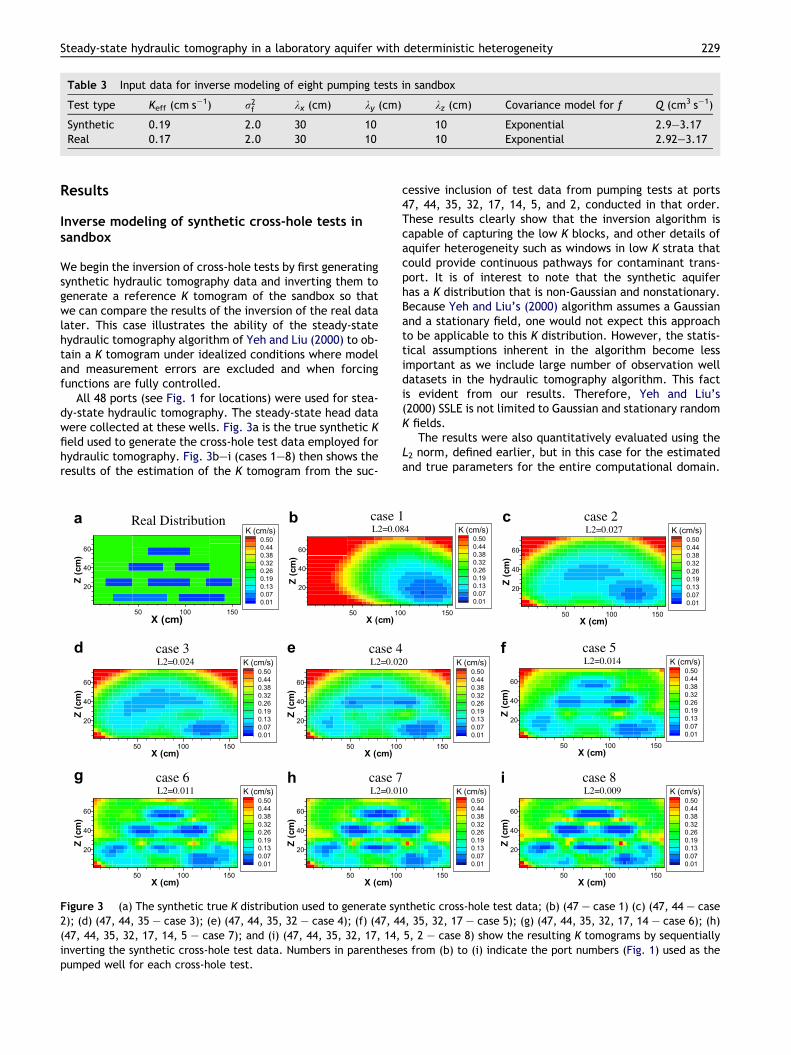
Table 3 Input data for inverse modeling of eight pumping tests in sandbox

Test type Keff (cm s�1) r2f kx (cm) ky (cm) kz (cm) Covariance model for f Q (cm3 s�1)

Synthetic 0.19 2.0 30 10 10 Exponential 2.9–3.17Real 0.17 2.0 30 10 10 Exponential 2.92–3.17

Steady-state hydraulic tomography in a laboratory aquifer with deterministic heterogeneity 229

Results

Inverse modeling of synthetic cross-hole tests insandbox

We begin the inversion of cross-hole tests by first generatingsynthetic hydraulic tomography data and inverting them togenerate a reference K tomogram of the sandbox so thatwe can compare the results of the inversion of the real datalater. This case illustrates the ability of the steady-statehydraulic tomography algorithm of Yeh and Liu (2000) to ob-tain a K tomogram under idealized conditions where modeland measurement errors are excluded and when forcingfunctions are fully controlled.

All 48 ports (see Fig. 1 for locations) were used for stea-dy-state hydraulic tomography. The steady-state head datawere collected at these wells. Fig. 3a is the true synthetic Kfield used to generate the cross-hole test data employed forhydraulic tomography. Fig. 3b–i (cases 1–8) then shows theresults of the estimation of the K tomogram from the suc-

X (cm)

Z(c

m)

50 100 150

20

40

60

K (cm/s)0.500.440.380.320.260.190.130.070.01

a Real Distribution

X (cm)

Z(c

m)

50 10

20

40

60

bL2=0.0case 1

X (cm)

Z(c

m)

50 100 150

20

40

60

K (cm/s)0.500.440.380.320.260.190.130.070.01

dL2=0.024case 3

X (cm)

Z(c

m)

50 100

20

40

60

eL2=0.02case 4

X (cm)

Z(c

m)

50 100 150

20

40

60

K (cm/s)0.500.440.380.320.260.190.130.070.01

gL2=0.011case 6

X (cm)

Z(c

m)

50 100

20

40

60

hL2=0.01case 7

Figure 3 (a) The synthetic true K distribution used to generate sy2); (d) (47, 44, 35 – case 3); (e) (47, 44, 35, 32 – case 4); (f) (47, 4(47, 44, 35, 32, 17, 14, 5 – case 7); and (i) (47, 44, 35, 32, 17, 14,inverting the synthetic cross-hole test data. Numbers in parenthesepumped well for each cross-hole test.

cessive inclusion of test data from pumping tests at ports47, 44, 35, 32, 17, 14, 5, and 2, conducted in that order.These results clearly show that the inversion algorithm iscapable of capturing the low K blocks, and other details ofaquifer heterogeneity such as windows in low K strata thatcould provide continuous pathways for contaminant trans-port. It is of interest to note that the synthetic aquiferhas a K distribution that is non-Gaussian and nonstationary.Because Yeh and Liu’s (2000) algorithm assumes a Gaussianand a stationary field, one would not expect this approachto be applicable to this K distribution. However, the statis-tical assumptions inherent in the algorithm become lessimportant as we include large number of observation welldatasets in the hydraulic tomography algorithm. This factis evident from our results. Therefore, Yeh and Liu’s(2000) SSLE is not limited to Gaussian and stationary randomK fields.

The results were also quantitatively evaluated using theL2 norm, defined earlier, but in this case for the estimatedand true parameters for the entire computational domain.

0 150

K (cm/s)0.500.440.380.320.260.190.130.070.01

84

X (cm)

Z(c

m)

50 100 150

20

40

60

K (cm/s)0.500.440.380.320.260.190.130.070.01

cL2=0.027case 2

150

K (cm/s)0.500.440.380.320.260.190.130.070.01

0

X (cm)

Z(c

m)

50 100 150

20

40

60

K (cm/s)0.500.440.380.320.260.190.130.070.01

fL2=0.014case 5

150

K (cm/s)0.500.440.380.320.260.190.130.070.01

0

X (cm)

Z(c

m)

50 100 150

20

40

60

K (cm/s)0.500.440.380.320.260.190.130.070.01

iL2=0.009case 8

nthetic cross-hole test data; (b) (47 – case 1) (c) (47, 44 – case4, 35, 32, 17 – case 5); (g) (47, 44, 35, 32, 17, 14 – case 6); (h)5, 2 – case 8) show the resulting K tomograms by sequentiallys from (b) to (i) indicate the port numbers (Fig. 1) used as the

230 W.A. Illman et al.

Fig. 3b–i shows that the L2 norm decreases as more pump-ing tests are added, but the rate of reduction diminishes andstabilizes through cases 6–8.

We use the best synthetic result (case 8) as a reference Ktomogram in which we later compare our tomograms fromthe inversion of real cross-hole test data.

Inverse modeling of real cross-hole tests in sandbox

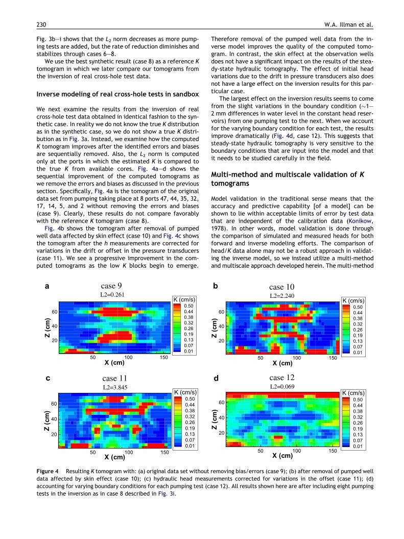
We next examine the results from the inversion of realcross-hole test data obtained in identical fashion to the syn-thetic case. In reality we do not know the true K distributionas in the synthetic case, so we do not show a true K distri-bution as in Fig. 3a. Instead, we examine how the computedK tomogram improves after the identified errors and biasesare sequentially removed. Also, the L2 norm is computedonly at the ports in which the estimated K is compared tothe true K from available cores. Fig. 4a–d shows thesequential improvement of the computed tomograms aswe remove the errors and biases as discussed in the previoussection. Specifically, Fig. 4a is the tomogram of the originaldata set from pumping taking place at 8 ports 47, 44, 35, 32,17, 14, 5, and 2 without removing the errors and biases(case 9). Clearly, these results do not compare favorablywith the reference K tomogram (case 8).

Fig. 4b shows the tomogram after removal of pumpedwell data affected by skin effect (case 10) and Fig. 4c showsthe tomogram after the h measurements are corrected forvariations in the drift or offset in the pressure transducers(case 11). We see a progressive improvement in the com-puted tomograms as the low K blocks begin to emerge.

X (cm)

Z(c

m)

50 100 150

20

40

60

K (cm/s)0.500.440.380.320.260.190.130.070.01

L2=3.845case 11c

X (cm)

Z(c

m)

50 100 150

20

40

60

K (cm/s)0.500.440.380.320.260.190.130.070.01

L2=0.261case 9a

Figure 4 Resulting K tomogram with: (a) original data set withoutdata affected by skin effect (case 10); (c) hydraulic head measuaccounting for varying boundary conditions for each pumping test (ctests in the inversion as in case 8 described in Fig. 3i.

Therefore removal of the pumped well data from the in-verse model improves the quality of the computed tomo-gram. In contrast, the skin effect at the observation wellsdoes not have a significant impact on the results of the stea-dy-state hydraulic tomography. The effect of initial headvariations due to the drift in pressure transducers also doesnot have a large effect on the inversion results for this par-ticular case.

The largest effect on the inversion results seems to comefrom the slight variations in the boundary condition (�1–2 mm differences in water level in the constant head reser-voirs) from one pumping test to the next. When we accountfor the varying boundary condition for each test, the resultsimprove dramatically (Fig. 4d, case 12). This suggests thatsteady-state hydraulic tomography is very sensitive to theboundary conditions that are input into the model and thatit needs to be studied carefully in the field.

Multi-method and multiscale validation of Ktomograms

Model validation in the traditional sense means that theaccuracy and predictive capability [of a model] can beshown to lie within acceptable limits of error by test datathat are independent of the calibration data (Konikow,1978). In other words, model validation is done throughthe comparison of simulated and measured heads for bothforward and inverse modeling efforts. The comparison ofhead/K data alone may not be a robust approach in validat-ing the inverse model, so we instead utilize a multi-methodand multiscale approach developed herein. The multi-method

X (cm)

Z(c

m)

50 100 150

20

40

60

K (cm/s)0.500.440.380.320.260.190.130.070.01

L2=0.069case 12d

X (cm)

Z(c

m)

50 100 150

20

40

60

K (cm/s)0.500.440.380.320.260.190.130.070.01

L2=2.240case 10b

removing bias/errors (case 9); (b) after removal of pumped wellrements corrected for variations in the offset (case 11); (d)ase 12). All results shown here are after including eight pumping

78.5

79

79.5

80

80.5

81

78.5 79 79.5 80 80.5 81

hm (cm)

hs (c

m)

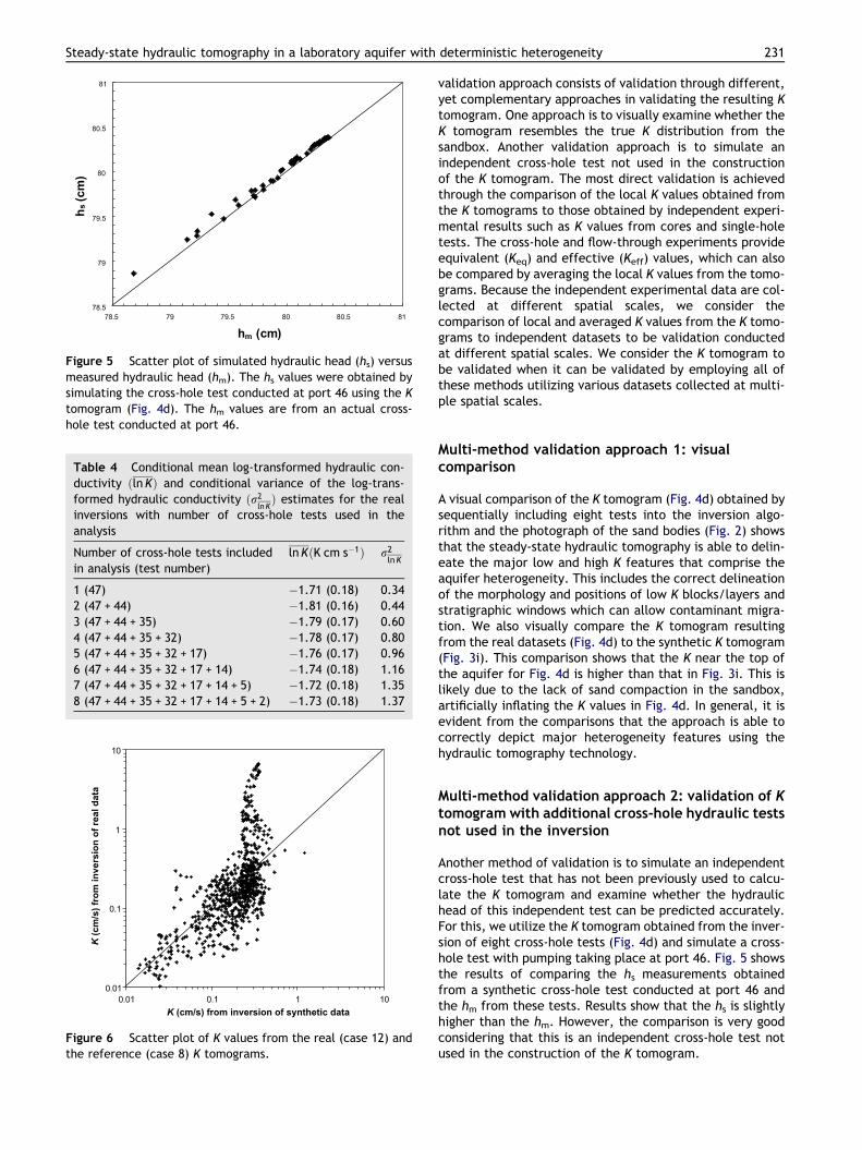
Figure 5 Scatter plot of simulated hydraulic head (hs) versusmeasured hydraulic head (hm). The hs values were obtained bysimulating the cross-hole test conducted at port 46 using the Ktomogram (Fig. 4d). The hm values are from an actual cross-hole test conducted at port 46.

Table 4 Conditional mean log-transformed hydraulic con-ductivity ðlnKÞ and conditional variance of the log-trans-formed hydraulic conductivity ðr2

lnKÞ estimates for the real

inversions with number of cross-hole tests used in theanalysis

Number of cross-hole tests includedin analysis (test number)

lnKðK cm s�1Þ r2ln K

1 (47) �1.71 (0.18) 0.342 (47 + 44) �1.81 (0.16) 0.443 (47 + 44 + 35) �1.79 (0.17) 0.604 (47 + 44 + 35 + 32) �1.78 (0.17) 0.805 (47 + 44 + 35 + 32 + 17) �1.76 (0.17) 0.966 (47 + 44 + 35 + 32 + 17 + 14) �1.74 (0.18) 1.167 (47 + 44 + 35 + 32 + 17 + 14 + 5) �1.72 (0.18) 1.358 (47 + 44 + 35 + 32 + 17 + 14 + 5 + 2) �1.73 (0.18) 1.37

0.01

0.1

1

10

0.01 0.1 1 10K (cm/s) from inversion of synthetic data

K (c

m/s

) fro

m in

vers

ion

of re

al d

ata

Figure 6 Scatter plot of K values from the real (case 12) andthe reference (case 8) K tomograms.

Steady-state hydraulic tomography in a laboratory aquifer with deterministic heterogeneity 231

validation approach consists of validation through different,yet complementary approaches in validating the resulting Ktomogram. One approach is to visually examine whether theK tomogram resembles the true K distribution from thesandbox. Another validation approach is to simulate anindependent cross-hole test not used in the constructionof the K tomogram. The most direct validation is achievedthrough the comparison of the local K values obtained fromthe K tomograms to those obtained by independent experi-mental results such as K values from cores and single-holetests. The cross-hole and flow-through experiments provideequivalent (Keq) and effective (Keff) values, which can alsobe compared by averaging the local K values from the tomo-grams. Because the independent experimental data are col-lected at different spatial scales, we consider thecomparison of local and averaged K values from the K tomo-grams to independent datasets to be validation conductedat different spatial scales. We consider the K tomogram tobe validated when it can be validated by employing all ofthese methods utilizing various datasets collected at multi-ple spatial scales.

Multi-method validation approach 1: visualcomparison

A visual comparison of the K tomogram (Fig. 4d) obtained bysequentially including eight tests into the inversion algo-rithm and the photograph of the sand bodies (Fig. 2) showsthat the steady-state hydraulic tomography is able to delin-eate the major low and high K features that comprise theaquifer heterogeneity. This includes the correct delineationof the morphology and positions of low K blocks/layers andstratigraphic windows which can allow contaminant migra-tion. We also visually compare the K tomogram resultingfrom the real datasets (Fig. 4d) to the synthetic K tomogram(Fig. 3i). This comparison shows that the K near the top ofthe aquifer for Fig. 4d is higher than that in Fig. 3i. This islikely due to the lack of sand compaction in the sandbox,artificially inflating the K values in Fig. 4d. In general, it isevident from the comparisons that the approach is able tocorrectly depict major heterogeneity features using thehydraulic tomography technology.

Multi-method validation approach 2: validation of Ktomogram with additional cross-hole hydraulic testsnot used in the inversion

Another method of validation is to simulate an independentcross-hole test that has not been previously used to calcu-late the K tomogram and examine whether the hydraulichead of this independent test can be predicted accurately.For this, we utilize the K tomogram obtained from the inver-sion of eight cross-hole tests (Fig. 4d) and simulate a cross-hole test with pumping taking place at port 46. Fig. 5 showsthe results of comparing the hs measurements obtainedfrom a synthetic cross-hole test conducted at port 46 andthe hm from these tests. Results show that the hs is slightlyhigher than the hm. However, the comparison is very goodconsidering that this is an independent cross-hole test notused in the construction of the K tomogram.

0.01

0.1

1

0.01 0.1 1K (cm/s) from cores

K (c

m/s

) fro

m in

vers

ion

of re

al d

ata

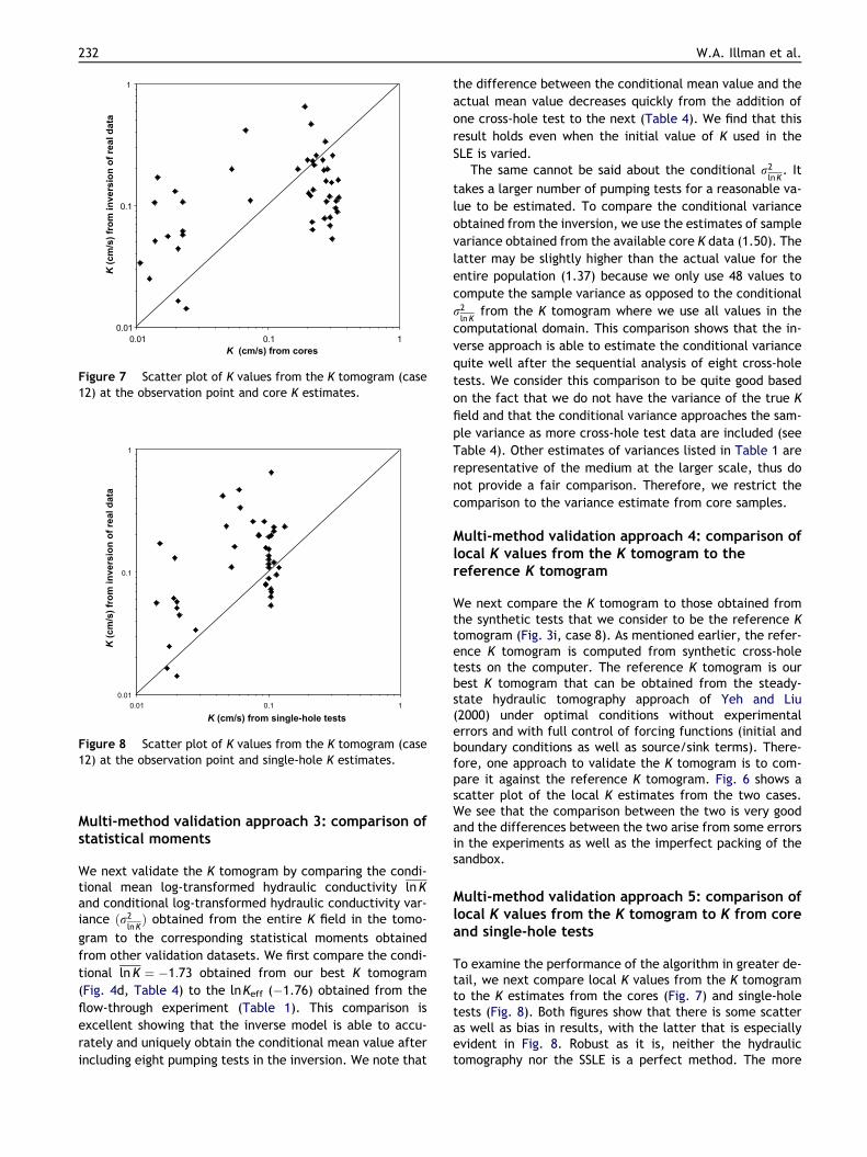
Figure 7 Scatter plot of K values from the K tomogram (case12) at the observation point and core K estimates.

0.01

0.1

1

0.01 0.1 1

K (cm/s) from single-hole tests

K (c

m/s

) fro

m in

vers

ion

of re

al d

ata

Figure 8 Scatter plot of K values from the K tomogram (case12) at the observation point and single-hole K estimates.

232 W.A. Illman et al.

Multi-method validation approach 3: comparison ofstatistical moments

We next validate the K tomogram by comparing the condi-tional mean log-transformed hydraulic conductivity lnKand conditional log-transformed hydraulic conductivity var-iance ðr2

lnKÞ obtained from the entire K field in the tomo-

gram to the corresponding statistical moments obtained

from other validation datasets. We first compare the condi-

tional lnK ¼ �1:73 obtained from our best K tomogram

(Fig. 4d, Table 4) to the lnKeff (�1.76) obtained from the

flow-through experiment (Table 1). This comparison is

excellent showing that the inverse model is able to accu-

rately and uniquely obtain the conditional mean value after

including eight pumping tests in the inversion. We note that

the difference between the conditional mean value and the

actual mean value decreases quickly from the addition of

one cross-hole test to the next (Table 4). We find that this

result holds even when the initial value of K used in the

SLE is varied.The same cannot be said about the conditional r2

lnK. It

takes a larger number of pumping tests for a reasonable va-

lue to be estimated. To compare the conditional variance

obtained from the inversion, we use the estimates of sample

variance obtained from the available core K data (1.50). The

latter may be slightly higher than the actual value for the

entire population (1.37) because we only use 48 values to

compute the sample variance as opposed to the conditional

r2lnK

from the K tomogram where we use all values in the

computational domain. This comparison shows that the in-

verse approach is able to estimate the conditional variance

quite well after the sequential analysis of eight cross-hole

tests. We consider this comparison to be quite good based

on the fact that we do not have the variance of the true K

field and that the conditional variance approaches the sam-

ple variance as more cross-hole test data are included (see

Table 4). Other estimates of variances listed in Table 1 are

representative of the medium at the larger scale, thus do

not provide a fair comparison. Therefore, we restrict the

comparison to the variance estimate from core samples.

Multi-method validation approach 4: comparison oflocal K values from the K tomogram to thereference K tomogram

We next compare the K tomogram to those obtained fromthe synthetic tests that we consider to be the reference Ktomogram (Fig. 3i, case 8). As mentioned earlier, the refer-ence K tomogram is computed from synthetic cross-holetests on the computer. The reference K tomogram is ourbest K tomogram that can be obtained from the steady-state hydraulic tomography approach of Yeh and Liu(2000) under optimal conditions without experimentalerrors and with full control of forcing functions (initial andboundary conditions as well as source/sink terms). There-fore, one approach to validate the K tomogram is to com-pare it against the reference K tomogram. Fig. 6 shows ascatter plot of the local K estimates from the two cases.We see that the comparison between the two is very goodand the differences between the two arise from some errorsin the experiments as well as the imperfect packing of thesandbox.

Multi-method validation approach 5: comparison oflocal K values from the K tomogram to K from coreand single-hole tests

To examine the performance of the algorithm in greater de-tail, we next compare local K values from the K tomogramto the K estimates from the cores (Fig. 7) and single-holetests (Fig. 8). Both figures show that there is some scatteras well as bias in results, with the latter that is especiallyevident in Fig. 8. Robust as it is, neither the hydraulictomography nor the SSLE is a perfect method. The more

Steady-state hydraulic tomography in a laboratory aquifer with deterministic heterogeneity 233

head observations are collected, the higher the resolutionof the estimates will be (i.e., there is no optimum).

Likewise, K estimates from core and single-hole tests arenot devoid of errors contributing to the scatter in Figs. 7 and8. In addition, inaccurate head observations and hydraulicproperty measurements (i.e., noise) during HT can unequiv-ocally lead to an inaccurate estimate or cause the estimatesto become unstable. The SSLE can overcome the impacts ofnoise through loosening of convergence criteria, but thiscauses the estimates to become smoother, which effec-tively results in a loss of information gained from thehydraulic head records.

Discussion

While the validation of hydraulic and pneumatic tomogra-phy under field conditions is our ultimate goal, the valida-tion of hydraulic tomography and other tomographytechnologies in the laboratory is very important and a nec-essary step. In the laboratory, we are better able to controlthe forcing functions fully and quantify the errors. We canalso pack a heterogeneous structure that is almost fully pre-scribed. However, the true K field remains unknown becauseof packing variations. In addition, there are only a finitenumber of small scale samples that can be used for valida-tion purposes. Therefore, we emphasize that even in thelaboratory setting, a direct and complete validation of re-sults is generally difficult.

In this study, we have shown that the K tomogram can bevalidated using multiple methods. The tomograms can alsobe validated at multiple scales from the smaller scale, inwhich the local K values are compared to core and single-hole K estimates to the larger-scale K estimates from othercross-hole and flow-through experiments. Such a multi-fac-eted approach in validation adds more confidence on theability of the algorithm to tackle field scale problems.

One form of model validation involves the establishmentof greater confidence in a given model by conducting simu-lations of datasets that have not been used for calibrationpurposes. For example, one can calibrate a model usingone set of pumping test data. If the calibrated model fromthis first pumping test can predict system response accu-rately in a second pumping test (e.g., conducted using an-other well), one can have greater confidence in thecalibrated model. On the other hand, if the parametersneed to be adjusted to match the response of the 2nd pump-ing test, the process becomes a second calibration and addi-tional datasets are needed to continue with the validationexercise. Model validation is complete when the validationdatasets are matched against simulated values resultingfrom the previously calibrated parameter values.

This is precisely the essence of hydraulic tomographyconducted with sequential inclusion of data. Therefore, itamounts to a repeated validation of the estimated K fieldwith new datasets that are sequentially added. The methodis robust, but it is not the panacea technology. This is be-cause the computed K tomogram is non-unique as thereare an infinite number of solutions to the steady-state in-verse problem for a heterogeneous K field, even when allof the forcing functions are fully specified. Only when dataare available at all estimated locations will the inverse

problem be well-posed and ultimately lead to a unique solu-tion (e.g., Yeh et al., 1996; Yeh and Liu, 2000; Liu et al.,2002 and Yeh and Simunek, 2002). This is not the case here.However, it is important to recognize that we have obtaineda solution to the inverse problem that is consistent with theheterogeneity patterns that we can visualize and directlycompare against the experimentally packed sand distribu-tions (Fig. 2). In addition, we were able to validate theresulting K tomogram using multiple methods and at multi-ple scales so our approach provides more confidence in thesolution of the inverse problem.

Earlier, we saw that errors and biases can be very impor-tant in the result of the K tomogram and the blind additionof new data does not mean that it will automatically gener-ate better results. Therefore, more effort should be ex-pended on collecting accurate data and additionalresearch should be conducted on improving hydraulictomography technology both in sandbox experiments andin the field. This study also emphasizes the importance ofreducing experimental errors and biases during validationof traditional groundwater flow and contaminant transportmodels.

Summary

Hydraulic tomography is a technology that facilitates theimaging of subsurface heterogeneity in hydraulic parame-ters. To date, a comprehensive validation of the hydraulicconductivity (K) tomogram has not been done either atthe laboratory or field scales. Previous laboratory investiga-tions assumed that packing was perfect and in general,small scale data were not available for a direct comparison.This study provides the first such examination using small-scale K data obtained from cores and single-hole tests aswell as large-scale K estimates obtained from flow-throughexperiments in a sandbox with deterministic heterogeneityin hydraulic parameters.

Prior to inverse modeling of data, we conducted a de-tailed diagnostic study to investigate the magnitude andcause of errors and biases in data through scatter plots, con-tour plots and data animations. Such diagnostic tests of dataused in forward and inverse models are rarely discussed inthe literature, but we found that it should be an integralcomponent of all phases of numerical forward and inversemodeling of cross-hole tests as the use of data corruptedby noise can have a profound effect on both forward and in-verse model results.

Validation of the K tomograms involved a multi-methodand multiscale approach which included: (1) visual compar-isons of K tomograms to the true sand distributions as wellas to the reference K tomogram; (2) testing the ability ofthe K tomogram to predict the hydraulic head distributionof an independent cross-hole test not used in the computa-tion of the K tomogram; (3) comparison of the conditionalmean and variance of local K from the K tomograms tothe sample mean and variance of results from other mea-surements; (4) comparison of local K values in K tomogramsto those from the reference tomogram; and (5) comparisonof local K values in K tomograms to those obtained fromcores and single-hole tests. The multi-method and multi-scale validation approach proposed herein further illus-

234 W.A. Illman et al.

trates the robustness of hydraulic tomography in subsurfaceheterogeneity delineation.

Previously, the effects of errors and biases on the Ktomograms have not been investigated in detail. Thesteady-state inversion of cross-hole tests in a synthetic lab-oratory aquifer showed that the approach is sensitive to er-rors and biases. Data diagnostics combined with forwardmodeling provided valuable insight into identifying thecause of such errors and biases. Specifically, the errors iden-tified include drift in pressure transducer readings, a skineffect influencing hydraulic head at the pumped well, andinaccurate treatment of boundary conditions, among oth-ers. We found that accurate modeling of boundary condi-tions is essential in conducting steady-state hydraulictomography and obtaining accurate K tomograms. In realfield situations, the boundary conditions of the field siteneed to be studied carefully through forward modelingand better site characterization. Further research is clearlyneeded to improve hydraulic tomography technology both inthe laboratory and under field conditions.

Acknowledgements

This research was supported by the Strategic Environmen-tal Research & Development Program (SERDP) as well asby funding from the National Science Foundation (NSF)through Grants EAR-0229713, IIS-0431069, and EAR-0450336. The inversion code used in this analysis is devel-oped by our collaborator at the University of Arizona, Tian-Chyi J. Yeh and his students, under a collaborative projectfunded by NSF and SERDP. We thank Junfeng Zhu and Tian-Chyi J. Yeh for their assistance in using the steady-statehydraulic tomography code. We also thank Mike Kundertof IIHR-Hydroscience & Engineering for drafting Fig. 1. Fi-nally, we greatly appreciate the constructive commentsmade by the anonymous reviewers which improved themanuscript.

References

Bohling, G.C., Zhan, X., Butler Jr., J.J., Zheng, L., 2002. Steadyshape analysis of tomographic pumping tests for characteriza-tion of aquifer heterogeneities. Water Resources Research 38,1324. doi:10.1029/2001WR001176.

Brauchler, R., Liedl, R., Dietrich, P., 2003. A travel time basedhydraulic tomographic approach. Water Resources Research 39,1370. doi:10.1029/2003WR002262.

Butler, J.J., McElwee, C.D., Bohling, G.C., 1999. Pumping tests innetworks of multilevel sampling wells: Motivation and method-ology. Water Resources Research 35, 3553–3560.

Craig, A.J., 2005. Measurement of hydraulic parameters at multiplescales in two synthetic heterogeneous aquifers constructed inthe laboratory, M.S. thesis, Department of Civil and Environ-mental Engineering, The University of Iowa.

de Marsily, G., 1978. De l’Identification des systemes en hydrogeo-logiques, these de docteur es sciences. Univ. Pierre et MarieCurie-Paris VI, Paris.

Gottlieb, J., Dietrich, P., 1995. Identification of the permeabilitydistribution in soil by hydraulic tomography. Inverse Problems11, 353–360.

Guzman, A.G., Geddis, A.M., Henrich, M.J., Lohrstorfer, C.F.,Neuman, S.P., 1996. Summary of Air Permeability Data FromSingle-Hole Injection Tests in Unsaturated Fractured Tuffs at theApache Leap Research Site: Results of Steady-State Test Inter-pretation, NUREG/CR-6360, U.S. Nucl. Regul. Comm., Washing-ton, DC.

Illman, W.A., 1999. Single- and cross-hole pneumatic injection testsin unsaturated fractured tuffs at the Apache Leap Research Sitenear Superior, Arizona, Ph.D. dissertation, Department ofHydrol. and Water Resour., University of Arizona, Tucson.

Illman, W.A., Neuman, S.P., 2001. Type-curve interpretation of across-hole pneumatic test in unsaturated fractured tuff. WaterResources Research 37, 583–604.

Illman, W.A., Neuman, S.P., 2003. Steady-state analyses of cross-hole pneumatic injection tests in unsaturated fractured tuff.Journal of Hydrology 281, 36–54.

Illman, W.A., Thompson, D.L., Vesselinov, V.V., Chen, G., Neuman,S.P., 1998. Single- and Cross-Hole Pneumatic Tests in Unsatu-rated Fractured Tuffs at the Apache Leap Research Site:Phenomenology, Spatial Variability, Connectivity and Scale,NUREG/CR-5559, U.S. Nucl. Regul. Comm., Washington D.C.

Klute, A., Dirksen, C., 1986. Hydraulic conductivity and diffusivity:laboratory methods. In: Klute, A. (Ed.), Methods of Soil AnalysisPart 1 – Physical and Mineralogical Methods, second ed.American Society of Agronomy, Inc. (Chapter 28).

Konikow, L., 1978. Calibration of ground-water models. In: Verifi-cation of Mathematical and Physical Models in Hydraulic Engi-neering. American Society of Civil Engineers, New York, pp. 87–93.

Liu, S., Yeh, T.-C.J., Gardiner, R., 2002. Effectiveness of hydraulictomography: sandbox experiments. Water Resources Research38. doi:10.1029/2001WR000338.

McDermott, C.I., Sauter, M., Liedl, R., 2003. New experimentaltechniques for pneumatic tomographical determination of theflow and transport parameters of highly fractured porous rocksamples. Journal of Hydrology 278, 51–63.

Vesselinov, V.V., Neuman, S.P., Illman, W.A., 2001b. Three-dimensional numerical inversion of pneumatic cross-hole testsin unsaturated fractured tuff: 2. Equivalent parameters, high-resolution stochastic imaging and scale effects. Water ResourcesResearch 37, 3019–3042.

Yeh, T.-C.J., Srivastava, R., Guzman, A., Harter, T., 1993. Anumerical model for water flow and chemical transport invariably saturated porous media. Ground Water 31,634–644.

Yeh, T.-C.J., Jin, M., Hanna, S., 1996. An iterative stochasticinverse approach: conditional effective transmissivity and headfields. Water Resources Research. 32, 85–92.

Yeh, T.-C.J., Liu, S., 2000. Hydraulic tomography: development ofa new aquifer test method. Water Resources Research 36, 2095–2105.

Yeh, T.-C.J., Simunek, J., 2002. Stochastic fusion of information forcharacterizing and monitoring the vadose zone. Vadose ZoneJournal 1, 207–221.

Zhu, J., Yeh, T.-C.J., 2005. Characterization of aquifer heteroge-neity using transient hydraulic tomography. Water ResourcesResearch 41, W07028. doi:10.1029/2004WR003790.

Zhu, J., Yeh, T.-C.J., 2006. Analysis of hydraulic tomography usingtemporal moments of drawdown recovery data. WaterResources Research 42, W02403. doi:10.1029/2005WR004309.