1

9th European Conference on the Mathematics of Oil Recovery — Cannes, France, 30 August - 2 September 2004

Abstract

This paper presents a fully automated history matching (HM) method for average field and region pressures and for aquifer behaviors. This means that already with a single simulation run the average pressure and water influx is reproduced. The aquifer model, analytical or gridded will not be designed as usual at the beginning but at the end of the HM process.

The applicability of the method was extensively tested on many field cases. Practice showed that usual history matching time could be reduced by a factor of up to 5. The paper contains a detailed description of the method and suggestions for the implementation in any simulation software. By presenting three field cases the strength and applicability of the concept for black oil and compositional models will be shown.

Introduction

Modern reservoir characterization techniques deliver more and more detailed descriptions of the hydrocarbon reservoirs, but do not deal with the aquifers. However, many oil and gas reservoirs have an associated aquifer, forming an integrated hydrodynamic system for which the pressure decline will be strongly influenced by the aquifer. In a conventional history matching (HM) process the first step must be to match the reservoir pressure, which means to determine the aquifer properties. This can be a tedious work, but it is also the wrong approach. The aquifer parameters are highly uncertain and should not have an influence on screening the geological realizations or on tuning the reservoir parameters.

This paper presents a different approach. The aquifer model will be determined and introduced at the end of the HM, well knowing that in most of the cases no unique solution exists. The concept and workflow is as follows: The grid model is split in a productive area (PA) and in an aquifer grid. The PA is divided in an arbitrary number of volume regions. An artificial boundary, which can be segmented, is put outside the water oil contact, preferably at the outer blocks of the PA. Each boundary segment is related to one volume region. The well rates are defined in term of reservoir volumes. Now water will be injected/produced in/from the boundary segment to match the historical region pressures. The method for that is called Target Pressure Method (TPM). The determination of the boundary rates and their distribution between the boundary blocks are not trivial because the volume regions can communicate to each other. Beyond that transient effects must be considered too. Note that if the calculated region pressure is equal with the historical one, then the overall reservoir volume production rate must be also correct, per definition. Thus the history match can be started immediately with matching the oil (or gas) production, water cut, GOR, well pressures and RFT data. All further reservoir parameter changes influence the water influx, but this will be adapted for every run automatically.

If the HM is completed, then based on the calculated “water influx”, the parameters of different analytical aquifer models (Van Everdingen-Hurst, Fetkovich, etc.) are determined for each boundary segment. This step is similar to the one used in material balance calculations. Using the parameters of the analytical models, the gridded aquifer will be designed (size, permeability, effective compressibility, etc.). Both, gridded aquifer model and best analytical model can be used for predictions.

B027 AUTOMATED DETERMINATION OF AQUIFER PROPERTIES FROM FIELD PRODUCTION DATA

Georg M. Mittermeir1, Johannes Pichelbauer2, Zoltán E. Heinemann1

1Department of Petroleum Engineering, University of Leoben, Austria

2RAG, Austria

2

The paper describes the workflow, the target pressure method for prediction of the boundary injection rates, the determination of the optimal analytical aquifer model and a method how to create gridded aquifers. At the end one artificial and two real field examples will be presented. The paper is based on two thesis works, those from Pichelbauer [1] and Mittermeir [2]. The reader can find more details and examples related to the topic in this documents.

Aquifer and Productive Area Domain

Modern reservoir simulators [3] build the grid model separately for the reservoir and the aquifer domains, which will be merged to one grid system. To avoid any confusion we use the expression productive area (PA) instead of “reservoir”. The PA has a greater extension than the hydrocarbon domain, covering some part of the water-saturated formation too. The original idea was to enable the linkage of a PA with a series of aquifer models and vice versa, allowing to run different combinations parallel and to accelerate the HM process. Older commercial packages construct the grid for the whole hydrodynamic system in one step. In such cases the PA grid can be created by deactivating the aquifer grid blocks, and the aquifer model by eliminating the PA blocks.

The only common part of the two independent domains is a row of blocks that links these domains together. By definition this borderline is formed by the outermost row of PA grid blocks and is called artificial boundary. When the aquifer and the PA domains are merged into one full field model such a boundary acts as interface for fluxes and pressures between the two grids. It is important to note that the artificial boundary is located between an edge-water drive aquifer and the PA vertically and not between the reservoir and a bottom-water drive aquifer horizontally. This boundary can be also used to operate the domains independently from each other by applying appropriate boundary conditions. If the water efflux from the aquifer is known it would be possible to operated only the PA grid in combination with the boundary. To mask water encroachment water must be injected into the boundary elements. The injected water must be equal to the amount of water flowing across the boundary if an aquifer grid was present. This will result in a pressure performance corresponding to the full field model. But it is also possible to operate just the aquifer grid. Then production of water must take place from the boundary blocks. For HM purposes it would be beneficial to have a method that calculates water volumes to be injected into the boundary required to match observed field production data, especially field pressure.

Target Pressure Method

The PA itself may consist of an arbitrary number of volume regions. The differentiation can be made either based on geological features like faults and lithology or can be done just arbitrary. The artificial boundary blocks are not part of any volume region. Further, artificial boundaries do not have to be continues, they can be split up into segments. Every boundary segment is assigned to a distinct volume region but they do not have to border the volume regions they belong to.

The historical average pressure of the volume regions, which can be determined for the pore volume or for the hydrocarbon volume as well, shall be known as function of the time. These average pressure functions should be reproduced in all HM runs as close as possible, therefore they are called “target pressures”. The volume region to which a “target pressure” and consequently an artificial boundary segment were assigned, are called “target area”. Note that it is not necessary to define all volume regions as target areas. The calculation scheme of water influx required to match pressures of a target area is called target pressure method or shortly TPM.

Now let us operate the grid model without aquifer. To achieve a match of simulated and the target pressures it is necessary to inject water into the artificial boundary. To determine the right water injection rate is not a trivial issue. Problems regarding practical implementation are:

1) Well bottom hole pressures (i.e. the perforation block pressures) can be quite different and therefore the determination of target production in terms of reservoir volume and so the calculation of the equivalent boundary injection rate is uncertain.

2) Compressibility of the target area can change suddenly around bubble point pressure.

3

9th European Conference on the Mathematics of Oil Recovery — Cannes, France, 30 August - 2 September 2004

3) Water injected into the boundary does not effect immediately the pressure of the hydrocarbon saturated part. This time lag is related to the distance and the permeability.

4) The target areas can communicate with each other. 5) It is possible that target area and corresponding boundary are not connected directly. 6) Due to the water injection the boundary block pressures may exceed the initial pressure. The reason

for that is the low permeability of the boundary area. 7) The injection rate can easily oscillate, making the procedure instable.

To make the explanation simple, at first one should assume the following circumstances: 1) The target area and the corresponding boundary segment are directly connected . 2) The boundary block volume is negligible compared to the volume of the target area. 3) The conductivity between the boundary and the hydrocarbon volume of the target area (water

saturated blocks) is high. 4) The target pressure is defined for reference time points. The time intervals between two reference

points, ∆tp, are considerable longer as the time steps, ∆t, used during the simulation runs.

If conditions 1 to 3 are valid the transient period for the target area will be short. This means if one produces from the target area and injects into the boundary with constant pressures the situation will become steady state and the rates constant after a time period ps tt ∆<∆ . Choosing a time step stt ∆≥∆

for which pttm ∆=∆ , m = 1,2… then the boundary injection rate for the actual time step can be

determined assuming steady state conditions. Let be pn the actual area pressure and 1ˆ +np the target pressure at the end of the time step, then the first guess for the boundary injection rate is:

11

1 ˆ ++

+ +∆−

= nnn

ntww Q

tppCqB . (1)

The average production rate Qn+1 will be calculated for a time period of ∆t in actual reservoir volume as usually, on well-by-well basis. The formation volume factor Bw is calculated for the pressure 1ˆ +jp . The overall compressibility of the target area is in a black oil formulation:

( )i

m

i g

gg

s

o

g

o

oo

w

wwactinit

m

iit dpB

dBS

dpdR

BB

dpBdBS

dpBdBSVMcVCC ∑∑

== ⎥⎥⎦

⎤

⎢⎢⎣

⎡

⎥⎥⎦

⎤

⎢⎢⎣

⎡+⎟⎟

⎠

⎞⎜⎜⎝

⎛−+−+⋅==

1,,

1φφφ , (2)

where M is the rock compaction factor. The summation is done over all blocks belonging to the target area. Ct will be calculated for the pressure pn and 1ˆ +np as well. For 1ˆ +np the saturations can be taken explicit at time n or implicit. Expecting that pressure will change from pn to 1ˆ +np during the time step, the average compressibility will be:

( )nt

nt

nt CCC +⋅= ++ 11 5.0 . (3)

Now the solution can perform for the time step using IMPES or fully implicit scheme, resulting in an average area pressure pn+1

, which will not be equal to 1ˆ +np . If the difference is small than the calculated pressure can be accepted and the next time step can perform, if not the time step must be repeated using a corrected boundary injection rate. The correction can be calculated easily from the pressure failure:

tBppCq

w

nnn

tw ∆−

=∆++

+11

1 ˆ. (4)

The time step can be repeated many times but experiences show that in most cases no iteration is necessary, and also in difficult situations the solution converges in maximum two steps. The procedure can fail in two cases:

1) It is possible that the time step ∆t is too large, which means that the solution does not converge, and therefore the condition ∆t ≥ ts cannot be satisfied. In this case ∆t must be cut in m smaller time steps

4

with the consequence that not only the last time step, but the last m time steps must be repeated with the corrected injection rate. Note that production and boundary injection rates are constant during the m small time steps. Naturally, the stage at the start of the m time steps must be stored.

2) It is also possible that ∆ts > ∆tp, which means that the transient period is long compared to the reference interval. Theoretically such a case could be handled based on the principle of superposition, as introduced by Van Everdingen and Hurst. This means that at a given time it would be necessary to modify the boundary injection rates over more ∆tp intervals backwards. This cannot be practical. Such a situation is an indicator for an improper setup of the productive area grid and can be corrected easily by modifying the grid model. Three possible improvements can be considered. The first is to move the water-injecting boundary closer to the target area. Another possibility is to revise the permeability of the target area. Both modifications will shorten the time lag between water injection at the boundary and arrival of the pressure supporting effect in the target area. The third possibility is to reduce the size of the target area by cutting the reservoir into more volume regions. All three possibilities were successfully tested. The third possibility was applied to Example 3 presented at the end of the paper.

The rate qw has to be distributed among the blocks of the boundary in such a way that the individual boundary block pressures pi converge towards the average boundary pressure p . This is done using a kind of injectivity index Ji valid for the boundary block i,

)( jiji ppJ −= τ if 0>− jpp else 0=iJ , (5)

where j is a non-boundary neighbor to i and τij is the block pair transmissibility of two blocks. p is a weighted average boundary pressure. The weighting factor ω can be either the pore volume of the boundary blocks or the communication surface to the connected region.

∑∑= iii pp ωω (6)

If more non-boundary blocks j border a boundary block i the injectivity indices have to be summed up. If a non-boundary block j neighbors more than one boundary block i the injectivity index has to be reduced accordingly. Finally the water injection during the time step ∆tn+1 for a single boundary block i follow as,

( ) ∑⋅=i

iwiwi JqJq . (7)

Applying this methodology allows to support the different volume regions of the productive area domain with the correct water influx in a way that the simulated region pressures match the historic target pressures. This is guaranteed within the first simulation run already. Since no uncertainties regarding the aquifer region have to be taken into account it could be immediately started to match the model on a well basis. For prediction runs an aquifer model has to be determined exhibiting the same characteristics as the water influx determined by the TPM. Two possibilities exist. The first is to assign an analytical aquifer model to the artificial boundaries and the second is to merge the productive area grid with an appropriate aquifer grid.

Identification of the optimal analytical aquifer model

The target pressure method calculates the water flux across the artificial boundaries and the according boundary pressures as a function of time. This analogues a material balance calculation and can be used in a similar manner to determine the parameters of an analytical aquifer model. Such an analytical aquifer model will reproduce the water influx calculated by the TPM. Thus the already history matched productive area grid model is still valid. To determine the best fitting analytical aquifer model following error function should be minimized:

[ ]2

1)()(∑

=

−=N

n

ne

nn tWtWE ω , (8)

5

9th European Conference on the Mathematics of Oil Recovery — Cannes, France, 30 August - 2 September 2004

where W(tn) is the water influx from the TPM calculation, We(tn) is the water influx from one of the available analytical models, mentioned below, and ωn is a weighting factor based on the elapsed simulation time. It expresses that water influxes taking place at a later time have more importance than early ones. This allows reducing transient effects occurring most likely at early times.

A procedure for determining a best fitting analytical aquifer model was developed. For pseudo-steady state flow conditions parameters describing the analytical aquifer model introduced by Fetkovich [4] will be calculated. For non-steady state flow conditions the parameters of the Van Everdingen-Hurst [5] model, respectively of its modified version published by Vogt and Wang [6] will be determined. For both flow conditions the fitting procedure is done in an iterative way.

Parameter determination for the Fetkovich model

For the Fetkovich model two parameters the productivity index and the maximum encroachable water must be determined. At first absolute minimum values are calculated for them. The calculation of the minimum productivity index is based on an infinite amount of encroachable water and the minimum encroachable water is calculated based on the assumption of an infinite productivity index. Based on these initial values the water influx function given by the analytical model is calculated. Then the cumulative error between water influx of the TPM and the analytical model is calculated. Afterwards the model parameters are increased. Again water influx and error function are calculated. If the error becomes less the parameters are increased again, if the error becomes larger the parameters are decreased so that the new parameters are between the initial and the previous optimization step. This is done until the termination criterion being either a maximum number of iteration steps without improvement in error or reaching an absolute error limit is reached.

Parameter determination for the Vogt-Wang model

For the Vogt-Wang model the search procedure is different. For this model three parameters have to be determined. They are the time conversion factor β, the dimensionless outer aquifer radius reD and an aquifer related constant, C. The number of dimensionless outer aquifer radii is limited. This allows testing all of them. For every radius a dimensionless time conversion factor and aquifer related constant have to be determined. Again the error function has to be minimized. After testing all radii the one with the smallest error describes in combination with its aquifer related constant and time conversion factor the best fitting Vogt-Wang model.

The determination of the time conversion factor and the aquifer related constant go hand in hand. Starting from an initial β an array of equidistant β values is created. Based on these β vales and an aquifer related constant of C=1 an array of water influxes will be calculated. For every entry the actual C can be calculated by

( )∑∑==

=N

n

nAe

nN

n

nSe

nAe

n WWWC1

2,

1,, ωω , (9)

where nAeW , is the cumulative water influx at the n-th time step of the analytical Vogt-Wang solution and

nSeW , is the cumulative water influx from the TPM simulation run. ω is a weighting factor taking into

consideration the elapsed simulation time. Regarding these C values the real water influx of the analytical model can be calculated. Based on this water influx array the β leading to the smallest error can be determined. If this β is located at the lower end of the array then β will be decreased for the next time step. If it is located at the upper end of the array then β will be increased. If the β showing the smallest error is located somewhere between the upper and the lower end, this β will be taken as a starting point for the next iteration. Again an array of β values will be created, but the increments will be smaller than for the previous iteration step. This cycle will be performed until the termination criterion being either a maximum number of iteration steps without improvement in error or reaching an absolute error limit is reached.

6

Conversion of analytical aquifer parameters to gridded aquifer parameters

Even an analytical aquifer model, calculated from the TPM, can be used together with artificial boundaries for prediction runs it may be beneficial to use a gridded aquifer instead. Analytical models are limited in handling sudden changes in production conditions that may lead to transient flow conditions. Additionally gridded aquifer models can be tuned easily regionally, by simple changing the block properties, to get a better match of observed flow behavior. Therefore a procedure to convert analytical aquifer parameters to gridded parameters was developed.

The parameters of an analytical aquifer model contain information about size, permeability and compressibility of the aquifer region. To use this information for aquifer grid construction it is necessary to convert parameters describing an analytical model to parameters of a grid model. This conversion is based on the assumption that the productive area is located in the center of a radial symmetric aquifer. Additionally aquifer thickness, porosity and inflow angle must be estimated. The estimation can be done based on the productive area grid.

Conversion of Vogt-Wang parameters to gridded aquifer parameters

Based on these assumptions it is a simple task to convert Vogt-Wang parameters to gridded aquifer parameters. The areal extent can be calculated based on the dimensionless outer aquifer radius, reD, and the radius of the productive area, rw. Thus the outer aquifer radius is given by wDee rrr = . The calculation of the permeability capacity hk is done by rearranging the equation describing the aquifer related constant C, for radial symmetric cases ( ) θβµ Chk w= , where µw is the aquifer water viscosity and θ is the aquifer inflow angle. For a full circle πθ 2= .

Conversion of Fetkovich parameters to gridded aquifer parameters

The Fetkovich model is valid for arbitrary aquifer shapes. Nevertheless to be able to do a parameter conversion, it was decided to assume a radial symmetric aquifer. All assumptions for converting the Vogt-Wang parameters are still valid. Taking geometry into account the outer aquifer radius, rw, can be simply calculated from the maximum encroachable water Wei by,

2w

initt

eie r

phcW

r +=φθ

. (10)

For a full circle πθ 2= .The aquifer permeability can be calculated from the productivity index and the Dupuit equation. Since the Fetkovich model describes pseudo-steady state flow conditions the radius ri, where the average aquifer pressure is located must be calculated according to Pedrosa and Aziz [7]. Finally the aquifer permeability k can be expressed as

( ) ⎥⎦

⎤⎢⎣

⎡ −−⎟⎟

⎠

⎞⎜⎜⎝

⎛−

= 2

22

22

2

21ln

e

ei

w

i

we

eww

rrr

rr

rrr

hJk

θµ

. (11)

Examples

The following three examples show the applicability of the proposed history matching workflow. The workflow for all three examples was the same. Based on measured reservoir pressures a simulation run using the target pressure method was done, without any aquifer. Water encroachment takes place only through the artificial boundary. Based on the calculated water influx data a best fitting analytical aquifer model was determined. After validating the analytical model by an additional simulation run the analytical aquifer parameters were converted to properties of a gridded aquifer. The resulting reservoir model containing a gridded PA and a gridded aquifer was validated. As will be shown all three water encroachment possibilities (TPM, analytical aquifer and gridded aquifer) yield comparable pressure declines.

7

9th European Conference on the Mathematics of Oil Recovery — Cannes, France, 30 August - 2 September 2004

Example 1: This test example was done using an artificial reservoir having nine oil producing wells. Starting from a model having an aquifer and a PA grid a simulation was run to calculate the pressure decline. This pressure decline was used as target pressure for subsequent simulations. In a next step a run using only the PA grid was done. As indicated by Figure 2 the missing water encroachment leads to a too fast pressure decline. Using the TPM the measured pressures (simulated pressures of the first run) could be matched very accurately. The search procedure for an equivalent analytical aquifer model showed that the former gridded aquifer exhibited non steady state flow conditions. The simulated pressure decline of the run using the analytical Vogt-Wang aquifer and the artificial boundary matched the target pressures very well. Converting these best fitting parameters lead to a description of a gridded aquifer having a different setup than the initial one, used for calculating the history. This results from the radial symmetric assumption used for the parameter conversion. Nevertheless the calculated pressure decline corresponds to the target values. The initial grid model is shown in Figure 1, the calculated gird model in Figure 3. The simulated pressure declines are displayed in Figures 2 and 4.

Example 2: For the faulted reservoir model displayed in Figure 5 a compositional fluid characterization was chosen. The reservoir has 9 wells, producing oil for 25 years. Figure 6 shows the measured and the simulated pressure declines calculated by the target pressure method and calculated by the best fitting analytical aquifer that is of Fetkovich type. This example clearly shows that the proposed workflow does not depend on the used fluid description.

Example 3: The field operated with 60 wells since 1978 has a rather complicated geology. The model is build by 11 layers where the top nine layers are fractured. Sealing faults divide the productive area into 9 volume regions. Four segmented, artificial boundaries are assigned to the PA border. A large amount of water-saturated blocks can be found between these boundaries and the oil saturated reservoir area. Therefore the four target volume regions, where recorded pressure values are available do not border the artificial boundaries (Figure 7). Figure 8 shows the simulated pressure decline using the target pressure method and the best fitting analytical aquifer model of the target area in the West. For the East and West region the best fitting analytical model was found to be of Vogt-Wang type. A Fetkovich model describes the required water influx for the North and South region best. The gridded aquifer model constructed based on the calculated water inflow data is displayed in Figure 9 and the simulated pressure decline for the West region in Figure 10. Even the reservoir shows such a complicated structure the proposed history matching workflow leads to reasonable results.

Conclusions

1) The paper presented a new and practical method for determining properties of edge water drive aquifers solely on production data.

2) The introduced workflow allows concentrating on the HM of the productive area. The aquifer area does not have to be considered. The water influx of an edge aquifer will be supplied automatically and correctly.

3) A valid aquifer model, either analytical or gridded, reproducing surveyed reservoir pressures is found within a single simulation run. These aquifer models can be used for prediction runs.

4) The presented methods and proposed workflow lead to a big increase in time efficiency for history matching studies.

Nomenclature B formation volume factor [rm3.sm-3] C aquifer related constant [m3.bar-1] C compressibility [m3.bar-1] J injectivity index [m3.bar] I number of grid blocks [-] M rock compaction factor [bar-1] N number of time steps [-] Rs solution gas ratio [-] S saturation [-] V volume [m3] W water content [m3]

c compressibility factor [bar-1] h thickness [m] k permeability [m2] p pressure [bar] q injection rate [m3.day-1] r radius [m] t time [day] β time conversion factor [-] φ porosity [-] µ viscosity [Pa.s]

2

θ aquifer inflow angle [rad] τ block pair transmissibility [m3] ω weighting factor [-] Subscripts: A analytical S simulated D dimensionless g gas phase i grid block index

j neighboring grid block index o oil phase p target w waterphase s transient t total Superscripts: n time step

References

[1] Pichelbauer, J.: “A new Method of Aquifer Matching in Reservoir Simulation,” Ph.D. thesis, University of Leoben, Austria (Feb. 2003).

[2] Mittermeir G. M.: “Enhanced Strategies for Matching Aquifer Behavior,“ Master thesis, University of Leoben, Austria (Aug. 2003).

[3] “SURE and SUREGrid Reservoir Simulator Manual, Version 4.1”, Heinemann Oil Technology, Leoben, June and April 1999.

[4] Fetkovich, M.J.: “A Simplified Approach to Water Influx Calualtions-Fine Aquifer Systems,” paper SPE 2603 presented at the 44th Annual Fall Meeting, held in Denver, Colorado, Sept. 28-Oct.1, 1969.

[5] Van Everdingen, A.F. and Hurst W.: “The Application of the Laplace Transformation to Flow Problems in Reservoirs”, Trans., AIME 186, (1949) 305-324.

[6] Vogt, J.P. and Wang, B.: “Accurate Formulas for Calculating the Water Influx Superposition Integral”, paper SPE 17066 presented at the 1987 SPE Eastern Regional Meeting geld in Pittsburgh, Pennsylvania, 21-23 Oct. 1987.

[7] Pedrosa, O.A. Jr., Aziz K.: “Use of Hybrid Grid in Reservoir Simulation,” paper SPE 15507 presented at the 1985 Symposium on Reservoir Simulation, Dallas, Feb. 10-13.

Figures

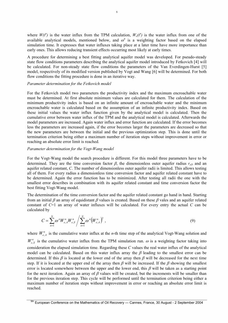
Figure 1: Aquifer and productive area grid connected via an artificial boundary (shaded) used for history run of Example 1.

Figure 2: Pressure declines for Example 1

Figure 3: Aquifer grid that results from the parameter conversion of Example 1.

Figure 4: Pressure declines for Example 1

2

Figure 5: Heavily faulted productive area grid with artificial boundary (shaded) of Example 2.

Figure 7: Heavily faulted productive area grid of Example 3. Artificial boundary and related target area are shaded with the same color.

Figure 9: Aquifer grid resulting from the conversion of analytical to gridded parameters for Example 3.

Figure 6: Pressure declines for Example 2.

Figure 8: Pressure decline for the target area located in the West of Example 3.

Figure 10: Pressure decline for the target area located in the West of Example

3

9th European Conference on the Mathematics of Oil Recovery — Cannes, France, 30 August - 2 September 2004