IEEE TRANSACTIONS ON INSTRUMENTATION AND MEASUREMENT, VOL. 54, NO. 4, AUGUST 2005 1463

Automatic Multiscale MeshingThrough HRBF Networks

Stefano Ferrari, Iuri Frosio, Vincenzo Piuri, Fellow, IEEE, and N. Alberto Borghese, Member, IEEE

Abstract—A procedure for the real-time construction of three-dimensional (3-D) multiscale meshes from not evenly sampled 3-Dpoints is described and discussed in this paper. The process is basedon the connectionist model named hierarchical radial basis func-tions network (HRBF), which has been proved effective in the re-construction of smooth surfaces from sparse noisy data points. Thenetwork goal is to achieve a uniform reconstruction error, equal tomeasurement error, by stacking noncomplete grids of Gaussians atdecreasing scales. It is shown here how the HRBF properties canbe used to develop a configuration algorithm, which produces acontinuous surface in real time. In addition, the model is extendedto automatically convert the continuous surface into a 3-D meshaccording to an adequate error measure.

Index Terms—Adaptive meshing, cloud of points, multiscalesurface, noise filtering, real-time meshing, three-dimensional (3-D)scanner.

I. INTRODUCTION

THREE-DIMENSIONAL (3-D) scanning of real objectsis becoming a common technique to obtain 3-D models.

The procedure is composed of two-steps: 1) measuring a set of(not evenly sampled) data points on the object’s surface (cloudof points, cf. Fig. 1) and 2) generating a 3-D colored mesh,which is the de-facto standard in 3-D visualization. Althoughsampling can be indeed fast, the generation of a 3-D meshrequires a considerable amount of time as the processing chainusually requires combining a set of partial 3-D scans (each takenwith a different location and attitude of the sensors) to producea complex 3-D model. This is achieved by looping throughthree steps: view planning, scans alignment (registration), andsurface reconstruction through merging [1]. Each partial scancan be constituted of several hundreds of thousands of datapoints and represents a portion of the scanned object. Toacquire the entire object human intervention is required toplan additional scans, which would add to the model missingdetails or the object’s portions not acquired in the previousscans. As a consequence of this evaluation planning procedure,the acquisition of a single model can take a very long time.

Manuscript received June 15, 2004; revised April 4, 2005. The research wassupported in part by the Italian Ministry of Education, University of Research(MIUR) under Grant 449/97, “RoboCare: A MultiAgent System with Intelligentand Mobile Robotic Components.”

S. Ferrari and V. Piuri are with the Department of Information Technolo-gies, University of Milano, 26013 Crema, Italy (e-mail: ferrari@dti.unimi.it;piuri@dti.unimi.it).

I. Frosio and N. A. Borghese are with the Department of Computer Sci-ence, University of Milano, 20135 Milan, Italy (e-mail: frosio@dsi.unimi.it;borghese@dsi.unimi.it).

Digital Object Identifier 10.1109/TIM.2005.851471

Fig. 1. Doll face in panel (a) has been scanned through the Autoscan digitizer[7], obtaining a data set of 16 851 range data points reported in panel (b).

The process can be speeded up, if a visual feedback is madeavailable in real time. In this case, subsequent scans can be effi-ciently planned within a short time. A solution in this directionhas been recently proposed by [2], where a simplified renderingof the surface was introduced to evaluate image quality. In thistechnique, called splatting, an oriented planar circular shape isrendered around each sampled point to convey an idea of thesurface geometry.

The approach presented here is aimed at obtaining in real-timemultiscale meshes of high quality. It is based on the hierarchicalradial basis function networks model (HRBF) [3], [4]), wherea linear combination of Gaussian units is adopted to representthe surface. The HRBF model was derived in the connectionistdomain, where the problem of fitting a mesh to range data isstudied into the broad domain of multivariate approximation [5].The main characteristic of the model is the ability to reconstructa 3-D surface with no iteration on the data, therefore allowingfast computation of the configuration parameters. The closestapproach to HRBF is based on stacking grids of B-splines[6]. In the HRBF configuration algorithm, the parameters arecomputed through algebraic operations carried out locally onthe data: the computation of each HRBF’s parameter requiresconsidering only a subset of the data. To add finer details ofthe surface, which are often circumscribed in a few regions, amultiscale adaptive scheme has been developed. This schemaautomatically identifies these regions and inserts clusters ofGaussians at smaller scales there. This local nature of thecomputation can be exploited to obtain a real-time procedurefor network configuration. Besides this, it is also shown howthe differential properties of the Gaussian units allow defining

0018-9456/$20.00 © 2005 IEEE

1464 IEEE TRANSACTIONS ON INSTRUMENTATION AND MEASUREMENT, VOL. 54, NO. 4, AUGUST 2005

a particular error measure, which can be used to guide theadaptive resampling of the continuous HRBF surface to obtainthe 3-D mesh.

The paper is organized as follows. The HRBF model is brieflysummarized in Section II. In Section III, the procedure to obtainreal-time surface computation is described, and in Section IV,it is shown how to sample the surface to obtain a 3-D mesh.Results are reported in Section V and a few concluding remarksin Section VI.

II. HRBF MODEL

Let us suppose that the measured points can be expressedas a two-dimensional (2-D) data set, that is, as a height field

. In thiscase, the surface will assume the explicit analytical shape

. The output of the HRBF network is obtained by addingthe output of a stack of hierarchical layers , at decreasingscales, as follows:

(1)

where determines the scale of the th layer, with. When the Gaussian is

taken as basis function, the output of each layer can be writtenas

(2)

where is the number of Gaussian units of the th layer. Theare equally spaced on a 2-D grid, which covers the input

domain of the range data, that is, the ’s are positioned inthe grid crossings. The side of the grid is a function of the scaleof that layer: the smaller the scale, the shorter is the side length,the denser are the Gaussians, and the finer are the details thatcan be reconstructed.

The shape of the surface in (2) depends on a set of parameters:the structural parameters, which are the number ,the scale ensemble , the position , and the weights as-sociated to each Gaussian . Each grid realizes a low-passfilter, which is able to interpolate and reconstruct the surface upto a certain scale, determined by . Considerations, groundedon the signal processing theory, allow, given a certain scale ,to set the grid side and, consequently, and the [8].In this schema, the weights represent the surface heightmeasured in the grid crossings . As measuredpoints are usually not equally spaced, is not availableand should be estimated. To that purpose, a weighted average ofthe measured points , where the weight decreases with thedistance of from , can be adopted. The estimate can becarried out locally in space, by using only those points lying inan appropriate neighborhood of . This neighborhood, calledreceptive field , can be chosen as a circular region cen-

Fig. 2. Surfaces of the doll face in Fig. 1 obtained by multilayer HRBFreconstruction. The surfaces in (a)–(d) are obtained from the fast HRBFalgorithm by using one to four layers; the ones in (e)–(h) are obtained fromthe fast meshing algorithm by restricting the meshing on the centers of,respectively, the first up to the fourth layer; the surfaces in (i)–(n) are generatedby the fast meshing algorithm, with different threshold � (0.5, 0.1, 0.05, 0.01,respectively). The surfaces in (a)–(d) are obtained by densely resampling theHRBF surface (61161 triangles). The meshes in (e)–(h) are composed by 1276,4321, 12578, and 28 296 triangles, respectively. The surfaces in (i)–(n) arecomposed by 8094, 28296, 39797, and 63 172 triangles, respectively.

tered in , which have the radius proportional to the grid side. A possible weighting function is

(3)

Although a single layer with Gaussians of very small scalecan reconstruct the finest details, this would produce an unnec-essary dense packing of units in all those regions that ure a low

FERRARI et al.: AUTOMATIC MULTISCALE MESHING THROUGH HRBF NETWORKS 1465

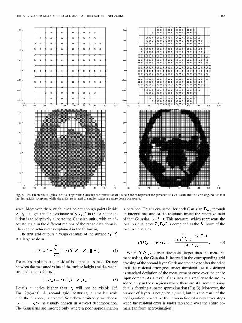
Fig. 3. Four hierarchical grids used to support the Gaussian reconstruction of a face. Circles represent the presence of a Gaussian unit in a crossing. Notice thatthe first grid is complete, while the grids associated to smaller scales are more dense but sparse.

scale. Moreover, there might even be not enough points insideto get a reliable estimate of in (3). A better so-

lution is to adaptively allocate the Gaussian units, with an ad-equate scale in the different regions of the range data domain.This can be achieved as explained in the following.

The first grid outputs a rough estimate of the surfaceat a large scale as

(4)

For each sampled point, a residual is computed as the differencebetween the measured value of the surface height and the recon-structed one, as follows:

(5)

Details at scales higher than will not be visible [cf.Fig. 2(a)–(d)]. A second grid, featuring a smaller scalethan the first one, is created. Somehow arbitrarily we choose

, as usually chosen in wavelet decomposition.The Gaussians are inserted only where a poor approximation

is obtained. This is evaluated, for each Gaussian , throughan integral measure of the residuals inside the receptive fieldof that Gaussian . This measure, which represents thelocal residual error is computed as the norm of thelocal residuals as

(6)

When is over threshold (larger than the measure-ment noise), the Gaussian is inserted in the corresponding gridcrossing of the second layer. Grids are created one after the otheruntil the residual error goes under threshold, usually definedas standard deviation of the measurement error over the entireinput domain. As a result, Gaussians at a smaller scale are in-serted only in those regions where there are still some missingdetails, forming a sparse approximation (Fig. 3). Moreover, thenumber of layers is not given a priori, but it is the result of theconfiguration procedure: the introduction of a new layer stopswhen the residual error is under threshold over the entire do-main (uniform approximation).

1466 IEEE TRANSACTIONS ON INSTRUMENTATION AND MEASUREMENT, VOL. 54, NO. 4, AUGUST 2005

III. FAST CONFIGURATION OF HRBF SURFACES

For each layer , the complexity of the configuration algo-rithm is , where is the number of the Gaussians ofthe network, and is the data set cardinality. This figure re-sults by observing that the computation of both the residuals andthe coefficients requires evaluating the distancebetween each measured point and the position of eachGaussian ((3) and (6)). The need to compute the distancebetween all data points and all Gaussian centers is required by1) the nonzero response of the Gaussian in the whole domain

(infinite support) and 2) the extraction of the points that lieinside the receptive field.

To reduce the configuration time, several observations can bemade. As Gaussian decreases rapidly toward zero, in practicalapplications, its influence is considered only inside a suitableneighborhood of the Gaussian center, which will be termedinfluence region. In the following, will be taken as radius of

, where is times the value of the value ofthe Gaussian in its center.

To avoid the need of computing, for each unit (the distancefrom all the measured points), the key idea is to arrange the datain a data structure that allows fast retrieval of those points, whichbelong to the neighborhood of a unit. Easy partitioning cannotbe obtained with the circular regions implicitly considered inthe definition of and ; some approximations must beintroduced, in particular, the following.

1) The receptive field of the Gaussians is approximated bythe bounding square. From now on, we simply refer tothese squared boxes as the receptive field.

2) The length of the side of the receptive field is an evenmultiple of the grid spacing . More formally, the re-ceptive field side is equal to , where .

3) The Gaussian width (and, hence, the grid side ) ishalved at every layer, as follows: .

The influence region will also be represented as a squared regionof side multiple of the Gaussian spacing.

To take full advantage of locality, a quad-tree-like datastorage mechanism, which organizes the data points using arecursive splitting of the input domain along both the axes andallows a fast retrieval of closed points, has been introduced[9]. Let us suppose that measured data points are stored intoan array: they will be arranged such that their position in thearray will reflect their position in 3-D space. In particular,points that lie inside the same influence region will be stored inclose positions of the data array. To the scope, we introduce theconcept of a cell, called , as the squared region on the supportplane , whose vertexes are four adjacent Gaussian centers(cf. Fig. 3). Since it assumes the value of the grid side , thesize of the side of a cell changes from layer to layer. To each

, a data structure is associated, which contains the number ofdata points projecting over , , and the position in the arraywhere the first point lying inside is stored . All the points,which lie inside a cell , can be retrieved easily from and

. This arrangement of the data guarantees the following:

• receptive field and influence region direct mapping (theindexes of the cells associated to each Gaussian, can bedirectly computed from the Gaussian position index);

Fig. 4. Implementation of the partitioning schema into cells.

• quad-tree data partitioning (the cell of a higher layercan be generated by efficiently partitioning the corre-sponding cells of the lower layer: the union of four cellsof the higher layer produces a single cell of the imme-diate lower layer).

The rearrangement of the points is obtained by an in-place par-tial sorting algorithm, a variant of Quicksort, in which the pivotvalue is the mean position of the data inside the vector segmentassociated to the each cell [10]. The partitioning schema is il-lustrated in Fig. 4, and it can be efficiently used to compute theparameters in (3) and (6).

This processing greatly improves the configuration procedureperformances, as each point is now involved in the computa-tion of no more than Gaussians for each layer. Hence,the computational time linearly scales with the cardinality ofthe data set . For example, the reconstruction of the surfacereported in Fig. 2(a)–(d) required a processing time of 1.78 s(with a standard deviation of 0.118 s) averaged over 20 trials,on a Pentium III 1-GHz machine with 256 MB of memory. TheHRBF data are reported in Table II. The amount of overheadadded by data structuring was negligible, being of one order ofmagnitude smaller than network configuration time.

IV. FROM HRBF SURFACES TO HRBF MESHES

The output of the HRBF network is a multiscale continuoussurface. To be visualized by graphical hardware, this surface hasto be digitized, that is converted into a multiscale mesh. This is apiecewise planar approximation of the surface. One possibilityis to densely sample the surface and tessellate it. However, thiswould produce an unnecessary dense mesh.

A better solution can be obtained by exploiting the differentialproperties of the HRBF surface, to produce a mesh such that thevertices are denser in those regions containing the finest details.The rationale is to start with a low-density mesh and to makeit denser around the points , in which the deviation fromlinearity is greater than a given threshold . Let us call Errthis deviation and define it as

Err polyg (7)

If the evaluation of Err were carried out by computingas in (1), there would be no advantage in later discarding

the point from the mesh (at least in terms of meshing accuracy,computational time, and memory allocation). However, the dif-ferential properties of the HRBF model grant us a cheap esti-mate of the surface height: as shown in the Appendix , since thederivatives of each Gaussian can be computed mostly reusingsome of the intermediate results of the network configuration

FERRARI et al.: AUTOMATIC MULTISCALE MESHING THROUGH HRBF NETWORKS 1467

Fig. 5. HRBF fast meshing schema. In panel (a), the base points are shown.In panel (b), the set of probing points P is shlown in light gray. The value inP is estimated starting from the HRBF value computed in U . In panel (c), anexample of residual evaluation computed for each P is shown. The points withthe dark outer circle are over threshold and lead to the addition of new vertexesas shown in panel (d).

procedure, the computation of the derivatives of the HRBF sur-face is very efficient. This fact can be fully exploited when usinga second-order approximation of the HRBF surface in (7)instead of the HRBF value , given by (1).

The meshing procedure starts by considering the crossings ofthe first grid , which we call base points[cf. Fig. 5(a)]. The HRBF surface is sampled in to obtain

, which constitutes a first ensemble of mesh vertexes.Notice that the surface height in the base points is obtained assum of the outputs of all the layers (1) [e.g.,Fig. 2(a)].

The adequacy of the resulting mesh is evaluated by analyzingthe approximation error between pairs of adjacent base points:we will make the mesh denser (of vertices), where the approxi-mation error is higher. To the scope, a probing set is chosenas the set of the midpoints of the segments connecting two adja-cent base points. It should be noted that is a subset of thecrossings of the second grid.

The height of the reconstructed surface in each probing point, is estimated through the second-order Taylor expansion of

the HRBF , evaluated in the neighboring grid cross-ings of , . In particular, is evaluated asthe average of the surface height estimated in the points whichbelong to through , as follows:

(8)

Fig. 5(b) depicts these operations. The arrows depart from anelements of and reach a probing point the neighborhood towhich they belong. For each probing point, the estimated heightis computed according to (8) and it is compared with the piece-wise approximation in , , of-fered by the mesh. The probing point is added to the meshonly if, for a given threshold , the condition

(9)

holds. Hence, the difference is used to estimatethe distance between the HRBF surface and its polygonal ap-proximation in the point . If this distance is higher of a giventhreshold , the point is added to the base points set, andits HRBF surface height is computed [Fig. 5(c) and (d)]. Thisschema is iterated until a given criterion is met.

For example, the meshes in Fig. 2(e)–(h) and the meshes inFig. 2(i)–(n) are computed using this schema but different stop-ping criteria. For the meshes of the first group, we restrict the

TABLE IRECONSTRUCTION PERFORMANCE OF THE ORIGINAL HRBF

TABLE IIRECONSTRUCTION PERFORMANCE OF THE FAST HRBF

TABLE IIIRECONSTRUCTION PERFORMANCE OF THE FAST MESHING

meshing on the center of the different layers [the first up to theforth layer for the meshes in Fig. 2(e)–(h), respectively]. Hence,the stopping criterion is the number of iterations of the meshingprocedure. Instead, the meshes in Fig. 2(i)–(n) have been con-structed iterating the previously described procedure until thesurface results under threshold in all the probing points.

V. ACCURACY

To implement and use the HRBF processing, the underlyingtheoretical foundations need to be relaxed by introducing suitedapproximation addressing feasibility and performance issues.

In the processing chain previously described, approximationsare induced in both the residual computation and the resam-pling stages. In the computation of the residual stage, approx-imations are introduced by arbitrarily limiting the contributionof a Gaussian inside a square region that surround the Gaussianitself, while in the meshing stage the choice of an estimatorfor predicting the surface height may result in a mesh of poorquality.

In order to monitor the accuracy in the HRBF processingchain, we compare the reconstruction obtained in each stagewith respect to the original data set. To evaluate accuracy weadopt the root mean square error (RMSE) and the mean andstandard deviation of the absolute value of the reconstructionerror ( and ).

Tables I–III report the figures of merit for the reconstructionobtained from the original HRBF algorithm (Gaussians with in-finite support), the HRBF trained with the fast schema (Gaussianwith bounded support), and the fast meshing schema (predictor

1468 IEEE TRANSACTIONS ON INSTRUMENTATION AND MEASUREMENT, VOL. 54, NO. 4, AUGUST 2005

TABLE IVACCURACY PERFORMANCE COMPARISON

TABLE VACCURACY PERFORMANCE COMPARISON OF GENERATED MESHES

guided meshing with ). These figures of merit of the firstand the second reconstruction compare well with the measure-ment error of the data (0.7 mm). In Table III, instead of reportingthe structural parameters of the HRBF network (which are thesame of the network in Table II), the number of vertices and tri-angles of the resulting meshes are reported.

Table IV reports the accuracy figures of the fourth level ofthe reconstruction algorithm (original and fast HRBF) com-pared with the ones achieved by the fast meshing over severalvalues of the threshold . The generated surfaces are reportedin Fig. 2(i)–(n).

Table V reports the figures of merit achieved by the fastmeshing computed with respect to the approximation of theoriginal data given by the mesh obtained from the resamplingof the fast HRBF algorithm. Besides, it reports the number ofvertices and triangles of the generated meshes.

VI. DISCUSSION AND CONCLUSION

As shown in Tables I–III, the accuracy is not affected by theapproximation introduced by the implementation choices. Ex-periments operated on several data sets confirm this conclusion.

In the computation of the residual stage (6), in order to savecomputational time, we arbitrarily limit the contribution of aGaussian inside a square centered in the Gaussian center. Thischoice is acceptable in spaces of low dimensionality as in ourcase. When increases, the volume of a -dimensional spherebecomes negligible with respect to the volume of its bounding

-dimensional cube, and the choice is not justified anymore.Spherical neighborhood region computation requires additionalprocessing, which makes this approach less appealing. How-ever, the accuracy of the reconstruction is not affected as thecontribution of a Gaussian is negligible outside its neighbor-hood region. Moreover, it is worth noting that the approxima-tion error of a layer can be recovered by the next layer, sincethis is included in the residual [4], [11].

Another potential source of inaccuracies is the use of an es-timator in (8) to decide if the mesh resampling should be moredense. As vertices added to the mesh depend on the surface pre-diction (8), inaccuracy of the prediction may result either in amesh unnecessarily dense or in a mesh poor of details.

As pointed out by the figures of merit reported in Table IV,the use of the second-order Taylor expansion as surface pre-dictor has proven to be effective. However, the comparison (9)between the height of predicted surface and the height of thepolygonal approximation in itself may not be adequate in mea-suring the difference of the visual appearance of the two sur-faces. Fig. 2(i)–(n) illustrates this point, as they are generatedby using only the threshold as stopping criterion to drive themeshing procedure. Comparing them with the surfaces reportedin Fig. 2(e)–(h), it is evident that they employ an unneccessarilyhigh number of triangles to reconstruct the surface, whether astopping criterion based on the number of vertices may balancethe opposite requirements of accuracy and lightness of the mesh.For the task of measuring the difference in visual appearance, abetter figure of merit could be the distance between the polyg-onal approximation and its projection onto the predicted surface.However, this operation cannot be used in the present applica-tion due to its high computational cost.

The relaxation of some theoretical aspects of the hierarchicalradial basis functions (HRBF) algorithm allows implementingan efficient computation of the HRBF parameters, whichoperate locally on the data and achieve real-time meshing onsequential machines. Computing time overhead for the prepro-cessing is negligible, being experimentally measured of oneorder of magnitude smaller than configuration time.

Errors that might be introduced by the implementationchoices (e.g., the quantization error [11], the approximationsintroduced in Section III) do not decrease the reconstructionaccuracy, because of the constructive nature of the configura-tion algorithm. The figures of merit of the reconstruction errorfor traditional and the fast configuration algorithms are in factalmost identical, as shown in Tables I and II. A comparisonbetween the two reconstructed surfaces is shown in Fig. 6. Itcan be noticed that in the region covered by the points, thedifference is almost negligible.

The fast meshing schema allows achieving real-timemeshing, at least for a preview of the reconstruction, whichallows real-time assessment of the quality of the obtainedmodel. As reported in Fig. 7, the error is distributed mainly inthe border region, while it is perceptually negligible in the innerregion. It should be noted that as most of the expansions arecomputed along the axis, they do not require all the derivatives.In other words, once the HRBF surface has been com-puted, with little additional effort, the function , whichevaluates the surface height with respect to , is available. Theaccuracy of the generated mesh allows correcting the scanningsetup and planning additional refinement scans immediately inorder to avoid artifacts or holes in the produced mesh.

Moreover, the accuracy achieved by the fast meshing schemais adjustable by the threshold . The value can be regulatedon both the computational resources, which can be devoted tothe meshing procedure, and the capability of the visualizationdevice. Besides, the generated mesh can be a good starting point

FERRARI et al.: AUTOMATIC MULTISCALE MESHING THROUGH HRBF NETWORKS 1469

Fig. 6. Reconstruction error of the fast configuration schema.

Fig. 7. Reconstruction error of the fast meshing schema.

for mesh optimization procedures, since it can be enriched withinformation on the differential properties of the surface. Thisinformation may be obtained with a little additional effort bythe resampling procedure.

APPENDIX

The second-order Taylor’s expansion of a functionis

(10)

where and and are the components of along theaxes.

Reframing (1) as

(11)

the derivatives of the HRBF surface (1) can be computed as

(12)where and , and

(13)

(14)

(15)

(16)

REFERENCES

[1] M. Levoy, K. Pulli, B. Curless, S. Rusinkiewicz, D. Koller, L. Pereira, M.Ginzton, S. Anderson, J. Davis, J. Ginsberg, J. Shade, and D. Fulk, “Thedigital Michelangelo project: 3-D scanning of large statues,” in Proc.Computer Graphics (Siggraph 2000) (Annual Conf. Series), K. Akeley,Ed., Jul. 2000, pp. 131–144.

[2] S. Rusinkiewicz, O. Hall-Holt, and M. Levoy, “Real-time 3-D modelacquisition,” in Proc. 29th Annu. Conf. Computer Graphics InteractiveTechniques, San Antonio, TX, 2002, pp. 438–446.

[3] N. A. Borghese and S. Ferrari, “A portable modular system for automaticacquisition of 3-D objects,” IEEE Trans. Instrum. Meas., vol. 49, no. 5,pp. 1128–1136, Oct. 2000.

[4] S. Ferrari, M. Maggioni, and N. A. Borghese, “Multi-scale approxi-mation with hierarchical radial basis functions networks,” IEEE Trans.Neural Netw., vol. 15, no. 1, pp. 178–188, Jan. 2004.

[5] F. Girosi, M. Jones, and T. Poggio, “Regularization theory and neuralnetworks architectures,” Neural Comput., vol. 7, no. 2, pp. 219–269,1995.

[6] S. Lee, G. Wolberg, and S. Y. Shin, “Scattered data interpolation withmultilevel B-splines,” IEEE Trans. Vis. Comput. Graphics, vol. 3, no. 3,pp. 228–244, Jul. 1997.

[7] N. A. Borghese, G. Ferrigno, G. Baroni, R. Savarè, S. Ferrari, and A.Pedotti, “Autoscan: A flexible and portable scanner of 3-D surfaces,”IEEE Comput. Graph. Appl., vol. 18, no. 3, pp. 38–41, May–Jun. 1998.

[8] N. A. Borghese and S. Ferrari, “Hierarchical RBF networks and localparameter estimate,” Neurocomputing, vol. 19, no. 1–3, pp. 259–283,1998.

[9] N. A. Borghese, S. Ferrari, and V. Piuri, “Real-time surface reconstruc-tion through HRBF networks,” in Proc. IEEE Int. Workshop HapticVirtual Environments Their Applications (HAVE 2002), Nov. 2002, pp.19–24.

[10] C. A. R. Hoare, “Algorithms 64: Quicksort,” Commun. ACM, vol. 4, no.7, p. 321, 1961.

[11] S. Ferrari, N. A. Borghese, and V. Piuri, “Multiscale models for dataprocessing: An experimental sensitivity analysis,” IEEE Trans. Instrum.Meas., vol. 50, no. 4, pp. 995–1002, Aug. 2001.

Stefano Ferrari received the computer science degree from the University ofMilano, Italy, in 1995 and the Ph.D. degree in computer and automation engi-neering from the Politecnico di Milano, Milan, Italy, in 2001.

Since 2003, he has been an Assistant Professor with the Department of Infor-mation Technologies, University of Milano, Crema, Italy.

His research interests are related mainly to neural networks and soft-com-puting paradigms and their application to the computer graphics.

1470 IEEE TRANSACTIONS ON INSTRUMENTATION AND MEASUREMENT, VOL. 54, NO. 4, AUGUST 2005

Iuri Frosio is currently working toward the Ph.D. degree at the BioengineeringDepartment of Politecnico of Milan.

He is currently with the Information Science Department, University ofMilano, Milan, Italy, where he works as a Research Fellow at the AppliedIntelligent Systems (AIS) Laboratory. His research interests include three-dimensional reconstruction, motion capture systems, neural networks, digitalradiography, and tomography.

Vincenzo Piuri (S’84–M’86–SM’96–F’01) received the Ph.D. degree in com-puter engineering from the Politecnico di Milano, Crema, Italy, in 1989.

From 1992 to September 2000, he was an Associate Professor of OperatingSystems at the Politecnico di Milano. Since October 2000, he has been aFull Professor of Computer Engineering at the University of Milano, Milan,Italy. He was a Visiting Professor at the University of Texas at Austinduring summers 1993 and 1999. His research interests include distributedand parallel computing systems; computer arithmetic; application-specificprocessing architectures; digital signal processing architectures; fault tolerance;neural network architectures; theory and industrial applications of neuraltechniques for identification, prediction, and control; and signal and imageprocessing. His original results have been published in more than 150 papersin book chapters, international journals, and proceedings of internationalconferences.

Prof. Piuri is a Member of Association for Computing Machinery (ACM),the International Neural Network Society, and the Italian Electrotechnical andElectronic Association (AEI). He is Vice-President for Publications of theIEEE Instrumentation and Measurement Society, Vice-President for MemberActivities of the IEEE Neural Networks Society, and a Member of the Ad-ministrative Committees of both the IEEE Instrumentation and MeasurementSociety and the IEEE Neural Networks Society. He is an Associate Editor ofthe IEEE TRANSACTIONS ON NEURAL NETWORKS and the Journal of SystemsArchitecture.

N. Alberto Borghese (M’97) graduated with full honors in electrical engi-neering from the Politecnico of Milano, Milan, Italy in 1985.

He is Associate Professor at the Department of Computer Science of theUniversity of Milano, Milan, Italy, where he teaches Intelligent Systemsand Digital Animation and directs the Laboratory of Applied IntelligentSystems. He was Visiting Scholar at the Center for Neural Engineering ofthe University of Southern California (USC), Los Angeles, in 1991, at theDepartment of Electrical Engineering of the California Institute of Technology(Caltech), Pasadena, in 1992, and at the Department of Motion Capture ofElectronic Arts, Vancouver, Canada, in 2000. His research interests includequantitative human motion analysis, modeling and synthesis in virtual reality,and artificial learning systems, areas in which he has authored more than30 refereed journal papers.