The Multiscale Approach to

Error Estimation and Adaptivity

Guillermo Hauke a,∗, Mohamed H. Doweidar a, Mario Miana b

aDepartamento de Mecanica de Fluidos, Centro Politecnico Superior,C/Maria de Luna 3, 50018 Zaragoza, Spain

bArea de Mecanica y Nuevos Materiales, Instituto Tecnologico de Aragon,C/Maria de Luna 7, 50018 Zaragoza, Spain

Abstract

A new explicit a posteriori error estimator is investigated, which emanates fromthe variational multiscale theory. The error estimator uses an approximation of theGreen’s function which propagates the error according to the dual problem. Thetechnique predicts the error in the L2 norm from element residuals, both interiorand inter-element jumps, therefore, leading to a very economical procedure. Finally,the methodology is applied to fluid flow transport, showing that for convection-dominated flows, the efficiency index is independent of the diffusion coefficient.

Key words: a posteriori error estimation, advection-diffusion-reaction equation,stabilized methods, variational multiscale methodPACS: 47.11.+j

1 Introduction

Nowadays, computational mechanics has achieved a great degree of maturity,shown by the robustness level of present solvers. Therefore, the challenge inthis field is shifting from just computing a solution, towards attaining a reliable

solution with the desired of accuracy.

In order to attain reliable solutions, in the past the stress has been typicallyplaced on the user and his/her experience. For simple solutions this might be

∗ Corresponding author.Email address: ghauke@unizar.es (Guillermo Hauke).

Preprint submitted to Elsevier Science 18 February 2005

adequate, but gross mistakes in important engineering problems alerted thatthis is not the right strategy, mainly in problems with boundary and internallayers, which are present in both, fluid and solid mechanics. Therefore, latelyexperience is being replaced by mathematical techniques to predict and controlthe numerical error.

Furthermore, computer power is not unlimited, but scarce, mainly in three-dimensional applications. Even the human and economical resources of a com-pany or institution are also limited and should be used wisely. So mathematicalerror control not only can increase the accuracy of the solution, but also canoptimize both, computer and human resources.

The quote ”If you have the mesh, you have the solution,” reflects very wellthe state of the art [22] and the points above risen. In order to have a goodsolution, one needs the right mesh, which depends on the solution.

Therefore, this paper is about obtaining the right mesh, which means obtainingreliable solutions in acceptable times, and optimizing the computer and humanresources.

The error control strategy, then, is typically found following these steps.

(1) Developing a reliable error prediction tool.(2) Controlling the error by selecting the element size or the polynomial

degree.(3) Adapting the mesh.

The final goal that it is proposed here goes a little bit further: to attain asolution with a user-prescribed accuracy, without the user interaction.

Pioneering work on error estimation was developed for elliptic problems byBabuska and Rheinbolt [6], was followed by Zienkiewicz and Zhu [45,46],Eriksson and Johnson [15], Ainsworth and Oden [2], among others. Stew-art and Hughes also made contributions in [38,39]. The above ideas were thenapplied to hyperbolic and fluid mechanics problems, for instance by Oden etal. [32,33], Johnson and coworkers [28–30], Strouboulis and Oden [40], andVerfurth [43]. Developing strict bounds for linear-functionals of the solution isanother promising approach to error control (see [36]). For a more elaboratereview, the reader can consult [3,4].

According to [4], present methods for a posteriori error estimation can beclassified as follows.

(1) Residual-based methods, when they compute residuals, both, interior and/orinter-element or boundary residuals. Typically, they use directly the ap-proximate finite element solution, and so, are called explicit methods.

2

Explicit residual-based error estimators were proposed for the first timeby Babuska and Rheinbolt [9], and then extended to two-dimensionsin [5,31].

(2) Recovery-based methods. These techniques employ superconvergent prop-erties of the solutions and were first proposed by [45,46]. They can beused at the element level or using patches of elements [47,48]. A generalframework for the analysis of the above methods can be found in [1]. Forapplications to aerodynamics see [44,13] and for a recent contribution,[34].

(3) Auxiliary-problem-based methods. In this technique, new partial differen-tial equations are solved either at the element level, in subdomains orin the whole domain. Since estimating the error requires solving a newproblem, they are also called implicit error estimators. Pioneering workwas started by [6–8,10]. Recent contributions are those in [26,14,21], forinstance.

Recent works, such as [27,35], review and compare the performance of themost successful a posteriori error estimators when applied to fluid mechan-ics problems. Their conclusions are not optimistic, since all authors concludethat for fluid transport, present techniques are far from satisfactory. Simplealgorithms are non robust, that is, the ratio of predicted to true error changesdramatically with the diffusion coefficient. Some solutions exists but requiresolving additional partial differential equations, which can turn computation-ally expensive.

Thus, in this paper we investigate the application of the variational multiscaleapproach [24] to the development of explicit a posteriori error estimators ingeneral, and to fluid transport problems in particular.

2 Basic concepts of a posteriori error estimation

To assess the quality of an a posteriori error estimator, the academic conceptof efficiency or effectivity index Ieff is introduced. It is defined as the ratio ofa norm of the predicted error, to the norm of the true error,

Ieff =|||Predicted error|||

|||True error||| (1)

where ||| · ||| is an appropriate norm. If u is the exact solution, uh the finiteelement solution, and η the error indicator, then

Ieff =η

|||uh − u||| (2)

3

Desirable properties of a good a posteriori error estimator are [42,27]:

• Efficiency: if Ieff and I−1eff are bounded for all triangulations.

• Robustness: if Ieff and I−1eff are bounded independently of the problem.

Robustness implies, therefore:

• The efficiency index is approximately one (Ieff ≈ 1) independently of pa-rameters (in particular, the diffusivity coefficient), boundary conditions andmesh size.

• Ieff converges uniformly at the same rate as the actual error, that is, givenCl and Cr positive constants,

Cl|||True error||| ≤ |||Predicted error||| ≤ Cr|||True error||| (3)

or

Cl|||uh − u||| ≤ η ≤ Cr|||uh − u||| (4)

The difference between efficiency and robustness resides in the the type ofconvergence. Robustness implies more quality than efficiency since requiresuniform convergence.

3 The variational multiscale approach to error estimation

3.1 The abstract problem

Consider a spatial domain Ω with boundary Γ, which is partitioned into twonon-overlapping zones Γg and Γh. The strong form of the boundary-value prob-lem consists of finding u : Ω → R such that for the given essential boundarycondition g : Γg → R, the natural boundary condition h : Γh → R, and forcingfunction f : Ω → R, the following equations are satisfied

Lu = f in Ω

u = g on Γg

Bu = h on Γh

(5)

where L is in principle a second-order differential operator and B an operatordefined later, acting on the boundary.

Given the functional solution space S ⊂ H1(Ω) and weighting space V ⊂H1(Ω), with H1(Ω) the Sobolev space of order one, the variational formulation

4

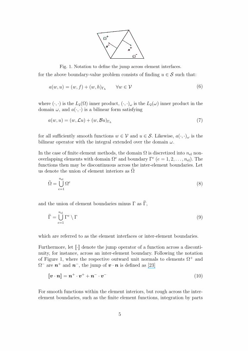
Fig. 1. Notation to define the jump across element interfaces.

for the above boundary-value problem consists of finding u ∈ S such that:

a(w, u) = (w, f) + (w, h)Γh∀w ∈ V (6)

where (·, ·) is the L2(Ω) inner product, (·, ·)ω is the L2(ω) inner product in thedomain ω, and a(·, ·) is a bilinear form satisfying

a(w, u) = (w,Lu) + (w,Bu)Γh(7)

for all sufficiently smooth functions w ∈ V and u ∈ S. Likewise, a(·, ·)ω is thebilinear operator with the integral extended over the domain ω.

In the case of finite element methods, the domain Ω is discretized into nel non-overlapping elements with domain Ωe and boundary Γe (e = 1, 2, . . . , nel). Thefunctions then may be discontinuous across the inter-element boundaries. Letus denote the union of element interiors as Ω

Ω =nel⋃

e=1

Ωe (8)

and the union of element boundaries minus Γ as Γ,

Γ =nel⋃

e=1

Γe \ Γ (9)

which are referred to as the element interfaces or inter-element boundaries.

Furthermore, let [[·]] denote the jump operator of a function across a disconti-nuity, for instance, across an inter-element boundary. Following the notationof Figure 1, where the respective outward unit normals to elements Ω+ andΩ− are n

+ and n−, the jump of v · n is defined as [23]

[[v · n]] = n+ · v+ + n

− · v− (10)

For smooth functions within the element interiors, but rough across the inter-element boundaries, such as the finite element functions, integration by parts

5

leads to

a(w, u)=nel∑

e=1

a(w, u)Ωe

=nel∑

e=1

((w,Lu)Ωe + (w,Bu)Γe

)

= (w,Lu)Ω

+ (w, [[Bu]])Γ

+ (w,Bu)Γh(11)

where B is the corresponding boundary operator emanating from integrationby parts.

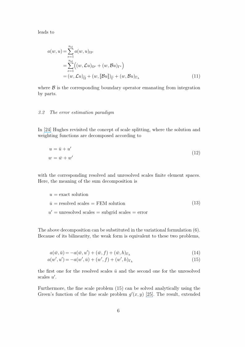
3.2 The error estimation paradigm

In [24] Hughes revisited the concept of scale splitting, where the solution andweighting functions are decomposed according to

u = u + u′

w = w + w′

(12)

with the corresponding resolved and unresolved scales finite element spaces.Here, the meaning of the sum decomposition is

u = exact solution

u = resolved scales = FEM solution

u′ = unresolved scales = subgrid scales = error

(13)

The above decomposition can be substituted in the variational formulation (6).Because of its bilinearity, the weak form is equivalent to these two problems,

a(w, u)=−a(w, u′) + (w, f) + (w, h)Γh(14)

a(w′, u′)=−a(w′, u) + (w′, f) + (w′, h)Γh(15)

the first one for the resolved scales u and the second one for the unresolvedscales u′.

Furthermore, the fine scale problem (15) can be solved analytically using theGreen’s function of the fine scale problem g′(x, y) [25]. The result, extended

6

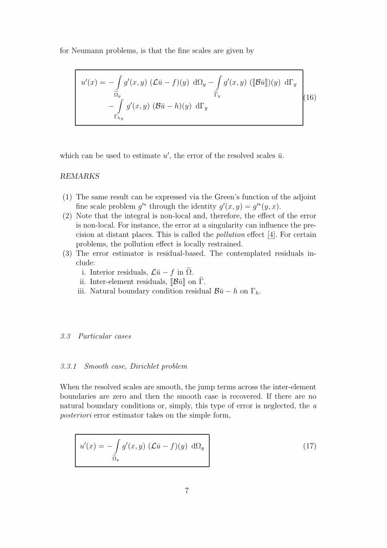
for Neumann problems, is that the fine scales are given by

u′(x) = −∫

Ωy

g′(x, y) (Lu − f)(y) dΩy −∫

Γy

g′(x, y) ([[Bu]])(y) dΓy

−∫

Γhy

g′(x, y) (Bu − h)(y) dΓy

(16)

which can be used to estimate u′, the error of the resolved scales u.

REMARKS

(1) The same result can be expressed via the Green’s function of the adjointfine scale problem g′∗ through the identity g′(x, y) = g′∗(y, x).

(2) Note that the integral is non-local and, therefore, the effect of the erroris non-local. For instance, the error at a singularity can influence the pre-cision at distant places. This is called the pollution effect [4]. For certainproblems, the pollution effect is locally restrained.

(3) The error estimator is residual-based. The contemplated residuals in-clude:

i. Interior residuals, Lu − f in Ω.ii. Inter-element residuals, [[Bu]] on Γ.iii. Natural boundary condition residual Bu − h on Γh.

3.3 Particular cases

3.3.1 Smooth case, Dirichlet problem

When the resolved scales are smooth, the jump terms across the inter-elementboundaries are zero and then the smooth case is recovered. If there are nonatural boundary conditions or, simply, this type of error is neglected, the a

posteriori error estimator takes on the simple form,

u′(x) = −∫

Ωy

g′(x, y) (Lu − f)(y) dΩy (17)

7

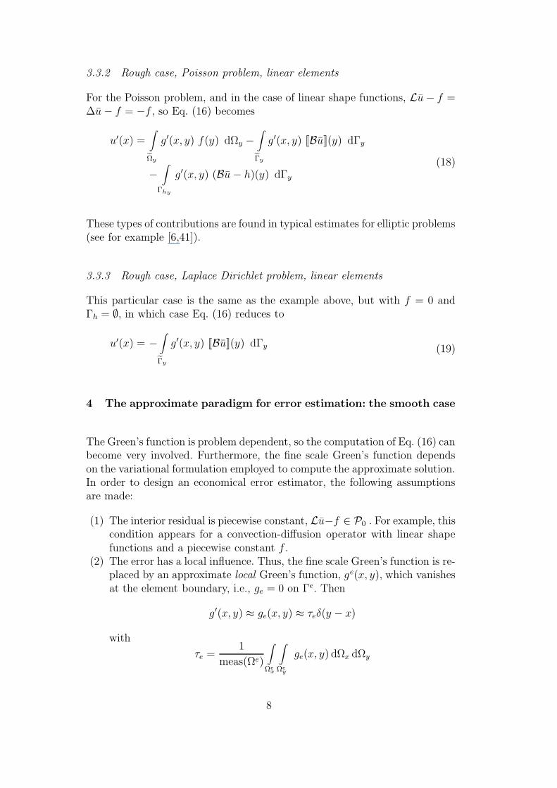
3.3.2 Rough case, Poisson problem, linear elements

For the Poisson problem, and in the case of linear shape functions, Lu − f =∆u − f = −f , so Eq. (16) becomes

u′(x) =∫

Ωy

g′(x, y) f(y) dΩy −∫

Γy

g′(x, y) [[Bu]](y) dΓy

−∫

Γhy

g′(x, y) (Bu − h)(y) dΓy

(18)

These types of contributions are found in typical estimates for elliptic problems(see for example [6,41]).

3.3.3 Rough case, Laplace Dirichlet problem, linear elements

This particular case is the same as the example above, but with f = 0 andΓh = ∅, in which case Eq. (16) reduces to

u′(x) = −∫

Γy

g′(x, y) [[Bu]](y) dΓy (19)

4 The approximate paradigm for error estimation: the smooth case

The Green’s function is problem dependent, so the computation of Eq. (16) canbecome very involved. Furthermore, the fine scale Green’s function dependson the variational formulation employed to compute the approximate solution.In order to design an economical error estimator, the following assumptionsare made:

(1) The interior residual is piecewise constant, Lu−f ∈ P0 . For example, thiscondition appears for a convection-diffusion operator with linear shapefunctions and a piecewise constant f .

(2) The error has a local influence. Thus, the fine scale Green’s function is re-placed by an approximate local Green’s function, ge(x, y), which vanishesat the element boundary, i.e., ge = 0 on Γe. Then

g′(x, y) ≈ ge(x, y) ≈ τeδ(y − x)

with

τe =1

meas(Ωe)

∫

Ωex

∫

Ωey

ge(x, y) dΩx dΩy

8

That is, τe is the element average of the local Green’s function, too. Thisassumption is also implying that the error of the solution is zero in all Γe.As we will see, this hypothesis applies for convection-dominated flows.

REMARK. The above hypothesis yield a stabilized method with nodally exactsolutions for one-dimensional linear problems and piecewise constant residuals[25,19]. In this case, the local Green’s functions represent the fine scales exactlyand, at the same time, the average Green’s function performs exactly thequadrature of the convolution of the unresolved scales onto the resolved scales.

Then, substitution of the above hypothesis yields

u′(x)|Ωe ≈−∫

Ωe

ge(x, y)(Lu− f)(y) dΩy

=−∫

Ωe

τe δ(y − x)(Lu − f)(y) dΩy

=−τe (Lu − f)(x) (20)

Taking the norm,

||u′(x)||2Ωe ≈∫

Ωe

τ 2e (Lu − f)2(x) dΩx

= τ 2e ||Lu− f ||2Ωe (21)

So finally,

||u′(x)||Ωe ≈ |τe| ||Lu− f ||Ωe

= |τe| |Lu − f |√

Ωe(22)

REMARKS

(1) This is a residual-based a posteriori error estimator.(2) It is an estimate of the error in the L2 norm.(3) The method is constant free.

4.1 Relation with bubble-enriched and multi-level methods

Several works have pointed out that there is a relationship between methodsstabilized via bubble functions and stabilized methods (see for example [11]

9

and references therein). In particular, Brezzi et al. [12] show that the space ofresidual-free bubbles for constant residuals can be spanned by the bubble

Lbe = 1 in Ωe

be = 0 on Γe(23)

Under this assumptions, the integral of the local Green’s function is the ele-ment bubble function be(x),

∫

Ωe

ge(x, y) dΩy = be(x) (24)

This fact can be exploited to relate the smooth error estimator with errorestimation based on bubble functions. So for a piecewise constant residual,and neglecting the jump terms, (16) yields for the Dirichlet problem

u′(x)|Ωe =−(Lu − f)∫

Ωe

ge(x, y) dΩy = −(Lu − f) be(x) (25)

Thus,

||u′(x)||Ωe = ||(Lu− f) be(x)||Ωe = |Lu − f | ||be(x)||Ωe (26)

where the last step has been taken assuming piecewise constant residuals.

Russo [37] presented some work on this line based on the H1 norm. Therefore,residual-free bubbles are linked to interior residuals, as suggested by a poste-

riori error estimators based on auxiliary problems. However, error estimationbased on bubbles seems to miss the inter-element residual.

5 Adaptive strategy

In the adaptive process of optimizing the computer resources, given a finiteelement solution on a mesh, the next step is to design the ideal mesh thatwould result in a solution with the desired accuracy. In this work, that isachieved by prescribing the ideal element size as a function of space, leadingto coarsening or refinement.

Given an error tolerance etol = ||u − u||Ωe = ||u′

tol||Ωe (norm of the error in

each element), the norm of the actual error ||u′(i)|| at iteration (i) and the

10

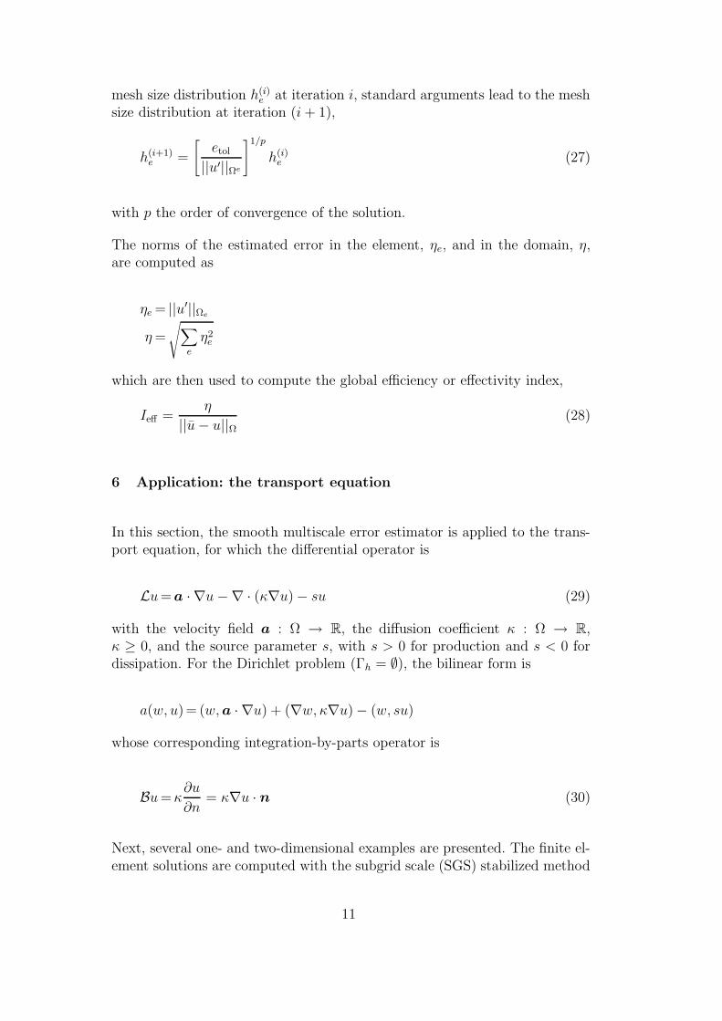
mesh size distribution h(i)e at iteration i, standard arguments lead to the mesh

size distribution at iteration (i + 1),

h(i+1)e =

[etol

||u′||Ωe

]1/p

h(i)e (27)

with p the order of convergence of the solution.

The norms of the estimated error in the element, ηe, and in the domain, η,are computed as

ηe = ||u′||Ωe

η =

√∑

e

η2e

which are then used to compute the global efficiency or effectivity index,

Ieff =η

||u − u||Ω(28)

6 Application: the transport equation

In this section, the smooth multiscale error estimator is applied to the trans-port equation, for which the differential operator is

Lu=a · ∇u −∇ · (κ∇u) − su (29)

with the velocity field a : Ω → R, the diffusion coefficient κ : Ω → R,κ ≥ 0, and the source parameter s, with s > 0 for production and s < 0 fordissipation. For the Dirichlet problem (Γh = ∅), the bilinear form is

a(w, u)= (w, a · ∇u) + (∇w, κ∇u)− (w, su)

whose corresponding integration-by-parts operator is

Bu =κ∂u

∂n= κ∇u · n (30)

Next, several one- and two-dimensional examples are presented. The finite el-ement solutions are computed with the subgrid scale (SGS) stabilized method

11

(also called the unusual stabilized finite element method (USFEM) or theadjoint stabilized method) [17,16,20]. The multiscale error estimator couldbe applied to solutions computed with other finite element methods, like theGalerkin method, but then, the departing hypothesis and the approximationto the fine scale Green’s function could be satisfied to a lesser extent.

The results given by the smooth multiscale method (MS) are compared withthose given by the Zienkiewicz-Zhu (ZZ) method [45]. In order to computethe norms of the exact error, it was seen that the 3rd Gaussian quadraturerule had enough precision.

6.1 One-dimensional numerical examples

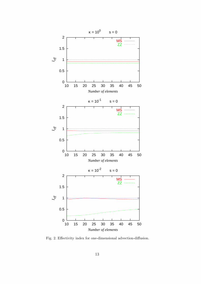
In this section, the effectivity index for increasingly refined uniform meshes oflinear elements is presented for the MS and ZZ methods.

In the multiscale method, the norm of the estimated error is calculated usingthe element residual at the element center. The superconvergent derivativesfor the ZZ method are calculated by averaging the first derivative at eachnode.

6.1.1 Convection-diffusion

The effectivity index of the multiscale method (MS) is compared to the ZZmethod in Figure 2. It can be seen that for a wide range of the diffusioncoefficient κ, the effectivity index of MS is about one, independently of κ. Theresults presented here for the ZZ method are much better than those in [27],yet showing some sensitivity to the diffusivity.

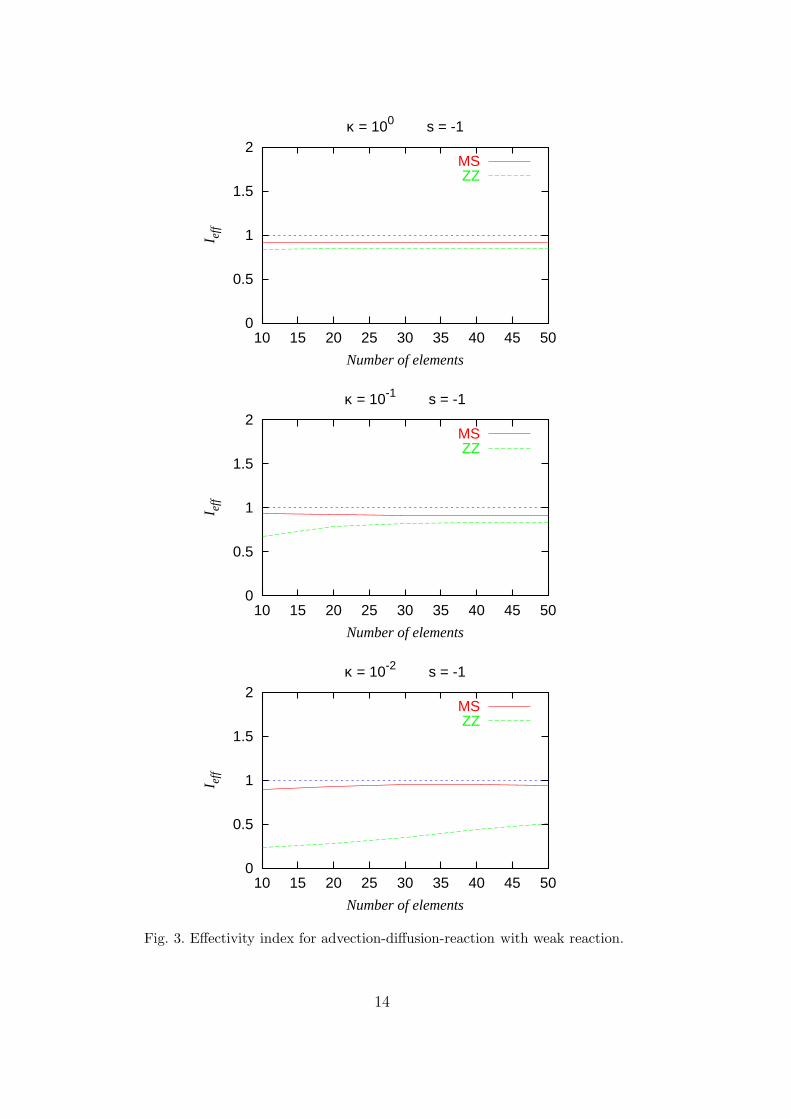
6.1.2 Convection-diffusion-reaction

The results for small reaction s = −1, shown in Figure 3, are very similar tothose with no reaction s = 0.

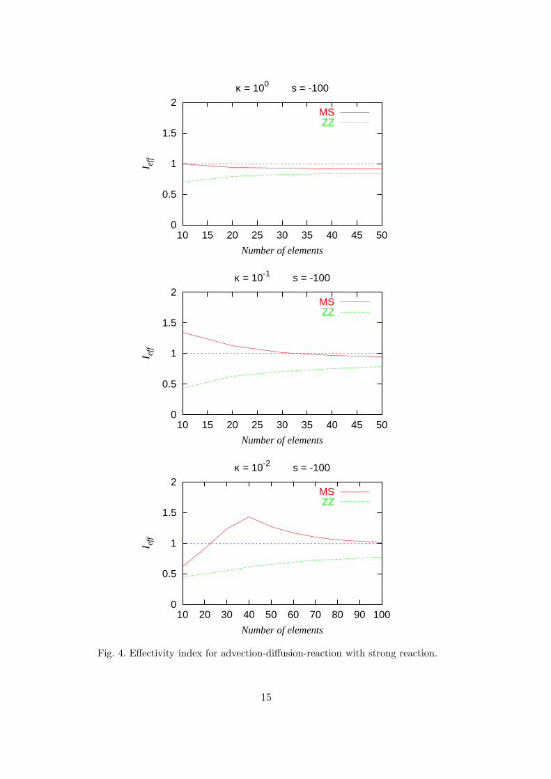
When the reactive term is increased to s = −100, as displayed in Figure 4then the assumption of piecewise constant residual for the MS method startsto fail for coarse meshes. However, as the mesh is refined, the effectivity indextends approximately to one.

For strong reaction, the ZZ error estimator seems less sensitive to the diffusivecoefficient than for the two preceding examples. But in general, the ZZ methodis much less accurate than the MS method.

12

0

0.5

1

1.5

2

10 15 20 25 30 35 40 45 50

I eff

Number of elements

κ = 100 s = 0

MSZZ

0

0.5

1

1.5

2

10 15 20 25 30 35 40 45 50

I eff

Number of elements

κ = 10-1 s = 0

MSZZ

0

0.5

1

1.5

2

10 15 20 25 30 35 40 45 50

I eff

Number of elements

κ = 10-2 s = 0

MSZZ

Fig. 2. Effectivity index for one-dimensional advection-diffusion.

13

0

0.5

1

1.5

2

10 15 20 25 30 35 40 45 50

I eff

Number of elements

κ = 100 s = -1

MSZZ

0

0.5

1

1.5

2

10 15 20 25 30 35 40 45 50

I eff

Number of elements

κ = 10-1 s = -1

MSZZ

0

0.5

1

1.5

2

10 15 20 25 30 35 40 45 50

I eff

Number of elements

κ = 10-2 s = -1

MSZZ

Fig. 3. Effectivity index for advection-diffusion-reaction with weak reaction.

14

0

0.5

1

1.5

2

10 15 20 25 30 35 40 45 50

I eff

Number of elements

κ = 100 s = -100

MSZZ

0

0.5

1

1.5

2

10 15 20 25 30 35 40 45 50

I eff

Number of elements

κ = 10-1 s = -100

MSZZ

0

0.5

1

1.5

2

10 20 30 40 50 60 70 80 90 100

I eff

Number of elements

κ = 10-2 s = -100

MSZZ

Fig. 4. Effectivity index for advection-diffusion-reaction with strong reaction.

15

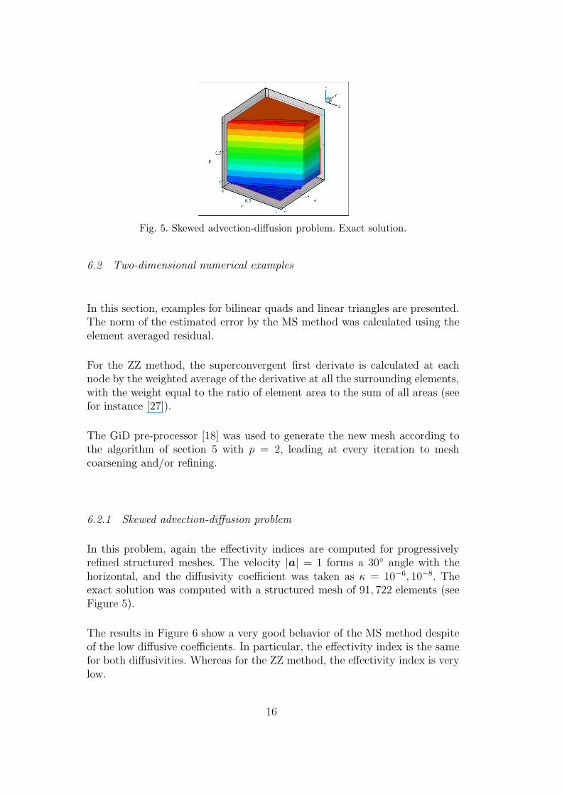
Fig. 5. Skewed advection-diffusion problem. Exact solution.

6.2 Two-dimensional numerical examples

In this section, examples for bilinear quads and linear triangles are presented.The norm of the estimated error by the MS method was calculated using theelement averaged residual.

For the ZZ method, the superconvergent first derivate is calculated at eachnode by the weighted average of the derivative at all the surrounding elements,with the weight equal to the ratio of element area to the sum of all areas (seefor instance [27]).

The GiD pre-processor [18] was used to generate the new mesh according tothe algorithm of section 5 with p = 2, leading at every iteration to meshcoarsening and/or refining.

6.2.1 Skewed advection-diffusion problem

In this problem, again the effectivity indices are computed for progressivelyrefined structured meshes. The velocity |a| = 1 forms a 30 angle with thehorizontal, and the diffusivity coefficient was taken as κ = 10−6, 10−8. Theexact solution was computed with a structured mesh of 91, 722 elements (seeFigure 5).

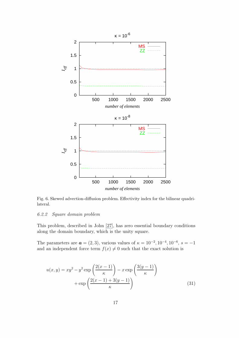
The results in Figure 6 show a very good behavior of the MS method despiteof the low diffusive coefficients. In particular, the effectivity index is the samefor both diffusivities. Whereas for the ZZ method, the effectivity index is verylow.

16

0

0.5

1

1.5

2

500 1000 1500 2000 2500

I eff

number of elements

κ = 10-6

MSZZ

0

0.5

1

1.5

2

500 1000 1500 2000 2500

I eff

number of elements

κ = 10-8

MSZZ

Fig. 6. Skewed advection-diffusion problem. Effectivity index for the bilinear quadri-lateral.

6.2.2 Square domain problem

This problem, described in John [27], has zero essential boundary conditionsalong the domain boundary, which is the unity square.

The parameters are a = (2, 3), various values of κ = 10−2, 10−4, 10−6, s = −1and an independent force term f(x) 6= 0 such that the exact solution is

u(x, y) = xy2 − y2 exp

(2(x − 1)

κ

)− x exp

(3(y − 1)

κ

)

+ exp

(2(x − 1) + 3(y − 1)

κ

)(31)

17

Fig. 7. Square domain problem. Initial mesh.

Fig. 8. Square domain problem. Exact solution.

The initial mesh and the exact solution are plotted in Figures 7 and 8, respec-tively. The prescribed error tolerances are

• MS etol = 5.5 · 10−4

• ZZ needs a variable error tolerance, about e,x tol = 8 · 10−5, to get mesheswith reasonable number of elements

Figure 9 shows the adaptation process with the respective number of elements.The mesh produced by the ZZ method concentrates all the elements near theboundary layers. The MS method produces a graded refinement, catching theslight change of curvature in the middle of the domain.

The effectivity indices are displayed in Figure 10. Again for two-dimensionalproblems, the MS error estimator gives effectivities near one, giving the samevalue for κ = 10−4, 10−6. However, for not so highly advection-dominatedflows (κ = 10−2), the MS error starts to show some sensitivity to the diffusioncoefficient. This could be explained by the contribution of the jump termsto the overall error. For convection-dominated flows, these are negligible, butmay become dominant as the diffusion is increased.

18

MS ZZ

mesh 1 5691 5852

mesh 3 7114 7574

mesh 5 7014 8591

Fig. 9. Square domain problem. Adaptive process for the MS and ZZ methods.

19

0

0.5

1

1.5

2

1 2 3 4 5 6

I eff

Mesh number

κ = 10-2

MSZZ

0

0.5

1

1.5

2

1 2 3 4 5 6

I eff

Mesh number

κ = 10-4

MSZZ

0

0.5

1

1.5

2

1 2 3 4 5 6

I eff

Mesh number

κ = 10-6

MSZZ

Fig. 10. Square domain problem. Effectivity index for the bilinear quadrilateral.

20

Fig. 11. L-shaped domain problem. Initial mesh.

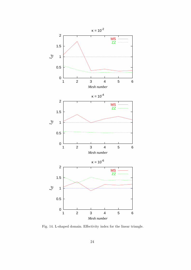
6.2.3 L-shaped domain problem

This problem, described in John [27], has zero essential boundary conditionsalong the domain boundary, which has the shape of an L. The problem issolved with linear triangles.

The parameters of the problem are a = (1, 3), various values of κ = 10−2, 10−4, 10−6,s = −1, and the independent force term f(x)

f(x, y) = 100r(r − 0.5)(r − 1/√

2) (32)

with r2 = (x − 0.5)2 + (y − 0.5)2.

The initial mesh and the exact solution, computed in a mesh of 68, 824 el-ements, are plotted in Figures 11 and 12, respectively. The prescribed errortolerances are

• MS etol = 1.5 · 10−5

• ZZ needs a variable error tolerance, around e,x tol = 1.5 · 10−4, in order toget reasonable meshes with reasonable number of elements

Now, Figure 13 shows the adaptation process. Again, the mesh produced bythe ZZ method concentrates all the elements near the boundary and interiorlayers, however, missing the boundary layer at the right boundary and theoutflow portion of the interior boundary layer. The MS method produces agraded refinement, concentrating elements along all the length of the layers.

The effectivity indices are displayed in Figure 14. Again for two-dimensionalproblems, the MS error estimator gives effectivities near one, giving the samevalue for κ = 10−4, 10−6. However, for not so highly advection-dominatedflows (κ = 10−2), the MS error starts to show some sensitivity to the diffusioncoefficient, which might be indicating the need of including the jump terms inthe smooth a posteriori multiscale error paradigm.

21

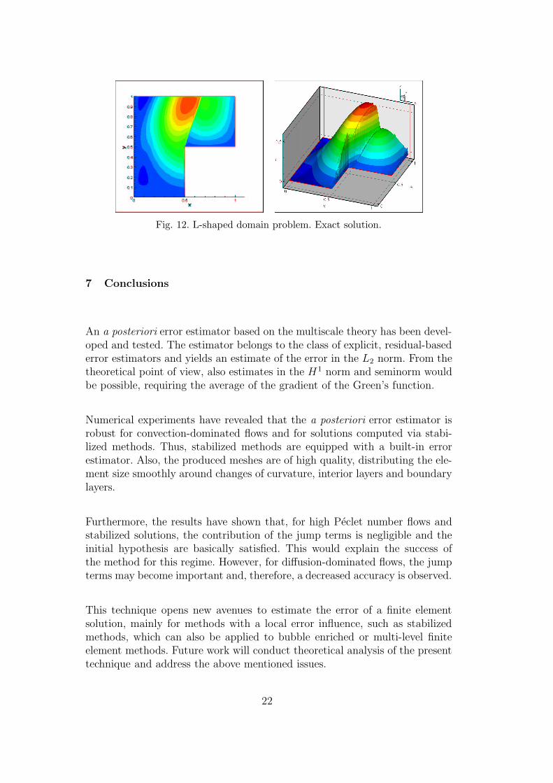
Fig. 12. L-shaped domain problem. Exact solution.

7 Conclusions

An a posteriori error estimator based on the multiscale theory has been devel-oped and tested. The estimator belongs to the class of explicit, residual-basederror estimators and yields an estimate of the error in the L2 norm. From thetheoretical point of view, also estimates in the H1 norm and seminorm wouldbe possible, requiring the average of the gradient of the Green’s function.

Numerical experiments have revealed that the a posteriori error estimator isrobust for convection-dominated flows and for solutions computed via stabi-lized methods. Thus, stabilized methods are equipped with a built-in errorestimator. Also, the produced meshes are of high quality, distributing the ele-ment size smoothly around changes of curvature, interior layers and boundarylayers.

Furthermore, the results have shown that, for high Peclet number flows andstabilized solutions, the contribution of the jump terms is negligible and theinitial hypothesis are basically satisfied. This would explain the success ofthe method for this regime. However, for diffusion-dominated flows, the jumpterms may become important and, therefore, a decreased accuracy is observed.

This technique opens new avenues to estimate the error of a finite elementsolution, mainly for methods with a local error influence, such as stabilizedmethods, which can also be applied to bubble enriched or multi-level finiteelement methods. Future work will conduct theoretical analysis of the presenttechnique and address the above mentioned issues.

22

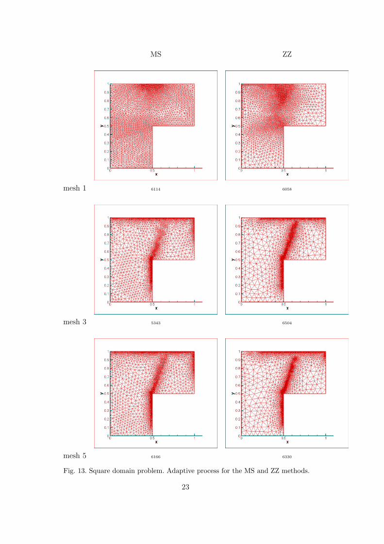
MS ZZ

mesh 1 6114 6058

mesh 3 5343 6504

mesh 5 6166 6330

Fig. 13. Square domain problem. Adaptive process for the MS and ZZ methods.

23

0

0.5

1

1.5

2

1 2 3 4 5 6

I eff

Mesh number

κ = 10-2

MSZZ

0

0.5

1

1.5

2

1 2 3 4 5 6

I eff

Mesh number

κ = 10-4

MSZZ

0

0.5

1

1.5

2

1 2 3 4 5 6

I eff

Mesh number

κ = 10-6

MSZZ

Fig. 14. L-shaped domain. Effectivity index for the linear triangle.

24

Acknowledgements

This work has been partially funded by the Ministerio de Ciencia y Tec-nologıa under contract MCYT TIC2001-2534-C02-01 and Diputacion Gen-eral de Aragon, contract P053/2001. The senior author thanks T.J.R. Hughesand J.R. Stewart for insightful comments. This paper is dedicated to the 60th

birthday of Tom Hughes.

References

[1] M. Ainsworth, A.W. Craig, A posteriori error estimators in the finite elementmethod, Numer. Math., 60 (1991) 429–463.

[2] M. Ainsworth, J.T. Oden, A unified approach to a posterior error estimationusing element residual methods, Numer. Math., 65 (1993) 23–50.

[3] M. Ainsworth, J.T. Oden, A posteriori error estimation in finite elementanalysis, Comput. Meth. Appl. Mech. Engrng., 142 (1997) 1–88.

[4] M. Ainsworth, J.T. Oden A posterior error estimation in finite element analysis,John Wiley & Sons, 2000.

[5] I.M. Babuska, A. Miller, A feedback finite element method with a posteriorierror estimation Part I. The finite element method and some basic propertiesof the a posteriori error estimator, Comput. Meth. Appl. Mech. Engrng., 61(1987) 1–40.

[6] I.M. Babuska, W.C. Rheinboldt, A posteriori error estimates for the finiteelement method, Int. J. Numer. Methods Engrg, 12 (1978) 1597–1615.

[7] I.M. Babuska, W.C. Rheinboldt, Error estimates for adaptive finite elementcomputations, SIAM J. Numer. Anal., 18 (1978) 736–754.

[8] I.M. Babuska, W.C. Rheinboldt, Adaptive approaches and reliabilityestimations in finite element analysis, Comput. Meth. Appl. Mech. Engrng.,17 (1979) 519–540.

[9] I.M. Babuska, W.C. Rheinboldt, Analysis of optimal finite element meshes inR1, Math. Comp., 33 (1979) 435–463.

[10] R.E. Bank, A. Weiser, Some a posteriori error estimators for elliptic partialdifferential equations, Math. Comp., 44 (1985) 283–301.

[11] C. Baiochi, F. Brezzi, L.P. Franca, Virtual bubbles and the Galerkin-least-squares method, Comput. Meth. Appl. Mech. Engrng., 105 (1993) 125–142.

[12] F. Brezzi, L.P. Franca, T.J.R. Hughes, A. Russo, b =∫

g, Comput. Meth. Appl.Mech. Engrng., 145 (1997) 329–339.

25

[13] G. Bugeda, E. Onate, Adaptive mesh refinement techniques for aerodynamicproblems, Numerical Methods in Engineeering and Applied Sciences, Eds.: H.Alder, J.C. Heinrich, S. Lavanchy, E. Onate and B. Suarez, CIMNE, Barcelona,1992.

[14] P. Diez, A. Huerta, A posteriori error estimation for standard finite elementanalysis, Comput. Meth. Appl. Mech. Engrng. 163 (1998) 141–157.

[15] K. Eriksson, C. Johnson, An adaptive finite element method for linear ellipticproblems, Math. Comput., 50 (1988) 361–383.

[16] L.P. Franca, F. Valentin, On an improved unusual stabilized finite elementmethod for the advective-reactive-diffusive equation, Comput. Meth. Appl.Mech. Engrng. 190 (2000) 1785-1800.

[17] L.P. Franca, S.L. Frey, T.J.R. Hughes, Stabilized finite element methods: I.Application to the advective-diffusive model, Comput. Meth. Appl. Mech.Engrng. 95 (1992) 253-276.

[18] GiD, Thepersonal pre/postprocessing system, CIMNE, Barcelona, www.gidhome.com,2003.

[19] G. Hauke, A. Garcia-Olivares, Variational Subgrid Scale Formulations for theAdvection-Diffusion-Reaction Equation, Comput. Meth. Appl. Mech. Engrng.190 (2001) 6847-6865. Erratum: 191 (2002) 3123–3124.

[20] G. Hauke, A simple stabilized method for the advection-diffusion-reactionequation, Comput. Meth. Appl. Mech. Engrng. 191 (2002) 2925-2947.

[21] A. Huerta, P. Diez, Error estimation including pollution assesment for nonlinearfinite element analysis, Comput. Meth. Appl. Mech. Engrng. 181 (2000) 21–41.

[22] T.J.R. Hughes, personal communication, Albuquerque, 2003.

[23] T.J.R. Hughes, The finite element method: Linear static and dynamic finiteelement analysis, Dover Publications, 2000.

[24] T.J.R. Hughes, Multiscale phenomena: Green’s functions, the Dirichlet-to-Neumann formulation, subgrid scale models, bubbles and the origins ofstabilized methods, Comput. Meth. Appl. Mech. Engrng. 127 (1995) 387–401.

[25] T.J.R. Hughes, G.R. Feijoo, L. Mazzei, J.B. Quincy, The variational multiscalemethod: A paradigm for computational mechanics, Comput. Meth. Appl. Mech.Engrng. 166 (1998) 3–24.

[26] H. Jin, S. Prudhomme, A posteriori error estimation of steady-state finiteelement solutionsof the Navier-Stokes equations by a subdomain residualmethod, Comput. Methods Appl. Mech. Engrg., 159 (1998) 19–48.

[27] V. John, A numerical study of a posteriori error estimators for convection-diffusion equations, Comput. Methods Appl. Mech. Engrg., 190 (2000) 757–781.

26

[28] C. Johnson, Adaptive finite element methods for diffusion and convectionproblems, Comput. Methods Appl. Mech. Engrg., 82 (1990) 301–322.

[29] C. Johnson, Finite element methods for flow problems, AGARD Report 787(AGARD, 7 Rue Ancelle, 92299 Neuilly sur Seine, France, (1992) 1-1–1-47.

[30] C. Johnson, P. Hansbo, Adaptive finite element methods in computationalmechanics, Comput. Methods Appl. Mech. Engrg., 101 (1992) 143–181.

[31] D.W. Kelly, J.R. Gago, O.C. Zienkiewicz, I. Babuska, A posterior error analysisand adaptive processes in the finite element method. Part I– Error analysis, Int.J. Numer. Methods Engrg., 19 (1983) 1593–1610.

[32] J.T. Oden, L. Demkowicz, W. Rachowicz, T.A. Westermann, A posteriori erroranalysis in finite elements: The element residual method for symmetrizableproblems with applications to compressible Euler and Navier-Stokes equations,Comput. Methods Appl. Mech. Engrg., 82 (1990) 183–203.

[33] J.T. Oden, W. Wu, M. Ainsworth, An a posterior error estimate for finiteelement approximations of the Navier-Stokes equations, Comput. MethodsAppl. Mech. Engrg., 111 (1994) 185–202.

[34] E. Onate, J. Arteaga, J. Garcıa, R. Flores, Error estimation and mesh adaptivityin incompressible viscous flows using a residual power approach, submitted.

[35] A. Papastavrou, R. Verfurth, A posteriori error estimators for stationaryconvection-diffusion problems: a computational comparison, Comput. MethodsAppl. Mech. Engrg., 189 (2000) 449–462.

[36] M. Paraschivoiu, J. Peraire, A.T. Patera, A posteriori finite element boundsfor linear-functional outputs of elliptic partial differential equations, Comput.Methods Appl. Mech. Engrg., 150 (1997) 289–312.

[37] A. Russo, A posteriori error estimators via bubble functions, MathematicalModels and Methods in Applied Sciences, 1 (1996) 33-41.

[38] J.R. Stewart, T.J.R. Hughes, An a posteriori error estimator and hp-adaptivestrategy for finite element discretizations of the Helmholzt equation in exteriordomains, Finite Elem. Anal. Des. 25 (1997) 1–26.

[39] J.R. Stewart, T.J.R. Hughes, A tutorial in elementary finite elemenet erroranalysis: A systematic presentation of a priori and a posteriori error estimates,Comput. Methods Appl. Mech. Engrg., 158 (1998) 1–22.

[40] T. Strouboulis, J.T. Oden, A posteriori error estimation of finite elementapproximations in fluid mechanics, Comput. Methods Appl. Mech. Engrg., 78(1990) 201–242.

[41] R. Verfurth, A posteriori error estimators for the Stokes problem, Numer. Math.55 (1989) 309–325.

[42] R. Verfurth, A review of a posteriori error estimation and adaptive mesh-refinement techniques, Wiley-Teuber, 1996.

27

[43] R. Verfurth, A posteriori error estimators for convection-diffusion equations,Numer. Math. 80 (1998) 641–663.

[44] J. Wu, J.Z. Zhu, J. Smelter, O.C. Zienkiewicz, Error estimation and adaptivityin Navier-Stokes incompressible flows, Computational Mechanics, 6 (1990) 259–271.

[45] O.C. Zienkiewicz, J.Z. Zhu, A simple error estimator in the finite elementmethod, Int. J. Numer. Methods Engrg, 24 (1987) 337–357.

[46] O.C. Zienkiewicz, J.Z. Zhu, Adaptivity and mesh generation, Int. J. Numer.Methods Engrg, 32 (1991) 783–810.

[47] O.C. Zienkiewicz, J.Z. Zhu, The superconvergent patch recovery and a posteriorierror estimates. Part 1: The recovery technique, Int. J. Numer. Methods Engrg,33 (1992) 1331–1364.

[48] O.C. Zienkiewicz, J.Z. Zhu, The superconvergent patch recovery and a posteriorierror estimates. Part 2: Error estimates and adaptivity, Int. J. Numer. MethodsEngrg, 33 (1992) 1365–1382.

28