Competitive Group Testing and Learning Hidden

Vertex Covers with Minimum Adaptivity∗

Peter Damaschke and Azam Sheikh MuhammadDepartment of Computer Science and Engineering

Chalmers University, 41296 Goteborg, Sweden[ptr,azams]@chalmers.se

Abstract

Suppose that we are given a set of n elements d of which have a property calleddefective. A group test can check for any subset, called a pool, whether it contains adefective. It is known that a nearly optimal number of O(d log(n/d)) pools in 2 stages(where tests within a stage are done in parallel) are sufficient, but then the searcher mustknow d in advance. Here we explore group testing strategies that use a nearly optimalnumber of pools and a few stages although d is not known beforehand. We prove a lowerbound of Ω(log d/ log log d) stages and a more general pools vs. stages tradeoff. This isalmost tight, since O(log d) stages are sufficient for a strategy with O(d log n) pools. Asopposed to this negative result, we devise a randomized strategy using O(d log(n/d)) poolsin 3 stages, with any desired success probability 1 − ε. With some additional measureseven 2 stages are enough. Open questions concern the optimal constant factors andpractical implications. A related problem motivated by, e.g., biological network analysisis to learn hidden vertex covers of a small size k in unknown graphs by edge grouptests. (Does a given subset of vertices contain an edge?) We give a 1-stage strategyusing O(k3 log n) pools, with any parameterized algorithm for vertex cover enumerationas a decoder. During the course of this work we also provide a classification of types ofrandomized search strategies in general.

Keywords: nonadaptive group testing, competitive group testing, combinatorial search,randomization.AMS subject classification: 68Q17 Computational difficulty of problems, 68Q32 Compu-tational learning theory, 68Q87 Probability in computer science, 68W20 Randomized algo-rithms.

1 Background

The group testing problem is to find d elements called positive, or synonymously, defective, ina set X of size n by queries of the following type. The searcher can choose arbitrary subsetsQ ⊂ X called pools, and ask whether Q contains at least one defective. Non-defective elementsare called negative. A positive pool is a pool containing some defective, thus responding Yes

∗This is an extended version of a paper presented at the 17th International Symposium on Fundamentals ofComputation Theory FCT 2009, Wroclaw, Lecture Notes in Computer Science (Springer) 5699, pages 84-95.

1

to a group test. A negative pool is a pool without defectives, thus responding No to a grouptest.

Group testing has several applications, most notably in biological and chemical testing,but also in communication networks, information gathering, compression, streaming algo-rithms, etc., see for instance [9, 10, 15, 20, 21, 22] and further pointers therein.

Throughout this paper, log means log2 if no other base is mentioned. By the information-theoretic lower bound, at least log

(nd

)≈ d log(n/d) pools are needed to find d defectives

even if the number d is known in advance, and it is an easy exercise to devise an adaptivequery strategy using O(d log(n/d)) pools. Here, a strategy is called adaptive if queries areasked sequentially, that is, every pool can be prepared based on the outcomes of all earlierqueries. For many applications however, the time consumption of adaptive strategies is hardlyacceptable, and strategies that work in a few stages are strongly preferred: The pools for everystage must be prepared in advance, depending on the outcomes of earlier stages, and thenthey are queried in parallel.

Any 1-stage strategy needs Ω(d2 log n/ log d) pools, as a consequence of the lower boundfor d-separable matrices [6] which are pooling designs that can distinguish between any twopossible sets of at most d defectives. The same lower bound was already well known ford-disjunct matrices, i.e., special d-separable matrices that also allow very simple decoding ofthe test results [18, 24]. On the other hand, O(d2 log n) pools are sufficient. The currentlybest factor is 4.28; see [8] and the references therein. The first 2-stage strategy using anumber of pools within a constant factor of optimum, more precisely 7.54 d log(n/d), wasdeveloped in [14] and later improved to essentially 4 d log(n/d) [19] and finally 1.9 d log(n/d),or even 1.44 d log(n/d) for large enough d [8]. These strategies use stage 1 to find O(d)candidate elements including all defectives, which are then tested individually in stage 2.Such 2-stage strategies are called “trivial” (a misunderstandable but established term); theyare of independent interest as an intermediate type of strategies between 1-stage and “truly2-stage” strategies. Note that a trivial 2-stage strategy requires no subsequent decoding.

The 2-stage strategies still require the knowledge of an upper bound d on the numberof defectives, and they guarantee an almost optimal query complexity only relative to thisd which can be much larger than the true number of defectives in the particular case. Asopposed to this, adaptive strategies with O(d log(n/d)) pools do not need any prior knowledgeof d. Beginning with [3, 16, 17], substantial work has been done to minimize the constantfactor in O(d log(n/d)), called the competitive ratio. The currently best results are in [25].Our problem with unknown d was also raised in [22], and several batching strategies havebeen proposed and studied experimentally. To our best knowledge, the present work is thefirst to establish rigorous results for this question:

Can we take the best of two worlds and perform group testing without prior knowledge ofd in a few stages, using a number of pools close to the information-theoretic lower bound?This question is not only of theoretical interest. If the number d of defectives varies a lotbetween the problem instances, then the conservative policy of assuming some “large enough”d systematically requires unnecessarily many tests, while a strategy with underestimated deven fails to find all defectives.

It is fairly obvious that a 1-stage strategy cannot do better than n individual tests. Onthe bright side, O(log d) stages are sufficient to accommodate a strategy with O(d log(n/d))pools: Simply double the assumed d in every other stage, and apply the best 2-stage strategyrepeatedly, including a check if all defectives have been found. In this paper we prove that

2

almost log d stages are really needed in the worst case. This clearly separates the complexityof the cases with known and unknown d.

In related work [11] we studied query strategies and the computational complexity oflearning Boolean functions depending on only a few unknown relevant variables. Grouptesting is the special case where the Boolean function is already known to be the disjunctionof the relevant variables.

One modern application of group testing is the reconstruction of biological networks,e.g., protein interaction networks, by experiments that signal the presence of at least oneinteraction in a “pool” of proteins. In some experimental setting, a group test signals thatone fixed protein, called a bait, interacts with some protein in a pool. Hence the problem offinding precisely the interaction partners of a bait is just the group testing problem. Since thedegrees d of vertices in interaction networks are very different and tests are time-consuming,we arrive again at the type of problem discussed above. In [13] we studied a similar prolemwith more powerful, non-binary queries that return all interaction partners of a bait.

Instead of learning a whole graph, i.e., the neighbors of every vertex, we may want tolearn only a small set of vertices that is incident to all edges, that is, a small vertex cover. Ininteraction networks, these vertices can be expected to play a major role, as a small vertexcover represents, e.g., a small group of proteins involved in all interactions [23]. Suppose thatan edge group test is available that tells us, for a pool Q of vertices, whether some verticesin Q are joined by an edge. This assumption is also known as the complex model of grouptesting. Then we encounter the problem of learning a hidden vertex cover: Given a graphwith a known vertex set but an unknown edge set, and a number k, identify a vertex coverof size at most k (or all of them), by using a possibly small number of edge group tests.Learning hidden structures in graphs has been intensively studied for many structures andquery models, we refer to [1, 2, 4] for recent results and a survey. Learning a hidden star [1]is a related but quite different problem.

Note that the vertex cover problem, where the graphs is given and known from thebeginning, is NP-complete, on the other hand, it is a classical example of a fixed-parametertractable (FPT) problem: It can be solved in O(bkp(n)) time, with some constant base b andsome fixed polynomial p. In a sense we will extend the classical FPT result and show thathidden vertex covers can be learned efficiently and nonadaptively if k is small.

2 A Classification of Search Strategies and our Results

We discuss both deterministic and randomized strategies. Traditionally, a randomized al-gorithm is called Monte Carlo if its output is correct with positive probability (that can beboosted close to 1), and called Las Vegas if its output is always correct but the complexity israndomized. Since we are concerned with queries and stages we need a finer classification thatmay be interesting also for other, similar search problems. Regarding the output reliabilitywe distinghuish the following types of strategies, with increasing demands:

PC (probably correct): The output is correct with a given probability 1− ε.PCV (probably correct and verified): Like PC but, additionally, the searcher always knowswhether the output is correct or the algorithm has failed this time.C (correct): The output is always correct.

3

Note that an attribute CV would be meaningless, since C includes by definition that theoutput is verified. Regarding complexity bounds we distighuish:

EQ: The given number of queries is an expected number.GQ: The given number of queries is a guaranteed upper bound.ES, GS: similarly defined, for the number of stages.

We denote types of strategies by these symbols, separated by hyphens. Deterministicstrategies is a special case, with characterization GS-GQ-C. (But conversely, the definitionallows also randomized GS-GQ-C strategies.)

For competitive group testing with O(d log n) queries (i.e., pools), we show the followingresults in this paper:

• For strategies with strict demands we give a lower bound tradeoff for pools vs. stages.In particular, we show that Ω(log d/ log log d) stages are needed to achieve O(d log n)queries. First we prove this for deterministic GS-GQ-C strategies, using a countingargument. (Whereas the technique is fairly standard, the details of the adversarystrategy and counting process are not obvious. We explore a hypergraph representationof the query results. Also, there remains a log log d gap between our current bounds.We conjecture that our proof can be refined to give a matching Ω(log d) lower bound.)

• Then we extend the result to GS-GQ-C strategies. Here the additional idea is to letan adversary speculate on some sequence of pooling designs that appears with positiveprobability, and apply the “deterministic” proof. It remains open whether the lowerbound still holds for GS-EQ-C and ES-GQ-C.

• If we relax some demands, the number of stages goes down to a constant. By estimatingthe unknown number d of defectives in stage 1 and then using a 2-stage strategy, weobtain a GS-EQ-PCV strategy with 3 stages, or alternatively, an ES-EQ-C strategywith 3 + δ stages, where δ can be made arbitrarily small, at cost of the constant factorin the query number O(d log(n/d)).

• The same idea, but combined with randomized 1-stage group testing, yields a GS-EQ-PCV strategy that works in only 2 stages but has a few disadvantages (see details lateron). The complexity of ES-GQ strategies remains open.

• Next we show that competitive group testing with a trivial 2-stage GS-EQ-PCV strategyis impossible (where “trivial” is meant in the above sense).

• If we keep GS-GQ but relax C, we need a non-constant number of stages again, but it isslightly better than the GS-GQ-C lower bound: We give a GS-GQ-PCV strategy with2 log d/ log log n stages, based on random partitions. At first glance it might appearstrange to see n in the denominator, but note that a large n can help the stage numberbecause n appears in the query number O(d log n) as well.

We also highlight some results that came out as byproducts:

4

• From the hypergraph characterization in our lower bound proof we get that determiningthe exact number d of defectives by group tests is not easier than actually identifying thedefectives. (Note that in applications like environmental testing we may only be inter-ested in the amount of contamination of samples, rather than in individual items.) Thiscontrasts to the result that we can approximate d efficiently by randomized strategies(see above).

• As another special case of our pools vs. stages tradeoff, we show that the number ofpools in deterministic strategies with constantly many stages cannot be limited to anyfunction f(d) log n.

Our result for finding hidden vertex covers by edge group tests is only loosely tied to therest and not listed here.

3 A Lower Bound for Adaptivity in Competitive Determinis-tic Group Testing

In this section we give an adversarial answer strategy that forces a certain minimum numberof stages upon a searcher who wants to keep the number of pools restricted. Consider a setX containing an unknown subset of defectives.

Definition 1 Given a set P of pools, the response vector t assigns every positive (negative)pool the value 1 (0). Let P+ and P− be the set of positive and negative pools, respectively.The response hypergraph RH(P, t) has the vertex set V := X \

⋃Q∈P− Q, and every Q ∈ P+

is turned into a hyperedge Q ∩ V of RH(P, t).

The response vector simply describes the outcome of a group testing experiment usingthe set P of pools. The vertices of RH(P, t) are all elements that appear in no negative pool.The hyperedges of RH(P, t) are the positive pools restricted to these vertices, that is, allelements recognized as negative are removed.

A hitting set of a hypergraph is a set of vertices that intersects every hyperedge. Note thata superset of a hitting set is a hitting set, too. From the definitions it follows immediately:

Lemma 2 Let t be a given response vector. Then a subset of X is a candidate for being theset of defectives if and only if it is a hitting set of RH(P, t).

Before we state our adversary strategy in detail, we outline the ideas. Consider anydeterministic group testing strategy that works in stages. Our adversary answers the queriesin every stage in such a way that RH(P, t) has some hitting set that is much smaller than thevertex set. This leaves the searcher uncertain about the status (positive or negative) of all theother vertices in RH(P, t). (Note that an adversary working against a deterministic searchercan hide defectives after having seen the pools.) Next, we use a standard trick to simplifythe analysis: The adversary may cautiously reveal some extra information. Specifically, ouradversary tells the searcher a subset of defectives that forms already a hitting set of RH(P, t).The effect is that all hyperedges of RH(P, t) are now “explained” by the revealed defectives,thus RH(P, t) does not contain any further useful information for the searcher. Hence the

5

searcher can totally forget the hypergraph, and the searcher’s knowledge is merely representedby two sets: the already known defectives, and the elements whose status is yet unknown.Each of the latter elements can be (independently!) positive or negative. We will play aroundwith the cardinalities of these two sets and make the searcher’s life as hard as possible. Inthe following we specify our adversary strategy in detail.

Let f be any monotone increasing function and d the true number of defectives. Recallthat d is unknown to the searcher. Suppose that the searcher is aiming for at most f(d) log nqueries in total. Let us consider the moment prior to any stage. Suppose that k defectivesare already known and u elements are yet undecided. As we might have d = k, the searchercan prepare a set P of at most f(k) log n pools for the next stage. (Actually, the number ofpools already used up in earlier stages must be subtracted, which makes the limit even lower,but our analysis does not take advantage of this fact.) These queries in P can generate atmost 2f(k) log n = nf(k) different response vectors. The adversary chooses some number h ≤ uand announces that at least h of the u undecided elements are also defective. In particular,there exist

(uh

)possible sets of exactly h further defectives. By the pigeonhole principle, some

family T of at least(uh

)/nf(k) of these candidate sets of size h generate the same consistent

response vector t. Now the adversary answers with just this response vector t. Let Y denotethe union of all sets in T .

Lemma 3 Y is entirely in the vertex set of RH(P, t).

Proof. Assume that some q ∈ Y is in some pool Q which is negative in t, that means,t(Q) = 0. By the definition of Y , element q also belongs to some Z ⊆ Y such that responsevector t is generated if Z is the actual set of defectives. This contradicts Q ∩ Z = ∅.

Define y = |Y |. Finally, the adversary actually names a set H of h new defectives in Y ,in compliance with t. By Lemma 2, H is a hitting set in RH(P, t). Since arbitrary supersetsof H are hitting sets, too, and Y is included in RH(P, t) by Lemma 3, it follows that H plusany of the y−h elements of Y \H build a hitting set of RH(P, t). Using Lemma 2 again, weconclude that the y − h elements of Y \H are still undecided, that is, they may be defectiveor not, independently of each other.

Since Y must contain at least(uh

)/nf(k) different subsets of size h, we get the following

chain of inequalities:yh

h!>

(y

h

)≥

(uh

)nf(k)

>(u− h)h

h!nf(k).

Multiplication with h! and taking the h-th root yields y > (u− h)/nf(k)/h.In summary, after the considered stage the searcher knows k + h defectives, and at least

y − h > (u− h)/nf(k)/h − h = u((1− h/u)/nf(k)/h − h/u) elements remain undecided. Thuswe update k, u by k := k + h and u := y− h. This concludes the discussion of any one stage.

In the following, s denotes the number of stages the adversary wants to enforce, ki and ui

indicates the value of k and u, respectively, before stage i, and hi is the value of h in stage i.The adversary will choose the hi in such a way that us is still positive. Her choice of numbershi > f(ki) will be based on f(ki) only.

Remember that the function f is fixed. This allows us to neglect some minor terms inthe expression for the updated u without affecting the asymptotics: Since k ≤ d holds at anytime, the largest possible f(k) depends on d only. Furthermore, since our adversary chooses

6

in every stage h > f(k) depending on f(k) only, the ratios h/u in the above expressionfor y − h remains bounded by an arbitrarily small constant all the time, when we start atlarge enough n. Therefore we can assume for simplicity that at least u/nf(k)/h elements areundecided after the considered stage. The relative error becomes arbitarily small as n grows.

Let k1 = 1, that is, one defective is revealed in the beginning. We let our adversary choosethe hi such that

∑i f(ki)/hi ≤ 1 after any number i ≤ s of stages. Since u1 = n − 1 and

ui+1 ≥ ui/nf(ki)/hi , we have that ui remains positive for i ≤ s, as desired.Specifically, let hi := sf(ki) for all i, hence f(ki)/hi = 1/s and ki+1 = ki+hi = ki+sf(ki).

Now we can formulate a somewhat technical but general result:

Theorem 4 Let f be any monotone increasing function with f(d) ≥ d for all d. Any deter-ministic group testing strategy that uses, for arbitrary combinations d, n, at most f(d) log npools for finding a previously unknown number d of defectives out of n elements, needs atleast s(d) stages in the worst case, where s(d) is defined as the minimum number with thefollowing property: If the operator k := k + sf(k) is iterated s := s(d) times starting fromk = 1, then k ≥ d is reached.

Theorem 4 in this general form looks bulky, but for the most important cases of functionsf we get some interesting results from it. First we look at f(d) = d. Due to the information-theoretic lower bound for group testing, this is the smallest meaningful function f in ourcontext.

Corollary 5 Any deterministic group testing strategy that uses, for arbitrary combinationsd, n, only O(d log n) pools for finding a previously unknown number d of defectives out of nelements needs Ω(log d/ log log d) stages in the worst case.

Proof. With the previous denotations, f(k) = k yields ki+1 = (s + 1)ki, hence d = ks+1 =(s + 1)s, and s > log d/ log log d.

We remark that raising the number of pools by a constant factor a does not help verymuch: Since now f(k) = ak, our adversary chooses k := (as + 1)k and still achieves s =Θ(log d/ log log d), although with a smaller constant factor.

Next it is interesting to consider f(d) = d2, because this number of pools would allow a1-stage strategy if d were known beforehand (see Section 1). However, our adversary strategyfor unknown d essentially squares k in every iteration, leading to s = Ω(log log d). Finally,consider an arbitrary but fixed function f that may be rapidly growing.

Corollary 6 Let f be any monotone increasing function. No deterministic group testingstrategy that uses at most f(d) log n pools for finding a previously unknown number d ofdefectives out of n elements can succeed in constantly many stages.

Proof. It suffices to notice in Theorem 4 that the number s of iterations needed to reachk ≥ d depends on d.

This contrasts sharply to our result in the next section where we give randomized strate-gies with constantly many stages, based on a randomized estimate of d. A simple but inter-esting observation in this context is that finding the exact number of defectives is not easierthan solving the whole group testing problem:

7

Theorem 7 Any group testing strategy that exactly determines the previously unknown num-ber of defectives must also identify the set of defectives.

Proof. Assume that a searcher has applied any group testing strategy to some set of elementscontaining d defectives, and afterwards the searcher knows d. Let P be the set of pools everused, and t the response vector. By Lemma 2, the possible sets of defectives are exactly thehitting sets of RH(P, t). Hence, by assumption, all hitting sets of RH(P, t) have the samecardinality. This is possible only if RH(P, t) has only the trivial hitting set consisting of allvertices. Using Lemma 2 again, it follows that the searcher knows the defectives.

So far we have studied only deterministic strategies. Recall that they are of type GS-GQ-C. Next we show that the general Theorem 4 (and hence the subsequent results) still holdsfor randomized strategies of this type. Note that the adversary has to be “oblivious”, i.e.,she must fix the set of defectives before seeing the searcher’s random decisions.

Theorem 8 Let f be any monotone increasing function with f(d) ≥ d for all d. Any GS-GQ-C group testing strategy that uses, for arbitrary combinations d, n, at most f(d) log npools for finding a previously unknown number d of defectives out of n elements, needs atleast s(d) stages, with s(d) defined as in Theorem 4.

Proof. Consider any randomized strategy. We let our adversary from Theorem 4 play againstthe strategy. The possible outcomes can be viewed as a tree, in an obvious way: In every treenode the searcher decides on the set of pools for the next round, with probabilities specifiedby the strategy, and then our adversary reacts as above. Now, if the strategy is GS-GQ-C, itmust succeed on any path of the tree, i.e., identify the defectives correctly within the specifiedbounds for stages and pools.

The above procedure describes an adaptive adversary that can decide on further defectivesstep by step according to the searcher’s choices. However, an oblivious adversary can chooseany path p of the tree and speculate that the searcher will behave as on p (which happens withpositive probability), and choose the set of defectives according to the result of p. Then thesequence of pools used on p can be seen as a deterministic strategy (applied by the searcherwith some positive probability), and Theorem 4 shows that, on p, the searcher cannot workcorrectly and stick to both complexity bounds at the same time. Hence one of the constraintsis violated with positive probability, thus a GS-GQ-C strategy with f(d) log n pools and lessthan s(d) stages cannot exist.

We conjecture that the same lower-bound tradeoff still holds for each of the weaker de-mands GS-EQ-C and ES-GQ-C. It is tempting to argue as follows: If a strategy respects anexpected value of one complexity bound (and the other bound is strict), then the concretevalue on some tree path p must not exceed the expectation, and Theorem 4 shows again thatthe strategy cannot work correctly on p. However, the catch is that the expectation in EQor ES refers to the searcher’s behaviour on any set of defectives fixed beforehand, hence theadversary cannot simply speculate on p as in the GS-GQ-C case.

4 Randomized Estimation of the Number of Defectives

In this section we show that a “conservative bound” d on the number d of defectives in aset of n elements can be determined by O(log n) randomized nonadaptive group tests. What

8

the above phrase means is that we get d < d with an arbitrarily small prescribed failureprobability, but d overestimates d only by a constant expected factor. Thus, d can be furtherused in any group testing strategy that needs an upper bound on d: Such a strategy failsonly with a small probability due to d < d, but it is also unlikely to waste too many testsdue to a large d/d.

Let b > 1 be a fixed positive real number. We prepare a sequence of pools indexed byintegers i as follows. We put every element independently with probability 1 − (1 − 1/n)bi

in the ith pool. The ith pool is negative with probability qi := (1 − 1/n)dbi, since this is

the probability that all d defectives are outside the pool. The test outcomes of all pools areindependent, as we have chosen the elements of the pools independently. Also note that,regardless of the unknown value of d, our sequence qi is doubly exponential: Every numberis the bth power of the previous number and the bth root of the next number. This is a niceinvariant that enables a “uniform” analysis for all possible values of d.

Let e denote Euler’s number and k := blogb nc. We have q0 = (1− 1/n)n ≈ 1/e if d = n,and qk ≈ (1 − 1/n)n ≈ 1/e if d = 1. That means, q0 is “away from” 0 even if d = n, andqk is “away from” 1 even if d = 1. Now let i range from some constant negative index to kplus some positive constant. Then group testing on this sequence of pools yields, with highprobability, some negative pools in the beginning, even if d = n, and some positive pools inthe end, even if d = 1. Notice that we prepare roughly logb n = log n/ log b pools.

We propose a simple algorithm to get d from the test outcomes. It is equivalent to estimatethe index j of a pool with some fixed value qj . Our algorithm will “assume” qj = 1/2 for acertain j based on the test outcomes, and output the corresponding number of defectives dthat would lead to qj = 1/2. In order to distinguish this assumed probability value from thetrue (and unknown) qj we denote it qj . Our algorithm uses yet another positive parameters (integer) that we discuss later. The subsequent lemmas are meant with respect to thealgorithm. Here it is:

Let i be the largest index of a negative pool; we will referto i as the main index. Then let qi−s := 1/2 and set daccordingly, that is, d := −1/(bi−s log(1− 1/n)).

(Clearly d must be rounded to an integer, for simplicity we omit ceiling brackets.) Re-member that b > 1 is some fixed base. We choose s large enough to make 1/2bs

“small”, seethe details below. With these presumptions we get:

Lemma 9 The probability of d < d is O(1/2bslog b).

Proof. The event d < d is equivalent to qi−s < 1/2 for the main index i. In this case, i is oneof the indices with qi < 1/2bs+j

, j ≥ 0. Hence the probability of this failure is bounded by∑j≥0 1/2bs+j

. Since 1/2bsis already small due to the choice of s, and every term is the bth

power of the previous one, the sequence then decreases rapidly: After every logb 2 = 1/ log bindices it is reduced to the square. Thus we get a failure probability as claimed, with a smallhidden constant.

9

In order to express the expected competitive ratio we define a function F with argumentb > 1 by:

F (b) := max0≤θ<1

∞∑i=−∞

b−i+θ

2bi−θ

∞∏k=1

(1− 1

2bi−θ+k

).

Although the expression for F (b) looks complicated, it is not hard to prove that F (b) ismonotone in b, and to get good simple bounds for F (b). However, we do not further analyzeF , as these issues affect only the constant factors in our final results below. Instead, somenumerical values may illustrate the behaviour of F :

#pools 1 log n 2 log n 4 log n 8 log n 16 log n 32 log n

b 2.000 1.414 1.190 1.091 1.045 1.022F (b) 1.466 0.830 0.549 0.397 0.307 0.247

Lemma 10 The expectation of d/d is at most F (b) · bs.

Proof. We (arbitrarily) shift our indices such that 1/2b−1> q0 ≥ 1/2b0 and define θ such

that 0 ≤ θ < 1 and q0 = 1/2b−θ. If the main index is i, the algorithm yields qi−s = 1/2

whereas qi−s := 1/2bi−s−θ, hence d/d = b−i+θ · bs. From qi = 1/2bi−θ

and the definition of themain index, the assertion follows.

Altogether we have shown:

Theorem 11 Consider a set of n elements including an unknown number d of defectives.For any b > 1 and any positive integer s, there is a randomized 1-stage group testing strategywith log n/ log b pools that outputs a number d such that d < d holds only with probabilityO(1/2bs

log b), and d/d < F (b) · bs in expectation.

5 Randomized Competitive Group Testing in Two or ThreeStages

From the result of the previous section we can easily conclude:

Theorem 12 Consider a set of n elements including an unknown number d of defectives.(i) There is a GS-EQ-PCV group testing strategy that finds all defectives in 3 stages usingO(d log(n/d)) pools.(ii) For any fixed δ > 0 there is a ES-EQ-C group testing strategy that finds all defectives in3 + δ stages using O(d log(n/d)) pools.

Proof. Fix any desired failure probability bound ε > 0. By Theorem 11 we can get in stage 1some d that exceeds d with probability at least 1− ε, keeping the expected ratio d/d constantat the same time, and O(log n) pools are used for that, where the constant factor dependson ε. Then we apply one of the established 2-stage group testing strategies for a maximumnumber d of defectives. As mentioned in Section 1, there are 2-stage strategies that firstdetermine O(d) candidate elements including all defectives, and test them individually in the

10

final stage. We add one more pool in this final stage, consisting of the complement of thecandidates. If this extra pool is negative, the searcher knows that all defectives are found,hence the strategy is PCV. (But it can still fail if d < d.) This shows (i). Assertion (ii) is asimple extension: If failure is detected in stage 3, the strategy is repeated until success. Weachieve any desired δ by chosing ε small enough.

Some practical remarks are in order here: Since the probability of a too generous ddecreases rapidly as the ratio d/d grows, large deviations from the expected number of poolsare very unlikely. On the other hand, note that d/d is not necessarily close to 1. The bestchoice of the method parameters b, s that minimize, e.g., the hidden factor in O(d log(n/d))depends on ε and the largest relevant d. This needs to be further explored. We did somenumerical experiments adopting the 1.44 d log(n/d) bound for 2-stage group testing [8]. Withbases 1.2 < b < 1.5 we get factors from 3 + 1/d log b to 6 + 1/d log b, for ε from 0.1 down to0.02.

Next we show that even two stages are enough if we randomize the further tests as well.In Theorem 10 of [8] it is shown that up to d defectives can be identified correctly, withany desired constant probability, in one stage using O(d log n) pools. Inspection of the proofshows that their random set of pools has, with constant probability, the following property:Let P be the set of positive elements. If actually |P | ≤ d then, (i) for every v /∈ P there existsa negative pool that contains v but is disjoint to P . The same analysis in [8] also shows that,(ii) for every v ∈ P , there exists a positive pool Q that contains v but is disjoint to P \ v.The strategy outputs all elements that appear in positive pools only. The above propertiesimply that, with constant probability, every negative element v is recognized as negative dueto (i), and every positive element v is recognized as positive due to (ii). The latter statementholds since Q is a positive pool but all elements in Q \ v are recognized as negative. Inother words, the output set O is exactly P in this event. From the searcher’s point of viewwe have: If O (in the role of P ) satisfies (i) and (ii) then the searcher is sure about O = P .Hence this strategy is PCV.

Theorem 13 Consider a set of n elements including an unknown number d of defectives.There is a GS-EQ-PCV group testing strategy that finds all defectives in 2 stages usingO(d log n) pools.

Proof. As before, fix any desired failure probability bound ε > 0 and determine in stage 1some d that is smaller than d with probability at most ε/2, and with constant expected ratiod/d. In stage 2, apply a the 1-stage PCV strategy for d defectives and failure probability ε/2.Thus the strategy fails with probability at most ε, and if it succeeds, the searcher knows thatexactly the set of positive elements has been returned.

Thus we have saved one stage, but we conjecture that the hidden constant factor inO(d log n) will be considerably larger than for 3 stages, mainly since the error probability εmust be divided between two stages (whereas in Theorem 12 only stage 1 could potentiallyfail). We must leave the constant factors, depending on the prescribed ε, as an open question.Obviously, the 2-stage strategy also needs a larger amount of randomness.

A clear disadvantage of the 2-stage strategy is in the verification step. While the proposed3-stage strategy really ends after the tests in stage 3, the 2-stage strategy needs quite somecomputational postprocessing to confirm the result: It guarantees a correct result only if the

11

output set O has the above properties (i) and (ii), that is, we have to revisit the pool set andfind the required pools for every element v. A natural question is whether a trivial 2-stagestrategy exists with the same performance. Remember that a 2-stage group testing strategyis called trivial if stage 2 consists of individual tests of candidate positives only, hence nodecoding or verification is needed at all. However we can show:

Theorem 14 There exists no trivial 2-stage GS-EQ-PCV strategy for group testing withpreviously unknown d, using O(d log n) pools.

Proof. Since such a strategy has to test all candidates from stage 1 individually in stage 2,the total number of pools is at least the number of candidates from stage 1.

First we prove the assertion for GS-GQ-PCV strategies. Suppose that the searcher wantsto use at most cd log n pools, for some constant c. Regardless of her random choices thesearcher may use only c log n pools in stage 1, since otherwise the adversary may simplyfix d = 1. It remains to show that the number of candidates remains too large after thesec log n nonadaptive group tests. As the pooling design may be randomized, we use Yao’stechnique to derive a lower bound on the expected number of candidates. We say that anegative pool discards the elements in this pool. First consider any deterministic, i.e., fixedpooling design in stage 1. Our adversary fixes some number d (we discuss the choice ofd below) and decides d defectives at random. Thus, any pool of size xn is negative withprobability (1 − x)d, that is, the pool discards an expected number of x(1 − x)dn elements.By a standard calculation, this expectation is maximized if x = 1/(d+1), hence the expectednumber of elements discarded by any one pool is at most n/e(d+1), where e denotes Euler’snumber. By linearity of expectation, c log n pools discard an expected number of at most(cn log n)/(e(d + 1)) elements. (Actually this number is smaller if the pools overlap.) If d ischosen larger than (c/e) log n, there remain Ω(n) expected candidates when any deterministicstrategy is applied in stage 1. Any randomized pooling design using a fixed number of c log npools in stage 1 is a probability distribution on the deterministic pooling designs of that size.Hence, with d > (c/e) log n random defectives, Ω(n) expected candidates are left, also if sucha randomized design is applied. It follows that some specific set of d > (c/e) log n defectivesexists that fools the given randomized strategy.

Finally we consider GS-EQ-PCV strategies. Now the searcher may also randomize overthe number of pools to be used in stage 1, but still their expected number must not exceedc log n, for the same reason as above. For any fixed ε > 0, Markov’s inequality yields thatthe strategy must choose the actual number of pools below (1 + ε)c log n with some constantpositive probability. Applying the previous result to this event we see that the expectednumber of candidates remains Ω(εn) there. Thus, with constant positive probability thesearcher is faced with Ω(εn) candidates to test in stage 2, which in total enforces a linearexpected number of pools.

Note that this proof uses that possibly d = Ω(log n). If d is smaller compared to log n,we can again succeed with O(d log n) pools in 2 stages, even with a GS-GQ-PCV strategy.However, we prove a more general result below.

Lemma 15 Consider a set of m elements. There exists a GS-GQ-C strategy using O(log m)pools in 1 stage, that finds the defective if d = 1, and otherwise recognizes that d = 0 or d > 1.

12

Proof. Let n be a power of 2, otherwise we create dummy elements, which doubles m in theworst case. We arrange the elements in a log m dimensional hypercube and query its 2 log mmaximal subhypercubes. If actually d = 1, the answers obviously determine the defectiveuniquely. If d = 0 then all pools are negative. If d > 1 then at least two complementarypools are positive. These cases are recognized by the searcher.

Theorem 16 Consider a set of n elements including an unknown number d of defectives.There exists a GS-GQ-PCV strategy using O(d log n) pools in O(log d/ log log n) stages.

Proof. Every stage works as follows: If h is a currently known lower bound for d (whereh = 1 is assumed in the beginning), we partition the elements randomly into some Θ(h log n)disjoint pools of equal size and query them. For the next stage we update h as the numberof positive pools.

Using simple standard results from probability theory, the following two things happenwith high probability: As long as h log n < d, at least a constant fraction of pools answerspositively, thus h is multiplied by Θ(log n) in every stage. As soon as h log n > d2, thedefectives are separated, that is, no two defectives get into the same pool.

In the latter case the searcher recognizes that fewer than√

h log n pools are positive andconjectures that the defectives are in fact separated. Finally, in one further round the searcherapplies Lemma 15 to each positive pool from the previous stage, to find the defective andconfirm that it is the only one.

As for the stage number, note that s = log d/ log log n is the solution to (log n)s = d, andconstant factors are captured by the O-notation.

In particular, this algorithm uses only 2 stages if d = O(√

log n). It would be interestingto explore the case when

√log n < d < log n.

6 Learning Hidden Vertex Covers by Edge Group Tests

In this section we study the problem of learning all minimal vertex covers of size at most k,in an initially unknown graph, from edge group tests. Note that, in general, this does notuniquely determine the graph, because there may exist further minimal vertex covers withmore than k vertices.

Definition 17 A set of pools is (2, k)-disjunct if, for any k + 2 vertices w1, . . . , wk and u, v,there exists a pool that includes u, v and excludes w1, . . . , wk.

There exist (2, k)-disjunct matrices with O(k3 log n) pools: The simplest randomizedconstruction is to put every vertex in a pool independently with probability 2/k. Bounds onthe size of a more general type of disjunct matrices can be found in [5].

Let V C(n, k) denote the time for enumerating the minimal vertex covers of size at mostk in a (known!) graph of n vertices. The time depends on the state-of-the-art of FPT vertexcover algorithms, which is beyond the scope of this work. However, we have V C(n, k) =O(bkp(n)) where b < 2 is some fixed base and p some fixed polynomial, see [12] for moredetails. If only one vertex cover is sought, one can apply faster algorithms such as the one in[7].

13

Theorem 18 We can learn all (minimal) vertex covers of size at most k in one stage usingO(k3 log n) edge group tests and O(V C(n, k)) time for auxiliary computations. The strategyis of type GS-GQ-C.

Proof. We take a set of pools that forms a (2, k)-disjunct matrix. Consider any pair ofvertices u, v. Clearly, if u, v belongs to some negative pool then uv is a non-edge. Theother case is that u, v belongs to positive pools only. Assume that u, v /∈ C for some vertexcover C with |C| ≤ k. Due to (2, k)-disjunctness, some pool includes u, v and excludes C.This pool must be positive, as it contains u, v. On the other hand, the pool must be negative,as every edge intersects C. This contradiction shows that every vertex cover C with |C| ≤ kcontains u or v. Hence, for the purpose of learning these small vertex covers, we may simplyassume that uv is an edge if u, v appears in positive pools only. This might be wrong inthe unknown graph, but the family of vertex covers of size at most k is preserved.

This reasoning also yields the following parameterized decoding algorithm that actuallygenerates the family of vertex covers of size at most k from the test outcomes: Constructan auxiliary graph where uv is an edge if and only if u, v belongs to positive pools only.This can be done in O(k3n2 log n) time, which is dominated by the time for the final step:Compute the minimal vertex covers of size at most k in this graph.

On the other hand, the trivial information-theoretic lower bound gives:

Proposition 19 Any strategy (which may even be adaptive) for learning hidden vertex coversof size at most k needs Θ(k log(n/k)) edge group tests.

An obvious question is what is the best exponent of k in the query number O(kO(1) log n),depending on the number of stages and the type of strategy. In Theorem 18 we did not useprior knowledge of the size of a smallest vertex cover. If our k is too small, we just obtain anempty result which is correct. However, if we want some vertex cover, we have to determinethe minimum size k of a vertex cover first. Here, an O(log k)-stage deterministic strategy ora randomized 1-stage method similar to Section 4 should work. Note that the complementsof vertex covers in a graph are exactly the independent sets, which in turn corresponds tonegative pools. Hence we could again use a randomized sequence of pools of exponentiallygrowing size to estimate k. We have to leave these questions for further research.

7 Some Discussion and Experimental Findings

Besides the open problems regarding strategy types and asymptotic complexity results (men-tioned at several places), more research is needed on the practical side:

Our current lower bounds in Section 3 do not say too much about realistic problem sizes,but we conjecture that they can be further raised. An obvious weakness in the analysisin Section 3 is that the searcher is allowed to use the maximum number of pools in everynew stage, not counting the pools used up earlier. Asymptotically this is negligible, butfor moderate d our adversary gives away some power by this simplification. One may alsothink of more sophisticated adversary strategies that exploit more structure of the responsehypergraphs.

14

Our d in Section 4 is, for the sake of simplicity, based on the “main index” i only, whichis the index of the largest negative pool. This strategy is very sensitive to the position of themain index which may easily be an outlier. In order to get more robust estimates we haveempirically tried different rules of combining the responses of pools around the main index.Here we summarize a comparison with two other natural rules that show significantly betterperformance. The rules differ in the choice of pool j for which we assume qj := 1/2.

Rule 1: the simple algorithm analyzed in Section 4, with j = i− s for some previously fixeds that depends on the desired failure probability bound.Rule 2: like Rule 1, but j is the index of the s-th negative pool before i, jumping over thepositive pools.Rule 3: Let k be the index of the smallest positive pool, m = b(i + k)/2c, and finally, j bethe index of the s-th negative pool before m.

The rationale behind Rule 2 is that it suppresses a too large main index i (an outlier)by straight going to the previous negative pools, and the averaging in Rule 3 should have asmoothing effect as well.

We implemented these rules in Matlab and performed extensive simulations with inde-pendent random choices of d defective elements. Recall from Section 4 that b > 1 is somefixed base used in the sequence of pool sizes. We considered all values of b in the range1.1 to 1.9 with an increment of 0.1. For fixed n we selected d as 0.01n to 0.10n with 0.01nincrements. Now for different b we separately organized simulation results over the range ofs values. Then we computed average values for failure probability, competitive ratio, andvariance in competitive ratio values. To compare the performance of the three rules, we havedrawn graphs of competitive ratios and variances against failure probability (smaller than0.1) for each b. For this purpose, in every rule only those s values are considered where theaverage failure probability lies within the desired range. Here we display competitive ratios(Figure 1–3) and variances (Figure 4–6) for b values 1.1, 1.3, and 1.5. Symbols ×,+, and ∗are used to draw points for rules 1,2, and 3, respectively. Integers besides the points indicatethe values of s. The measured points are joined using the logarithmic curve fitting just forbetter visualization of the behaviour, this is not meant to be interpolation.

The following conclusions can be drawn. Rule 2 has shown consistently better performanceboth in competitive ratio and variance compared to the other two rules. It decreases theaverage competitive ratio by 20% and the variance by 50% or more compared to Rule 1, forany given failure probability, whereas a significant improvement over Rule 3 is also achieved.For both Rule 2 and 3, the improvement in the competitive ratio compared to Rule 1 increasesas the failure probability approaches zero. A close look at the entire simulation data alsoreveals that Rule 3 has consistently gained failure probability less than 0.08 with competitiveratio in the range 2 to 3 already for s = 0, in contrast to Rule 1 that requires large jumps s toachieve small failure probabilities. Overall these simulations suggest that the new rules offera better performance. An obvious plan is to analyze and understand them also in theory andto figure out the best hidden constants we can achieve in Theorem 12.

Some other ideas for further research on this topic came up:We invented Rule 2 and 3 by ad-hoc considerations and then tested them. In principle

it is also possible to formulate our problem of minimizing the competitive ratio, for a given

15

failure probability, approximately as a linear program that returns probabilities of chosingpool j (see notations above). If this experimental approach is feasible, it may even guide usto a conjecture for the optimal randomized rule.

A 2-stage estimator where stage 1 roughly determines the magnitude of d such that stage2 can focus on the range of the most likely d may save many pools.

We studied the problem of estimating the unknown d ≤ n independently, and then we justapplied the result to competitive group testing. For this purpose however, we may restrict dstraightaway to O(n/ log n) (since otherwise trivial individual testing is anyhow better), andthus further reduce the total number of pools in Theorem 12 and 13.

Acknowledgments

This article was inspired by the first author’s participation in the wonderful Dagstuhl Sem-inars 08301 “Group Testing in the Life Sciences” (2008) and 09281 “Search Methodologies”(2009). The work has been supported by the Swedish Research Council (Vetenskapsradet),grant no. 2007-6437, “Combinatorial inference algorithms – parameterization and cluster-ing”. We are indebted to an anonymous referee who pointed out a flaw in an earlier versionof Section 5.

References

[1] N. Alon, V. Asodi, Learning a hidden subgraph, SIAM J. Discr. Math. 18 (2005) 697–712.

[2] D. Angluin, J. Chen, Learning a hidden graph using O(log n) queries per edge, J. Com-puter and System Science 74 (2008) 546–556.

[3] A. Bar-Noy, F.K. Hwang, H. Kessler, S. Kutten, A new competitive algorithm for grouptesting, Discr. Appl. Math. 52 (1994) 29–38.

[4] M. Bouvel, V. Grebinski, G. Kucherov, Combinatorial search on graphs motivated bybioinformatics applications, in Proc. 31st Workshop on Graph-Theoretic Concepts inComputer Science WG 2005, LNCS 3787, ed. D. Kratsch (Springer, 2005), pp. 17–27.

[5] H.B. Chen, H.L. Fu, F.K. Hwang, An upper bound on the number of tests in poolingdesigns for the error-tolerant complex model, Optim. Letters 2 (2008) 425–431.

[6] H.B. Chen, F.K. Hwang, Exploring the missing link among d-separable, d-separable andd-disjunct matrices, Discr. Appl. Math. 155 (2007) 662–664.

[7] J. Chen, I.A., Kanj, G., Xia, Improved parameterized upper bounds for vertex cover,31st Symp. on Math. Foundations of Computer Science MFCS 2006, LNCS 4162, ed. R.Kralovic, P. Urzyczyn (Springer, 2006), pp. 238–249.

[8] Y. Cheng, D.Z. Du, New constructions of one- and two-stage pooling designs, J. Comp.Biol. 15 (2008) 195–205.

16

[9] A.E.F. Clementi, A. Monti, R. Silvestri, Selective families, superimposed codes, andbroadcasting on unknown radio networks, 12th Symposium on Discrete AlgorithmsSODA 2001, 709–718.

[10] G. Cormode, S. Muthukrishnan, What’s hot and what’s not: Tracking most frequentitems dynamically, ACM Trans. Database Systems 30 (2005) 249–278.

[11] P. Damaschke, On parallel attribute-efficient learning, J. Computer and System Science67 (2003) 46–62.

[12] P. Damaschke, Parameterized enumeration, transversals, and imperfect phylogeny re-construction, Theor. Computer Science 351 (2006) 337–350.

[13] P. Damaschke, Finding hidden hubs and dominating sets in sparse graphs by randomizedneighborhood queries, Networks, to appear.

[14] A. De Bonis, L. Gasieniec, U. Vaccaro, Optimal two-stage algorithms for group testingproblems, SIAM J. Comp. 34 (2005) 1253–1270.

[15] D.Z. Du, F.K. Hwang, Pooling Designs and Nonadaptive Group Testing, World Scientific(2006)

[16] D.Z. Du, H. Park, On competitive group testing, SIAM J. Comp. 23 (1994) 1019–1025.

[17] D.Z. Du, G. Xue, S.Z. Sun, S.W. Cheng, Modifications of competitive group testing,SIAM J. Comp. 23 (1994) 82–96.

[18] A.G. Dyachkov, V.V. Rykov, Bounds on the length of disjunctive codes, Problems ofInformation Transmission (Russian) 18 (1982), 7–13.

[19] D. Eppstein, M.T. Goodrich, D.S. Hirschberg, Improved combinatorial group testingalgorithms for real-world problem sizes, SIAM J. Comp. 36 (2007) 1360–1375.

[20] A.C. Gilbert, M.A. Iwen, M.J. Strauss, Group testing and sparse signal recovery, 42ndAsilomar Conf. on Signals, Systems, and Computers 2008 1059–1063.

[21] M.T. Goodrich, D.S. Hirschberg, Improved adaptive group testing algorithms with ap-plications to multiple access channels and dead sensor diagnosis, J. Comb. Optim. 15(2008) 95–121.

[22] A.B. Kahng, S. Reda: New and improved BIST diagnosis methods from combinatorialgroup testing theory, IEEE Trans. CAD of Integr. Circuits and Systems 25 (2006) 533–543.

[23] M. Lappe, L. Holm, Unraveling protein interaction networks with near-optimal efficiency,Nature Biotech. 22 (2003) 98–103.

[24] M. Ruszinko, On the upper bound of the size of the r-cover-free families, J. Combin.Theory A 66 (1994) 302–310.

[25] J. Schlaghoff, E. Triesch, Improved results for competitive group testing, Combinatorics,Probability and Computing 14 (2005) 191–202.

17

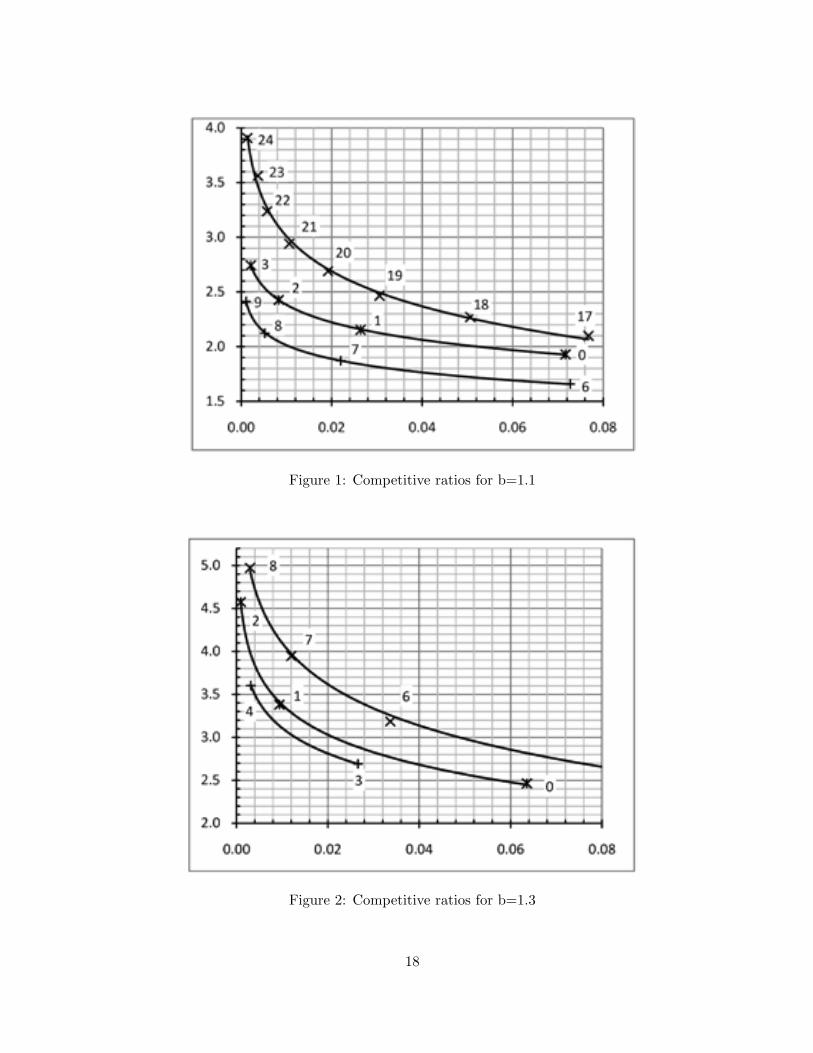
Figure 1: Competitive ratios for b=1.1

Figure 2: Competitive ratios for b=1.3

18

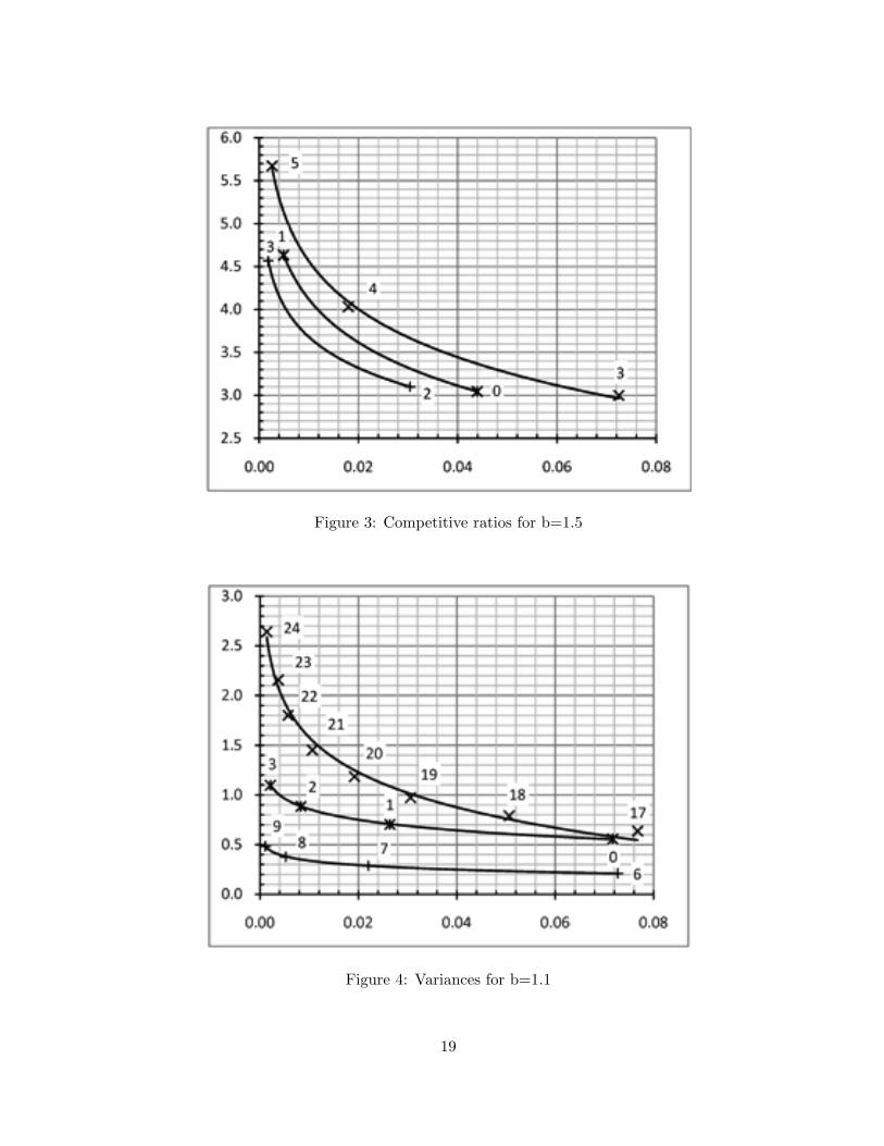
Figure 3: Competitive ratios for b=1.5

Figure 4: Variances for b=1.1

19

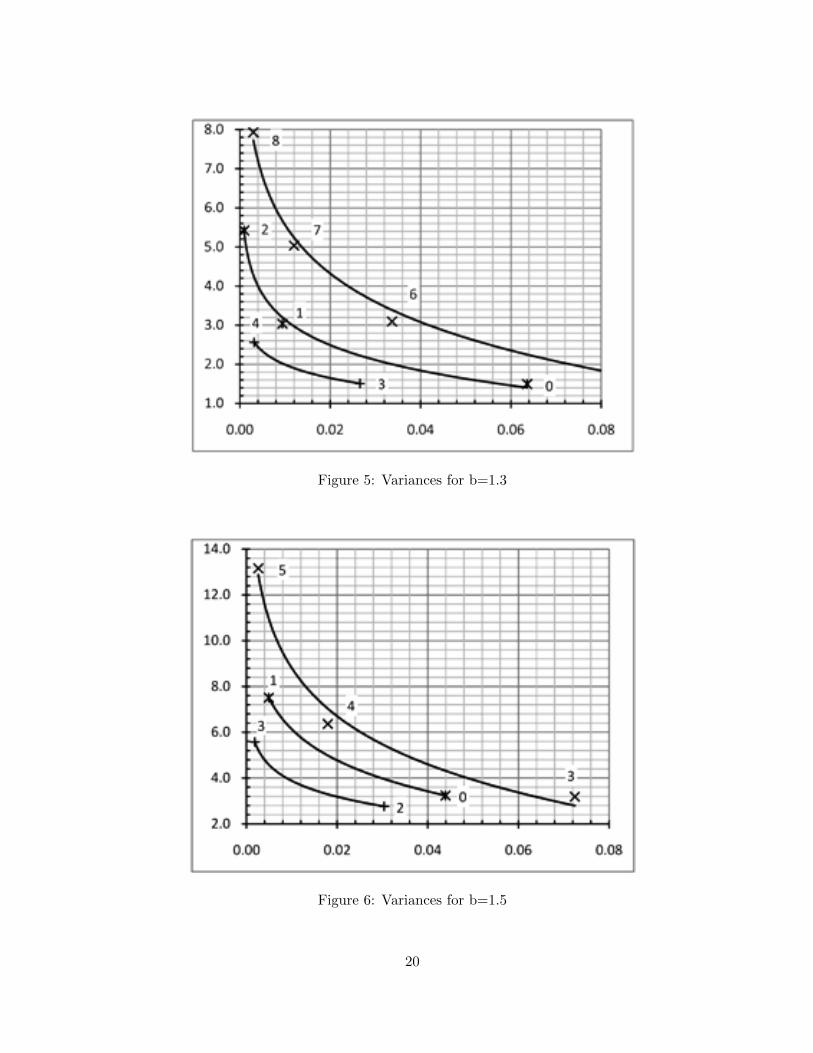
Figure 5: Variances for b=1.3

Figure 6: Variances for b=1.5

20