COMPUTING THE TUTTE POLYNOMIALIN VERTEX-EXPONENTIAL TIME

ANDREAS BJORKLUND∗, THORE HUSFELDT∗, PETTERI KASKI†, AND MIKKO KOIVISTO†

Abstract. The deletion–contraction algorithm is perhaps the most popular method forcomputing a host of fundamental graph invariants such as the chromatic, flow, and reli-ability polynomials in graph theory, the Jones polynomial of an alternating link in knottheory, and the partition functions of the models of Ising, Potts, and Fortuin–Kasteleynin statistical physics. Prior to this work, deletion–contraction was also the fastest knowngeneral-purpose algorithm for these invariants, running in time roughly proportional tothe number of spanning trees in the input graph.

Here, we give a substantially faster algorithm that computes the Tutte polynomial—andhence, all the aforementioned invariants and more—of an arbitrary graph in time within apolynomial factor of the number of connected vertex sets. The algorithm actually evaluatesa multivariate generalization of the Tutte polynomial by making use of an identity due toFortuin and Kasteleyn. We also provide a polynomial-space variant of the algorithm andgive an analogous result for Chung and Graham’s cover polynomial.

An implementation of the algorithm outperforms deletion–contraction also in practice.

1. Introduction

Tutte’s motivation for studying what he called the “dichromatic polynomial” was algo-rithmic. By his own entertaining account [41], he was intrigued by the variety of graphinvariants that could be computed with the deletion–contraction algorithm, and “playing”with it he discovered a bivariate polynomial that we can define as

(1) TG(x, y) =∑F⊆E

(x− 1)c(F )−c(E)(y − 1)c(F )+|F |−|V | .

Here, G is a graph with vertex set V and edge set E; by c(F ) we denote the number ofconnected components in the graph with vertex set V and edge set F . Later, Oxley andWelsh [36] showed in their celebrated Recipe Theorem that, in a very strong sense, theTutte polynomial TG is indeed the most general graph invariant that can be computed usingdeletion–contraction.

Since the 1980s it has become clear that this construction has deep connections to manyfields outside of computer science and algebraic graph theory. It appears in various guisesand specialisations in enumerative combinatorics, statistical physics, knot theory and net-work theory. It subsumes the chromatic, flow, and reliability polynomials, the Jones polyno-mial of an alternating link, and, perhaps most importantly, the models of Ising, Potts, andFortuin–Kasteleyn, which appear in tens of thousands of research papers. A number of sur-veys written for various audiences present and explain these specialisations [39, 43, 44, 45].

∗Lund University, Department of Computer Science, P.O.Box 118, SE-22100 Lund, Sweden. E-mail:andreas.bjorklund@logipard.com, thore.husfeldt@cs.lu.se.†Helsinki Institute for Information Technology HIIT, Department of Computer Science, University of

Helsinki, P.O.Box 68, FI-00014 University of Helsinki, Finland. E-mail: petteri.kaski@cs.helsinki.fi,mikko.koivisto@cs.helsinki.fi. This research was supported in part by the Academy of Finland, Grants117499 (P.K.) and 109101 (M.K.).

1

arX

iv:0

711.

2585

v4 [

cs.D

S] 1

4 A

pr 2

008

2

Computing the Tutte polynomial has been a very fruitful topic in theoretical computerscience, resulting in seminal work on the computational complexity of counting, severalalgorithmic breakthroughs both classical and quantum, and whole research programmesdevoted to the existence and nonexistence of approximation algorithms. Its specialisationto graph colouring has been one of the main benchmarks of progress in exact algorithms.

The deletion–contraction algorithm computes TG for a connected G in time within apolynomial factor of τ(G), the number of spanning trees of the graph, and no essentiallyfaster algorithm was known. In this paper we show that the Tutte polynomial—and hence,by virtue of the Recipe Theorem, every graph invariant admitting a deletion–contractionrecursion—can be computed in time within a polynomial factor of σ(G), the number ofvertex subsets that induce a connected subgraph. Especially, the algorithm runs in timeexp(O(n)

), that is, in “vertex-exponential” time, while τ(G) typically is exp

(ω(n)

)and

can be as large as nn−2 [12]. Previously, vertex-exponential running time bounds wereknown only for evaluations of TG in special regions of the Tutte plane (x, y), such as forthe chromatic polynomial and (using exponential space) the reliability polynomial, or onlyfor special classes of graphs such as planar graphs or bounded-degree graphs. We providea more detailed overview of such prior work in §2.

1.1. Result and consequences. By “computing the Tutte polynomial” we mean com-puting the coefficients tij of the monomials xiyj in TG(x, y) for a graph G given as input.Of course, the coefficients also enable the efficient evaluation of TG(x, y) at any given point(x, y). Our main result is as follows.

Theorem 1. The Tutte polynomial of an n-vertex graph G can be computed(a) in time and space σ(G)nO(1);(b) in time 3nnO(1) and polynomial space; and(c) in time 3n−s2snO(1) and space 2snO(1) for any integer s, 0 ≤ s ≤ n.

Especially, the Tutte polynomial can be evaluated everywhere in vertex-exponential time.In some sense, this is both surprising and optimal, a claim that we solidify under theExponential Time Hypothesis in §2.5. Moreover, even for those curves and points of theTutte plane where a vertex-exponential time algorithm was known before, our algorithmimproves or at least matches their performance, with only a few exceptions (see Figure 1).

For bounded-degree graphs G, the deletion–contraction algorithm itself runs in vertex-exponential time because τ(G) = exp

(O(n)

). Theorem 1 still gives a better bound because

it is known that σ(G) = O((2 − ε)n) for bounded degree [7, Lemma 6], while τ(G) growsfaster than 2.3n already for 3-regular graphs (see §2.4). The precise bound is as follows:

Corollary 2. The Tutte polynomial of an n-vertex graph with maximum vertex degree ∆can be computed in time ξn∆n

O(1), where ξ∆ = (2∆+1 − 1)1/(∆+1).

The question about solving deletion–contraction based algorithmic problems in vertex-exponential time makes sense in directed graphs as well. Here, the most successful attemptto define an analogue of the Tutte polynomial is Chung and Graham’s cover polynomial,which satisfies directed analogues to the deletion–contraction operations [13]. It turns outthat a directed variant of our main theorem can be established using recent techniques thatare by now well understood, we include the precise statement and proof in Appendix C.

1.2. Overview of techniques. The Tutte polynomial is, in essence, a sum over connectedspanning subgraphs. Managing this connectedness property introduces a computational

3

1

2

2

x

y

x=

1‘r

elia

bilit

y’:

3nn

O(1

)

x=

0‘fl

ow’

y = 0 ‘chromatic’: 2nnO(1)

(x− 1)(y − 1) = 1: nO(1)

(x− 1)(y − 1) = 2 ‘Ising’: 2nnO(1)

(x− 1)(y − 1) = q ‘q-state Potts’: qnnO(1)

spanning treesspanning forests: 2nnO(1)

acyclic orientations

connected spanning subgraphs

xy = 1 ‘Jones’

...3-

colo

urin

gs:O

(1.6

262n

)

4-co

lour

ings

:O

(1.9

464n

)

bipa

rtit

ions

dimension of bicycle space

Eulerian

empty

Figure 1. An atlas of the Tutte plane (x, y). The five points shown bycircles and the points on the hyperbola (x − 1)(y − 1) = 1 are in P, allother points are #P-complete. Those points and lines where algorithms withcomplexity exp

(O(n)

)were previously known (sometimes only in exponential

space), are labelled with their running time; note that the hyperbolas (x −1)(y−1) = q were known to be vertex-exponential only for fixed integer q. See§2.3 for references. Our result is that the entire plane admits algorithms withrunning time 2nnO(1) and exponential space, or time 3nnO(1) and polynomialspace. The only points that are known to admit algorithms with betterbounds are the “colouring” points (−2, 0) and (−3, 0), the “Ising” hyperbola(x − 1)(y − 1) = 2, for which a faster algorithm in observed in §2.3, and ofcourse the points in P. (Only the positive branches of the hyperbolas aredrawn.)

challenge not present with its specialisations, e.g., with the chromatic polynomial. Neitherthe dynamic programming algorithm across vertex subsets by Lawler [34] nor the recentinclusion–exclusion algorithm [8], which apply for counting k-colourings, seems to workdirectly for the Tutte polynomial. Perhaps surprisingly, they do work for the cover polyno-mial, even though the application is quite involved; the details are in Appendix C and canbe seen as an attempt to explain just how far these concepts get us.

For the Tutte polynomial, we take a detour via the Potts model. The idea is to eval-uate the partition function of the q-states Potts model at suitable points using inclusion–exclusion, which then, by a neat identity due to Fortuin and Kasteleyn [16, 39], enablesthe evaluation of the Tutte polynomial at any given point by polynomial interpolation. Fi-nally, another round of polynomial interpolation yields the desired coefficients of the Tuttepolynomial. Each step can be implemented using only polynomial space. Moreover, theapproach readily extends to the multivariate Tutte polynomial of Sokal [39] which allows

4

the incorporation of arbitrary edge weights; that generalisation can be communicated quiteconcisely using the involved high-level framework, which we do in §3. To finally arrive atthe main result of this paper—reducing the running time to within a polynomial factorof σ(G)—requires manipulation at the level of the fast Moebius transform “inside” the al-gorithm, which can be found in §4.1. The smooth time–space tradeoff, Theorem 1(c), isobtained by a new “split transform” technique (Appendix B).

Our approach highlights the algorithmic significance of the Fortuin–Kasteleyn identity,and suggests a more general technique: to compute a polynomial, it may be advisable to lookat its evaluations at integral (or otherwise special) points, with the objective of obtainingnew combinatorial or algebraic interpretations that then enable faster reconstruction of theentire polynomial. (For example, the multiplication of polynomials via the fast Fouriertransform can be seen as an instantiation of this technique.)

We also give another vertex-exponential time algorithm that does not rely on interpola-tion (§4.2). It is based on a new recurrence formula that alternates between partitioning aninduced subgraph into components and a subtraction step to solve the connected case. Therecurrence can be solved using fast subset convolution [6] over a multivariate polynomialring. However, an exponential space requirement seems inherent to that algorithm.1 Ap-pendix D briefly reports on our experiences with implementing and running this algorithm;it outperforms deletion–contraction in the worst case when n ≥ 13.

1.3. Conventions. For standard graph-theoretic terminology we refer to West [46]. Allgraphs we consider are undirected and may contain multiple edges and loops. For a graphG, we write n = n(G) for the number of vertices, m = m(G) for the number of edges,V = V (G) for the vertex set, E = E(G) for the edge set, c = c(G) for the number ofconnected components, τ(G) for the number of spanning trees, and σ(G) the number ofconnected sets, i.e., the number of vertex subsets that induce a connected graph.

To simplify running time bounds, we assume m = nO(1) and remark that this assumptionis implicit already in Theorem 1. (Without this assumption, all the time bounds require anadditional multiplicative term mO(1).) For a set of vertices U ⊆ V (G), we write G[U ] forthe subgraph induced by U in G. A subgraph H of G is spanning if V (H) = V (G). For aproposition P , we use Iverson’s bracket notation [P ] to mean 1 if P is true and 0 otherwise.

2. Prior work: Algorithms for the Tutte Polynomial

The direct evaluation of TG(x, y) based on (1) takes 2mnO(1) steps and polynomial space,but many other expansions have been studied in the literature.

2.1. Spanning Tree Expansion. If we expand and collect terms in (1) we arrive at

(2) TG(x, y) =∑i,j

tijxiyj .

In fact, this is Tutte’s original definition. The coefficients tij of this expansion are well-studied: assuming that G is connected, tij is the number of spanning trees of G having“internal activity” i and “external activity” j. What these concepts mean need not occupyus here (for example, see [4, §13]), for our purposes it is sufficient to know that they canbe efficiently computed for a given spanning tree. Thus (2) can be evaluated directly byiterating over all spanning trees of G, which can be accomplished with polynomial delay[27]. The resulting running time is within a polynomial factor of τ(G).

1A previous version of this manuscript followed this route, establishing Theorem 1(a).

5

Some of the coefficients tij have an alternative combinatorial interpretation, and somecan be computed faster than others. For example, t00 = 0 holds if m > 0, and t01 = t10

if m > 1. The latter value, the chromatic invariant θ(G), can be computed from thechromatic polynomial, and thus can be found in time 2nnO(1) [8].

The computational complexity of computing individual coefficients tij has also been in-vestigated. In particular, polynomial-time algorithms exist for tn−1−k,j for constant k andall j = 0, 1, . . . ,m− n+ 1. In general, the task of computing tij is #P-complete [2].

2.2. Deletion–Contraction. The classical algorithm for computing TG is the followingdeletion–contraction algorithm. It is based on two graph transformations involving an edgee. The graph G\e is obtained from G by deleting e. The graph G/e is obtained from G bycontracting e, that is, by identifying the endvertices of e and then deleting e.

With these operations, one can establish the recurrence formula

(3) TG(x, y) =

1 if G has no edges;yTG\e(x, y) if e is a loop;xTG/e(x, y) if e is a bridge;TG\e(x, y) + TG/e(x, y) otherwise.

The deletion–contraction algorithm defined by a direct evaluation of (3) leads to a runningtime that scales as the Fibonacci sequence,

((1 +

√5)/2

)n+m = O(1.6180n+m) [47]. Sekine,Imai, and Tani [38] observed that the corresponding computation tree has one leaf for everyspanning tree of G, so (3) is yet another way to evaluate TG in time within a polynomialfactor of τ(G). In practice one can speed up the computation by identifying isomorphicgraphs and using dynamic programming to avoid redundant recomputation [22, 24, 38].

The deletion–contraction algorithm is known to compute many different graph parame-ters. For example, the number of spanning trees admits an analogous recursion, as does thenumber of acyclic orientations, the number of colourings, the dimension of the bicycle space,and so forth [20, §15.6–8]. This is no surprise: all these graph parameters are evaluations ofthe Tutte polynomial at certain points. But not only is every specialisation of TG express-ible by deletion–contraction, the converse holds as well: every graph parameter that can beexpressed as a deletion–contraction recursion turns out to be a valuation of TG, accordingto the celebrated Recipe Theorem of Oxley and Welsh [36] (cf. [10, Theorem X.2]).

Besides deletion–contraction, many other expansions are known (in particular for restric-tions of the Tutte polynomial; see [4]), even a convolution over the set of edges [33], butnone leads to vertex-exponential time.

2.3. Regions of the Tutte plane. The question at which points (x, y) the Tutte poly-nomial can be computed exactly and efficiently was completely settled in the framework ofcomputational complexity in the seminal paper of Jeager, Vertigan, and Welsh [26]: Theypresented a complete classification of points and curves where the problem is polynomial-time computable, and where it is #P-complete. This result shows us where we probablyneed to resign ourselves to a superpolynomial-time algorithm.

For most of the #P-hard points, the algorithms from §2.1 and §2.2 were best known.However, for certain regions of the Tutte plane, algorithms running in time exp

(O(n)

)have been known before. We attempt to summarise these algorithms here, including thepolynomial-time cases; see Figure 1.

6

Trivial hyperbola: On the hyperbola (x − 1)(y − 1) = 1 the terms of (1) involvingc(F ) cancel, so TG(x, y) = (x−1)n−cym, which can be evaluated in polynomial time.

Ising model: On the hyperbola H2 ≡ (x− 1)(y− 1) = 2, the Tutte polynomial givesthe partition function of the Ising model, a sum of easily computable weights overthe 2n configurations of n two-state spins. This can be trivially computed in time2nnO(1) and polynomial space. By dividing the n spins into three groups of aboutequal size and using fast matrix multiplication, one can compute the sum in time2nω/3nO(1) = O(1.732n) and exponential space, where ω is the exponent of matrixmultiplication; this is yet a new application of Williams’s trick [5, 32, 48].

Potts model: More generally, for any integer q ≥ 2, the Tutte polynomial on thehyperbola Hq ≡ (x − 1)(y − 1) = q gives the partition function of the q-statePotts model [37]. This is a sum over the configurations of n spins each having q

possible states. It can be computed trivially in time qnnO(1) and, via fast matrixmultiplication, in time qn3/ωnO(1). We will show in §3 that, in fact, time 2nnO(1)

suffices, which result will be an essential building block in our main construction.Reliability polynomial: The reliability polynomial RG(p), which is the probability

that no component of G is disconnected after independently removing each edgewith probability 1 − p, satisfies RG(p) = pm−n+c(1 − p)n−cTG(1, 1/p) and can beevaluated in time 3nnO(1) and exponential space [11].

Number of spanning trees: For connected G, TG(1, 1) equals the number τ(G) ofspanning trees, and is computable in polynomial time as the determinant of a maxi-mal principal submatrix of the Laplacian of G, a result known as Kirchhoff’s Matrix–Tree Theorem.

Number of spanning forests: The number of spanning forests, TG(2, 1), is com-putable in time 2nnO(1) by first using the Matrix–Tree Theorem for each inducedsubgraph and then assembling the result one component (that is, tree) at a time viainclusion–exclusion [8]. (This observation is new to the present work, however.)

Dimension of the bicycle space: TG(−1,−1) computes the dimension of the bicy-cle space, in polynomial time by Gaussian elimination.

Number of nowhere-zero 2-flows: TG(0,−1) = 1 if G is Eulerian (in other words,it “admits a nowhere-zero 2-flow”), and TG(0,−1) = 0 otherwise. Thus TG(0,−1)is computable in polynomial time.

Chromatic polynomial: The chromatic polynomial PG(t), which counts the numberof proper t-colourings of the vertices of G, satisfies PG(t) = (−1)n−ctcTG(1 − t, 0)and can be computed in time 2nnO(1) [8]. Vertex-exponential time algorithms wereknown at least since Lawler [34], and a vertex-exponential, polynomial-space algo-rithm was found only recently [5]. Other approaches to the chromatic polynomialare surveyed by Anthony [3]. At t = 2 (equivalently, x = −1) this is polynomial-time computable by breadth-first search (every connected component of a bipartitegraph has exactly two proper 2-colourings). The cases t = 3, 4 are well-studiedbenchmarks for exact counting algorithms, the current best bounds are O(1.6262n)and O(1.9464n) [15]. The case x = 0 is trivial.

To the best knowledge of the authors, no algorithms with running time exp(O(n)

)have

been known for other real points. If we allow x and y to be complex, there are four morepoints (x, y) at which TG can be evaluated in polynomial time [26].

7

2.4. Restricted graph classes. Explicit formulas for Tutte polynomial have been derivedfor many elementary families of graphs, such as T (Cn;x, y) = y + x + x2 + · · · + xn−1 forthe n-cycle graph Cn. We will not give an overview of these formulas here (see [4, §13]);most of them are applications of deletion–contraction.

For well-known graph classes, the authors know the following results achieving exp(O(n)

)running time or better:

Planar graphs: If G is planar, then the Tutte polynomial can be computed in timeexp(O(√n ))

[38]. This works more generally, with a slight overhead: in classes ofgraphs with separators of size nα, the Tutte polynomial can be computed in timeexp(O(nα log n)

).

Bounded tree-width and branch-width: For k a fixed integer, if G has tree-widthk then TG can be computed in polynomial time [1, 35]. This can be generalised tobranch-width [23].

Bounded clique-width and cographs: For k a fixed integer, if G has clique-widthk then TG can be computed in time exp

(O(n1−1/(k+2))

)[18]. A special case of this

is the class of cographs (graphs without an induced path of 4 vertices), where thebound becomes exp

(O(n2/3)

).

Bounded-degree graphs: If ∆ is the maximum degree of a vertex, the deletion–contraction algorithm and 2m ≤ n∆ yield the vertex-exponential running timebound O

(1.6180(1+∆/2)n

)directly from the recurrence. Gebauer and Okamoto im-

prove this to χn∆nO(1), where χ∆ = 2(1−∆2−∆)1/(∆+1) (for example, χ3 = 2.5149,

χ4 = 3.7764, and χ5 = 5.4989). For k-regular graphs with k ≥ 3 a constantindependent of n, the number of spanning trees (and hence, within a polyno-mial factor, the running time of the deletion–contraction algorithms) is boundedby τ(G) = O

(νnkn

−1 log n), where νk = (k − 1)k−1/(k2 − 2k)k/2−1 (for example,

ν3 = 2.3094, ν4 = 3.375, and ν5 = 4.4066), and this bound is tight [14].Interval graphs: If G is an interval graph, then TG can be computed in timeO(1.9706m), which is not exp

(O(n)

)in general, but still faster than by deletion–

contraction [17].

What we cannot survey here is the extensive literature that studies algorithms thatsimultaneously specialise TG and restrict the graph classes, often with the goal of developinga polynomial-time algorithm. A famous example is that for Pfaffian orientable graphs, whichincludes the class of planar graphs, the Tutte polynomial is polynomial-time computableon the hyperbola H2 [29]. Within computer science, the most studied specialisation of thistype is most likely graph colouring for restricted graph classes.

2.5. Computional complexity. The study of the computational complexity of the Tuttepolynomial begins with Valiant’s theory of #P-completeness [42] and the exact complexityresults of Jaeger, Vertigan, and Welsh [26]. The study of the approximability of the valuesof TG has been a very fruitful research direction, an overview of which is again outside thescope of this paper. In this regard we refer to Welsh’s monograph [43] and to the recentpaper of Goldberg and Jerrum [21] for a survey of newer developments.

For our purposes, the most relevant hardness results have been established under theExponential Time Hypothesis [25] (ETH). First, deciding whether a given graph can be3-coloured requires exp(Ω(n)) time under ETH, and since 3-colourability can be decided

8

by computing TG(−2, 0) we see that evaluating the Tutte polynomial requires vertex-exponential time under ETH. Thus, it would be surprising if our results could be significantlyimproved, for example to something like exp

(O(n/ log n)

).

Second, it is by no means clear that the entire Tutte plane should admit such algorithms.Many specialisations of the Tutte polynomial can be understood as constraint satisfactionproblems. For example, graph colouring is an instance of (q, 2)-CSP, the class of constraintsatisfaction problems with pairwise constraints over q-state variables. Similarly, the par-tition function for the Potts model can be seen as a weighted counting CSP [19]. Veryrecently, Traxler [40] has shown that already the decision version of (q, 2)-CSP requirestime exp

(Ω(n log q)

)under ETH, even for some very innocent-looking restrictions, and

even for bounded degree graphs. Thus in general, these CSPs are not vertex-exponentialunder ETH.

3. The multivariate Tutte polynomial via the q-state Potts model

Let R be a multivariate polynomial ring over a field and let G be an undirected graphwith vertex set V = 1, 2, . . . , n and edge set E, m = nO(1). We allow G to have paralleledges and loops. Associate with each e ∈ E a ring element re ∈ R. The multivariate Tuttepolynomial [39] of G is the polynomial

(4) ZG(q, r) =∑F⊆E

qc(F )∏e∈F

re ,

where q is an indeterminate and c(F ) denotes the number of connected components in thegraph with vertex set V and edge set F . The product over an empty set always evaluatesto 1.

The classical Tutte polynomial TG(x, y) can be recovered as a bivariate evaluation of themultivariate polynomial ZG(q, r) via

(5) TG(x, y) = (x− 1)−c(E)(y − 1)−|V |ZG((x− 1)(y − 1), y − 1

).

3.1. The Fortuin–Kasteleyn identity. At points q = 1, 2, . . . the multivariate Tuttepolynomial ZG(q, r) can be represented as an evaluation of the partition function of theq-state Potts model [16, 39].

For a mapping s : V → 1, 2, . . . , q and an edge e ∈ E with endvertices x and y, defineδse = 1 if s(x) = s(y) and δse = 0 if s(x) 6= s(y). The partition function of the q-state Pottsmodel on G is defined by

(6) ZPottsG (q, r) =

∑s:V→1,2,...,q

∏e∈E

(1 + reδ

se

).

Theorem 3 (Fortuin and Kasteleyn). For all q = 1, 2, . . . it holds that

(7) ZG(q, r) = ZPottsG (q, r) .

3.2. The multivariate Tutte polynomial via the q-state Potts model. By virtue ofthe Fortuin–Kasteleyn identity (7), to compute ZG(q, r) it suffices to evaluate

ZPottsG (1, r), ZPotts

G (2, r), . . . , ZPottsG (n+ 1, r)

and then recover ZG(q, r) via Lagrangian interpolation. For the interpolation to succeed,it is necessary to assume that the coefficient field of R has a large enough characteristic sothat 1, 2, . . . , n have multiplicative inverses.

9

At first sight the evaluation of (6) for a positive integer q appears to require qnnO(1) ringoperations. Fortunately, one can do better. To this end, let us express ZPotts

G (q, r) in a moreconvenient form. For X ⊆ V , denote by G[X] the subgraph of G induced by X, and let

(8) f(X) =∏

e∈E(G[X])

(1 + re) .

For q = 1, 2, . . ., we have

(9) ZPottsG (q, r) =

∑(U1,U2,...,Uq)

f(U1)f(U2) · · · f(Uq) ,

where the sum is over all q-tuples (U1, U2, . . . , Uq) with U1, U2, . . . , Uq ⊆ V such that∪qi=1Ui = V and Uj ∩ Uk 6= ∅ for all 1 ≤ j < k ≤ q.

We now proceed to develop algorithms for evaluating the Potts partition function in theform (9).

3.3. The baseline algorithm. Let f : 2V → R be a function that associates a ring elementf(X) ∈ R with each subset X ⊆ V .

The zeta transform fζ : 2V → R is defined for all Y ⊆ V by fζ(Y ) =∑

X⊆Y f(X). TheMoebius transform fµ : 2V → R is defined for all X ⊆ V by fµ(X) =

∑Y⊆X(−1)|X\Y |f(Y ).

It is a basic fact that the zeta and Moebius transforms are inverses of each other, thatis, fζµ = fµζ = f for all f . Furthermore, it is known [6] that

(10)((fζ)qµ

)(V ) =

∑(U1,U2,...,Uq)

f(U1)f(U2) · · · f(Uq) ,

where the sum is over all q-tuples (U1, U2, . . . , Uq) with U1, U2, . . . , Uq ⊆ V and ∪qj=1Uj = V .In particular,

((fζ)qµ

)(V ) can be computed directly in 3nnO(1) ring operations by storing

nO(1) ring elements. Using the fast zeta and Moebius transforms,((fζ)qµ

)(V ) can be

computed in 2nnO(1) ring operations by storing 2nnO(1) ring elements [6].To use this to evaluate (9), adjoin a new indeterminate z into R to obtain the polynomial

ring R[z]. Replace f with fz : 2V → R[z] defined for all X ⊆ V by fz(X) = f(X)z|X|. Nowevaluate the z-polynomial

((fzζ)qµ

)(V ) and look at the coefficient of the monomial z|V |,

which by virtue of (10) is equal to (9).This baseline algorithm together with (5), (7), and Lagrangian interpolation establishes

that the Tutte polynomial TG(x, y) can be computed (a) in time and space 2nnO(1); and(b) in time 3nnO(1) and space nO(1). This proves Theorem 1(b). A more careful analysis of((fζ)qµ

)(V ) enables the time–space tradeoff in Theorem 1(c). [[ See Appendix B. ]]

4. Improvements and variations

4.1. An algorithm over connected sets. It is useful to think of X ⊆ V in what follows asthe current subset under consideration. We start with a lemma that partitions the subsetsof X based on the maximum common suffix. To this end, let Y≡iX be a shorthand forY ∩ i+ 1, i+ 2, . . . , n = X ∩ i+ 1, i+ 2, . . . , n.

Lemma 4 (Suffix partition). Let Y ⊆ X ⊆ 1, 2, . . . , n. Then, either Y = X or thereexists a unique i ∈ X such that Y≡i−1X \ i.

Proof. Either Y = X or i = maxX \ Y .

10

The intermediate values computed by the algorithm are now defined as follows.

Definition 5. Let X ⊆ V , q = 1, 2, . . . , n+ 1, and i = 0, 1, . . . , n. Let

F (X, q, i) =∑

(U1,U2,...,Uq)

q∏j=1

f(Uj) ,

where the sum is over all q-tuples (U1, U2, . . . , Uq) such that both U1, U2, . . . , Uq ⊆ X and∪qj=1Uj≡iX.

Note that F (V, q, 0) = ((fζ)qµ)(V ). Thus, it suffices to compute F (V, q, 0).We are now ready to describe the algorithm that computes the intermediate values

F (X, q, i) in Definition 5. The algorithm considers one set X ⊆ V at a time, startingwith the empty set X = ∅ and proceeding upwards in the subset lattice. It is required thatthe maximal proper subsets of X have been considered before X itself is considered; forexample, we can consider the subsets of V in increasing lexicographic order. The commentsdelimited by “[[” and “]]” justify the computations in the algorithm.

Algorithm U. (Up-step.) Computes the values F (X, q, i) associated with X using thevalues associated with X \ i for all i ∈ X.Input: A subsetX ⊆ V and the value F (X\i, q, i−1) for each i ∈ X and q = 1, 2, . . . , n+1.Output: The value F (X, q, i) for each q = 1, 2, . . . , n+ 1 and i = 0, 1, . . . , n.

U1: For each q = 1, 2, 3, . . . , n+ 1, set

F (X, q, n) =(f(X) +

∑i∈X

F (X \ i, 1, i− 1))q

.

[[ By the suffix partition lemma,∑

Y(X f(Y ) =∑

i∈X F (X \ i, 1, i− 1). Addingf(X) and taking powers, we obtain F (X, q, n). ]]

U2: For each q = 1, 2, 3, . . . , n+ 1 and i = n, n− 1, . . . , 1, set

F (X, q, i− 1) = F (X, q, i)− [i ∈ X]F (X \ i, q, i− 1) .

[[ There are two cases to consider to justify correctness. First, assume that i /∈ X.Consider an arbitrary q-tuple (U1, U2, . . . , Uq) with U1, U2, . . . , Uq ⊆ X. Let Y =∪qj=1Uj . Clearly, Y ⊆ X. Because i /∈ X and Y ⊆ X, we have Y≡i−1X if andonly if Y≡iX. Thus, F (X, q, i− 1) = F (X, q, i). Second, assume that i ∈ X. Inthis case we have Y≡iX if and only if either Y≡i−1X or Y≡i−1X\i (the formercase occurs if i ∈ Y , the latter if i /∈ Y ). In the latter case, Y ⊆ X \i and henceU1, U2, . . . , Uq ⊆ X \i. Thus, F (X, q, i− 1) = F (X, q, i)−F (X \i, q, i− 1). ]]

Assume that f satisfies the following property: for all X ⊆ V it holds that

(11) f(X) = f(X1)f(X2) · · · f(Xs)

where G[X1], G[X2], . . . , G[Xs] are the connected components of G[X]. For conveniencewe also assume that f(∅) = 1. Note that the factorisation (11) is well-defined because ofcommutativity of R. Also note that (8) satisfies (11).

Lemma 6. Let G[X1], G[X2], . . . , G[Xs] be the connected components of G[X]. Then,

(12) F (X, q, i) =s∏

k=1

F (Xk, q, i) .

11

The recursion (12) now enables the following top-down evaluation strategy for the inter-mediate values in Definition 5. Consider a nonempty X ⊆ V . If G[X] is not connected,recursively solve the intermediate values of each of the vertex sets X1, X2, . . . , Xs of theconnected components G[X1], G[X2], . . . , G[Xs] of G[X], and assemble the solution using(12). Otherwise; that is, if G[X] is connected, recursively solve the intermediate values ofeach set X \ i, i ∈ X, and assemble the solution using Algorithm U. Call this evaluationstrategy Algorithm C.

Algorithm C together with (5), (7), and Lagrangian interpolation establishes that theTutte polynomial TG(x, y) can be computed in time and space σ(G)nO(1). This provesTheorem 1(a).

4.2. An alternative recursion. We derive an alternative recursion for ZG(q, r) based oninduced subgraphs and fast subset convolution. Let R be a commutative ring. Associate aring element re ∈ R with each e ∈ E. For k = 1, 2, . . . , n, let

SG(k, r) =∑F⊆Ec(F )=k

∏e∈F

re

and observe that ZG(q, r) =∑n

k=1 qkSG(k, r). Thus, to determine ZG(q, r), it suffices to

compute SG(k, r) for all k = 1, 2, . . . , n.To this end, the values SG(k, r) can be computed using the following recursion over

induced subgraphs of G. Let W ⊆ V and consider the subgraph G[W ] induced by W in G.Suppose that SG[U ](k, r) has been computed for all ∅ 6= U ( W and k = 1, 2, . . . , |U |.

To compute SG[W ](k, r) for k = 2, 3, . . . , |W |, observe that a disconnected subgraph ofG[W ] partitions into connected components. Thus, for k ≥ 2 we have

(13) SG[W ](k, r) =1k

∑∅6=U(W

SG[U ](1, r)SG[W\U ](k − 1, r) .

For the connected case, that is, for k = 1, it suffices to observe that we can subtract thedisconnected subgraphs from the set of all subgraphs to obtain the connected graphs; putotherwise,

(14) SG[W ](1, r) =∏

e∈E(G[W ])

(1 + re)−∑k≥2

SG[W ](k, r) .

The recursion defined by (13) and (14) can now be evaluated for |W | = 1, 2, . . . , n intotal 2nnO(1) ring operations using fast subset convolution [6]. As a technical observationwe remark that (13) assumes that k has a multiplicative inverse in R; this assumptioncan be removed, but we omit the details from this extended abstract. We also note thatanalogues of Algorithms U and C running in σ(G)nO(1) ring operations can be developedin this context; we describe an implementation of this in Appendix D. However, it is notimmediate whether a polynomial-space algorithm for the Tutte polynomial can be developedbased on (13) and (14).

References p. 1

References

[1] A. Andrzejak, An algorithm for the Tutte polynomials of graphs of bounded treewidth, Discrete Math.190 (1998), 39–54.

[2] J. D. Annan, The complexities of the coefficients of the Tutte polynomial, Discrete Appl. Math. 57(1995), 93–103.

[3] M. H. G. Anthony, Computing chromatic polynomials, Ars Combinatoria 29 (1990), 216–220.[4] N. Biggs, Algebraic Graph Theory, 2nd ed., Cambridge University Press, 1993.[5] A. Bjorklund, T. Husfeldt, Exact algorithms for exact satisfiability and number of perfect matchings,

Algorithmica, 2007, doi:10.1007/s00453-007-9149-8.[6] A. Bjorklund, T. Husfeldt, P. Kaski, M. Koivisto, Fourier meets Mobius: fast subset convolution,

Proceedings of the 39th Annual ACM Symposium on Theory of Computing (San Diego, CA, June11–13, 2007), Association for Computing Machinery, 2007, pp. 67–74.

[7] A. Bjorklund, T. Husfeldt, P. Kaski, M. Koivisto, The Travelling Salesman Problem in bounded degreegraphs, Proceedings of the 35th International Colloquium on Automata, Languages and Programming(Reykjavik, Iceland, July 6–13, 2008), to appear.

[8] A. Bjorklund, T. Husfeldt, M. Koivisto, Set partitioning via inclusion–exclusion, SIAM J. Computing,to appear.

[9] M. Blaser, H. Dell, Complexity of the cover polynomial, Proceedings of the 34th International Collo-quium on Automata, Languages and Programming (Wroclaw, Poland, July 9-13, 2007), Lecture Notesin Computer Science 4596, 2007, pp. 801-812.

[10] B. Bollobas, Modern Graph Theory, Graduate Texts in Mathematics 184, Springer, 1998.[11] J. A. Buzacott, A recursive algorithm for finding reliability measures related to the connection of nodes

in a graph, Networks 10 (1980), 311–327.[12] A. Cayley, A theorem on trees, Quart. J. Math. 23 (1889), 376–378.[13] F. R. K. Chung, R. L. Graham, On the cover polynomial of a digraph, J. Combin. Theory Ser. B 65

(1995), 273–290.[14] F. Chung, S.-T. Yau, Coverings, heat kernels, and spanning trees, Electron. J. Combinatorics 6 (1999)

#R12, 21 pp.[15] F. V. Fomin, S. Gaspers, S. Saurabh, Improved exact algorithms for counting 3- and 4-colorings,

Computing and Combinatorics, 13th Annual International Conference (COCOON), Banff, Canada,July 16–19, 2007, Lecture Notes in Computer Science 4598, Springer, 2007, pp. 65–74.

[16] C. M. Fortuin, P. W. Kasteleyn, On the random-cluster model. I. Introduction and relation to othermodels, Physica 57 (1972), 536–564.

[17] H. Gebauer, Y. Okamoto, Fast exponential-time algorithms for the forest counting in graph classes,Theory of Computing 2007, Proceedings of the 13th Computing: The Australasian Theory Sympo-sium (CATS 2007), Ballarat, Victoria, Jan 30–Feb 2, 2007, Conferences in Research and Practice inInformation Technology 65, Australian Computer Society, 2007, pp. 63–69.

[18] O. Gimenez, P. Hlineny, M. Noy, Computing the Tutte polynomial on graphs of bounded clique-width,SIAM J. Discrete Math. 20 (2006), 932–946.

[19] M. Dyer, L.A. Goldberg, and M. Jerrum, The complexity of weighted Boolean #CSP,arXiv:0704.3683v1 [cs.CC] (Apr, 2007).

[20] C. Godsil, G. Royle, Algebraic Graph Theory, Graduate Texts in Mathematics 207, Springer, 2001.[21] L. A. Goldberg, M. Jerrum, Inapproximability of the Tutte polynomial, Proceedings of the 39th An-

nual ACM Symposium on Theory of Computing (San Diego, CA, June 11–13, 2007), Association forComputing Machinery, 2007, pp. 459–468.

[22] G. Haggard, D. Pearce, G. Royle, Computing Tutte polynomials, Technical Report, Victoria Universityof Wellington, NZ, in preparation.

[23] P. Hlineny, The Tutte polynomial for matroids of bounded branch-width, Combin. Probab. Comput.15 (2006), 397–409.

[24] H. Imai, Computing the invariant polynomials of graphs, networks, and matroids, IEICE T. Inf. Syst.E93–D (2000), 330–343.

[25] R. Impagliazzo, R. Paturi, and F. Zane, Which problems have strongly exponential complexity?, J.Comput. Syst. Sci. 63 (2001), 512–530.

[26] F. Jaeger, D. L. Vertigan, D. J. A. Welsh, On the computational complexity of the Jones and Tuttepolynomials, Math. Proc. Cambridge Philos. Soc. 108 (1990), 35–53.

References p. 2

[27] S. Kapoor, H. Ramesh, Algorithms for enumerating all spanning trees of undirected and weightedgraphs, SIAM J. Comput. 24 (1995), 247–265.

[28] R. M. Karp, Dynamic programming meets the principle of inclusion and exclusion, Oper. Res. Lett. 1(1982), 49–51.

[29] P. W. Kasteleyn, The statistics of dimers on a lattice: I. The number of dimer arrangements on aquadratic lattice, Physica 27 (1961), 1209–1225.

[30] D. E. Knuth, The Stanford GraphBase: A Platform for Combinatorial Computing, Association forComputing Machinery, 1993.

[31] S. Kohn, A. Gottlieb, M. Kohn, A generating function approach to the traveling salesman problem,Proceedings of the 1977 Annual Conference (ACM’77), Association for Computing Machinery, 1977,pp. 294–300.

[32] M. Koivisto, Optimal 2-constraint satisfaction via sum-product algorithms, Inform. Process. Lett. 98(2006), 22–24.

[33] W. Kook, V. Reiner, D. Stanton, A convolution formula for the Tutte polynomial, J. Combin. TheorySer. B 76 (1999), 297–300.

[34] E. L. Lawler, A note on the complexity of the chromatic number problem, Inf. Process. Lett. 5 (1976),66–67.

[35] S. D. Noble, Evaluating the Tutte polynomial for graphs of bounded tree-width, Combin. Probab. Com-put. 7 (1998), 307–321.

[36] J. G. Oxley, D. J. A. Welsh, The Tutte polynomial and percolation, Graph Theory and Related Topics(J. A. Bondy and U. S. R. Murty, Eds.), Academic Press, 1979, pp. 329–339.

[37] R. B. Potts, Some generalized order-disorder transformations, Proceedings of the Cambridge Philo-sophical Society 48 (1952), 106–109.

[38] K. Sekine, H. Imai, S. Tani, Computing the Tutte polynomial of a graph of moderate size, Algorithmsand Computation, 6th International Symposium (ISAAC ’95), Cairns, Australia, December 4–6, 1995,Lecture Notes in Computer Science 1004, Springer, 1995, pp. 224–233.

[39] A. D. Sokal, The multivariate Tutte polynomial (alias Potts model) for graphs and matroids, Surveysin Combinatorics, 2005, London Mathematical Society Lecture Note Series 327, Cambridge UniversityPress, 2005, pp. 173–226.

[40] P. Traxler, The Time Complexity of Constraint Satisfaction, Proceedings of the 3rd InternationalWorkshop on Exact and Parameterized Computation (Victoria (BC), Canada, May 14–16, 2008), toappear.

[41] W. T. Tutte, Graph-polynomials, Adv. Appl. Math. 32 (2004), 5–9.[42] L. G. Valiant, The complexity of enumeration and reliability problems, SIAM J. Comput. 8 (1979),

410–421.[43] D. J. A. Welsh, Complexity: Knots, Colourings and Counting, London Mathematical Society Lecture

Note Series 186, Cambridge University Press, 1993.[44] D. J. A. Welsh, The Tutte polynomial, Random Structures Algorithms 15 (1999), 210–228.[45] D. J. A. Welsh, C. Merino, The Potts model and the Tutte polynomial, J. Math. Phys. 41 (2000),

1127–1152.[46] D. B. West, Introduction to Graph Theory, 2nd ed., Prentice–Hall, 2001.[47] H. S. Wilf, Algorithms and Complexity, Prentice–Hall, 1986.[48] R. Williams, A new algorithm for optimal constraint satisfaction and its implications, Theoret. Com-

put. Sci. 348 (2005), 357–365.

Appendix p. 1

Appendix

Appendix A. Proofs

A.1. Proof of Theorem 3. This proof of the Fortuin–Kasteleyn identity (7) is well known(e.g. [39]) and is here included only for convenience of verification.

Proof. Expanding the product over E and changing the order of summation,

ZPottsG (q, r) =

∑s:V→1,2,...,q

∏e∈E

(1 + reδ

se

)=∑F⊆E

∑s:V→1,2,...,q

∏e∈F

reδse .

The right-hand side product evaluates to zero unless s is constant on each connected com-ponent of the graph with vertex set V and edge set F . Because there are q choices for thevalue of s on each connected component,∑

F⊆E

∑s:V→1,2,...,q

∏e∈F

reδse =

∑F⊆E

qc(F )∏e∈F

re = ZG(q, r) .

A.2. Proof of Lemma 6. It is convenient to start with a preliminary lemma.

Lemma 7. Let G[X1], G[X2], . . . , G[Xs] be the connected components of G[X] and let U ⊆X. Then,

f(U) = f(U ∩X1)f(U ∩X2) · · · f(U ∩Xs) .

Proof. Let G[U1], G[U2], . . . , G[Ut] be the connected components of G[U ]. Then, by (11),

f(U) = f(U1)f(U2) · · · f(Ut) .

Because U ⊆ X holds, for every Ui there is a unique h(i) ∈ 1, 2, . . . , s such that Ui ⊆ Xh(i).Moreover, since U1, U2, . . . , Ut is a partition of U , we have that Ui : i ∈ h−1(j) is apartition of U∩Xj for all j = 1, 2, . . . , s. Thus, by (11) we have f(U∩Xj) =

∏i∈h−1(j) f(Ui)

for all j = 1, 2, . . . , s. In particular, by commutativity of R,

f(U) =t∏i=1

f(Ui) =s∏j=1

∏i∈h−1(j)

f(Ui) =s∏j=1

f(U ∩Xj) .

We now proceed with the proof of Lemma 6.

Proof. Consider an arbitrary q-tuple (U1, U2, . . . , Uq) with U1, U2, . . . , Uq ⊆ X and ∪qj=1Uj≡iX.Because X1, X2, . . . , Xs is a partition of X, we have ∪qj=1Uj≡iX if and only if Xk ∩∪qj=1Uj≡iXk ∩X holds for all k = 1, 2, . . . , s. Put otherwise, we have ∪qj=1Uj≡iX if andonly if ∪qj=1(Xk ∩Uj)≡iXk holds for all k = 1, 2, . . . , s. Using Lemma 7 for each Uj in turn,we have, by commutativity of R, the unique factorisation into pairwise intersections

f(U1)f(U2) . . . f(Uq) =q∏j=1

s∏k=1

f(Uj ∩Xk) =s∏

k=1

q∏j=1

f(Uj ∩Xk) .

The claim follows because (U1, U2, . . . , Uq) was arbitrary.

Appendix p. 2

Appendix B. A time–space tradeoff via split transforms

This appendix outlines a “split transform” algorithm that enables a time–space tradeoffin evaluating

((fζ)qµ

)(V ) for a given function f : 2V → R and q = 1, 2, . . . , n+ 1.

Split the ground set V = 1, 2, . . . , n into two parts, V1 ⊆ V and V2 ⊆ V , such thatV = V1 ∪ V2 and V1 ∩ V2 = ∅. Let n1 = |V1| and n2 = |V2|. For a subset X ⊆ V , we usesubscripts to indicate the parts of the subset in V1 and V2; that is, we let X1 = X ∩ V1 andX2 = X ∩ V2. It is also convenient to split the function notation accordingly, that is, wewrite f(X1, X2) for f(X1∪X2) = f(X). In the context of zeta and Moebius transforms, weuse X for a subset in the “spatial” (original) domain and Y for a subset in the “frequency”(transformed) domain.

An elementary observation is now that both the zeta and Moebius transforms split, thatis,

fζ(Y ) =∑X⊆Y

f(X) =∑X1⊆Y1

∑X2⊆Y2

f(X1, X2) =∑X1⊆Y1

fζ2(X1, Y2) = fζ2ζ1(Y1, Y2)

and

fµ(X) =∑Y⊆X

(−1)|X\Y |f(Y ) =∑X1⊆Y1

(−1)|X1\Y1|∑X2⊆Y2

(−1)|X2\Y2|f(Y1, Y2)

=∑X1⊆Y1

(−1)|X1\Y1|fµ2(Y1, X2) = fµ2µ1(X1, X2) .

Also note that fζ = fζ2ζ1 = fζ1ζ2 and fµ = fµ2µ1 = fµ1µ2.To arrive at the split transform algorithm for computing

((fζ)qµ

)(V ), split the outer

Moebius transform and the inner zeta transform to get((fζ)qµ

)(V ) =

∑Y1⊆V1

(−1)|V1\Y1|∑Y2⊆V2

(−1)|V2\Y2|(fζ1ζ2(Y1, Y2))q .

Now let Y1 be fixed and consider the inner sum. To evaluate the inner sum for a fixed Y1,it suffices to have fζ1ζ2(Y1, Y2) available for each Y2 ⊆ V2. By definition,

fζ1ζ2(Y1, Y2) =∑X2⊆Y2

fζ1(Y1, X2) .

Observe that if we have fζ1(Y1, X2) stored for each X2 ⊆ V2, then we can evaluatefζ1ζ2(Y1, Y2) for each Y2 ⊆ V2 simultaneously using the fast zeta transform. This takesin total at most 2n2n2 ring operations and requires one to store at most 2n2n2 ring ele-ments.

For fixed Y1 and X2, we can evaluate and store

fζ1(Y1, X2) =∑X1⊆Y1

f(X1, X2)

by plain summation in at most 2|Y1| ring operations. Thus, for fixed Y1, we can evaluatefζ1(Y1, X2) for each X2 ⊆ V2 in total at most 2|Y1|2n2 ring operations.

Considering each Y1 ⊆ V1 in turn, we can thus evaluate((fζ)qµ

)(V ) by storing at most

2n2n2 ring elements and executing at most

nO(1)∑Y1⊆V1

(2n2n2 + 2|Y1|2n2) = nO(1)(3n1 + 2n1n2)2n2

Appendix p. 3

ring operations. This completes the description and analysis of the split transform algo-rithm.

The split transform algorithm together with (5), (7), and Lagrangian interpolation provesTheorem 1(c).

Appendix C. The cover polynomial

Let D be a digraph with vertex set V = 1, 2, . . . , n. Note that D may have paralleledges and loops. We assume that the number of edges is nO(1). Denote by cD(i, j) thenumber of ways of disjointly covering all the vertices of D with i directed paths and jdirected cycles. The cover polynomial is defined as

CD(x, y) =∑i,j

cD(i, j)xiyj ,

where xi = x(x − 1) · · · (x − i + 1) and x0 = 1. It is known that CD(x, y) is #P-completeto evaluate except at a handful of points (x, y) [9].

In analogy to Theorem 1, we can show that CD can be computed in vertex-exponentialtime:

Theorem 8. The cover polynomial of an n-vertex directed graph can be computed

(a) in time and space 2nnO(1); and(b) in time 3nnO(1) and polynomial space.

The proof involves several inclusion–exclusion-based arguments with different purposesand in a nested fashion, so we first give a high-level overview of the concepts involved. Onereadily observes that the cover polynomial can be expressed as a sum over partitioningsof the vertex set, each vertex subset appropriately weighted, so the inclusion–exclusiontechnique [8] applies. Computing the weights for all possible vertex subsets is again a hardproblem, but the fast Moebius inversion algorithm [7] can be used to compute the necessaryvalues beforehand. This leads to an exponential-space algorithm. Finally, to use inclusion–exclusion to reduce the space to polynomial [28, 31], we apply the mentioned transforms ina nested manner and switch the order of certain involved summations.

We turn to the details of the proof. For X ⊆ V , denote by p(X) the number of spanningdirected paths in D[X], and denote by c(X) the number of spanning directed cycles inD[X]. Define p(∅) = c(∅) = 0. Note that for all x ∈ V we have p(x) = 1 and that c(x)is the number of loops incident with x.

By definition,

cD(i, j) =1i!j!

∑X1,X2,...,Xi,Y1,Y2,...,Yj

p(X1)p(X2) · · · p(Xi) c(Y1)c(Y2) · · · c(Yj) ,

where we sum over all (i+j)-tuples (X1, X2, . . . , Xi, Y1, Y2, . . . , Yj) such that X1, X2, . . . , Xi,Y1, Y2, . . . , Yj is a partition of V .

We next derive an alternative expression using the principle of inclusion and exclusion.To this end, it is convenient to define for every U ⊆ V the polynomials

P (U ; z) =∑X⊆U

p(X)z|X| and C(U ; z) =∑X⊆U

c(X)z|X|

Appendix p. 4

in an indeterminate z; if viewed as set functions, P (U ; z) and C(U ; z) are zeta transformsof the set functions p(X)z|X| and c(X)z|X|, respectively. We can now write

cD(i, j) =1i!j!

∑U⊆V

(−1)|V \U |zn(P (U ; z)iC(U ; z)j

).

It remains to show how to compute the p(X) and c(X) for all X ⊆ V . For S ⊆ V letw(S, s, t, `) denote the number of directed walks of length ` from vertex s to vertex t inD[S]; define w(S, s, t, `) = 0 if s 6∈ S or t 6∈ S. By inclusion–exclusion, again,

p(X) =∑

1≤s≤t≤n

∑S⊆X

(−1)|X\S|w(S, s, t, |X| − 1) .

Similarly,c(X) =

∑S⊆X

(−1)|X\S|w(S, s, s, |X|) , where s = minS .

Observing that w(S, s, t, `) can be computed in time nO(1), we have that cD(i, j) can becomputed in space nO(1) and time 4nnO(1).

To get an algorithm running in 3nnO(1) time and nO(1) space, observe that

P (U ; z) =∑S⊆U

P (U, S; z)

where

P (U, S; z) =∑

1≤s≤t≤n

|U\S|∑k=0

(|U \ S|k

)(−1)kz|S|+kw(S, s, t, |S|+ k − 1)

andC(U ; z) =

∑S⊆U

C(U, S; z)

where

C(U, S; z) =|U\S|∑k=0

(|U \ S|k

)(−1)kz|S|+kw(S, s, s, |S|+ k) , where s = minS .

This establishes part (b) of the theorem.For part (a), we show how to evaluate cD(i, j) in time and space 2nnO(1). Namely, p and

c can be computed in time and space 2nnO(1) via fast Moebius inversion. Given p and c, thepolynomials P and C can be computed in time and space 2nnO(1) via fast zeta transform.And finally, given P and C, the inclusion–exclusion expression of cD(i, j) can be evaluatedin time 2nnO(1).

Appendix D. Tutte polynomials of concrete graphs

D.1. Algorithm implementation. Our implementation of the algorithm described in §4.2uses a number of extra techniques to reduce the polynomial factors in the time and memoryrequirements. In what follows we assume that G is a connected graph.

(1) The coefficients tij of the Tutte polynomial are computed modulo a small integerp; the computation is repeated for sufficiently many different (pairwise coprime)p to enable recovery of the coefficients via the Chinese Remainder Theorem. Thenumber of different p required is determined based on the available word length and

Appendix p. 5

using τ(G) (computed via the Matrix–Tree Theorem) as an upper bound for thecoefficients.

(2) To save a factor of m in memory, instead of direct computation with bivariatepolynomials, we compute with univariate evaluations of the polynomials at z =0, 1, . . . ,m, and finally recover only the necessary bivariate polynomials from theevaluations via Lagrange interpolation.

(3) To save a further factor of n2 in memory, we execute the analogue of Algorithm Ufor subsets X in a specific order, namely in the lexicographic order. This enablesefficient “in-place” computation of the polynomials F (X, k, i) so that, for each X,the polynomials F (X, k, i) need to be stored only for one value of i at the time.Furthermore, we never need all F (X, k, i) for k = 2, 3, . . . , n explicitly, only a linearcombination of them, so we count with this instead; however, we omit the details inthis abstract.

The source code of the algorithm implementation is available by request. The imple-mentation uses the GNU Multiple Precision Arithmetic library 〈http://gmplib.org/〉 forcomputation with large integers. The computed coefficients tij are checked for consistencyby verifying that

∑i,j tij = τ(G) and that

∑i,j 2i+jtij = 2m.

D.2. Performance. The current algorithm implementation uses roughly 2n+1n words ofmemory for an n-vertex graph, which presents a basic obstacle to practical performance. Forexample, the practical limit is at n = 25, assuming 32 GB of main memory and 64-bit words.This makes our polynomial space and time–space tradeoff algorithms from Theorem 1(b,c)interesting also from a practical perspective. At the time of writing, we have implementedthe former, but not yet performed large-scale experiments with it.

In terms of running time, the complete graph Kn presents the worst case for n-vertexinputs for our algorithm. On a 3.66GHz Intel Xeon CPU with 1MB cache, computing theTutte polynomial of K17 takes less than an hour, K18 takes about three hours, and K22

takes 96 hours. In comparison, both deletion–contraction and spanning tree enumerationcease to be practical well below this; for example, τ(K22) = 705429498686404044207947776and τ(K16) = 72057594037927936; a survey of how to compute TG in practice [24] reportsrunning times for the complete graph K14 in hours. The fastest current program to computeTutte polynomials [22] is also based on deletion–contraction with isomorphism rejection, butuses many other ideas as well. It processes K14 and many sparse graphs with far larger nin a few seconds, but also ceases to be practical for some dense graphs with n = 16, seeFigure 2.

Two further remarks are in order. First, for (connected) graphs with a small τ(G),enumeration of spanning trees is faster than our algorithm. Second, graphs with feweredges are faster to solve using our algorithm. For example, a 3-regular graph on 22 verticescan be solved in about five hours.

D.3. Tutte polynomials of some concrete graphs. Even though few readers are likelyto derive any insight from the fact that the coefficient of x2y2 in the Tutte polynomial ofLoupekine’s Second Snark is 991226, we feel it germane to our paper to actually computesome Tutte polynomials. We include tables of the nonzero coefficients tij in the expan-sion (2) for a number of graphs. Among these, the values for the Petersen graph are wellknown [4, §13b] and are included here for verification only. For reference, we present theTutte polynomials of a few other well-known graphs, mostly snarks and cages; however,these graphs are fairly sparse and exhibit symmetries that make them amenable to many of

Appendix p. 6

1

10

100

1 000

10 000

100 000

1 second

1 minute

1 hour

1 day

12 14 16 18Number of vertices n

Run

ning

tim

e(s

econ

ds)

Figure 2. Running times for complements of random 4-regular graphs. Thelines show averages of 5 runs on a 3.66GHz Intel Xeon CPU with 1MB cache.The thin line is our algorithm; the thick line is the algorithm of Haggard,Pearce, and Royle [22].

the previously existing techniques. An entertaining example that tests the liminations of ourcurrent implementation is from Knuth’s Stanford Graph Base [30], based on the encountersbetween the 23 most important characters in Twain’s Huckleberry Finn. This graph has23 vertices, 88 edges, and 54540490752786432 spanning trees; the required solution time isabout 50 hours.

Petersen Graphj = 0

036

120180170114562161

j = 1

361682401707012

j = 2

8417110530

j = 3

756515

j = 4

3510

j = 5

9

j = 6

1

Dodecahedronj = 0

04 412

25 71472 110

131 380176 968189 934170 690132 92091 74056 85231 79216 0167 2162 871

98928666111

j = 1

4 41238 864

128 918245 880320 990316 256250 692167 14096 40048 71021 5308 1982 610

66012012

j = 2

17 56295 646

218 682295 915275 910193 791108 88450 85019 9806 5101 674

30630

j = 3

30 686115 448185 071174 870112 36553 35019 8105 8701 350

22020

j = 4

31 54082 55090 86057 73524 1407 1751 620

27030

j = 5

21 54838 32227 82511 2302 775

46860

j = 6

10 43912 0465 3901 240

14012

j = 7

3 6932 542

61060

j = 8

95033030

j = 9

17020

j = 10

19

j = 11

1

Appendix p. 7

Icosahedronj = 0

04 412

17 56230 68631 54021 54810 4393 693

950170191

j = 1

4 41238 86495 646

115 44882 55038 32212 0462 542

33020

j = 2

25 714128 918218 682185 07190 86027 8255 390

61030

j = 3

72 110245 880295 915174 87057 73511 2301 240

60

j = 4

131 380320 990275 910112 36524 1402 775

140

j = 5

176 968316 256193 79153 3507 175

46812

j = 6

189 934250 692108 88419 8101 620

60

j = 7

170 690167 14050 8505 870

270

j = 8

132 92096 40019 9801 350

30

j = 9

91 74048 7106 510

220

j = 10

56 85221 5301 674

20

j = 11

31 7928 198

306

j = 12

16 0162 610

30

j = 13

7 216660

j = 14

2 871120

j = 15

98912

j = 16

286

j = 17

66

j = 18

11

j = 19

1

Chvatal Graphj = 0

01 9947 427

12 33912 3608 4454 1911 559

43891131

j = 1

1 99412 78225 60426 00415 8656 2161 572

24017

j = 2

7 34925 96932 75420 9147 5681 552

1584

j = 3

12 62628 95224 1169 8042 040

1842

j = 4

14 11522 25012 5083 166

3194

j = 5

11 90313 1644 882

67217

j = 6

8 1406 2021 386

72

j = 7

4 6422 292

258

j = 8

2 21163624

j = 9

869120

j = 10

27412

j = 11

66

j = 12

11

j = 13

1

Clebsch Graphj = 0

01 872 1727 870 034

15 033 47017 576 84014 236 4688 544 9363 958 6961 451 495

427 155101 35519 2832 885

325251

j = 1

1 872 17215 110 47638 438 77251 332 56043 215 30025 097 37610 555 9763 293 168

765 300130 28015 4881 152

40

j = 2

9 112 61443 880 54279 492 38478 503 86049 009 78020 801 3166 205 7681 305 736

187 86016 860

720

j = 3

21 717 82075 108 240

103 270 06078 511 92037 661 12012 109 8002 654 560

386 48034 0001 360

j = 4

34 847 53093 048 150

101 400 13061 562 51023 461 8205 860 600

946 24090 3203 860

j = 5

43 384 46893 485 32883 435 33241 488 56012 724 4602 443 840

275 67214 800

140

j = 6

45 431 20881 408 31660 699 61624 896 6006 070 620

859 83261 3281 360

j = 7

42 011 21263 725 93639 921 39213 374 5202 514 620

245 5209 200

j = 8

35 302 10545 628 39023 866 0006 392 880

886 92054 000

720

j = 9

27 382 88530 079 42012 946 4802 691 440

259 2408 240

j = 10

19 759 25818 276 4226 341 100

983 80060 100

672

j = 11

13 306 23210 217 5682 783 100

305 64010 220

j = 12

8 367 1405 236 5201 082 640

78 0801 080

j = 13

4 907 5402 446 480

367 44015 520

40

j = 14

2 678 4801 033 720

106 3202 160

j = 15

1 355 496390 71225 320

160

j = 16

632 942130 088

4 680

j = 17

270 93037 320

600

j = 18

105 4008 920

40

j = 19

36 8401 680

j = 20

11 388224

j = 21

3 04416

j = 22

680

j = 23

120

j = 24

15

j = 25

1

Brinkmann Graphj = 0

09 135 298

49 413 533127 008 274208 645 102247 964 242228 346 378170 148 325105 629 12155 758 39725 384 60610 061 1443 489 9361 060 656

281 45564 60412 6012 024

253221

j = 1

9 135 29881 926 895

266 495 740489 646 682603 283 289545 064 597380 867 123212 835 90297 136 82136 640 42911 470 4662 969 085

626 955105 03513 2391 127

49

j = 2

41 648 660239 055 379573 449 072809 702 257776 194 328545 163 829293 316 401124 062 00741 782 19611 223 6112 380 728

388 66146 3613 626

140

j = 3

91 803 040397 141 486748 656 482842 806 153645 651 909360 374 231152 129 83149 440 39812 395 3272 363 508

330 35131 3041 680

28

j = 4

134 604 309465 831 800714 722 253658 050 897410 955 629184 948 31661 696 34115 337 4902 795 009

356 67828 8401 155

7

j = 5

151 187 372432 446 574551 889 933421 620 731216 136 92878 214 62620 281 7513 715 740

457 70233 8241 113

j = 6

140 741 055338 941 057363 367 900230 681 65496 269 50227 429 2135 314 498

668 66848 6641 505

j = 7

113 681 473232 203 883208 849 858109 043 29136 267 7917 843 0031 066 233

81 9262 667

7

j = 8

81 746 167141 329 485105 525 30144 426 15811 403 3991 773 968

153 3215 749

28

j = 9

53 017 57176 846 49946 789 36515 447 2152 926 959

302 34413 951

140

j = 10

31 181 85737 308 37618 078 2774 510 996

592 53635 602

588

j = 11

16 645 37716 100 9876 016 7801 080 072

89 3552 401

j = 12

8 048 3766 129 3261 695 687

204 3449 009

49

j = 13

3 509 8212 034 949

394 63228 756

462

j = 14

1 371 591579 74772 9962 688

j = 15

476 045138 45310 080

126

j = 16

144 97026 754

924

j = 17

38 0943 948

42

j = 18

8 435399

j = 19

1 51921

j = 20

210

j = 21

20

j = 22

1

Appendix p. 8

McGee Graphj = 0

0100 424616 320

1 853 7243 683 5155 484 4416 563 7986 600 6225 745 9074 420 6613 050 6801 908 5841 090 666

572 080276 100122 60049 93818 5326 1881 820

45591131

j = 1

100 424863 904

2 984 3806 149 8368 896 5349 867 5148 854 3646 650 9724 272 5902 377 1901 152 488

486 960178 18255 60814 3802 920

41832

j = 2

348 0081 945 0604 833 7387 421 4648 101 7896 792 8294 577 8902 543 8541 178 731

455 693145 60037 5847 4881 048

80

j = 3

546 0922 252 4764 237 6984 969 1604 145 3822 639 5441 330 356

536 856172 06042 6487 728

90448

j = 4

537 8991 697 5182 455 8802 208 8761 401 096

666 144241 64065 47212 5021 488

80

j = 5

382 951930 400

1 027 312694 880323 908108 61225 4763 720

258

j = 6

210 826387 550316 166153 31648 97810 3081 188

32

j = 7

92 060122 92469 83422 3884 326

432

j = 8

31 87828 90810 4041 920

168

j = 9

8 6024 764

92472

j = 10

1 74849236

j = 11

25224

j = 12

23

j = 13

1

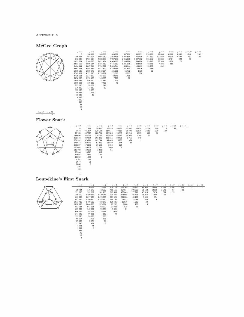
Flower Snarkj = 0

07 878

43 135114 690200 340261 282273 073239 007180 402119 79270 90437 69718 0527 7672 9771 000

28666111

j = 1

7 87861 874

187 515332 265407 935379 816282 743173 80089 92539 50514 7134 5801 150

215251

j = 2

26 617129 158268 795336 780293 485191 74497 65139 50012 7303 220

615805

j = 3

39 815134 515198 500176 070107 13547 40515 5403 760

64065

j = 4

36 19086 88090 38555 57022 7006 2851 145

1255

j = 5

22 83238 39627 21510 9652 715

36920

j = 6

10 62411 9385 3351 240

1401

j = 7

3 7042 531

61060

j = 8

95033030

j = 9

17020

j = 10

19

j = 11

1

Loupekine’s First Snarkj = 0

020 724

121 838350 010663 435941 666

1 073 7201 028 153

852 031623 999409 765243 580131 78665 01429 18711 8454 2911 359

36478121

j = 1

20 724176 872591 662

1 169 8651 617 1331 709 8101 460 5221 044 783

641 221342 967161 26366 82624 3287 7032 073

451716

j = 2

75 758412 502981 968

1 430 0451 470 3051 153 310

723 379373 894162 20259 55418 4814 8101 050

195303

j = 3

124 770490 516862 535930 845703 524398 793176 42562 28217 6223 891

60348

j = 4

126 268367 014475 649373 695201 00678 43222 9165 068

82581

j = 5

89 312190 328177 29997 49135 1668 6881 512

18915

j = 6

46 99871 13345 31516 2533 509

465383

j = 7

18 86419 1167 6381 568

1546

j = 8

5 7663 540

75966

j = 9

1 30940733

j = 10

20922

j = 11

21

j = 12

1

Appendix p. 9

Loupekine’s Second Snarkj = 0

021 156

124 286356 730675 496957 769

1 090 9331 043 540

863 802631 780414 216245 775132 71065 33829 27711 8634 2931 359

36478121

j = 1

21 156180 076601 016

1 185 6281 635 0221 724 5811 469 5551 048 408

641 304341 544159 73265 77223 7767 4752 001

435696

j = 2

76 946417 674991 226

1 439 0861 475 2571 154 068

721 869371 796160 46458 49417 9914 6411 008

189303

j = 3

126 048493 856865 641931 623702 666397 725175 61761 74417 3463 793

58548

j = 4

126 968367 930475 731373 263200 71278 31222 8165 000

80175

j = 5

89 520190 386177 18397 43135 1608 6821 494

18315

j = 6

47 03071 11745 30316 2533 509

465363

j = 7

18 86619 1147 6381 568

1546

j = 8

5 7663 540

75966

j = 9

1 30940733

j = 10

20922

j = 11

21

j = 12

1

Robertson Graphj = 0

01 437 3727 246 700

17 211 69225 936 91328 091 11923 425 65615 702 2948 704 4134 067 4251 622 042

555 756163 80441 3228 8011 540

210201

j = 1

1 437 37212 029 42835 805 21859 406 32065 327 03552 063 83531 670 27415 160 9665 805 5231 786 531

438 57483 92011 9101 128

54

j = 2

6 220 10032 563 39269 906 01186 949 00472 306 44843 319 06619 471 3836 691 3821 760 310

348 28549 4974 552

204

j = 3

12 943 26650 017 89082 616 39080 075 15651 859 11623 931 7008 099 6282 015 912

360 11343 2472 982

72

j = 4

17 896 01854 312 23771 636 75755 598 47328 598 91310 261 3012 594 341

449 94049 4202 802

36

j = 5

18 984 00146 813 70350 385 89731 674 48312 922 3753 532 549

634 47668 9923 652

36

j = 6

16 719 14434 091 28230 117 37615 229 1994 813 247

955 120110 940

6 15072

j = 7

12 772 52621 611 15415 535 1996 178 6191 450 990

193 38612 294

204

j = 8

8 656 42012 056 3886 911 3732 087 824

342 60826 967

642

j = 9

5 255 6405 923 3842 628 658

574 67459 9832 161

j = 10

2 865 5462 549 764

841 681124 393

7 01154

j = 11

1 400 474952 258221 55919 969

418

j = 12

610 470303 94346 2082 128

j = 13

235 46781 0737 182

114

j = 14

79 45817 461

741

j = 15

23 0852 869

38

j = 16

5 643323

j = 17

1 12119

j = 18

171

j = 19

18

j = 20

1

Appendix p. 10

Book(“huck”, 23, 0, 0, 0, 1, 1, 0)j = 0

07 644 119 040

58 063 454 208208 089 907 200468 472 356 864743 860 850 688886 362 588 672823 088 010 752610 456 680 992367 568 054 960181 618 268 88074 123 982 82425 065 464 8107 022 616 8471 625 058 718

308 561 22147 562 7735 855 899

562 02140 5032 061

661

j = 1

7 644 119 040130 942 365 696714 446 189 568

2 122 537 340 1604 123 092 911 0405 729 638 717 4405 999 274 355 7764 889 305 364 2403 167 538 981 0201 653 497 026 704

701 112 177 494242 350 495 65068 266 261 38515 600 933 3832 866 517 167

417 203 23546 993 4653 949 677

233 0958 615

150

j = 2

80 523 030 528911 365 748 352

4 072 619 596 89610 443 363 681 45617 837 338 328 97621 934 086 338 85620 332 420 289 54614 624 737 351 9378 313 631 620 1633 776 758 163 4421 378 712 232 797

404 732 343 62195 166 437 50117 760 717 5392 590 259 291

288 051 46223 498 3321 318 791

45 170704

j = 3

427 469 042 3043 881 430 693 504

14 940 911 766 81633 814 295 549 32851 446 928 857 01656 496 623 747 50446 713 317 299 56629 857 553 469 30114 994 835 055 2665 971 670 244 7331 892 644 074 081

476 705 833 34294 815 567 75714 716 870 8621 749 939 461

155 118 4379 852 285

422 82911 144

144

j = 4

1 534 015 292 83211 932 392 081 45640 626 720 391 89682 361 720 634 568

112 779 195 195 632111 536 656 897 63182 898 207 721 80247 452 347 271 54221 231 473 215 8337 483 614 951 8212 082 708 405 703

456 394 199 83678 141 581 92110 314 463 5821 028 275 760

75 041 7703 809 990

122 0021 895

j = 5

4 208 425 319 23228 958 733 158 88088 689 338 750 268

162 872 521 275 352202 515 265 428 917181 822 039 012 474122 436 175 778 57163 289 339 398 04125 460 955 613 4788 026 773 100 7891 985 823 978 447

384 178 991 07757 622 694 8596 604 985 046

565 949 89335 042 1801 483 706

38 785485

j = 6

9 456 659 968 48858 691 487 844 000

163 670 254 561 170274 803 257 750 421312 764 825 917 711256 878 631 331 512157 948 712 034 29674 347 451 684 55327 140 739 158 9807 732 248 143 9901 720 587 723 236

297 808 086 96639 723 622 6064 020 794 424

301 529 42816 128 290

575 23111 796

86

j = 7

18 198 074 885 356103 243 788 227 460264 694 234 344 442409 580 434 157 718429 835 626 654 435325 285 245 146 851183 994 333 180 12779 489 180 483 32626 556 188 103 0226 900 191 730 7401 394 731 774 739

218 231 222 09326 157 204 3322 360 083 348

155 871 3407 184 647

210 1073 005

j = 8

30 940 731 400 736162 102 328 114 667385 158 972 944 741553 143 680 550 286538 846 162 737 722378 230 381 624 169198 149 002 209 14679 122 703 627 69024 368 441 736 6745 818 100 553 7161 076 252 268 769

153 327 979 45316 622 431 0411 344 595 660

78 646 8163 151 857

77 523862

j = 9

47 560 610 835 303231 997 488 723 635514 385 945 146 530689 925 324 841 686627 608 139 462 721411 029 358 220 644200 617 849 105 61974 482 208 530 19621 270 851 688 2074 692 871 669 682

798 621 154 805104 075 037 50310 246 508 473

745 813 85338 768 9011 352 207

27 469206

j = 10

67 267 401 905 395307 596 180 791 466640 213 989 471 637806 372 976 235 758688 582 006 779 197422 898 675 284 303193 255 210 084 38767 024 385 760 95617 826 935 293 4673 648 698 696 018

573 141 852 73768 506 947 8786 137 792 945

402 557 91318 595 383

561 0139 090

33

j = 11

88 747 842 449 432382 634 254 447 952751 445 805 849 377893 029 971 410 258719 045 082 827 230415 871 654 487 327178 629 421 459 75058 078 504 339 28714 431 482 593 4622 747 096 198 020

399 057 840 81643 803 197 1823 573 570 819

211 208 9198 660 607

224 4832 783

j = 12

110 413 663 746 802451 056 497 992 889839 500 833 190 661945 126 777 109 455720 198 797 592 595393 582 445 653 266159 375 433 931 02948 701 630 168 78911 328 241 057 7602 008 371 282 725

270 019 505 09027 225 629 6302 022 552 038

107 776 8453 932 249

88 116859

j = 13

130 666 491 664 749507 874 432 372 429899 138 156 074 953962 134 122 445 120695 912 053 117 113360 278 181 979 195137 832 995 815 03139 652 159 130 5888 643 948 300 1111 428 133 964 932

177 714 498 46916 453 312 5171 112 678 888

53 497 4841 739 850

33 483234

j = 14

148 114 503 232 862549 640 583 945 429928 434 404 732 381946 802 956 316 230651 526 551 686 197320 142 255 061 978115 885 591 893 63031 417 553 021 9906 421 813 488 934

988 695 612 555113 804 068 059

9 665 564 617594 641 21125 811 941

748 81812 227

53

j = 15

161 710 933 451 019574 575 879 264 822928 302 660 980 981904 076 789 608 510592 898 453 733 529276 885 385 561 80794 920 219 709 71324 262 330 193 5024 649 813 570 718

666 682 299 14070 899 825 3765 515 962 845

308 435 70612 095 111

312 7584 231

8

j = 16

170 813 927 289 507582 448 562 263 319901 802 324 461 765840 089 439 442 061525 705 387 527 193233 534 388 363 80275 855 471 078 62218 280 905 313 3993 283 163 455 432

437 890 395 31242 952 342 2703 055 400 762

155 158 7985 504 691

126 7581 375

j = 17

175 183 508 018 224574 307 823 880 181853 408 768 453 265761 337 884 261 647454 990 478 155 838192 359 454 489 34559 206 435 569 97513 447 888 149 4632 261 157 582 200

280 092 719 25025 286 305 1411 641 278 936

75 679 0902 437 347

50 082428

j = 18

174 936 105 230 968552 153 562 397 919788 339 037 061 129674 053 687 878 178384 901 878 667 513154 895 824 102 50345 166 410 690 8669 661 849 230 1371 518 926 901 479

174 390 514 34214 453 004 774

854 165 57235 781 6671 050 538

19 202121

j = 19

170 475 040 838 235518 597 408 034 174711 981 542 551 881583 766 784 630 227318 587 168 246 233122 026 125 706 54533 691 771 782 4466 780 631 931 834

994 941 569 885105 615 119 324

8 011 736 241430 162 98916 390 015

440 4287 108

31

j = 20

162 410 989 874 779476 549 124 971 777629 449 797 206 205495 042 677 879 502258 204 924 355 94294 096 567 995 26024 580 817 533 0694 647 801 211 901

635 198 727 55862 160 275 5094 301 315 057

209 314 5437 263 816

178 9422 503

7

j = 21

151 482 203 761 928428 948 242 539 842545 264 254 521 678411 367 624 748 301205 018 507 541 18571 045 733 735 89117 540 994 280 5763 110 824 903 986

394 989 616 51035 513 089 0862 232 878 866

98 214 6013 106 323

69 836808

1

j = 22

138 481 043 916 189378 551 418 825 180463 156 138 345 255335 152 391 009 976159 540 234 730 43152 529 965 418 03612 241 838 274 7162 032 190 992 977

239 034 177 69519 668 089 9371 118 570 285

44 326 4081 276 909

25 927231

j = 23

124 191 059 706 563327 779 450 801 827385 979 736 157 458267 823 161 239 724121 698 403 452 62338 034 479 409 3178 353 299 039 1471 294 966 296 360

140 635 158 74310 542 647 994

539 500 32219 181 752

502 0539 067

56

j = 24

109 337 116 734 795278 622 686 027 317315 714 271 443 996209 968 589 993 35491 005 190 493 60726 964 153 070 6205 570 757 950 696

804 342 907 42980 349 078 1225 459 753 151

249 848 0637 926 985

187 5222 949

10

j = 25

94 549 658 362 427232 599 415 134 395253 533 343 091 830161 514 900 952 72066 709 745 029 27518 711 968 201 8153 629 009 765 916

486 565 736 12844 519 508 3302 726 196 170

110 746 6723 111 957

65 933883

1

j = 26

80 342 944 707 533190 758 701 968 316199 919 236 976 320121 905 869 974 53247 926 985 451 59012 706 067 491 3722 307 827 423 945

286 375 736 91323 887 371 3201 309 543 395

46 804 7251 152 202

21 528239

j = 27

67 106 067 181 304153 717 226 791 019154 800 992 492 73590 270 537 601 98133 737 964 980 4548 438 244 908 2751 431 651 832 106

163 814 154 06912 391 822 214

603 613 12418 772 999

398 4236 401

56

j = 28

55 104 744 824 358121 719 136 468 979117 698 380 405 85565 567 617 176 75523 261 782 819 2275 477 591 996 969

865 610 892 67990 962 163 9386 204 115 029

266 217 0547 105 935

127 0181 684

10

j = 29

44 491 423 252 88394 708 476 115 96887 858 171 960 16046 701 038 037 32915 701 786 388 3503 473 196 092 061

509 618 740 84448 964 445 8692 991 921 656

111 984 3862 521 253

36 746380

1

j = 30

35 321 028 354 26772 405 228 468 10064 373 528 302 49532 605 441 633 78110 370 366 228 5632 149 485 588 138

291 838 357 24825 513 055 4411 386 738 494

44 763 707831 602

9 46672

j = 31

27 569 839 915 83954 377 952 292 00046 281 448 067 00422 303 581 464 3186 697 239 653 9801 297 255 575 747

162 366 310 29012 846 282 872

616 213 38116 929 544

252 2022 112

11

j = 32

21 155 277 285 69140 108 145 965 42032 636 626 427 96914 939 530 821 6724 226 027 636 156

762 739 720 15887 644 734 3476 238 791 356

261 761 7866 025 245

69 220386

1

j = 33

15 954 847 768 08829 043 492 273 52422 562 646 009 7209 792 558 415 2542 603 398 119 525

436 426 275 28145 833 115 8842 915 994 723

105 936 8342 004 377

16 80552

j = 34

11 823 018 778 12120 638 880 703 61515 283 132 698 0056 276 719 028 3451 564 280 125 341

242 715 583 85623 180 300 4061 308 416 720

40 682 440617 953

3 4914

j = 35

8 605 270 288 42814 385 457 021 77110 136 458 047 6483 930 854 880 338

915 803 054 713131 021 687 16611 316 367 286

561 964 51814 753 318

174 625589

j = 36

6 149 017 377 5109 828 892 336 5386 577 897 351 1812 403 021 466 599

521 796 689 08568 546 193 8425 320 896 693

230 239 0725 022 558

44 54873

j = 37

4 311 436 549 8116 578 623 394 3994 173 019 367 6541 432 512 031 399

288 971 661 58834 695 422 1222 403 511 898

89 612 5691 593 264

10 0315

Appendix p. 11

j = 38

2 964 474 698 9574 310 052 558 6972 585 645 699 396

831 790 371 315155 326 381 06716 957 718 1111 039 924 955

32 969 506466 505

1 925

j = 39

1 997 470 496 0582 761 684 207 3951 563 111 427 998

469 846 262 71280 906 285 7327 985 680 153

429 469 51611 395 789

124 530297

j = 40

1 317 887 697 6731 728 990 256 047

920 894 742 411257 819 091 78140 765 822 5753 614 180 128

168 586 7893 672 196

29 81533

j = 41

850 665 829 4041 056 510 698 738

528 044 208 920137 219 085 70619 829 960 2501 567 456 613

62 586 2691 092 398

6 2612

j = 42

536 654 329 284629 363 523 349294 272 153 26770 712 799 8909 291 403 735

649 222 79221 837 068

296 1341 117

j = 43

330 528 626 041365 006 585 603159 130 489 57435 214 172 5064 182 750 513

255 780 2137 105 191

71 881161

j = 44

198 505 264 692205 792 941 63783 350 267 19016 908 923 2641 803 797 937

95 399 6652 134 376

15 23817

j = 45

116 089 433 466112 609 389 06642 202 405 3607 809 196 055

742 649 89333 492 231

584 1822 717

1

j = 46

66 010 296 07059 693 833 14720 608 991 4523 458 946 792

290 757 07310 990 747

143 089383

j = 47

36 432 673 76230 590 692 1199 681 466 5321 464 504 260

107 745 7983 342 402

30 57538

j = 48

19 480 581 01215 119 155 3544 362 140 777

590 430 01537 582 223

931 8955 485

2

j = 49

10 069 527 3617 187 420 8931 878 612 930

225 629 51312 256 579

234 974776

j = 50

5 019 400 8193 276 272 681

770 201 91281 283 4543 706 816

52 64177

j = 51

2 406 133 6961 426 882 777

299 178 40127 422 3571 029 033

10 2324

j = 52

1 105 659 524591 250 737109 478 461

8 592 757258 783

1 668

j = 53

485 226 772231 936 33037 477 4932 474 897

57 926216

j = 54

202 490 44185 622 59911 898 600

646 35511 258

20

j = 55

79 941 54929 531 0123 465 267

150 2771 830

1

j = 56

29 674 4849 430 560

912 61730 308

234

j = 57

10 280 2102 757 016

213 2155 101

21

j = 58

3 293 359727 12343 020

6731

j = 59

964 438169 643

7 20562

j = 60

254 35334 073

9403

j = 61

59 2285 661

85

j = 62

11 848730

4

j = 63

1 95665

j = 64

2503

j = 65

22

j = 66

1