EXPONENTIAL STABILITY FOR TIME DEPENDENT POTENTIALS

A. GIORGILLIDipartimento di Matematica dell’Universita,

Via Saldini 50, 20133 MILANO, Italy

E. ZEHNDERForschunginstitut fur Mathematik ETH, CH–8093 ZURICH, Switzerland

Abstract. For a classical Hamiltonian system on a torus defined by a time dependent,

bounded and analytic potential we establish global and quantitative bounds for the solutions

over an exponentially long interval of time by using techniques which go back to Nekhoroshev.

Contents:1. Introduction and results.2. Local normal forms.3. Geography of resonances.4. Global estimates depending on parameters.5. Choice of the parameters, Proof of theorem 2.6. Existence of the normal form.

18.10.1991

2

1. Introduction and results

On the phase space Tn×Rn we consider a time–dependent Hamiltonian system givenby the Hamiltonian function

(1) H(x, y, t) =1

2|y|2 + V (x, t) ,

where (x, y) ∈ R2n and t ∈ R, and where V depends periodically on x:

(2) V (x+ j, t) = V (x, t) , j ∈ Zn .

It is, of course, well known that, in general, the flow of the corresponding Hamiltoniansystem

(3)x =

∂

∂yH(x, y, t)

y = − ∂

∂xH(x, y, t)

is extremely complicated. If the potential V , however, is bounded, the system can beviewed as a system close to an integrable one in the region of the phase space where|y| is large; the integrable system is given by H(y) = 1

2 |y|2. Therefore, one might betempted to ask whether for the flow ϕt

(

x(0), y(0))

=(

x(t), y(t))

of (3) one has

(4) supt∈R

|y(t)| <∞ ,

i.e., whether all the solutions are bounded for all times.In the special case, n = 1, this can indeed be proven for potentials which depend,

in addition, periodically on time t and which are sufficiently smooth[1][2][3]. More gen-erally, if the potential is quasiperiodic in time, with frequencies (ω1, . . . , ωN ) satisfyingdiophantine conditions, it can be shown that all the solutions are bounded on the wholetime interval, provided V as a function on T1×TN is sufficiently smooth. The boundsfor the solutions are deduced from the existence of quasiperiodic solutions[4][1].

The situation is quite different in the case n > 1. If the potential is quasiperiodicin time, V = V (x, ωt), then there still exists an abundance of quasiperiodic solutions,hence of solutions which are bounded for all times, provided V is sufficiently smooth[1].However, in sharp contrast to the case n = 1, the quasiperiodic solutions do not givebounds for all solutions, since the invariant surfaces covered by the quasiperiodicsolutions do not bound open sets in the phase space, and boundedness of all solutionscannot be expected.

Recall now that for systems of the form H(x, y) = H0(y)+ εH1(x, y) on Tn×Rn

and ε small N. N. Nekhoroshev[5] discovered estimates for all solutions, not over thewhole time interval, but over an exponentially long interval of time, assuming theHamiltonian to be not only smooth, but real analytic, and assuming, moreover, theintegrable systemH0 to meet certain convexity type conditions. In view of these resultsone might guess that such exponential estimates hold true also for our global problem.This is indeed the case, as we shall prove.

3

In order to formulate the result we assume V (x, t) to be real analytic and, more-over, to have a holomorphic extension to a complex strip | Imx| < 2σ and | Im t| < 2σfor some σ > 0, such that

(5) |V |2σ = sup| Im x|<2σ| Im t|<2σ

|V (x, t)| <∞ .

Denote by B(R) the open ball in Rn centered at 0 with radius R > 0. Then thefollowing statement of exponential stability replaces (4) in higher dimensions.

Theorem 1: Let ϕt(

x(0), y(0))

=(

x(t), y(t))

be the flow of the Hamiltonian vectorfield (3) on Tn × Rn. Assume the potential V (x, t) is real analytic on Tn × R andhas an analytic extension to a complex strip 2σ > 0 satisfying (5). Then there are twopositive constants R∗ and T∗ depending on |V |2σ, σ and the dimension n, such thatfor R ≥ R∗ the following statement holds true: if y(0) ∈ B(R) then y(t) ∈ B(2R) forall t in

|t| ≤ T∗ exp

(

R

R∗

)1/a

, with a =n2 + n

2.

The constants are given by

T∗ =σ

8e2

R∗ = Ka∗

2n+3(n+ 1)!

e

(

1 + e−σ/2

1− e−σ/2

)n

|V |2σ

where K∗ is the smallest positive integer satisfying

K∗ ≥ 25e4n

σ

(

1− e−σ/2

1 + e−σ/2

)n1

|V |2σand K∗ ≥ 5

σ.

Observe that there is no smallness requirement on the potential V ; however, Vis assumed to be real analytic and to have a bounded holomorphic extension in acomplex strip. The statement applies in particular to a potential V which dependsquasiperiodically on time t, V = V (x, ωt) with V (x, ξ) being real analytic and periodicin all the variables (x, ξ) ∈ Tn ×TN ; the frequency vector ω ∈ RN is not required tomeet diophantine conditions.

The above theorem follows immediately from the following stronger statement.

Theorem 2: Let ϕt(

x(0), y(0))

=(

x(t), y(t))

be the flow of the Hamiltonian vec-tor field (3) on Tn × Rn. Assume the potential V (x, t) satisfies the assumptions oftheorem 1. Then

dist(

y(t), y(0))

<

for all t in

|t| ≤ T∗ exp

(

∗

)1/a

with a =n2 + n

2,

4

and for all ≥ ∗. The constants ∗ = R∗ and T∗ are defined in theorem 1.

As a sideremark we should mention that the exponent a is equal to 1 in the specialcase n = 1. Hence one concludes for all solutions of forced pendulum like equationsdefined by Hamiltonians of the form

H(x, y, t) =1

2y2 + V (x, t)

with V periodic in x, the estimate

|y(t)− y(0)| <

for all t in

|t| ≤ T∗ exp

(

∗

)

and for all ≥ ∗.It should be recalled that the so called steepness of the “integrable part”, which

in our case is H0(y) = |y|2/2, is crucial for estimates over a time interval whichis exponentially large. This is illustrated by the following example of an even timeindependent system due to N.N. Nekhoroshev[5]:

H(x, y) =1

2(y21 − y22) + sin(x1 − x2) .

The special solution

(

y∗1(t), y∗2(t), x

∗1(t), x

∗2(t)

)

=(

−t, t,−1

2t2,−1

2t2)

satisfiesdist

(

y∗(t), y∗(0))

=√2 |t|

for all t ∈ R, in sharp contrast to the statement in theorem 2.We observe that rescaling the action and the time by setting

y =1

εη and t = ετ

leads to the Hamiltonian system described by the function

H(x, η, τ) =1

2|η|2 + ε2V (x, ετ) ,

which is equivalent to (1) and instead of studying solutions of (1) for large y wetherefore can as well study solutions for bounded |y| choosing ε small. This is anadiabatically perturbed system to which the ideas of Nekhoroshev [5] apply.

Indeed, the proof of theorem 2 is based on the underlying ideas of Nekhoroshev[5]

and of Benettin, Galgani and Giorgilli[6]. Actually, it turns out that the proof requiresonly minor modifications of the latter work. However, some extra work is neededbecause the time dependence is not assumed to be periodic or quasiperiodic. Forthis reason also the approach by Benettin and Gallavotti[7], the simplified version ofNekhoroshev’s theory due to P. Lochak[8] and the recent elegant and quantitatively

5

improved approach to Nekhoroshev’s estimates due to J. Poschel do not apply directlyto our problem.

2. Local normal forms

It is a convenient trick to remove the time dependence by simply extending the phasespaceRn×Tn by two additional variables (ξ, η) ∈ R2, which are canonically conjugate,and to consider the Hamiltonian function

(6) H(x, y, ξ, η) =1

2|y|2 + η + V (x, ξ) .

The following part of the Hamiltonian equations

(7)

x =∂

∂yH(x, y, ξ, η) = y

y = − ∂

∂xH(x, y, ξ, η) = −Vx(x, ξ)

ξ =∂

∂ηH(x, y, ξ, η) = 1

is then independent of η and obviously equivalent to (3).As usual, instead of solving the equations we shall make use of the Hamilto-

nian transformation theory in order to find local normal forms for the Hamiltonianfunctions. Since the ξ variable is distinguished, the symplectic diffeomorphisms ϕ con-sidered later on in the transformation theory will belong to the following subgroup Sof symplectic diffeomorphisms:

S = {ϕ = id + ψ | ψ = ψ(x, y, ξ) and ξ remains fixed} .Examples of such diffeomorphisms are the maps belonging to the flow of a Hamiltonianvector field whose Hamiltonian function does not depend on the variable η.

In order to describe those subsets of the phase space on which the Hamiltonianwill be transformed into normal form we need some definitions.

Definition 1: Resonance module. If M ⊂ Zn is a subgroup we denote by PM ⊂ Rn

the real subspace generated by M , and call the subgroup of Zn, defined by

(8) M = PM ∩ Zn ,

a resonance module. The integer dimPM will be called the dimension or multiplicityof the resonance module.

To a real domain G ⊂ Rn and δ > 0 we shall associate the complex neighbourhood

(9) Gδ = {y ∈ Cn | |y − G| < δ}and denote by G(δ,σ) the complex domain

(10) G(δ,σ) = Gδ × {η ∈ C} × {| Imx| < σ} × {| Im ξ| < σ} .

6

Definition 2: Nonresonance domain. A set G ⊂ Rn is called a nonresonance domainof type (M, α, δ,N) if

|k · y| > α for all y ∈ Gδ , k ∈ Zn \M and |k| ≤ N .

Here, |k| = |k1|+ . . .+ |kn|, α and δ are real positive parameters, N a positive integerand M a resonance module.

After these preliminaries we are ready to formulate the analytical ingredient ofthe proof of the theorem.

Proposition 1: Normal forms on nonresonance domains. Let r and K be positiveintegers, and let N = rK. Moreover, let G ⊂ Rn be a nonresonance domain of type(M, α, δ,N). Then, there are positive constants A and B depending on |V |σ, σ, δ andn such that if

(11) ε :=

(

rA

α+ 2e−Kσ/2

)

≤ 1

2

there exists a real analytic symplectic diffeomorphism ϕ belonging to the subgroup S,such that ϕ and ϕ−1 are defined on the complex domain G(δ,σ) 1

2and satisfy

(12) dist(y, ϕ(y)) ≤ 1

4δ , dist(y, ϕ−1(y)) ≤ 1

4δ .

The map ϕ transforms the Hamiltonian H into the following normal form on G(δ,σ) 12:

(13) H ◦ ϕ =1

2|y|2 + η +NM +R ,

where

(14) NM =∑

k∈M|k|≤N

fk(y, ξ)eik·x .

The remainder R satisfies, on G(δ,σ) 12, the estimate

(15) |R| ≤ Bεr .

Moreover:

(16) G(δ,σ) 14⊂ ϕ

(

G(δ,σ) 12

)

⊂ G(δ,σ) 34.

In addition, the same statement holds true for ϕ−1 instead of ϕ. The constants aregiven by

A =25en

δσ

[

(

1 + e−σ/2

1− e−σ/2

)n

|V |2σ +eδ

2

]

B = 2

(

1 + e−σ/2

1− e−σ/2

)n

|V |2σ .

The proof of the statement, based on a recursion procedure, is postponed to sect. 6below. The ultimate aim is, of course, to choose the parameters such that εr is small.

7

The proposition allows us to gain already some crucial insight into the flow of (7)at least locally on G. Namely, we conclude immediately that the functions Iµ defined,in the new variables on G(δ,σ) 1

2, by

(17) Iµ = µ · y , µ ∈ Rn and µ ⊥ M ,

are approximate integrals. Indeed, computing the time derivative along a solution ofH ◦ ϕ we obtain

d

dtIµ = µ · d

dty = µ · ∂

∂x(H ◦ ϕ) = i

∑

k∈M

(µ · k)fk(y, ξ)eik·x + µ · ∂∂x

R .

Since µ · k = 0 for k ∈ M, we find the estimate, on Gδ/2 ×Tn × {| Im ξ| < σ/2},

(18)

∣

∣

∣

∣

d

dtIµ

∣

∣

∣

∣

≤ 2|µ|σBεr ,

where we have used (15) and the Cauchy estimate in order to estimate the derivative ofa holomorphic function in terms of the supremum of the function. This consequence ofthe proposition 1 leads to the proposition 2 below in the original nonresonance domainG ⊂ Rn. In order to formulate it we need a definition.

If M is a resonance module and y∗ ∈ Rn we define the plane PM(y∗) containingy∗ by

(19) PM(y∗) = {y ∈ Rn | y = y∗ + PM} ,

where PM is introduced in definition 1.

Proposition 2: Assume the potential V (x, t) is real analytic and bounded on thecomplex strip | Imx| < 2σ and | Im t| < 2σ for some σ > 0. Let r and K be positiveintegers, N = rK. Assume G ⊂ Rn is a nonresonance domain of type (M, α, δ,N).Then there are positive constants A and C depending on |V |2σ, σ, δ and n such thatif

ε :=

(

rA

α+ 2e−Kσ/2

)

≤ 1

2

then, the following holds true: if(

x(t), y(t), ξ(t), η(t))

is a solution of the Hamiltoniansystem (6) satisfying y(0) ∈ G and y(t) ∈ G for τ− < t < τ+, then

dist(

y(t), PM(y(0)))

≤ 3

4δ

for t ∈ [τ−, τ+] ∩ [−t∗, t∗] , wheret∗ = Cε−r .

The constant A is defined in proposition 1, and C is defined by

C =δσ

8B,

with B as in proposition 1.

8

Figure 1. Confinement of the orbit in the strip around the plane PM(y(0)),unless it leaves the domain G.

Proof. Let ϕ be the symplectic diffeomorphism of proposition 1, and, in abuse ofnotation, let y = ϕ(y′); then

|µ ·(

y(t)− y(0))

| ≤ |µ ·(

y(t)− y′(t))

|+ |µ ·(

y′(t)− y′(0))

|+ |µ ·(

y′(0)− y(0))

| .

Taking the supremum over µ ∈ Rn with |µ| = 1 and µ ⊥ M, the first and the thirdterm on the right hand side are estimated by δ/4 in view of the properties (12) of thediffeomorphism ϕ, while the second term is estimated, in view of (18), by

|y′(t)− y′(0)| ≤ |t| · 2σ|R| ,

which is smaller than δ/4, if |t| ≤ t∗, in view of the estimate for |R| in proposition 1.This finishes the proof of proposition 2. Q.E.D.

If a solution leaves the local domain G considered above in a time shorter than t∗

we, of course, loose control (see fig. 1) and are forced to study the geometric patternof all possible nonresonance domains. This will be done in the next section, where thespecial form of the integrable part which is given by H0 = |y|2/2 allows a simplificationof earlier presentations.

3. Geography of resonances

If G ⊂ Rn is an open set and > 0 we denote by G − the subset

G − = {y ∈ G | B(y, ) ⊂ G} ,

9

where B(y, ) is the open ball of radius and center y. We shall first recall someconcepts from [5] and [6]. We point out that we shall need only G = Rn for ourpurpose.

1. N–moduli and resonance parameters. If M ⊂ Zn is a resonance module and Na positive integer we introduce the abbreviation

(20) MN = {k ∈ M | |k| ≤ N}

and call a module M of dimM = s an N–module if MN contains s independentvectors k ∈ Zn. To the N–moduli of dimM = s we associate a positive parameter βssuch that β0 < β1 < . . . < βn. They will be determined below.

2. Resonant manifold. With an N–module M we associate the resonant manifoldΣM defined by

(21) ΣM = {y ∈ Rn | k · y = 0 for all k ∈ M} .

3. Resonant zone. With an N–module M of dimM = s we associate the resonantzone ZM defined by

(22)ZM = {y ∈ G − | there are s independent

k ∈ MN such that |k · y| < βs}

4. Resonant region of order s. To the family of all N–moduli M of fixed dimM = swe associate the subset

(23) Z∗s =

⋃

dimM=s

ZM .

By definition, Z∗0 = G − ; we also set Z∗

n+1 = ∅.5. Resonant block. For an N–module M of dimM = s we define the associatedresonant block BM ⊂ Rn to be the subset of G − :

(24) BM = ZM \ Z∗s+1 .

6. Resonant plane. To y ∈ BM we associate the resonant plane

(25) PM(y) = {y + w | w ∈ PM} .

7. Extended plane. For δ > 0 and y ∈ BM, the extended plane is defined to be theset

(26) PM,δ(y) ={

z ∈ Rn | dist(

z, PM(y))

≤ δ}

.

8. Cylinder and its basis. For y ∈ BM and δ > 0 the cylinder is defined to be the set

(27) CM,δ(y) = PM,δ(y) ∩ ZM ;

its basis is defined as ∂ZM ∩ PM,δ(y).

10

Figure 2. The geography of the resonances in the plane case. Multiplicity 2:

the resonant manifold is the point O; the resonant zone, region and block are

the square–shaped area ABCD. Multiplicity 1: the resonant manifolds are the

curves ΣM and ΣM′ , which intersect in the point O; the resonant zones are the

strips around these curves; the resonant region is the cross-shaped area formed

by the union of the strips, the resonant blocks are the dashed parts of the strips.

Multiplicity 0: the resonant manifold, zone and region are the whole domain;

the resonant blocks are the complement of the cross-shaped area which is the

resonant region of multiplicity 1.

9. Extended resonant block. The extended resonant block is defined to be the set

(28) BM,δ =⋃

y∈BM

CM,δ(y) .

The crucial sets in the following are the resonant blocks BM. In view of the nextlemma they are the likely candidates of the distinguished sets in Rn which meet theassumptions in proposition 1.

11

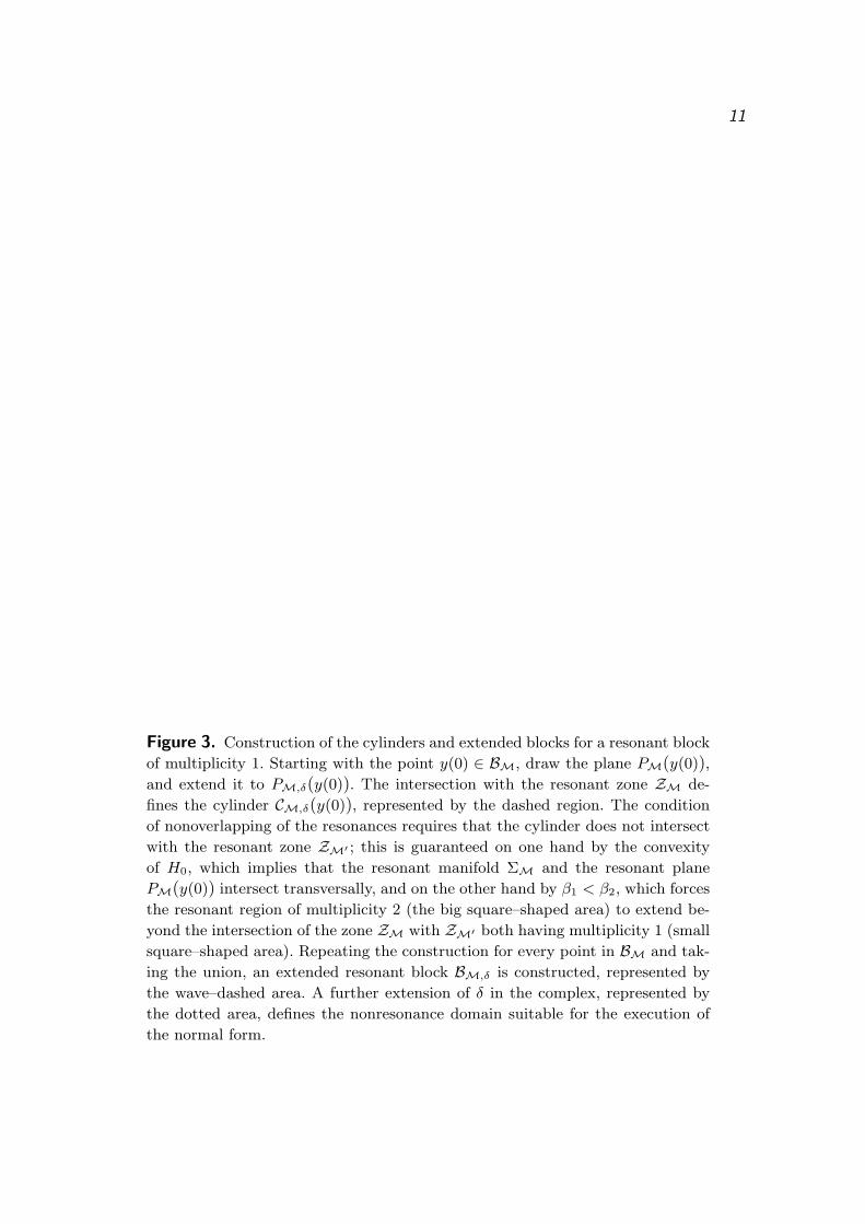
Figure 3. Construction of the cylinders and extended blocks for a resonant block

of multiplicity 1. Starting with the point y(0) ∈ BM, draw the plane PM(y(0)),and extend it to PM,δ(y(0)). The intersection with the resonant zone ZM de-

fines the cylinder CM,δ(y(0)), represented by the dashed region. The condition

of nonoverlapping of the resonances requires that the cylinder does not intersect

with the resonant zone ZM′ ; this is guaranteed on one hand by the convexity

of H0, which implies that the resonant manifold ΣM and the resonant plane

PM(y(0)) intersect transversally, and on the other hand by β1 < β2, which forces

the resonant region of multiplicity 2 (the big square–shaped area) to extend be-

yond the intersection of the zone ZM with ZM′ both having multiplicity 1 (small

square–shaped area). Repeating the construction for every point in BM and tak-

ing the union, an extended resonant block BM,δ is constructed, represented by

the wave–dashed area. A further extension of δ in the complex, represented by

the dotted area, defines the nonresonance domain suitable for the execution of

the normal form.

12

Lemma 1: Let M be an N–module of dimM = s. Then for every y ∈ BM thefollowing nonresonance condition holds true:

|k · y| ≥ βs+1 if k 6∈ M and |k| ≤ N .

Proof. Assume, by contradiction, that there is a y ∈ BM and a k 6∈ M with |k| ≤ Nsatisfying |k · y| < βs+1. Since BM ⊂ ZM, and since, by assumption, βs < βs+1 weconclude from the definition of ZM that there are s + 1 independent vectors k ∈MN satisfying |k · y| < βs+1. Consequently, y ∈ ZM′ for a resonant N–module M′

with dimM′ = s + 1. Therefore, y ∈ ZM′ ⊂ Z∗s+1, and so y 6∈ BM = ZM \ Z∗

s+1,contradicting y ∈ BM. Q.E.D.

We next define the parameters in terms of N , and n.

Definition 3: Let N be a positive integer and let > 0. Then we set

β0 =[

2n+1(n+ 1)!N (n2+n−2)/2]−1

,

βs = 2ss!N [s(s−1)]/2β0 for 1 ≤ s ≤ n ,

and

δs =βs2N

for 0 ≤ s ≤ n .

It then follows that

(29)β0 < β1 . . . < βn

δ0 < δ1 . . . < δn < .

The main result of this section is the following

Proposition 3: Let N be a positive integer, let > 0 and consider the domainG − ⊂ Rn. Then1) Covering:

G − ⊂⋃

M

BM .

2) For 0 ≤ s ≤ n

(G − ) \ Z∗s+1 ⊂

⋃

0≤dimM≤s

BM .

3) If M is a N–module of dimM = s, then for every y ∈ BM

diam CM,δs(y) < .

4) If M and M′ are N–moduli of dimM = dimM′ = s, then

ClosBM,δs ∩ ZM′ = ∅ if M 6= M′ .

5) For an N–module M of dimM = s

(BM,δs)δs ∩Rn ⊂ G .

13

6) If M is a N–module of dimM = s, then for every y belonging to the complexdomain (BM,δs)δs the following nonresonance condition holds true

|k · y| ≥ βs2

if k 6∈ M and |k| ≤ N .

Proof of proposition 3. The statements 1 and 2 follow readily from the definition.Indeed, observe that

⋃

dimM=s

BM =⋃

dimM=s

(

ZM \ Z∗s+1

)

=⋃

dimM=s

ZM \ Z∗s+1 = Z∗

s \ Z∗s+1 .

For s = 0, we have Z∗0 = G − , which proves statement 2 for s = 0. For s > 0 we

proceed by induction assuming statement 2 to be true up to s− 1; then

(G − ) \ Z∗s+1 = [(G − ) \ Z∗

s ] \ Z∗s+1 ∪

(

Z∗s \ Z∗

s+1

)

⊂(

⋃

dimM<s

BM

)

\ Z∗s+1 ∪

(

⋃

dimM=s

BM

)

⊂⋃

dimM≤s

BM .

Setting s = n the statement 1 follows, since Z∗n+1 = ∅. In order to prove statement 3

we need the following geometric lemma which is of independent interest and which isproved in [6], appendix B:

Lemma 2: Let 1 ≤ s ≤ n, and let (u(1), . . . , u(s)) be linearly independent vec-tors in Rn satisfying |u(j)| ≤ N for some positive N and for 1 ≤ j ≤ s, and de-note by Vol(u(1), . . . , u(s)) the s–dimensional volume of the parallelepiped with sidesu(1), . . . , u(s); let, moreover, w ∈ span(u(1), . . . , u(s)), and α be a positive constant.Then, the following statement holds true: if |w · u(j)| ≤ α for 1 ≤ j ≤ s, then theEuclidean norm of w is bounded by

‖w‖ < sNs−1α

Vol(u(1), . . . , u(s)).

We shall conclude from lemma 2

Lemma 3: Let M be an N–module of dimM = s. Then for y ∈ BM

diam CM,δs(y) < 2sNs−1βs + 2δs .

Proof. Changing the notation we recall that

CM,δs(y0) = ZM ∩ PM,δs(y0) for y0 ∈ BM .

Let now y ∈ CM,δs(y0) and pick y∗ ∈ PM(y0) such that y − y∗ ⊥ PM. In view of thedefinition of PM,δs(y0) we conclude that

(30) dist(y, y∗) ≤ δs .

14

Pick y ∈ PM(y0) ∩ ΣM; then k · y = 0 for k ∈ M, and we conclude, since y − y∗ ⊥PM(y0), that

k · y = k · (y − y)

= k · (y − y∗) + k · (y∗ − y)

= k · (y∗ − y) .

Since y ∈ ZM there are s independent vectors k ∈ MN such that |k · y| < βs.Consequently,

|k · (y∗ − y)| < βs

for these vectors, and since y∗ − y ∈ PM we conclude by lemma 2,

(31) dist(y∗, y) ≤ sNs−1βs .

Using the triangle inequality we find by (30) and (31) that dist(y, y) ≤ sNs−1βs + δs.Therefore, if y1 and y2 ∈ CM,δs(y0) we can estimate, again by the triangle inequality,dist(y1, y2) ≤ 2sNs−1 + 2δs. The proof of the lemma is finished. Q.E.D.

In view of the definition of the sequences βs and δs we conclude in particular fromlemma 3 that diam CM,δs(y) < for y ∈ BM, as claimed in statement 3.

Next, we claim that if y ∈ BM,δs then

(32) |k · y| ≥ βs for k 6∈ M and |k| ≤ N .

Indeed, in view of the definition of BM,δs , there exists a y′ ∈ BM such that y ∈CM,δs(y

′), and, by lemma 1, we have |k·y′| ≥ βs+1. Moreover, by the previous lemma 3,

|k · (y′ − y)| ≤ |k| dist(y′, y) ≤ N diam CM,δs(y′) < N(2sNs−1βs + 2δs) .

Consequently,

|k · y| ≥ |k · y′| − |k · (y′ − y)| ≥ βs+1 −N(2sNs−1βs + 2δs) ,

which is ≥ βs by our choice of the sequences in definition 3. This proves the claim (32).In order to prove statement 6 let y ∈ (BM,δs)δs . By definition of the complex ex-

tension there exists an y′ ∈ BM,δs such that |y′j−yj | ≤ δs for 1 ≤ j ≤ n. Consequently,if |k| ≤ N ,

|k · (y′ − y)| ≤ δs∑

|kj | ≤ Nδs ≤1

2βs ,

by our choice of the sequences. Therefore, in view of (32), if k 6∈ M then

|k · y| ≥ |k · y′| − |k · (y′ − y)| ≥ 1

2βs ,

as claimed in statement 6.In order to prove statement 4 assume, by contradiction, that y ∈ BM,δs∩ZM′ 6= ∅.

Since y ∈ ZM′ and M 6= M′, there is a k 6∈ M, |k| ≤ N , such that |k · y| < βs, incontradiction to estimate (32). Finally, the statement 5 is readily verified using thedefinition of the sequence δs. The proof of proposition 3 is complete. Q.E.D.

15

4. Global estimates depending on parameters

The previously described geography of resonances provides us with domains in Rn

which cover Rn and which meet the assumptions of the local analytic statement inproposition 1. In order to reformulate proposition 2 we shall introduce the

Definition 4: Assume(

x(t), y(t), ξ(t), η(t))

is a solution starting in y(0) ∈ IntG forsome set G ⊂ Rn. The exit resp. entrance time of this solution in G is defined as

τ+ = sup {t > 0 | y(s) ∈ IntG for 0 ≤ s ≤ t}resp.

τ− = inf {t < 0 | y(s) ∈ IntG for t ≤ s ≤ 0} .

The parameters βs and δs occurring in the following lemma are defined in defini-tion 3. It should be recalled that they do depend on the parameters N and .

Lemma 4: Let r and K be positive integers, N = rK and let > 0 and σ > 0.Consider the N–module M of dimM = s with the associate parameters βs and δs.With the constants A and B depending on |V |σ, σ, n and δ = δs as in proposition 1we set

εs =2rA

βs+ 2e−Kσ/2

t∗s =δσ

8Bε−rs .

Assume εs ≤ 1/2. Then for a solution with y(0) ∈ BM and with exit (resp. entrance)time τ+ (resp. τ−) in the cylinder CM,δs

(

y(0))

the following holds true: if τ+ ≤ t∗s(resp. if τ− ≥ −t∗s) then

y(τ+) (resp. y(τ−) ) ∈(

∂ZM ∩ PM,δs

(

y(0)))

.

In other words a solution with y(0) ∈ BM ∩ CM,δs

(

y(0))

can leave the cylinder

CM,δs

(

y(0))

within the time interval |t| ≤ t∗s only through its base (see fig. 3).

Proof. By assumption y(0) ∈ BM ∩ CM,δs

(

y(0))

. By definition BM ⊂ BM,δs . Inview of proposition 3, statement 6, the set BM,δs satisfies the assumptions of Gin proposition 2, with δ, however, replaced by δs and α replaced by βs/2. SinceCM,δs

(

y(0))

⊂ BM,δs we, therefore, conclude from proposition 2 that if τ+ ≤ t∗s, then

y(τ+) ∈ IntPM,δs . Moreover, by definition of the exit time, y(τ+) ∈ ∂CM,δs

(

y(0))

,

so that y(τ+) ∈ ∂CM,δs

(

y(0))

∩ IntPM,δs

(

y(0))

, as claimed. Similarly for τ− andy(τ−) if τ− ≥ t∗s. From the definition of the corresponding sets one concludes readilythat

(

∂CM,δs

(

y(0))

∩ IntPM,δs(y(0)))

⊂(

∂ZM ∩ PM,δs(y(0)))

, and this finishes theproof. Q.E.D.

The crucial step in proving theorem 1 is the following lemma, which combines theanalytical and the geometrical considerations.

Lemma 5: With the parameters r, K, N = rK, > 0 and σ > 0 given, with theconstants A and B depending on |V |σ, σ, n and δ = δ0, and with δ0 and β0 as given

16

in definition 3, define

ε0 =2rA

β0+ 2e−Kσ/2

T ∗0 =

δσ

8Bε−r0

and assume ε0 ≤ 1/2. If a solution satisfies y(t) ∈ G − for t ∈ [a, b], then

dist(y(t), y(s)) <

for all t, s ∈ [a, b], provided b− a < T ∗0 .

Proof. We shall prove the existence of a resonance module of dimM = s for somes such that

(33) y(t) ∈ CM,δs(y∗) for t ∈ [a, b] .

The lemma then follows in view of diam CM,δs

(

y∗)

< , which is the statement 3 ofproposition 3. In order to prove (33) observe that due to the statement 1 in proposi-tion 3 there exists for every t ∈ [a, b] a N–module Mt such that y(t) ∈ Mt, which hasminimal dimension. Since the set of all N–moduli is finite there exists among theseN–moduli Mt, t ∈ [a, b], a N–module M such that dimM = s is minimal. Theny(t0) ≡ y∗ ∈ BM for some t0 ∈ [a, b]. Let now τ+ be the exit time of the solutiony(t) starting at y∗ contained in the cylinder CM,δs(y

∗), and assume that τ+ ≤ t∗0. Weclaim that

(34) y(t0 + τ+) ∈ ∂ZM ∩ PM,δs(y∗) .

Indeed, by definition, β0 < βs and δ0 < δs. Moreover, A(δ0) ≥ A(δs) and B(δ0) =B(δs), so that ε0 > εs and consequently t∗0 < t∗s. The claim (34) follows thereforeimmediately from the previous lemma 4. Next we claim that

(35) b < t0 + τ+ .

Indeed, assume by contradiction that b ≥ t0+τ+. Then we conclude that y(t0+τ

+) ∈G − , and, by (34), that y(t0 + τ+) 6∈ ZM. Since, by proposition 3, statement 4,ClosBM,δs ∩ ZM′ = ∅ for every M′ 6= M satisfying dimM = dimM′ = s we find

y(t0 + τ+) 6∈⋃

dimM=s

ZM = Z∗s .

Therefore, y(t0 + τ+) ∈ (G − ) \ Z∗s . But, by proposition 3, statement 2,

(G − ) \ Z∗s ⊂

⋃

dimM=s−1

ZM .

Consequently, y(t0 + τ∗) ∈ BM∗with dimM∗ ≤ s− 1. Since t0 + τ+ ∈ [a, b] this con-tradicts the definition of M which is assumed to have minimal dimension. Therefore,the claim b < t0 + τ+ is proved. The same arguments show that a > τ−, and weconclude that y(t) ∈ CM,δs(y

∗) for all t ∈ [a, b], as claimed in (33). This proves thelemma. Q.E.D.

17

Assume now y(0) ∈ G − 2, and pick as time interval [a, b] = [τ−, τ+], where τ+

and τ− are the exit and entrance times of an orbit starting from y(0) in the center ofopen ball of radius :

a =sup{t > 0 | dist(y(s), y(0)) < for s ∈ [0, t]}b =sup{t > 0 | dist(y(s), y(0)) < for s ∈ [−t, 0]} .

From lemma 5 one concludes immediately

Proposition 4: Let r, K, N = rK, > 0, σ > 0, A and B be as in lemma 5. Thenfor every solution with y(0) ∈ G − 2

dist(y(t), y(0)) < if |t| ≤ T ∗0 =

δσ

8Bε−r0 ,

provided ε0 ≤ 1/2.

It remains to choose the parameters N ≥ 1 and r ≥ 1 for given and σ > 0, sothat ε0 ≤ 1/2 and such that T ∗

0 is as large as possible.

5. Choice of the parameters, Proof of theorem 2

In view of Proposition 4 it remains to choose the parameters in order to verify theo-rem 2. For given > 0 and σ > 0 the parameters to be chosen are r, K and N , whererK = N . In order to first describe the idea of our choice recall the definition of theparameters β0 and δ0 in definition 3, which depend on , and recall also the definitionof the constants A and B in Proposition 1. We abbreviate for the following

a =n2 + n

2.

Then, for given > 0 we first choose

N =

(

0

)1/a

with an arbitrary dimensional constant 0; this gives

(36) δ0 =β02N

=0

2n+2(n+ 1)!.

Consequently, A and B are also determined. In order to choose K recall that rK = N ,and compute

(37) ε0 =2rA

β0+ 2e−Kσ/2 =

C

K+ 2e−Kσ/2

with C = A 2n+2(n+ 1)! . We finally choose K = K∗ so large that

ε0 ≤ 1

e

18

as required in Proposition 4. We conclude that the time T ∗0 is indeed estimated expo-

nentially by

(38) T ∗0 = T∗ε

−r0 ≥ T∗ exp

(

N

K∗

)

= T∗ exp

(

∗

)1/a

with T∗ = δσ8B and

∗ = Ka∗0 .

Since rK∗ = N = (/0)1/a and K∗ and r are positive integers we get the condition

≥ ∗. We turn now to the quantitative determination of the constants 0, K∗ andr. Concerning 0, we remark that, in view of (36) we can equivalently make a choicefor δ0. Recalling the expression of A in Proposition 1, we set

δ0 =2

e

(

1 + e−σ/2

1− e−σ/2

)n

|V |2σ ,

so that

A =25e2n

σ, 0 = 2n+2(n+ 1)! δ0 ;

A depends on σ and on the dimension n. Concerning K∗, in view of (37) and of thecondition ε0 ≤ 1/e, we choose

K∗ = smallest integer ≥ max

(

2eA

δ0,5

σ

)

;

K∗ depends on |V2σ|, σ and n. Finally, we choose r = r∗ with

r∗ = integer part of1

K∗

(

0

)1/a

.

Due to the choice of r∗ and K∗, which are integers, we the get

(

0

)1/a

− 1 < N ≤(

0

)1/a

instead of equality. However, the exponential estimate (38) still holds for ≥ ∗ witha minor change of the constant T∗, i.e.

T∗ =δ0σ

8eB.

Inserting the expressions for the constants δ0 and B theorem 2 follows in view ofproposition 4.

19

6. Existence of the normal form

The aim is to prove proposition 1 which claims the existence of a normal form on anonresonance domain BM, where M is a fixed resonance N–module. We start withsome notations.

First recall that for a real domain G ⊂ Rn and for δ > 0 we defined the complexneighbourhood Gδ ∈ Cn by

Gδ = {y ∈ Cn | |y − G| < δ} ,

and, for σ > 0, the complex domain G(δ,σ) is defined by

G(δ,σ) = Gδ × {η ∈ C} × {| Imx| < σ} × {| Im ξ| < σ} ,

the corresponding variables being (y, η, x, ξ). The functions f defined on G(δ,σ) andconsidered below will not depend on η. For these functions we introduce two norms,namely the supremum norm

(39) |f |(δ,σ) := supG(δ,σ)

|f |

and, with respect to the Fourier expansion on the torus given by

f(x, y, ξ) =∑

k∈Zn

fk(y, ξ)eik·x ,

we define another norm by

(40) ‖f‖(δ,σ) :=∑

k∈Zn

|fk|(δ,σ)e|k|σ .

Clearly,

(41) |f |(δ,σ) ≤ ‖f‖(δ,σ) .

For a fixed integer K ≥ 1 we shall denote by Pj , for j ≥ 1, the distinguished class offunctions on G(δ,σ) defined as follows:

(42) Pj =

{

f | f(x, y, ξ) =∑

|k|<jK

fk(y, ξ)eik·x

}

.

Accordingly, we shall write the given potential V as a sum

(43) V (x, ξ) =∑

j≥1

Vj(x, ξ) ,

where Vj is defined by

Vj(x, ξ) =∑

(j−1)K≤|k|<jK

vk(ξ)eik·x

20

and belongs to Pj . The Hamiltonian function

(44) H(x, y, ξ, η) =1

2|y|2 + η + V (x, ξ) .

is, therefore, represented in the form

(45) H = H0 + η +H1 +H2 + . . .

with H0 = |y|2/2, and with

Hj = Vj ∈ Pj for j ≥ 1 .

We shall now fix a resonance module M and a positive integer N = rK, and assumethat the domain Gδ ⊂ Cn satisfies the following condition: if y ∈ Gδ, then

(46) |k · y| ≥ α for k 6∈ M and |k| ≤ N

for some real parameter α > 0; recall that this was defined to be a nonresonancedomain of type (M, α, δ,N) in definition 2 above. We shall call a function Z in normalform, and write Z ∈ NM, if it is of the form

(47) Z =∑

k∈M

zk(y, ξ)eik·x ,

i.e., if it contains only Fourier coefficients belonging to the distinguished resonancemodule M.

The aim is to construct a local symplectic diffeomorphism which transforms thegiven Hamiltonian (45) on our chosen domain into normal form with respect to M upto finite order r. The standard procedure transforms successively into normal form ofhigher order by a finite composition of diffeomorphisms. In contrast, we shall proceeddifferently using a recursive technique designed for numerical purposes, and developedin [11].

We shall briefly outline this approach, proceeding at first algebraically on the levelof formal expansions. Consider a sequence χ = {χs}s≥1 of functions χs ∈ Ps, in thefollowing called a generating sequence; then we define a linear operator Tχ acting onfunctions as follows:

(48) Tχ =∑

s≥0

Es ,

where {Es}s≥0 is a sequence of linear operators recursively defined as

E0 = Id , Es =s∑

j=1

j

sLχj

Es−j ,

where Lχjis the Lie derivative defined with the Poisson bracket by

(49) Lχj(f) = {χj , f} .

21

It turns out that the formal inverse of Tχ exists and is represented by

(50) T−1χ =

∑

s≥0

Ds ,

with

(51) D0 = Id , Ds = −s∑

j=1

j

sDs−jLχj

.

As a side remark we point out a familiar special case. Choosing χ to be thegenerating sequence with χ1 = ϕ any function, and χs = 0 for all s > 1, one findsEs = (Lϕ)

s/s! , and T = Tχ is given by

T = exp(Lϕ) ,

consequently, T−1 = exp(−Lϕ) = exp(L−ϕ).It can be shown that T = Tχ defined by (48) preserves products and Poisson

brackets, i.e., for two functions f and g one has T (fg) = (Tf) · (Tg) and T {f, g} ={Tf, Tg}. Consequently, if we let T act on the canonical coordinate function z we candefine a symplectic transformation by setting

(52) z′ = T (z) .

It satisfies, moreover,

(53)(

Tf)

(z) = f(

T (z))

.

The proofs of all these statements are easy and can be found in [10].After these algebraic considerations we formulate a quantitative existence state-

ment used in the following. It gives conditions under which the formal expansionsconverge.

Lemma 6: Let χ = {χs}s≥1 be a generating sequence such that χs ∈ Ps are analytic

functions on G(δ,σ) satisfying the estimates ‖χs‖(δ,σ) ≤ bs−1G/s for s ≥ 1 with twoconstants b ≥ 0 and G > 0. Then if 1/2 ≤ d < 1 and if

(54)2Ge

d2δσ+ b ≤ 1

2

the transformation T = Tχ defined by (48) and (52) and T−1 defined by (50) convergeand define holomorphic and symplectic mappings satisfying

G(1−2d)(δ,σ) ⊂ TG(1−d)(δ,σ) ⊂ G(δ,σ) ,

and the same for T−1. Moreover, T (ξ) = ξ and

|T (y)− y|(1−d)(δ,σ) < dδ ,

|T (η)− η|(1−d)(δ,σ) < dδ ,

|T (x)− x|(1−d)(δ,σ) < dσ .

The same estimates hold true if T is replaced by T−1.

22

The proof of this lemma, with only minor modifications in the notations can befound in [9], sect. 10. We shall now use the lemma in order to construct a symplectictransformation T = Tχ(r) with a finite generating sequence χ(r) = {χ1, . . . , χr}, i.e.,χs = 0 for s > r, transforming the Hamiltonian in the following normal form

(55) Tχ(r)H = H0 + η + Z(r) +R(r) , Z(r) = Z1 + . . .+ Zr ,

where Zj ∈ Pj is in normal form, i.e., Zj ∈ NM.In view of the expansion for H given by (45) and in view of the definition (48)

for T the equation (55) becomes

(56)∑

s≥1

EsH0 +∑

s≥1

Esη +∑

s≥1

s∑

l=1

Es−lHl =

r∑

s=1

Zr +R(r) .

Introducing an artificial parameter ε and writing (45) in the form

H = H0(y) + εη +∑

j≥1

εjHj

we now compare the terms in (56) of the same order in ε and find the followingequations. Abbreviating

(57)

Ψ1 = H1

Ψs = Es−1η +

s−1∑

l=1

l

sLχl

Es−lH0 +

s∑

l=1

Es−lHl , 2 ≤ s ≤ r ,

for 2 ≤ s ≤ r one readily verifies by induction that Ψs ∈ Ps. Moreover, Ψs containsonly χj for 1 ≤ j ≤ s − 1, so that it will be recursively known. With (57) theequation (56) becomes

(58) LH0χs + Zs = Ψs , 1 ≤ s ≤ r ,

and R(r) is given by

(59) R(r) =∑

s>r

H(r)s , H(r)

s ∈ Ps ,

where H(r)s is defined as

(60) H(r)s = EsH0 + Es−1η +

s∑

l=1

Es−lHl , s > r .

The problem now is first to solve the equations (58) for the two unknown functionsχs ∈ Ps and Zs ∈ Ps ∩NM with the recursively known right hand side Ψs. After thiswe shall have to estimate the remainder term R(r). As to the first problem we observethat there is an unique splitting

(61) Ψs = Ψ(1)s +Ψ(2)

s ,

23

with Ψ(2)s having all the Fourier coefficients in Ψs belonging to k ∈ M. We, therefore,

set

(62) Zs = Ψ(2)s ∈ Ps ∩ NM .

It remains to solve the partial differential equation

(63) LH0χs =n∑

j=1

yj∂

∂xjχs = Ψ(1)

s .

This is easily done by comparing the Fourier coefficients. Note that y ∈ Gδ satisfies,by assumption, the estimate |k · y| ≥ α > 0 if k 6∈ M and |k| ≤ N . On the other hand,

Ψ(1)s contains only Fourier coefficients for k 6∈ M and |k| ≤ N . Therefore, we find a

solution χs which satisfies the estimate

(64) ‖χs‖(1−d)(δ,σ) ≤1

α‖Ψs‖(1−d)(δ,σ) .

In addition, Zs satisfies trivially

(65) ‖Zs‖(1−d)(δ,σ) ≤ ‖Ψs‖(1−d)(δ,σ) .

Note that χs does not depend on the variable η, so that Tχ(ξ) = ξ. Using the esti-mates (64) and (65) and the estimates for the Poisson brackets in lemmas 9 and 10below, one concludes the following estimates for the generating sequence in terms ofthe given Hamiltonian:

Lemma 7: Assume that H = H0 + η + H1 + H2 + . . . with Hs ∈ Ps satisfies, onG(δ,σ), the estimates

(66) ‖Hs‖(δ,σ) ≤ hs−1F for s ≥ 1 ,

with two constants h ≥ 0 and F > 0. Then, the generating sequence χ(r) ={χ1, . . . , χr} defined above satisfies the estimates

(67) ‖χs‖(1−d)(σ,δ) ≤bs−1

sG for 1 ≤ s ≤ r ,

with the constants b and G defined by

(68) b =12(r − 1)

ed2δσα

(

F +eδ

2

)

+ 2h , G =F

α,

where α > 0 is associated to our domain by (46), and where rK = N .

The proof is carried out in [9], sect. 11. We next determine the constants h andF in the above lemma for our special Hamiltonian H given by (45). Recall that V =∑

j≥1 Vj , and

Hj = Vj(x, ξ) =∑

(j−1)K≤|k|<jK

vk(ξ)eik·x

does not depend on the variables y.

24

Lemma 8: Assume V is analytic in the strip | Imx| < 2σ and | Im ξ| < 2σ, and

|V |2σ <∞.

Then,‖Hj‖σ = ‖Vj‖σ ≤ hj−1F , j ≥ 1 ,

with the constants h and F defined by

h = e−Kσ/2 , F =

(

1 + e−σ/2

1− e−σ/2

)n

|V |2σ .

Proof. The proof is an immediate consequence of the well known estimate

|vk|σ ≤ |V |2σ e−2|k|σ

for the Fourier coefficients vk(ξ) of the analytic function V = V (x, ξ). Indeed, bydefinition of the norm,

‖Vj‖σ =∑

(j−1)K≤|k|<jK

|vk|σe|k|σ

≤ |V |2σ∑

(j−1)K≤|k|

e−|k|σ ,

and the claim follows in view of the following estimate. For any positive integer m,∑

|k|≥m

e−|k|σ ≤ e−mσ/2∑

|k|≥m

e−|k|σ/2

≤ e−mσ/2

(

∑

j∈Z

e−|j|σ/2

)n

= e−mσ/2

(

1 + e−σ/2

1− e−σ/2

)n

.

Q.E.D.

We finally express the constants G and b in the assumptions of lemma 6 by theirvalues found in lemma 7 and 8, and estimate

(69)

2Ge

d2δσ+ b =

2eF

d2δσα+

12(r − 1)

ed2δσα

(

F +eδ

2

)

+ 2h

<2e2 + 12(r − 1)

ed2δσα

(

F +eδ

2

)

+ 2h

≤ 2er

d2δσα

(

F +eδ

2

)

+ 2h

where we have used that 2e2 + 12(r − 1) ≤ 2e2r if r ≥ 1. Defining

A =2e

d2δσ

(

F +eδ

2

)

,

25

one finds, in view of lemma 8,

A =2e

d2δσ

[

(

1 + e−σ/2

1− e−σ/2

)n

|V |2σ +eδ

2

]

.

The value of A in proposition 1 is obtained if we set d = 1/(4√n). Inserting A and

h = e−Kσ/2 in the estimate (69), the condition (54) guaranteeing the existence of thetransformation into normal form becomes

(70) ε =rA

α+ 2e−Kσ/2 ≤ 1

2.

If (70) holds true one can prove that the remainder R(r) in (55) as defined in (59) isestimated by

(71) |R(r)|(1−2d)(δ,σ) < 2Fεr ,

with F given in lemma 8 as

F =

(

1 + e−σ/2

1− e−σ/2

)n

|V |2σ .

For a proof of the crucial estimate (71) we can again refer to [9], sect. 12. This finishesthe proof of proposition 1.

We should add that the precise constants above follow from the reference [9] if oneuses the following estimates for the Poisson bracket for our functions f = f(x, y, ξ)defined by (40)

Lemma 9: If f and g are analytic functions defined on G(δ,σ) and G(1−d′)(δ,σ) respec-tively for some 0 ≤ d′ < 1, then for every 0 < d < 1− d′

‖{f, g}‖(1−d′−d)(δ,σ) ≤ C‖f‖(δ,σ)‖g‖(1−d′)(δ,σ) ,

where

C =2

ed(d+ d′)δσ

Proof. Using the Fourier expansions

f(y, x, ξ) =∑

k

fk(y, ξ)eik·x , g(y, x, ξ) =

∑

k

gk(y, ξ)eik·x ,

one computes

{f, g} = i∑

k,k′

[

n∑

l=1

(

kl∂gk′

∂ylfk − k′l

∂fk′

∂ylgk

)

]

ei(k+k′)·x .

26

By the definition of the norm

(72)

‖ {f, g} ‖(1−d′−d)(δ,σ) <∑

k,k′

[

n∑

l=1

(

|kl|∣

∣

∣

∣

∂gk′

∂yl

∣

∣

∣

∣

(1−d′−d)(δ,σ)

|fk|(δ,σ)

+ |k′l|∣

∣

∣

∣

∂fk′

∂yl

∣

∣

∣

∣

(1−d′−d)(δ,σ)

|gk|(1−d′)(δ,σ)

)

]

e(1−d′−d)|k+k′|σ .

Using now the Cauchy’s inequalities∣

∣

∣

∣

∂gk′

∂yl

∣

∣

∣

∣

(1−d′−d)(δ,σ)

≤ 1

dδ|g′k|(1−d′)(δ,σ) ,

∣

∣

∣

∣

∂fk∂yl

∣

∣

∣

∣

(1−d′−d)(δ,σ)

≤ 1

(d′ + d)δ|fk|(δ,σ)

the right hand side of (72) is smaller than

(73)

1

dδ

∑

k,k′

|g′k|(1−d′)(δ,σ)e(1−d′)|k′|σ|fk|(δ,σ)e|k|σ

n∑

l=1

|kl|e−(d′+d)|k|σ

+1

(d′ + d)δ

∑

k,k′

|g′k|(1−d′)(δ,σ)e(1−d′)|k′|σ|fk|(δ,σ)e|k|σ

n∑

l=1

|k′l|e−d|k′|σ .

Remark now that the only terms depending on the index l are∑

l |kl| = |k| and∑

l |k′l| = |k′|; moreover, using the inequality

xe−αx ≤ 1

αefor x > 0 , α > 0 ,

one concludes

|k|e−(d′+d)|k|σ ≤ 1

(d′ + d)eσ, |k′|e−d|k′|σ ≤ 1

deσ.

Reordering the terms, the expression in (73) is smaller than

2

ed(d′ + d)δσ

∑

k′

|g′k|(1−d′)(δ,σ)e(1−d′)|k′|σ ·

∑

k

|fk|(δ,σ)e|k|σ ,

and the conclusion follows in view of the definition of the norms ‖f‖(δ,σ) and‖g‖(1−d′)(δ,σ) respectively. Q.E.D.

Similarly one proves the following estimates needed in order to relate our constantsto those in ref. [9].

Lemma 10: If f = f(x, y, ξ) is analytic in G(δ,σ) then for 0 < d < 1 and for 1 ≤ j ≤ n

‖ {f, yj} ‖(1−d)(δ,σ) ≤1

deσ‖f‖(δ,σ)

‖ {f, xj} ‖(1−d)(δ,σ) ≤1

dδ‖f‖(δ,σ)

‖ {f, η} ‖(1−d)(δ,σ) ≤1

dσ‖f‖(δ,σ) ,

27

while {f, ξ} = 0.

We would like to thank Jurgen Poschel for valuable comments.

References

[1] L. Chierchia and E. Zehnder: Asymptotic expansions of quasiperiodic solutions,Annali della Sc. Norm. Sup. di Pisa. series IV, vol. XVI (1989), 245–258.

[2] M. Levi: Quasiperiodic motions in superquadratic time periodic potentials,preprint BU (1990).

[3] J. Moser:Quasiperiodic solutions of nonlinear partial differential equations, Bol.Soc. Bras. Mat. 20 (1989), 29–45.

[4] M. Levi and E. Zehnder: Boundedness of solutions for quasiperiodic potentials,to be published

[5] N.N. Nekhoroshev: Exponential estimate of the stability time of near–integrable

Hamiltonian systems, Russ. Math. Surveys 32 N.6 (1977), 1–65.

N.N. Nekhoroshev: Exponential estimate of the stability time of near–integrable

Hamiltonian systems, II, Trudy Sem. Petrovs. N.5 (1979), 5–50 (in russian).

[6] G. Benettin, L. Galgani and A. Giorgilli: A Proof of Nekhoroshev’s Theorem

for the Stability times in Nearly Integrable Hamiltonian Systems, Cel. Mech 37,1-25 (1985);

[7] G. Benettin and G. Gallavotti: Stability of motion near resonances in quasi–

integrable Hamiltonian systems, J. (1986)Stat. Phys. 44, 293–338, (1986).

[8] P. Lochak: Stabilite en temps exponentiels des systemes hamiltoniens proches

de systemes integrables: resonances et orbites fermees, preprint (1990).

[9] G.Benettin, L. Galgani and A. Giorgilli: Realization of holonomic constraints

and freezing of high frequency degrees of freedom in the light of classical pertur-

bation theory, part II, Comm. Math. Phys., 121, 557–601, (1989).

[10] R. Colombo and A. Giorgilli, A quantitative algebraic approach to Lie transform

in Hamiltonian mechanics, preprint (1990).

[11] A. Giorgilli and L. Galgani Formal integrals for an autonomous Hamiltonian

system near an equilibrium point, Cel. Mech. 17, 267-280 (1978).

[12] J. Poschel: On Nekhoroshev’s estimate for quasi–convex Hamiltonians, preprintJuly 1991, Forschungsinstitut fur Mathematik ETH, Zurich.

28

Figure 1

29

Figure 2

30

Figure 3