Journal of Statistical Computation and SimulationVol. 78, No. 5, May 2008, 387–404

Nearly unbiased estimation in a biparametricexponential family

KLAUS L. P. VASCONCELLOS* and GILSON B. DOURADO

Departamento de Estatística, CCEN, Universidade Federal de Pernambuco, Cidade Universitária,50740-540 Recife, PE, Brazil

(Received 20 March 2006; in final form 14 November 2006)

We consider two analytical and a bootstrap bias correction scheme existing in the literature formaximum likelihood estimators (MLEs) in the special case of a particular biparametric exponentialfamily, the estimators being obtained from i.i.d. samples. We assess the performances of the estimatorsthrough numerical simulations for three particular cases of the family explored here. We observe thatthe two analytical proposals display very similar behavior for these distributions and that all proposedestimators are effective in reducing bias and mean square error of the MLEs.

Keywords: Bias corrections; Biparametric exponential family; Maximum likelihood

1. Introduction

An important aspect in the study of maximum likelihood estimates (MLEs) is how they behavein small to medium sample sizes. It can be shown that, in general, the MLE bias will be O(n−1),wheren is the sample size, and the corresponding asymptotic standard error has order O(n−1/2).Bias, therefore, does not, in general, constitute a serious problem if the sample size is largeenough. On the other hand, for a small value of the sample size, bias can be significantly largeand techniques allowing bias reduction will prove to be very useful.

On the basis of the ideas above, researchers have developed bias corrected estimators forthe MLEs in many different situations. Box [1] gives a general expression for the n−1 bias inmultivariate nonlinear models where covariance matrices are known. Pike et al., [2] investigatebias in logistic linear models. For nonlinear regression models, Cook et al., [3] relate bias tothe positions of the explanatory variables in the sample space. Young and Bakir [4] show howbias correction can improve estimation in generalized log-gamma regression models. Cordeiroand McCullagh [5] have given general matrix formulae for bias correction in generalized lin-ear models. Firth [6] introduces an alternative bias corrected estimator, which correspondsto the solution of a modified score equation. More recently, Cordeiro and Vasconcellos [7]obtain general matrix formulae for bias correction in multivariate nonlinear regression models

*Corresponding author. Email: klaus@de.ufpe.br

Journal of Statistical Computation and SimulationISSN 0094-9655 print/ISSN 1563-5163 online © 2008 Taylor & Francis

http://www.tandf.co.uk/journalsDOI: 10.1080/00949650601115906

388 K. L. P. Vasconcellos and G. B. Dourado

with normal errors; Cordeiro and Vasconcellos [8] also obtain second-order biases of theMLEs in von Mises regression models. Cribari-Neto and Vasconcellos [9] compare the per-formance of some bias correction alternatives for the beta distribution, and Vasconcellos andCribari-Neto [10] extend this study to beta regression models. Furthermore, Vasconcellos andSilva [11] obtain bias correction for Student’s t-regression models with unknown degrees offreedom; Vasconcellos et al., [12] discuss estimation improvement by using bias correction inimage analysis.

In this article, we obtain general formulae for second-order biases of the MLEs of theparameters in the biparametric exponential family proposed by Lindsay [13]. This familyprovides a good alternative to model data that seem to present overdispersion when modeledby distributions in the univariate exponential family. In other words, it constitutes a goodchoice when there is an indication that the relation between mean and variance is too smallfor the probability distribution of the data to be modeled by a univariate exponential familydistribution. If this relation seems to be quite small, then a possible solution is to introduce anextra parameter to account for this variation, leading to a bivariate family [14, 15].

The article is organized in the following form. In section 2, we present the bivariateexponential model we are working with and comment on its basic properties. In section 3,we derive closed-form expressions for the second-order biases of MLEs of the parameters inthis biparametric exponential family and comment on different approaches to reduce bias. Insection 4, we present theoretical and simulation results for three special cases of this familyof distributions and comment on the results. Finally, in section 5, the main conclusions of thiswork are summarized.

2. Model definition

We consider a sample X1, . . . , Xn of n independent and identically distributed randomvariables with common distribution belonging to the exponential biparameric family proposedby Lindsay [13]. The corresponding probability function f (if the distribution is discrete) ordensity function f (if the distribution is absolutely continuous) for this family is given by

f (x; θ, τ ) = b(x) exp{θx + τT (x) − ρ(θ, τ )}, (1)

where θ and τ are unknown parameters, the support of the distribution not involving θ andτ . We assume that ρ is a known function, depending only on θ and τ , four times continu-ously differentiable with respect to these parameters. These parameters are not always easilyinterpretable from a statistical point of view. A strong motivation for the above model lies inthe study of generalized linear models with overdispersion [15]. Furthermore, the convenientform of equation (1) allows simple calculations of the quantities that are necessary to developsecond-order asymptotic methods. Some important members in this family are the gamma,inverse normal, log-gamma and log-beta distributions.

A subfamily of this general model is the well-known uniparametric exponential family forwhich τ = 0. In this particular case, equation (1) can be simplified to

f (x; θ) = b(x) exp{θx + χ(θ)},if χ(θ) = ρ(θ, 0). The function χ is a strictly convex function, the mean and variance of thedistribution being given, respectively, by the first and second derivatives of χ . As it is known,some of the most important uniparametric distributions that are used in practice, such as thePoisson, the exponential, the geometric, the Bernoulli and the normal with known variance,can be put in the above form with convenient parameterizations.

Unbiased estimation in a biparametric exponential family 389

For the general family, it is not difficult to obtain the moments in terms of ρ(r,s) =∂r+sρ/∂θr∂τ s . If X is a random variable with distribution in that family, we can write, forexample ρ(1,0) = E(X; θ, τ ), ρ(0,1) = E(T (X); θ, τ ), ρ(1,1) = Cov(X, T (X); θ, τ ), ρ(2,0) =Var(X; θ, τ ) and so on.

From equation (1) and using independence, we can obtain the total log-likelihood �(θ, τ ),given the observed values X1 = x1, . . . , Xn = xn, as

�(θ, τ ) =n∑

i=1

log b(xi) + θ

n∑i=1

xi + τ

n∑i=1

T (xi) − nρ(θ, τ ). (2)

We assume that standard regularity conditions [16, Chapter 9] on �(θ, τ ) and its first threederivatives hold as n tends to infinity; these conditions are usually satisfied in practice.

We now introduce the notation used throughout the article. The total log-likelihood deriva-tives with respect to the unknown parameters are indicated by indices, Uθ = ∂�/∂θ , Uτ =∂�/∂τ , Uθθ = ∂2�/∂θ2, Uθτ = ∂2�/∂θ∂τ , Uθττ = ∂3�/∂θ∂τ 2 and so on. The standard nota-tion for the moments of these derivatives is used here [17]: κθθ = E(Uθθ ), κθ,τ = E(UθUτ ),κθτ,τ = E(UθτUτ ), κθθτ = E(Uθθτ ), etc., where all κ’s refer to a total over the sample andare, in general, of order n. The derivatives of these quantities are denoted by κ

(τ)θθ = ∂κθθ/∂τ ,

κ(θ)θτ = ∂κθτ /∂θ , etc. Moreover, the elements of the inverse information matrix will be denoted

as κθ,θ , κθ,τ and κτ,τ .Differentiation of equation (2) yields

Uθ =n∑

i=1

xi − nρ(1,0)(θ, τ ) and Uτ =n∑

i=1

T (xi) − nρ(0,1)(θ, τ ). (3)

We assume that the log-likelihood function has a maximum at an interior point of the parametricspace and that this maximum corresponds to the unique extreme point of the log-likelihood.Therefore, the MLEs of the parameters θ , τ can be obtained by solving the nonlinear system oftwo equations Uθ = 0 and Uτ = 0. This system can, in practice, be solved using an iterativeprocedure that converges to the desired MLEs. A good numerical procedure to maximizethe log-likelihood function is the MaxBFGS function implemented in the Ox programminglanguage [18], which uses BFGS, the quasi-Newton method developed by Broyden, Fletcher,Goldfarb and Shanno ref. [19]. This was the procedure used in the numerical studies of thepresent work. From here onwards, we assume that the MLEs θ and τ exist and are given bythe joint solution of Uθ = 0 and Uτ = 0.

3. Second-order bias corrected estimates

From the log-likelihood defined in equation (2), we obtain the following moments:

κθ,θ = nρ(2,0), κθ,τ = nρ(1,1), κτ,τ = nρ(0,2),

κθθθ = −nρ(3,0), κθθτ = −nρ(2,1), κθττ = −nρ(1,2), κτττ = −nρ(0,3),

κθθ,θ = κθθ,τ = κθτ,θ = κθτ,τ = κττ,θ = κττ,τ = 0.

Our goal is to derive the second-order biases of the MLEs θ of θ and τ of τ . To do so, we willuse the general formula of Cox and Snell [20]. From this general formula, we obtain the second-order biases of the MLEs as expressions involving the second- and third-order derivatives of

390 K. L. P. Vasconcellos and G. B. Dourado

ρ with respect to the parameters. The general formulae, in our particular problem, for thesecond-order biases B of the MLEs are

B(θ) =∑r,t,u

κθ,rκt,u

{κ

(u)rt − 1

2κrtu

}, (4)

B(τ ) =∑r,t,u

κτ,rκt,u

{κ

(u)rt − 1

2κrtu

}, (5)

where the indices r, t, u vary over {θ, τ }.Substituting in equations (4) and (5) the corresponding moments, we obtain

B(θ) = 3ρ(0,2)ρ(1,1)ρ(2,1) − 2(ρ(1,1))2ρ(1,2)

2nD2

+ ρ(0,3)ρ(1,1)ρ(2,0) − ρ(0,2)ρ(1,2)ρ(2,0) − (ρ(0,2))2ρ(3,0)

2nD2 , (6)

B(τ ) = 3ρ(2,0)ρ(1,1)ρ(1,2) − 2(ρ(1,1))2ρ(2,1)

2nD2

+ ρ(3,0)ρ(1,1)ρ(0,2) − ρ(2,0)ρ(2,1)ρ(0,2) − (ρ(2,0))2ρ(0,3)

2nD2 , (7)

where

D = ρ(0,2)ρ(2,0) − (ρ(1,1))2 (8)

corresponds to the determinant of the information matrix for a single observation. We observethere is a duality between equations (6) and (7), in the sense that one can be obtained from theother, if we simply substituteρ(r,s) byρ(s,r) through the equation, as was expected from the formof the density. Although the second-order biases can be simply calculated from equations (6)and (7), their interpretation is not straightforward.

One can use equations (6) and (7) with a computer algebra system such asMATHEMATICA [21] or MAPLE [22] to obtain closed-form expressions for the second-orderbiases in a particular distribution of interest.

All quantities have to be evaluated at θ and τ . It is then possible to obtain the bias-correctedestimates

θ = θ − B(θ ) and τ = τ − B(τ ), (9)

where B(θ ) and B(τ ) denote, respectively, the right-hand sides of equation (6) and equation (7)evaluated at θ and τ . The corrected estimates θ and τ are expected to have bettersampling properties than their original counterparts in small samples.

A different methodology is the preventive bias correction introduced by Firth [6]. Themethod consists in modifying the log-likelihood derivatives such that the zeros of these mod-ified derivatives yield second-order bias corrected MLEs. If U is the score vector (gradientof the log-likelihood with respect to the parameters), Firth [6] proposes the modified scorevector U ∗ defined by

U ∗ = U − KB, (10)

where K is the information matrix and B is a vector with the second-order biases, whichcan be obtained, for example, from the Cox and Snell formula. Firth shows that by solvingthe nonlinear system of equations U ∗ = 0, we obtain second-order bias corrected estimates.A special interesting situation occurs when E(UrUst) = 0 for all r , s, t . It is not difficult to

Unbiased estimation in a biparametric exponential family 391

see that, for this situation, the preventive bias-corrected estimator (PBC) can also be obtainedby maximization of the modified log-likelihood

�∗ = � + 1

2log |K|, (11)

where |K| stands for the determinant of the information matrix [6]. This is the case, forexample, when Ust does not depend on the sample values for all s, t , which happens here inour particular problem. The advantage of using equation (11) instead of (10) is that we donot have to calculate explicitly the second-order bias from the Cox and Snell formula. Forexample, in our specific problem, equation (11) becomes

�∗(θ, τ ) =n∑

i=1

log b(xi) + θ

n∑i=1

xi + τ

n∑i=1

T (xi) − nρ + 1

2log(n2D), (12)

with ρ = ρ(θ, τ ) and D being given by equation (8). Differentiating this expression withrespect to the parameters and equating the resulting derivatives to zero, we obtain the nonlinearsystem of equations

nρ(1,0) =n∑

i=1

xi + ρ(3,0)ρ(0,2) + ρ(2,0)ρ(1,2) − 2ρ(2,1)

2D

nρ(0,1) =n∑

i=1

T (xi) + ρ(0,3)ρ(2,0) + ρ(0,2)ρ(2,1) − 2ρ(1,2)

2D

The solution of this nonlinear system provides PBC estimates of the parameters.A third procedure for second-order bias correction of the MLE is based on numerical

estimation of bias through the bootstrap resampling scheme [23]. From a random sampleX = (X1, . . . , Xn), with n observations, we obtain S samples X∗(1), . . . , X∗(S), all with samesize n, each of these S samples being obtained from the original sample X with replacement,and such that, in each sampling, all observations are withdrawn with the same probability.The procedure to obtain a second-order bias corrected estimator through bootstrap for a givenparameter α(α = θ or α = τ ) is as follows. Let α(·) be the average value of the S MLEs of α

obtained from the bootstrap samples. The bootstrap estimate Bb of the bias of the MLE α isdefined as

Bb(α) = α(·) − α

and the bootstrap bias corrected estimator will be

α = α − (α(·) − α) = 2α − α(·). (13)

The advantage of the bootstrap scheme is that it does not require analytical derivation of thesecond-order bias or of the information matrix.

4. Simulation studies

There are many important members in the family of distributions described before. In thisspecific work, we concentrate on three specific distributions: the gamma, inverse Gaussianand log-beta distributions. For the inverse Gaussian distribution, the MLEs have simple

392 K. L. P. Vasconcellos and G. B. Dourado

closed-form expressions, whereas, for the other two distributions, for which the log-likelihoodinvolves the gamma function, the MLEs have to be obtained numerically.

For each specific distribution, we produced Monte Carlo simulations to assess the biasperformances of the MLE and of the three bias corrected estimators described in the lastsection.All simulations were carried out by using the Ox programming language [18]. For eachdistribution, simulations were produced for three different sample sizes n, namely, n = 20, 40and 60. For each fixed sample size, we considered three possible values for θ and three possiblevalues for τ , which gives nine possible situations. For each specific situation, simulations werecarried out based on 10,000 replications. In each of the 10,000 replications, we computed theMLEs of θ and τ . Then we computed the second order biases from formulae (6) and (7), withall quantities evaluated at the MLEs. This computation enables us to obtain the bias correctedestimates given in equation (9). Also, Firth’s estimator (PBC) was obtained by maximizingequation (12). Finally, the bootstrap bias correction (BBC) described in the last section wascalculated using (13) with S = 500 bootstrap resamplings.

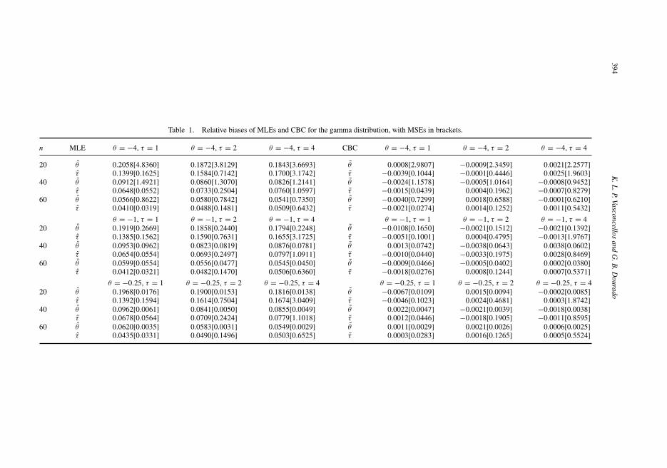
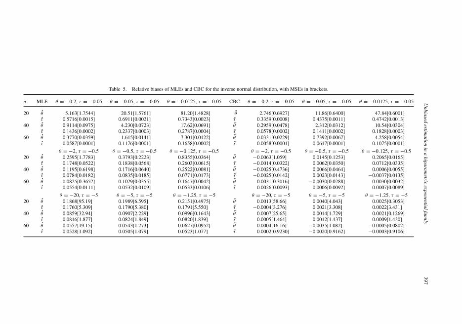
For each specific distribution, we present two large tables. The first table shows the resultsfor the estimators labeled, respectively, as MLE, and CBC, the corrective bias correction,defined in equation (9). The second large table shows the results for the estimators labeled,respectively, as PBC obtained by maximizing equation (12), and BBC. In each very specificsituation (distribution, estimator, parameter values and sample size), we provide the relativebias estimated from the 10,000 replications, with the corresponding estimated mean squareerror (MSE) in brackets. The relative bias for a given estimator of a given parameter α is hereestimated as (α − α)/α, where α is the average value (sample mean) of the 10,000 estimatesof the true parameter α in the study (α = θ or α = τ ). The MSE is estimated in a similarfashion by adding the sample variance of the 10,000 estimates to the square of the estimatedbias.

Two additional tables are also presented for each distribution. The first gives, for each samplesize and estimator, the quantity we define as integrated relative bias square norm (IRBSQ).This quantity is also used in Cribari-Neto and Vasconcellos [9] and is defined here for eachspecific estimator and sample size as

IRBSQ =√√√√1

9

9∑h=1

(rh)2,

where the rh’s correspond to the nine different values of the relative bias estimated for thenine different situations for the parameter vector (θ , τ ). This can provide an idea of the meanbehavior of the relative bias considering the different possible values of the parameter vector.

Associated with the last quantity, we also present, in the last table, the average relative meansquare error (ARMSE) given for each specific estimator and sample size as

ARMSE = 1

9

3∑k=1

3∑h=1

MSEh,k

α2h

,

where the MSEh,k’s correspond to the nine possible situations studied here for the parametervalues, and α1, α2, α3 are the three different values considered for the parameter α in the study(α = θ or α = τ ). This quantity, also used in Cribari-Neto and Vasconcellos [9], will providean idea of the mean behavior of the MSE.

We present below the simulation results for each of the three distributions studied here.

Unbiased estimation in a biparametric exponential family 393

4.1 Gamma distribution

The gamma distribution is probably the most well-known and used of the three distributionsstudied here. After a convenient reparameterization, it is seen that this distribution admits adensity in (0, ∞) in the form of equation (1), with b(x) = x−1, T (x) = log x and ρ(θ, τ ) =τ log(−θ−1) + log (τ), where θ < 0, τ > 0 and (·) stands for the well-known gammafunction. Using equations (6) and (7) in section 3, we will obtain, for this particular case,

B(θ) = θ(2τψ ′(τ ) − 3)ψ ′(τ ) − τψ ′′(τ )

2n(τψ ′(τ ) − 1)2and B(τ ) = 2 − τψ ′(τ ) + τ 2ψ ′′(τ )

2n(τψ ′(τ ) − 1)2,

where ψ(·) is the digamma function (first derivative of the log of the gamma function), theprimes representing differentiation with respect to the argument.

Also, the modified log-likelihood in equation (12) can be easily obtained, the D quantity inequation (8) being given by

D = τψ ′(τ ) − 1

θ2.

Simulation results for this distribution are presented in tables 1–4. In the simulations, wehave considered three different values for the configuration parameter τ of the distribution(including τ = 1, which corresponds to the exponential distribution), as well as three differentvalues for the coefficient of variation.

From the tables, it is seen that all corrections are effective in reducing the relative bias of theoriginal MLE. We observe that the analytical bias corrections (the corrective and preventivemethods) are the most effective, showing better performance than the bootstrap scheme. Forsmall values of the sample size, in particular, we can see that the analytical corrections performmuch better. When n = 60, all three corrections show similar performance, but still better thanthe MLE. Also, an interesting feature we can observe in tables 1 and 2 is that, in general, bothanalytically corrected estimates lie in the same side of the true value of the parameter. That is,in general, both corrections underestimate the true value of the parameter (and, hence, bothrelative biases are negative) or both corrections overestimate the true value (and, hence, bothrelative biases are positive).

Also, all three corrections show very similar performance in terms of MSE, always reducingthe MSE of the original MLE. Therefore, we can conclude that the analytical bias correctionsperform better in terms of reducing bias, but the numerical BBC is as effective in terms of MSE.

4.2 Inverse Gaussian distribution

The inverse normal or inverse Gaussian distribution has been widely studied in the literature[24, 25]. In particular, it has been shown very useful to model the probabilities of first passagetime in the Brownian motion, if the distance covered in unit time is assumed normal. Becauseof the inverse relation that can be established between the cumulant generating functions of thetime to cover a unit distance and the distance covered in unit time, the distribution is referredto as inverse Gaussian or inverse normal.

This distribution admits a density in (0, ∞) in the form of equation (1), with b(x) =(2πx3)−1/2, T (x) = x−1 and ρ(θ, τ ) = −2

√θτ − (1/2) log(−2τ), where θ < 0 and τ < 0.

Unlike the other two distributions studied here, the MLEs of the parameters in this case can beobtained in closed form. Keeping in mind that θ < 0 and τ < 0, we can immediately obtain

394K

.L.P.Vasconcellos

andG

.B.D

ourado

Table 1. Relative biases of MLEs and CBC for the gamma distribution, with MSEs in brackets.

n MLE θ = −4, τ = 1 θ = −4, τ = 2 θ = −4, τ = 4 CBC θ = −4, τ = 1 θ = −4, τ = 2 θ = −4, τ = 4

20 θ 0.2058[4.8360] 0.1872[3.8129] 0.1843[3.6693] θ 0.0008[2.9807] −0.0009[2.3459] 0.0021[2.2577]τ 0.1399[0.1625] 0.1584[0.7142] 0.1700[3.1742] τ −0.0039[0.1044] −0.0001[0.4446] 0.0025[1.9603]

40 θ 0.0912[1.4921] 0.0860[1.3070] 0.0826[1.2141] θ −0.0024[1.1578] −0.0005[1.0164] −0.0008[0.9452]τ 0.0648[0.0552] 0.0733[0.2504] 0.0760[1.0597] τ −0.0015[0.0439] 0.0004[0.1962] −0.0007[0.8279]

60 θ 0.0566[0.8622] 0.0580[0.7842] 0.0541[0.7350] θ −0.0040[0.7299] 0.0018[0.6588] −0.0001[0.6210]τ 0.0410[0.0319] 0.0488[0.1481] 0.0509[0.6432] τ −0.0021[0.0274] 0.0014[0.1252] 0.0011[0.5432]

θ = −1, τ = 1 θ = −1, τ = 2 θ = −1, τ = 4 θ = −1, τ = 1 θ = −1, τ = 2 θ = −1, τ = 420 θ 0.1919[0.2669] 0.1858[0.2440] 0.1794[0.2248] θ −0.0108[0.1650] −0.0021[0.1512] −0.0021[0.1392]

τ 0.1385[0.1562] 0.1590[0.7631] 0.1655[3.1725] τ −0.0051[0.1001] 0.0004[0.4795] −0.0013[1.9767]40 θ 0.0953[0.0962] 0.0823[0.0819] 0.0876[0.0781] θ 0.0013[0.0742] −0.0038[0.0643] 0.0038[0.0602]

τ 0.0654[0.0554] 0.0693[0.2497] 0.0797[1.0911] τ −0.0010[0.0440] −0.0033[0.1975] 0.0028[0.8469]60 θ 0.0599[0.0554] 0.0556[0.0477] 0.0545[0.0450] θ −0.0009[0.0466] −0.0005[0.0402] 0.0002[0.0380]

τ 0.0412[0.0321] 0.0482[0.1470] 0.0506[0.6360] τ −0.0018[0.0276] 0.0008[0.1244] 0.0007[0.5371]

θ = −0.25, τ = 1 θ = −0.25, τ = 2 θ = −0.25, τ = 4 θ = −0.25, τ = 1 θ = −0.25, τ = 2 θ = −0.25, τ = 420 θ 0.1968[0.0176] 0.1900[0.0153] 0.1816[0.0138] θ −0.0067[0.0109] 0.0015[0.0094] −0.0002[0.0085]

τ 0.1392[0.1594] 0.1614[0.7504] 0.1674[3.0409] τ −0.0046[0.1023] 0.0024[0.4681] 0.0003[1.8742]40 θ 0.0962[0.0061] 0.0841[0.0050] 0.0855[0.0049] θ 0.0022[0.0047] −0.0021[0.0039] −0.0018[0.0038]

τ 0.0678[0.0564] 0.0709[0.2424] 0.0779[1.1018] τ 0.0012[0.0446] −0.0018[0.1905] −0.0011[0.8595]60 θ 0.0620[0.0035] 0.0583[0.0031] 0.0549[0.0029] θ 0.0011[0.0029] 0.0021[0.0026] 0.0006[0.0025]

τ 0.0435[0.0331] 0.0490[0.1496] 0.0503[0.6525] τ 0.0003[0.0283] 0.0016[0.1265] 0.0005[0.5524]

Unbiased

estimation

ina

biparametric

exponentialfamily

395

Table 2. Relative biases of PBC and BBC estimates for the gamma distribution, with MSEs in brackets.

n PBC θ = −4, τ = 1 θ = −4, τ = 2 θ = −4, τ = 4 BBC θ = −4, τ = 1 θ = −4, τ = 2 θ = −4, τ = 4

20 θ∗ −0.0002[2.9796] −0.0013[2.3451] 0.0018[2.2573] θ −0.0290[2.9906] −0.0277[2.3756] −0.0241[2.2647]τ ∗ −0.0049[0.1044] −0.0006[0.4445] 0.0022[1.9601] τ −0.0241[0.1041] −0.0232[0.4469] −0.0215[1.9704]

40 θ∗ −0.0026[1.1577] −0.0006[1.0163] −0.0009[0.9451] θ −0.0068[1.1580] −0.0040[1.0217] −0.0046[0.9467]τ ∗ −0.0018[0.0439] 0.0003[0.1962] −0.0008[0.8279] τ −0.0045[0.0439] −0.0026[0.1969] −0.0041[0.8311]

60 θ∗ −0.0041[0.7299] 0.0018[0.6588] −0.0002[0.6210] θ −0.0053[0.7345] 0.0002[0.6609] −0.0014[0.6234]τ ∗ −0.0022[0.0274] 0.0013[0.1252] 0.0010[0.5432] τ −0.0030[0.0275] −0.0001[0.1256] −0.0001[0.5452]

θ = −1, τ = 1 θ = −1, τ = 2 θ = −1, τ = 4 θ = −1, τ = 1 θ = −1, τ = 2 θ = −1, τ = 420 θ∗ −0.0119[0.1650] −0.0026[0.1512] −0.0024[0.1391] θ −0.0397[0.1656] −0.0298[0.1503] −0.0289[0.1398]

τ ∗ −0.0061[0.1002] −0.0001[0.4794] −0.0016[1.9764] τ −0.0252[0.0992] −0.0222[0.4779] −0.0260[1.9792]40 θ∗ 0.0011[0.0742] −0.0039[0.0643] 0.0037[0.0602] θ −0.0027[0.0742] −0.0079[0.0644] 0.0000[0.0605]

τ ∗ −0.0012[0.0440] −0.0034[0.1975] 0.0027[0.8469] τ −0.0037[0.0440] −0.0069[0.1977] −0.0008[0.8506]60 θ∗ −0.0010[0.0466] −0.0005[0.0402] 0.0002[0.0380] θ −0.0025[0.0468] −0.0022[0.0402] −0.0013[0.0380]

τ ∗ −0.0019[0.0276] 0.0008[0.1244] 0.0007[0.5371] τ −0.0031[0.0276] −0.0007[0.1247] −0.0007[0.5374]

θ = −0.25, τ = 1 θ = −0.25, τ = 2 θ = −0.25, τ = 4 θ = −0.25, τ = 1 θ = −0.25, τ = 2 θ = −0.25, τ = 420 θ∗ −0.0078[0.0109] 0.0010[0.0094] −0.0005[0.0085] θ −0.0349[0.0109] −0.0250[0.0095] −0.0258[0.0085]

τ ∗ −0.0056[0.1024] 0.0019[0.4680] 0.0000[1.8740] τ −0.0237[0.1017] −0.0196[0.4723] −0.0233[1.8878]40 θ∗ 0.0019[0.0047] −0.0023[0.0039] 0.0017[0.0038] θ −0.0018[0.0047] −0.0061[0.0039] −0.0024[0.0038]

τ ∗ 0.0010[0.0446] −0.0019[0.1905] −0.0010[0.8599] τ −0.0015[0.0447] −0.0050[0.1911] −0.0028[0.8595]60 θ∗ 0.0010[0.0029] 0.0020[0.0026] 0.0006[0.0025] θ −0.0004[0.0029] 0.0003[0.0026] −0.0004[0.0025]

τ ∗ 0.0002[0.0283] 0.0016[0.1265] 0.0005[0.5524] τ −0.0007[0.0284] 0.0003[0.1269] −0.0005[0.5552]

396 K. L. P. Vasconcellos and G. B. Dourado

Table 3. IRBSQ for gamma estimation.

MLE CBC PBC BBC

n = 20 θ 0.1894 0.0045 0.0050 0.0298τ 0.1559 0.0029 0.0034 0.0233

n = 40 θ 0.0833 0.0024 0.0024 0.0047τ 0.0719 0.0018 0.0018 0.0040

n = 60 θ 0.0572 0.0017 0.0017 0.0022τ 0.0472 0.0013 0.0013 0.0015

Table 4. ARMSE for gamma estimation.

MLE CBC PBC BBC

n = 20 θ 0.2503 0.1545 0.1544 0.1550τ 0.1802 0.1131 0.1131 0.1132

n = 40 θ 0.1394 0.0658 0.0658 0.0659τ 0.0618 0.0485 0.0486 0.0487

n = 60 θ 0.0499 0.0420 0.0420 0.0421τ 0.0366 0.0310 0.0310 0.0311

the derivatives:

ρ(1,0) =√

τ

θand ρ(1,0) =

√θ

τ− 1

2τ.

From the derivatives above and (3), we obtain the MLEs

τ = 1

2

⎡⎣(

1

n

n∑i=1

Xi

)−1

− 1

n

n∑i=1

(Xi)−1

⎤⎦

−1

and θ = τ

((1/n)∑n

i=1 Xi)2.

Using equations (6) and (7) of the last section, the second-order biases of the MLEs can beeasily obtained.

B(θ) = 3(1 + 2√

θτ)

2n

√θ

τ

and

B(τ ) = 3τ/n.

The PBC can be easily calculated by maximizing the modified log-likelihood inequation (12), the D quantity in equation (8) being given by

D = 1

4(θτ )−3/2.

Simulation results for this distribution are presented in tables 5–8. The idea was to considerthree different values for the mean of the distribution (0.5, 1 and 2). Also, since both second-order biases depend on τ , we have considered three very different values for this parameter.

From the tables, we observe that all corrections are effective in reducing the relative biasand MSE of the original MLE. Furthermore, the three corrections behave quite similarly forthis distribution, both in terms of bias and MSE, with Firth’s correction showing a very slightlybetter performance overall. We also can see, in tables 5 and 6, that, again, in general, bothanalytically corrected estimates lie at the same side of the true value of the parameter.

Therefore, for this case, there is not much difference between the three corrections, both interms of bias and MSE, the three of them showing better performance than the original MLE.

Unbiased

estimation

ina

biparametric

exponentialfamily

397

Table 5. Relative biases of MLEs and CBC for the inverse normal distribution, with MSEs in brackets.

n MLE θ = −0.2, τ = −0.05 θ = −0.05, τ = −0.05 θ = −0.0125, τ = −0.05 CBC θ = −0.2, τ = −0.05 θ = −0.05, τ = −0.05 θ = −0.0125, τ = −0.05

20 θ 5.163[1.7544] 20.51[1.5761] 81.20[1.4828] θ 2.746[0.6927] 11.86[0.6400] 47.84[0.6001]τ 0.5716[0.0015] 0.6911[0.0021] 0.7343[0.0023] τ 0.3359[0.0008] 0.4375[0.0011] 0.4742[0.0013]

40 θ 0.9114[0.0975] 4.230[0.0723] 17.62[0.0691] θ 0.2959[0.0478] 2.312[0.0312] 10.54[0.0304]τ 0.1436[0.0002] 0.2337[0.0003] 0.2787[0.0004] τ 0.0578[0.0002] 0.1411[0.0002] 0.1828[0.0003]

60 θ 0.3770[0.0359] 1.615[0.0141] 7.301[0.0122] θ 0.0331[0.0229] 0.7392[0.0067] 4.258[0.0054]τ 0.0587[0.0001] 0.1176[0.0001] 0.1658[0.0002] τ 0.0058[0.0001] 0.0617[0.0001] 0.1075[0.0001]

θ = −2, τ = −0.5 θ = −0.5, τ = −0.5 θ = −0.125, τ = −0.5 θ = −2, τ = −0.5 θ = −0.5, τ = −0.5 θ = −0.125, τ = −0.520 θ 0.2595[1.7783] 0.3793[0.2223] 0.8355[0.0364] θ −0.0063[1.059] 0.0145[0.1253] 0.2065[0.0165]

τ 0.1748[0.0522] 0.1838[0.0568] 0.2603[0.0615] τ −0.0014[0.0322] 0.0062[0.0350] 0.0712[0.0335]40 θ 0.1195[0.6198] 0.1716[0.0640] 0.2522[0.0081] θ −0.0025[0.4736] 0.0066[0.0464] 0.0006[0.0055]

τ 0.0784[0.0182] 0.0835[0.0185] 0.0771[0.0173] τ −0.0025[0.0142] 0.0023[0.0143] −0.0037[0.0135]60 θ 0.0825[0.3652] 0.1029[0.0355] 0.1647[0.0042] θ 0.0031[0.3016] −0.0030[0.0288] 0.0030[0.0032]

τ 0.0554[0.0111] 0.0532[0.0109] 0.0533[0.0106] τ 0.0026[0.0093] 0.0006[0.0092] 0.0007[0.0089]

θ = −20, τ = −5 θ = −5, τ = −5 θ = −1.25, τ = −5 θ = −20, τ = −5 θ = −5, τ = −5 θ = −1.25, τ = −520 θ 0.1868[95.19] 0.1989[6.595] 0.2151[0.4975] θ 0.0013[58.66] 0.0040[4.043] 0.0025[0.3053]

τ 0.1760[5.309] 0.1790[5.380] 0.1791[5.550] τ −0.0004[3.276] 0.0021[3.308] 0.0022[3.431]40 θ 0.0859[32.94] 0.0907[2.229] 0.0996[0.1643] θ 0.0007[25.65] 0.0014[1.729] 0.0021[0.1269]

τ 0.0816[1.877] 0.0824[1.849] 0.0820[1.839] τ 0.0005[1.464] 0.0012[1.437] 0.0009[1.430]60 θ 0.0557[19.15] 0.0543[1.273] 0.0627[0.0952] θ 0.0004[16.16] −0.0035[1.082] −0.0005[0.0802]

τ 0.0528[1.092] 0.0505[1.079] 0.0523[1.077] τ 0.0002[0.9230] −0.0020[0.9162] −0.0003[0.9106]

398K

.L.P.Vasconcellos

andG

.B.D

ourado

Table 6. Relative biases of PBC and BBC estimates for the inverse normal distribution, with MSEs in brackets.

n PBC θ = −0.2, τ = −0.05 θ = −0.05, τ = −0.05 θ = −0.0125, τ = −0.05 BBC θ = −0.2, τ = −0.05 θ = −0.05, τ = −0.05 θ = −0.0125, τ = −0.05

20 θ∗ 2.429[0.6310] 10.65[0.5739] 43.10[0.5340] θ 2.354[0.7201] 10.25[0.6210] 42.39[0.6083]τ ∗ 0.3025[0.0007] 0.3988[0.0010] 0.4336[0.0011] τ 0.3083[0.0008] 0.4080[0.0011] 0.4449[0.0012]

40 θ∗ 0.2208[0.0471] 2.012[0.0284] 9.345[0.0270] θ 0.2561[0.0521] 2.178[0.0339] 10.24[0.0328]τ ∗ 0.0464[0.0002] 0.1254[0.0002] 0.1653[0.0003] τ 0.0567[0.0002] 0.1398[0.0002] 0.1821[0.0003]

60 θ∗ 0.0048[0.0231] 0.6114[0.0064] 3.737[0.0049] θ 0.0237[0.0243] 0.7182[0.0074] 4.163[0.0059]τ ∗ 0.0010[0.0001] 0.0528[0.0001] 0.0967[0.0001] τ 0.0058[0.0001] 0.0627[0.0001] 0.1081[0.0001]

θ = −2, τ = −0.5 θ = −0.5, τ = −0.5 θ = −0.125, τ = −0.5 θ = −2, τ = −0.5 θ = −0.5, τ = −0.5 θ = −0.125, τ = −0.520 θ∗ −0.0117[1.060] −0.0021[0.1257] 0.1455[0.0164] θ −0.0415[1.075] −0.0381[0.1306] 0.1065[0.0177]

τ ∗ −0.0051[0.0323] −0.0022[0.0351] 0.0516[0.0331] τ −0.0242[0.0325] −0.0155[0.0353] 0.0480[0.0330]40 θ∗ −0.0037[0.4737] 0.0033[0.0464] −0.0106[0.0055] θ −0.0071[0.4734] −0.0003[0.0466] −0.0093[0.0057]

τ ∗ −0.0033[0.0142] 0.0006[0.0143] −0.0074[0.0135] τ −0.0059[0.0143] −0.0010[0.0143] −0.0062[0.0135]60 θ∗ 0.0026[0.3016] −0.0044[0.0288] −0.0015[0.0032] θ 0.0014[0.3014] −0.0044[0.0289] 0.0013[0.0032]

τ ∗ 0.0023[0.0093] −0.0001[0.0092] −0.0008[0.0089] τ 0.0015[0.0093] −0.0002[0.0092] 0.0001[0.0089]

θ = −20, τ = −5 θ = −5, τ = −5 θ = −1.25, τ = −5 θ = −20, τ = −5 θ = −5, τ = −5 θ = −1.25, τ = −520 θ∗ 0.0009[58.66] 0.0032[4.043] 0.0009[0.3053] θ −0.0240[59.03] −0.0219[4.086] −0.0271[0.3073]

τ ∗ −0.0007[3.276] 0.0015[3.308] 0.0008[3.431] τ −0.0245[3.292] −0.0215[3.362] −0.0221[3.457]40 θ∗ 0.0006[25.65] 0.0012[1.729] 0.0017[0.1269] θ −0.0033[25.75] −0.0026[1.741] −0.0021[0.1276]

τ ∗ 0.0004[1.464] 0.0011[1.437] 0.0006[1.430] τ −0.0035[1.470] −0.0024[1.448] −0.0027[1.437]60 θ∗ 0.0004[16.16] −0.0035[1.082] −0.0006[0.0802] θ −0.0012[16.21] −0.0052[1.086] −0.0022[0.0807]

τ ∗ 0.0001[0.9230] −0.0021[0.9163] −0.0004[0.9107] τ −0.0013[0.9257] −0.0036[0.9192] −0.0018[0.9159]

Unbiased estimation in a biparametric exponential family 399

Table 7. IRBSQ for inverse normal estimation.

MLE CBC PBC BBC

n = 20 θ 27.97 16.45 14.82 14.56τ 0.4178 0.2436 0.2214 0.2271

n = 40 θ 6.049 3.598 3.187 3.491τ 0.1461 0.0794 0.0709 0.0789

n = 60 θ 2.497 1.441 1.262 1.408τ 0.0827 0.0414 0.0367 0.0417

Table 8. ARMSE for inverse normal estimation.

MLE CBC PBC BBC

n = 20 θ 12.12 7.349 7.327 7.400τ 1.824 1.124 1.124 1.135

n = 40 θ 4.029 3.127 3.126 3.140τ 0.6245 0.4859 0.4859 0.4887

n = 60 θ 2.332 1.966 1.966 1.972τ 0.3647 0.3086 0.3086 0.3098

4.3 Log-beta distribution

This is the distribution of X = − log Y when Y is beta distributed. This distribution has alsobeen already studied in the literature. It is mentioned in Johnson et al., [26], where expressionsfor cumulants can be found. Florens et al., [27], have considered it as the distribution of thehazard function in Bayesian duration studies for which a beta prior distribution is assigned toa given probability. Jones [28] has also argued that this distribution can be useful for lifetimemodels. Dufresne [29] has obtained some approximation theorems in a family that generalizesthis distribution.Additionally, Hu et al., [30], suggest it as a good choice for statistical modelingin some genetic studies.

This distribution admits a density in (0, ∞) in the form of (1), with b(x) = (1 − e−x)−1,T (x) = log(1 − e−x) and ρ(θ, τ ) = log (τ) + log (−θ) − log (τ − θ), where θ < 0and τ > 0. The MLEs of the parameters in this case can be obtained by numerical opti-mization. Also, from equations (6) and (7) of the last section, the second-order biases of theMLEs can be obtained as

B(θ) = N(θ)

2nD2 and B(τ ) = N(τ )

2nD2 ,

where

N(θ) = ψ ′(τ − θ)(ψ ′(−θ)ψ ′′(τ ) − 2ψ ′′(−θ)ψ ′(τ )) + (ψ ′(τ − θ))2(ψ ′′(−θ) − ψ ′′(τ ))

+ (ψ ′(τ ))2(ψ ′′(−θ) − ψ ′′(τ − θ)) − ψ ′′(τ − θ)ψ ′(−θ)ψ ′(τ ),

N(τ ) = ψ ′(τ − θ)(ψ ′(τ )ψ ′′(−θ) − 2ψ ′′(τ )ψ ′(−θ)) + (ψ ′(τ − θ))2(ψ ′′(τ ) − ψ ′′(−θ))

+ (ψ ′(−θ))2(ψ ′′(τ ) − ψ ′′(τ − θ)) − ψ ′′(τ − θ)ψ ′(−θ)ψ ′(τ )

and

D = ψ ′(τ − θ)(ψ ′(−θ) + ψ ′(τ )) − ψ ′(−θ)ψ ′(τ ).

The PBC estimates can be easily calculated by maximizing the modified log-likelihood inequation (12), with the D quantity being given above.

400K

.L.P.Vasconcellos

andG

.B.D

ourado

Table 9. Relative biases of MLEs and CBC for the log-beta distribution, with MSEs in brackets.

n MLE θ = −0.5, τ = 1 θ = −0.5, τ = 3 θ = −0.5, τ = 10 CBC θ = −0.5, τ = 1 θ = −0.5, τ = 3 θ = −5, τ = 10

20 θ 0.1279[0.0349] 0.1279[0.0329] 0.1346[0.0343] θ −0.0006[0.0228] 0.0016[0.0216] 0.0074[0.0223]τ 0.1762[0.2398] 0.2170[3.0061] 0.2536[40.90] τ −0.0008[0.1446] −0.0035[1.771] 0.0100[23.75]

40 θ 0.0569[0.0126] 0.0539[0.0117] 0.0595[0.0119] θ −0.0022[0.0102] −0.0041[0.0095] 0.0011[0.0096]τ 0.0808[0.0768] 0.0936[0.9603] 0.1107[12.36] τ 0.0003[0.0589] −0.0063[0.738] 0.0009[9.278]

60 θ 0.0385[0.0075] 0.0402[0.0074] 0.0376[0.0070] θ 0.0000[0.0065] 0.0022[0.0064] −0.0003[0.0061]τ 0.0529[0.0455] 0.0691[0.5659] 0.0699[7.115] τ 0.0009[0.0380] 0.0039[0.4635] −0.0010[5.877]

θ = −1, τ = 1 θ = −1, τ = 3 θ = −1, τ = 10 θ = −1, τ = 1 θ = −1, τ = 3 θ = −5, τ = 1020 θ 0.1509[0.1794] 0.1475[0.1686] 0.1419[0.1554] θ −0.0018[0.1130] 0.0018[0.1071] −0.0023[0.0988]

τ 0.1517[0.1765] 0.1820[2.180] 0.1975[26.63] τ −0.0012[0.1107] −0.0009[1.346] −0.0002[16.28]40 θ 0.0701[0.0612] 0.0698[0.0564] 0.0656[0.0554] θ 0.0000[0.0482] 0.0028[0.0443] −0.0008[0.0440]

τ 0.0715[0.0617] 0.0898[0.7368] 0.0881[8.965] τ 0.0001[0.0484] 0.0055[0.5654] −0.0023[6.972]60 θ 0.0457[0.0369] 0.0428[0.0325] 0.0415[0.0319] θ 0.0002[0.0314] −0.0006[0.0278] −0.0016[0.0273]

τ 0.0468[0.0364] 0.0549[0.4209] 0.0585[5.140] τ 0.0012[0.0309] 0.0005[0.3540] −0.0003[4.315]

θ = −5, τ = 1 θ = −5, τ = 3 θ = −5, τ = 10 θ = −5, τ = 1 θ = −5, τ = 3 θ = −5, τ = 1020 θ 0.1975[6.722] 0.1645[4.934] 0.1634[4.757] θ 0.0053[4.111] −0.0073[3.075] −0.0051[2.956]

τ 0.1457[0.1652] 0.1624[1.692] 0.1695[20.06] τ 0.0008[0.1050] −0.0026[1.051] −0.0050[12.42]40 θ 0.0901[2.167] 0.0809[1.744] 0.0753[1.727] θ 0.0023[1.672] 0.0012[1.352] −0.0024[1.357]

τ 0.0687[0.0564] 0.0771[0.5894] 0.0781[7.246] τ 0.0020[0.0445] 0.0010[0.4587] −0.0022[5.678]60 θ 0.0572[1.219] 0.0525[1.066] 0.0530[0.9933] θ 0.0004[1.022] 0.0008[0.8993] 0.0023[0.8333]

τ 0.0437[0.0320] 0.0507[0.3565] 0.0542[4.195] τ 0.0005[0.0272] 0.0013[0.3010] 0.0018[3.521]

Unbiased

estimation

ina

biparametric

exponentialfamily

401

Table 10. Relative biases of PBC and BBC estimates for the log-beta distribution, with MSEs in brackets.

n PBC θ = −0.5, τ = 1 θ = −0.5, τ = 3 θ = −0.5, τ = 10 BBC θ = −0.5, τ = 1 θ = −0.5, τ = 3 θ = −0.5, τ = 10

20 θ∗ −0.0012[0.0228] −0.0005[0.0216] 0.0048[0.0223] θ −0.0186[0.0227] −0.0145[0.0215] −0.0082[0.0219]τ ∗ −0.0002[0.1442] −0.0050[1.764] 0.0072[23.69] τ −0.0315[0.1466] −0.0385[1.837] −0.0294[24.27]

40 θ∗ −0.0023[0.0102] −0.0046[0.0095] 0.0005[0.0096] θ −0.0046[0.0103] −0.0065[0.0095] −0.0008[0.0097]τ ∗ 0.0005[0.0589] −0.0066[0.7332] 0.0003[9.273] τ −0.0038[0.0591] −0.0115[0.7374] −0.0036[9.348]

60 θ∗ −0.0001[0.0065] 0.0020[0.0064] −0.0006[0.0061] θ −0.0010[0.0065] 0.0015[0.0064] −0.0011[0.0061]τ ∗ 0.0010[0.0380] 0.0038[0.4633] −0.0013[5.876] τ −0.0005[0.0383] 0.0023[0.4665] −0.0029[5.895]

θ = −1, τ = 1 θ = −1, τ = 3 θ = −1, τ = 10 θ = −1, τ = 1 θ = −1, τ = 3 θ = −1, τ = 1020 θ∗ −0.0017[0.1129] 0.0011[0.1070] −0.0032[0.0989] θ −0.0238[0.1132] −0.0182[0.1062] −0.0216[0.0983]

τ ∗ −0.0010[0.1106] −0.0014[1.345] −0.0012[16.27] τ −0.0224[0.1115] −0.0265[1.353] −0.0275[16.30]40 θ∗ 0.0000[0.0482] 0.0026[0.0443] −0.0010[0.0440] θ −0.0037[0.0484] 0.0001[0.0442] −0.0042[0.0438]

τ ∗ 0.0012[0.0484] 0.0054[0.5652] −0.0025[6.971] τ −0.0023[0.0488] 0.0021[0.5669] −0.0069[6.965]60 θ∗ 0.0002[0.0314] −0.0006[0.0278] −0.0017[0.0273] θ −0.0010[0.0315] −0.0017[0.0279] −0.0029[0.0274]

τ ∗ 0.0012[0.0309] 0.0004[0.3540] −0.0004[4.314] τ 0.0000[0.0309] −0.0010[0.3548] −0.0021[4.327]

θ = −5, τ = 1 θ = −5, τ = 3 θ = −5, τ = 10 θ = −5, τ = 1 θ = −5, τ = 3 θ = −5, τ = 1020 θ∗ 0.0045[4.107] −0.0076[3.073] −0.0054[2.956] θ −0.0223[4.091] −0.0316[3.095] −0.0287[2.982]

τ ∗ −0.0001[0.1051] −0.0029[1.051] −0.0052[12.41] τ −0.0189[0.1046] −0.0259[1.050] −0.0297[12.56]40 θ∗ 0.0022[1.671] 0.0012[1.352] −0.0025[1.357] θ −0.0015[1.675] −0.0022[1.360] −0.0067[1.360]

τ ∗ 0.0018[0.0445] 0.0009[0.4586] −0.0023[5.677] τ −0.0008[0.0445] −0.0024[0.4609] −0.0066[5.696]60 θ∗ 0.0003[1.022] 0.0008[0.8993] 0.0023[0.8333] θ −0.0011[1.028] −0.0007[0.9016] 0.0009[0.8356]

τ ∗ 0.0004[0.0272] 0.0012[0.3010] 0.0018[3.521] τ −0.0006[0.0274] −0.0001[0.3016] 0.0003[3.529]

402 K. L. P. Vasconcellos and G. B. Dourado

Table 11. IRBSQ for log-beta estimation.

MLE CBC PBC BBC

n = 20 θ 0.1521 0.0044 0.0040 0.0977τ 0.1868 0.0040 0.0036 0.0283

n = 40 θ 0.0653 0.0022 0.0023 0.0040

τ 0.2432 0.0031 0.0032 0.0054

n = 60 θ 0.0459 0.0012 0.0012 0.0015

τ 0.0563 0.0016 0.0016 0.0015

Table 12. ARMSE for log-beta estimation.

MLE CBC PBC BBC

n = 20 θ 0.1743 0.1102 0.1101 0.1099τ 0.2468 0.1498 0.1495 0.1517

n = 40 θ 0.0604 0.0477 0.0477 0.0478

τ 0.0816 0.0629 0.0629 0.0632

n = 60 θ 0.0356 0.0303 0.0303 0.0304

τ 0.0475 0.0397 0.0397 0.0399

Simulation results for this distribution are presented in tables 9–12. We have chosen threedifferent values for each parameter, which gives nine different cases corresponding to threeexponential distributions (the cases corresponding to τ = 1) and six very different shapes forthe density of the distribution (the cases corresponding to the last two columns).

The tables indicate that, for this distribution, all three corrections reduce the relative bias andMSE of the original MLE. In particular, the two analytical corrections are the most effectivein reducing relative bias when the sample size is small (20 or 40 observations). For n = 60,all three estimators have similar performances in terms of bias reduction. On the other hand,all three corrections show similar performances in terms of MSEs, for all the values of theparameters studied here. Also, we observe, from tables 9 and 10, that, in many situations, thetwo analytically corrected estimates lie on the same side of the true value. In other words,their biases have the same sign for many situations.

The conclusions for this distribution are, therefore, the same conclusions obtained for thegamma distribution.

5. Conclusions

In this work, we have focused our attention on the biparametric exponential family proposed byLindsay [13]. We have obtained simple closed-form expressions for the second-order biases ofthe MLE of both parameters.We discussed Firth’s [6] proposal for bias reduction and concludedthat, for the family of distributions here studied, the bias corrected estimator proposed by Firthcan be obtained by maximization of a modified log-likelihood.

Numerical results were obtained for three particular cases: the gamma, the inverse normaland the log-beta distributions.

For the gamma and log-beta distributions, we have come essentially to the same conclusions.All three bias reduction schemes here studied (the direct correction, Firth’s proposal and thebootstrap method) are successful in reducing the bias of the original MLE, the first twocorrections (the analytical ones) showing better performance than the numerical bootstrap

Unbiased estimation in a biparametric exponential family 403

correction in terms of relative bias. In addition, all three corrected estimators show similarbehavior in terms of MSE, all of them reducing the MSE of the original MLE.

For the inverse normal distribution, all three corrected estimators perform better than theoriginal MLE estimator and all of them show similar performance both in terms of bias andMSE. In other words, although the BBC is not as good as the analytical corrections for thegamma and log-beta distributions, its performance is as good as those of the analytical correc-tions for the inverse normal distribution. Coincidentally or not, the inverse normal distributionis here the case where the MLEs have closed-form expressions. We observe that the boot-strap scheme performed here requires 500 resamplings and the resamplings involve nonlinearmaximizations for the gamma and log-beta distributions. So, this necessity of nonlinear maxi-mization may introduce an extra uncertainty in the BBC, as opposed to the normal inversecase, where the estimates in each resampling can be obtained by closed-form expressions.

Acknowledgements

We gratefully acknowledge the financial support from the Brazilian governmental institutionCNPq. We also would like to thank an anonymous referee for suggestions that led to animproved version of this work.

References

[1] Box, M., 1971, Bias in nonlinear estimation (with discussion). Journal of the Royal Statistical Society B, 33,171–201.

[2] Pike, M., Hill, A. and Smith, P., 1980, Bias and efficiency in logistic analysis of stratified case-control studies.International Journal of Epidemiology, 9, 89–95.

[3] Cook, R., Tsai, C. and Wei, B., 1986, Bias in nonlinear regression. Biometrika, 73, 615–623.[4] Young, D. and Bakir, S., 1987, Bias correction for a generalized log-gamma regression model. Technometrics,

29, 183–191.[5] Cordeiro, G.M. and McCullagh, P., 1991, Bias correction in generalized linear models. Journal of the Royal

Statistical Society B, 53, 629–643.[6] Firth, D., 1993, Bias reduction of maximum likelihood estimates. Biometrika, 80, 27–38.[7] Cordeiro, G.M. and Vasconcellos, K.L.P., 1997, Bias correction for a class of multivariate nonlinear regression

models. Statistics and Probability Letters, 35, 155–164.[8] Cordeiro, G.M. and Vasconcellos, K.L.P., 1999, Second-order biases of the maximum likelihood estimates in

von Mises regression models. Australian and New Zealand Journal of Statistics, 41, 901–910.[9] Cribari–Neto, F. and Vasconcellos, K.L.P., 2002, Nearly unbiased maximum likelihood estimation for the beta

distribution. Journal of Statistical Computation and Simulation, 72, 107–118.[10] Vasconcellos, K.L.P. and Cribari-Neto, F., 2005, Improved maximum likelihood estimation in a new class of

beta regression models. Brazilian Journal of Probability and Statistics, 19, 13–31.[11] Vasconcellos, K.L.P. and Silva, S.G., 2005, Corrected estimates for Student t regression models with unknown

degrees of freedom. Journal of Statistical Computation and Simulation, 75, 409–423.[12] Vasconcellos, K.L.P., Frery, A.C. and Silva, L.B., 2005, Improving estimation in speckled imagery. Computa-

tional Statistics, 20, 503–519.[13] Lindsay, B.G., 1986, Exponential family mixture models. The Annals of Statistics, 14, 124–137.[14] Gelfand, A.E. and Dalal, S.R., 1990, A note on overdispersed exponential families. Biometrika, 77, 55–64.[15] Dey, D.K., Gelfand, A.E. and Pen, F., 1997, Overdispersed generalized linear models. Journal of Statistical

Planning and Inference, 64, 93–107.[16] Cox, D.R. and Hinkley, D., 1974, Theoretical Statistics (London: Chapman and Hall).[17] Lawley, D., 1956, A general method for approximating to the distribution of likelihood ratio criteria. Biometrika,

43, 295–303.[18] Doornik, J.A., 2001, Ox: an Object-oriented Matrix Programming Language (4th ed) London: Timberlake

Consultants and Oxford). Available online at: //www.doornik.com.[19] Fletcher, R., 1987, Practical Methods of Optimization (New York: John Wiley and Sons).[20] Cox, D. and Snell, E., 1968, A general definition of residuals. Journal of the Royal Statistical Society B, 30,

248–275.[21] Wolfram, S., 1991, Mathematica: a System for Doing Mathematics by Computer (Massachusets: Addison-

Wesley).[22] Abell, M.L. and Braselton, J.P., 1994, The Maple V Handbook (New York: AP Professional).[23] Efron, B. and Tibshirani, R.J., 1993, An Introduction to the Bootstrap (New York: Chapman and Hall).

404 K. L. P. Vasconcellos and G. B. Dourado

[24] Chhikara, R.S. and Folks, J.L., 1988, The Inverse Gaussian Distribution (Theory, Methodology and Applications)(New York: Marcel Dekker).

[25] Seshadri, V., 1998, The Inverse Gaussian Distribution: Statistical Theory and Applications (Lecture Notes inStatistics) (Springer).

[26] Johnson, N.L., Kotz, S. and Balakrishnan, N., 1995, Continuous Univariate Distributions, Vol. 2 (New York:John Wiley).

[27] Florens, J.P., Mouchart, M. and Rolin, J.M., 1999, Semi and non parametric Bayesian analysis of durationmodels: a survey. International Statistical Review, 67, 187–210.

[28] Jones, M.C., 2004, Families of distributions arising from distributions of order statistics (with discussion). Test(Sociedad Española de Estádística e Investigación Operativa), 13(1), 1–43.

[29] Dufresne, D., 2005, Fitting combinations of exponentials to probability distributions. Working paper 121,Department of Economics, University of Melbourne, Australia.

[30] Hu, P., Greenwood, C. and Beyene, J., 2005, Integrative analysis of multiple gene expression profileswith quality-adjusted effect size models. BMC:Bioinformatics, 6, 128. Available online at://www.biomedcentral.com/1471-2105/6/128.