Nearly unbiased estimation in a biparametric exponential family
Upload
khangminh22Category
view
3download
0
Hans Petter Langtangen
Finite Diff erence Computing with Exponential Decay Models
Editorial BoardT. J. Barth
M. GriebelD. E. Keyes
R. M. NieminenD. Roose
T. Schlick
110

110
Editors:
Timothy J. BarthMichael GriebelDavid E. KeyesRisto M. NieminenDirk RooseTamar Schlick
Lecture Notesin Computational Scienceand Engineering

More information about this series at http://www.springer.com/series/3527

Hans Petter Langtangen
Finite DifferenceComputing withExponential Decay Models

Hans Petter LangtangenSimula Research LaboratoryLysaker, Norway
On leave from:
Department of InformaticsUniversity of OsloOslo, Norway
ISSN 1439-7358 ISSN 2197-7100 (electronic)Lecture Notes in Computational Science and EngineeringISBN 978-3-319-29438-4 ISBN 978-3-319-29439-1 (eBook)DOI 10.1007/978-3-319-29439-1Springer Cham Heidelberg New York Dordrecht London
Library of Congress Control Number: 2016932614
Mathematic Subject Classification (2010): 34, 65, 68
© The Editor(s) (if applicable) and the Author(s) 2016 This book is published open access.Open Access This book is distributed under the terms of the Creative Commons Attribution-NonCommercial 4.0 International License (http://creativecommons.org/licenses/by-nc/4.0/), whichpermits any noncommercial use, duplication, adaptation, distribution and reproduction in any mediumor format, as long as you give appropriate credit to the original author(s) and the source, a link isprovided to the Creative Commons license and any changes made are indicated.The images or other third party material in this book are included in the work’s Creative Commonslicense, unless indicated otherwise in the credit line; if such material is not included in the work’sCreative Commons license and the respective action is not permitted by statutory regulation, users willneed to obtain permission from the license holder to duplicate, adapt or reproduce the material.This work is subject to copyright. All commercial rights are reserved by the Publisher, whether the wholeor part of the material is concerned, specifically the rights of translation, reprinting, reuse of illustrations,recitation, broadcasting, reproduction on microfilms or in any other physical way, and transmission orinformation storage and retrieval, electronic adaptation, computer software, or by similar or dissimilarmethodology now known or hereafter developed.The use of general descriptive names, registered names, trademarks, service marks, etc. in this publica-tion does not imply, even in the absence of a specific statement, that such names are exempt from therelevant protective laws and regulations and therefore free for general use.The publisher, the authors and the editors are safe to assume that the advice and information in this bookare believed to be true and accurate at the date of publication. Neither the publisher nor the authors orthe editors give a warranty, express or implied, with respect to the material contained herein or for anyerrors or omissions that may have been made.
Printed on acid-free paper
Springer International Publishing AG Switzerland is part of Springer Science+Business Media(www.springer.com)

Preface
This book teaches the basic components in the scientific computing pipeline: mod-eling, differential equations, numerical algorithms, programming, plotting, andsoftware testing. The pedagogical idea is to treat these topics in the context ofa very simple mathematical model, the differential equation for exponential decay,u0.t/ D �au.t/, where u is unknown and a is a given parameter. By keeping themathematical problem simple, the text can go deep into all details about how onemust combine mathematics and computer science to create well-tested, reliable,and flexible software for such a mathematical model.
The writing style is gentle and aims at a broad audience. I am much inspired byNick Trefethen’s praise of easy learning:
Some people think that stiff challenges are the best device to induce learning, but I am notone of them. The natural way to learn something is by spending vast amounts of easy,enjoyable time at it. This goes whether you want to speak German, sight-read at the piano,type, or do mathematics. Give me the German storybook for fifth graders that I feel likereading in bed, not Goethe and a dictionary. The latter will bring rapid progress at first,then exhaustion and failure to resolve.
The main thing to be said for stiff challenges is that inevitably we will encounter them,so we had better learn to face them boldly. Putting them in the curriculum can help teachus to do so. But for teaching the skill or subject matter itself, they are overrated. [13, p. 86]
Prerequisite knowledge for this book is basic one-dimensional calculus andpreferably some experience with computer programming in Python or MATLAB.The material was initially written for self study and therefore features compre-hensive and easy-to-understand explanations. For some readers it may act as anoverview and refresher of traditional mathematical topics and likely a first introduc-tion to many of the software topics. The text can also be used as a case-based andmathematically simple introduction to modern multi-disciplinary problem solvingwith computers, using the range of applications in Chap. 4 as motivation and thentreating the details of the mathematical and computer science subjects from theother chapters. In particular, I have also had in mind the new groups of readersfrom bio- and geo-sciences who need to enter the world of computer-based differ-ential equation modeling, but lack experience with (and perhaps also interest in)mathematics and programming.
The choice of topics in this book is motivated from what is needed in moreadvanced courses on finite difference methods for partial differential equations
v

vi Preface
(PDEs). It turns out that a range of concepts and tools needed for PDEs can beintroduced and illustrated by very simple ordinary differential equation (ODE)examples. The goal of the text is therefore to lay a foundation for understandingnumerical methods for PDEs by first meeting the fundamental ideas in a simplerODE setting. Compared to other books, the present one has a much stronger focuson how to turn mathematics into working code. It also explains the mathematicsand programming in more detail than what is common in the literature.
There is a more advanced companion book in the works, “Finite DifferenceComputing with Partial Differential Equations”, which treats finite difference meth-ods for PDEs using the same writing style and having the same focus on turningmathematical algorithms into reliable software.
Although the main example in the present book is u0 D �au, we also addressthe more general model problem u0 D �a.t/uC b.t/, and the completely general,nonlinear problem u0 D f .u; t/, both for scalar and vector u.t/. The author be-lieves in the principle simplify, understand, and then generalize. That is why westart out with the simple model u0 D �au and try to understand how methods areconstructed, how they work, how they are implemented, and how they may fail forthis problem, before we generalize what we have learned from u0 D �au to morecomplicated models.
The following list of topics will be elaborated on.
� How to think when constructing finite difference methods, with special focus onthe Forward Euler, Backward Euler, and Crank–Nicolson (midpoint) schemes.
� How to formulate a computational algorithm and translate it into Python code.� How to make curve plots of the solutions.� How to compute numerical errors.� How to compute convergence rates.� How to test that an implementation is correct (verification) and how to automate
tests through test functions and unit testing.� How to work with Python concepts such as arrays, lists, dictionaries, lambda
functions, and functions in functions (closures).� How to perform array computing and understand the difference from scalar com-
puting.� How to uncover numerical artifacts in the computed solution.� How to analyze the numerical schemes mathematically to understand why arti-
facts may occur.� How to derive mathematical expressions for various measures of the error in
numerical methods, frequently by using the sympy software for symbolic com-putations.
� How to understand concepts such as finite difference operators, mesh (grid),mesh functions, stability, truncation error, consistency, and convergence.
� How to solve the general nonlinear ODE u0 D f .u; t/, which is either a scalarODE or a system of ODEs (i.e., u and f can either be a function or a vector offunctions).
� How to access professional packages for solving ODEs.� How the model equation u0 D �au arises in a wide range of phenomena in
physics, biology, chemistry, and finance.� How to structure a code in terms of functions.

Preface vii
� How to make reusable modules.� How to read input data flexibly from the command line.� How to create graphical/web user interfaces.� How to use test frameworks for automatic unit testing.� How to refactor code in terms of classes (instead of functions).� How to conduct and automate large-scale numerical experiments.� How to write scientific reports in various formats (LATEX, HTML).
The exposition in a nutshellEverything we cover is put into a practical, hands-on context. All mathematicsis translated into working computing codes, and all the mathematical theory offinite difference methods presented here is motivated from a strong need to un-derstand why we occasionally obtain strange results from the programs. Twofundamental questions saturate the text:
� How do we solve a differential equation problem and produce numbers?� How do we know that the numbers are correct?
Besides answering these two questions, one will learn a lot about mathematicalmodeling in general and the interplay between physics, mathematics, numericalmethods, and computer science.
The book contains a set of exercises in most of the chapters. The exercisesare divided into three categories: exercises refer to the text (usually variations orextensions of examples in the text), problems are stand-alone exercises without ref-erences to the text, and projects are larger problems. Exercises, problems, andprojects share a common numbering to avoid confusion between, e.g., Exercise 4.3and Problem 4.3 (it will be Exercise 4.3 and Problem 4.4 if they follow after eachother).
All program and data files referred to in this book are available from the book’sprimary web site: http://hplgit.github.io/decay-book/doc/web/.
Acknowledgments Professor Svein Linge provided very detailed and constructivefeedback on this text, and all his efforts are highly appreciated. Many students havealso pointed out weaknesses and found errors. A special thank goes to Yapi Dona-tien Achou’s proof reading. Many thanks also to Linda Falch-Koslung, Dr. OlavDajani, and the rest of the OUS team for feeding me with FOLFIRINOX andthereby keeping me alive and in good enough shape to finish this book. As al-ways, the Springer team ensured a smooth and rapid review process and productionphase. This time special thanks go to all the efforts by Martin Peters, Thanh-Ha LeThi, and Yvonne Schlatter.
Oslo, August 2015 Hans Petter Langtangen

Contents
1 Algorithms and Implementations . . . . . . . . . . . . . . . . . . . . . . . 11.1 Finite Difference Methods . . . . . . . . . . . . . . . . . . . . . . . . . 1
1.1.1 A Basic Model for Exponential Decay . . . . . . . . . . . . . 11.1.2 The Forward Euler Scheme . . . . . . . . . . . . . . . . . . . . 21.1.3 The Backward Euler Scheme . . . . . . . . . . . . . . . . . . . 71.1.4 The Crank–Nicolson Scheme . . . . . . . . . . . . . . . . . . . 81.1.5 The Unifying �-Rule . . . . . . . . . . . . . . . . . . . . . . . . 101.1.6 Constant Time Step . . . . . . . . . . . . . . . . . . . . . . . . . 111.1.7 Mathematical Derivation of Finite Difference Formulas . . 111.1.8 Compact Operator Notation for Finite Differences . . . . . . 14
1.2 Implementations . . . . . . . . . . . . . . . . . . . . . . . . . . . . . . . 151.2.1 Computer Language: Python . . . . . . . . . . . . . . . . . . . 161.2.2 Making a Solver Function . . . . . . . . . . . . . . . . . . . . . 171.2.3 Integer Division . . . . . . . . . . . . . . . . . . . . . . . . . . . 181.2.4 Doc Strings . . . . . . . . . . . . . . . . . . . . . . . . . . . . . . 181.2.5 Formatting Numbers . . . . . . . . . . . . . . . . . . . . . . . . 191.2.6 Running the Program . . . . . . . . . . . . . . . . . . . . . . . 201.2.7 Plotting the Solution . . . . . . . . . . . . . . . . . . . . . . . . 211.2.8 Verifying the Implementation . . . . . . . . . . . . . . . . . . 221.2.9 Computing the Numerical Error as a Mesh Function . . . . 251.2.10 Computing the Norm of the Error Mesh Function . . . . . . 261.2.11 Experiments with Computing and Plotting . . . . . . . . . . 281.2.12 Memory-Saving Implementation . . . . . . . . . . . . . . . . 33
1.3 Exercises . . . . . . . . . . . . . . . . . . . . . . . . . . . . . . . . . . . 35
2 Analysis . . . . . . . . . . . . . . . . . . . . . . . . . . . . . . . . . . . . . . . 392.1 Experimental Investigations . . . . . . . . . . . . . . . . . . . . . . . . 39
2.1.1 Discouraging Numerical Solutions . . . . . . . . . . . . . . . 392.1.2 Detailed Experiments . . . . . . . . . . . . . . . . . . . . . . . 41
2.2 Stability . . . . . . . . . . . . . . . . . . . . . . . . . . . . . . . . . . . . 442.2.1 Exact Numerical Solution . . . . . . . . . . . . . . . . . . . . . 442.2.2 Stability Properties Derived from the Amplification Factor 45
ix

x Contents
2.3 Accuracy . . . . . . . . . . . . . . . . . . . . . . . . . . . . . . . . . . . 462.3.1 Visual Comparison of Amplification Factors . . . . . . . . . 462.3.2 Series Expansion of Amplification Factors . . . . . . . . . . 472.3.3 The Ratio of Numerical and Exact Amplification Factors . 492.3.4 The Global Error at a Point . . . . . . . . . . . . . . . . . . . . 502.3.5 Integrated Error . . . . . . . . . . . . . . . . . . . . . . . . . . . 502.3.6 Truncation Error . . . . . . . . . . . . . . . . . . . . . . . . . . 522.3.7 Consistency, Stability, and Convergence . . . . . . . . . . . . 53
2.4 Various Types of Errors in a Differential Equation Model . . . . . . 542.4.1 Model Errors . . . . . . . . . . . . . . . . . . . . . . . . . . . . . 552.4.2 Data Errors . . . . . . . . . . . . . . . . . . . . . . . . . . . . . . 582.4.3 Discretization Errors . . . . . . . . . . . . . . . . . . . . . . . . 612.4.4 Rounding Errors . . . . . . . . . . . . . . . . . . . . . . . . . . 622.4.5 Discussion of the Size of Various Errors . . . . . . . . . . . . 64
2.5 Exercises . . . . . . . . . . . . . . . . . . . . . . . . . . . . . . . . . . . 64
3 Generalizations . . . . . . . . . . . . . . . . . . . . . . . . . . . . . . . . . . 673.1 Model Extensions . . . . . . . . . . . . . . . . . . . . . . . . . . . . . . 67
3.1.1 Generalization: Including a Variable Coefficient . . . . . . . 673.1.2 Generalization: Including a Source Term . . . . . . . . . . . 683.1.3 Implementation of the Generalized Model Problem . . . . . 693.1.4 Verifying a Constant Solution . . . . . . . . . . . . . . . . . . 703.1.5 Verification via Manufactured Solutions . . . . . . . . . . . . 713.1.6 Computing Convergence Rates . . . . . . . . . . . . . . . . . . 733.1.7 Extension to Systems of ODEs . . . . . . . . . . . . . . . . . . 75
3.2 General First-Order ODEs . . . . . . . . . . . . . . . . . . . . . . . . . 763.2.1 Generic Form of First-Order ODEs . . . . . . . . . . . . . . . 763.2.2 The �-Rule . . . . . . . . . . . . . . . . . . . . . . . . . . . . . . 773.2.3 An Implicit 2-Step Backward Scheme . . . . . . . . . . . . . 773.2.4 Leapfrog Schemes . . . . . . . . . . . . . . . . . . . . . . . . . 783.2.5 The 2nd-Order Runge–Kutta Method . . . . . . . . . . . . . . 783.2.6 A 2nd-Order Taylor-Series Method . . . . . . . . . . . . . . . 793.2.7 The 2nd- and 3rd-Order Adams–Bashforth Schemes . . . . 793.2.8 The 4th-Order Runge–Kutta Method . . . . . . . . . . . . . . 803.2.9 The Odespy Software . . . . . . . . . . . . . . . . . . . . . . . 813.2.10 Example: Runge–Kutta Methods . . . . . . . . . . . . . . . . 823.2.11 Example: Adaptive Runge–Kutta Methods . . . . . . . . . . 85
3.3 Exercises . . . . . . . . . . . . . . . . . . . . . . . . . . . . . . . . . . . 86
4 Models . . . . . . . . . . . . . . . . . . . . . . . . . . . . . . . . . . . . . . . . 914.1 Scaling . . . . . . . . . . . . . . . . . . . . . . . . . . . . . . . . . . . . . 91
4.1.1 Dimensionless Variables . . . . . . . . . . . . . . . . . . . . . . 914.1.2 Dimensionless Numbers . . . . . . . . . . . . . . . . . . . . . . 924.1.3 A Scaling for Vanishing Initial Condition . . . . . . . . . . . 92
4.2 Evolution of a Population . . . . . . . . . . . . . . . . . . . . . . . . . 934.2.1 Exponential Growth . . . . . . . . . . . . . . . . . . . . . . . . 934.2.2 Logistic Growth . . . . . . . . . . . . . . . . . . . . . . . . . . . 94
4.3 Compound Interest and Inflation . . . . . . . . . . . . . . . . . . . . . 94

Contents xi
4.4 Newton’s Law of Cooling . . . . . . . . . . . . . . . . . . . . . . . . . 954.5 Radioactive Decay . . . . . . . . . . . . . . . . . . . . . . . . . . . . . . 95
4.5.1 Deterministic Model . . . . . . . . . . . . . . . . . . . . . . . . 964.5.2 Stochastic Model . . . . . . . . . . . . . . . . . . . . . . . . . . 964.5.3 Relation Between Stochastic and Deterministic Models . . 974.5.4 Generalization of the Radioactive Decay Modeling . . . . . 98
4.6 Chemical Kinetics . . . . . . . . . . . . . . . . . . . . . . . . . . . . . . 984.6.1 Irreversible Reaction of Two Substances . . . . . . . . . . . . 984.6.2 Reversible Reaction of Two Substances . . . . . . . . . . . . 994.6.3 Irreversible Reaction of Two Substances into a Third . . . . 1004.6.4 A Biochemical Reaction . . . . . . . . . . . . . . . . . . . . . . 101
4.7 Spreading of Diseases . . . . . . . . . . . . . . . . . . . . . . . . . . . 1014.8 Predator-Prey Models in Ecology . . . . . . . . . . . . . . . . . . . . 1024.9 Decay of Atmospheric Pressure with Altitude . . . . . . . . . . . . . 103
4.9.1 The General Model . . . . . . . . . . . . . . . . . . . . . . . . . 1034.9.2 Multiple Atmospheric Layers . . . . . . . . . . . . . . . . . . 1044.9.3 Simplifications . . . . . . . . . . . . . . . . . . . . . . . . . . . 104
4.10 Compaction of Sediments . . . . . . . . . . . . . . . . . . . . . . . . . 1054.11 Vertical Motion of a Body in a Viscous Fluid . . . . . . . . . . . . . 106
4.11.1 Overview of Forces . . . . . . . . . . . . . . . . . . . . . . . . . 1064.11.2 Equation of Motion . . . . . . . . . . . . . . . . . . . . . . . . . 1074.11.3 Terminal Velocity . . . . . . . . . . . . . . . . . . . . . . . . . . 1084.11.4 A Crank–Nicolson Scheme . . . . . . . . . . . . . . . . . . . . 1084.11.5 Physical Data . . . . . . . . . . . . . . . . . . . . . . . . . . . . 1094.11.6 Verification . . . . . . . . . . . . . . . . . . . . . . . . . . . . . . 1094.11.7 Scaling . . . . . . . . . . . . . . . . . . . . . . . . . . . . . . . . 110
4.12 Viscoelastic Materials . . . . . . . . . . . . . . . . . . . . . . . . . . . . 1104.13 Decay ODEs from Solving a PDE by Fourier Expansions . . . . . . 1114.14 Exercises . . . . . . . . . . . . . . . . . . . . . . . . . . . . . . . . . . . 112
5 Scientific Software Engineering . . . . . . . . . . . . . . . . . . . . . . . . 1275.1 Implementations with Functions and Modules . . . . . . . . . . . . . 127
5.1.1 Mathematical Problem and Solution Technique . . . . . . . 1285.1.2 A First, Quick Implementation . . . . . . . . . . . . . . . . . . 1285.1.3 A More Decent Program . . . . . . . . . . . . . . . . . . . . . 1295.1.4 Prefixing Imported Functions by the Module Name . . . . . 1315.1.5 Implementing the Numerical Algorithm in a Function . . . 1335.1.6 Do not Have Several Versions of a Code . . . . . . . . . . . . 1335.1.7 Making a Module . . . . . . . . . . . . . . . . . . . . . . . . . . 1345.1.8 Example on Extending the Module Code . . . . . . . . . . . 1365.1.9 Documenting Functions and Modules . . . . . . . . . . . . . 1375.1.10 Logging Intermediate Results . . . . . . . . . . . . . . . . . . 138
5.2 User Interfaces . . . . . . . . . . . . . . . . . . . . . . . . . . . . . . . . 1425.2.1 Command-Line Arguments . . . . . . . . . . . . . . . . . . . . 1425.2.2 Positional Command-Line Arguments . . . . . . . . . . . . . 1455.2.3 Option-Value Pairs on the Command Line . . . . . . . . . . . 1465.2.4 Creating a Graphical Web User Interface . . . . . . . . . . . 148
xii Contents
5.3 Tests for Verifying Implementations . . . . . . . . . . . . . . . . . . . 1515.3.1 Doctests . . . . . . . . . . . . . . . . . . . . . . . . . . . . . . . . 1515.3.2 Unit Tests and Test Functions . . . . . . . . . . . . . . . . . . 1535.3.3 Test Function for the Solver . . . . . . . . . . . . . . . . . . . 1575.3.4 Test Function for Reading Positional Command-Line
Arguments . . . . . . . . . . . . . . . . . . . . . . . . . . . . . . 1585.3.5 Test Function for Reading Option-Value Pairs . . . . . . . . 1595.3.6 Classical Class-Based Unit Testing . . . . . . . . . . . . . . . 160
5.4 Sharing the Software with Other Users . . . . . . . . . . . . . . . . . 1615.4.1 Organizing the Software Directory Tree . . . . . . . . . . . . 1625.4.2 Publishing the Software at GitHub . . . . . . . . . . . . . . . 1635.4.3 Downloading and Installing the Software . . . . . . . . . . . 164
5.5 Classes for Problem and Solution Method . . . . . . . . . . . . . . . 1665.5.1 The Problem Class . . . . . . . . . . . . . . . . . . . . . . . . . 1675.5.2 The Solver Class . . . . . . . . . . . . . . . . . . . . . . . . . . 1685.5.3 Improving the Problem and Solver Classes . . . . . . . . . . 169
5.6 Automating Scientific Experiments . . . . . . . . . . . . . . . . . . . 1725.6.1 Available Software . . . . . . . . . . . . . . . . . . . . . . . . . 1725.6.2 The Results We Want to Produce . . . . . . . . . . . . . . . . 1735.6.3 Combining Plot Files . . . . . . . . . . . . . . . . . . . . . . . . 1745.6.4 Running a Program from Python . . . . . . . . . . . . . . . . 1755.6.5 The Automating Script . . . . . . . . . . . . . . . . . . . . . . . 1765.6.6 Making a Report . . . . . . . . . . . . . . . . . . . . . . . . . . 1785.6.7 Publishing a Complete Project . . . . . . . . . . . . . . . . . . 182
5.7 Exercises . . . . . . . . . . . . . . . . . . . . . . . . . . . . . . . . . . . 183
References . . . . . . . . . . . . . . . . . . . . . . . . . . . . . . . . . . . . . . . . . 189
Index . . . . . . . . . . . . . . . . . . . . . . . . . . . . . . . . . . . . . . . . . . . . . 191

List of Exercises, Problems, and Projects
Exercise 1.1: Define a mesh function and visualize it . . . . . . . . . . . . . . . 35Problem 1.2: Differentiate a function . . . . . . . . . . . . . . . . . . . . . . . . . 35Problem 1.3: Experiment with divisions . . . . . . . . . . . . . . . . . . . . . . . 36Problem 1.4: Experiment with wrong computations . . . . . . . . . . . . . . . . 37Problem 1.5: Plot the error function . . . . . . . . . . . . . . . . . . . . . . . . . . 37Problem 1.6: Change formatting of numbers and debug . . . . . . . . . . . . . . 37Problem 2.1: Visualize the accuracy of finite differences . . . . . . . . . . . . . 64Problem 2.2: Explore the �-rule for exponential growth . . . . . . . . . . . . . . 65Problem 2.3: Explore rounding errors in numerical calculus . . . . . . . . . . . 66Exercise 3.1: Experiment with precision in tests and the size of u . . . . . . . . 86Exercise 3.2: Implement the 2-step backward scheme . . . . . . . . . . . . . . . 86Exercise 3.3: Implement the 2nd-order Adams–Bashforth scheme . . . . . . . 87Exercise 3.4: Implement the 3rd-order Adams–Bashforth scheme . . . . . . . . 87Exercise 3.5: Analyze explicit 2nd-order methods . . . . . . . . . . . . . . . . . 87Project 3.6: Implement and investigate the Leapfrog scheme . . . . . . . . . . . 87Problem 3.7: Make a unified implementation of many schemes . . . . . . . . . 89Problem 4.1: Radioactive decay of Carbon-14 . . . . . . . . . . . . . . . . . . . . 112Exercise 4.2: Derive schemes for Newton’s law of cooling . . . . . . . . . . . . 112Exercise 4.3: Implement schemes for Newton’s law of cooling . . . . . . . . . 113Exercise 4.4: Find time of murder from body temperature . . . . . . . . . . . . 114Exercise 4.5: Simulate an oscillating cooling process . . . . . . . . . . . . . . . 114Exercise 4.6: Simulate stochastic radioactive decay . . . . . . . . . . . . . . . . 115Problem 4.7: Radioactive decay of two substances . . . . . . . . . . . . . . . . . 115Exercise 4.8: Simulate a simple chemical reaction . . . . . . . . . . . . . . . . . 116Exercise 4.9: Simulate an n-th order chemical reaction . . . . . . . . . . . . . . 116Exercise 4.10: Simulate a biochemical process . . . . . . . . . . . . . . . . . . . 117Exercise 4.11: Simulate spreading of a disease . . . . . . . . . . . . . . . . . . . 118Exercise 4.12: Simulate predator-prey interaction . . . . . . . . . . . . . . . . . . 118Exercise 4.13: Simulate the pressure drop in the atmosphere . . . . . . . . . . . 119Exercise 4.14: Make a program for vertical motion in a fluid . . . . . . . . . . . 119Project 4.15: Simulate parachuting . . . . . . . . . . . . . . . . . . . . . . . . . . . 120Exercise 4.16: Formulate vertical motion in the atmosphere . . . . . . . . . . . 121Exercise 4.17: Simulate vertical motion in the atmosphere . . . . . . . . . . . . 122Problem 4.18: Compute y D jxj by solving an ODE . . . . . . . . . . . . . . . . 122
xiii

xiv List of Exercises, Problems, and Projects
Problem 4.19: Simulate fortune growth with random interest rate . . . . . . . . 122Exercise 4.20: Simulate a population in a changing environment . . . . . . . . 123Exercise 4.21: Simulate logistic growth . . . . . . . . . . . . . . . . . . . . . . . . 124Exercise 4.22: Rederive the equation for continuous compound interest . . . . 124Exercise 4.23: Simulate the deformation of a viscoelastic material . . . . . . . 124Problem 5.1: Make a tool for differentiating curves . . . . . . . . . . . . . . . . 183Problem 5.2: Make solid software for the Trapezoidal rule . . . . . . . . . . . . 184Problem 5.3: Implement classes for the Trapezoidal rule . . . . . . . . . . . . . 186Problem 5.4: Write a doctest and a test function . . . . . . . . . . . . . . . . . . . 186Problem 5.5: Investigate the size of tolerances in comparisons . . . . . . . . . . 186Exercise 5.6: Make use of a class implementation . . . . . . . . . . . . . . . . . 186Problem 5.7: Make solid software for a difference equation . . . . . . . . . . . 187

1Algorithms and Implementations
Throughout industry and science it is common today to study nature or technolog-ical devices through models on a computer. With such models the computer actsas a virtual lab where experiments can be done in a fast, reliable, safe, and cheapway. In some fields, e.g., aerospace engineering, the computer models are now sosophisticated that they can replace physical experiments to a large extent.
A vast amount of computer models are based on ordinary and partial differen-tial equations. This book is an introduction to the various scientific ingredients weneed for reliable computing with such type of models. A key theme is to solvedifferential equations numerically on a computer. Many methods are available forthis purpose, but the focus here is on finite difference methods, because these aresimple, yet versatile, for solving a wide range of ordinary and partial differentialequations. The present chapter first presents the mathematical ideas of finite dif-ference methods and derives algorithms, i.e., formulations of the methods ready forcomputer programming. Then we create programs and learn how we can be surethat the programs really work correctly.
1.1 Finite DifferenceMethods
This section explains the basic ideas of finite difference methods via the simple or-dinary differential equation u0 D �au. Emphasis is put on the reasoning arounddiscretization principles and introduction of key concepts such as mesh, mesh func-tion, finite difference approximations, averaging in a mesh, derivation of algorithms,and discrete operator notation.
1.1.1 A Basic Model for Exponential Decay
Our model problem is perhaps the simplest ordinary differential equation (ODE):
u0.t/ D �au.t/ :
In this equation, u.t/ is a scalar function of time t , a is a constant (in this bookwe mostly work with a > 0), and u0.t/ means differentiation with respect to t .
1© The Author(s) 2016H.P. Langtangen, Finite Difference Computing with Exponential Decay Models,Lecture Notes in Computational Science and Engineering 110,DOI 10.1007/978-3-319-29439-1_1

2 1 Algorithms and Implementations
This type of equation arises in a number of widely different phenomena wheresome quantity u undergoes exponential reduction (provided a > 0). Examplesinclude radioactive decay, population decay, investment decay, cooling of an object,pressure decay in the atmosphere, and retarded motion in fluids. Some models withgrowth, a < 0, are treated as well, see Chap. 4 for details and motivation. We havechosen this particular ODE not only because its applications are relevant, but evenmore because studying numerical solution methods for this particular ODE givesimportant insight that can be reused in far more complicated settings, in particularwhen solving diffusion-type partial differential equations.
The exact solution Although our interest is in approximate numerical solutions ofu0 D �au, it is convenient to know the exact analytical solution of the problem sowe can compute the error in numerical approximations. The analytical solution ofthis ODE is found by separation of variables, which results in
u.t/ D Ce�at ;
for any arbitrary constant C . To obtain a unique solution, we need a condition tofix the value of C . This condition is known as the initial condition and stated asu.0/ D I . That is, we know that the value of u is I when the process starts att D 0. With this knowledge, the exact solution becomes u.t/ D Ie�at . The initialcondition is also crucial for numerical methods: without it, we can never start thenumerical algorithms!
A complete problem formulation Besides an initial condition for the ODE, wealso need to specify a time interval for the solution: t 2 .0; T �. The point t D 0
is not included since we know that u.0/ D I and assume that the equation governsu for t > 0. Let us now summarize the information that is required to state thecomplete problem formulation: find u.t/ such that
u0 D �au; t 2 .0; T �; u.0/ D I : (1.1)
This is known as a continuous problem because the parameter t varies continuouslyfrom 0 to T . For each t we have a corresponding u.t/. There are hence infinitelymany values of t and u.t/. The purpose of a numerical method is to formulatea corresponding discrete problem whose solution is characterized by a finite num-ber of values, which can be computed in a finite number of steps on a computer.Typically, we choose a finite set of time values t0; t1; : : : ; tNt
, and create algorithmsthat generate the corresponding u values u0; u1; : : : ; uNt
.
1.1.2 The Forward Euler Scheme
Solving an ODE like (1.1) by a finite difference method consists of the followingfour steps:
1. discretizing the domain,2. requiring fulfillment of the equation at discrete time points,3. replacing derivatives by finite differences,4. formulating a recursive algorithm.

1.1 Finite Difference Methods 3
Fig. 1.1 Time mesh with discrete solution values at points and a dashed line indicating the truesolution
Step 1: Discretizing the domain The time domain Œ0; T � is represented by a finitenumber of Nt C 1 points
0 D t0 < t1 < t2 < � � � < tNt�1 < tNtD T : (1.2)
The collection of points t0; t1; : : : ; tNtconstitutes a mesh or grid. Often the mesh
points will be uniformly spaced in the domain Œ0; T �, which means that the spacingtnC1 � tn is the same for all n. This spacing is often denoted by �t , which meansthat tn D n�t .
We want the solution u at the mesh points: u.tn/, n D 0; 1; : : : ; Nt . A notationalshort-form for u.tn/, which will be used extensively, is un. More precisely, we letun be the numerical approximation to the exact solution u.tn/ at t D tn.
When we need to clearly distinguish between the numerical and exact solution,we often place a subscript e on the exact solution, as in ue.tn/. Figure 1.1 showsthe tn and un points for n D 0; 1; : : : ; Nt D 7 as well as ue.t/ as the dashed line.
We say that the numerical approximation, i.e., the collection of un values forn D 0; : : : ; Nt , constitutes a mesh function. A “normal” continuous function isa curve defined for all real t values in Œ0; T �, but a mesh function is only definedat discrete points in time. If you want to compute the mesh function between themesh points, where it is not defined, an interpolation method must be used. Usually,linear interpolation, i.e., drawing a straight line between the mesh function values,see Fig. 1.1, suffices. To compute the solution for some t 2 Œtn; tnC1�, we use thelinear interpolation formula
u.t/ � un C unC1 � un
tnC1 � tn.t � tn/ : (1.3)

4 1 Algorithms and Implementations
Fig. 1.2 Linear interpolation between the discrete solution values (dashed curve is exact solution)
NoticeThe goal of a numerical solution method for ODEs is to compute the mesh func-tion by solving a finite set of algebraic equations derived from the original ODEproblem.
Step 2: Fulfilling the equation at discrete time points The ODE is supposed tohold for all t 2 .0; T �, i.e., at an infinite number of points. Now we relax thatrequirement and require that the ODE is fulfilled at a finite set of discrete points intime. The mesh points t0; t1; : : : ; tNt
are a natural (but not the only) choice of points.The original ODE is then reduced to the following equations:
u0.tn/ D �au.tn/; n D 0; : : : ; Nt ; u.0/ D I : (1.4)
Even though the original ODE is not stated to be valid at t D 0, it is valid as closeto t D 0 as we like, and it turns out that it is useful for construction of numericalmethods to have (1.4) valid for n D 0. The next two steps show that we need (1.4)for n D 0.
Step 3: Replacing derivatives by finite differences The next and most essentialstep of the method is to replace the derivative u0 by a finite difference approxima-tion. Let us first try a forward difference approximation (see Fig. 1.3),
u0.tn/ � unC1 � un
tnC1 � tn: (1.5)
The name forward relates to the fact that we use a value forward in time, unC1, to-gether with the value un at the point tn, where we seek the derivative, to approximate

1.1 Finite Difference Methods 5
Fig. 1.3 Illustration of a forward difference
u0.tn/. Inserting this approximation in (1.4) results in
unC1 � un
tnC1 � tnD �aun; n D 0; 1; : : : ; Nt � 1 : (1.6)
Note that if we want to compute the solution up to time level Nt , we only need (1.4)to hold for n D 0; : : : ; Nt � 1 since (1.6) for n D Nt � 1 creates an equation for thefinal value uNt .
Also note that we use the approximation symbol � in (1.5), but not in (1.6).Instead, we view (1.6) as an equation that is not mathematically equivalent to (1.5),but represents an approximation to (1.5).
Equation (1.6) is the discrete counterpart to the original ODE problem (1.1), andoften referred to as a finite difference scheme or more generally as the discrete equa-tions of the problem. The fundamental feature of these equations is that they arealgebraic and can hence be straightforwardly solved to produce the mesh function,i.e., the approximate values of u at the mesh points: un, n D 1; 2; : : : ; Nt .
Step 4: Formulating a recursive algorithm The final step is to identify the com-putational algorithm to be implemented in a program. The key observation hereis to realize that (1.6) can be used to compute unC1 if un is known. Starting withn D 0, u0 is known since u0 D u.0/ D I , and (1.6) gives an equation for u1.Knowing u1, u2 can be found from (1.6). In general, un in (1.6) can be assumedknown, and then we can easily solve for the unknown unC1:
unC1 D un � a.tnC1 � tn/un : (1.7)
We shall refer to (1.7) as the Forward Euler (FE) scheme for our model problem.From a mathematical point of view, equations of the form (1.7) are known as differ-ence equations since they express how differences in the dependent variable, hereu, evolve with n. In our case, the differences in u are given by unC1 � un D

6 1 Algorithms and Implementations
�a.tnC1 � tn/un. The finite difference method can be viewed as a method for turn-ing a differential equation into an algebraic difference equation that can be easilysolved by repeated use of a formula like (1.7).
Interpretation There is a very intuitive interpretation of the FE scheme, illustratedin the sketch below. We have computed some point values on the solution curve(small red disks), and the question is how we reason about the next point. Since weknow u and t at the most recently computed point, the differential equation gives usthe slope of the solution curve: u0 D �au. We can draw this slope as a red line andcontinue the solution curve along that slope. As soon as we have chosen the nextpoint on this line, we have a new t and u value and can compute a new slope andcontinue the process.
Computing with the recursive formula Mathematical computation with (1.7) isstraightforward:
u0 D I;
u1 D u0 � a.t1 � t0/u0 D I.1 � a.t1 � t0//;
u2 D u1 � a.t2 � t1/u1 D I.1 � a.t1 � t0//.1 � a.t2 � t1//;
u3 D u2 � a.t3 � t2/u2 D I.1 � a.t1 � t0//.1 � a.t2 � t1//.1 � a.t3 � t2//;
and so on until we reach uNt . Very often, tnC1 � tn is constant for all n, so wecan introduce the common symbol �t D tnC1 � tn, n D 0; 1; : : : ; Nt � 1. Usinga constant mesh spacing �t in the above calculations gives
u0 D I;
u1 D I.1 � a�t/;
1.1 Finite Difference Methods 7
u2 D I.1 � a�t/2;
u3 D I.1 � a�t/3;
:::
uNt D I.1 � a�t/Nt :
This means that we have found a closed formula for un, and there is no need to leta computer generate the sequence u1; u2; u3; : : : However, finding such a formulafor un is possible only for a few very simple problems, so in general finite differenceequations must be solved on a computer.
As the next sections will show, the scheme (1.7) is just one out of many alterna-tive finite difference (and other) methods for the model problem (1.1).
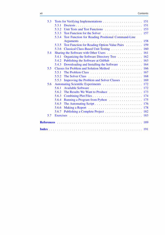
1.1.3 The Backward Euler Scheme
There are several choices of difference approximations in step 3 of the finite differ-ence method as presented in the previous section. Another alternative is
u0.tn/ � un � un�1
tn � tn�1
: (1.8)
Since this difference is based on going backward in time (tn�1) for information, it isknown as a backward difference, also called Backward Euler difference. Figure 1.4explains the idea.
Fig. 1.4 Illustration of a backward difference

8 1 Algorithms and Implementations
Inserting (1.8) in (1.4) yields the Backward Euler (BE) scheme:
un � un�1
tn � tn�1
D �aun; n D 1; : : : ; Nt : (1.9)
We assume, as explained under step 4 in Sect. 1.1.2, that we have computedu0; u1; : : : ; un�1 such that (1.9) can be used to compute un. Note that (1.9) needs n
to start at 1 (then it involves u0, but no u�1) and end at Nt .For direct similarity with the formula for the Forward Euler scheme (1.7) we
replace n by nC 1 in (1.9) and solve for the unknown value unC1:
unC1 D 1
1C a.tnC1 � tn/un; n D 0; : : : ; Nt � 1 : (1.10)
1.1.4 The Crank–Nicolson Scheme
The finite difference approximations (1.5) and (1.8) used to derive the schemes (1.7)and (1.10), respectively, are both one-sided differences, i.e., we collect informationeither forward or backward in time when approximating the derivative at a point.Such one-sided differences are known to be less accurate than central (or midpoint)differences, where we use information both forward and backward in time. A nat-ural next step is therefore to construct a central difference approximation that willyield a more accurate numerical solution.
The central difference approximation to the derivative is sought at the pointtnC 1
2D 1
2.tn C tnC1/ (or tnC 1
2D .n C 1
2/�t if the mesh spacing is uniform in
time). The approximation reads
u0.tnC 12/ � unC1 � un
tnC1 � tn: (1.11)
Figure 1.5 sketches the geometric interpretation of such a centered difference. Notethat the fraction on the right-hand side is the same as for the Forward Euler ap-proximation (1.5) and the Backward Euler approximation (1.8) (with n replaced byn C 1). The accuracy of this fraction as an approximation to the derivative of u
depends on where we seek the derivative: in the center of the interval Œtn; tnC1� or atthe end points. We shall later see that it is more accurate at the center point.
With the formula (1.11), where u0 is evaluated at tnC 12, it is natural to demand
the ODE to be fulfilled at the time points between the mesh points:
u0.tnC 12/ D �au.tnC 1
2/; n D 0; : : : ; Nt � 1 : (1.12)
Using (1.11) in (1.12) results in the approximate discrete equation
unC1 � un
tnC1 � tnD �aunC 1
2 ; n D 0; : : : ; Nt � 1; (1.13)
where unC 12 is a short form for the numerical approximation to u.tnC 1
2/.
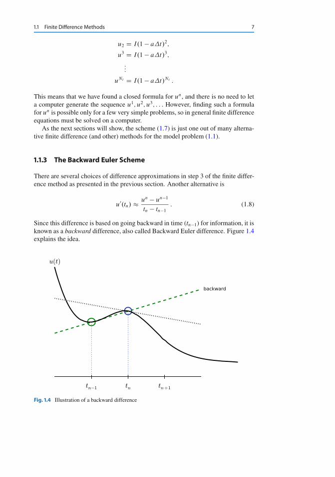
1.1 Finite Difference Methods 9
Fig. 1.5 Illustration of a centered difference
There is a fundamental problem with the right-hand side of (1.13): we aim tocompute un for integer n, which means that unC 1
2 is not a quantity computed byour method. The quantity must therefore be expressed by the quantities that weactually produce, i.e., the numerical solution at the mesh points. One possibility isto approximate unC 1
2 as an arithmetic mean of the u values at the neighboring meshpoints:
unC 12 � 1
2.un C unC1/ : (1.14)
Using (1.14) in (1.13) results in a new approximate discrete equation
unC1 � un
tnC1 � tnD �a
1
2.un C unC1/ : (1.15)
There are three approximation steps leading to this formula: 1) the ODE is onlyvalid at discrete points (between the mesh points), 2) the derivative is approximatedby a finite difference, and 3) the value of u between mesh points is approximatedby an arithmetic mean value. Despite one more approximation than for the Back-ward and Forward Euler schemes, the use of a centered difference leads to a moreaccurate method.
To formulate a recursive algorithm, we assume that un is already computed sothat unC1 is the unknown, which we can solve for:
unC1 D 1 � 12a.tnC1 � tn/
1C 12a.tnC1 � tn/
un : (1.16)
The finite difference scheme (1.16) is often called the Crank–Nicolson (CN) schemeor a midpoint or centered scheme. Note that (1.16) as well as (1.7) and (1.10) applywhether the spacing in the time mesh, tnC1 � tn, depends on n or is constant.

10 1 Algorithms and Implementations
1.1.5 The Unifying �-Rule
The Forward Euler, Backward Euler, and Crank–Nicolson schemes can be formu-lated as one scheme with a varying parameter � :
unC1 � un
tnC1 � tnD �a.�unC1 C .1 � �/un/ : (1.17)
Observe that
� � D 0 gives the Forward Euler scheme� � D 1 gives the Backward Euler scheme,� � D 1
2gives the Crank–Nicolson scheme.
We shall later, in Chap. 2, learn the pros and cons of the three alternatives. One mayalternatively choose any other value of � in Œ0; 1�, but this is not so common sincethe accuracy and stability of the scheme do not improve compared to the values� D 0; 1; 1
2.
As before, un is considered known and unC1 unknown, so we solve for the latter:
unC1 D 1 � .1 � �/a.tnC1 � tn/
1C �a.tnC1 � tn/: (1.18)
This scheme is known as the �-rule, or alternatively written as the “theta-rule”.
DerivationWe start with replacing u0 by the fraction
unC1 � un
tnC1 � tn;
in the Forward Euler, Backward Euler, and Crank–Nicolson schemes. Then weobserve that the difference between the methods concerns which point this frac-tion approximates the derivative. Or in other words, at which point we sample theODE. So far this has been the end points or the midpoint of Œtn; tnC1�. However,we may choose any point Qt 2 Œtn; tnC1�. The difficulty is that evaluating the right-hand side �au at an arbitrary point faces the same problem as in Sect. 1.1.4: thepoint value must be expressed by the discrete u quantities that we compute bythe scheme, i.e., un and unC1. Following the averaging idea from Sect. 1.1.4, thevalue of u at an arbitrary point Qt can be calculated as a weighted average, whichgeneralizes the arithmetic mean 1
2un C 1
2unC1. The weighted average reads
u.Qt / � �unC1 C .1 � �/un; (1.19)
where � 2 Œ0; 1� is a weighting factor. We can also express Qt as a similarweighted average
Qt � � tnC1 C .1 � �/tn : (1.20)
Let now the ODE hold at the point Qt 2 Œtn; tnC1�, approximate u0 by thefraction .unC1 � un/=.tnC1 � tn/, and approximate the right-hand side �au bythe weighted average (1.19). The result is (1.17).

1.1 Finite Difference Methods 11
1.1.6 Constant Time Step
All schemes up to now have been formulated for a general non-uniform mesh intime: t0 < t1 < � � � < tNt
. Non-uniform meshes are highly relevant since onecan use many points in regions where u varies rapidly, and fewer points in regionswhere u is slowly varying. This idea saves the total number of points and thereforemakes it faster to compute the mesh function un. Non-uniform meshes are usedtogether with adaptive methods that are able to adjust the time mesh during thecomputations (Sect. 3.2.11 applies adaptive methods).
However, a uniformly distributed set of mesh points is not only convenient, butalso sufficient for many applications. Therefore, it is a very common choice. Weshall present the finite difference schemes for a uniform point distribution tn Dn�t , where �t is the constant spacing between the mesh points, also referred to asthe time step. The resulting formulas look simpler and are more well known.
Summary of schemes for constant time step
unC1 D .1 � a�t/un Forward Euler (1.21)
unC1 D 1
1C a�tun Backward Euler (1.22)
unC1 D 1 � 12a�t
1C 12a�t
un Crank–Nicolson (1.23)
unC1 D 1 � .1 � �/a�t
1C �a�tun The �-rule (1.24)
It is not accidental that we focus on presenting the Forward Euler, BackwardEuler, and Crank–Nicolson schemes. They complement each other with their dif-ferent pros and cons, thus providing a useful collection of solution methods formany differential equation problems. The unifying notation of the �-rule makes itconvenient to work with all three methods through just one formula. This is par-ticularly advantageous in computer implementations since one avoids if-else testswith formulas that have repetitive elements.
Test your understanding!To check that key concepts are really understood, the reader is encouraged toapply the explained finite difference techniques to a slightly different equation.For this purpose, we recommend you do Exercise 4.2 now!
1.1.7 Mathematical Derivation of Finite Difference Formulas
The finite difference formulas for approximating the first derivative of a functionhave so far been somewhat justified through graphical illustrations in Figs. 1.3,1.4, and 1.5. The task is to approximate the derivative at a point of a curve usingonly two function values. By drawing a straight line through the points, we havesome approximation to the tangent of the curve and use the slope of this line as

12 1 Algorithms and Implementations
an approximation to the derivative. The slope can be computed by inspecting thefigures.
However, we can alternatively derive the finite difference formulas by pure math-ematics. The key tool for this approach is Taylor series, or more precisely, approxi-mation of functions by lower-order Taylor polynomials. Given a function f .x/ thatis sufficiently smooth (i.e., f .x/ has “enough derivatives”), a Taylor polynomial ofdegree m can be used to approximate the value of the function f .x/ if we know thevalues of f and its first m derivatives at some other point x D a. The formula forthe Taylor polynomial reads
f .x/ � f .a/C f 0.a/.x � a/C 1
2f 00.a/.x � a/2 C 1
6f 000.a/.x � a/3 C � � �
C 1
mŠ
df .m/
dxm.a/.x � a/m : (1.25)
For a function of time, f .t/, related to a mesh with spacing �t , we often needthe Taylor polynomial approximation at f .tn ˙ �t/ given f and its derivatives att D tn. Replacing x by tn C�t and a by tn gives
f .tn C�t/ � f .tn/C f 0.tn/�t C 1
2f 00.tn/�t2 C 1
6f 000.tn/�t3 C � � �
C 1
mŠ
df .m/
dxm.tn/�tm : (1.26)
The forward difference We can use (1.26) to find an approximation for f 0.tn/
simply by solving with respect to this quantity:
f 0.tn/ � f .tn C�t/ � f .tn/
�t� 1
2f 00.tn/�t � 1
6f 000.tn/�t2 C � � �
� 1
mŠ
df .m/
dxm.tn/�tm�1 : (1.27)
By letting m!1, this formula is exact, but that is not so much of practical value.A more interesting observation is that all the power terms in �t vanish as �t ! 0,i.e., the formula
f 0.tn/ � f .tn C�t/ � f .tn/
�t(1.28)
is exact in the limit �t ! 0.The interesting feature of (1.27) is that we have a measure of the error in the
formula (1.28): the error is given by the extra terms on the right-hand side of (1.27).We assume that �t is a small quantity (�t � 1). Then �t2 � �t , �t3 � �t2,and so on, which means that the first term is the dominating term. This first termreads � 1
2f 00.tn/�t and can be taken as a measure of the error in the Forward Euler
formula.
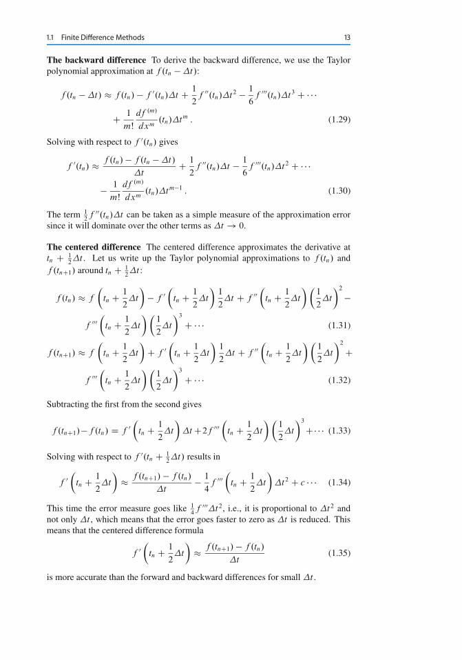
1.1 Finite Difference Methods 13
The backward difference To derive the backward difference, we use the Taylorpolynomial approximation at f .tn ��t/:
f .tn ��t/ � f .tn/ � f 0.tn/�t C 1
2f 00.tn/�t2 � 1
6f 000.tn/�t3 C � � �
C 1
mŠ
df .m/
dxm.tn/�tm : (1.29)
Solving with respect to f 0.tn/ gives
f 0.tn/ � f .tn/� f .tn ��t/
�tC 1
2f 00.tn/�t � 1
6f 000.tn/�t2 C � � �
� 1
mŠ
df .m/
dxm.tn/�tm�1 : (1.30)
The term 12f 00.tn/�t can be taken as a simple measure of the approximation error
since it will dominate over the other terms as �t ! 0.
The centered difference The centered difference approximates the derivative attn C 1
2�t . Let us write up the Taylor polynomial approximations to f .tn/ and
f .tnC1/ around tn C 12�t :
f .tn/ � f
�tn C 1
2�t
�� f 0
�tn C 1
2�t
�1
2�t C f 00
�tn C 1
2�t
��1
2�t
�2
�
f 000�
tn C 1
2�t
��1
2�t
�3
C � � � (1.31)
f .tnC1/ � f
�tn C 1
2�t
�C f 0
�tn C 1
2�t
�1
2�t C f 00
�tn C 1
2�t
��1
2�t
�2
C
f 000�
tn C 1
2�t
��1
2�t
�3
C � � � (1.32)
Subtracting the first from the second gives
f .tnC1/�f .tn/ D f 0�
tn C 1
2�t
��tC2f 000
�tn C 1
2�t
��1
2�t
�3
C� � � (1.33)
Solving with respect to f 0.tn C 12�t/ results in
f 0�
tn C 1
2�t
�� f .tnC1/ � f .tn/
�t� 1
4f 000
�tn C 1
2�t
��t2 C c � � � (1.34)
This time the error measure goes like 14f 000�t2, i.e., it is proportional to �t2 and
not only �t , which means that the error goes faster to zero as �t is reduced. Thismeans that the centered difference formula
f 0�
tn C 1
2�t
�� f .tnC1/� f .tn/
�t(1.35)
is more accurate than the forward and backward differences for small �t .
14 1 Algorithms and Implementations
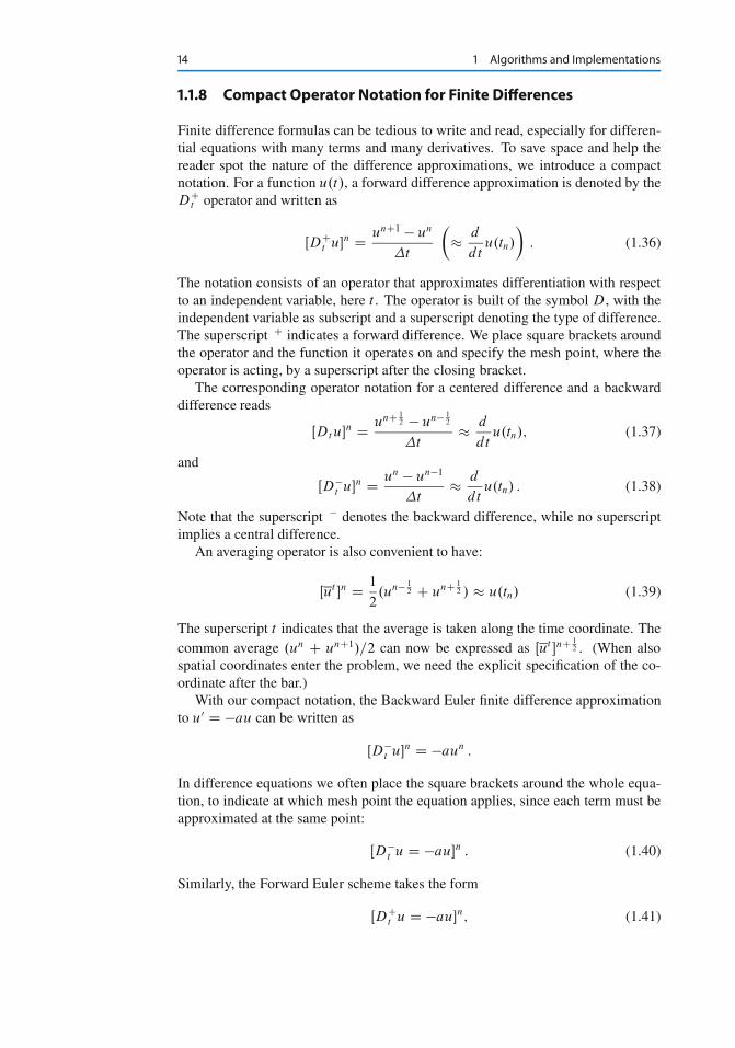
1.1.8 Compact Operator Notation for Finite Differences
Finite difference formulas can be tedious to write and read, especially for differen-tial equations with many terms and many derivatives. To save space and help thereader spot the nature of the difference approximations, we introduce a compactnotation. For a function u.t/, a forward difference approximation is denoted by theDCt operator and written as
ŒDCt u�n D unC1 � un
�t
�� d
dtu.tn/
�: (1.36)
The notation consists of an operator that approximates differentiation with respectto an independent variable, here t . The operator is built of the symbol D, with theindependent variable as subscript and a superscript denoting the type of difference.The superscript C indicates a forward difference. We place square brackets aroundthe operator and the function it operates on and specify the mesh point, where theoperator is acting, by a superscript after the closing bracket.
The corresponding operator notation for a centered difference and a backwarddifference reads
ŒDt u�n D unC 12 � un� 1
2
�t� d
dtu.tn/; (1.37)
and
ŒD�t u�n D un � un�1
�t� d
dtu.tn/ : (1.38)
Note that the superscript � denotes the backward difference, while no superscriptimplies a central difference.
An averaging operator is also convenient to have:
Œut �n D 1
2.un� 1
2 C unC 12 / � u.tn/ (1.39)
The superscript t indicates that the average is taken along the time coordinate. Thecommon average .un C unC1/=2 can now be expressed as Œut �nC
12 . (When also
spatial coordinates enter the problem, we need the explicit specification of the co-ordinate after the bar.)
With our compact notation, the Backward Euler finite difference approximationto u0 D �au can be written as
ŒD�t u�n D �aun :
In difference equations we often place the square brackets around the whole equa-tion, to indicate at which mesh point the equation applies, since each term must beapproximated at the same point:
ŒD�t u D �au�n : (1.40)
Similarly, the Forward Euler scheme takes the form
ŒDCt u D �au�n; (1.41)

1.2 Implementations 15
while the Crank–Nicolson scheme is written as
ŒDt u D �aut �nC12 : (1.42)
QuestionBy use of (1.37) and (1.39), are you able to write out the expressions in (1.42) toverify that it is indeed the Crank–Nicolson scheme?
The �-rule can be specified in operator notation by
Œ NDt u D �aut;� �nC� : (1.43)
We define a new time difference
Œ NDt u�nC� D unC1 � un
tnC1 � tn; (1.44)
to be applied at the time point tnC� � � tn C .1 � �/tnC1. This weighted averagegives rise to the weighted averaging operator
Œut;� �nC� D .1 � �/un C �unC1 � u.tnC� /; (1.45)
where � 2 Œ0; 1� as usual. Note that for � D 12
we recover the standard cen-tered difference and the standard arithmetic mean. The idea in (1.43) is to samplethe equation at tnC� , use a non-symmetric difference at that point Œ NDtu�nC� , anda weighted (non-symmetric) mean value.
An alternative and perhaps clearer notation is
ŒDtu�nC12 D �Œ�au�nC1C .1 � �/Œ�au�n :
Looking at the various examples above and comparing them with the underlyingdifferential equations, we see immediately which difference approximations thathave been used and at which point they apply. Therefore, the compact notationeffectively communicates the reasoning behind turning a differential equation intoa difference equation.
1.2 Implementations
We want to make a computer program for solving
u0.t/ D �au.t/; t 2 .0; T �; u.0/ D I;
by finite difference methods. The program should also display the numerical solu-tion as a curve on the screen, preferably together with the exact solution.
All programs referred to in this section are found in the src/alg1 directory (weuse the classical Unix term directory for what many others nowadays call folder).
1 http://tinyurl.com/ofkw6kc/alg
16 1 Algorithms and Implementations
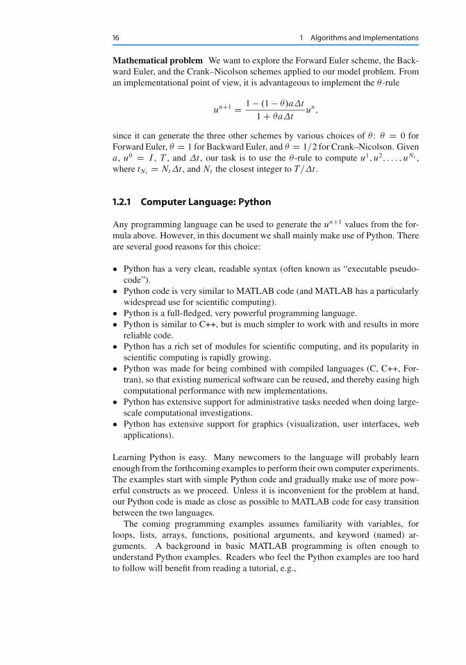
Mathematical problem We want to explore the Forward Euler scheme, the Back-ward Euler, and the Crank–Nicolson schemes applied to our model problem. Froman implementational point of view, it is advantageous to implement the �-rule
unC1 D 1 � .1 � �/a�t
1C �a�tun;
since it can generate the three other schemes by various choices of � : � D 0 forForward Euler, � D 1 for Backward Euler, and � D 1=2 for Crank–Nicolson. Givena, u0 D I , T , and �t , our task is to use the �-rule to compute u1; u2; : : : ; uNt ,where tNt
D Nt �t , and Nt the closest integer to T=�t .
1.2.1 Computer Language: Python
Any programming language can be used to generate the unC1 values from the for-mula above. However, in this document we shall mainly make use of Python. Thereare several good reasons for this choice:
� Python has a very clean, readable syntax (often known as “executable pseudo-code”).
� Python code is very similar to MATLAB code (and MATLAB has a particularlywidespread use for scientific computing).
� Python is a full-fledged, very powerful programming language.� Python is similar to C++, but is much simpler to work with and results in more
reliable code.� Python has a rich set of modules for scientific computing, and its popularity in
scientific computing is rapidly growing.� Python was made for being combined with compiled languages (C, C++, For-
tran), so that existing numerical software can be reused, and thereby easing highcomputational performance with new implementations.
� Python has extensive support for administrative tasks needed when doing large-scale computational investigations.
� Python has extensive support for graphics (visualization, user interfaces, webapplications).
Learning Python is easy. Many newcomers to the language will probably learnenough from the forthcoming examples to perform their own computer experiments.The examples start with simple Python code and gradually make use of more pow-erful constructs as we proceed. Unless it is inconvenient for the problem at hand,our Python code is made as close as possible to MATLAB code for easy transitionbetween the two languages.
The coming programming examples assumes familiarity with variables, forloops, lists, arrays, functions, positional arguments, and keyword (named) ar-guments. A background in basic MATLAB programming is often enough tounderstand Python examples. Readers who feel the Python examples are too hardto follow will benefit from reading a tutorial, e.g.,

1.2 Implementations 17
� The Official Python Tutorial2
� Python Tutorial on tutorialspoint.com3
� Interactive Python tutorial site4
� A Beginner’s Python Tutorial5
The author also has a comprehensive book [8] that teaches scientific programmingwith Python from the ground up.
1.2.2 Making a Solver Function
We choose to have an array u for storing the un values, n D 0; 1; : : : ; Nt . Thealgorithmic steps are
1. initialize u0
2. for t D tn, n D 1; 2; : : : ; Nt : compute un using the �-rule formula
An implementation of a numerical algorithm is often referred to as a solver. Weshall now make a solver for our model problem and realize the solver as a Pythonfunction. The function must take the input data I , a, T , �t , and � of the problemas arguments and return the solution as arrays u and t for un and tn, n D 0; : : : ; Nt .The solver function used as
u, t = solver(I, a, T, dt, theta)
One can now easily plot u versus t to visualize the solution.The function solver may look as follows in Python:
from numpy import *
def solver(I, a, T, dt, theta):"""Solve u’=-a*u, u(0)=I, for t in (0,T] with steps of dt."""Nt = int(T/dt) # no of time intervalsT = Nt*dt # adjust T to fit time step dtu = zeros(Nt+1) # array of u[n] valuest = linspace(0, T, Nt+1) # time mesh
u[0] = I # assign initial conditionfor n in range(0, Nt): # n=0,1,...,Nt-1
u[n+1] = (1 - (1-theta)*a*dt)/(1 + theta*dt*a)*u[n]return u, t
The numpy library contains a lot of functions for array computing. Most of thefunction names are similar to what is found in the alternative scientific computinglanguage MATLAB. Here we make use of
� zeros(Nt+1) for creating an array of size Nt+1 and initializing the elements tozero
2 http://docs.python.org/2/tutorial/3 http://www.tutorialspoint.com/python/4 http://www.learnpython.org/5 http://en.wikibooks.org/wiki/A_Beginner’s_Python_Tutorial

18 1 Algorithms and Implementations
� linspace(0, T, Nt+1) for creating an array with Nt+1 coordinates uniformlydistributed between 0 and T
The for loop deserves a comment, especially for newcomers to Python. The con-struction range(0, Nt, s) generates all integers from 0 to Nt in steps of s, butnot including Nt. Omitting s means s=1. For example, range(0, 6, 3) gives 0and 3, while range(0, 6) generates the list [0, 1, 2, 3, 4, 5]. Our loop im-plies the following assignments to u[n+1]: u[1], u[2], . . . , u[Nt], which is whatwe want since u has length Nt+1. The first index in Python arrays or lists is always0 and the last is then len(u)-1 (the length of an array u is obtained by len(u) oru.size).
1.2.3 Integer Division
The shown implementation of the solver may face problems and wrong results ifT, a, dt, and theta are given as integers (see Exercises 1.3 and 1.4). The prob-lem is related to integer division in Python (as in Fortran, C, C++, and many othercomputer languages!): 1/2 becomes 0, while 1.0/2, 1/2.0, or 1.0/2.0 all be-come 0.5. So, it is enough that at least the nominator or the denominator is a realnumber (i.e., a float object) to ensure a correct mathematical division. Insertinga conversion dt = float(dt) guarantees that dt is float.
Another problem with computing Nt D T=�t is that we should round Nt tothe nearest integer. With Nt = int(T/dt) the int operation picks the largestinteger smaller than T/dt. Correct mathematical rounding as known from school isobtained by
Nt = int(round(T/dt))
The complete version of our improved, safer solver function then becomes
from numpy import *
def solver(I, a, T, dt, theta):"""Solve u’=-a*u, u(0)=I, for t in (0,T] with steps of dt."""dt = float(dt) # avoid integer divisionNt = int(round(T/dt)) # no of time intervalsT = Nt*dt # adjust T to fit time step dtu = zeros(Nt+1) # array of u[n] valuest = linspace(0, T, Nt+1) # time mesh
u[0] = I # assign initial conditionfor n in range(0, Nt): # n=0,1,...,Nt-1
u[n+1] = (1 - (1-theta)*a*dt)/(1 + theta*dt*a)*u[n]return u, t
1.2.4 Doc Strings
Right below the header line in the solver function there is a Python string enclosedin triple double quotes """. The purpose of this string object is to document whatthe function does and what the arguments are. In this case the necessary documen-

1.2 Implementations 19
tation does not span more than one line, but with triple double quoted strings thetext may span several lines:
def solver(I, a, T, dt, theta):"""Solve
u’(t) = -a*u(t),
with initial condition u(0)=I, for t in the time interval(0,T]. The time interval is divided into time steps oflength dt.
theta=1 corresponds to the Backward Euler scheme, theta=0to the Forward Euler scheme, and theta=0.5 to the Crank-Nicolson method."""...
Such documentation strings appearing right after the header of a function are calleddoc strings. There are tools that can automatically produce nicely formatted docu-mentation by extracting the definition of functions and the contents of doc strings.
It is strongly recommended to equip any function with a doc string, unless thepurpose of the function is not obvious. Nevertheless, the forthcoming text deviatesfrom this rule if the function is explained in the text.
1.2.5 Formatting Numbers
Having computed the discrete solution u, it is natural to look at the numbers:
# Write out a table of t and u values:for i in range(len(t)):
print t[i], u[i]
This compact print statement unfortunately gives less readable output because thet and u values are not aligned in nicely formatted columns. To fix this problem,we recommend to use the printf format, supported in most programming languagesinherited from C. Another choice is Python’s recent format string syntax. Bothkinds of syntax are illustrated below.
Writing t[i] and u[i] in two nicely formatted columns is done like this withthe printf format:
print ’t=%6.3f u=%g’ % (t[i], u[i])
The percentage signs signify “slots” in the text where the variables listed at the endof the statement are inserted. For each “slot” one must specify a format for how thevariable is going to appear in the string: f for float (with 6 decimals), s for puretext, d for an integer, g for a real number written as compactly as possible, 9.3Efor scientific notation with three decimals in a field of width 9 characters (e.g.,-1.351E-2), or .2f for standard decimal notation with two decimals formatted

20 1 Algorithms and Implementations
with minimum width. The printf syntax provides a quick way of formatting tabularoutput of numbers with full control of the layout.
The alternative format string syntax looks like
print ’t={t:6.3f} u={u:g}’.format(t=t[i], u=u[i])
As seen, this format allows logical names in the “slots” where t[i] and u[i] areto be inserted. The “slots” are surrounded by curly braces, and the logical nameis followed by a colon and then the printf-like specification of how to format realnumbers, integers, or strings.
1.2.6 Running the Program
The function and main program shown above must be placed in a file, say withname decay_v1.py6 (v1 for 1st version of this program). Make sure you write thecode with a suitable text editor (Gedit, Emacs, Vim, Notepad++, or similar). Theprogram is run by executing the file this way:
Terminal
Terminal> python decay_v1.py
The text Terminal> just indicates a prompt in a Unix/Linux or DOS termi-nal window. After this prompt, which may look different in your terminal win-dow (depending on the terminal application and how it is set up), commands likepython decay_v1.py can be issued. These commands are interpreted by the op-erating system.
We strongly recommend to run Python programs within the IPython shell. Firststart IPython by typing ipython in the terminal window. Inside the IPython shell,our program decay_v1.py is run by the command run decay_v1.py:
Terminal
Terminal> ipython
In [1]: run decay_v1.pyt= 0.000 u=1t= 0.800 u=0.384615t= 1.600 u=0.147929t= 2.400 u=0.0568958t= 3.200 u=0.021883t= 4.000 u=0.00841653t= 4.800 u=0.00323713t= 5.600 u=0.00124505t= 6.400 u=0.000478865t= 7.200 u=0.000184179t= 8.000 u=7.0838e-05
6 http://tinyurl.com/ofkw6kc/alg/decay_v1.py

1.2 Implementations 21
The advantage of running programs in IPython are many, but here we explicitlymention a few of the most useful features:
� previous commands are easily recalled with the up arrow,� %pdb turns on a debugger so that variables can be examined if the program aborts
(due to a Python exception),� output of commands are stored in variables,� the computing time spent on a set of statements can be measured with the
%timeit command,� any operating system command can be executed,� modules can be loaded automatically and other customizations can be performed
when starting IPython
Although running programs in IPython is strongly recommended, most executionexamples in the forthcoming text use the standard Python shell with prompt »> andrun programs through a typesetting like
Terminal
Terminal> python programname
The reason is that such typesetting makes the text more compact in the verticaldirection than showing sessions with IPython syntax.
1.2.7 Plotting the Solution
Having the t and u arrays, the approximate solution u is visualized by the intuitivecommand plot(t, u):
from matplotlib.pyplot import *plot(t, u)show()
It will be illustrative to also plot the exact solution ue.t/ D Ie�at for comparison.We first need to make a Python function for computing the exact solution:
def u_exact(t, I, a):return I*exp(-a*t)
It is tempting to just do
u_e = u_exact(t, I, a)plot(t, u, t, u_e)
However, this is not exactly what we want: the plot function draws straight linesbetween the discrete points (t[n], u_e[n]) while ue.t/ varies as an exponential

22 1 Algorithms and Implementations
function between the mesh points. The technique for showing the “exact” variationof ue.t/ between the mesh points is to introduce a very fine mesh for ue.t/:
t_e = linspace(0, T, 1001) # fine meshu_e = u_exact(t_e, I, a)
We can also plot the curves with different colors and styles, e.g.,
plot(t_e, u_e, ’b-’, # blue line for u_et, u, ’r--o’) # red dashes w/circles
With more than one curve in the plot we need to associate each curve witha legend. We also want appropriate names on the axes, a title, and a file con-taining the plot as an image for inclusion in reports. The Matplotlib package(matplotlib.pyplot) contains functions for this purpose. The names of thefunctions are similar to the plotting functions known from MATLAB. A completefunction for creating the comparison plot becomes
from matplotlib.pyplot import *
def plot_numerical_and_exact(theta, I, a, T, dt):"""Compare the numerical and exact solution in a plot."""u, t = solver(I=I, a=a, T=T, dt=dt, theta=theta)
t_e = linspace(0, T, 1001) # fine mesh for u_eu_e = u_exact(t_e, I, a)
plot(t, u, ’r--o’, # red dashes w/circlest_e, u_e, ’b-’) # blue line for exact sol.
legend([’numerical’, ’exact’])xlabel(’t’)ylabel(’u’)title(’theta=%g, dt=%g’ % (theta, dt))savefig(’plot_%s_%g.png’ % (theta, dt))
plot_numerical_and_exact(I=1, a=2, T=8, dt=0.8, theta=1)show()
Note that savefig here creates a PNG file whose name includes the values of �
and �t so that we can easily distinguish files from different runs with � and �t .The complete code is found in the file decay_v2.py7. The resulting plot is
shown in Fig. 1.6. As seen, there is quite some discrepancy between the exact andthe numerical solution. Fortunately, the numerical solution approaches the exactone as �t is reduced.
1.2.8 Verifying the Implementation
It is easy to make mistakes while deriving and implementing numerical algorithms,so we should never believe in the solution before it has been thoroughly verified.
7 http://tinyurl.com/ofkw6kc/alg/decay_v2.py

1.2 Implementations 23
Fig. 1.6 Comparison of numerical and exact solution
Verification and validationThe purpose of verifying a program is to bring evidence for the property that thereare no errors in the implementation. A related term, validate (and validation),addresses the question if the ODE model is a good representation of the phenom-ena we want to simulate. To remember the difference between verification andvalidation, verification is about solving the equations right, while validation isabout solving the right equations. We must always perform a verification beforeit is meaningful to believe in the computations and perform validation (whichcompares the program results with physical experiments or observations).
The most obvious idea for verification in our case is to compare the numerical so-lution with the exact solution, when that exists. This is, however, not a particularlygood method. The reason is that there will always be a discrepancy between thesetwo solutions, due to numerical approximations, and we cannot precisely quantifythe approximation errors. The open question is therefore whether we have the math-ematically correct discrepancy or if we have another, maybe small, discrepancy dueto both an approximation error and an error in the implementation. It is thus impos-sible to judge whether the program is correct or not by just looking at the graphs inFig. 1.6.
To avoid mixing the unavoidable numerical approximation errors and the unde-sired implementation errors, we should try to make tests where we have some exactcomputation of the discrete solution or at least parts of it. Examples will show howthis can be done.
Running a few algorithmic steps by hand The simplest approach to producea correct non-trivial reference solution for the discrete solution u, is to computea few steps of the algorithm by hand. Then we can compare the hand calculationswith numbers produced by the program.
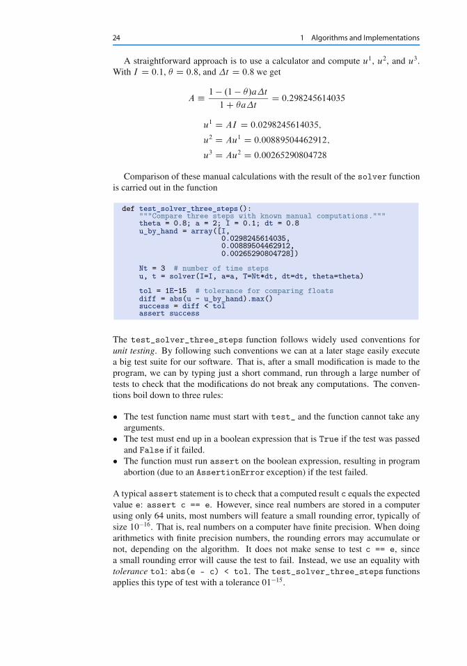
24 1 Algorithms and Implementations
A straightforward approach is to use a calculator and compute u1, u2, and u3.With I D 0:1, � D 0:8, and �t D 0:8 we get
A � 1 � .1 � �/a�t
1C �a�tD 0:298245614035
u1 D AI D 0:0298245614035;
u2 D Au1 D 0:00889504462912;
u3 D Au2 D 0:00265290804728
Comparison of these manual calculations with the result of the solver functionis carried out in the function
def test_solver_three_steps():"""Compare three steps with known manual computations."""theta = 0.8; a = 2; I = 0.1; dt = 0.8u_by_hand = array([I,
0.0298245614035,0.00889504462912,0.00265290804728])
Nt = 3 # number of time stepsu, t = solver(I=I, a=a, T=Nt*dt, dt=dt, theta=theta)
tol = 1E-15 # tolerance for comparing floatsdiff = abs(u - u_by_hand).max()success = diff < tolassert success
The test_solver_three_steps function follows widely used conventions forunit testing. By following such conventions we can at a later stage easily executea big test suite for our software. That is, after a small modification is made to theprogram, we can by typing just a short command, run through a large number oftests to check that the modifications do not break any computations. The conven-tions boil down to three rules:
� The test function name must start with test_ and the function cannot take anyarguments.
� The test must end up in a boolean expression that is True if the test was passedand False if it failed.
� The function must run assert on the boolean expression, resulting in programabortion (due to an AssertionError exception) if the test failed.
A typical assert statement is to check that a computed result c equals the expectedvalue e: assert c == e. However, since real numbers are stored in a computerusing only 64 units, most numbers will feature a small rounding error, typically ofsize 10�16. That is, real numbers on a computer have finite precision. When doingarithmetics with finite precision numbers, the rounding errors may accumulate ornot, depending on the algorithm. It does not make sense to test c == e, sincea small rounding error will cause the test to fail. Instead, we use an equality withtolerance tol: abs(e - c) < tol. The test_solver_three_steps functionsapplies this type of test with a tolerance 01�15.

1.2 Implementations 25
The main program can routinely run the verification test prior to solving the realproblem:
test_solver_three_steps()plot_numerical_and_exact(I=1, a=2, T=8, dt=0.8, theta=1)show()
(Rather than calling test_*() functions explicitly, one will normally ask a test-ing framework like nose or pytest to find and run such functions.) The completeprogram including the verification above is found in the file decay_v3.py8.
1.2.9 Computing the Numerical Error as a Mesh Function
Now that we have some evidence for a correct implementation, we are in position tocompare the computed un values in the u array with the exact u values at the meshpoints, in order to study the error in the numerical solution.
A natural way to compare the exact and discrete solutions is to calculate theirdifference as a mesh function for the error:
en D ue.tn/ � un; n D 0; 1; : : : ; Nt : (1.46)
We may view the mesh function une D ue.tn/ as a representation of the continuous
function ue.t/ defined for all t 2 Œ0; T �. In fact, une is often called the representative
of ue on the mesh. Then, en D une � un is clearly the difference of two mesh
functions.The error mesh function en can be computed by
u, t = solver(I, a, T, dt, theta) # Numerical sol.u_e = u_exact(t, I, a) # Representative of exact sol.e = u_e - u
Note that the mesh functions u and u_e are represented by arrays and associatedwith the points in the array t.
Array arithmeticsThe last statements
u_e = u_exact(t, I, a)e = u_e - u
demonstrate some standard examples of array arithmetics: t is an array of meshpoints that we pass to u_exact. This function evaluates -a*t, which is a scalartimes an array, meaning that the scalar is multiplied with each array element.The result is an array, let us call it tmp1. Then exp(tmp1) means applyingthe exponential function to each element in tmp1, giving an array, say tmp2.
8 http://tinyurl.com/ofkw6kc/alg/decay_v3.py

26 1 Algorithms and Implementations
Finally, I*tmp2 is computed (scalar times array) and u_e refers to this arrayreturned from u_exact. The expression u_e - u is the difference between twoarrays, resulting in a new array referred to by e.
Replacement of array element computations inside a loop by array arithmeticsis known as vectorization.
1.2.10 Computing the Norm of the Error Mesh Function
Instead of working with the error en on the entire mesh, we often want a singlenumber expressing the size of the error. This is obtained by taking the norm of theerror function.
Let us first define norms of a function f .t/ defined for all t 2 Œ0; T �. Threecommon norms are
jjf jjL2 D0@
TZ0
f .t/2dt
1A
1=2
; (1.47)
jjf jjL1 DTZ
0
jf .t/jdt; (1.48)
jjf jjL1 D maxt2Œ0;T �
jf .t/j : (1.49)
The L2 norm (1.47) (“L-two norm”) has nice mathematical properties and is themost popular norm. It is a generalization of the well-known Eucledian norm ofvectors to functions. The L1 norm looks simpler and more intuitive, but has lessnice mathematical properties compared to the two other norms, so it is much lessused in computations. The L1 is also called the max norm or the supremum normand is widely used. It focuses on a single point with the largest value of jf j, whilethe other norms measure average behavior of the function.
In fact, there is a whole family of norms,
jjf jjLp D0@
TZ0
f .t/pdt
1A
1=p
; (1.50)
with p real. In particular, p D 1 corresponds to the L1 norm above while p D 1is the L1 norm.
Numerical computations involving mesh functions need corresponding norms.Given a set of function values, f n, and some associated mesh points, tn, a numer-ical integration rule can be used to calculate the L2 and L1 norms defined above.Imagining that the mesh function is extended to vary linearly between the meshpoints, the Trapezoidal rule is in fact an exact integration rule. A possible modifi-cation of the L2 norm for a mesh function f n on a uniform mesh with spacing �t

1.2 Implementations 27
is therefore the well-known Trapezoidal integration formula
jjf njj D
�t
1
2.f 0/2 C 1
2.f Nt /2 C
Nt�1XnD1
.f n/2
!!1=2
A common approximation of this expression, motivated by the convenience of hav-ing a simpler formula, is
jjf njj`2 D
�t
NtXnD0
.f n/2
!1=2
:
This is called the discrete L2 norm and denoted by `2. If jjf jj2`2 (i.e., the square
of the norm) is used instead of the Trapezoidal integration formula, the error is�t..f 0/2 C .f Nt /2/=2. This means that the weights at the end points of the meshfunction are perturbed, but as �t ! 0, the error from this perturbation goes to zero.As long as we are consistent and stick to one kind of integration rule for the normof a mesh function, the details and accuracy of this rule is of no concern.
The three discrete norms for a mesh function f n, corresponding to the L2, L1,and L1 norms of f .t/ defined above, are defined by
jjf njj`2 D
�t
NtXnD0
.f n/2
!1=2
; (1.51)
jjf njj`1 D �t
NtXnD0
jf nj; (1.52)
jjf njj`1 D max0�n�Nt
jf nj : (1.53)
Note that the L2, L1, `2, and `1 norms depend on the length of the interval ofinterest (think of f D 1, then the norms are proportional to
pT or T ). In some
applications it is convenient to think of a mesh function as just a vector of functionvalues without any relation to the interval Œ0; T �. Then one can replace �t by T=Nt
and simply drop T (which is just a common scaling factor in the norm, independentof the vector of function values). Moreover, people prefer to divide by the totallength of the vector, Nt C 1, instead of Nt . This reasoning gives rise to the vectornorms for a vector f D .f0; : : : ; fN /:
jjf jj2 D
1
N C 1
NXnD0
.fn/2
!1=2
; (1.54)
jjf jj1 D 1
N C 1
NXnD0
jfnj; (1.55)
jjf jj`1 D max0�n�N
jfnj : (1.56)

28 1 Algorithms and Implementations
Here we have used the common vector component notation with subscripts (fn)and N as length. We will mostly work with mesh functions and use the discrete`2 norm (1.51) or the max norm `1 (1.53), but the corresponding vector norms(1.54)–(1.56) are also much used in numerical computations, so it is important toknow the different norms and the relations between them.
A single number that expresses the size of the numerical error will be taken asjjenjj`2 and called E:
E Dvuut�t
NtXnD0
.en/2 (1.57)
The corresponding Python code, using array arithmetics, reads
E = sqrt(dt*sum(e**2))
The sum function comes from numpy and computes the sum of the elements of anarray. Also the sqrt function is from numpy and computes the square root of eachelement in the array argument.
Scalar computing Instead of doing array computing sqrt(dt*sum(e**2)) wecan compute with one element at a time:
m = len(u) # length of u array (alt: u.size)u_e = zeros(m)t = 0for i in range(m):
u_e[i] = u_exact(t, a, I)t = t + dt
e = zeros(m)for i in range(m):
e[i] = u_e[i] - u[i]s = 0 # summation variablefor i in range(m):
s = s + e[i]**2error = sqrt(dt*s)
Such element-wise computing, often called scalar computing, takes more code, isless readable, and runs much slower than what we can achieve with array comput-ing.
1.2.11 Experiments with Computing and Plotting
Let us write down a new function that wraps up the computation and all the plottingstatements used for comparing the exact and numerical solutions. This function canbe called with various � and �t values to see how the error depends on the methodand mesh resolution.
def explore(I, a, T, dt, theta=0.5, makeplot=True):"""Run a case with the solver, compute error measure,and plot the numerical and exact solutions (if makeplot=True)."""

1.2 Implementations 29
u, t = solver(I, a, T, dt, theta) # Numerical solutionu_e = u_exact(t, I, a)e = u_e - uE = sqrt(dt*sum(e**2))if makeplot:
figure() # create new plott_e = linspace(0, T, 1001) # fine mesh for u_eu_e = u_exact(t_e, I, a)plot(t, u, ’r--o’) # red dashes w/circlesplot(t_e, u_e, ’b-’) # blue line for exact sol.legend([’numerical’, ’exact’])xlabel(’t’)ylabel(’u’)title(’theta=%g, dt=%g’ % (theta, dt))theta2name = {0: ’FE’, 1: ’BE’, 0.5: ’CN’}savefig(’%s_%g.png’ % (theta2name[theta], dt))savefig(’%s_%g.pdf’ % (theta2name[theta], dt))show()
return E
The figure() call is key: without it, a new plot command will draw the newpair of curves in the same plot window, while we want the different pairs to appearin separate windows and files. Calling figure() ensures this.
Instead of including the � value in the filename to implicitly inform about theapplied method, the code utilizes a little Python dictionary that maps each relevant� value to a corresponding acronym for the method name (FE, BE, or CN):
theta2name = {0: ’FE’, 1: ’BE’, 0.5: ’CN’}savefig(’%s_%g.png’ % (theta2name[theta], dt))
The explore function stores the plot in two different image file formats: PNGand PDF. The PNG format is suitable for being included in HTML documents,while the PDF format provides higher quality for LATEX (i.e., PDFLATEX) documents.Frequently used viewers for these image files on Unix systems are gv (comes withGhostscript) for the PDF format and display (from the ImageMagick softwaresuite) for PNG files:
Terminal
Terminal> gv BE_0.5.pdfTerminal> display BE_0.5.png
A main program may run a loop over the three methods (given by their corre-sponding � values) and call explore to compute errors and make plots:
def main(I, a, T, dt_values, theta_values=(0, 0.5, 1)):print ’theta dt error’ # Column headings in tablefor theta in theta_values:
for dt in dt_values:E = explore(I, a, T, dt, theta, makeplot=True)print ’%4.1f %6.2f: %12.3E’ % (theta, dt, E)
main(I=1, a=2, T=5, dt_values=[0.4, 0.04])

30 1 Algorithms and Implementations
Fig. 1.7 The Forward Euler scheme for two values of the time step
The file decay_plot_mpl.py9 contains the complete code with the functionsabove. Running this program results in
Terminal
Terminal> python decay_plot_mpl.pytheta dt error0.0 0.40: 2.105E-010.0 0.04: 1.449E-020.5 0.40: 3.362E-020.5 0.04: 1.887E-041.0 0.40: 1.030E-011.0 0.04: 1.382E-02
We observe that reducing �t by a factor of 10 increases the accuracy for allthree methods. We also see that the combination of � D 0:5 and a small time step�t D 0:04 gives a much more accurate solution, and that � D 0 and � D 1 with�t D 0:4 result in the least accurate solutions.
Figure 1.7 demonstrates that the numerical solution produced by the ForwardEuler method with �t D 0:4 clearly lies below the exact curve, but that the accuracyimproves considerably by reducing the time step by a factor of 10.
The behavior of the two other schemes is shown in Figs. 1.8 and 1.9. Crank–Nicolson is obviously the most accurate scheme from this visual point of view.
Combining plot files Mounting two PNG files beside each other, as done inFigs. 1.7–1.9, is easily carried out by the montage10 program from the ImageMag-ick suite:
Terminal
Terminal> montage -background white -geometry 100% -tile 2x1 \FE_0.4.png FE_0.04.png FE1.png
Terminal> convert -trim FE1.png FE1.png
9 http://tinyurl.com/ofkw6kc/alg/decay_plot_mpl.py10 http://www.imagemagick.org/script/montage.php

1.2 Implementations 31
Fig. 1.8 The Backward Euler scheme for two values of the time step
Fig. 1.9 The Crank–Nicolson scheme for two values of the time step
The -geometry argument is used to specify the size of the image. Here, wepreserve the individual sizes of the images. The -tile HxV option specifies H im-ages in the horizontal direction and V images in the vertical direction. A series ofimage files to be combined are then listed, with the name of the resulting com-bined image, here FE1.png at the end. The convert -trim command removessurrounding white areas in the figure (an operation usually known as cropping inimage manipulation programs).
For LATEX reports it is not recommended to use montage and PNG files as theresult has too low resolution. Instead, plots should be made in the PDF format andcombined using the pdftk, pdfnup, and pdfcrop tools (on Linux/Unix):
Terminal
Terminal> pdftk FE_0.4.png FE_0.04.png output tmp.pdfTerminal> pdfnup --nup 2x1 --outfile tmp.pdf tmp.pdfTerminal> pdfcrop tmp.pdf FE1.png # output in FE1.png
Here, pdftk combines images into a multi-page PDF file, pdfnup combinesthe images in individual pages to a table of images (pages), and pdfcrop removeswhite margins in the resulting combined image file.

32 1 Algorithms and Implementations
Plotting with SciTools The SciTools package11 provides a unified plotting inter-face, called Easyviz, to many different plotting packages, including Matplotlib,Gnuplot, Grace, MATLAB, VTK, OpenDX, and VisIt. The syntax is very similar tothat of Matplotlib and MATLAB. In fact, the plotting commands shown above lookthe same in SciTool’s Easyviz interface, apart from the import statement, whichreads
from scitools.std import *
This statement performs a from numpy import * as well as an import of the mostcommon pieces of the Easyviz (scitools.easyviz) package, along with someadditional numerical functionality.
With Easyviz one can merge several plotting commands into a single one usingkeyword arguments:
plot(t, u, ’r--o’, # red dashes w/circlest_e, u_e, ’b-’, # blue line for exact sol.legend=[’numerical’, ’exact’],xlabel=’t’,ylabel=’u’,title=’theta=%g, dt=%g’ % (theta, dt),savefig=’%s_%g.png’ % (theta2name[theta], dt),show=True)
The decay_plot_st.py12 file contains such a demo.By default, Easyviz employs Matplotlib for plotting, but Gnuplot13 and Grace14
are viable alternatives:
Terminal
Terminal> python decay_plot_st.py --SCITOOLS_easyviz_backend gnuplotTerminal> python decay_plot_st.py --SCITOOLS_easyviz_backend grace
The actual tool used for creating plots (called backend) and numerous other op-tions can be permanently set in SciTool’s configuration file.
All the Gnuplot windows are launched without any need to kill one before thenext one pops up (as is the case with Matplotlib) and one can press the key ‘q’anywhere in a plot window to kill it. Another advantage of Gnuplot is the auto-matic choice of sensible and distinguishable line types in black-and-white PDF andPostScript files.
For more detailed information on syntax and plotting capabilities, we refer to theMatplotlib [5] and SciTools [7] documentation. The hope is that the programmingsyntax explained so far suffices for understanding the basic plotting functionalityand being able to look up the cited technical documentation.
11 https://github.com/hplgit/scitools12 http://tinyurl.com/ofkw6kc/alg/decay_plot_st.py13 http://www.gnuplot.info/14 http://plasma-gate.weizmann.ac.il/Grace/
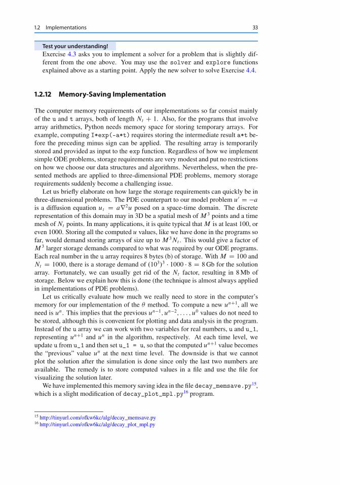
1.2 Implementations 33
Test your understanding!Exercise 4.3 asks you to implement a solver for a problem that is slightly dif-ferent from the one above. You may use the solver and explore functionsexplained above as a starting point. Apply the new solver to solve Exercise 4.4.
1.2.12 Memory-Saving Implementation
The computer memory requirements of our implementations so far consist mainlyof the u and t arrays, both of length Nt C 1. Also, for the programs that involvearray arithmetics, Python needs memory space for storing temporary arrays. Forexample, computing I*exp(-a*t) requires storing the intermediate result a*t be-fore the preceding minus sign can be applied. The resulting array is temporarilystored and provided as input to the exp function. Regardless of how we implementsimple ODE problems, storage requirements are very modest and put no restrictionson how we choose our data structures and algorithms. Nevertheless, when the pre-sented methods are applied to three-dimensional PDE problems, memory storagerequirements suddenly become a challenging issue.
Let us briefly elaborate on how large the storage requirements can quickly be inthree-dimensional problems. The PDE counterpart to our model problem u0 D �a
is a diffusion equation ut D ar2u posed on a space-time domain. The discreterepresentation of this domain may in 3D be a spatial mesh of M 3 points and a timemesh of Nt points. In many applications, it is quite typical that M is at least 100, oreven 1000. Storing all the computed u values, like we have done in the programs sofar, would demand storing arrays of size up to M 3Nt . This would give a factor ofM 3 larger storage demands compared to what was required by our ODE programs.Each real number in the u array requires 8 bytes (b) of storage. With M D 100 andNt D 1000, there is a storage demand of .103/3 � 1000 � 8 D 8 Gb for the solutionarray. Fortunately, we can usually get rid of the Nt factor, resulting in 8 Mb ofstorage. Below we explain how this is done (the technique is almost always appliedin implementations of PDE problems).
Let us critically evaluate how much we really need to store in the computer’smemory for our implementation of the � method. To compute a new unC1, all weneed is un. This implies that the previous un�1; un�2; : : : ; u0 values do not need tobe stored, although this is convenient for plotting and data analysis in the program.Instead of the u array we can work with two variables for real numbers, u and u_1,representing unC1 and un in the algorithm, respectively. At each time level, weupdate u from u_1 and then set u_1 = u, so that the computed unC1 value becomesthe “previous” value un at the next time level. The downside is that we cannotplot the solution after the simulation is done since only the last two numbers areavailable. The remedy is to store computed values in a file and use the file forvisualizing the solution later.
We have implemented this memory saving idea in the file decay_memsave.py15,which is a slight modification of decay_plot_mpl.py16 program.
15 http://tinyurl.com/ofkw6kc/alg/decay_memsave.py16 http://tinyurl.com/ofkw6kc/alg/decay_plot_mpl.py
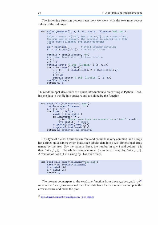
34 1 Algorithms and Implementations
The following function demonstrates how we work with the two most recentvalues of the unknown:
def solver_memsave(I, a, T, dt, theta, filename=’sol.dat’):"""Solve u’=-a*u, u(0)=I, for t in (0,T] with steps of dt.Minimum use of memory. The solution is stored in a file(with name filename) for later plotting."""dt = float(dt) # avoid integer divisionNt = int(round(T/dt)) # no of intervals
outfile = open(filename, ’w’)# u: time level n+1, u_1: time level nt = 0u_1 = Ioutfile.write(’%.16E %.16E\n’ % (t, u_1))for n in range(1, Nt+1):
u = (1 - (1-theta)*a*dt)/(1 + theta*dt*a)*u_1u_1 = ut += dtoutfile.write(’%.16E %.16E\n’ % (t, u))
outfile.close()return u, t
This code snippet also serves as a quick introduction to file writing in Python. Read-ing the data in the file into arrays t and u is done by the function
def read_file(filename=’sol.dat’):infile = open(filename, ’r’)u = []; t = []for line in infile:
words = line.split()if len(words) != 2:
print ’Found more than two numbers on a line!’, wordssys.exit(1) # abort
t.append(float(words[0]))u.append(float(words[1]))
return np.array(t), np.array(u)
This type of file with numbers in rows and columns is very common, and numpyhas a function loadtxt which loads such tabular data into a two-dimensional arraynamed by the user. Say the name is data, the number in row i and column j isthen data[i,j]. The whole column number j can be extracted by data[:,j].A version of read_file using np.loadtxt reads
def read_file_numpy(filename=’sol.dat’):data = np.loadtxt(filename)t = data[:,0]u = data[:,1]return t, u
The present counterpart to the explore function from decay_plot_mpl.py17
must run solver_memsave and then load data from file before we can compute theerror measure and make the plot:
17 http://tinyurl.com/ofkw6kc/alg/decay_plot_mpl.py

1.3 Exercises 35
def explore(I, a, T, dt, theta=0.5, makeplot=True):filename = ’u.dat’u, t = solver_memsave(I, a, T, dt, theta, filename)
t, u = read_file(filename)u_e = u_exact(t, I, a)e = u_e - uE = sqrt(dt*np.sum(e**2))if makeplot:
figure()...
Apart from the internal implementation, where un values are stored in a filerather than in an array, decay_memsave.py file works exactly as thedecay_plot_mpl.py file.
1.3 Exercises
Exercise 1.1: Define a mesh function and visualize it
a) Write a function mesh_function(f, t) that returns an array with mesh pointvalues f .t0/; : : : ; f .tNt
/, where f is a Python function implementing a mathe-matical function f(t) and t0; : : : ; tNt
are mesh points stored in the array t. Usea loop over the mesh points and compute one mesh function value at the time.
b) Use mesh_function to compute the mesh function corresponding to
f .t/ D(
e�t ; 0 � t � 3;
e�3t ; 3 < t � 4
Choose a mesh tn D n�t with �t D 0:1. Plot the mesh function.
Filename: mesh_function.
Remarks In Sect. 1.2.9 we show how easy it is to compute a mesh function byarray arithmetics (or array computing). Using this technique, one could simplyimplement mesh_function(f,t) as return f(t). However, f(t) will not workif there are if tests involving t inside f as is the case in b). Typically, if t < 3must have t < 3 as a boolean expression, but if t is array, t < 3, is an array ofboolean values, which is not legal as a boolean expression in an if test. Computingone element at a time as suggested in a) is a way of out of this problem.
We also remark that the function in b) is the solution of u0 D �au, u.0/ D 1,for t 2 Œ0; 4�, where a D 1 for t 2 Œ0; 3� and a D 3 for t 2 Œ3; 4�.
Problem 1.2: Differentiate a functionGiven a mesh function un as an array u with un values at mesh points tn D n�t ,the discrete derivative can be based on centered differences:
d n D ŒD2tu�n D unC1 � un�1
2�t; n D 1; : : : ; Nt � 1 : (1.58)

36 1 Algorithms and Implementations
At the end points we use forward and backward differences:
d 0 D ŒDCt u�n D u1 � u0
�t;
and
d Nt D ŒD�t u�n D uNt � uNt�1
�t:
a) Write a function differentiate(u, dt) that returns the discrete derivatived n of the mesh function un. The parameter dt reflects the mesh spacing �t .Write a corresponding test function test_differentiate() for verifying theimplementation.
Hint The three differentiation formulas are exact for quadratic polynomials. Usethis property to verify the program.
b) A standard implementation of the formula (1.58) is to have a loop over i . Forlarge Nt , such loop may run slowly in Python. A technique for speeding upthe computations, called vectorization or array computing, replaces the loopby array operations. To see how this can be done in the present mathematicalproblem, we define two arrays
uC D .u2; u3; : : : ; uNt /; u� D .u0; u1; : : : ; uNt�2/ :
The formula (1.58) can now be expressed as
.d 1; d 2; : : : ; d Nt�1/ D 1
2�t.uC � u�/ :
The corresponding Python code reads
d[1:-1] = (u[2:] - u[0:-2])/(2*dt)# ord[1:N_t] = (u[2:N_t+1] - u[0:N_t-1])/(2*dt)
Recall that an array slice u[1:-1] contains the elements in u starting with index1 and going all indices up to, but not including, the last one (-1).Use the ideas above to implement a vectorized version of the differentiatefunction without loops. Make a corresponding test function that compares theresult with that of differentiate.
Filename: differentiate.
Problem 1.3: Experiment with divisionsExplain what happens in the following computations, where some are mathemati-cally unexpected:

1.3 Exercises 37
>>> dt = 3>>> T = 8>>> Nt = T/dt>>> Nt2>>> theta = 1; a = 1>>> (1 - (1-theta)*a*dt)/(1 + theta*dt*a)0
Filename: pyproblems.
Problem 1.4: Experiment with wrong computationsConsider the solver function in the decay_v1.py18 file and the following call:
u, t = solver(I=1, a=1, T=7, dt=2, theta=1)
The output becomes
t= 0.000 u=1t= 2.000 u=0t= 4.000 u=0t= 6.000 u=0
Print out the result of all intermediate computations and use type(v) to see theobject type of the result stored in some variable v. Examine the intermediate cal-culations and explain why u is wrong and why we compute up to t D 6 only eventhough we specified T D 7.
Filename: decay_v1_err.
Problem 1.5: Plot the error functionSolve the problem u0 D �au, u.0/ D I , using the Forward Euler, BackwardEuler, and Crank–Nicolson schemes. For each scheme, plot the error mesh functionen D ue.tn/ � un for �t D 0:1; 0:05; 0:025, where ue is the exact solution of theODE and un is the numerical solution at mesh point tn.
Hint Modify the decay_plot_mpl.py19 code.Filename: decay_plot_error.
Problem 1.6: Change formatting of numbers and debugThe decay_memsave.py20 program writes the time values and solution values toa file which looks like
0.0000000000000000E+00 1.0000000000000000E+002.0000000000000001E-01 8.3333333333333337E-014.0000000000000002E-01 6.9444444444444453E-016.0000000000000009E-01 5.7870370370370383E-018.0000000000000004E-01 4.8225308641975323E-011.0000000000000000E+00 4.0187757201646102E-011.2000000000000000E+00 3.3489797668038418E-011.3999999999999999E+00 2.7908164723365347E-01
18 http://tinyurl.com/ofkw6kc/alg/decay_v1.py19 http://tinyurl.com/ofkw6kc/alg/decay_plot_mpl.py20 http://tinyurl.com/ofkw6kc/alg/decay_memsave.py

38 1 Algorithms and Implementations
Modify the file output such that it looks like
0.000 1.000000.200 0.833330.400 0.694440.600 0.578700.800 0.482251.000 0.401881.200 0.334901.400 0.27908
If you have just modified the formatting of numbers in the file, running the modifiedprogram
Terminal
Terminal> python decay_memsave_v2.py --T 10 --theta 1 \--dt 0.2 --makeplot
leads to printing of the message Bug in the implementation! in the terminalwindow. Why?
Filename: decay_memsave_v2.
Open Access This chapter is distributed under the terms of the Creative Commons Attribution-NonCommercial 4.0 International License (http://creativecommons.org/licenses/by-nc/4.0/),which permits any noncommercial use, duplication, adaptation, distribution and reproductionin any medium or format, as long as you give appropriate credit to the original author(s) and thesource, a link is provided to the Creative Commons license and any changes made are indicated.
The images or other third party material in this chapter are included in the work’s CreativeCommons license, unless indicated otherwise in the credit line; if such material is not includedin the work’s Creative Commons license and the respective action is not permitted by statutoryregulation, users will need to obtain permission from the license holder to duplicate, adapt orreproduce the material.

2Analysis
We address the ODE for exponential decay,
u0.t/ D �au.t/; u.0/ D I; (2.1)
where a and I are given constants. This problem is solved by the �-rule finitedifference scheme, resulting in the recursive equations
unC1 D 1 � .1 � �/a�t
1C �a�tun (2.2)
for the numerical solution unC1, which approximates the exact solution ue at timepoint tnC1. For constant mesh spacing, which we assume here, tnC1 D .nC 1/�t .
The example programs associated with this chapter are found in the directorysrc/analysis1.
2.1 Experimental Investigations
We first perform a series of numerical explorations to see how the methods behaveas we change the parameters I , a, and �t in the problem.
2.1.1 Discouraging Numerical Solutions
Choosing I D 1, a D 2, and running experiments with � D 1; 0:5; 0 for �t D1:25; 0:75; 0:5; 0:1, gives the results in Figs. 2.1, 2.2, and 2.3.
The characteristics of the displayed curves can be summarized as follows:
� The Backward Euler scheme gives a monotone solution in all cases, lying abovethe exact curve.
� The Crank–Nicolson scheme gives the most accurate results, but for �t D 1:25
the solution oscillates.
1 http://tinyurl.com/ofkw6kc/analysis
39© The Author(s) 2016H.P. Langtangen, Finite Difference Computing with Exponential Decay Models,Lecture Notes in Computational Science and Engineering 110,DOI 10.1007/978-3-319-29439-1_2

40 2 Analysis
Fig. 2.1 Backward Euler
� The Forward Euler scheme gives a growing, oscillating solution for �t D 1:25;a decaying, oscillating solution for �t D 0:75; a strange solution un D 0 forn 1 when �t D 0:5; and a solution seemingly as accurate as the one bythe Backward Euler scheme for �t D 0:1, but the curve lies below the exactsolution.
Since the exact solution of our model problem is a monotone function, u.t/ DIe�at , some of these qualitatively wrong results indeed seem alarming!
Key questions� Under what circumstances, i.e., values of the input data I , a, and �t will the
Forward Euler and Crank–Nicolson schemes result in undesired oscillatorysolutions?
� How does �t impact the error in the numerical solution?
The first question will be investigated both by numerical experiments and byprecise mathematical theory. The theory will help establish general criteria on�t for avoiding non-physical oscillatory or growing solutions.
For our simple model problem we can answer the second question very pre-cisely, but we will also look at simplified formulas for small �t and touch upon
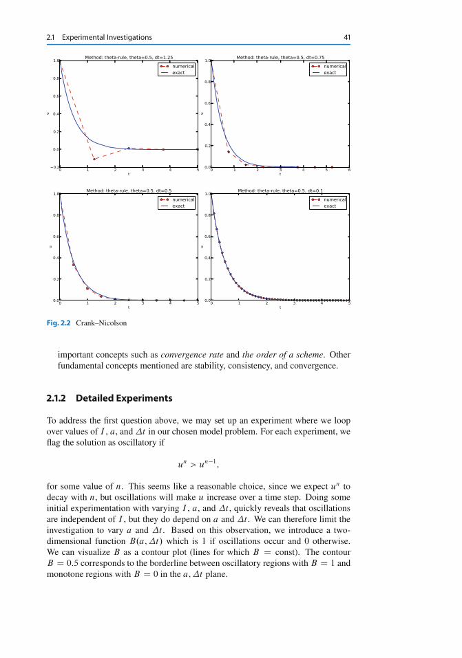
2.1 Experimental Investigations 41
Fig. 2.2 Crank–Nicolson
important concepts such as convergence rate and the order of a scheme. Otherfundamental concepts mentioned are stability, consistency, and convergence.
2.1.2 Detailed Experiments
To address the first question above, we may set up an experiment where we loopover values of I , a, and �t in our chosen model problem. For each experiment, weflag the solution as oscillatory if
un > un�1;
for some value of n. This seems like a reasonable choice, since we expect un todecay with n, but oscillations will make u increase over a time step. Doing someinitial experimentation with varying I , a, and �t , quickly reveals that oscillationsare independent of I , but they do depend on a and �t . We can therefore limit theinvestigation to vary a and �t . Based on this observation, we introduce a two-dimensional function B.a; �t/ which is 1 if oscillations occur and 0 otherwise.We can visualize B as a contour plot (lines for which B D const). The contourB D 0:5 corresponds to the borderline between oscillatory regions with B D 1 andmonotone regions with B D 0 in the a; �t plane.

42 2 Analysis
Fig. 2.3 Forward Euler
The B function is defined at discrete a and �t values. Say we have given P
values for a, a0; : : : ; aP�1, and Q values for �t , �t0; : : : ; �tQ�1. These ai and�tj values, i D 0; : : : ; P � 1, j D 0; : : : ; Q � 1, form a rectangular mesh ofP Q points in the plane spanned by a and �t . At each point .ai ; �tj /, weassociate the corresponding value B.ai ; �tj /, denoted Bij . The Bij values are nat-urally stored in a two-dimensional array. We can thereafter create a plot of thecontour line Bij D 0:5 dividing the oscillatory and monotone regions. The filedecay_osc_regions.py2 given below (osc_regions stands for “oscillatory re-gions”) contains all nuts and bolts to produce the B D 0:5 line in Figs. 2.4 and 2.5.The oscillatory region is above this line.
from decay_mod import solverimport numpy as npimport scitools.std as st
def non_physical_behavior(I, a, T, dt, theta):"""Given lists/arrays a and dt, and numbers I, dt, and theta,make a two-dimensional contour line B=0.5, where B=1>0.5means oscillatory (unstable) solution, and B=0<0.5 meansmonotone solution of u’=-au."""
2 http://tinyurl.com/ofkw6kc/analysis/decay_osc_regions.py

2.1 Experimental Investigations 43
Fig. 2.4 Forward Euler scheme: oscillatory solutions occur for points above the curve
a = np.asarray(a); dt = np.asarray(dt) # must be arraysB = np.zeros((len(a), len(dt))) # resultsfor i in range(len(a)):
for j in range(len(dt)):u, t = solver(I, a[i], T, dt[j], theta)# Does u have the right monotone decay properties?correct_qualitative_behavior = Truefor n in range(1, len(u)):
if u[n] > u[n-1]: # Not decaying?correct_qualitative_behavior = Falsebreak # Jump out of loop
B[i,j] = float(correct_qualitative_behavior)a_, dt_ = st.ndgrid(a, dt) # make mesh of a and dt valuesst.contour(a_, dt_, B, 1)st.grid(’on’)st.title(’theta=%g’ % theta)st.xlabel(’a’); st.ylabel(’dt’)st.savefig(’osc_region_theta_%s.png’ % theta)st.savefig(’osc_region_theta_%s.pdf’ % theta)
non_physical_behavior(I=1,a=np.linspace(0.01, 4, 22),dt=np.linspace(0.01, 4, 22),T=6,theta=0.5)
By looking at the curves in the figures one may guess that a�t must be lessthan a critical limit to avoid the undesired oscillations. This limit seems to be about2 for Crank–Nicolson and 1 for Forward Euler. We shall now establish a precisemathematical analysis of the discrete model that can explain the observations in ournumerical experiments.

44 2 Analysis
Fig. 2.5 Crank–Nicolson scheme: oscillatory solutions occur for points above the curve
2.2 Stability
The goal now is to understand the results in the previous section. To this end, weshall investigate the properties of the mathematical formula for the solution of theequations arising from the finite difference methods.
2.2.1 Exact Numerical Solution
Starting with u0 D I , the simple recursion (2.2) can be applied repeatedly n times,with the result that
un D IAn; A D 1 � .1 � �/a�t
1C �a�t: (2.3)
Solving difference equationsDifference equations where all terms are linear in unC1, un, and maybe un�1,un�2, etc., are called homogeneous, linear difference equations, and their solu-tions are generally of the form un D An, where A is a constant to be determined.Inserting this expression in the difference equation and dividing by AnC1 givesa polynomial equation in A. In the present case we get
A D 1 � .1 � �/a�t
1C �a�t:
This is a solution technique of wider applicability than repeated use of the recur-sion (2.2).

2.2 Stability 45
Regardless of the solution approach, we have obtained a formula for un. Thisformula can explain everything we see in the figures above, but it also gives usa more general insight into accuracy and stability properties of the three schemes.
Since un is a factor A raised to an integer power n, we realize that A < 0 willimply un < 0 for odd n and un > 0 for even n. That is, the solution oscillatesbetween the mesh points. We have oscillations due to A < 0 when
.1 � �/a�t > 1 : (2.4)
Since A > 0 is a requirement for having a numerical solution with the same basicproperty (monotonicity) as the exact solution, we may say that A > 0 is a stabilitycriterion. Expressed in terms of �t the stability criterion reads
�t <1
.1 � �/a: (2.5)
The Backward Euler scheme is always stable since A < 0 is impossible for� D 1, while non-oscillating solutions for Forward Euler and Crank–Nicolson de-mand �t � 1=a and �t � 2=a, respectively. The relation between �t and a lookreasonable: a larger a means faster decay and hence a need for smaller time steps.
Looking at the upper left plot in Fig. 2.3, we see that �t D 1:25, and remember-ing that a D 2 in these experiments, A can be calculated to be�1:5, so the ForwardEuler solution becomes un D .�1:5/n (I D 1). This solution oscillates and grows.The upper right plot has a�t D 2 � 0:75 D 1:5, so A D �0:5, and un D .�0:5/n
decays but oscillates. The lower left plot is a peculiar case where the Forward Eulerscheme produces a solution that is stuck on the t axis. Now we can understand whythis is so, because a�t D 2 � 0:5 D 1, which gives A D 0, and therefore un D 0 forn 1. The decaying oscillations in the Crank–Nicolson scheme in the upper leftplot in Fig. 2.2 for �t D 1:25 are easily explained by the fact that A � �0:11 < 0.
2.2.2 Stability Properties Derived from the Amplification Factor
The factor A is called the amplification factor since the solution at a new timelevel is the solution at the previous time level amplified by a factor A. For a decayprocess, we must obviously have jAj � 1, which is fulfilled for all �t if � 1=2.Arbitrarily large values of u can be generated when jAj > 1 and n is large enough.The numerical solution is in such cases totally irrelevant to an ODE modeling decayprocesses! To avoid this situation, we must demand jAj � 1 also for � < 1=2,which implies
�t � 2
.1 � 2�/a; (2.6)
For example, �t must not exceed 2=a when computing with the Forward Eulerscheme.

46 2 Analysis
Stability propertiesWe may summarize the stability investigations as follows:
1. The Forward Euler method is a conditionally stable scheme because it re-quires �t < 2=a for avoiding growing solutions and �t < 1=a for avoidingoscillatory solutions.
2. The Crank–Nicolson is unconditionally stable with respect to growing solu-tions, while it is conditionally stable with the criterion �t < 2=a for avoidingoscillatory solutions.
3. The Backward Euler method is unconditionally stable with respect to grow-ing and oscillatory solutions – any �t will work.
Much literature on ODEs speaks about L-stable and A-stable methods. In ourcase A-stable methods ensures non-growing solutions, while L-stable methodsalso avoids oscillatory solutions.
2.3 Accuracy
While stability concerns the qualitative properties of the numerical solution, it re-mains to investigate the quantitative properties to see exactly how large the numer-ical errors are.
2.3.1 Visual Comparison of Amplification Factors
After establishing how A impacts the qualitative features of the solution, we shallnow look more into how well the numerical amplification factor approximates theexact one. The exact solution reads u.t/ D Ie�at , which can be rewritten as
ue.tn/ D Ie�an�t D I.e�a�t /n : (2.7)
From this formula we see that the exact amplification factor is
Ae D e�a�t : (2.8)
We see from all of our analysis that the exact and numerical amplification factorsdepend on a and �t through the dimensionless product a�t : whenever there isa �t in the analysis, there is always an associated a parameter. Therefore, it isconvenient to introduce a symbol for this product, p D a�t , and view A and Ae asfunctions of p. Figure 2.6 shows these functions. The two amplification factors areclearly closest for the Crank–Nicolson method, but that method has the unfortunateoscillatory behavior when p > 2.
Significance of the p D a�t parameterThe key parameter for numerical performance of a scheme is in this model prob-lem p D a�t . This is a dimensionless number (a has dimension 1/s and �t

2.3 Accuracy 47
Fig. 2.6 Comparison of amplification factors
has dimension s) reflecting how the discretization parameter plays together witha physical parameter in the problem.
One can bring the present model problem on dimensionless form througha process called scaling. The scaled modeled has a modified time Nt D at andmodified response Nu D u=I such that the model reads d Nu=d Nt D �Nu, Nu.0/ D 1.Analyzing this model, where there are no physical parameters, we find that �Ntis the key parameter for numerical performance. In the unscaled model, thiscorresponds to �Nt D a�t .
It is common that the numerical performance of methods for solving ordinaryand partial differential equations is governed by dimensionless parameters thatcombine mesh sizes with physical parameters.
2.3.2 Series Expansion of Amplification Factors
As an alternative to the visual understanding inherent in Fig. 2.6, there is a strongtradition in numerical analysis to establish formulas for approximation errors whenthe discretization parameter, here �t , becomes small. In the present case, we let p
be our small discretization parameter, and it makes sense to simplify the expressionsfor A and Ae by using Taylor polynomials around p D 0. The Taylor polynomi-als are accurate for small p and greatly simplify the comparison of the analyticalexpressions since we then can compare polynomials, term by term.
Calculating the Taylor series for Ae is easily done by hand, but the three versionsof A for � D 0; 1; 1
2lead to more cumbersome calculations. Nowadays, analyti-
cal computations can benefit greatly by symbolic computer algebra software. ThePython package sympy represents a powerful computer algebra system, not yet assophisticated as the famous Maple and Mathematica systems, but it is free and veryeasy to integrate with our numerical computations in Python.

48 2 Analysis
When using sympy, it is convenient to enter an interactive Python shell where theresults of expressions and statements can be shown immediately. Here is a simpleexample. We strongly recommend to use isympy (or ipython) for such interactivesessions.
Let us illustrate sympy with a standard Python shell syntax (»> prompt) to com-pute a Taylor polynomial approximation to e�p:
>>> from sympy import *>>> # Create p as a mathematical symbol with name ’p’>>> p = Symbols(’p’)>>> # Create a mathematical expression with p>>> A_e = exp(-p)>>>>>> # Find the first 6 terms of the Taylor series of A_e>>> A_e.series(p, 0, 6)1 + (1/2)*p**2 - p - 1/6*p**3 - 1/120*p**5 + (1/24)*p**4 + O(p**6)
Lines with »> represent input lines, whereas without this prompt represent the resultof the previous command (note that isympy and ipython apply other prompts, butin this text we always apply »> for interactive Python computing). Apart from theorder of the powers, the computed formula is easily recognized as the beginning ofthe Taylor series for e�p .
Let us define the numerical amplification factor where p and � enter the formulaas symbols:
>>> theta = Symbol(’theta’)>>> A = (1-(1-theta)*p)/(1+theta*p)
To work with the factor for the Backward Euler scheme we can substitute the value1 for theta:
>>> A.subs(theta, 1)1/(1 + p)
Similarly, we can substitute theta by 1=2 for Crank–Nicolson, preferably using anexact rational representation of 1=2 in sympy:
>>> half = Rational(1,2)>>> A.subs(theta, half)1/(1 + (1/2)*p)*(1 - 1/2*p)
The Taylor series of the amplification factor for the Crank–Nicolson scheme canbe computed as
>>> A.subs(theta, half).series(p, 0, 4)1 + (1/2)*p**2 - p - 1/4*p**3 + O(p**4)

2.3 Accuracy 49
We are now in a position to compare Taylor series:
>>> FE = A_e.series(p, 0, 4) - A.subs(theta, 0).series(p, 0, 4)>>> BE = A_e.series(p, 0, 4) - A.subs(theta, 1).series(p, 0, 4)>>> CN = A_e.series(p, 0, 4) - A.subs(theta, half).series(p, 0, 4 )>>> FE(1/2)*p**2 - 1/6*p**3 + O(p**4)>>> BE-1/2*p**2 + (5/6)*p**3 + O(p**4)>>> CN(1/12)*p**3 + O(p**4)
From these expressions we see that the error A � Ae � O.p2/ for the Forward andBackward Euler schemes, while A�Ae � O.p3/ for the Crank–Nicolson scheme.The notation O.pm/ here means a polynomial in p where pm is the term of lowest-degree, and consequently the term that dominates the expression for p < 0. We callthis the leading order term. As p ! 0, the leading order term clearly dominatesover the higher-order terms (think of p D 0:01: p is a hundred times larger than p2).
Now, a is a given parameter in the problem, while �t is what we can vary. Notsurprisingly, the error expressions are usually written in terms �t . We then have
A � Ae D(O.�t2/; Forward and Backward Euler;
O.�t3/; Crank–Nicolson(2.9)
We say that the Crank–Nicolson scheme has an error in the amplification factorof order �t3, while the two other schemes are of order �t2 in the same quantity.
What is the significance of the order expression? If we halve �t , the error in am-plification factor at a time level will be reduced by a factor of 4 in the Forward andBackward Euler schemes, and by a factor of 8 in the Crank–Nicolson scheme. Thatis, as we reduce �t to obtain more accurate results, the Crank–Nicolson schemereduces the error more efficiently than the other schemes.
2.3.3 The Ratio of Numerical and Exact Amplification Factors
An alternative comparison of the schemes is provided by looking at the ratio A=Ae,or the error 1 � A=Ae in this ratio:
>>> FE = 1 - (A.subs(theta, 0)/A_e).series(p, 0, 4)>>> BE = 1 - (A.subs(theta, 1)/A_e).series(p, 0, 4)>>> CN = 1 - (A.subs(theta, half)/A_e).series(p, 0, 4)>>> FE(1/2)*p**2 + (1/3)*p**3 + O(p**4)>>> BE-1/2*p**2 + (1/3)*p**3 + O(p**4)>>> CN(1/12)*p**3 + O(p**4)
The leading-order terms have the same powers as in the analysis of A � Ae.
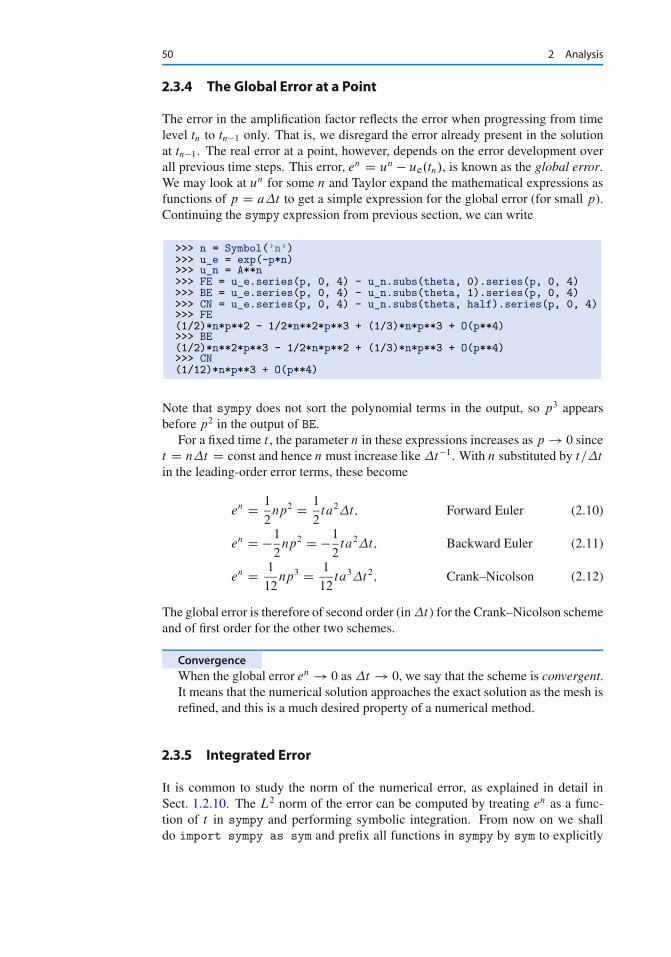
50 2 Analysis
2.3.4 The Global Error at a Point
The error in the amplification factor reflects the error when progressing from timelevel tn to tn�1 only. That is, we disregard the error already present in the solutionat tn�1. The real error at a point, however, depends on the error development overall previous time steps. This error, en D un � ue.tn/, is known as the global error.We may look at un for some n and Taylor expand the mathematical expressions asfunctions of p D a�t to get a simple expression for the global error (for small p).Continuing the sympy expression from previous section, we can write
>>> n = Symbol(’n’)>>> u_e = exp(-p*n)>>> u_n = A**n>>> FE = u_e.series(p, 0, 4) - u_n.subs(theta, 0).series(p, 0, 4)>>> BE = u_e.series(p, 0, 4) - u_n.subs(theta, 1).series(p, 0, 4)>>> CN = u_e.series(p, 0, 4) - u_n.subs(theta, half).series(p, 0, 4)>>> FE(1/2)*n*p**2 - 1/2*n**2*p**3 + (1/3)*n*p**3 + O(p**4)>>> BE(1/2)*n**2*p**3 - 1/2*n*p**2 + (1/3)*n*p**3 + O(p**4)>>> CN(1/12)*n*p**3 + O(p**4)
Note that sympy does not sort the polynomial terms in the output, so p3 appearsbefore p2 in the output of BE.
For a fixed time t , the parameter n in these expressions increases as p ! 0 sincet D n�t D const and hence n must increase like �t�1. With n substituted by t=�t
in the leading-order error terms, these become
en D 1
2np2 D 1
2ta2�t; Forward Euler (2.10)
en D �1
2np2 D �1
2ta2�t; Backward Euler (2.11)
en D 1
12np3 D 1
12ta3�t2; Crank–Nicolson (2.12)
The global error is therefore of second order (in �t) for the Crank–Nicolson schemeand of first order for the other two schemes.
ConvergenceWhen the global error en ! 0 as �t ! 0, we say that the scheme is convergent.It means that the numerical solution approaches the exact solution as the mesh isrefined, and this is a much desired property of a numerical method.
2.3.5 Integrated Error
It is common to study the norm of the numerical error, as explained in detail inSect. 1.2.10. The L2 norm of the error can be computed by treating en as a func-tion of t in sympy and performing symbolic integration. From now on we shalldo import sympy as sym and prefix all functions in sympy by sym to explicitly

2.3 Accuracy 51
notify ourselves that the functions are from sympy. This is particularly advanta-geous when we use mathematical functions like sin: sym.sin is for symbolicexpressions, while sin from numpy or math is for numerical computation. For theForward Euler scheme we have
import sympy as symp, n, a, dt, t, T, theta = sym.symbols(’p n a dt t T theta’)A = (1-(1-theta)*p)/(1+theta*p)u_e = sym.exp(-p*n)u_n = A**nerror = u_e.series(p, 0, 4) - u_n.subs(theta, 0).series(p, 0, 4)# Introduce t and dt instead of n and perror = error.subs(’n’, ’t/dt’).subs(p, ’a*dt’)error = error.as_leading_term(dt) # study only the first termprint errorerror_L2 = sym.sqrt(sym.integrate(error**2, (t, 0, T)))print ’L2 error:’, sym.simplify(error_error_L2)
The output reads
sqrt(30)*sqrt(T**3*a**4*dt**2*(6*T**2*a**2 - 15*T*a + 10))/60
which means that the L2 error behaves like a2�t .Strictly speaking, the numerical error is only defined at the mesh points so it
makes most sense to compute the `2 error
jjenjj`2 Dvuut�t
NtXnD0
.ue.tn/� un/2 :
We have obtained an exact analytical expression for the error at t D tn, but here weuse the leading-order error term only since we are mostly interested in how the errorbehaves as a polynomial in �t or p, and then the leading order term will dominate.For the Forward Euler scheme, ue.tn/ � un � 1
2np2, and we have
jjenjj2`2 D �t
NtXnD0
1
4n2p4 D �t
1
4p4
NtXnD0
n2 :
Now,PNt
nD0 n2 � 13N 3
t . Using this approximation, setting Nt D T=�t , and takingthe square root gives the expression
jjenjj`2 D 1
2
rT 3
3a2�t : (2.13)
Calculations for the Backward Euler scheme are very similar and provide the sameresult, while the Crank–Nicolson scheme leads to
jjenjj`2 D 1
12
rT 3
3a3�t2 : (2.14)

52 2 Analysis
Summary of errorsBoth the global point-wise errors (2.10)–(2.12) and their time-integrated versions(2.13) and (2.14) show that
� the Crank–Nicolson scheme is of second order in �t , and� the Forward Euler and Backward Euler schemes are of first order in �t .
2.3.6 Truncation Error
The truncation error is a very frequently used error measure for finite differencemethods. It is defined as the error in the difference equation that arises when in-serting the exact solution. Contrary to many other error measures, e.g., the trueerror en D ue.tn/ � un, the truncation error is a quantity that is easily computable.
Before reading on, it is wise to review Sect. 1.1.7 on how Taylor polynomialswere used to derive finite differences and quantify the error in the formulas. Verysimilar reasoning, and almost identical mathematical details, will be carried outbelow, but in a slightly different context. Now, the focus is on the error when solvinga differential equation, while in Sect. 1.1.7 we derived errors for a finite differenceformula. These errors are tightly connected in the present model problem.
Let us illustrate the calculation of the truncation error for the Forward Eulerscheme. We start with the difference equation on operator form,
ŒDCt u D �au�n;
which is the short form for
unC1 � un
�tD �aun :
The idea is to see how well the exact solution ue.t/ fulfills this equation. Sinceue.t/ in general will not obey the discrete equation, we get an error in the discreteequation. This error is called a residual, denoted here by Rn:
Rn D ue.tnC1/� ue.tn/
�tC aue.tn/ : (2.15)
The residual is defined at each mesh point and is therefore a mesh function witha superscript n.
The interesting feature of Rn is to see how it depends on the discretization pa-rameter �t . The tool for reaching this goal is to Taylor expand ue around the pointwhere the difference equation is supposed to hold, here t D tn. We have that
ue.tnC1/ D ue.tn/C u0e.tn/�t C 1
2u00e.tn/�t2 C � � � ;

2.3 Accuracy 53
which may be used to reformulate the fraction in (2.15) so that
Rn D u0e.tn/C 1
2u00e.tn/�t C : : :C aue.tn/ :
Now, ue fulfills the ODE u0e D �aue, which means that the first and last termcancel and we have
Rn D 1
2u00e.tn/�t CO.�t2/ :
This Rn is the truncation error, which for the Forward Euler is seen to be of firstorder in �t as �! 0.
The above procedure can be repeated for the Backward Euler and the Crank–Nicolson schemes. We start with the scheme in operator notation, write it out indetail, Taylor expand ue around the point Qt at which the difference equation isdefined, collect terms that correspond to the ODE (here u0e C aue), and identifythe remaining terms as the residual R, which is the truncation error. The BackwardEuler scheme leads to
Rn � �1
2u00e.tn/�t;
while the Crank–Nicolson scheme gives
RnC 12 � 1
24u000e .tnC 1
2/�t2;
when �t ! 0.The order r of a finite difference scheme is often defined through the leading
term �tr in the truncation error. The above expressions point out that the Forwardand Backward Euler schemes are of first order, while Crank–Nicolson is of secondorder. We have looked at other error measures in other sections, like the error inamplification factor and the error en D ue.tn/ � un, and expressed these errormeasures in terms of �t to see the order of the method. Normally, calculating thetruncation error is more straightforward than deriving the expressions for other errormeasures and therefore the easiest way to establish the order of a scheme.
2.3.7 Consistency, Stability, and Convergence
Three fundamental concepts when solving differential equations by numericalmethods are consistency, stability, and convergence. We shall briefly touch uponthese concepts below in the context of the present model problem.
Consistency means that the error in the difference equation, measured throughthe truncation error, goes to zero as �t ! 0. Since the truncation error tellshow well the exact solution fulfills the difference equation, and the exact solutionfulfills the differential equation, consistency ensures that the difference equationapproaches the differential equation in the limit. The expressions for the truncationerrors in the previous section are all proportional to �t or �t2, hence they vanishas �t ! 0, and all the schemes are consistent. Lack of consistency implies that weactually solve some other differential equation in the limit �t ! 0 than we aim at.

54 2 Analysis
Stability means that the numerical solution exhibits the same qualitative proper-ties as the exact solution. This is obviously a feature we want the numerical solutionto have. In the present exponential decay model, the exact solution is monotone anddecaying. An increasing numerical solution is not in accordance with the decayingnature of the exact solution and hence unstable. We can also say that an oscillat-ing numerical solution lacks the property of monotonicity of the exact solution andis also unstable. We have seen that the Backward Euler scheme always leads tomonotone and decaying solutions, regardless of �t , and is hence stable. The For-ward Euler scheme can lead to increasing solutions and oscillating solutions if �t
is too large and is therefore unstable unless �t is sufficiently small. The Crank–Nicolson can never lead to increasing solutions and has no problem to fulfill thatstability property, but it can produce oscillating solutions and is unstable in thatsense, unless �t is sufficiently small.
Convergence implies that the global (true) error mesh function en D ue.tn/ �un ! 0 as �t ! 0. This is really what we want: the numerical solution gets asclose to the exact solution as we request by having a sufficiently fine mesh.
Convergence is hard to establish theoretically, except in quite simple problemslike the present one. Stability and consistency are much easier to calculate. A majorbreakthrough in the understanding of numerical methods for differential equationscame in 1956 when Lax and Richtmeyer established equivalence between conver-gence on one hand and consistency and stability on the other (the Lax equivalencetheorem3). In practice it meant that one can first establish that a method is stableand consistent, and then it is automatically convergent (which is much harder toestablish). The result holds for linear problems only, and in the world of nonlineardifferential equations the relations between consistency, stability, and convergenceare much more complicated.
We have seen in the previous analysis that the Forward Euler, Backward Euler,and Crank–Nicolson schemes are convergent (en ! 0), that they are consistent(Rn ! 0), and that they are stable under certain conditions on the size of �t . Wehave also derived explicit mathematical expressions for en, the truncation error, andthe stability criteria.
2.4 Various Types of Errors in a Differential Equation Model
So far we have been concerned with one type of error, namely the discretizationerror committed by replacing the differential equation problem by a recursive setof difference equations. There are, however, other types of errors that must beconsidered too. We can classify errors into four groups:
1. model errors: how wrong is the ODE model?2. data errors: how wrong are the input parameters?3. discretization errors: how wrong is the numerical method?4. rounding errors: how wrong is the computer arithmetics?
Below, we shall briefly describe and illustrate these four types of errors. Each ofthe errors deserve its own chapter, at least, so the treatment here is superficial to
3 http://en.wikipedia.org/wiki/Lax_equivalence_theorem

2.4 Various Types of Errors in a Differential EquationModel 55
give some indication about the nature of size of the errors in a specific case. Someof the required computer codes quickly become more advanced than in the rest ofthe book, but we include to code to document all the details that lie behind theinvestigations of the errors.
2.4.1 Model Errors
Any mathematical modeling like u0 D �au, u.0/ D I , is just an approximatedescription of a real-world phenomenon. How good this approximation is can bedetermined by comparing physical experiments with what the model predicts. Thisis the topic of validation and is obviously an essential part of mathematical mod-eling. One difficulty with validation is that we need to estimate the parameters inthe model, and this brings in data errors. Quantifying data errors is challenging,and a frequently used method is to tune the parameters in the model to make modelpredictions as close as possible to the experiments. That is, we do not attempt tomeasure or estimate all input parameters, but instead find values that “make themodel good”. Another difficulty is that the response in experiments also containserrors due to measurement techniques.
Let us try to quantify model errors in a very simple example involving u0 D �au,u.0/ D I , with constant a. Suppose a more accurate model has a as a function oftime rather than a constant. Here we take a.t/ as a simple linear function: a C pt .Obviously, u with p > 0 will go faster to zero with time than a constant a.
The solution ofu0 D .aC pt/u; u.0/ D I;
can be shown (see below) to be
u.t/ D Ie�t.aC 12 pt/ :
Let a Python function true_model(t, I, a, p) implement the above u.t/
and let the solution of our primary ODE u0 D �au be available as the functionmodel(t, I, a). We can now make some plots of the two models and theerror for some values of p. Figure 2.7 displays model versus true_model forp D 0:01; 0:1; 1, while Fig. 2.8 shows the difference between the two models asa function of t for the same p values.
The code that was used to produce the plots looks like
from numpy import linspace, expfrom matplotlib.pyplot import \
plot, show, xlabel, ylabel, legend, savefig, figure, title
def model_errors():p_values = [0.01, 0.1, 1]a = 1I = 1t = linspace(0, 4, 101)legends = []# Work with figure(1) for the discrepancy and figure(2+i)# for plotting the model and the true model for p value no ifor i, p in enumerate(p_values):
u = model(t, I, a)

56 2 Analysis
Fig. 2.7 Comparison of two models for three values of p

2.4 Various Types of Errors in a Differential EquationModel 57
Fig. 2.8 Discrepancy of Comparison of two models for three values of p
u_true = true_model(t, I, a, p)discrepancy = u_true - ufigure(1)plot(t, discrepancy)figure(2+i)plot(t, u, ’r-’, t, u_true, ’b--’)legends.append(’p=%g’ % p)
figure(1)legend(legends, loc=’lower right’)savefig(’tmp1.png’); savefig(’tmp1.pdf’)for i, p in enumerate(p_values):
figure(2+i)legend([’model’, ’true model’])title(’p=%g’ % p)savefig(’tmp%d.png’ % (2+i)); savefig(’tmp%d.pdf’ % (2+i))
To derive the analytical solution of the model u0 D �.a C pt/u, u.0/ D I , wecan use SymPy and the code below. This is somewhat advanced SymPy use fora newbie, but serves to illustrate the possibilities to solve differential equations bysymbolic software.
def derive_true_solution():import sympy as symu = sym.symbols(’u’, cls=sym.Function) # function u(t)t, a, p, I = sym.symbols(’t a p I’, real=True)
def ode(u, t, a, p):"""Define ODE: u’ = (a + p*t)*u. Return residual."""return sym.diff(u, t) + (a + p*t)*u
eq = ode(u(t), t, a, p)s = sym.dsolve(eq)# s is sym.Eq object u(t) == expression, we want u = expression,# so grab the right-hand side of the equality (Eq obj.)u = s.rhsprint u

58 2 Analysis
# u contains C1, replace it with a symbol we can fit to# the initial conditionC1 = sym.symbols(’C1’, real=True)u = u.subs(’C1’, C1)print u# Initial condition equationeq = u.subs(t, 0) - Is = sym.solve(eq, C1) # solve eq wrt C1print s# s is a list s[0] = ...# Replace C1 in u by the solutionu = u.subs(C1, s[0])print ’u:’, uprint sym.latex(u) # latex formula for reports
# Consistency check: u must fulfill ODE and initial conditionprint ’ODE is fulfilled:’, sym.simplify(ode(u, t, a, p))print ’u(0)-I:’, sym.simplify(u.subs(t, 0) - I)
# Convert u expression to Python numerical function# (modules=’numpy’ allows numpy arrays as arguments,# we want this for t)u_func = sym.lambdify([t, I, a, p], u, modules=’numpy’)return u_func
true_model = derive_true_solution()
2.4.2 Data Errors
By “data” we mean all the input parameters to a model, in our case I and a. Thevalues of these may contain errors, or at least uncertainty. Suppose I and a aremeasured from some physical experiments. Ideally, we have many samples of I
and a and from these we can fit probability distributions. Assume that I turnsout to be normally distributed with mean 1 and standard deviation 0.2, while a isuniformly distributed in the interval Œ0:5; 1:5�.
How will the uncertainty in I and a propagate through the model u D Ie�at ?That is, what is the uncertainty in u at a particular time t? This answer can easilybe answered using Monte Carlo simulation. It means that we draw a lot of samplesfrom the distributions for I and a. For each combination of I and a sample wecompute the corresponding u value for selected values of t . Afterwards, we can foreach selected t values make a histogram of all the computed u values to see what thedistribution of u values look like. Figure 2.9 shows the histograms correspondingto t D 0; 1; 3. We see that the distribution of u values is much like a symmetricnormal distribution at t D 0, centered around u D 1. At later times, the distributiongets more asymmetric and narrower. It means that the uncertainty decreases withtime.
From the computed u values we can easily calculate the mean and standard de-viation. The table below shows the mean and standard deviation values along withthe value if we just use the formula u D Ie�at with the mean values of I and a:I D 1 and a D 1. As we see, there is some discrepancy between this latter (naive)computation and the mean value produced by Monte Carlo simulation.

2.4 Various Types of Errors in a Differential EquationModel 59
time mean st.dev. u.t I I D a D 1/
0 1.00 0.200 1.001 0.38 0.135 0.373 0.07 0.060 0.14
Actually, u.t I I; a/ becomes a stochastic variable for each t when I and a arestochastic variables, as they are in the above Monte Carlo simulation. The meanof the stochastic u.t I I; a/ is not equal to u with mean values of the input data,u.t I I D a D 1/, unless u is linear in I and a (here u is nonlinear in a).
Estimating statistical uncertainty in input data and investigating how this uncer-tainty propagates to uncertainty in the response of a differential equation model(or other models) are key topics in the scientific field called uncertainty quantifica-tion, simply known as UQ. Estimation of the statistical properties of input data caneither be done directly from physical experiments, or one can find the parametervalues that provide a “best fit” of model predictions with experiments. Monte Carlosimulation is a general and widely used tool to solve the associated statistical prob-lems. The accuracy of the Monte Carlo results increases with increasing number ofsamples N , typically the error behaves like N �1=2.
The computer code required to do the Monte Carlo simulation and produce theplots in Fig. 2.9 is shown below.
def data_errors():from numpy import random, mean, stdfrom matplotlib.pyplot import histN = 10000# Draw random numbers for I and aI_values = random.normal(1, 0.2, N)a_values = random.uniform(0.5, 1.5, N)# Compute corresponding u values for some t valuest = [0, 1, 3]u_values = {} # samples for various t valuesu_mean = {}u_std = {}for t_ in t:
# Compute u samples corresponding to I and a samplesu_values[t_] = [model(t_, I, a)
for I, a in zip(I_values, a_values)]u_mean[t_] = mean(u_values[t_])u_std[t_] = std(u_values[t_])
figure()dummy1, bins, dummy2 = hist(
u_values[t_], bins=30, range=(0, I_values.max()),normed=True, facecolor=’green’)
#plot(bins)title(’t=%g’ % t_)savefig(’tmp_%g.png’ % t_); savefig(’tmp_%g.pdf’ % t_)
# Table of mean and standard deviation valuesprint ’time mean st.dev.’for t_ in t:
print ’%3g %.2f %.3f’ % (t_, u_mean[t_], u_std[t_])

60 2 Analysis
Fig. 2.9 Histogram of solution uncertainty at three time points, due to data errors

2.4 Various Types of Errors in a Differential EquationModel 61
Fig. 2.10 Discretization errors in various schemes for four time step values
2.4.3 Discretization Errors
The errors implied by solving the differential equation problem by the �-rule hasbeen thoroughly analyzed in the previous sections. Below are some plots of the errorversus time for the Forward Euler (FE), Backward Euler (BN), and Crank–Nicolson(CN) schemes for decreasing values of �t . Since the difference in magnitudebetween the errors in the CN scheme versus the FE and BN schemes grows sig-nificantly as �t is reduced (the error goes like �t2 for CN versus �t for FE/BE),we have plotted the logarithm of the absolute value of the numerical error as a meshfunction.
The table below presents exact figures of the discretization error for variouschoices of �t and schemes.
�t FE BE CN0.4 9 � 10�2 6 � 10�2 5 � 10�3
0.1 2 � 10�2 2 � 10�2 3 � 10�4
0.01 2 � 10�3 2 � 10�3 3 � 10�6
The computer code used to generate the plots appear next. It makes use of a solverfunction as shown in Sect. 1.2.3.

62 2 Analysis
def discretization_errors():from numpy import log, absI = 1a = 1T = 4t = linspace(0, T, 101)schemes = {’FE’: 0, ’BE’: 1, ’CN’: 0.5} # theta to scheme namedt_values = [0.8, 0.4, 0.1, 0.01]for dt in dt_values:
figure()legends = []for scheme in schemes:
theta = schemes[scheme]u, t = solver(I, a, T, dt, theta)u_e = model(t, I, a)error = u_e - uprint ’%s: dt=%.2f, %d steps, max error: %.2E’ % \
(scheme, dt, len(u)-1, abs(error).max())# Plot log(error), but exclude error[0] since it is 0plot(t[1:], log(abs(error[1:])))legends.append(scheme)
xlabel(’t’); ylabel(’log(abs(numerical error))’)legend(legends, loc=’upper right’)title(r’$\Delta t=%g$’ % dt)savefig(’tmp_dt%g.png’ % dt); savefig(’tmp_dt%g.pdf’ % dt)
2.4.4 Rounding Errors
Real numbers on a computer are represented by floating-point numbers4, whichmeans that just a finite number of digits are stored and used. Therefore, the floating-point number is an approximation to the underlying real number. When doingarithmetics with floating-point numbers, there will be small approximation errors,called round-off errors or rounding errors, that may or may not accumulate in com-prehensive computations.
The cause and analysis of rounding errors are described in most books on nu-merical analysis, see for instance Chapter 2 in Gander et al. [1]. For very simplealgorithms it is possible to theoretically establish bounds for the rounding errors,but for most algorithms one cannot know to what extent rounding errors accumu-late and potentially destroy the final answer. Exercise 2.3 demonstrates the impactof rounding errors on numerical differentiation and integration.
Here is a simplest possible example of the effect of rounding errors:
>>> 1.0/51*511.0>>> 1.0/49*490.9999999999999999
We see that the latter result is not exact, but features an error of 10�16. This isthe typical level of a rounding error from an arithmetic operation with the widelyused 64 bit floating-point number (float object in Python, often called double ordouble precision in other languages). One cannot expect more accuracy than 10�16.The big question is if errors at this level accumulate in a given numerical algorithm.
4 https://en.wikipedia.org/wiki/Floating_point

2.4 Various Types of Errors in a Differential EquationModel 63
What is the effect of using float objects and not exact arithmetics when solvingdifferential equations? We can investigate this question through computer experi-ments if we have the ability to represent real numbers to a desired accuracy. For-tunately, Python has a Decimal object in the decimal5 module that allows us touse as many digits in floating-point numbers as we like. We take 1000 digits as thetrue answer where rounding errors are negligible, and then we run our numericalalgorithm (the Crank–Nicolson scheme to be precise) with Decimal objects for allreal numbers and compute the maximum error arising from using 4, 16, 64, and 128digits.
When computing with numbers around unity in size and doing Nt D 40 timesteps, we typically get a rounding error of 10�d , where d is the number of digitsused. The effect of rounding errors may accumulate if we perform more operations,so increasing the number of time steps to 4000 gives a rounding error of the order10�dC2. Also, if we compute with numbers that are much larger than unity, welose accuracy due to rounding errors. For example, for the u values implied byI D 1000 and a D 100 (u � 103), the rounding errors increase to about 10�dC3.Below is a table summarizing a set of experiments. A rough model for the size ofrounding errors is 10�dCqCr , where d is the number of digits, the number of timesteps is of the order 10q time steps, and the size of the numbers in the arithmeticexpressions are of order 10r .
digits u � 1, Nt D 40 u � 1, Nt D 4000 u � 103, Nt D 40 u � 103, Nt D 4000
4 3:05 � 10�4 2:51 � 10�1 3:05 � 10�1 9:82 � 102
16 1:71 � 10�16 1:42 � 10�14 1:58 � 10�13 4:84 � 10�11
64 2:99 � 10�64 1:80 � 10�62 2:06 � 10�61 1:04 � 10�57
128 1:60 � 10�128 1:56 � 10�126 2:41 � 10�125 1:07 � 10�122
We realize that rounding errors are at the lowest possible level if we scale the differ-ential equation model, see Sect. 4.1, so the numbers entering the computations areof unity in size, and if we take a small number of steps (40 steps gives a discretiza-tion error of 5 � 10�3 with the Crank–Nicolson scheme). In general, rounding errorsare negligible in comparison with other errors in differential equation models.
The computer code for doing the reported experiments need a new version of thesolver function where we do arithmetics with Decimal objects:
def solver_decimal(I, a, T, dt, theta):"""Solve u’=-a*u, u(0)=I, for t in (0,T] with steps of dt."""from numpy import zeros, linspacefrom decimal import Decimal as Ddt = D(dt)a = D(a)theta = D(theta)Nt = int(round(D(T)/dt))T = Nt*dtu = zeros(Nt+1, dtype=object) # array of Decimal objectst = linspace(0, float(T), Nt+1)
u[0] = D(I) # assign initial conditionfor n in range(0, Nt): # n=0,1,...,Nt-1
u[n+1] = (1 - (1-theta)*a*dt)/(1 + theta*dt*a)*u[n]return u, t
5 https://docs.python.org/2/library/decimal.html

64 2 Analysis
The function below carries out the experiments. We can conveniently set the num-ber of digits as we want through the decimal.getcontext().prec variable.
def rounding_errors(I=1, a=1, T=4, dt=0.1):import decimalfrom numpy import log, array, absdigits_values = [4, 16, 64, 128]# "Exact" arithmetics is taken as 1000 decimals heredecimal.getcontext().prec = 1000u_e, t = solver_decimal(I=I, a=a, T=T, dt=dt, theta=0.5)for digits in digits_values:
decimal.getcontext().prec = digits # set no of digitsu, t = solver_decimal(I=I, a=a, T=T, dt=dt, theta=0.5)error = u_e - uerror = array(error[1:], dtype=float)print ’%d digits, %d steps, max abs(error): %.2E’ % \
(digits, len(u)-1, abs(error).max())
2.4.5 Discussion of the Size of Various Errors
The previous computational examples of model, data, discretization, and roundingerrors are tied to one particular mathematical problem, so it is in principle danger-ous to make general conclusions. However, the illustrations made point to somecommon trends that apply to differential equation models.
First, rounding errors have very little impact compared to the other types of er-rors. Second, numerical errors are in general smaller than model and data errors, butmore importantly, numerical errors are often well understood and can be reducedby just increasing the computational work (in our example by taking more smallertime steps).
Third, data errors may be significant, and it also takes a significant amount ofcomputational work to quantify them and their impact on the solution. Many typesof input data are also difficult or impossible to measure, so finding suitable valuesrequires tuning of the data and the model to a known (measured) response. Nev-ertheless, even if the predictive precision of a model is limited because of severeerrors or uncertainty in input data, the model can still be of high value for inves-tigating qualitative properties of the underlying phenomenon. Through computerexperiments with synthetic input data one can understand a lot of the science orengineering that goes into the model.
Fourth, model errors are the most challenging type of error to deal with. Sim-plicity of model is in general preferred over complexity, but adding complexity isoften the only way to improve the predictive capabilities of a model. More com-plexity usually also means a need for more input data and consequently the dangerof increasing data errors.
2.5 Exercises
Problem 2.1: Visualize the accuracy of finite differencesThe purpose of this exercise is to visualize the accuracy of finite difference approx-imations of the derivative of a given function. For any finite difference approxima-
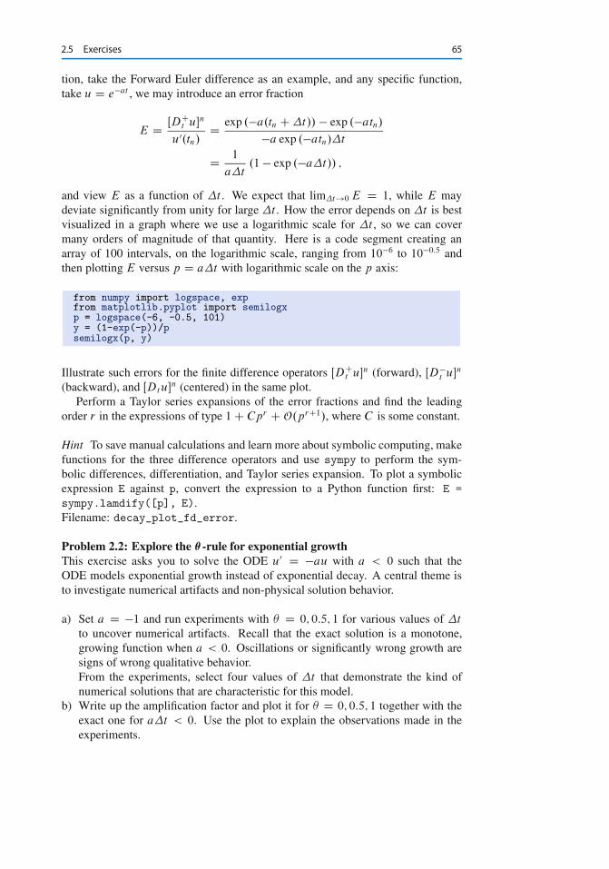
2.5 Exercises 65
tion, take the Forward Euler difference as an example, and any specific function,take u D e�at , we may introduce an error fraction
E D ŒDCt u�n
u0.tn/D exp .�a.tn C�t// � exp .�atn/
�a exp .�atn/�t
D 1
a�t.1 � exp .�a�t// ;
and view E as a function of �t . We expect that lim�t!0 E D 1, while E maydeviate significantly from unity for large �t . How the error depends on �t is bestvisualized in a graph where we use a logarithmic scale for �t , so we can covermany orders of magnitude of that quantity. Here is a code segment creating anarray of 100 intervals, on the logarithmic scale, ranging from 10�6 to 10�0:5 andthen plotting E versus p D a�t with logarithmic scale on the p axis:
from numpy import logspace, expfrom matplotlib.pyplot import semilogxp = logspace(-6, -0.5, 101)y = (1-exp(-p))/psemilogx(p, y)
Illustrate such errors for the finite difference operators ŒDCt u�n (forward), ŒD�t u�n
(backward), and ŒDtu�n (centered) in the same plot.Perform a Taylor series expansions of the error fractions and find the leading
order r in the expressions of type 1C Cpr CO.prC1/, where C is some constant.
Hint To save manual calculations and learn more about symbolic computing, makefunctions for the three difference operators and use sympy to perform the sym-bolic differences, differentiation, and Taylor series expansion. To plot a symbolicexpression E against p, convert the expression to a Python function first: E =sympy.lamdify([p], E).Filename: decay_plot_fd_error.
Problem 2.2: Explore the �-rule for exponential growthThis exercise asks you to solve the ODE u0 D �au with a < 0 such that theODE models exponential growth instead of exponential decay. A central theme isto investigate numerical artifacts and non-physical solution behavior.
a) Set a D �1 and run experiments with � D 0; 0:5; 1 for various values of �t
to uncover numerical artifacts. Recall that the exact solution is a monotone,growing function when a < 0. Oscillations or significantly wrong growth aresigns of wrong qualitative behavior.From the experiments, select four values of �t that demonstrate the kind ofnumerical solutions that are characteristic for this model.
b) Write up the amplification factor and plot it for � D 0; 0:5; 1 together with theexact one for a�t < 0. Use the plot to explain the observations made in theexperiments.
66 2 Analysis
Hint Modify the decay_ampf_plot.py6 code (in the src/analysis directory).Filename: exponential_growth.
Problem 2.3: Explore rounding errors in numerical calculus
a) Compute the absolute values of the errors in the numerical derivative of e�t
at t D 12
for three types of finite difference approximations: a forward differ-ence, a backward difference, and a centered difference, for �t D 2�k , k D0; 4; 8; 12; : : : ; 60. When do rounding errors destroy the accuracy?
b) Compute the absolute values of the errors in the numerical approximation ofR 4
0 e�t dt using the Trapezoidal and the Midpoint integration methods. Makea table of the errors for n D 2k intervals, k D 1; 3; 5; : : : ; 21. Is there anyimpact of rounding errors?
Hint The Trapezoidal rule forR b
af .x/dx reads
bZa
f .x/dx � h
1
2f .a/C 1
2f .b/C
n�1XiD1
f .aC ih/
!; h D b � a
n:
The Midpoint rule is
bZa
f .x/dx � h
nXiD1
f
�aC
�i C 1
2
�h
�:
Filename: rounding.
Open Access This chapter is distributed under the terms of the Creative Commons Attribution-NonCommercial 4.0 International License (http://creativecommons.org/licenses/by-nc/4.0/),which permits any noncommercial use, duplication, adaptation, distribution and reproductionin any medium or format, as long as you give appropriate credit to the original author(s) and thesource, a link is provided to the Creative Commons license and any changes made are indicated.
The images or other third party material in this chapter are included in the work’s CreativeCommons license, unless indicated otherwise in the credit line; if such material is not includedin the work’s Creative Commons license and the respective action is not permitted by statutoryregulation, users will need to obtain permission from the license holder to duplicate, adapt orreproduce the material.
6 http://tinyurl.com/ofkw6kc/analysis/decay_ampf_plot.py

3Generalizations
It is time to consider generalizations of the simple decay model u0 D �au and alsoto look at additional numerical solution methods. We consider first variable coeffi-cients, u0 D a.t/uC b.t/, and later a completely general scalar ODE u0 D f .u; t/
and its generalization to a system of such general ODEs. Among numerical meth-ods, we treat implicit multi-step methods, and several families of explicit methods:Leapfrog schemes, Runge–Kutta methods, and Adams–Bashforth formulas.
3.1 Model Extensions
This section looks at the generalizations to u0 D �a.t/u and u0 D �a.t/u Cb.t/. We sketch the corresponding implementations of the �-rule for such variable-coefficient ODEs. Verification can no longer make use of an exact solution of thenumerical problem so we make use of manufactured solutions, for deriving an exactsolution of the ODE problem, and then we can compute empirical convergence ratesfor the method and see if these coincide with the expected rates from theory. Finally,we see how our numerical methods can be applied to systems of ODEs.
The example programs associated with this chapter are found in the directorysrc/genz1.
3.1.1 Generalization: Including a Variable Coefficient
In the ODE for decay, u0 D �au, we now consider the case where a depends ontime:
u0.t/ D �a.t/u.t/; t 2 .0; T �; u.0/ D I : (3.1)
A Forward Euler scheme consists of evaluating (3.1) at t D tn and approximatingthe derivative with a forward difference ŒDCt u�n:
unC1 � un
�tD �a.tn/un : (3.2)
1 http://tinyurl.com/ofkw6kc/genz
67© The Author(s) 2016H.P. Langtangen, Finite Difference Computing with Exponential Decay Models,Lecture Notes in Computational Science and Engineering 110,DOI 10.1007/978-3-319-29439-1_3
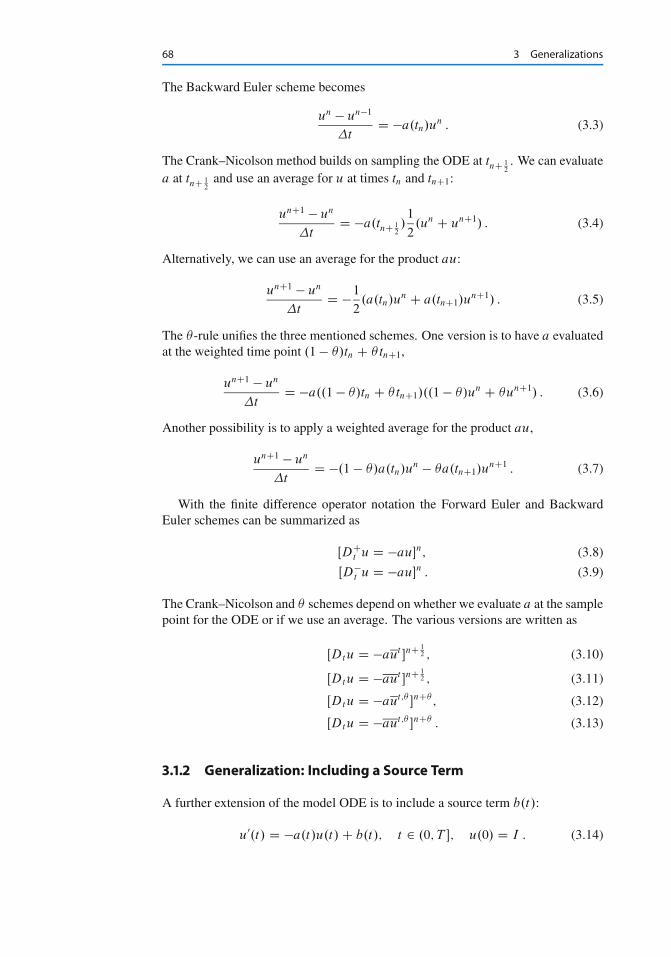
68 3 Generalizations
The Backward Euler scheme becomes
un � un�1
�tD �a.tn/un : (3.3)
The Crank–Nicolson method builds on sampling the ODE at tnC 12. We can evaluate
a at tnC 12
and use an average for u at times tn and tnC1:
unC1 � un
�tD �a.tnC 1
2/1
2.un C unC1/ : (3.4)
Alternatively, we can use an average for the product au:
unC1 � un
�tD �1
2.a.tn/un C a.tnC1/u
nC1/ : (3.5)
The �-rule unifies the three mentioned schemes. One version is to have a evaluatedat the weighted time point .1 � �/tn C � tnC1,
unC1 � un
�tD �a..1 � �/tn C � tnC1/..1 � �/un C �unC1/ : (3.6)
Another possibility is to apply a weighted average for the product au,
unC1 � un
�tD �.1 � �/a.tn/un � �a.tnC1/u
nC1 : (3.7)
With the finite difference operator notation the Forward Euler and BackwardEuler schemes can be summarized as
ŒDCt u D �au�n; (3.8)
ŒD�t u D �au�n : (3.9)
The Crank–Nicolson and � schemes depend on whether we evaluate a at the samplepoint for the ODE or if we use an average. The various versions are written as
ŒDtu D �aut �nC12 ; (3.10)
ŒDtu D �aut �nC12 ; (3.11)
ŒDtu D �aut;� �nC� ; (3.12)
ŒDtu D �aut;� �nC� : (3.13)
3.1.2 Generalization: Including a Source Term
A further extension of the model ODE is to include a source term b.t/:
u0.t/ D �a.t/u.t/C b.t/; t 2 .0; T �; u.0/ D I : (3.14)

3.1 Model Extensions 69
The time point where we sample the ODE determines where b.t/ is evaluated.For the Crank–Nicolson scheme and the �-rule we have a choice of whether toevaluate a.t/ and b.t/ at the correct point or use an average. The chosen strategybecomes particularly clear if we write up the schemes in the operator notation:
ŒDCt u D �auC b�n; (3.15)
ŒD�t u D �auC b�n; (3.16)
ŒDt u D �aut C b�nC12 ; (3.17)
ŒDt u D �auC bt�nC
12 ; (3.18)
ŒDt u D �aut;� C b�nC� ; (3.19)
ŒDt u D �auC bt;�
�nC� : (3.20)
3.1.3 Implementation of the Generalized Model Problem
Deriving the �-rule formula Writing out the �-rule in (3.20), using (1.44) and(1.45), we get
unC1 � un
�tD �.�anC1unC1 C bnC1//C .1 � �/.�anun C bn//; (3.21)
where an means evaluating a at t D tn and similar for anC1, bn, and bnC1. We solvefor unC1:
unC1 D ..1��t.1��/an/unC�t.�bnC1C.1��/bn//.1C�t�anC1/�1 : (3.22)
Python code Here is a suitable implementation of (3.21) where a.t/ and b.t/ aregiven as Python functions:
def solver(I, a, b, T, dt, theta):"""Solve u’=-a(t)*u + b(t), u(0)=I,for t in (0,T] with steps of dt.a and b are Python functions of t."""dt = float(dt) # avoid integer divisionNt = int(round(T/dt)) # no of time intervalsT = Nt*dt # adjust T to fit time step dtu = zeros(Nt+1) # array of u[n] valuest = linspace(0, T, Nt+1) # time mesh
u[0] = I # assign initial conditionfor n in range(0, Nt): # n=0,1,...,Nt-1
u[n+1] = ((1 - dt*(1-theta)*a(t[n]))*u[n] + \dt*(theta*b(t[n+1]) + (1-theta)*b(t[n])))/\(1 + dt*theta*a(t[n+1]))
return u, t
This function is found in the file decay_vc.py2 (vc stands for “variable coeffi-cients”).
2 http://tinyurl.com/ofkw6kc/genz/decay_vc.py

70 3 Generalizations
Coding of variable coefficients The solver function shown above demands thearguments a and b to be Python functions of time t, say
def a(t):return a_0 if t < tp else k*a_0
def b(t):return 1
Here, a(t) has three parameters a0, tp, and k, which must be global variables.A better implementation, which avoids global variables, is to represent a by
a class where the parameters are attributes and where a special method __call__evaluates a.t/:
class A:def __init__(self, a0=1, k=2):
self.a0, self.k = a0, k
def __call__(self, t):return self.a0 if t < self.tp else self.k*self.a0
a = A(a0=2, k=1) # a behaves as a function a(t)
For quick tests it is cumbersome to write a complete function or a class. Thelambda function construction in Python is then convenient. For example,
a = lambda t: a_0 if t < tp else k*a_0
is equivalent to the def a(t) definition above. In general,
f = lambda arg1, arg2, ...: expression
is equivalent to
def f(arg1, arg2, ...):return expression
One can use lambda functions directly in calls. Say we want to solve u0 D �uC 1,u.0/ D 2:
u, t = solver(2, lambda t: 1, lambda t: 1, T, dt, theta)
Whether to use a plain function, a class, or a lambda function depends on theprogrammer’s taste. Lazy programmers prefer the lambda construct, while verysafe programmers go for the class solution.
3.1.4 Verifying a Constant Solution
An extremely useful partial verification method is to construct a test problem witha very simple solution, usually u D const. Especially the initial debugging of

3.1 Model Extensions 71
a program code can benefit greatly from such tests, because 1) all relevant numericalmethods will exactly reproduce a constant solution, 2) many of the intermediatecalculations are easy to control by hand for a constant u, and 3) even a constant u
can uncover many bugs in an implementation.The only constant solution for the problem u0 D �au is u D 0, but too many
bugs can escape from that trivial solution. It is much better to search for a problemwhere u D C D const ¤ 0. Then u0 D �a.t/u C b.t/ is more appropriate: withu D C we can choose any a.t/ and set b D a.t/C and I D C . An appropriate testfunction is
def test_constant_solution():"""Test problem where u=u_const is the exact solution, to bereproduced (to machine precision) by any relevant method."""def u_exact(t):
return u_const
def a(t):return 2.5*(1+t**3) # can be arbitrary
def b(t):return a(t)*u_const
u_const = 2.15theta = 0.4; I = u_const; dt = 4Nt = 4 # enough with a few stepsu, t = solver(I=I, a=a, b=b, T=Nt*dt, dt=dt, theta=theta)print uu_e = u_exact(t)difference = abs(u_e - u).max() # max deviationtol = 1E-14assert difference < tol
An interesting question is what type of bugs that will make the computed un
deviate from the exact solution C . Fortunately, the updating formula and the initialcondition must be absolutely correct for the test to pass! Any attempt to makea wrong indexing in terms like a(t[n]) or any attempt to introduce an erroneousfactor in the formula creates a solution that is different from C .
3.1.5 Verification via Manufactured Solutions
Following the idea of the previous section, we can choose any formula as the exactsolution, insert the formula in the ODE problem and fit the data a.t/, b.t/, andI to make the chosen formula fulfill the equation. This powerful technique forgenerating exact solutions is very useful for verification purposes and known as themethod of manufactured solutions, often abbreviated MMS.
One common choice of solution is a linear function in the independent vari-able(s). The rationale behind such a simple variation is that almost any relevantnumerical solution method for differential equation problems is able to reproducea linear function exactly to machine precision (if u is about unity in size; precisionis lost if u takes on large values, see Exercise 3.1). The linear solution also makessome stronger demands to the numerical method and the implementation than the

72 3 Generalizations
constant solution used in Sect. 3.1.4, at least in more complicated applications.Still, the constant solution is often ideal for initial debugging before proceedingwith a linear solution.
We choose a linear solution u.t/ D ct C d . From the initial condition it followsthat d D I . Inserting this u in the left-hand side of (3.14), i.e., the ODE, we get
c D �a.t/uC b.t/ :
Any function u D ct C I is then a correct solution if we choose
b.t/ D c C a.t/.ct C I / :
With this b.t/ there are no restrictions on a.t/ and c.Let us prove that such a linear solution obeys the numerical schemes. To this
end, we must check that un D ca.tn/.ctn C I / fulfills the discrete equations. Forthese calculations, and later calculations involving linear solutions inserted in finitedifference schemes, it is convenient to compute the action of a difference operatoron a linear function t :
ŒDCt t �n D tnC1 � tn
�tD 1; (3.23)
ŒD�t t �n D tn � tn�1
�tD 1; (3.24)
ŒDt t�n D
tnC 12� tn� 1
2
�tD .nC 1
2/�t � .n � 1
2/�t
�tD 1 : (3.25)
Clearly, all three finite difference approximations to the derivative are exact foru.t/ D t or its mesh function counterpart un D tn.
The difference equation for the Forward Euler scheme
ŒDCt u D �auC b�n;
with an D a.tn/, bn D c C a.tn/.ctn C I /, and un D ctn C I then results in
c D �a.tn/.ctn C I /C c C a.tn/.ctn C I / D c
which is always fulfilled. Similar calculations can be done for the Backward Eulerand Crank–Nicolson schemes, or the �-rule for that matter. In all cases, un DctnC I is an exact solution of the discrete equations. That is why we should expectthat un � ue.tn/ D 0 mathematically and jun � ue.tn/j less than a small numberabout the machine precision for n D 0; : : : ; Nt .
The following function offers an implementation of this verification test basedon a linear exact solution:
def test_linear_solution():"""Test problem where u=c*t+I is the exact solution, to bereproduced (to machine precision) by any relevant method."""

3.1 Model Extensions 73
def u_exact(t):return c*t + I
def a(t):return t**0.5 # can be arbitrary
def b(t):return c + a(t)*u_exact(t)
theta = 0.4; I = 0.1; dt = 0.1; c = -0.5T = 4Nt = int(T/dt) # no of stepsu, t = solver(I=I, a=a, b=b, T=Nt*dt, dt=dt, theta=theta)u_e = u_exact(t)difference = abs(u_e - u).max() # max deviationprint differencetol = 1E-14 # depends on c!assert difference < tol
Any error in the updating formula makes this test fail!Choosing more complicated formulas as the exact solution, say cos.t/, will not
make the numerical and exact solution coincide to machine precision, because finitedifferencing of cos.t/ does not exactly yield the exact derivative � sin.t/. In suchcases, the verification procedure must be based on measuring the convergence ratesas exemplified in Sect. 3.1.6. Convergence rates can be computed as long as one hasan exact solution of a problem that the solver can be tested on, but this can alwaysbe obtained by the method of manufactured solutions.
3.1.6 Computing Convergence Rates
We expect that the error E in the numerical solution is reduced if the mesh size �t
is decreased. More specifically, many numerical methods obey a power-law relationbetween E and �t :
E D C�tr ; (3.26)
where C and r are (usually unknown) constants independent of �t . The formula(3.26) is viewed as an asymptotic model valid for sufficiently small �t . How smallis normally hard to estimate without doing numerical estimations of r .
The parameter r is known as the convergence rate. For example, if the conver-gence rate is 2, halving �t reduces the error by a factor of 4. Diminishing �t thenhas a greater impact on the error compared with methods that have r D 1. Fora given value of r , we refer to the method as of r-th order. First- and second-ordermethods are most common in scientific computing.
Estimating r There are two alternative ways of estimating C and r based on a setof m simulations with corresponding pairs .�ti ; Ei /, i D 0; : : : ; m � 1, and �ti <
�ti�1 (i.e., decreasing cell size).
1. Take the logarithm of (3.26), ln E D r ln �t C ln C , and fit a straight line to thedata points .�ti ; Ei /, i D 0; : : : ; m � 1.

74 3 Generalizations
2. Consider two consecutive experiments, .�ti ; Ei / and .�ti�1; Ei�1/. Dividingthe equation Ei�1 D C�tr
i�1 by Ei D C�tri and solving for r yields
ri�1 D ln.Ei�1=Ei /
ln.�ti�1=�ti /(3.27)
for i D 1; : : : ; m � 1. Note that we have introduced a subindex i � 1 on r
in (3.27) because r estimated from a pair of experiments must be expected tochange with i .
The disadvantage of method 1 is that (3.26) might not be valid for the coarsestmeshes (largest �t values). Fitting a line to all the data points is then misleading.Method 2 computes convergence rates for pairs of experiments and allows us to seeif the sequence ri converges to some value as i ! m � 2. The final rm�2 can thenbe taken as the convergence rate. If the coarsest meshes have a differing rate, thecorresponding time steps are probably too large for (3.26) to be valid. That is, thosetime steps lie outside the asymptotic range of �t values where the error behaveslike (3.26).
Implementation We can compute r0; r1; : : : ; rm�2 from Ei and �ti by the follow-ing function
def compute_rates(dt_values, E_values):m = len(dt_values)r = [log(E_values[i-1]/E_values[i])/
log(dt_values[i-1]/dt_values[i])for i in range(1, m, 1)]
# Round to two decimalsr = [round(r_, 2) for r_ in r]return r
Experiments with a series of time step values and � D 0; 1; 0:5 can be set up asfollows, here embedded in a real test function:
def test_convergence_rates():# Create a manufactured solution# define u_exact(t), a(t), b(t)
dt_values = [0.1*2**(-i) for i in range(7)]I = u_exact(0)
for theta in (0, 1, 0.5):E_values = []for dt in dt_values:
u, t = solver(I=I, a=a, b=b, T=6, dt=dt, theta=theta)u_e = u_exact(t)e = u_e - uE = sqrt(dt*sum(e**2))E_values.append(E)
r = compute_rates(dt_values, E_values)print ’theta=%g, r: %s’ % (theta, r)expected_rate = 2 if theta == 0.5 else 1tol = 0.1diff = abs(expected_rate - r[-1])assert diff < tol

3.1 Model Extensions 75
The manufactured solution is conveniently computed by sympy. Let us chooseue.t/ D sin.t/e�2t and a.t/ D t2. This implies that we must fit b as b.t/ Du0.t/ � a.t/. We first compute with sympy expressions and then we convert theexact solution, a, and b to Python functions that we can use in the subsequentnumerical computing:
# Create a manufactured solution with sympyimport sympy as symt = sym.symbols(’t’)u_e = sym.sin(t)*sym.exp(-2*t)a = t**2b = sym.diff(u_e, t) + a*u_exact
# Turn sympy expressions into Python functionu_exact = sym.lambdify([t], u_e, modules=’numpy’)a = sym.lambdify([t], a, modules=’numpy’)b = sym.lambdify([t], b, modules=’numpy’)
The complete code is found in the function test_convergence_rates in the filedecay_vc.py3.
Running this code gives the output
Terminal
theta=0, r: [1.06, 1.03, 1.01, 1.01, 1.0, 1.0]theta=1, r: [0.94, 0.97, 0.99, 0.99, 1.0, 1.0]theta=0.5, r: [2.0, 2.0, 2.0, 2.0, 2.0, 2.0]
We clearly see how the convergence rates approach the expected values.
Why convergence rates are importantThe strong practical application of computing convergence rates is for verifi-cation: wrong convergence rates point to errors in the code, and correct conver-gence rates bring strong support for a correct implementation. Experience showsthat bugs in the code easily destroy the expected convergence rate.
3.1.7 Extension to Systems of ODEs
Many ODE models involve more than one unknown function and more than oneequation. Here is an example of two unknown functions u.t/ and v.t/:
u0 D auC bv; (3.28)
v0 D cuC dv; (3.29)
for constants a; b; c; d . Applying the Forward Euler method to each equation resultsin a simple updating formula:
unC1 D un C�t.aun C bvn/; (3.30)
vnC1 D un C�t.cun C dvn/ : (3.31)
3 http://tinyurl.com/ofkw6kc/genz/decay_vc.py

76 3 Generalizations
On the other hand, the Crank–Nicolson or Backward Euler schemes result in a 22
linear system for the new unknowns. The latter scheme becomes
unC1 D un C�t.aunC1 C bvnC1/; (3.32)
vnC1 D vn C�t.cunC1 C dvnC1/ : (3.33)
Collecting unC1 as well as vnC1 on the left-hand side results in
.1 ��ta/unC1 C bvnC1 D un; (3.34)
cunC1 C .1 ��td/vnC1 D vn; (3.35)
which is a system of two coupled, linear, algebraic equations in two unknowns.These equations can be solved by hand (using standard techniques for two algebraicequations with two unknowns x and y), resulting in explicit formulas for unC1 andvnC1 that can be directly implemented. For systems of ODEs with many equationsand unknowns, one will express the coupled equations at each time level in matrixform and call software for numerical solution of linear systems of equations.
3.2 General First-Order ODEs
We now turn the attention to general, nonlinear ODEs and systems of such ODEs.Our focus is on numerical methods that can be readily reused for time-discretizationof PDEs, and diffusion PDEs in particular. The methods are just briefly listed,and we refer to the rich literature for more detailed descriptions and analysis – thebooks [2–4, 12] are all excellent resources on numerical methods for ODEs. Wealso demonstrate the Odespy Python interface to a range of different software forgeneral first-order ODE systems.
3.2.1 Generic Form of First-Order ODEs
ODEs are commonly written in the generic form
u0 D f .u; t/; u.0/ D I; (3.36)
where f .u; t/ is some prescribed function. As an example, our most general expo-nential decay model (3.14) has f .u; t/ D �a.t/u.t/C b.t/.
The unknown u in (3.36) may either be a scalar function of time t , or a vectorvalued function of t in case of a system of ODEs with m unknown components:
u.t/ D .u.0/.t/; u.1/.t/; : : : ; u.m�1/.t// :
In that case, the right-hand side is a vector-valued function with m components,
f .u; t/ D .f .0/.u.0/.t/; : : : ; u.m�1/.t//;
f .1/.u.0/.t/; : : : ; u.m�1/.t//;
:::
f .m�1/.u.0/.t/; : : : ; u.m�1/.t/// :
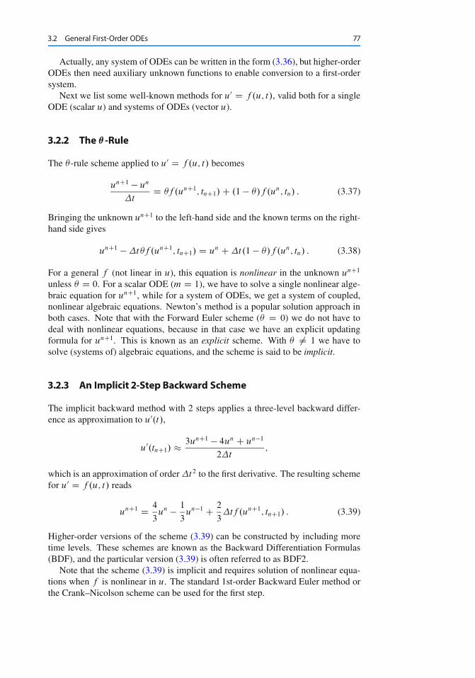
3.2 General First-Order ODEs 77
Actually, any system of ODEs can be written in the form (3.36), but higher-orderODEs then need auxiliary unknown functions to enable conversion to a first-ordersystem.
Next we list some well-known methods for u0 D f .u; t/, valid both for a singleODE (scalar u) and systems of ODEs (vector u).
3.2.2 The �-Rule
The �-rule scheme applied to u0 D f .u; t/ becomes
unC1 � un
�tD �f .unC1; tnC1/C .1 � �/f .un; tn/ : (3.37)
Bringing the unknown unC1 to the left-hand side and the known terms on the right-hand side gives
unC1 ��t�f .unC1; tnC1/ D un C�t.1 � �/f .un; tn/ : (3.38)
For a general f (not linear in u), this equation is nonlinear in the unknown unC1
unless � D 0. For a scalar ODE (m D 1), we have to solve a single nonlinear alge-braic equation for unC1, while for a system of ODEs, we get a system of coupled,nonlinear algebraic equations. Newton’s method is a popular solution approach inboth cases. Note that with the Forward Euler scheme (� D 0) we do not have todeal with nonlinear equations, because in that case we have an explicit updatingformula for unC1. This is known as an explicit scheme. With � ¤ 1 we have tosolve (systems of) algebraic equations, and the scheme is said to be implicit.
3.2.3 An Implicit 2-Step Backward Scheme
The implicit backward method with 2 steps applies a three-level backward differ-ence as approximation to u0.t/,
u0.tnC1/ � 3unC1 � 4un C un�1
2�t;
which is an approximation of order �t2 to the first derivative. The resulting schemefor u0 D f .u; t/ reads
unC1 D 4
3un � 1
3un�1 C 2
3�tf .unC1; tnC1/ : (3.39)
Higher-order versions of the scheme (3.39) can be constructed by including moretime levels. These schemes are known as the Backward Differentiation Formulas(BDF), and the particular version (3.39) is often referred to as BDF2.
Note that the scheme (3.39) is implicit and requires solution of nonlinear equa-tions when f is nonlinear in u. The standard 1st-order Backward Euler method orthe Crank–Nicolson scheme can be used for the first step.

78 3 Generalizations
3.2.4 Leapfrog Schemes
The ordinary Leapfrog scheme The derivative of u at some point tn can be ap-proximated by a central difference over two time steps,
u0.tn/ � unC1 � un�1
2�tD ŒD2tu�n (3.40)
which is an approximation of second order in �t . The scheme can then be writtenas
ŒD2t u D f .u; t/�n;
in operator notation. Solving for unC1 gives
unC1 D un�1 C 2�tf .un; tn/ : (3.41)
Observe that (3.41) is an explicit scheme, and that a nonlinear f (in u) is trivialto handle since it only involves the known un value. Some other scheme must beused as starter to compute u1, preferably the Forward Euler scheme since it is alsoexplicit.
The filtered Leapfrog scheme Unfortunately, the Leapfrog scheme (3.41) willdevelop growing oscillations with time (see Problem 3.6). A remedy for such unde-sired oscillations is to introduce a filtering technique. First, a standard Leapfrog stepis taken, according to (3.41), and then the previous un value is adjusted accordingto
un un C �.un�1 � 2un C unC1/ : (3.42)
The �-terms will effectively damp oscillations in the solution, especially those withshort wavelength (like point-to-point oscillations). A common choice of � is 0.6(a value used in the famous NCAR Climate Model).
3.2.5 The 2nd-Order Runge–Kutta Method
The two-step scheme
u� D un C�tf .un; tn/; (3.43)
unC1 D un C�t1
2.f .un; tn/C f .u�; tnC1// ; (3.44)
essentially applies a Crank–Nicolson method (3.44) to the ODE, but replaces theterm f .unC1; tnC1/ by a prediction f .u�; tnC1/ based on a Forward Euler step(3.43). The scheme (3.43)–(3.44) is known as Huen’s method, but is also a 2nd-order Runge–Kutta method. The scheme is explicit, and the error is expected tobehave as �t2.

3.2 General First-Order ODEs 79
3.2.6 A 2nd-Order Taylor-Series Method
One way to compute unC1 given un is to use a Taylor polynomial. We may write upa polynomial of 2nd degree:
unC1 D un C u0.tn/�t C 1
2u00.tn/�t2 :
From the equation u0 D f .u; t/ it follows that the derivatives of u can be expressedin terms of f and its derivatives:
u0.tn/ D f .un; tn/;
u00.tn/ D @f
@u.un; tn/u0.tn/C @f
@t
D f .un; tn/@f
@u.un; tn/C @f
@t;
resulting in the scheme
unC1 D un C f .un; tn/�t C 1
2
�f .un; tn/
@f
@u.un; tn/C @f
@t
��t2 : (3.45)
More terms in the series could be included in the Taylor polynomial to obtain meth-ods of higher order than 2.
3.2.7 The 2nd- and 3rd-Order Adams–Bashforth Schemes
The following method is known as the 2nd-order Adams–Bashforth scheme:
unC1 D un C 1
2�t�3f .un; tn/ � f .un�1; tn�1/
�: (3.46)
The scheme is explicit and requires another one-step scheme to compute u1 (theForward Euler scheme or Heun’s method, for instance). As the name implies, theerror behaves like �t2.
Another explicit scheme, involving four time levels, is the 3rd-order Adams–Bashforth scheme
unC1 D un C 1
12
�23f .un; tn/ � 16f .un�1; tn�1/C 5f .un�2; tn�2/
�: (3.47)
The numerical error is of order �t3, and the scheme needs some method for com-puting u1 and u2.
More general, higher-order Adams–Bashforth schemes (also called explicitAdams methods) compute unC1 as a linear combination of f at kC 1 previous timesteps:
unC1 D un CkX
jD0
j f .un�j ; tn�j /;
where j are known coefficients.

80 3 Generalizations
3.2.8 The 4th-Order Runge–Kutta Method
The perhaps most widely used method to solve ODEs is the 4th-order Runge–Kuttamethod, often called RK4. Its derivation is a nice illustration of common numericalapproximation strategies, so let us go through the steps in detail to learn aboutalgorithmic development.
The starting point is to integrate the ODE u0 D f .u; t/ from tn to tnC1:
u.tnC1/ � u.tn/ DtnC1Ztn
f .u.t/; t/dt :
We want to compute u.tnC1/ and regard u.tn/ as known. The task is to find good ap-proximations for the integral, since the integrand involves the unknown u betweentn and tnC1.
The integral can be approximated by the famous Simpson’s rule4:
tnC1Ztn
f .u.t/; t/dt � �t
6
�f n C 4f nC 1
2 C f nC1�
:
The problem now is that we do not know f nC 12 D f .unC 1
2 ; tnC 12/ and f nC1 D
.unC1; tnC1/ as we know only un and hence f n. The idea is to use various ap-proximations for f nC 1
2 and f nC1 based on well-known schemes for the ODE inthe intervals Œtn; tnC 1
2� and Œtn; tnC1�. We split the integral approximation into four
terms:tnC1Ztn
f .u.t/; t/dt � �t
6
�f n C 2 Of nC 1
2 C 2 Qf nC 12 C Nf nC1
�;
where Of nC 12 , Qf nC 1
2 , and Nf nC1 are approximations to f nC 12 and f nC1, respectively,
that can be based on already computed quantities. For Of nC 12 we can apply an ap-
proximation to unC 12 using the Forward Euler method with step 1
2�t :
Of nC 12 D f .un C 1
2�tf n; tnC 1
2/ (3.48)
Since this gives us a prediction of f nC 12 , we can for Qf nC 1
2 try a Backward Eulermethod to approximate unC 1
2 :
Qf nC 12 D f .un C 1
2�t Of nC 1
2 ; tnC 12/ : (3.49)
With Qf nC 12 as a hopefully good approximation to f nC 1
2 , we can for the final termNf nC1 use a Crank–Nicolson method on Œtn; tnC1� to approximate unC1:
Nf nC1 D f .un C�t Of nC 12 ; tnC1/ : (3.50)
4 http://en.wikipedia.org/wiki/Simpson’s_rule
3.2 General First-Order ODEs 81
We have now used the Forward and Backward Euler methods as well as the Crank–Nicolson method in the context of Simpson’s rule. The hope is that the combinationof these methods yields an overall time-stepping scheme from tn to tnC1 that ismuch more accurate than the O.�t/ and O.�t2/ of the individual steps. This isindeed true: the overall accuracy is O.�t4/!
To summarize, the 4th-order Runge–Kutta method becomes
unC1 D un C �t
6
�f n C 2 Of nC 1
2 C 2 Qf nC 12 C Nf nC1
�; (3.51)
where the quantities on the right-hand side are computed from (3.48)–(3.50). Notethat the scheme is fully explicit so there is never any need to solve linear or nonlinearalgebraic equations. However, the stability is conditional and depends on f . Thereis a whole range of implicit Runge–Kutta methods that are unconditionally stable,but require solution of algebraic equations involving f at each time step.
The simplest way to explore more sophisticated methods for ODEs is to applyone of the many high-quality software packages that exist, as the next section ex-plains.
3.2.9 The Odespy Software
A wide range of methods and software exist for solving (3.36). Many of the meth-ods are accessible through a unified Python interface offered by the Odespy5 [10]package. Odespy features simple Python implementations of the most fundamen-tal schemes as well as Python interfaces to several famous packages for solvingODEs: ODEPACK6, Vode7, rkc.f8, rkf45.f9, as well as the ODE solvers in SciPy10,SymPy11, and odelab12.
The code below illustrates the usage of Odespy the solving u0 D �au, u.0/ DI , t 2 .0; T �, by the famous 4th-order Runge–Kutta method, using �t D 1 andNt D 6 steps:
def f(u, t):return -a*u
import odespyimport numpy as np
I = 1; a = 0.5; Nt = 6; dt = 1solver = odespy.RK4(f)solver.set_initial_condition(I)t_mesh = np.linspace(0, Nt*dt, Nt+1)u, t = solver.solve(t_mesh)
5 https://github.com/hplgit/odespy6 https://computation.llnl.gov/casc/odepack/odepack_home.html7 https://computation.llnl.gov/casc/odepack/odepack_home.html8 http://www.netlib.org/ode/rkc.f9 http://www.netlib.org/ode/rkf45.f10 http://docs.scipy.org/doc/scipy/reference/generated/scipy.integrate.ode.html11 http://docs.sympy.org/dev/modules/mpmath/calculus/odes.html12 http://olivierverdier.github.com/odelab/

82 3 Generalizations
The previously listed methods for ODEs are all accessible in Odespy:
� the �-rule: ThetaRule� special cases of the �-rule: ForwardEuler, BackwardEuler,
CrankNicolson� the 2nd- and 4th-order Runge–Kutta methods: RK2 and RK4� The BDF methods and the Adam-Bashforth methods: Vode, Lsode, Lsoda,
lsoda_scipy� The Leapfrog schemes: Leapfrog and LeapfrogFiltered
3.2.10 Example: Runge–Kutta Methods
Since all solvers have the same interface in Odespy, except for a potentially differentset of parameters in the solvers’ constructors, one can easily make a list of solverobjects and run a loop for comparing a lot of solvers. The code below, found incomplete form in decay_odespy.py13, compares the famous Runge–Kutta meth-ods of orders 2, 3, and 4 with the exact solution of the decay equation u0 D �au.Since we have quite long time steps, we have included the only relevant �-rule forlarge time steps, the Backward Euler scheme (� D 1), as well. Figure 3.1 showsthe results.
import numpy as npimport matplotlib.pyplot as pltimport sys
def f(u, t):return -a*u
I = 1; a = 2; T = 6dt = float(sys.argv[1]) if len(sys.argv) >= 2 else 0.75Nt = int(round(T/dt))t = np.linspace(0, Nt*dt, Nt+1)
solvers = [odespy.RK2(f),odespy.RK3(f),odespy.RK4(f),]
# BackwardEuler must use Newton solver to converge# (Picard is default and leads to divergence)solvers.append(
odespy.BackwardEuler(f, nonlinear_solver=’Newton’))# Or tell BackwardEuler that it is a linear problemsolvers[-1] = odespy.BackwardEuler(f, f_is_linear=True,
jac=lambda u, t: -a)]legends = []for solver in solvers:
solver.set_initial_condition(I)u, t = solver.solve(t)
plt.plot(t, u)plt.hold(’on’)legends.append(solver.__class__.__name__)
13 http://tinyurl.com/ofkw6kc/genz/decay_odespy.py

3.2 General First-Order ODEs 83
Fig. 3.1 Behavior of different schemes for the decay equation
# Compare with exact solution plotted on a very fine mesht_fine = np.linspace(0, T, 10001)u_e = I*np.exp(-a*t_fine)plt.plot(t_fine, u_e, ’-’) # avoid markers by specifying line typelegends.append(’exact’)
plt.legend(legends)plt.title(’Time step: %g’ % dt)plt.show()
With the odespy.BackwardEuler method we must either tell that the problem islinear and provide the Jacobian of f .u; t/, i.e., @f=@u, as the jac argument, or wehave to assume that f is nonlinear, but then specify Newton’s method as solver forthe nonlinear equations (since the equations are linear, Newton’s method will con-verge in one iteration). By default, odespy.BackwardEuler assumes a nonlinearproblem to be solved by Picard iteration, but that leads to divergence in the presentproblem.
Visualization tipWe use Matplotlib for plotting here, but one could alternatively importscitools.std as plt instead. Plain use of Matplotlib as done here resultsin curves with different colors, which may be hard to distinguish on black-and-white paper. Using scitools.std, curves are automatically given colors and

84 3 Generalizations
markers, thus making curves easy to distinguish on screen with colors and onblack-and-white paper. The automatic adding of markers is normally a bad ideafor a very fine mesh since all the markers get cluttered, but scitools.stdlimits the number of markers in such cases. For the exact solution we use a veryfine mesh, but in the code above we specify the line type as a solid line (-),which means no markers and just a color to be automatically determined by thebackend used for plotting (Matplotlib by default, but scitools.std gives theopportunity to use other backends to produce the plot, e.g., Gnuplot or Grace).
Also note the that the legends are based on the class names of the solvers, andin Python the name of the class type (as a string) of an object obj is obtained byobj.__class__.__name__.
The runs in Fig. 3.1 and other experiments reveal that the 2nd-order Runge–Kuttamethod (RK2) is unstable for �t > 1 and decays slower than the Backward Eulerscheme for large and moderate �t (see Exercise 3.5 for an analysis). However, forfine �t D 0:25 the 2nd-order Runge–Kutta method approaches the exact solutionfaster than the Backward Euler scheme. That is, the latter scheme does a better jobfor larger �t , while the higher order scheme is superior for smaller �t . This isa typical trend also for most schemes for ordinary and partial differential equations.
The 3rd-order Runge–Kutta method (RK3) also has artifacts in the form of os-cillatory behavior for the larger �t values, much like that of the Crank–Nicolsonscheme. For finer �t , the 3rd-order Runge–Kutta method converges quickly to theexact solution.
The 4th-order Runge–Kutta method (RK4) is slightly inferior to the BackwardEuler scheme on the coarsest mesh, but is then clearly superior to all the otherschemes. It is definitely the method of choice for all the tested schemes.
Remark about using the �-rule in Odespy The Odespy package assumes thatthe ODE is written as u0 D f .u; t/ with an f that is possibly nonlinear in u. The�-rule for u0 D f .u; t/ leads to
unC1 D un C�t��f .unC1; tnC1/C .1 � �/f .un; tn/
�;
which is a nonlinear equation in unC1. Odespy’s implementation of the �-rule(ThetaRule) and the specialized Backward Euler (BackwardEuler) and Crank–Nicolson (CrankNicolson) schemes must invoke iterative methods for solving thenonlinear equation in unC1. This is done even when f is linear in u, as in themodel problem u0 D �au, where we can easily solve for unC1 by hand. There-fore, we need to specify use of Newton’s method to solve the equations. (Odespyallows other methods than Newton’s to be used, for instance Picard iteration, butthat method is not suitable. The reason is that it applies the Forward Euler schemeto generate a start value for the iterations. Forward Euler may give very wrong so-lutions for large �t values. Newton’s method, on the other hand, is insensitive tothe start value in linear problems.)

3.2 General First-Order ODEs 85
3.2.11 Example: Adaptive Runge–Kutta Methods
Odespy also offers solution methods that can adapt the size of �t with time to matcha desired accuracy in the solution. Intuitively, small time steps will be chosen inareas where the solution is changing rapidly, while larger time steps can be usedwhere the solution is slowly varying. Some kind of error estimator is used to adjustthe next time step at each time level.
A very popular adaptive method for solving ODEs is the Dormand-PrinceRunge–Kutta method of order 4 and 5. The 5th-order method is used as a referencesolution and the difference between the 4th- and 5th-order methods is used as anindicator of the error in the numerical solution. The Dormand-Prince method is thedefault choice in MATLAB’s widely used ode45 routine.
We can easily set up Odespy to use the Dormand-Prince method and see howit selects the optimal time steps. To this end, we request only one time step fromt D 0 to t D T and ask the method to compute the necessary non-uniform timemesh to meet a certain error tolerance. The code goes like
import odespyimport numpy as npimport decay_modimport sys#import matplotlib.pyplot as pltimport scitools.std as plt
def f(u, t):return -a*u
def u_exact(t):return I*np.exp(-a*t)
I = 1; a = 2; T = 5tol = float(sys.argv[1])solver = odespy.DormandPrince(f, atol=tol, rtol=0.1*tol)
Nt = 1 # just one step - let the scheme find# its intermediate points
t_mesh = np.linspace(0, T, Nt+1)t_fine = np.linspace(0, T, 10001)
solver.set_initial_condition(I)u, t = solver.solve(t_mesh)
# u and t will only consist of [I, u^Nt] and [0,T]# solver.u_all and solver.t_all contains all computed pointsplt.plot(solver.t_all, solver.u_all, ’ko’)plt.hold(’on’)plt.plot(t_fine, u_exact(t_fine), ’b-’)plt.legend([’tol=%.0E’ % tol, ’exact’])plt.savefig(’tmp_odespy_adaptive.png’)plt.show()
Running four cases with tolerances 10�1, 10�3, 10�5, and 10�7, gives the resultsin Fig. 3.2. Intuitively, one would expect denser points in the beginning of the decayand larger time steps when the solution flattens out.

86 3 Generalizations
Fig. 3.2 Choice of adaptive time mesh by the Dormand-Prince method for different tolerances
3.3 Exercises
Exercise 3.1: Experiment with precision in tests and the size of u
It is claimed in Sect. 3.1.5 that most numerical methods will reproduce a linearexact solution to machine precision. Test this assertion using the test functiontest_linear_solution in the decay_vc.py14 program. Vary the parameter cfrom very small, via c=1 to many larger values, and print out the maximum differ-ence between the numerical solution and the exact solution. What is the relevantvalue of the tolerance in the float comparison in each case?
Filename: test_precision.
Exercise 3.2: Implement the 2-step backward schemeImplement the 2-step backward method (3.39) for the model u0.t/ D �a.t/u.t/Cb.t/, u.0/ D I . Allow the first step to be computed by either the Backward Eulerscheme or the Crank–Nicolson scheme. Verify the implementation by choosinga.t/ and b.t/ such that the exact solution is linear in t (see Sect. 3.1.5). Showmathematically that a linear solution is indeed a solution of the discrete equations.
Compute convergence rates (see Sect. 3.1.6) in a test case using a D constand b D 0, where we easily have an exact solution, and determine if the choice
14 http://tinyurl.com/ofkw6kc/genz/decay_vc.py

3.3 Exercises 87
of a first-order scheme (Backward Euler) for the first step has any impact on theoverall accuracy of this scheme. The expected error goes like O.�t2/.
Filename: decay_backward2step.
Exercise 3.3: Implement the 2nd-order Adams–Bashforth schemeImplement the 2nd-order Adams–Bashforth method (3.46) for the decay problemu0 D �a.t/u C b.t/, u.0/ D I , t 2 .0; T �. Use the Forward Euler method forthe first step such that the overall scheme is explicit. Verify the implementationusing an exact solution that is linear in time. Analyze the scheme by searching forsolutions un D An when a D const and b D 0. Compare this second-order schemeto the Crank–Nicolson scheme.
Filename: decay_AdamsBashforth2.
Exercise 3.4: Implement the 3rd-order Adams–Bashforth schemeImplement the 3rd-order Adams–Bashforth method (3.47) for the decay problemu0 D �a.t/uC b.t/, u.0/ D I , t 2 .0; T �. Since the scheme is explicit, allow it tobe started by two steps with the Forward Euler method. Investigate experimentallythe case where b D 0 and a is a constant: Can we have oscillatory solutions forlarge �t?
Filename: decay_AdamsBashforth3.
Exercise 3.5: Analyze explicit 2nd-order methodsShow that the schemes (3.44) and (3.45) are identical in the case f .u; t/ D �a,where a > 0 is a constant. Assume that the numerical solution reads un D An forsome unknown amplification factor A to be determined. Find A and derive stabilitycriteria. Can the scheme produce oscillatory solutions of u0 D �au? Plot thenumerical and exact amplification factor.
Filename: decay_RK2_Taylor2.
Project 3.6: Implement and investigate the Leapfrog schemeA Leapfrog scheme for the ODE u0.t/ D �a.t/u.t/C b.t/ is defined by
ŒD2t u D �auC b�n : (3.52)
A separate method is needed to compute u1. The Forward Euler scheme is a possi-ble candidate.
a) Implement the Leapfrog scheme for the model equation. Plot the solution in thecase a D 1, b D 0, I D 1, �t D 0:01, t 2 Œ0; 4�. Compare with the exactsolution ue.t/ D e�t .
b) Show mathematically that a linear solution in t fulfills the Forward Euler schemefor the first step and the Leapfrog scheme for the subsequent steps. Use this lin-ear solution to verify the implementation, and automate the verification througha test function.
Hint It can be wise to automate the calculations such that it is easy to redo thecalculations for other types of solutions. Here is a possible sympy function that

88 3 Generalizations
takes a symbolic expression u (implemented as a Python function of t), fits the bterm, and checks if u fulfills the discrete equations:
import sympy as sym
def analyze(u):t, dt, a = sym.symbols(’t dt a’)
print ’Analyzing u_e(t)=%s’ % u(t)print ’u(0)=%s’ % u(t).subs(t, 0)
# Fit source term to the given u(t)b = sym.diff(u(t), t) + a*u(t)b = sym.simplify(b)print ’Source term b:’, b
# Residual in discrete equations; Forward Euler stepR_step1 = (u(t+dt) - u(t))/dt + a*u(t) - bR_step1 = sym.simplify(R_step1)print ’Residual Forward Euler step:’, R_step1
# Residual in discrete equations; Leapfrog stepsR = (u(t+dt) - u(t-dt))/(2*dt) + a*u(t) - bR = sym.simplify(R)print ’Residual Leapfrog steps:’, R
def u_e(t):return c*t + I
analyze(u_e)# or short form: analyze(lambda t: c*t + I)
c) Show that a second-order polynomial in t cannot be a solution of the discreteequations. However, if a Crank–Nicolson scheme is used for the first step,a second-order polynomial solves the equations exactly.
d) Create a manufactured solution u.t/ D sin.t/ for the ODE u0 D �au C b.Compute the convergence rate of the Leapfrog scheme using this manufacturedsolution. The expected convergence rate of the Leapfrog scheme is O.�t2/.Does the use of a 1st-order method for the first step impact the convergencerate?
e) Set up a set of experiments to demonstrate that the Leapfrog scheme (3.52) isassociated with numerical artifacts (instabilities). Document the main resultsfrom this investigation.
f) Analyze and explain the instabilities of the Leapfrog scheme (3.52):1. Choose a D const and b D 0. Assume that an exact solution of the discrete
equations has the form un D An, where A is an amplification factor to bedetermined. Derive an equation for A by inserting un D An in the Leapfrogscheme.
2. Compute A either by hand and/or with the aid of sympy. The polynomial forA has two roots, A1 and A2. Let un be a linear combination un D C1A
n1 C
C2An2 .
3. Show that one of the roots is the reason for instability.4. Compare A with the exact expression, using a Taylor series approximation.5. How can C1 and C2 be determined?
g) Since the original Leapfrog scheme is unconditionally unstable as time grows,it demands some stabilization. This can be done by filtering, where we first find

3.3 Exercises 89
unC1 from the original Leapfrog scheme and then replace un by un C �.un�1 �2un C unC1/, where � can be taken as 0.6. Implement the filtered Leapfrogscheme and check that it can handle tests where the original Leapfrog scheme isunstable.
Filename: decay_leapfrog.
Problem 3.7: Make a unified implementation of many schemesConsider the linear ODE problem u0.t/ D �a.t/u.t/ C b.t/, u.0/ D I . Explicitschemes for this problem can be written in the general form
unC1 DmX
jD0
cj un�j ; (3.53)
for some choice of c0; : : : ; cm. Find expressions for the cj coefficients in case ofthe �-rule, the three-level backward scheme, the Leapfrog scheme, the 2nd-orderRunge–Kutta method, and the 3rd-order Adams–Bashforth scheme.
Make a class ExpDecay that implements the general updating formula (3.53).The formula cannot be applied for n < m, and for those n values, other schemesmust be used. Assume for simplicity that we just repeat Crank–Nicolson steps until(3.53) can be used. Use a subclass to specify the list c0; : : : ; cm for a particularmethod, and implement subclasses for all the mentioned schemes. Verify the im-plementation by testing with a linear solution, which should be exactly reproducedby all methods.
Filename: decay_schemes_unified.
Open Access This chapter is distributed under the terms of the Creative Commons Attribution-NonCommercial 4.0 International License (http://creativecommons.org/licenses/by-nc/4.0/),which permits any noncommercial use, duplication, adaptation, distribution and reproductionin any medium or format, as long as you give appropriate credit to the original author(s) and thesource, a link is provided to the Creative Commons license and any changes made are indicated.
The images or other third party material in this chapter are included in the work’s CreativeCommons license, unless indicated otherwise in the credit line; if such material is not includedin the work’s Creative Commons license and the respective action is not permitted by statutoryregulation, users will need to obtain permission from the license holder to duplicate, adapt orreproduce the material.
4Models
This chapter presents many mathematical models that all end up with ODEs of thetype u0 D �auC b. The applications are taken from biology, finance, and physics,and cover population growth or decay, interacting predator-prey populations, com-pound interest and inflation, radioactive decay, chemical and biochemical reaction,spreading of diseases, cooling of objects, compaction of geological media, pressurevariations in the atmosphere, viscoelastic response in materials, and air resistanceon falling or rising bodies.
Before we turn to the applications, however, we take a brief look at the techniqueof scaling, which is so useful in many applications.
4.1 Scaling
Real applications of a model u0 D �auCb will often involve a lot of parameters inthe expressions for a and b. It can be quite a challenge to find relevant values of allparameters. In simple problems, however, it turns out that it is not always necessaryto estimate all parameters because we can lump them into one or a few dimension-less numbers by using a very attractive technique called scaling. It simply means tostretch the u and t axis in the present problem – and suddenly all parameters in theproblem are lumped into one parameter if b ¤ 0 and no parameter when b D 0!
4.1.1 Dimensionless Variables
Scaling means that we introduce a new function Nu.Nt /, with
Nu D u � um
uc
; Nt D t
tc;
where um is a characteristic value of u, uc is a characteristic size of the range ofu values, and tc is a characteristic size of the range of t where u shows signifi-cant variation. Choosing um, uc , and tc is not always easy and is often an art incomplicated problems. We just state one choice first:
uc D I; um D b=a; tc D 1=a :
91© The Author(s) 2016H.P. Langtangen, Finite Difference Computing with Exponential Decay Models,Lecture Notes in Computational Science and Engineering 110,DOI 10.1007/978-3-319-29439-1_4

92 4 Models
Inserting u D umCuc Nu and t D tc Nt in the problem u0 D �auCb, assuming a andb are constants, results (after some algebra) in the scaled problem
d Nud Nt D �Nu; Nu.0/ D 1 � ˇ;
where
ˇ D b
Ia:
4.1.2 Dimensionless Numbers
The parameter ˇ is a dimensionless number. From the equation we see that b musthave the same unit as the term au. The initial condition I must have the same unitas u, so Ia has the same unit as b, making the fraction b=.Ia/ dimensionless.
An important observation is that Nu depends on Nt and ˇ. That is, only the specialcombination of b=.Ia/ matters, not what the individual values of b, a, and I are.The original unscaled function u depends on t , b, a, and I .
A second observation is striking: if b D 0, the scaled problem is independent ofa and I ! In practice this means that we can perform a single numerical simulationof the scaled problem and recover the solution of any problem for a given a and I
by stretching the axis in the plot: u D I Nu and t D Nt=a. For b ¤ 0, we simulate thescaled problem for a few ˇ values and recover the physical solution u by translatingand stretching the u axis and stretching the t axis.
In general, scaling combines the parameters in a problem to a set of dimension-less parameters. The number of dimensionless parameters is usually much smallerthan the number of original parameters. Section 4.11 presents an example where 11parameters are reduced to one!
4.1.3 A Scaling for Vanishing Initial Condition
The scaling breaks down if I D 0. In that case we may choose um D 0, uc D b=a,and tc D 1=b, resulting in a slightly different scaled problem:
d Nud Nt D 1 � Nu; Nu.0/ D 0 :
As with b D 0, the case I D 0 has a scaled problem with no physical parameters!It is common to drop the bars after scaling and write the scaled problem as u0 D
�u, u.0/ D 1 � ˇ, or u0 D 1 � u, u.0/ D 0. Any implementation of the problemu0 D �auC b, u.0/ D I , can be reused for the scaled problem by setting a D 1,b D 0, and I D 1 � ˇ in the code, if I ¤ 0, or one sets a D 1, b D 1, and I D 0
when the physical I is zero. Falling bodies in fluids, as described in Sect. 4.11,involves u0 D �au C b with seven physical parameters. All these vanish in thescaled version of the problem if we start the motion from rest!
Many more details about scaling are presented in the author’s book Scaling ofDifferential Equations [9].

4.2 Evolution of a Population 93
4.2 Evolution of a Population
4.2.1 Exponential Growth
Let N be the number of individuals in a population occupying some spatial domain.Despite N being an integer in this problem, we shall compute with N as a real num-ber and view N.t/ as a continuous function of time. The basic model assumption isthat in a time interval �t the number of newcomers to the populations (newborns)is proportional to N , with proportionality constant Nb. The amount of newcomerswill increase the population and result in
N.t C�t/ D N.t/C NbN.t/ :
It is obvious that a long time interval �t will result in more newcomers and hencea larger Nb. Therefore, we introduce b D Nb=�t : the number of newcomers per unittime and per individual. We must then multiply b by the length of the time intervalconsidered and by the population size to get the total number of new individuals,b�tN .
If the number of removals from the population (deaths) is also proportional toN , with proportionality constant d�t , the population evolves according to
N.t C�t/ D N.t/C b�tN.t/ � d�tN.t/ :
Dividing by �t and letting �t ! 0, we get the ODE
N 0 D .b � d/N; N.0/ D N0 : (4.1)
In a population where the death rate (d ) is larger than then newborn rate (b), b�d <
0, and the population experiences exponential decay rather than exponential growth.In some populations there is an immigration of individuals into the spatial do-
main. With I individuals coming in per time unit, the equation for the populationchange becomes
N.t C�t/ D N.t/C b�tN.t/ � d�tN.t/C�tI :
The corresponding ODE reads
N 0 D .b � d/N C I; N.0/ D N0 : (4.2)
Emigration is also modeled by this I term if we just change its sign: I < 0. So, theI term models migration in and out of the domain in general.
Some simplification arises if we introduce a fractional measure of the population:u D N=N0 and set r D b � d . The ODE problem now becomes
u0 D ruC f; u.0/ D 1; (4.3)
where f D I=N0 measures the net immigration per time unit as the fraction ofthe initial population. Very often, r is approximately constant, but f is usuallya function of time.

94 4 Models
4.2.2 Logistic Growth
The growth rate r of a population decreases if the environment has limited re-sources. Suppose the environment can sustain at most Nmax individuals. We maythen assume that the growth rate approaches zero as N approaches Nmax, i.e., as u
approaches M D Nmax=N0. The simplest possible evolution of r is then a linearfunction: r.t/ D %.1�u.t/=M /, where % is the initial growth rate when the popula-tion is small relative to the maximum size and there is enough resources. Using thisr.t/ in (4.3) results in the logistic model for the evolution of a population (assumingfor the moment that f D 0):
u0 D %.1 � u=M /u; u.0/ D 1 : (4.4)
Initially, u will grow at rate %, but the growth will decay as u approaches M , andthen there is no more change in u, causing u!M as t !1. Note that the logisticequation u0 D %.1 � u=M /u is nonlinear because of the quadratic term �u2%=M .
4.3 Compound Interest and Inflation
Say the annual interest rate is r percent and that the bank adds the interest oncea year to your investment. If un is the investment in year n, the investment in yearunC1 grows to
unC1 D un C r
100un :
In reality, the interest rate is added every day. We therefore introduce a parameterm for the number of periods per year when the interest is added. If n counts theperiods, we have the fundamental model for compound interest:
unC1 D un C r
100mun : (4.5)
This model is a difference equation, but it can be transformed to a continuous dif-ferential equation through a limit process. The first step is to derive a formula forthe growth of the investment over a time t . Starting with an investment u0, andassuming that r is constant in time, we get
unC1 D�1C r
100m
�un
D�1C r
100m
�2
un�1
:::
D�1C r
100m
�nC1
u0
Introducing time t , which here is a real-numbered counter for years, we have thatn D mt , so we can write
umt D�1C r
100m
�mt
u0 :

4.4 Newton’s Law of Cooling 95
The second step is to assume continuous compounding, meaning that the interest isadded continuously. This implies m!1, and in the limit one gets the formula
u.t/ D u0ert=100; (4.6)
which is nothing but the solution of the ODE problem
u0 D r
100u; u.0/ D u0 : (4.7)
This is then taken as the ODE model for compound interest if r > 0. However,the reasoning applies equally well to inflation, which is just the case r < 0. Onemay also take the r in (4.7) as the net growth of an investment, where r takes bothcompound interest and inflation into account. Note that for real applications wemust use a time-dependent r in (4.7).
Introducing a D r100
, continuous inflation of an initial fortune I is then a processexhibiting exponential decay according to
u0 D �au; u.0/ D I :
4.4 Newton’s Law of Cooling
When a body at some temperature is placed in a cooling environment, experienceshows that the temperature falls rapidly in the beginning, and then the change intemperature levels off until the body’s temperature equals that of the surroundings.Newton carried out some experiments on cooling hot iron and found that the tem-perature evolved as a “geometric progression at times in arithmetic progression”,meaning that the temperature decayed exponentially. Later, this result was formu-lated as a differential equation: the rate of change of the temperature in a body isproportional to the temperature difference between the body and its surroundings.This statement is known as Newton’s law of cooling, which mathematically can beexpressed as
dT
dtD �k.T � Ts/; (4.8)
where T is the temperature of the body, Ts is the temperature of the surroundings(which may be time-dependent), t is time, and k is a positive constant. Equation(4.8) is primarily viewed as an empirical law, valid when heat is efficiently con-vected away from the surface of the body by a flowing fluid such as air at constanttemperature Ts . The heat transfer coefficient k reflects the transfer of heat from thebody to the surroundings and must be determined from physical experiments.
The cooling law (4.8) needs an initial condition T .0/ D T0.
4.5 Radioactive Decay
An atomic nucleus of an unstable atom may lose energy by emitting ionizing par-ticles and thereby be transformed to a nucleus with a different number of protonsand neutrons. This process is known as radioactive decay1. Actually, the process
1 http://en.wikipedia.org/wiki/Radioactive_decay
96 4 Models
is stochastic when viewed for a single atom, because it is impossible to predict ex-actly when a particular atom emits a particle. Nevertheless, with a large numberof atoms, N , one may view the process as deterministic and compute the meanbehavior of the decay. Below we reason intuitively about an ODE for the meanbehavior. Thereafter, we show mathematically that a detailed stochastic model forsingle atoms leads to the same mean behavior.
4.5.1 Deterministic Model
Suppose at time t , the number of the original atom type is N.t/. A basic modelassumption is that the transformation of the atoms of the original type in a smalltime interval �t is proportional to N , so that
N.t C�t/ D N.t/ � a�tN.t/;
where a > 0 is a constant. The proportionality factor is a�t , i.e., proportional to �t
since a longer time interval will produce more transformations. We can introduceu D N.t/=N.0/, divide by �t , and let �t ! 0:
limr!0
N0
u.t C�t/ � u.t/
�tD �aN0u.t/ :
The left-hand side is the derivative of u. Dividing by the N0 gives the followingODE for u:
u0 D �au; u.0/ D 1 : (4.9)
The parameter a can for a given nucleus be expressed through the half-life t1=2,which is the time taken for the decay to reduce the initial amount by one half, i.e.,u.t1=2/ D 0:5. With u.t/ D e�at , we get t1=2 D a�1 ln 2 or a D ln 2=t1=2.
4.5.2 Stochastic Model
Originally, we have N0 atoms. Up to some particular time t , each atom may eitherhave decayed or not. If not, they have “survived”. We want to count how many orig-inal atoms that have survived. The survival of a single atom at time t is a randomevent. Since there are only two outcomes, survival or decay, we have a Bernoullitrial2. Let p be the probability of survival (implying that the probability of decayis 1 � p). If each atom survives independently of the others, and the probability ofsurvival is the same for every atom, we have N0 Bernoulli trials, known as a bino-mial experiment from probability theory. The probability P.N / that N out of theN0 atoms have survived at time t is then given by the famous binomial distribution
P.N / D N0Š
N Š.N0 �N /ŠpN .1 � p/N0�N :
The mean (or expected) value EŒP � of P.N / is known to be N0p.
2 http://en.wikipedia.org/wiki/Bernoulli_trial

4.5 Radioactive Decay 97
It remains to estimate p. Let the interval Œ0; t � be divided into m small subinter-vals of length �t . We make the assumption that the probability of decay of a singleatom in an interval of length �t is Qp, and that this probability is proportional to �t :Qp D ��t (it sounds natural that the probability of decay increases with �t). The
corresponding probability of survival is 1 � ��t . Believing that � is independentof time, we have, for each interval of length �t , a Bernoulli trial: the atom eithersurvives or decays in that interval. Now, p should be the probability that the atomsurvives in all the intervals, i.e., that we have m successful Bernoulli trials in a rowand therefore
p D .1 � ��t/m :
The expected number of atoms of the original type at time t is
EŒP � D N0p D N0.1 � ��t/m; m D t=�t : (4.10)
To see the relation between the two types of Bernoulli trials and the ODE above,we go to the limit �t ! 0, m!1. It is possible to show that
p D limm!1.1 � ��t/m D lim
m!1
�1 � �
t
m
�m
D e��t
This is the famous exponential waiting time (or arrival time) distribution for a Pois-son process in probability theory (obtained here, as often done, as the limit ofa binomial experiment). The probability of decay, or more precisely that at leastone atom has undergone a transition, is 1 � p D 1 � e��t . This is the exponentialdistribution3. The limit means that m is very large, hence �t is very small, andQp D ��t is very small since the intensity of the events, �, is assumed finite. This
situation corresponds to a very small probability that an atom will decay in a veryshort time interval, which is a reasonable model. The same model occurs in lots ofdifferent applications, e.g., when waiting for a taxi, or when finding defects alonga rope.
4.5.3 Relation Between Stochastic and Deterministic Models
With p D e��t we get the expected number of original atoms at t as N0p D N0e��t ,
which is exactly the solution of the ODE model N 0 D ��N . This also gives aninterpretation of a via � or vice versa. Our important finding here is that the ODEmodel captures the mean behavior of the underlying stochastic model. This is,however, not always the common relation between microscopic stochastic modelsand macroscopic “averaged” models.
Also of interest, is that a Forward Euler discretization of N 0 D ��N , N.0/ DN0, gives N m D N0.1 � ��t/m at time tm D m�t , which is exactly the expectedvalue of the stochastic experiment with N0 atoms and m small intervals of length�t , where each atom can decay with probability ��t in an interval.
A fundamental question is how accurate the ODE model is. The underlyingstochastic model fluctuates around its expected value. A measure of the fluctuations
3 http://en.wikipedia.org/wiki/Exponential_distribution

98 4 Models
is the standard deviation of the binomial experiment with N0 atoms, which can beshown to be StdŒP � D pN0p.1 � p/. Compared to the size of the expectation, weget the normalized standard deviation
pVar.P /
EŒP �D N
�1=2
0
pp�1 � 1 D N
�1=2
0
q.1 � e��t /�1 � 1 � .N0�t/�1=2;
showing that the normalized fluctuations are very small if N0 is very large, whichis usually the case.
4.5.4 Generalization of the Radioactive Decay Modeling
The modeling in Sect. 4.5 is in fact very general, despite a focus on a particularphysical process. We may instead of atoms and decay speak about a set of items,where each item can undergo a stochastic transition from one state to another. InSect. 4.6 the item is a molecule and the transition is a chemical reaction, while inSect. 4.7 the item is an ill person and the transition is recovering from the illness (oran immune person who loses her immunity).
From the modeling in Sect. 4.5 we can establish a deterministic model for a largenumber of items and a stochastic model for an arbitrary number of items, evena single one. The stochastic model has a parameter � reflecting the probabilitythat a transition takes place in a time interval of unit length (or equivalently, thatthe probability is ��t for a transition during a time interval of length �t). Theprobability of making a transition before time t is given by
F.t/ D 1 � e��t :
The corresponding probability density is f .t/ D F 0.t/ D e��t . The expected valueof F.t/, i.e., the expected time to transition, is ��1. This interpretation of � makesit easy to measure its value: just carry out a large number of experiments, measurethe time to transition, and take one over the average of these times as an estimate of�. The variance is ��2.
The deterministic model counts how many items, N.t/, that have undergone thetransition (on average), and N.t/ is governed by the ODE
N 0 D ��N.t/; N.0/ D N0 :
4.6 Chemical Kinetics
4.6.1 Irreversible Reaction of Two Substances
Consider two chemical substances, A and B, and a chemical reaction that turns Ainto B. In a small time interval, some of the molecules of type A are transformedinto molecules of B. This process is, from a mathematical modeling point of view,equivalent to the radioactive decay process described in the previous section. We

4.6 Chemical Kinetics 99
can therefore apply the same modeling approach. If NA is the number of moleculesof substance A, we have that NA is governed by the differential equation
dNA
dtD �kNA;
where (the constant) k is called the rate constant of the reaction. Rather than us-ing the number of molecules, we use the concentration of molecules: ŒA�.t/ DNA.t/=NA.0/. We see that dŒA�=dt D NA.0/�1dNA=dt . Replacing NA by ŒA� inthe equation for NA leads to the equation for the concentration ŒA�:
dŒA�
dtD �kŒA�; t 2 .0; T �; ŒA�.0/ D 1 : (4.11)
Since substance A is transformed to substance B, we have that the concentration ofŒB� grows by the loss of ŒA�:
dŒB�
dtD kŒA�; ŒB�.0/ D 0 :
The mathematical model can either be (4.11) or the system
dŒA�
dtD �kŒA�; t 2 .0; T � (4.12)
dŒB�
dtD kŒA�; t 2 .0; T � (4.13)
ŒA�.0/ D 1; (4.14)
ŒB�.0/D 0 : (4.15)
This reaction is known as a first-order reaction, where each molecule of A makesan independent decision about whether to complete the reaction, i.e., independentof what happens to any other molecule.
An n-th order reaction is modeled by
dŒA�
dtD �kŒA�n; (4.16)
dŒB�
dtD kŒA�n; (4.17)
for t 2 .0; T � with initial conditions ŒA�.0/ D 1 and ŒB�.0/ D 0. Here, n can bea real number, but is most often an integer. Note that the sum of the concentrationsis constant since
dŒA�
dtC dŒB�
dtD 0 ) ŒA�.t/C ŒB�.t/ D const D ŒA�.0/C ŒB�.0/ D 1C 0 :
4.6.2 Reversible Reaction of Two Substances
Let the chemical reaction turn substance A into B and substance B into A. The rateof change of ŒA� has then two contributions: a loss kAŒA� and a gain kBŒB�:
dŒA�
dtD �kAŒA�C kBŒB�; t 2 .0; T �; ŒA�.0/ D A0 : (4.18)

100 4 Models
Similarly for substance B,
dŒB�
dtD kAŒA� � kBŒB�; t 2 .0; T �; ŒB�.0/ D B0 : (4.19)
This time we have allowed for arbitrary initial concentrations. Again,
dŒA�
dtC dŒB�
dtD 0 ) ŒA�.t/C ŒB�.t/ D A0 C B0 :
4.6.3 Irreversible Reaction of Two Substances into a Third
Now we consider two chemical substances, A and B, reacting with each other andproducing a substance C. In a small time interval �t , molecules of type A and Bare occasionally colliding, and in some of the collisions, a chemical reaction occurs,which turns A and B into a molecule of type C. (More generally, MA molecules of Aand MB molecules of B react to form MC molecules of C .) The number of possiblepairings, and thereby collisions, of A and B is NANB , where NA is the number ofmolecules of A, and NB is the number of molecules of B. A fraction k of thesecollisions, Ok�tNANB , features a chemical reaction and produce NC molecules ofC. The fraction is thought to be proportional to �t : considering a twice as long timeinterval, twice as many molecules collide, and twice as many reactions occur. Theincrease in molecules of substance C is now found from the reasoning
NC .t C�t/ D NC .t/C Ok�tNANB :
Dividing by �t ,NC .t C�t/ �NC .t/
�tD OkNANB;
and letting �t ! 0, gives the differential equation
dNC
dtD OkNANB :
(This equation is known as the important law of mass action4 discovered by theNorwegian scientists Cato M. Guldberg and Peter Waage. A more general form ofthe right-hand side is OkN ˛
A NˇB . All the constants Ok, ˛, and ˇ must be determined
from experiments.)Working instead with concentrations, we introduce ŒC �.t/ D NC .t/=NC .0/,
with similar definitions for ŒA� and ŒB� we get
dŒC �
dtD kŒA�ŒB� : (4.20)
4 https://en.wikipedia.org/wiki/Law_of_mass_action

4.7 Spreading of Diseases 101
The constant k is related to Ok by k D OkNA.0/NB.0/=NC .0/. The gain in C is a lossof A and B:
dŒA�
dtD �kŒA�ŒB�; (4.21)
dŒB�
dtD �kŒA�ŒB� : (4.22)
4.6.4 A Biochemical Reaction
A common reaction (known as Michaelis–Menten kinetics5) turns a substrate S intoa product P with aid of an enzyme E. The reaction is a two-stage process: first Sand E reacts to form a complex ES, where the enzyme and substrate are bound toeach other, and then ES is turned into E and P. In the first stage, S and E react toproduce a growth of ES according to the law of mass action:
dŒS�
dtD �kCŒE�ŒS�;
d ŒES�
dtD kCŒE�ŒS� :
The complex ES reacts and produces the product P at rate �kvŒES� and E at rate�k�ŒES�. The total set of reactions can then be expressed by
dŒES�
dtD kCŒE�ŒS�� kvŒES� � k�ŒES�; (4.23)
dŒP �
dtD kvŒES�; (4.24)
dŒS�
dtD �kCŒE�ŒS�C k�ŒES�; (4.25)
dŒE�
dtD �kCŒE�ŒS�C k�ŒES�C kvŒES� : (4.26)
The initial conditions are ŒES�.0/ D ŒP �.0/ D 0, and ŒS� D S0, ŒE� D E0. Theconstants kC, k�, and kv must be determined from experiments.
4.7 Spreading of Diseases
The modeling of spreading of diseases is very similar to the modeling of chemicalreactions in Sect. 4.6. The field of epidemiology speaks about susceptibles: peoplewho can get a disease; infectives: people who are infected and can infect suscep-tibles; and recovered: people who have recovered from the disease and becomeimmune. Three categories are accordingly defined: S for susceptibles, I for infec-tives, and R for recovered. The number in each category is tracked by the functionsS.t/, I.t/, and R.t/.
5 https://en.wikipedia.org/wiki/Michaelis-Menten_kinetics

102 4 Models
To model how many people that get infected in a small time interval �t , wereason as with reactions in Sect. 4.6. The possible number of pairings (“collisions”)between susceptibles and infected is SI . A fraction of these, ˇ�tSI , will actuallymeet and the infected succeed in infecting the susceptible, where ˇ is a parameter tobe empirically estimated. This leads to a loss of susceptibles and a gain of infected:
S.t C�t/ D S.t/ � ˇ�tSI;
I.t C�t/ D I.t/C ˇ�tSI :
In the same time interval, a fraction ��tI of the infected is recovered. It followsfrom Sect. 4.5.4 that the parameter ��1 is interpreted as the average waiting time toleave the I category, i.e., the average length of the disease. The ��tI term is a lossfor the I category, but a gain for the R category:
I.t C�t/ D I.t/C ˇ�tSI � ��tI; R.t C�t/ D R.t/C ��tI :
Dividing these equations by �t and going to the limit �t ! 0, gives the ODEsystem
dS
dtD �ˇSI; (4.27)
dI
dtD ˇSI � �I; (4.28)
dR
dtD �I; (4.29)
with initial values S.0/ D S0, I.0/ D I0, and R.0/ D 0. By adding the equations,we realize that
dS
dtC dI
dtC dR
dtD 0 ) S C I CR D const D N;
where N is the total number in the population under consideration. This propertycan be used as a partial verification during simulations.
Equations (4.27)–(4.29) are known as the SIR model in epidemiology. Themodel can easily be extended to incorporate vaccination programs, immunity lossafter some time, etc. Typical diseases that can be simulated by the SIR model andits variants are measles, smallpox, flu, plague, and HIV.
4.8 Predator-Prey Models in Ecology
A model for the interaction of predator and prey species can be based on reasoningfrom population dynamics and the SIR model. Let H.t/ be the number of preys ina region, and let L.t/ be the number of predators. For example, H may be haresand L lynx, or rabbits and foxes.
The population of the prey evolves due to births and deaths, exactly as in a pop-ulation dynamics model from Sect. 4.2.1. During a time interval �t the increase inthe population is therefore
H.t C�t/ �H.t/ D a�tH.t/;

4.9 Decay of Atmospheric Pressure with Altitude 103
where a is a parameter to be measured from data. The increase is proportional toH , and the proportionality constant a�t is proportional to �t , because doublingthe interval will double the increase.
However, the prey population has an additional loss because they are eaten bypredators. All the prey and predator animals can form LH pairs in total (assumingall individuals meet randomly). A small fraction b�t of such meetings, duringa time interval �t , ends up with the predator eating the prey. The increase in theprey population is therefore adjusted to
H.t C�t/ �H.t/ D a�tH.t/� b�tH.t/L.t/ :
The predator population increases as a result of eating preys. The amount ofeaten preys is b�tLH , but only a fraction d�tLH of this amount contributes toincreasing the predator population. In addition, predators die and this loss is set toc�tL. To summarize, the increase in the predator population is given by
L.t C�t/ � L.t/ D d�tL.t/H.t/ � c�tL.t/ :
Dividing by �t in the equations for H and L and letting t ! 0 results in
lim�t!0
H.t C�t/ �H.t/
�tD H 0.t/ D aH.t/ � bL.t/H.t/;
lim�t!0
L.t C�t/ �L.t/
�tD L0.t/ D dL.t/H.t/ � cL.t/ :
We can simplify the notation to the following two ODEs:
H 0 D H.a � bL/; (4.30)
L0 D L.dH � c/ : (4.31)
This is a so-called Lokta-Volterra model. It contains four parameters that must beestimated from data: a, b, c, and d . In addition, two initial conditions are neededfor H.0/ and L.0/.
4.9 Decay of Atmospheric Pressure with Altitude
4.9.1 The General Model
Vertical equilibrium of air in the atmosphere is governed by the equation
dp
dzD �%g : (4.32)
Here, p.z/ is the air pressure, % is the density of air, and g D 9:807 m=s2 is a stan-dard value of the acceleration of gravity. (Equation (4.32) follows directly from thegeneral Navier-Stokes equations for fluid motion, with the assumption that the airdoes not move.)

104 4 Models
The pressure is related to density and temperature through the ideal gas law
% D Mp
R�T; (4.33)
where M is the molar mass of the Earth’s air (0.029 kg=mol), R� is the universalgas constant (8:314 Nm/(mol K)), and T is the temperature in Kelvin. All variablesp, %, and T vary with the height z. Inserting (4.33) in (4.32) results in an ODE witha variable coefficient:
dp
dzD � Mg
R�T .z/p : (4.34)
4.9.2 Multiple Atmospheric Layers
The atmosphere can be approximately modeled by seven layers. In each layer,(4.34) is applied with a linear temperature of the form
T .z/ D NTi C Li.z � hi /;
where z D hi denotes the bottom of layer number i , having temperature NTi , and Li
is a constant in layer number i . The table below lists hi (m), NTi (K), and Li (K/m)for the layers i D 0; : : : ; 6.
i hiNTi Li
0 0 288 �0.00651 11,000 216 0.02 20,000 216 0.0013 32,000 228 0.00284 47,000 270 0.05 51,000 270 �0.00286 71,000 214 �0.002
For implementation it might be convenient to write (4.34) on the form
dp
dzD � Mg
R�. NT .z/C L.z/.z � h.z///p; (4.35)
where NT .z/, L.z/, and h.z/ are piecewise constant functions with values given inthe table. The value of the pressure at the sea level z D 0, p0 D p.0/, is 101,325 Pa.
4.9.3 Simplifications
Constant layer temperature One common simplification is to assume that thetemperature is constant within each layer. This means that L D 0.
One-layer model Another commonly used approximation is to work with onelayer instead of seven. This one-layer model6 is based on T .z/ D T0 � Lz,
6 http://en.wikipedia.org/wiki/Density_of_air

4.10 Compaction of Sediments 105
with sea level standard temperature T0 D 288 K and temperature lapse rate L D0:0065 K=m.
4.10 Compaction of Sediments
Sediments, originally made from materials like sand and mud, get compactedthrough geological time by the weight of new material that is deposited on the seabottom. The porosity � of the sediments tells how much void (fluid) space there isbetween the sand and mud grains. The porosity drops with depth, due to the weightof the sediments above. This makes the void space shrink, and thereby compactionincreases.
A typical assumption is that the change in � at some depth z is negatively pro-portional to �. This assumption leads to the differential equation problem
d�
dzD �c�; �.0/ D �0; (4.36)
where the z axis points downwards, z D 0 is the surface with known porosity, andc > 0 is a constant.
The upper part of the Earth’s crust consists of many geological layers stacked ontop of each other, as indicated in Fig. 4.1. The model (4.36) can be applied for eachlayer. In layer number i , we have the unknown porosity function �i .z/ fulfilling� 0i .z/ D �ci z, since the constant c in the model (4.36) depends on the type ofsediment in the layer. Alternatively, we can use (4.36) to describe the porositythrough all layers if c is taken as a piecewise constant function of z, equal to ci inlayer i . From the figure we see that new layers of sediments are deposited on topof older ones as time progresses. The compaction, as measured by �, is rapid in thebeginning and then decreases (exponentially) with depth in each layer.
When we drill a well at present time through the right-most column of sedimentsin Fig. 4.1, we can measure the thickness of the sediment in (say) the bottom layer.
Fig. 4.1 Illustration of the compaction of geological layers (with different colors) through time

106 4 Models
Let L1 be this thickness. Assuming that the volume of sediment remains constantthrough time, we have that the initial volume,
R L1;0
0�1dz, must equal the volume
seen today,R `
`�L1�1dz, where ` is the depth of the bottom of the sediment in the
present day configuration. After having solved for �1 as a function of z, we canthen find the original thickness L1;0 of the sediment from the equation
L1;0Z0
�1dz D`Z
`�L1
�1dz :
In hydrocarbon exploration it is important to know L1;0 and the compaction historyof the various layers of sediments.
4.11 Vertical Motion of a Body in a Viscous Fluid
A body moving vertically through a fluid (liquid or gas) is subject to three differenttypes of forces: the gravity force, the drag force7, and the buoyancy force.
4.11.1 Overview of Forces
Taking the upward direction as positive, the gravity force is Fg D �mg, where m
is the mass of the body and g is the acceleration of gravity. The uplift or buoyancyforce (“Archimedes force”) is Fb D %gV , where % is the density of the fluid and V
is the volume of the body.The drag force is of two types, depending on the Reynolds number
Re D %d jvj
; (4.37)
where d is the diameter of the body in the direction perpendicular to the flow, v
is the velocity of the body, and is the dynamic viscosity of the fluid. WhenRe < 1, the drag force is fairly well modeled by the so-called Stokes’ drag, whichfor a spherical body of diameter d reads
F.S/
d D �3dv : (4.38)
Quantities are taken as positive in the upwards vertical direction, so if v > 0 andthe body moves upwards, the drag force acts downwards and become negative, inaccordance with the minus sign in expression for F
.S/
d .For large Re, typically Re > 103, the drag force is quadratic in the velocity:
F.q/
d D �1
2CD%Ajvjv; (4.39)
7 http://en.wikipedia.org/wiki/Drag_(physics)

4.11 Vertical Motion of a Body in a Viscous Fluid 107
where CD is a dimensionless drag coefficient depending on the body’s shape, and A
is the cross-sectional area as produced by a cut plane, perpendicular to the motion,through the thickest part of the body. The superscripts q and S in F
.S/
d and F.q/
d
indicate Stokes’ drag and quadratic drag, respectively.
4.11.2 Equation ofMotion
All the mentioned forces act in the vertical direction. Newton’s second law of mo-tion applied to the body says that the sum of these forces must equal the mass of thebody times its acceleration a in the vertical direction.
ma D Fg C F.S/
d C Fb :
Here we have chosen to model the fluid resistance by the Stokes’ drag. Insertingthe expressions for the forces yields
ma D �mg � 3dvC %gV :
The unknowns here are v and a, i.e., we have two unknowns but only one equation.From kinematics in physics we know that the acceleration is the time derivative ofthe velocity: a D dv=dt . This is our second equation. We can easily eliminate a
and get a single differential equation for v:
mdv
dtD �mg � 3dvC %gV :
A small rewrite of this equation is handy: We express m as %bV , where %b is thedensity of the body, and we divide by the mass to get
v0.t/ D �3d
%bVv C g
�%
%b
� 1
�: (4.40)
We may introduce the constants
a D 3d
%bV; b D g
�%
%b
� 1
�; (4.41)
so that the structure of the differential equation becomes obvious:
v0.t/ D �av.t/C b : (4.42)
The corresponding initial condition is v.0/ D v0 for some prescribed starting ve-locity v0.
This derivation can be repeated with the quadratic drag force F.q/
d , leading to theresult
v0.t/ D �1
2CD
%A
%bVjvjv C g
�%
%b
� 1
�: (4.43)
108 4 Models
Defining
a D 1
2CD
%A
%bV; (4.44)
and b as above, we can write (4.43) as
v0.t/ D �ajvjv C b : (4.45)
4.11.3 Terminal Velocity
An interesting aspect of (4.42) and (4.45) is whether v will approach a final constantvalue, the so-called terminal velocity vT , as t ! 1. A constant v means thatv0.t/! 0 as t !1 and therefore the terminal velocity vT solves
0 D �avT C b
and0 D �ajvT jvT C b :
The former equation implies vT D b=a, while the latter has solutions vT D�pjbj=a for a falling body (vT < 0) and vT D
pb=a for a rising body (vT > 0).
4.11.4 A Crank–Nicolson Scheme
Both governing equations, the Stokes’ drag model (4.42) and the quadratic dragmodel (4.45), can be readily solved by the Forward Euler scheme. For higher ac-curacy one can use the Crank–Nicolson method, but a straightforward applicationof this method gives a nonlinear equation in the new unknown value vnC1 whenapplied to (4.45):
vnC1 � vn
�tD �a
1
2.jvnC1jvnC1 C jvnjvn/C b : (4.46)
The first term on the right-hand side of (4.46) is the arithmetic average of �jvjvevaluated at time levels n and nC 1.
Instead of approximating the term �jvjv by an arithmetic average, we can usea geometric mean:
.jvjv/nC 12 � jvnjvnC1 : (4.47)
The error is of second order in �t , just as for the arithmetic average and the centeredfinite difference approximation in (4.46). With the geometric mean, the resultingdiscrete equation
vnC1 � vn
�tD �ajvnjvnC1 C b

4.11 Vertical Motion of a Body in a Viscous Fluid 109
becomes a linear equation in vnC1, and we can therefore easily solve for vnC1:
vnC1 D vn C�tbnC 12
1C�tanC 12 jvnj
: (4.48)
Using a geometric mean instead of an arithmetic mean in the Crank–Nicolsonscheme is an attractive method for avoiding a nonlinear algebraic equation whendiscretizing a nonlinear ODE.
4.11.5 Physical Data
Suitable values of are 1:8 �10�5 Pa s for air and 8:9 �10�4 Pa s for water. Densitiescan be taken as 1:2 kg=m3 for air and as 1:0 � 103 kg=m3 for water. For consider-able vertical displacement in the atmosphere one should take into account that thedensity of air varies with the altitude, see Sect. 4.9. One possible density variationarises from the one-layer model in the mentioned section.
Any density variation makes b time dependent and we need bnC 12 in (4.48). To
compute the density that enters bnC 12 we must also compute the vertical position
z.t/ of the body. Since v D dz=dt , we can use a centered difference approxima-tion:
znC 12 � zn� 1
2
�tD vn ) znC 1
2 D zn� 12 C�t vn :
This znC 12 is used in the expression for b to compute %.znC 1
2 / and then bnC 12 .
The drag coefficient8 CD depends heavily on the shape of the body. Some valuesare: 0.45 for a sphere, 0.42 for a semi-sphere, 1.05 for a cube, 0.82 for a longcylinder (when the center axis is in the vertical direction), 0.75 for a rocket, 1.0-1.3for a man in upright position, 1.3 for a flat plate perpendicular to the flow, and 0.04for a streamlined, droplet-like body.
4.11.6 Verification
To verify the program, one may assume a heavy body in air such that the Fb forcecan be neglected, and further assume a small velocity such that the air resistance Fd
can also be neglected. This can be obtained by setting and % to zero. The motionthen leads to the velocity v.t/ D v0 � gt , which is linear in t and therefore shouldbe reproduced to machine precision (say tolerance 10�15) by any implementationbased on the Crank–Nicolson or Forward Euler schemes.
Another verification, but not as powerful as the one above, can be based oncomputing the terminal velocity and comparing with the exact expressions. Theadvantage of this verification is that we can also test the situation % ¤ 0.
As always, the method of manufactured solutions can be applied to test the im-plementation of all terms in the governing equation, but then the solution has nophysical relevance in general.
8 http://en.wikipedia.org/wiki/Drag_coefficient

110 4 Models
4.11.7 Scaling
Applying scaling, as described in Sect. 4.1, will for the linear case reduce the needto estimate values for seven parameters down to choosing one value of a singledimensionless parameter
ˇ D%bgV
�%
%b� 1
�3dI
;
provided I ¤ 0. If the motion starts from rest, I D 0, the scaled problem reads
Nu0 D 1 � Nu; Nu.0/ D 0;
and there is no need for estimating physical parameters (!). This means that thereis a single universal solution to the problem of a falling body starting from rest:Nu.t/ D 1 � e�Nt . All real physical cases correspond to stretching the Nt axis and theNu axis in this dimensionless solution. More precisely, the physical velocity u.t/ isrelated to the dimensionless velocity Nu.Nt/ through
u D%bgV
�%
%b� 1
�3d
Nu.t=.g.%=%b � 1/// D%bgV
�%
%b� 1
�3d
.1 � et=.g.%=%b�1/// :
4.12 Viscoelastic Materials
When stretching a rod made of a perfectly elastic material, the elongation (change inthe rod’s length) is proportional to the magnitude of the applied force. Mathematicalmodels for material behavior under application of external forces use strain " andstress � instead of elongation and forces. Strain is relative change in elongation andstress is force per unit area. An elastic material has a linear relation between stressand strain: � D E". This is a good model for many materials, but frequently thevelocity of the deformation (or more precisely, the strain rate "0) also influences thestress. This is particularly the case for materials like organic polymers, rubber, andwood. When the stress depends on both the strain and the strain rate, the materialis said to be viscoelastic. A common model relating forces to deformation is theKelvin–Voigt model9:
�.t/ D E".t/C �"0.t/ : (4.49)
Compared to a perfectly elastic material, which deforms instantaneously whena force is acting, a Kelvin–Voigt material will spend some time to elongate. Forexample, when an elastic rod is subject to a constant force � at t D 0, the strainimmediately adjusts to " D �=E. A Kelvin–Voigt material, however, has a response".t/ D �
E.1 � eEt=�/. Removing the force when the strain is ".t1/ D I will for
an elastic material immediately bring the strain back to zero, while a Kelvin–Voigtmaterial will decay: " D Ie�.t�t1/E=�/.
9 https://en.wikipedia.org/wiki/Kelvin-Voigt_material

4.13 Decay ODEs from Solving a PDE by Fourier Expansions 111
Introducing u for " and treating � .t/ as a given function, we can write theKelvin–Voigt model in our standard form
u0.t/ D �au.t/C b.t/; (4.50)
with a D E=� and b.t/ D � .t/=�. An initial condition, usually u.0/ D 0, isneeded.
4.13 Decay ODEs from Solving a PDE by Fourier Expansions
Suppose we have a partial differential equation
@u
@tD ˛
@2u
@x2C f .x; t/;
with boundary conditions u.0; t/ D u.L; t/ D 0 and initial condition u.x; 0/ DI.x/. One may express the solution as
u.x; t/ DmX
kD1
Ak.t/eikx=L;
for appropriate unknown functions Ak , k D 1; : : : ; m. We use the complex ex-ponential eikx=L for easy algebra, but the physical u is taken as the real part ofany complex expression. Note that the expansion in terms of eikx=L is compatiblewith the boundary conditions: all functions eikx=L vanish for x D 0 and x D L.Suppose we can express I.x/ as
I.x/ DmX
kD1
Ikeikx=L :
Such an expansion can be computed by well-known Fourier expansion techniques,but those details are not important here. Also, suppose we can express the givenf .x; t/ as
f .x; t/ DmX
kD1
bk.t/eikx=L :
Inserting the expansions for u and f in the differential equations demands that allterms corresponding to a given k must be equal. The calculations result in thefollow system of ODEs:
A0k.t/ D �˛k22
L2C bk.t/; k D 1; : : : ; m :
From the initial condition
u.x; 0/ DX
k
Ak.0/eikx=L D I.x/ DX
k
Ike.ikx=L/;

112 4 Models
so it follows that Ak.0/ D Ik , k D 1; : : : ; m. We then have m equations of theform A0k D �aAk C b, Ak.0/ D Ik , for appropriate definitions of a and b. TheseODE problems are independent of each other such that we can solve one problemat a time. The outlined technique is a quite common solution approach to partialdifferential equations.
Remark Since ak depends on k and the stability of the Forward Euler schemedemands ak�t � 1, we get that �t � ˛�1L2�2k�2 for this scheme. Usually, quitelarge k values are needed to accurately represent the given functions I and f so that�t in the Forward Euler scheme needs to be very small for these large values of k.Therefore, the Crank–Nicolson and Backward Euler schemes, which allow larger�t without any growth in the solutions, are more popular choices when creatingtime-stepping algorithms for partial differential equations of the type considered inthis example.
4.14 Exercises
Problem 4.1: Radioactive decay of Carbon-14The Carbon-1410 isotope, whose radioactive decay is used extensively in datingorganic material that is tens of thousands of years old, has a half-life of 5,730 years.Determine the age of an organic material that contains 8.4 % of its initial amount ofCarbon-14. Use a time unit of 1 year in the computations. The uncertainty in thehalf time of Carbon-14 is ˙40 years. What is the corresponding uncertainty in theestimate of the age?
Hint 1 Let A be the amount of Carbon-14. The ODE problem is then A0.t/ D�aA.t/, A.0/ D I . Introduced the scaled amount u D A=I . The ODE problemfor u is u0 D �au, u.0/ D 1. Measure time in years. Simulate until the first meshpoint tm such that u.tm/ � 0:084.
Hint 2 Use simulations with 5;730˙ 40 y as input and find the corresponding un-certainty interval for the result.Filename: carbon14.
Exercise 4.2: Derive schemes for Newton’s law of coolingShow in detail how we can apply the ideas of the Forward Euler, Backward Euler,and Crank–Nicolson discretizations to derive explicit computational formulas fornew temperature values in Newton’s law of cooling (see Sect. 4.4):
dT
dtD �k.T � Ts.t//; T .0/ D T0 :
Here, T is the temperature of the body, Ts.t/ is the temperature of the surroundings,t is time, k is the heat transfer coefficient, and T0 is the initial temperature of thebody. Summarize the discretizations in a �-rule such that you can get the threeschemes from a single formula by varying the � parameter.
Filename: schemes_cooling.
10 http://en.wikipedia.org/wiki/Carbon-14
4.14 Exercises 113
Exercise 4.3: Implement schemes for Newton’s law of coolingThe goal of this exercise is to implement the schemes from Exercise 4.2 and inves-tigate several approaches for verifying the implementation.
a) Implement the �-rule from Exercise 4.2 in a function
cooling(T0, k, T_s, t_end, dt, theta=0.5)
where T0 is the initial temperature, k is the heat transfer coefficient, T_s isa function of t for the temperature of the surroundings, t_end is the end time ofthe simulation, dt is the time step, and theta corresponds to � . The coolingfunction should return the temperature as an array T of values at the mesh pointsand the time mesh t.
b) In the case limt!1 Ts.t/ D C D const, explain why T .t/ ! C . Constructan example where you can illustrate this property in a plot. Implement a corre-sponding test function that checks the correctness of the asymptotic value of thesolution.
c) A piecewise constant surrounding temperature,
Ts.t/ D(
C0; 0 � t � t�
C1; t > t�;
corresponds to a sudden change in the environment at t D t�. Choose C0 D 2T0,C1 D 1
2T0, and t� D 3=k. Plot the solution T .t/ and explain why it seems
physically reasonable.d) We know from the ODE u0 D �au that the Crank–Nicolson scheme can give
non-physical oscillations for �t > 2=a. In the present problem, this resultsindicates that the Crank–Nicolson scheme give undesired oscillations for �t >
2=k. Discuss if this a potential problem in the physical case from c).e) Find an expression for the exact solution of T 0 D �k.T � Ts.t//, T .0/ D T0.
Construct a test case and compare the numerical and exact solution in a plot.Find a value of the time step �t such that the two solution curves cannot (vi-sually) be distinguished from each other. Many scientists will claim that sucha plot provides evidence for a correct implementation, but point out why therestill may be errors in the code. Can you introduce bugs in the cooling functionand still achieve visually coinciding curves?
Hint The exact solution can be derived by multiplying (4.8) by the integrating fac-tor ekt .
f) Implement a test function for checking that the solution returned by the coolingfunction is identical to the exact numerical solution of the problem (to machineprecision) when Ts is constant.
Hint The exact solution of the discrete equations in the case Ts is a constant canbe found by introducing u D T � Ts to get a problem u0 D �ku, u.0/ D T0 � Ts .The solution of the discrete equations is then of the form un D .T0 � Ts/A
n for

114 4 Models
some amplification factor A. The expression for T n is then T n D Ts.tn/ C un DTs C .T0 � Ts/A
n. We find that
A D 1 � .1 � �/k�t
1C �k�t:
The test function, testing several � values for a quite coarse mesh, may take theform
def test_discrete_solution():"""Compare the numerical solution with an exact solutionof the scheme when the T_s is constant."""T_s = 10T0 = 2k = 1.2dt = 0.1 # can use any meshN_t = 6 # any no of steps will dot_end = dt*N_tt = np.linspace(0, t_end, N_t+1)
for theta in [0, 0.5, 1, 0.2]:u, t = cooling(T0, k, lambda t: T_s , t_end, dt, theta)A = (1 - (1-theta)*k*dt)/(1 + theta*k*dt)u_discrete_exact = T_s + (T0-T_s)*A**(np.arange(len(t)))diff = np.abs(u - u_discrete_exact).max()print ’diff computed and exact discrete solution:’, difftol = 1E-14success = diff < tolassert success, ’diff=%g’ % diff
Running this function shows that the diff variable is 3.55E-15 as maximum soa tolerance of 10�14 is appropriate. This is a good test that the cooling functionworks!
Filename: cooling.
Exercise 4.4: Find time of murder from body temperatureA detective measures the temperature of a dead body to be 26.7 ıC at 2 pm. Onehour later the temperature is 25.8 ıC. The question is when death occurred.
Assume that Newton’s law of cooling (4.8) is an appropriate mathematical modelfor the evolution of the temperature in the body. First, determine k in (4.8) byformulating a Forward Euler approximation with one time steep from time 2 am totime 3 am, where knowing the two temperatures allows for finding k. Assume thetemperature in the air to be 20 ıC. Thereafter, simulate the temperature evolutionfrom the time of murder, taken as t D 0, when T D 37 ıC, until the temperaturereaches 25.8 ıC. The corresponding time allows for answering when death occurred.
Filename: detective.
Exercise 4.5: Simulate an oscillating cooling processThe surrounding temperature Ts in Newton’s law of cooling (4.8) may vary in time.Assume that the variations are periodic with period P and amplitude a around

4.14 Exercises 115
a constant mean temperature Tm:
Ts.t/ D Tm C a sin
�2
Pt
�: (4.51)
Simulate a process with the following data: k D 0:05 min�1, T .0/ D 5 ıC, Tm D25 ıC, a D 2:5 ıC, and P D 1 h, P D 10 min, and P D 6 h. Plot the T solutionsand Ts in the same plot.
Filename: osc_cooling.
Exercise 4.6: Simulate stochastic radioactive decayThe purpose of this exercise is to implement the stochastic model described inSect. 4.5 and show that its mean behavior approximates the solution of the cor-responding ODE model.
The simulation goes on for a time interval Œ0; T � divided into Nt intervals oflength �t . We start with N0 atoms. In some time interval, we have N atoms thathave survived. Simulate N Bernoulli trials with probability ��t in this intervalby drawing N random numbers, each being 0 (survival) or 1 (decay), where theprobability of getting 1 is ��t . We are interested in the number of decays, d , andthe number of survived atoms in the next interval is then N � d . The Bernoullitrials are simulated by drawing N uniformly distributed real numbers on Œ0; 1� andsaying that 1 corresponds to a value less than ��t :
# Given lambda_, dt, Nimport numpy as npuniform = np.random.uniform(N)Bernoulli_trials = np.asarray(uniform < lambda_*dt, dtype=np.int)d = Bernoulli_trials.size
Observe that uniform < lambda_*dt is a boolean array whose true and false val-ues become 1 and 0, respectively, when converted to an integer array.
Repeat the simulation over Œ0; T � a large number of times, compute the averagevalue of N in each interval, and compare with the solution of the correspondingODE model.
Filename: stochastic_decay.
Problem 4.7: Radioactive decay of two substancesConsider two radioactive substances A and B. The nuclei in substance A decay toform nuclei of type B with a half-life A1=2, while substance B decay to form typeA nuclei with a half-life B1=2. Letting uA and uB be the fractions of the initialamount of material in substance A and B, respectively, the following system ofODEs governs the evolution of uA.t/ and uB.t/:
1
ln 2u0A D uB=B1=2 � uA=A1=2; (4.52)
1
ln 2u0B D uA=A1=2 � uB=B1=2; (4.53)
with uA.0/ D uB.0/ D 1.

116 4 Models
a) Make a simulation program that solves for uA.t/ and uB.t/.b) Verify the implementation by computing analytically the limiting values of uA
and uB as t ! 1 (assume u0A; u0B ! 0) and comparing these with those ob-tained numerically.
c) Run the program for the case of A1=2 D 10 minutes and B1=2 D 50 minutes.Use a time unit of 1 minute. Plot uA and uB versus time in the same plot.
Filename: radioactive_decay_2subst.
Exercise 4.8: Simulate a simple chemical reactionConsider the simple chemical reaction where a substance A is turned into a sub-stance B according to
dŒA�
dtD �kŒA�;
d ŒB�
dtD kŒA�;
where ŒA� and ŒB� are the concentrations of A and B, respectively. It may be a chal-lenge to find appropriate values of k, but we can avoid this problem by workingwith a scaled model (as explained in Sect. 4.1). Scale the model above, using a timescale 1=k, and use the initial concentration of ŒA� as scale for ŒA� and ŒB�. Showthat the scaled system reads
du
dtD �u;
dv
dtD u;
with initial conditions u.0/ D 1, and v.0/ D ˛, where ˛ D ŒB�.0/=ŒA�.0/ isa dimensionless number, and u and v are the scaled concentrations of ŒA� and ŒB�,respectively. Implement a numerical scheme that can be used to find the solutionsu.t/ and v.t/. Visualize u and v in the same plot.
Filename: chemcial_kinetics_AB.
Exercise 4.9: Simulate an n-th order chemical reactionAn n-order chemical reaction, generalizing the model in Exercise 4.8, takes theform
dŒA�
dtD �kŒA�n;
d ŒB�
dtD kŒA�n;
where symbols are as defined in Exercise 4.8. Bring this model on dimensionlessform, using a time scale ŒA�.0/n�1=k, and show that the dimensionless model sim-

4.14 Exercises 117
plifies to
du
dtD �un;
dv
dtD un;
with u.0/ D 1 and v.0/ D ˛ D ŒB�.0/=ŒA�.0/. Solve numerically for u.t/ andshow a plot with u for n D 0:5; 1; 2; 4.
Filename: chemcial_kinetics_ABn.
Exercise 4.10: Simulate a biochemical processThe purpose of this exercise is to simulate the ODE system (4.23)–(4.26) modelinga simple biochemical process.
a) Scale (4.23)–(4.26) such that we can work with dimensionless parameters,which are easier to prescribe. Introduce
NQ D ŒES�
Qc
; NP D P
Pc
; NS D S
S0
; NE D E
E0
; Nt D t
tc;
where appropriate scales are
Qc D S0E0
K; Pc D Qc; tc D 1
kCE0
;
with K D .kv C k�/=kC (Michaelis constant). Show that the scaled systembecomes
d NQd Nt D ˛. NE NS � NQ/; (4.54)
d NPd Nt D ˇ NQ; (4.55)
d NSd Nt D �
NE NS C .1 � ˇ˛�1/ NQ; (4.56)
d NEd Nt D �
NE NS C NQ; (4.57)
where we have three dimensionless parameters
˛ D K
E0
; ˇ D kv
kCE0
; D E0
S0
:
The corresponding initial conditions are NQ D NP D 0 and NS D NE D 1.b) Implement a function for solving (4.54)–(4.57).c) There are two conservation equations implied by (4.23)–(4.26):
ŒES�C ŒE� D E0; (4.58)
ŒES�C ŒS�C ŒP � D S0 : (4.59)

118 4 Models
Derive these two equations. Use these properties in the function in b) to doa partial verification of the solution at each time step.
d) Simulate a case with T D 8, ˛ D 1:5 and ˇ D 1, and two values: 0.9 and 0.1.
Filename: biochem.
Exercise 4.11: Simulate spreading of a diseaseThe SIR model (4.27)–(4.29) can be used to simulate spreading of an epidemicdisease.
a) Estimating the parameter ˇ is difficult so it can be handy to scale the equations.Use tc D 1=� as time scale, and scale S , I , and R by the population sizeN D S.0/CI.0/CR.0/. Show that the resulting dimensionless model becomes
d NSd Nt D �R0
NS NI ; (4.60)
d NId Nt D R0
NS NI � NI ; (4.61)
d NRd Nt D I; (4.62)
NS.0/ D 1 � ˛; (4.63)
NI .0/ D ˛; (4.64)
NR.0/ D 0; (4.65)
where R0 and ˛ are the only parameters in the problem:
R0 D Nˇ
�; ˛ D I.0/
N:
A quantity with a bar denotes a dimensionless version of that quantity, e.g, Nt isdimensionless time, and Nt D �t .
b) Show that the R0 parameter governs whether the disease will spread or not att D 0.
Hint Spreading means dI=dt > 0.
c) Implement the scaled SIR model. Check at every time step, as a verification,that NS C NI C NR D 1.
d) Simulate the spreading of a disease where R0 D 2; 5 and 2 % of the populationis infected at time t D 0.
Filename: SIR.
Exercise 4.12: Simulate predator-prey interactionSection 4.8 describes a model for the interaction of predator and prey populations,such as lynx and hares.

4.14 Exercises 119
a) Scale the equations (4.30)–(4.31). Use the initial population H.0/ D H0 of H
has scale for H and L, and let the time scale be 1=.bH0/.b) Implement the scaled model from a). Run illustrating cases how the two popu-
lations develop.c) The scaling in a) used a scale for H and L based on the initial condition H.0/ D
H0. An alternative scaling is to make the ODEs as simple as possible by intro-ducing separate scales Hc and Lc for H and L, respectively. Fit Hc , Lc , andthe time scale tc such that there are as few dimensionless parameters as possi-ble in the ODEs. Scale the initial conditions. Compare the number and type ofdimensionless parameters with a).
d) Compute with the scaled model from c) and create plots to illustrate the typicalsolutions.
Filename: predator_prey.
Exercise 4.13: Simulate the pressure drop in the atmosphereWe consider the models for atmospheric pressure in Sect. 4.9. Make a program withthree functions,
� one computing the pressure p.z/ using a seven-layer model and varying L,� one computing p.z/ using a seven-layer model, but with constant temperature in
each layer, and� one computing p.z/ based on the one-layer model.
How can these implementations be verified? Should ease of verification impact howyou code the functions? Compare the three models in a plot.
Filename: atmospheric_pressure.
Exercise 4.14: Make a program for vertical motion in a fluidImplement the Stokes’ drag model (4.40) and the quadratic drag model (4.43) fromSect. 4.11, using the Crank–Nicolson scheme and a geometric mean for jvjv asexplained, and assume constant fluid density. At each time level, compute theReynolds number Re and choose the Stokes’ drag model if Re < 1 and the quadraticdrag model otherwise.
The computation of the numerical solution should take place either in a stand-alone function or in a solver class that looks up a problem class for physical data.Create a module and equip it with pytest/nose compatible test functions for auto-matically verifying the code.
Verification tests can be based on
� the terminal velocity (see Sect. 4.11),� the exact solution when the drag force is neglected (see Sect. 4.11),� the method of manufactured solutions (see Sect. 3.1.5) combined with comput-
ing convergence rates (see Sect. 3.1.6).
Use, e.g., a quadratic polynomial for the velocity in the method of manufacturedsolutions. The expected error is O.�t2/ from the centered finite difference approx-imation and the geometric mean approximation for jvjv.

120 4 Models
A solution that is linear in t will also be an exact solution of the discrete equa-tions in many problems. Show that this is true for linear drag (by adding a sourceterm that depends on t), but not for quadratic drag because of the geometric meanapproximation. Use the method of manufactured solutions to add a source term inthe discrete equations for quadratic drag such that a linear function of t is a so-lution. Add a test function for checking that the linear function is reproduced tomachine precision in the case of both linear and quadratic drag.
Apply the software to a case where a ball rises in water. The buoyancy force ishere the driving force, but the drag will be significant and balance the other forcesafter a short time. A soccer ball has radius 11 cm and mass 0.43 kg. Start the motionfrom rest, set the density of water, %, to 1000 kg=m3, set the dynamic viscosity, ,to 10�3 Pa s, and use a drag coefficient for a sphere: 0.45. Plot the velocity of therising ball.
Filename: vertical_motion.
Project 4.15: Simulate parachutingThe aim of this project is to develop a general solver for the vertical motion ofa body with quadratic air drag, verify the solver, apply the solver to a skydiver infree fall, and finally apply the solver to a complete parachute jump.
All the pieces of software implemented in this project should be realized asPython functions and/or classes and collected in one module.
a) Set up the differential equation problem that governs the velocity of the motion.The parachute jumper is subject to the gravity force and a quadratic drag force.Assume constant density. Add an extra source term to be used for programverification. Identify the input data to the problem.
b) Make a Python module for computing the velocity of the motion. Also equipthe module with functionality for plotting the velocity.
Hint 1 Use the Crank–Nicolson scheme with a geometric mean of jvjv in time tolinearize the equation of motion with quadratic drag.
Hint 2 You can either use functions or classes for implementation. If you choosefunctions, make a function solver that takes all the input data in the problem asarguments and that returns the velocity (as a mesh function) and the time mesh. Incase of a class-based implementation, introduce a problem class with the physicaldata and a solver class with the numerical data and a solve method that stores thevelocity and the mesh in the class.
Allow for a time-dependent area and drag coefficient in the formula for the dragforce.
c) Show that a linear function of t does not fulfill the discrete equations because ofthe geometric mean approximation used for the quadratic drag term. Fit a sourceterm, as in the method of manufactured solutions, such that a linear function oft is a solution of the discrete equations. Make a test function to check that thissolution is reproduced to machine precision.

4.14 Exercises 121
d) The expected error in this problem goes like �t2 because we use a centered finitedifference approximation with error O.�t2/ and a geometric mean approxima-tion with error O.�t2/. Use the method of manufactured solutions combinedwith computing convergence rate to verify the code. Make a test function forchecking that the convergence rate is correct.
e) Compute the drag force, the gravity force, and the buoyancy force as a functionof time. Create a plot with these three forces.
Hint You can either make a function forces(v, t, plot=None) that returns theforces (as mesh functions) and t, and shows a plot on the screen and also savesthe plot to a file with name stored in plot if plot is not None, or you can extendthe solver class with computation of forces and include plotting of forces in thevisualization class.
f) Compute the velocity of a skydiver in free fall before the parachute opens.
Hint Meade and Struthers [11] provide some data relevant to skydiving11. Themass of the human body and equipment can be set to 100 kg. A skydiver in spread-eagle formation has a cross-section of 0.5 m2 in the horizontal plane. The densityof air decreases with altitude, but can be taken as constant, 1 kg=m3, for altitudesrelevant to skydiving (0–4000 m). The drag coefficient for a man in upright positioncan be set to 1.2. Start with a zero velocity. A free fall typically has a terminatingvelocity of 45 m=s. (This value can be used to tune other parameters.)
g) The next task is to simulate a parachute jumper during free fall and after theparachute opens. At time tp , the parachute opens and the drag coefficient and thecross-sectional area change dramatically. Use the program to simulate a jumpfrom z D 3000 m to the ground z D 0. What is the maximum acceleration,measured in units of g, experienced by the jumper?
Hint Following Meade and Struthers [11], one can set the cross-section area per-pendicular to the motion to 44 m2 when the parachute is open. Assume that it takes8 s to increase the area linearly from the original to the final value. The drag coeffi-cient for an open parachute can be taken as 1.8, but tuned using the known value ofthe typical terminating velocity reached before landing: 5.3 m=s. One can take thedrag coefficient as a piecewise constant function with an abrupt change at tp . Theparachute is typically released after tp D 60 s, but larger values of tp can be used tomake plots more illustrative.Filename: parachuting.
Exercise 4.16: Formulate vertical motion in the atmosphereVertical motion of a body in the atmosphere needs to take into account a varying airdensity if the range of altitudes is many kilometers. In this case, % varies with thealtitude z. The equation of motion for the body is given in Sect. 4.11. Let us assumequadratic drag force (otherwise the body has to be very, very small). A differential
11 http://en.wikipedia.org/wiki/Parachuting

122 4 Models
equation problem for the air density, based on the information for the one-layeratmospheric model in Sect. 4.9, can be set up as
p0.z/ D � Mg
R�.T0 C Lz/p; (4.66)
% D pM
R�T: (4.67)
To evaluate p.z/ we need the altitude z. From the principle that the velocity is thederivative of the position we have that
z0.t/ D v.t/; (4.68)
where v is the velocity of the body.Explain in detail how the governing equations can be discretized by the Forward
Euler and the Crank–Nicolson methods. Discuss pros and cons of the two methods.Filename: falling_in_variable_density.
Exercise 4.17: Simulate vertical motion in the atmosphereImplement the Forward Euler or the Crank–Nicolson scheme derived in Exer-cise 4.16. Demonstrate the effect of air density variation on a falling human, e.g.,the famous fall of Felix Baumgartner12. The drag coefficient can be set to 1.2.
Filename: falling_in_variable_density.
Problem 4.18: Compute y D jxj by solving an ODEConsider the ODE problem
y0.x/ D(�1; x < 0;
1; x 0x 2 .�1; 1�; y.1�/ D 1;
which has the solution y.x/ D jxj. Using a mesh x0 D �1, x1 D 0, andx2 D 1, calculate by hand y1 and y2 from the Forward Euler, Backward Euler,Crank–Nicolson, and Leapfrog methods. Use all of the former three methods forcomputing the y1 value to be used in the Leapfrog calculation of y2. Thereafter, vi-sualize how these schemes perform for a uniformly partitioned mesh with N D 10
and N D 11 points.Filename: signum.
Problem 4.19: Simulate fortune growth with random interest rateThe goal of this exercise is to compute the value of a fortune subject to inflation anda random interest rate. Suppose that the inflation is constant at i percent per yearand that the annual interest rate, p, changes randomly at each time step, starting atsome value p0 at t D 0. The random change is from a value pn at t D tn to pnC�p
with probability 0.25 and pn � �p with probability 0.25. No change occurs withprobability 0.5. There is also no change if pnC1 exceeds 15 or becomes below 1.Use a time step of one month, p0 D i , initial fortune scaled to 1, and simulate 1000
12 http://en.wikipedia.org/wiki/Felix_Baumgartner

4.14 Exercises 123
scenarios of length 20 years. Compute the mean evolution of one unit of moneyand the corresponding standard deviation. Plot the mean curve along with the meanplus one standard deviation and the mean minus one standard deviation. This willillustrate the uncertainty in the mean curve.
Hint 1 The following code snippet computes pnC1:
import random
def new_interest_rate(p_n, dp=0.5):r = random.random() # uniformly distr. random number in [0,1)if 0 <= r < 0.25:
p_np1 = p_n + dpelif 0.25 <= r < 0.5:
p_np1 = p_n - dpelse:
p_np1 = p_nreturn (p_np1 if 1 <= p_np1 <= 15 else p_n)
Hint 2 If ui .t/ is the value of the fortune in experiment number i , i D 0; : : : ; N�1,the mean evolution of the fortune is
Nu.t/ D 1
N
N�1XiD0
ui .t/;
and the standard deviation is
s.t/ Dvuut 1
N � 1
�. Nu.t//2 C
N�1XiD0
.ui .t//2
!:
Suppose ui .t/ is stored in an array u. The mean and the standard deviation ofthe fortune is most efficiently computed by using two accumulation arrays, sum_uand sum_u2, and performing sum_u += u and sum_u2 += u**2 after every ex-periment. This technique avoids storing all the ui .t/ time series for computing thestatistics.Filename: random_interest.
Exercise 4.20: Simulate a population in a changing environmentWe shall study a population modeled by (4.3) where the environment, representedby r and f , undergoes changes with time.
a) Assume that there is a sudden drop (increase) in the birth (death) rate at timet D tr , because of limited nutrition or food supply:
r.t/ D(
%; t < tr ;
% �A; t tr :
This drop in population growth is compensated by a sudden net immigration attime tf > tr :
f .t/ D(
0; t < tf ;
f0; t ta:

124 4 Models
Start with % and make A > %. Experiment with these and other parameters toillustrate the interplay of growth and decay in such a problem.
b) Now we assume that the environmental conditions changes periodically withtime so that we may take
r.t/ D %C A sin�
2
Pt
�:
That is, the combined birth and death rate oscillates around % with a maximumchange of ˙A repeating over a period of length P in time. Set f D 0 andexperiment with the other parameters to illustrate typical features of the solution.
Filename: population.py.
Exercise 4.21: Simulate logistic growthSolve the logistic ODE (4.4) using a Crank–Nicolson scheme where .unC 1
2 /2 isapproximated by a geometric mean:
.unC 12 /2 � unC1un :
This trick makes the discrete equation linear in unC1.Filename: logistic_CN.
Exercise 4.22: Rederive the equation for continuous compound interestThe ODE model (4.7) was derived under the assumption that r was constant. Per-form an alternative derivation without this assumption: 1) start with (4.5); 2) intro-duce a time step �t instead of m: �t D 1=m if t is measured in years; 3) divide by�t and take the limit �t ! 0. Simulate a case where the inflation is at a constantlevel I percent per year and the interest rate oscillates: r D �I=2 C r0 sin.2t/.Compare solutions for r0 D I; 3I=2; 2I .
Filename: interest_modeling.
Exercise 4.23: Simulate the deformation of a viscoelastic materialStretching a rod made of polymer will cause deformations that are well describedwith a Kelvin–Voigt material model (4.49). At t D 0 we apply a constant force� D �0, but at t D t1, we remove the force so � D 0. Compute numerically thecorresponding strain (elongation divided by the rod’s length) and visualize how itresponds in time.
Hint To avoid finding proper values of the E and � parameters for a polymer, onecan scale the problem. A common dimensionless time is Nt D tE=�. Note that " isalready dimensionless by definition, but it takes on small values, say up to 0.1, sowe introduce a scaling: Nu D 10" such that Nu takes on values up to about unity.
Show that the material model then takes the form Nu0 D � NuC 10�.t/=E. Workwith the dimensionless force F D 10�.t/=E, and let F D 1 for Nt 2 .0; Nt1/ andF D 0 for Nt Nt1. A possible choice of t1 is the characteristic time �=E, whichmeans that Nt1 D 1.Filename: KelvinVoigt.

4.14 Exercises 125
Open Access This chapter is distributed under the terms of the Creative Commons Attribution-NonCommercial 4.0 International License (http://creativecommons.org/licenses/by-nc/4.0/),which permits any noncommercial use, duplication, adaptation, distribution and reproductionin any medium or format, as long as you give appropriate credit to the original author(s) and thesource, a link is provided to the Creative Commons license and any changes made are indicated.
The images or other third party material in this chapter are included in the work’s CreativeCommons license, unless indicated otherwise in the credit line; if such material is not includedin the work’s Creative Commons license and the respective action is not permitted by statutoryregulation, users will need to obtain permission from the license holder to duplicate, adapt orreproduce the material.

5Scientific Software Engineering
Teaching material on scientific computing has traditionally been very focused onthe mathematics and the applications, while details on how the computer is pro-grammed to solve the problems have received little attention. Many end up writingas simple programs as possible, without being aware of much useful computer sci-ence technology that would increase the fun, efficiency, and reliability of the theirscientific computing activities.
This chapter demonstrates a series of good practices and tools from modern com-puter science, using the simple mathematical problem u0 D �au, u.0/ D I , suchthat we minimize the mathematical details and can go more in depth with implemen-tations. The goal is to increase the technological quality of computer programmingand make it match the more well-established quality of the mathematics of scientificcomputing.
The conventions and techniques outlined here will save you a lot of time whenyou incrementally extend software over time from simpler to more complicatedproblems. In particular, you will benefit from many good habits:
� new code is added in a modular fashion to a library (modules),� programs are run through convenient user interfaces,� it takes one quick command to let all your code undergo heavy testing,� tedious manual work with running programs is automated,� your scientific investigations are reproducible,� scientific reports with top quality typesetting are produced both for paper and
electronic devices.
5.1 Implementations with Functions andModules
All previous examples in this book have implemented numerical algorithms asPython functions. This is a good style that readers are expected to adopt. How-ever, this author has experienced that many students and engineers are inclined tomake “flat” programs, i.e., a sequence of statements without any use of functions,just to get the problem solved as quickly as possible. Since this programming styleis so widespread, especially among people with MATLAB experience, we shall
127© The Author(s) 2016H.P. Langtangen, Finite Difference Computing with Exponential Decay Models,Lecture Notes in Computational Science and Engineering 110,DOI 10.1007/978-3-319-29439-1_5

128 5 Scientific Software Engineering
look at the weaknesses of flat programs and show how they can be refactored intomore reusable programs based on functions.
5.1.1 Mathematical Problem and Solution Technique
We address the differential equation problem
u0.t/ D �au.t/; t 2 .0; T �; (5.1)
u.0/ D I; (5.2)
where a, I , and T are prescribed parameters, and u.t/ is the unknown function tobe estimated. This mathematical model is relevant for physical phenomena featur-ing exponential decay in time, e.g., vertical pressure variation in the atmosphere,cooling of an object, and radioactive decay.
As we learned in Chap. 1.1.2, the time domain is discretized with points 0 Dt0 < t1 � � � < tNt
D T , here with a constant spacing �t between the mesh points:�t D tn � tn�1, n D 1; : : : ; Nt . Let un be the numerical approximation to theexact solution at tn. A family of popular numerical methods are provided by the �
scheme,
unC1 D 1 � .1 � �/a�t
1C �a�tun; (5.3)
for n D 0; 1; : : : ; Nt � 1. This formula produces the Forward Euler scheme when� D 0, the Backward Euler scheme when � D 1, and the Crank–Nicolson schemewhen � D 1=2.
5.1.2 A First, Quick Implementation
Solving (5.3) in a program is very straightforward: just make a loop over n andevaluate the formula. The u.tn/ values for discrete n can be stored in an array. Thismakes it easy to also plot the solution. It would be natural to also add the exactsolution curve u.t/ D Ie�at to the plot.
Many have programming habits that would lead them to write a simple programlike this:
from numpy import *from matplotlib.pyplot import *
A = 1a = 2T = 4dt = 0.2N = int(round(T/dt))y = zeros(N+1)t = linspace(0, T, N+1)theta = 1y[0] = Afor n in range(0, N):
y[n+1] = (1 - (1-theta)*a*dt)/(1 + theta*dt*a)*y[n]

5.1 Implementations with Functions and Modules 129
y_e = A*exp(-a*t) - yerror = y_e - yE = sqrt(dt*sum(error**2))print ’Norm of the error: %.3E’ % Eplot(t, y, ’r--o’)t_e = linspace(0, T, 1001)y_e = A*exp(-a*t_e)plot(t_e, y_e, ’b-’)legend([’numerical, theta=%g’ % theta, ’exact’])xlabel(’t’)ylabel(’y’)show()
This program is easy to read, and as long as it is correct, many will claim that ithas sufficient quality. Nevertheless, the program suffers from two serious flaws:
1. The notation in the program does not correspond exactly to the notation in themathematical problem: the solution is called y and corresponds to u in the math-ematical description, the variable A corresponds to the mathematical parameterI , N in the program is called Nt in the mathematics.
2. There are no comments in the program.
These kind of flaws quickly become crucial if present in code for complicated math-ematical problems and code that is meant to be extended to other problems.
We also note that the program is flat in the sense that it does not contain func-tions. Usually, this is a bad habit, but let us first correct the two mentioned flaws.
5.1.3 AMore Decent Program
A code of better quality arises from fixing the notation and adding comments:
from numpy import *from matplotlib.pyplot import *
I = 1a = 2T = 4dt = 0.2Nt = int(round(T/dt)) # no of time intervalsu = zeros(Nt+1) # array of u[n] valuest = linspace(0, T, Nt+1) # time meshtheta = 1 # Backward Euler method
u[0] = I # assign initial conditionfor n in range(0, Nt): # n=0,1,...,Nt-1
u[n+1] = (1 - (1-theta)*a*dt)/(1 + theta*dt*a)*u[n]
# Compute norm of the erroru_e = I*exp(-a*t) - u # exact u at the mesh pointserror = u_e - uE = sqrt(dt*sum(error**2))print ’Norm of the error: %.3E’ % E
# Compare numerical (u) and exact solution (u_e) in a plotplot(t, u, ’r--o’)t_e = linspace(0, T, 1001) # very fine mesh for u_eu_e = I*exp(-a*t_e)

130 5 Scientific Software Engineering
plot(t_e, u_e, ’b-’)legend([’numerical, theta=%g’ % theta, ’exact’])xlabel(’t’)ylabel(’u’)show()
Comments in a program There is obviously not just one way to comment a pro-gram, and opinions may differ as to what code should be commented. The guidingprinciple is, however, that comments should make the program easy to understandfor the human eye. Do not comment obvious constructions, but focus on ideas and(“what happens in the next statements?”) and on explaining code that can be foundcomplicated.
Refactoring into functions At first sight, our updated program seems like a goodstarting point for playing around with the mathematical problem: we can justchange parameters and rerun. Although such edit-and-rerun sessions are good forinitial exploration, one will soon extend the experiments and start developing thecode further. Say we want to compare � D 0; 1; 0:5 in the same plot. This extensionrequires changes all over the code and quickly leads to errors. To do somethingserious with this program, we have to break it into smaller pieces and make sureeach piece is well tested, and ensure that the program is sufficiently general and canbe reused in new contexts without changes. The next natural step is therefore toisolate the numerical computations and the visualization in separate Python func-tions. Such a rewrite of a code, without essentially changing the functionality, butjust improve the quality of the code, is known as refactoring. After quickly puttingtogether and testing a program, the next step is to refactor it so it becomes betterprepared for extensions.
Program file vs IDE vs notebook There are basically three different ways ofworking with Python code:
1. One writes the code in a file, using a text editor (such as Emacs or Vim) andruns it in a terminal window.
2. One applies an Integrated Development Environment (the simplest is IDLE,which comes with standard Python) containing a graphical user interface withan editor and an element where Python code can be run.
3. One applies the Jupyter Notebook (previously known as IPython Notebook),which offers an interactive environment for Python code where plots are auto-matically inserted after the code, see Fig. 5.1.
It appears that method 1 and 2 are quite equivalent, but the notebook encouragesmore experimental code and therefore also flat programs. Consequently, notebookusers will normally need to think more about refactoring code and increase the useof functions after initial experimentation.

5.1 Implementations with Functions and Modules 131
Fig. 5.1 Experimental code in a notebook
5.1.4 Prefixing Imported Functions by theModule Name
Import statements of the form from module import * import all functions andvariables in module.py into the current file. This is often referred to as “importstar”, and many find this convenient, but it is not considered as a good programmingstyle in Python. For example, when doing
from numpy import *from matplotlib.pyplot import *
we get mathematical functions like sin and exp as well as MATLAB-style func-tions like linspace and plot, which can be called by these well-known names.Unfortunately, it sometimes becomes confusing to know where a particular func-tion comes from, i.e., what modules you need to import. Is a desired function fromnumpy or matplotlib.pyplot? Or is it our own function? These questions areeasy to answer if functions in modules are prefixed by the module name. Doing anadditional from math import * is really crucial: now sin, cos, and other mathe-matical functions are imported and their names hide those previously imported fromnumpy. That is, sin is now a sine function that accepts a float argument, not anarray.

132 5 Scientific Software Engineering
Doing the import such that module functions must have a prefix is generallyrecommended:
import numpyimport matplotlib.pyplot
t = numpy.linspace(0, T, Nt+1)u_e = I*numpy.exp(-a*t)matplotlib.pyplot.plot(t, u_e)
The modules numpy and matplotlib.pyplot are frequently used, and sincetheir full names are quite tedious to write, two standard abbreviations have evolvedin the Python scientific computing community:
import numpy as npimport matplotlib.pyplot as plt
t = np.linspace(0, T, Nt+1)u_e = I*np.exp(-a*t)plt.plot(t, u_e)
The downside of prefixing functions by the module name is that mathematicalexpressions like e�at sin.2t/ get cluttered with module names,
numpy.exp(-a*t)*numpy.sin(2(numpy.pi*t)# ornp.exp(-a*t)*np.sin(2*np.pi*t)
Such an expression looks like exp(-a*t)*sin(2*pi*t) in most other program-ming languages. Similarly, np.linspace and plt.plot look less familiar topeople who are used to MATLAB and who have not adopted Python’s prefix style.Whether to do from module import * or import module depends on personaltaste and the problem at hand. In these writings we use from module import *in more basic, shorter programs where similarity with MATLAB could be an ad-vantage. However, in reusable modules we prefix calls to module functions by theirfunction name, or do explicit import of the needed functions:
from numpy import exp, sum, sqrt
def u_exact(t, I, a):return I*exp(-a*t)
error = u_exact(t, I, a) - uE = sqrt(dt*sum(error**2))
Prefixing module functions or not?It can be advantageous to do a combination: mathematical functions in formulasare imported without prefix, while module functions in general are called witha prefix. For the numpy package we can do
import numpy as npfrom numpy import exp, sum, sqrt

5.1 Implementations with Functions and Modules 133
such that mathematical expression can apply exp, sum, and sqrt and hence lookas close to the mathematical formulas as possible (without a disturbing prefix).Other calls to numpy function are done with the prefix, as in np.linspace.
5.1.5 Implementing the Numerical Algorithm in a Function
The solution formula (5.3) is completely general and should be available as a Pythonfunction solver with all input data as function arguments and all output data re-turned to the calling code. With this solver function we can solve all types ofproblems (5.1)–(5.2) by an easy-to-read one-line statement:
u, t = solver(I=1, a=2, T=4, dt=0.2, theta=0.5)
Refactoring the numerical method in the previous flat program in terms ofa solver function and prefixing calls to module functions by the module nameleads to this code:
def solver(I, a, T, dt, theta):"""Solve u’=-a*u, u(0)=I, for t in (0,T] with steps of dt."""dt = float(dt) # avoid integer divisionNt = int(round(T/dt)) # no of time intervalsT = Nt*dt # adjust T to fit time step dtu = np.zeros(Nt+1) # array of u[n] valuest = np.linspace(0, T, Nt+1) # time mesh
u[0] = I # assign initial conditionfor n in range(0, Nt): # n=0,1,...,Nt-1
u[n+1] = (1 - (1-theta)*a*dt)/(1 + theta*dt*a)*u[n]return u, t
Tip: Always use a doc string to document a function!Python has a convention for documenting the purpose and usage of a function ina doc string: simply place the documentation in a one- or multi-line triple-quotedstring right after the function header.
Be careful with unintended integer division!Note that we in the solver function explicitly covert dt to a float object. Ifnot, the updating formula for u[n+1] may evaluate to zero because of integerdivision when theta, a, and dt are integers!
5.1.6 Do not Have Several Versions of a Code
One of the most serious flaws in computational work is to have several slightlydifferent implementations of the same computational algorithms lying around invarious program files. This is very likely to happen, because busy scientists oftenwant to test a slight variation of a code to see what happens. A quick copy-and-edit does the task, but such quick hacks tend to survive. When a real correction isneeded in the implementation, it is difficult to ensure that the correction is done inall relevant files. In fact, this is a general problem in programming, which has ledto an important principle.

134 5 Scientific Software Engineering
The DRY principle: Don’t repeat yourself!When implementing a particular functionality in a computer program, make surethis functionality and its variations are implemented in just one piece of code.That is, if you need to revise the implementation, there should be one and onlyone place to edit. It follows that you should never duplicate code (don’t repeatyourself!), and code snippets that are similar should be factored into one piece(function) and parameterized (by function arguments).
The DRY principle means that our solver function should not be copied toa new file if we need some modifications. Instead, we should try to extend solversuch that the new and old needs are met by a single function. Sometimes thisprocess requires a new refactoring, but having a numerical method in one and onlyone place is a great advantage.
5.1.7 Making aModule
As soon as you start making Python functions in a program, you should make surethe program file fulfills the requirement of a module. This means that you canimport and reuse your functions in other programs too. For example, if our solverfunction resides in a module file decay.py, another program may reuse of thefunction either by
from decay import solveru, t = solver(I=1, a=2, T=4, dt=0.2, theta=0.5)
or by a slightly different import statement, combined with a subsequent prefix ofthe function name by the name of the module:
import decayu, t = decay.solver(I=1, a=2, T=4, dt=0.2, theta=0.5)
The requirements for a program file to also qualify for a module are simple:
1. The filename without .py must be a valid Python variable name.2. The main program must be executed (through statements or a function call) in
the test block.
The test block is normally placed at the end of a module file:
if __name__ == ’__main__’:# Statements
When the module file is executed as a stand-alone program, the if test is true andthe indented statements are run. If the module file is imported, however, __name__equals the module name and the test block is not executed.
To demonstrate the difference, consider the trivial module file hello.py withone function and a call to this function as main program:

5.1 Implementations with Functions and Modules 135
def hello(arg=’World!’):print ’Hello, ’ + arg
if __name__ == ’__main__’:hello()
Without the test block, the code reads
def hello(arg=’World!’):print ’Hello, ’ + arg
hello()
With this latter version of the file, any attempt to import hello will, at the sametime, execute the call hello() and hence write “Hello, World!” to the screen. Suchoutput is not desired when importing a module! To make import and execution ofcode independent for another program that wants to use the function hello, themodule hello must be written with a test block. Furthermore, running the file itselfas python hello.py will make the block active and lead to the desired printing.
All coming functions are placed in a module!The many functions to be explained in the following text are put in one modulefile decay.py1.
What more than the solver function is needed in our decay module to do ev-erything we did in the previous, flat program? We need import statements for numpyand matplotlib as well as another function for producing the plot. It can also beconvenient to put the exact solution in a Python function. Our module decay.pythen looks like this:
import numpy as npimport matplotlib.pyplot as plt
def solver(I, a, T, dt, theta):...
def u_exact(t, I, a):return I*np.exp(-a*t)
def experiment_compare_numerical_and_exact():I = 1; a = 2; T = 4; dt = 0.4; theta = 1u, t = solver(I, a, T, dt, theta)
t_e = np.linspace(0, T, 1001) # very fine mesh for u_eu_e = u_exact(t_e, I, a)
plt.plot(t, u, ’r--o’) # dashed red line with circlesplt.plot(t_e, u_e, ’b-’) # blue line for u_eplt.legend([’numerical, theta=%g’ % theta, ’exact’])plt.xlabel(’t’)plt.ylabel(’u’)plotfile = ’tmp’plt.savefig(plotfile + ’.png’); plt.savefig(plotfile + ’.pdf’)
1 http://tinyurl.com/ofkw6kc/softeng/decay.py

136 5 Scientific Software Engineering
error = u_exact(t, I, a) - uE = np.sqrt(dt*np.sum(error**2))print ’Error norm:’, E
if __name__ == ’__main__’:experiment_compare_numerical_and_exact()
We could consider doing from numpy import exp, sqrt, sum to make themathematical expressions with these functions closer to the mathematical formulas,but here we employed the prefix since the formulas are so simple and easy to read.
This module file does exactly the same as the previous, flat program, but nowit becomes much easier to extend the code with more functions that produce otherplots, other experiments, etc. Even more important, though, is that the numericalalgorithm is coded and tested once and for all in the solver function, and any needto solve the mathematical problem is a matter of one function call.
5.1.8 Example on Extending theModule Code
Let us specifically demonstrate one extension of the flat program in Sect. 5.1.2 thatwould require substantial editing of the flat code (Sect. 5.1.3), while in a structuredmodule (Sect. 5.1.7), we can simply add a new function without affecting the exist-ing code.
Our example that illustrates the extension is to make a comparison between thenumerical solutions for various schemes (� values) and the exact solution:
Wait a minute!Look at the flat program in Sect. 5.1.2, and try to imagine which edits that arerequired to solve this new problem.
With the solver function at hand, we can simply create a function with a loopover theta values and add the necessary plot statements:

5.1 Implementations with Functions and Modules 137
def experiment_compare_schemes():"""Compare theta=0,1,0.5 in the same plot."""I = 1; a = 2; T = 4; dt = 0.4legends = []for theta in [0, 1, 0.5]:
u, t = solver(I, a, T, dt, theta)plt.plot(t, u, ’--o’)legends.append(’theta=%g’ % theta)
t_e = np.linspace(0, T, 1001) # very fine mesh for u_eu_e = u_exact(t_e, I, a)plt.plot(t_e, u_e, ’b-’)legends.append(’exact’)plt.legend(legends, loc=’upper right’)plotfile = ’tmp’plt.savefig(plotfile + ’.png’); plt.savefig(plotfile + ’.pdf’)
A call to this experiment_compare_schemes function must be placed in thetest block, or you can run the program from IPython instead:
In[1]: from decay import *
In[2]: experiment_compare_schemes()
We do not present how the flat program from Sect. 5.1.3 must be refactoredto produce the desired plots, but simply state that the danger of introducing bugsis significantly larger than when just writing an additional function in the decaymodule.
5.1.9 Documenting Functions andModules
We have already emphasized the importance of documenting functions with a docstring (see Sect. 5.1.5). Now it is time to show how doc strings should be structuredin order to take advantage of the documentation utilities in the numpy module. Theidea is to follow a convention that in itself makes a good pure text doc string in theterminal window and at the same time can be translated to beautiful HTML manualsfor the web.
The conventions for numpy style doc strings are well documented2, so here wejust present a basic example that the reader can adopt. Input arguments to a functionare listed under the heading Parameters, while returned values are listed underReturns. It is a good idea to also add an Examples section on the usage of thefunction. More complicated software may have additional sections, see pydocnumpy.load for an example. The markup language available for doc strings isSphinx-extended reStructuredText. The example below shows typical constructs:1) how inline mathematics is written with the :math: directive, 2) how argumentsto the functions are referred to using single backticks (inline monospace font forcode applies double backticks), and 3) how arguments and return values are listedwith types and explanation.
2 https://github.com/numpy/numpy/blob/master/doc/HOWTO_DOCUMENT.rst.txt
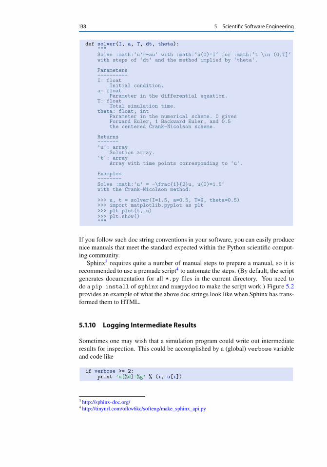
138 5 Scientific Software Engineering
def solver(I, a, T, dt, theta):"""Solve :math:‘u’=-au‘ with :math:‘u(0)=I‘ for :math:‘t \in (0,T]‘with steps of ‘dt‘ and the method implied by ‘theta‘.
Parameters----------I: float
Initial condition.a: float
Parameter in the differential equation.T: float
Total simulation time.theta: float, int
Parameter in the numerical scheme. 0 givesForward Euler, 1 Backward Euler, and 0.5the centered Crank-Nicolson scheme.
Returns-------‘u‘: array
Solution array.‘t‘: array
Array with time points corresponding to ‘u‘.
Examples--------Solve :math:‘u’ = -\frac{1}{2}u, u(0)=1.5‘with the Crank-Nicolson method:
>>> u, t = solver(I=1.5, a=0.5, T=9, theta=0.5)>>> import matplotlib.pyplot as plt>>> plt.plot(t, u)>>> plt.show()"""
If you follow such doc string conventions in your software, you can easily producenice manuals that meet the standard expected within the Python scientific comput-ing community.
Sphinx3 requires quite a number of manual steps to prepare a manual, so it isrecommended to use a premade script4 to automate the steps. (By default, the scriptgenerates documentation for all *.py files in the current directory. You need todo a pip install of sphinx and numpydoc to make the script work.) Figure 5.2provides an example of what the above doc strings look like when Sphinx has trans-formed them to HTML.
5.1.10 Logging Intermediate Results
Sometimes one may wish that a simulation program could write out intermediateresults for inspection. This could be accomplished by a (global) verbose variableand code like
if verbose >= 2:print ’u[%d]=%g’ % (i, u[i])
3 http://sphinx-doc.org/4 http://tinyurl.com/ofkw6kc/softeng/make_sphinx_api.py

5.1 Implementations with Functions and Modules 139
Fig. 5.2 Example on Sphinx API manual in HTML
The professional way to do report intermediate results and problems is, however, touse a logger. This is an object that writes messages to a log file. The messages areclassified as debug, info, and warning.
Introductory example Here is a simple example using defining a logger, usingPython’s logging module:
import logging# Configure loggerlogging.basicConfig(
filename=’myprog.log’, filemode=’w’, level=logging.WARNING,format=’%(asctime)s - %(levelname)s - %(message)s’,datefmt=’%m/%d/%Y %I:%M:%S %p’)
# Perform logginglogging.info(’Here is some general info.’)logging.warning(’Here is a warning.’)logging.debug(’Here is some debugging info.’)logging.critical(’Dividing by zero!’)logging.error(’Encountered an error.’)
Running this program gives the following output in the log file myprog.log:
09/26/2015 09:25:10 AM - INFO - Here is some general info.09/26/2015 09:25:10 AM - WARNING - Here is a warning.09/26/2015 09:25:10 AM - CRITICAL - Dividing by zero!09/26/2015 09:25:10 AM - ERROR - Encountered an error.
The logger has different levels of messages, ordered as critical, error, warning,info, and debug. The level argument to logging.basicConfig sets the level

140 5 Scientific Software Engineering
and thereby determines what the logger will print to the file: all messages at thespecified and lower levels are printed. For example, in the above example we setthe level to be info, and therefore the critical, error, warning, and info messageswere printed, but not the debug message. Setting level to debug (logging.DEBUG)prints all messages, while level critical prints only the critical messages.
The filemode argument is set to w such that any existing log file is overwritten(the default is a, which means append new messages to an existing log file, but thisis seldom what you want in mathematical computations).
The messages are preceded by the date and time and the level of the message.This output is governed by the format argument: asctime is the date and time,levelname is the name of the message level, and message is the message itself.Setting format=’%(message)s’ ensures that just the message and nothing moreis printed on each line. The datefmt string specifies the formatting of the date andtime, using the rules of the time.strftime5 function.
Using a logger in our solver function Let us let a logger write out intermediateresults and some debugging results in the solver function. Such messages areuseful for monitoring the simulation and for debugging it, respectively.
def solver_with_logging(I, a, T, dt, theta):"""Solve u’=-a*u, u(0)=I, for t in (0,T] with steps of dt."""dt = float(dt) # avoid integer divisionNt = int(round(T/dt)) # no of time intervalsT = Nt*dt # adjust T to fit time step dtu = np.zeros(Nt+1) # array of u[n] valuest = np.linspace(0, T, Nt+1) # time meshlogging.debug(’solver: dt=%g, Nt=%g, T=%g’ % (dt, Nt, T))
u[0] = I # assign initial conditionfor n in range(0, Nt): # n=0,1,...,Nt-1
u[n+1] = (1 - (1-theta)*a*dt)/(1 + theta*dt*a)*u[n]
logging.info(’u[%d]=%g’ % (n, u[n]))logging.debug(’1 - (1-theta)*a*dt: %g, %s’ %
(1-(1-theta)*a*dt,str(type(1-(1-theta)*a*dt))[7:-2]))
logging.debug(’1 + theta*dt*a: %g, %s’ %(1 + theta*dt*a,str(type(1 + theta*dt*a))[7:-2]))
return u, t
The application code that calls solver_with_logging needs to configure the log-ger. The decay module offers a default configure function:
import logging
def configure_basic_logger():logging.basicConfig(
filename=’decay.log’, filemode=’w’, level=logging.DEBUG,format=’%(asctime)s - %(levelname)s - %(message)s’,datefmt=’%Y.%m.%d %I:%M:%S %p’)
5 https://docs.python.org/2/library/time.html#time.strftime

5.1 Implementations with Functions and Modules 141
If the user of a library does not configure a logger or call this configure function,the library should prevent error messages by declaring a default logger that doesnothing:
import logginglogging.getLogger(’decay’).addHandler(logging.NullHandler())
We can run the new solver function with logging in a shell:
>>> import decay>>> decay.configure_basic_logger()>>> u, t = decay.solver_with_logging(I=1, a=0.5, T=10, \
dt=0.5, theta=0.5)
During this execution, each logging message is appended to the log file. Supposewe add some pause (time.sleep(2)) at each time level such that the executiontakes some time. In another terminal window we can then monitor the evolution ofdecay.log and the simulation by the tail -f Unix command:
Terminal> tail -f decay.log2015.09.26 05:37:41 AM - INFO - u[0]=12015.09.26 05:37:41 AM - INFO - u[1]=0.7777782015.09.26 05:37:41 AM - INFO - u[2]=0.6049382015.09.26 05:37:41 AM - INFO - u[3]=0.4705082015.09.26 05:37:41 AM - INFO - u[4]=0.365952015.09.26 05:37:41 AM - INFO - u[5]=0.284628
Especially in simulation where each time step demands considerable CPU time(minutes, hours), it can be handy to monitor such a log file to see the evolution ofthe simulation.
If we want to look more closely into the numerator and denominator of the for-mula for unC1, we can change the logging level to level=logging.DEBUG and getoutput in decay.log like
2015.09.26 05:40:01 AM - DEBUG - solver: dt=0.5, Nt=20, T=102015.09.26 05:40:01 AM - INFO - u[0]=12015.09.26 05:40:01 AM - DEBUG - 1 - (1-theta)*a*dt: 0.875, float2015.09.26 05:40:01 AM - DEBUG - 1 + theta*dt*a: 1.125, float2015.09.26 05:40:01 AM - INFO - u[1]=0.7777782015.09.26 05:40:01 AM - DEBUG - 1 - (1-theta)*a*dt: 0.875, float2015.09.26 05:40:01 AM - DEBUG - 1 + theta*dt*a: 1.125, float2015.09.26 05:40:01 AM - INFO - u[2]=0.6049382015.09.26 05:40:01 AM - DEBUG - 1 - (1-theta)*a*dt: 0.875, float2015.09.26 05:40:01 AM - DEBUG - 1 + theta*dt*a: 1.125, float2015.09.26 05:40:01 AM - INFO - u[3]=0.4705082015.09.26 05:40:01 AM - DEBUG - 1 - (1-theta)*a*dt: 0.875, float2015.09.26 05:40:01 AM - DEBUG - 1 + theta*dt*a: 1.125, float2015.09.26 05:40:01 AM - INFO - u[4]=0.365952015.09.26 05:40:01 AM - DEBUG - 1 - (1-theta)*a*dt: 0.875, float2015.09.26 05:40:01 AM - DEBUG - 1 + theta*dt*a: 1.125, float
Logging can be much more sophisticated than shown above. One can, e.g., out-put critical messages to the screen and all messages to a file. This requires morecode as demonstrated in the Logging Cookbook6.
6 https://docs.python.org/2/howto/logging-cookbook.html

142 5 Scientific Software Engineering
5.2 User Interfaces
It is good programming practice to let programs read input from some user inter-face, rather than requiring users to edit parameter values in the source code. Witheffective user interfaces it becomes easier and safer to apply the code for scien-tific investigations and in particular to automate large-scale investigations by otherprograms (see Sect. 5.6).
Reading input data can be done in many ways. We have to decide on the func-tionality of the user interface, i.e., how we want to operate the program whenproviding input. Thereafter, we use appropriate tools to implement the particularuser interface. There are four basic types of user interface, listed here according toimplementational complexity, from lowest to highest:
1. Questions and answers in the terminal window2. Command-line arguments3. Reading data from files4. Graphical user interfaces (GUIs)
Personal preferences of user interfaces differ substantially, and it is difficult topresent recommendations or pros and cons. Alternatives 2 and 4 are most popularand will be addressed next. The goal is to make it easy for the user to set physicaland numerical parameters in our decay.py program. However, we use a little toyprogram, called prog.py, as introductory example:
delta = 0.5p = 2from math import expresult = delta*exp(-p)print result
The essential content is that prog.py has two input parameters: delta and p.A user interface will replace the first two assignments to delta and p.
5.2.1 Command-Line Arguments
The command-line arguments are all the words that appear on the command lineafter the program name. Running a program prog.py as python prog.py arg1arg2 means that there are two command-line arguments (separated by whitespace): arg1 and arg2. Python stores all command-line arguments in a special listsys.argv. (The name argv stems from the C language and stands for “argumentvalues”. In C there is also an integer variable called argc reflecting the number ofarguments, or “argument counter”. A lot of programming languages have adoptedthe variable name argv for the command-line arguments.) Here is an exampleon a program what_is_sys_argv.py that can show us what the command-linearguments are
import sysprint sys.argv

5.2 User Interfaces 143
A sample run goes like
Terminal
Terminal> python what_is_sys_argv.py 5.0 ’two words’ -1E+4[’what_is_sys_argv.py’, ’5.0’, ’two words’, ’-1E+4’]
We make two observations:
� sys.argv[0] is the name of the program, and the sublist sys.argv[1:] con-tains all the command-line arguments.
� Each command-line argument is available as a string. A conversion to float isnecessary if we want to compute with the numbers 5.0 and 104.
There are, in principle, two ways of programming with command-line arguments inPython:
� Positional arguments: Decide upon a sequence of parameters on the commandline and read their values directly from the sys.argv[1:] list.
� Option-value pairs: Use –option value on the command line to replacethe default value of an input parameter option by value (and utilize theargparse.ArgumentParser tool for implementation).
Suppose we want to run some program prog.py with specification of two param-eters p and delta on the command line. With positional command-line argumentswe write
Terminal
Terminal> python prog.py 2 0.5
and must know that the first argument 2 represents p and the next 0.5 is the valueof delta. With option-value pairs we can run
Terminal
Terminal> python prog.py --delta 0.5 --p 2
Now, both p and delta are supposed to have default values in the program, sowe need to specify only the parameter that is to be changed from its default value,e.g.,
Terminal
Terminal> python prog.py --p 2 # p=2, default deltaTerminal> python prog.py --delta 0.7 # delta-0.7, default aTerminal> python prog.py # default a and delta
How do we extend the prog.py code for positional arguments and option-valuepairs? Positional arguments require very simple code:

144 5 Scientific Software Engineering
import sysp = float(sys.argv[1])delta = float(sys.argv[2])
from math import expresult = delta*exp(-p)print result
If the user forgets to supply two command-line arguments, Python will raise anIndexError exception and produce a long error message. To avoid that, we shoulduse a try-except construction:
import systry:
p = float(sys.argv[1])delta = float(sys.argv[2])
except IndexError:print ’Usage: %s p delta’ % sys.argv[0]sys.exit(1)
from math import expresult = delta*exp(-p)print result
Using sys.exit(1) aborts the program. The value 1 (actually any value differentfrom 0) notifies the operating system that the program failed.
Command-line arguments are strings!Note that all elements in sys.argv are string objects. If the values are used inmathematical computations, we need to explicitly convert the strings to numbers.
Option-value pairs requires more programming and is actually better explainedin a more comprehensive example below. Minimal code for our prog.py programreads
import argparseparser = argparse.ArgumentParser()parser.add_argument(’--p’, default=1.0)parser.add_argument(’--delta’, default=0.1)
args = parser.parse_args()p = args.pdelta = args.delta
from math import expresult = delta*exp(-p)print result
Because the default values of delta and p are float numbers, the args.delta andargs.p variables are automatically of type float.
Our next task is to use these basic code constructs to equip our decay.pymodulewith command-line interfaces.

5.2 User Interfaces 145
5.2.2 Positional Command-Line Arguments
For our decay.py module file, we want to include functionality such that we canread I , a, T , � , and a range of �t values from the command line. A plot is then to bemade, comparing the different numerical solutions for different �t values againstthe exact solution. The technical details of getting the command-line informationinto the program is covered in the next two sections.
The simplest way of reading the input parameters is to decide on their sequenceon the command line and just index the sys.argv list accordingly. Say the se-quence of input data for some functionality in decay.py is I , a, T , � followed byan arbitrary number of �t values. This code extracts these positional command-linearguments:
def read_command_line_positional():if len(sys.argv) < 6:
print ’Usage: %s I a T on/off BE/FE/CN dt1 dt2 dt3 ...’ % \sys.argv[0]; sys.exit(1) # abort
I = float(sys.argv[1])a = float(sys.argv[2])T = float(sys.argv[3])theta = float(sys.argv[4])dt_values = [float(arg) for arg in sys.argv[5:]]
return I, a, T, theta, dt_values
Note that we may use a try-except construction instead of the if test.A run like
Terminal
Terminal> python decay.py 1 0.5 4 0.5 1.5 0.75 0.1
results in
sys.argv = [’decay.py’, ’1’, ’0.5’, ’4’, ’0.5’, ’1.5’, ’0.75’, ’0.1’]
and consequently the assignments I=1.0, a=0.5, T=4.0, thet=0.5, anddt_values = [1.5, 0.75, 0.1].
Instead of specifying the � value, we could be a bit more sophisticated and let theuser write the name of the scheme: BE for Backward Euler, FE for Forward Euler,and CN for Crank–Nicolson. Then we must map this string to the proper � value, anoperation elegantly done by a dictionary:
scheme = sys.argv[4]scheme2theta = {’BE’: 1, ’CN’: 0.5, ’FE’: 0}if scheme in scheme2theta:
theta = scheme2theta[scheme]else:
print ’Invalid scheme name:’, scheme; sys.exit(1)

146 5 Scientific Software Engineering
Now we can do
Terminal
Terminal> python decay.py 1 0.5 4 CN 1.5 0.75 0.1
and get ‘theta=0.5‘in the code.
5.2.3 Option-Value Pairs on the Command Line
Now we want to specify option-value pairs on the command line, using –I for I (I ),–a for a (a), –T for T (T ), –scheme for the scheme name (BE, FE, CN), and –dt forthe sequence of dt (�t) values. Each parameter must have a sensible default valueso that we specify the option on the command line only when the default value isnot suitable. Here is a typical run:
Terminal
Terminal> python decay.py --I 2.5 --dt 0.1 0.2 0.01 --a 0.4
Observe the major advantage over positional command-line arguments: the inputis much easier to read and much easier to write. With positional arguments it is easyto mess up the sequence of the input parameters and quite challenging to detecterrors too, unless there are just a couple of arguments.
Python’s ArgumentParser tool in the argparse module makes it easy to cre-ate a professional command-line interface to any program. The documentationof ArgumentParser7 demonstrates its versatile applications, so we shall herejust list an example containing the most basic features. It always pays off to useArgumentParser rather than trying to manually inspect and interpret option-valuepairs in sys.argv!
The use of ArgumentParser typically involves three steps:
import argparseparser = argparse.ArgumentParser()
# Step 1: add argumentsparser.add_argument(’--option_name’, ...)
# Step 2: interpret the command lineargs = parser.parse_args()
# Step 3: extract valuesvalue = args.option_name
7 http://docs.python.org/library/argparse.html

5.2 User Interfaces 147
A function for setting up all the options is handy:
def define_command_line_options():import argparseparser = argparse.ArgumentParser()parser.add_argument(
’--I’, ’--initial_condition’, type=float,default=1.0, help=’initial condition, u(0)’,metavar=’I’)
parser.add_argument(’--a’, type=float, default=1.0,help=’coefficient in ODE’, metavar=’a’)
parser.add_argument(’--T’, ’--stop_time’, type=float,default=1.0, help=’end time of simulation’,metavar=’T’)
parser.add_argument(’--scheme’, type=str, default=’CN’,help=’FE, BE, or CN’)
parser.add_argument(’--dt’, ’--time_step_values’, type=float,default=[1.0], help=’time step values’,metavar=’dt’, nargs=’+’, dest=’dt_values’)
return parser
Each command-line option is defined through the parser.add_argumentmethod8. Alternative options, like the short –I and the more explaining version--initial_condition can be defined. Other arguments are type for the Pythonobject type, a default value, and a help string, which gets printed if the command-line argument -h or –help is included. The metavar argument specifies the valueassociated with the option when the help string is printed. For example, the optionfor I has this help output:
Terminal
Terminal> python decay.py -h...--I I, --initial_condition I
initial condition, u(0)...
The structure of this output is
--I metavar, --initial_condition metavarhelp-string
Finally, the –dt option demonstrates how to allow for more than one value (sep-arated by blanks) through the nargs=’+’ keyword argument. After the commandline is parsed, we get an object where the values of the options are stored as at-tributes. The attribute name is specified by the dist keyword argument, which forthe –dt option is dt_values. Without the dest argument, the value of an option–opt is stored as the attribute opt.
8 We use the expression method here, because parser is a class variable and functions in classesare known as methods in Python and many other languages. Readers not familiar with classprogramming can just substitute this use of method by function.

148 5 Scientific Software Engineering
The code below demonstrates how to read the command line and extract thevalues for each option:
def read_command_line_argparse():parser = define_command_line_options()args = parser.parse_args()scheme2theta = {’BE’: 1, ’CN’: 0.5, ’FE’: 0}data = (args.I, args.a, args.T, scheme2theta[args.scheme],
args.dt_values)return data
As seen, the values of the command-line options are available as attributes in args:args.opt holds the value of option –opt, unless we used the dest argument (asfor --dt_values) for specifying the attribute name. The args.opt attribute hasthe object type specified by type (str by default).
The making of the plot is not dependent on whether we read data from the com-mand line as positional arguments or option-value pairs:
def experiment_compare_dt(option_value_pairs=False):I, a, T, theta, dt_values = \
read_command_line_argparse() if option_value_pairs else \read_command_line_positional()
legends = []for dt in dt_values:
u, t = solver(I, a, T, dt, theta)plt.plot(t, u)legends.append(’dt=%g’ % dt)
t_e = np.linspace(0, T, 1001) # very fine mesh for u_eu_e = u_exact(t_e, I, a)plt.plot(t_e, u_e, ’--’)legends.append(’exact’)plt.legend(legends, loc=’upper right’)plt.title(’theta=%g’ % theta)plotfile = ’tmp’plt.savefig(plotfile + ’.png’); plt.savefig(plotfile + ’.pdf’)
5.2.4 Creating a Graphical Web User Interface
The Python package Parampool9 can be used to automatically generate a web-basedgraphical user interface (GUI) for our simulation program. Although the program-ming technique dramatically simplifies the efforts to create a GUI, the forthcomingmaterial on equipping our decay module with a GUI is quite technical and of sig-nificantly less importance than knowing how to make a command-line interface.
Making a compute function The first step is to identify a function that performsthe computations and that takes the necessary input variables as arguments. This iscalled the compute function in Parampool terminology. The purpose of this functionis to take values of I , a, T together with a sequence of �t values and a sequenceof � and plot the numerical against the exact solution for each pair of .�; �t/. Theplots can be arranged as a table with the columns being scheme type (� value) and
9 https://github.com/hplgit/parampool

5.2 User Interfaces 149
Fig. 5.3 Automatically generated graphical web interface
the rows reflecting the discretization parameter (�t value). Figure 5.3 displays whatthe graphical web interface may look like after results are computed (there are 33
plots in the GUI, but only 2 2 are visible in the figure).To tell Parampool what type of input data we have, we assign default values of
the right type to all arguments in the compute function, here called main_GUI:
def main_GUI(I=1.0, a=.2, T=4.0,dt_values=[1.25, 0.75, 0.5, 0.1],theta_values=[0, 0.5, 1]):
The compute function must return the HTML code we want for displaying theresult in a web page. Here we want to show a table of plots. Assume for now thatthe HTML code for one plot and the value of the norm of the error can be computedby some other function compute4web. The main_GUI function can then loop over�t and � values and put each plot in an HTML table. Appropriate code goes like
def main_GUI(I=1.0, a=.2, T=4.0,dt_values=[1.25, 0.75, 0.5, 0.1],theta_values=[0, 0.5, 1]):
# Build HTML code for web page. Arrange plots in columns# corresponding to the theta values, with dt down the rowstheta2name = {0: ’FE’, 1: ’BE’, 0.5: ’CN’}html_text = ’<table>\n’for dt in dt_values:
html_text += ’<tr>\n’for theta in theta_values:
E, html = compute4web(I, a, T, dt, theta)html_text += """

150 5 Scientific Software Engineering
<td><center><b>%s, dt=%g, error: %.3E</b></center><br>%s</td>""" % (theta2name[theta], dt, E, html)
html_text += ’</tr>\n’html_text += ’</table>\n’return html_text
Making one plot is done in compute4web. The statements should be straightfor-ward from earlier examples, but there is one new feature: we use a tool in Parampoolto embed the PNG code for a plot file directly in an HTML image tag. The detailsare hidden from the programmer, who can just rely on relevant HTML code in thestring html_text. The function looks like
def compute4web(I, a, T, dt, theta=0.5):"""Run a case with the solver, compute error measure,and plot the numerical and exact solutions in a PNGplot whose data are embedded in an HTML image tag."""u, t = solver(I, a, T, dt, theta)u_e = u_exact(t, I, a)e = u_e - uE = np.sqrt(dt*np.sum(e**2))
plt.figure()t_e = np.linspace(0, T, 1001) # fine mesh for u_eu_e = u_exact(t_e, I, a)plt.plot(t, u, ’r--o’)plt.plot(t_e, u_e, ’b-’)plt.legend([’numerical’, ’exact’])plt.xlabel(’t’)plt.ylabel(’u’)plt.title(’theta=%g, dt=%g’ % (theta, dt))# Save plot to HTML img tag with PNG code as embedded datafrom parampool.utils import save_png_to_strhtml_text = save_png_to_str(plt, plotwidth=400)
return E, html_text
Generating the user interface The web GUI is automatically generated by thefollowing code, placed in the file decay_GUI_generate.py10.
from parampool.generator.flask import generatefrom decay import main_GUIgenerate(main_GUI,
filename_controller=’decay_GUI_controller.py’,filename_template=’decay_GUI_view.py’,filename_model=’decay_GUI_model.py’)
Running the decay_GUI_generate.py program results in three new files whosenames are specified in the call to generate:
1. decay_GUI_model.py defines HTML widgets to be used to set input data inthe web interface,
10 http://tinyurl.com/ofkw6kc/softeng/decay_GUI_generate.py

5.3 Tests for Verifying Implementations 151
2. templates/decay_GUI_views.py defines the layout of the web page,3. decay_GUI_controller.py runs the web application.
We only need to run the last program, and there is no need to look into these files.
Running the web application The web GUI is started by
Terminal
Terminal> python decay_GUI_controller.py
Open a web browser at the location 127.0.0.1:5000. Input fields for I, a, T,dt_values, and theta_values are presented. Figure 5.3 shows a part of the re-sulting page if we run with the default values for the input parameters. With thetechniques demonstrated here, one can easily create a tailored web GUI for a par-ticular type of application and use it to interactively explore physical and numericaleffects.
5.3 Tests for Verifying Implementations
Any module with functions should have a set of tests that can check the correctnessof the implementations. There exists well-established procedures and correspond-ing tools for automating the execution of such tests. These tools allow large test setsto be run with a one-line command, making it easy to check that the software stillworks (as far as the tests can tell!). Here we shall illustrate two important softwaretesting techniques: doctest and unit testing. The first one is Python specific, whileunit testing is the dominating test technique in the software industry today.
5.3.1 Doctests
A doc string, the first string after the function header, is used to document the pur-pose of functions and their arguments (see Sect. 5.1.5). Very often it is instructiveto include an example in the doc string on how to use the function. Interactiveexamples in the Python shell are most illustrative as we can see the output result-ing from the statements and expressions. For example, in the solver function, wecan include an example on calling this function and printing the computed u and tarrays:
def solver(I, a, T, dt, theta):"""Solve u’=-a*u, u(0)=I, for t in (0,T] with steps of dt.
>>> u, t = solver(I=0.8, a=1.2, T=1.5, dt=0.5, theta=0.5)>>> for n in range(len(t)):... print ’t=%.1f, u=%.14f’ % (t[n], u[n])t=0.0, u=0.80000000000000t=0.5, u=0.43076923076923

152 5 Scientific Software Engineering
t=1.0, u=0.23195266272189t=1.5, u=0.12489758761948"""...
When such interactive demonstrations are inserted in doc strings, Python’sdoctest11 module can be used to automate running all commands in interactivesessions and compare new output with the output appearing in the doc string. Allwe have to do in the current example is to run the module file decay.py with
Terminal> python -m doctest decay.py
This command imports the doctest module, which runs all doctests found in thefile and reports discrepancies between expected and computed output. Alterna-tively, the test block in a module may run all doctests by
if __name__ == ’__main__’:import doctestdoctest.testmod()
Doctests can also be embedded in nose/pytest unit tests as explained in the nextsection.
Doctests prevent command-line arguments!No additional command-line argument is allowed when running doctests. If yourprogram relies on command-line input, make sure the doctests can be run withoutsuch input on the command line.
However, you can simulate command-line input by filling sys.argv withvalues, e.g.,
import sys; sys.argv = ’--I 1.0 --a 5’.split()
The execution command above will report any problem if a test fails. As anillustration, let us alter the u value at t=1.5 in the output of the doctest by replacingthe last digit 8 by 7. This edit triggers a report:
Terminal
Terminal> python -m doctest decay.py********************************************************File "decay.py", line ...Failed example:
for n in range(len(t)):print ’t=%.1f, u=%.14f’ % (t[n], u[n])
Expected:t=0.0, u=0.80000000000000t=0.5, u=0.43076923076923t=1.0, u=0.23195266272189t=1.5, u=0.12489758761948
Got:t=0.0, u=0.80000000000000t=0.5, u=0.43076923076923
11 http://docs.python.org/library/doctest.html

5.3 Tests for Verifying Implementations 153
t=1.0, u=0.23195266272189t=1.5, u=0.12489758761947
Pay attention to the number of digits in doctest results!Note that in the output of t and u we write u with 14 digits. Writing all 16digits is not a good idea: if the tests are run on different hardware, round-offerrors might be different, and the doctest module detects that the numbers arenot precisely the same and reports failures. In the present application, where0 < u.t/ � 0:8, we expect round-off errors to be of size 10�16, so comparing 15digits would probably be reliable, but we compare 14 to be on the safe side. Onthe other hand, comparing a small number of digits may hide software errors.
Doctests are highly encouraged as they do two things: 1) demonstrate howa function is used and 2) test that the function works.
5.3.2 Unit Tests and Test Functions
The unit testing technique consists of identifying smaller units of code and writ-ing one or more tests for each unit. One unit can typically be a function. Eachtest should, ideally, not depend on the outcome of other tests. The recommendedpractice is actually to design and write the unit tests first and then implement thefunctions!
In scientific computing it is not always obvious how to best perform unit testing.The units are naturally larger than in non-scientific software. Very often the solutionprocedure of a mathematical problem identifies a unit, such as our solver function.
Two Python test frameworks: nose and pytest Python offers two very easy-to-use software frameworks for implementing unit tests: nose and pytest. These work(almost) in the same way, but our recommendation is to go for pytest.
Test function requirements For a test to qualify as a test function in nose or pytest,three rules must be followed:
1. The function name must start with test_.2. Function arguments are not allowed.3. An AssertionError exception must be raised if the test fails.
A specific example might be illustrative before proceeding. We have the followingfunction that we want to test:
def double(n):return 2*n
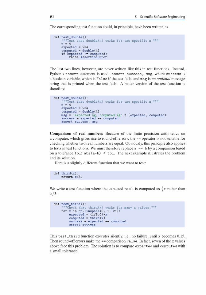
154 5 Scientific Software Engineering
The corresponding test function could, in principle, have been written as
def test_double():"""Test that double(n) works for one specific n."""n = 4expected = 2*4computed = double(4)if expected != computed:
raise AssertionError
The last two lines, however, are never written like this in test functions. Instead,Python’s assert statement is used: assert success, msg, where success isa boolean variable, which is False if the test fails, and msg is an optional messagestring that is printed when the test fails. A better version of the test function istherefore
def test_double():"""Test that double(n) works for one specific n."""n = 4expected = 2*4computed = double(4)msg = ’expected %g, computed %g’ % (expected, computed)success = expected == computedassert success, msg
Comparison of real numbers Because of the finite precision arithmetics ona computer, which gives rise to round-off errors, the == operator is not suitable forchecking whether two real numbers are equal. Obviously, this principle also appliesto tests in test functions. We must therefore replace a == b by a comparison basedon a tolerance tol: abs(a-b) < tol. The next example illustrates the problemand its solution.
Here is a slightly different function that we want to test:
def third(x):return x/3.
We write a test function where the expected result is computed as 13x rather than
x=3:
def test_third():"""Check that third(x) works for many x values."""for x in np.linspace(0, 1, 21):
expected = (1/3.0)*xcomputed = third(x)success = expected == computedassert success
This test_third function executes silently, i.e., no failure, until x becomes 0.15.Then round-off errors make the == comparison False. In fact, seven of the x valuesabove face this problem. The solution is to compare expected and computed witha small tolerance:

5.3 Tests for Verifying Implementations 155
def test_third():"""Check that third(x) works for many x values."""for x in np.linspace(0, 1, 21):
expected = (1/3.)*xcomputed = third(x)tol = 1E-15success = abs(expected - computed) < tolassert success
Always compare real numbers with a tolerance!Real numbers should never be compared with the == operator, but always withthe absolute value of the difference and a tolerance. So, replace a == b, if aand/or b is float, by
tol = 1E-14abs(a - b) < tol
The suitable size of tol depends on the size of a and b (see Problem 5.5). Unlessa and b are around unity in size, one should use a relative difference:
tol = 1E-14abs((a - b)/a) < tol
Special assert functions from nose Test frameworks often contain more tailoredassert functions that can be called instead of using the assert statement. For ex-ample, comparing two objects within a tolerance, as in the present case, can be doneby the assert_almost_equal from the nose framework:
import nose.tools as nt
def test_third():x = 0.15expected = (1/3.)*xcomputed = third(x)nt.assert_almost_equal(
expected, computed, delta=1E-15,msg=’diff=%.17E’ % (expected - computed))
Whether to use the plain assert statement with a comparison based on a tol-erance or to use the ready-made function assert_almost_equal depends on theprogrammer’s preference. The examples used in the documentation of the pytestframework stick to the plain assert statement.
Locating test functions Test functions can reside in a module together with thefunctions they are supposed to verify, or the test functions can be collected in sepa-rate files having names starting with test. Actually, nose and pytest can recursivelyrun all test functions in all test*.py files in the current directory, as well as in allsubdirectories!

156 5 Scientific Software Engineering
The decay.py12 module file features test functions in the module, but wecould equally well have made a subdirectory tests and put the test functions intests/test_decay.py13.
Running tests To run all test functions in the file decay.py do
Terminal
Terminal> nosetests -s -v decay.pyTerminal> py.test -s -v decay.py
The -s option ensures that output from the test functions is printed in the termi-nal window, while -v prints the outcome of each individual test function.
Alternatively, if the test functions are located in some separate test*.py files,we can just write
Terminal
Terminal> py.test -s -v
to recursively run all test functions in the current directory tree. The corresponding
Terminal
Terminal> nosetests -s -v
command does the same, but requires subdirectory names to start with test or endwith _test or _tests (which is a good habit anyway). An example of a testsdirectory with a test*.py file is found in src/softeng/tests14.
Embedding doctests in a test function Doctests can also be executed fromnose/pytest unit tests. Here is an example of a file test_decay_doctest.py15
where we in the test block run all the doctests in the imported module decay, butwe also include a local test function that does the same:
import sys, ossys.path.insert(0, os.pardir)import decayimport doctest
def test_decay_module_with_doctest():"""Doctest embedded in a nose/pytest unit test."""# Test all functions with doctest in module decayfailure_count, test_count = doctest.testmod(m=decay)assert failure_count == 0
if __name__ == ’__main__’:# Run all functions with doctests in this modulefailure_count, test_count = doctest.testmod(m=decay)
12 http://tinyurl.com/ofkw6kc/softeng/decay.py13 http://tinyurl.com/ofkw6kc/softeng/tests/test_decay.py14 http://tinyurl.com/ofkw6kc/softeng/tests15 http://tinyurl.com/ofkw6kc/softeng/tests/test_decay_doctest.py

5.3 Tests for Verifying Implementations 157
Running this file as a program from the command line triggers the doctest.testmod call in the test block, while applying py.test or nosetests to the filetriggers an import of the file and execution of the test functiontest_decay_modue_with_doctest.
Installing nose and pytest With pip available, it is trivial to install nose and/orpytest: sudo pip install nose and sudo pip install pytest.
5.3.3 Test Function for the Solver
Finding good test problems for verifying the implementation of numerical methodsis a topic on its own. The challenge is that we very seldom know what the numericalerrors are. For the present model problem (5.1)–(5.2) solved by (5.3) one can,fortunately, derive a formula for the numerical approximation:
un D I
�1 � .1 � �/a�t
1C �a�t
�n
:
Then we know that the implementation should produce numbers that agree withthis formula to machine precision. The formula for un is known as an exact discretesolution of the problem and can be coded as
def u_discrete_exact(n, I, a, theta, dt):"""Return exact discrete solution of the numerical schemes."""dt = float(dt) # avoid integer divisionA = (1 - (1-theta)*a*dt)/(1 + theta*dt*a)return I*A**n
A test function can evaluate this solution on a time mesh and check that the u valuesproduced by the solver function do not deviate with more than a small tolerance:
def test_u_discrete_exact():"""Check that solver reproduces the exact discr. sol."""theta = 0.8; a = 2; I = 0.1; dt = 0.8Nt = int(8/dt) # no of stepsu, t = solver(I=I, a=a, T=Nt*dt, dt=dt, theta=theta)
# Evaluate exact discrete solution on the meshu_de = np.array([u_discrete_exact(n, I, a, theta, dt)
for n in range(Nt+1)])
# Find largest deviationdiff = np.abs(u_de - u).max()tol = 1E-14success = diff < tolassert success
Among important things to consider when constructing test functions is testingthe effect of wrong input to the function being tested. In our solver function, forexample, integer values of a, �t , and � may cause unintended integer division. We

158 5 Scientific Software Engineering
should therefore add a test to make sure our solver function does not fall into thispotential trap:
def test_potential_integer_division():"""Choose variables that can trigger integer division."""theta = 1; a = 1; I = 1; dt = 2Nt = 4u, t = solver(I=I, a=a, T=Nt*dt, dt=dt, theta=theta)u_de = np.array([u_discrete_exact(n, I, a, theta, dt)
for n in range(Nt+1)])diff = np.abs(u_de - u).max()assert diff < 1E-14
In more complicated problems where there is no exact solution of the numericalproblem solved by the software, one must use the method of manufactured solu-tions, compute convergence rates for a series of �t values, and check that the ratesconverges to the expected ones (from theory). This type of testing is fully explainedin Sect. 3.1.6.
5.3.4 Test Function for Reading Positional Command-LineArguments
The function read_command_line_positional extracts numbers from the com-mand line. To test it, we must decide on a set of values for the input data, fillsys.argv accordingly, and check that we get the expected values:
def test_read_command_line_positional():# Decide on a data set of input parametersI = 1.6; a = 1.8; T = 2.2; theta = 0.5dt_values = [0.1, 0.2, 0.05]# Expected return from read_command_line_positionalexpected = [I, a, T, theta, dt_values]# Construct corresponding sys.argv arraysys.argv = [sys.argv[0], str(I), str(a), str(T), ’CN’] + \
[str(dt) for dt in dt_values]computed = read_command_line_positional()for expected_arg, computed_arg in zip(expected, computed):
assert expected_arg == computed_arg
Note that sys.argv[0] is always the program name and that we have to copy thatstring from the original sys.argv array to the new one we construct in the testfunction. (Actually, this test function destroys the original sys.argv that Pythonfetched from the command line.)
Any numerical code writer should always be skeptical to the use of the exactequality operator == in test functions, since round-off errors often come into play.Here, however, we set some real values, convert them to strings and convert backagain to real numbers (of the same precision). This string-number conversion doesnot involve any finite precision arithmetics effects so we can safely use == in tests.Note also that the last element in expected and computed is the list dt_values,and == works for comparing two lists as well.

5.3 Tests for Verifying Implementations 159
5.3.5 Test Function for Reading Option-Value Pairs
The function read_command_line_argparse can be verified with a test functionthat has the same setup as test_read_command_line_positional above. How-ever, the construction of the command line is a bit more complicated. We find itconvenient to construct the line as a string and then split the line into words to getthe desired list sys.argv:
def test_read_command_line_argparse():I = 1.6; a = 1.8; T = 2.2; theta = 0.5dt_values = [0.1, 0.2, 0.05]# Expected return from read_command_line_argparseexpected = [I, a, T, theta, dt_values]# Construct corresponding sys.argv arraycommand_line = ’%s --a %s --I %s --T %s --scheme CN --dt ’ % \
(sys.argv[0], a, I, T)command_line += ’ ’.join([str(dt) for dt in dt_values])sys.argv = command_line.split()computed = read_command_line_argparse()for expected_arg, computed_arg in zip(expected, computed):
assert expected_arg == computed_arg
Recall that the Python function zip enables iteration over several lists, tuples, orarrays at the same time.
Let silent test functions speak up during development!When you develop test functions in a module, it is common to use IPython forinteractive experimentation:
In[1]: import decay
In[2]: decay.test_read_command_line_argparse()
Note that a working test function is completely silent! Many find it psycho-logically annoying to convince themselves that a completely silent function isdoing the right things. It can therefore, during development of a test function, beconvenient to insert print statements in the function to monitor that the functionbody is indeed executed. For example, one can print the expected and computedvalues in the terminal window:
def test_read_command_line_argparse():...for expected_arg, computed_arg in zip(expected, computed):
print expected_arg, computed_argassert expected_arg == computed_arg
After performing this edit, we want to run the test again, but in IPython themodule must first be reloaded (reimported):
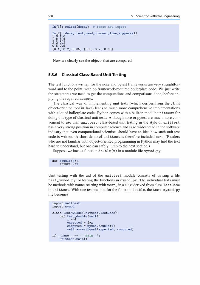
160 5 Scientific Software Engineering
In[3]: reload(decay) # force new import
In[2]: decay.test_read_command_line_argparse()1.6 1.61.8 1.82.2 2.20.5 0.5[0.1, 0.2, 0.05] [0.1, 0.2, 0.05]
Now we clearly see the objects that are compared.
5.3.6 Classical Class-Based Unit Testing
The test functions written for the nose and pytest frameworks are very straightfor-ward and to the point, with no framework-required boilerplate code. We just writethe statements we need to get the computations and comparisons done, before ap-plying the required assert.
The classical way of implementing unit tests (which derives from the JUnitobject-oriented tool in Java) leads to much more comprehensive implementationswith a lot of boilerplate code. Python comes with a built-in module unittest fordoing this type of classical unit tests. Although nose or pytest are much more con-venient to use than unittest, class-based unit testing in the style of unittesthas a very strong position in computer science and is so widespread in the softwareindustry that even computational scientists should have an idea how such unit testcode is written. A short demo of unittest is therefore included next. (Readerswho are not familiar with object-oriented programming in Python may find the texthard to understand, but one can safely jump to the next section.)
Suppose we have a function double(x) in a module file mymod.py:
def double(x):return 2*x
Unit testing with the aid of the unittest module consists of writing a filetest_mymod.py for testing the functions in mymod.py. The individual tests mustbe methods with names starting with test_ in a class derived from class TestCasein unittest. With one test method for the function double, the test_mymod.pyfile becomes
import unittestimport mymod
class TestMyCode(unittest.TestCase):def test_double(self):
x = 4expected = 2*xcomputed = mymod.double(x)self.assertEqual(expected, computed)
if __name__ == ’__main__’:unittest.main()
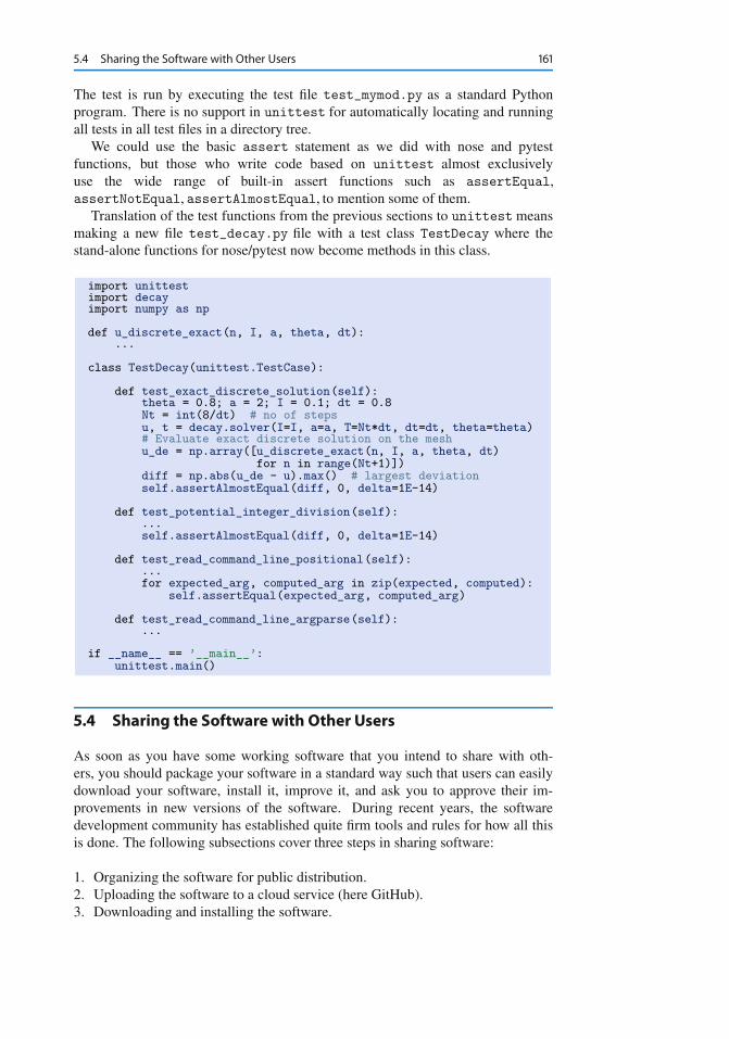
5.4 Sharing the Software with Other Users 161
The test is run by executing the test file test_mymod.py as a standard Pythonprogram. There is no support in unittest for automatically locating and runningall tests in all test files in a directory tree.
We could use the basic assert statement as we did with nose and pytestfunctions, but those who write code based on unittest almost exclusivelyuse the wide range of built-in assert functions such as assertEqual,assertNotEqual, assertAlmostEqual, to mention some of them.
Translation of the test functions from the previous sections to unittest meansmaking a new file test_decay.py file with a test class TestDecay where thestand-alone functions for nose/pytest now become methods in this class.
import unittestimport decayimport numpy as np
def u_discrete_exact(n, I, a, theta, dt):...
class TestDecay(unittest.TestCase):
def test_exact_discrete_solution(self):theta = 0.8; a = 2; I = 0.1; dt = 0.8Nt = int(8/dt) # no of stepsu, t = decay.solver(I=I, a=a, T=Nt*dt, dt=dt, theta=theta)# Evaluate exact discrete solution on the meshu_de = np.array([u_discrete_exact(n, I, a, theta, dt)
for n in range(Nt+1)])diff = np.abs(u_de - u).max() # largest deviationself.assertAlmostEqual(diff, 0, delta=1E-14)
def test_potential_integer_division(self):...self.assertAlmostEqual(diff, 0, delta=1E-14)
def test_read_command_line_positional(self):...for expected_arg, computed_arg in zip(expected, computed):
self.assertEqual(expected_arg, computed_arg)
def test_read_command_line_argparse(self):...
if __name__ == ’__main__’:unittest.main()
5.4 Sharing the Software with Other Users
As soon as you have some working software that you intend to share with oth-ers, you should package your software in a standard way such that users can easilydownload your software, install it, improve it, and ask you to approve their im-provements in new versions of the software. During recent years, the softwaredevelopment community has established quite firm tools and rules for how all thisis done. The following subsections cover three steps in sharing software:
1. Organizing the software for public distribution.2. Uploading the software to a cloud service (here GitHub).3. Downloading and installing the software.

162 5 Scientific Software Engineering
5.4.1 Organizing the Software Directory Tree
We start with organizing our software as a directory tree. Our software consists ofone module file, decay.py, and possibly some unit tests in a separate file locatedin a directory tests.
The decay.py can be used as a module or as a program. For distribution to otherusers who install the program decay.py in system directories, we need to insert thefollowing line at the top of the file:
#!/usr/bin/env python
This line makes it possible to write just the filename and get the file executed bythe python program (or more precisely, the first python program found in thedirectories in the PATH environment variable).
Distributing just a module file Let us start out with the minimum solution alter-native: distributing just the decay.py file. Then the software is just one file and allwe need is a directory with this file. This directory will also contain an installationscript setup.py and a README file telling what the software is about, the author’semail address, a URL for downloading the software, and other useful information.
The setup.py file can be as short as
from distutils.core import setupsetup(name=’decay’,
version=’0.1’,py_modules=[’decay’],scripts=[’decay.py’],)
The py_modules argument specifies a list of modules to be installed, whilescripts specifies stand-alone programs. Our decay.py can be used either asa module or as an executable program, so we want users to have both possibilities.
Distributing a package If the software consists of more files than one or two mod-ules, one should make a Python package out of it. In our case we make a packagedecay containing one module, also called decay.
To make a package decay, create a directory decay and an empty file in it withname __init__.py. A setup.py script must now specify the directory name ofthe package and also an executable program (scripts=) in case we want to rundecay.py as a stand-alone application:
from distutils.core import setupimport os
setup(name=’decay’,version=’0.1’,author=’Hans Petter Langtangen’,author_email=’[email protected]’,url=’https://github.com/hplgit/decay-package/’,packages=[’decay’],scripts=[os.path.join(’decay’, ’decay.py’)]
)

5.4 Sharing the Software with Other Users 163
We have also added some author and download information. The reader is referredto the Distutils documentation16 for more information on how to write setup.pyscripts.
Remark about the executable fileThe executable program, decay.py, is in the above installation script taken to bethe complete module file decay.py. It would normally be preferred to insteadwrite a very short script essentially importing decay and running the test blockin decay.py. In this way, we distribute a module and a very short file, saydecay-main.py, as an executable program:
#!/usr/bin/env pythonimport decaydecay.decay.experiment_compare_dt(True)decay.decay.plt.show()
In this package example, we move the unit tests out of the decay.py module toa separate file, test_decay.py, and place this file in a directory tests. Then thenosetests and py.test programs will automatically find and execute the tests.
The complete directory structure reads
Terminal
Terminal> /bin/ls -R.:decay README setup.py
./decay:decay.py __init__.py tests
./decay/tests:test_decay.py
5.4.2 Publishing the Software at GitHub
The leading site today for publishing open source software projects is GitHub athttp://github.com, provided you want your software to be open to the world. Witha paid GitHub account, you can have private projects too.
Sign up for a GitHub account if you do not already have one. Go to your accountsettings and provide an SSH key (typically the file ~/.ssh/id_rsa.pub) such thatyou can communicate with GitHub without being prompted for your password. Allcommunication between your computer and GitHub goes via the version controlsystem Git. This may at first sight look tedious, but this is the way professionalswork with software today. With Git you have full control of the history of yourfiles, i.e., “who did what when”. The technology makes Git superior to simpleralternatives like Dropbox and Google Drive, especially when you collaborate withothers. There is a reason why Git has gained the position it has, and there is noreason why you should not adopt this tool.
16 https://docs.python.org/2/distutils/setupscript.html

164 5 Scientific Software Engineering
To create a new project, click on New repository on the main page and fill outa project name. Click on the check button Initialize this repository with a README,and click on Create repository. The next step is to clone (copy) the GitHub repo(short for repository) to your own computer(s) and fill it with files. The typicalclone command is
Terminal
Terminal> git clone git://github.com:username/projname.git
where username is your GitHub username and projname is the name of the repo(project). The result of git clone is a directory projname. Go to this directoryand add files. As soon as the repo directory is populated with files, run
Terminal
Terminal> git add .Terminal> git commit -am ’First registration of project files’Terminal> git push origin master
The above git commands look cryptic, but these commands plus 2–3 more arethe essence of what you need in your daily work with files in small or big softwareprojects. I strongly encourage you to learn more about version control systems andproject hosting sites17 [6].
Your project files are now stored in the cloud at https://github.com/username/projname. Anyone can get the software by the listed git clone command youused above, or by clicking on the links for zip and tar files.
Every time you update the project files, you need to register the update at GitHubby
Terminal
Terminal> git commit -am ’Description of the changes you made...’Terminal> git push origin master
The files at GitHub are now synchronized with your local ones. Similarly, everytime you start working on files in this project, make sure you have the latest version:git pull origin master.
You are recommended to read a quick intro18 that makes you up and going withthis style of professional work. And you should put all your writings and program-ming projects in repositories in the cloud!
5.4.3 Downloading and Installing the Software
Users of your software go to the Git repo at github.com and clone the repository.One can use either SSH or HTTP for communication. Most users will use the latter,typically
17 http://hplgit.github.io/teamods/bitgit/html/18 http://hplgit.github.io/teamods/bitgit/html/

5.4 Sharing the Software with Other Users 165
Terminal
Terminal> git clone https://github.com/username/projname.git
The result is a directory projname with the files in the repo.
Installing just a module file The software package is in the case above a directorydecay with three files
Terminal
Terminal> ls decayREADME decay.py setup.py
To install the decay.py file, a user just runs setup.py:
Terminal
Terminal> sudo python setup.py install
This command will install the software in system directories, so the user needsto run the command as root on Unix systems (therefore the command starts withsudo). The user can now import the module by import decay and run the programby
Terminal
Terminal> decay.py
A user can easily install the software on her personal account if a system-wide in-stallation is not desirable. We refer to the installation documentation19 for the manyarguments that can be given to setup.py. Note that if the software is installed ona personal account, the PATH and PYTHONPATH environment variables must containthe relevant directories.
Our setup.py file specifies a module decay to be installed as well as a pro-gram decay.py. Modules are typically installed in some lib directory on thecomputer system, e.g., /usr/local/lib/python2.7/dist-packages, while ex-ecutable programs go to /usr/local/bin.
Installing a package When the software is organized as a Python package, theinstallation is done by running setup.py exactly as explained above, but the use ofa module decay in a package decay requires the following syntax:
import decayu, t = decay.decay.solver(...)
That is, the call goes like packagename.modulename.functionname.
19 https://docs.python.org/2/install/index.html#alternate-installation

166 5 Scientific Software Engineering
Package import in __init__.pyOne can ease the use of packages by providing a somewhat simpler import like
import decayu, t = decay.solver(...)
# orfrom decay import solveru, t = solver(...)
This is accomplished by putting an import statement in the __init__.py file,which is always run when doing the package import import decay or fromdecay import. The __init__.py file must now contain
from decay import *
Obviously, it is the package developer who decides on such an __init__.pyfile or if it should just be empty.
5.5 Classes for Problem and Solution Method
The numerical solution procedure was compactly and conveniently implementedin a Python function solver in Sect. 5.1.1. In more complicated problems itmight be beneficial to use classes instead of functions only. Here we shall de-scribe a class-based software design well suited for scientific problems where thereis a mathematical model of some physical phenomenon, and some numerical meth-ods to solve the equations involved in the model.
We introduce a class Problem to hold the definition of the physical problem,and a class Solver to hold the data and methods needed to numerically solve theproblem. The forthcoming text will explain the inner workings of these classes andhow they represent an alternative to the solver and experiment_* functions inthe decay module.
Explaining the details of class programming in Python is considered far beyondthe scope of this text. Readers who are unfamiliar with Python class programmingshould first consult one of the many electronic Python tutorials or textbooks to comeup to speed with concepts and syntax of Python classes before reading on. Theauthor has a gentle introduction to class programming for scientific applications in[8], see Chapter 7 and 9 and Appendix E20. Other useful resources are
� The Python Tutorial: http://docs.python.org/2/tutorial/classes.html� Wiki book on Python Programming: http://en.wikibooks.org/wiki/Python_
Programming/Classes� tutorialspoint.com: http://www.tutorialspoint.com/python/python_
classes_objects.htm21
20 http://hplgit.github.io/primer.html/doc/web/index.html21 http://www.tutorialspoint.com/python/python_classes_objects.htm

5.5 Classes for Problem and Solution Method 167
5.5.1 The Problem Class
The purpose of the problem class is to store all information about the mathematicalmodel. This usually means the physical parameters and formulas in the problem.Looking at our model problem (5.1)–(5.2), the physical data cover I , a, and T .Since we have an analytical solution of the ODE problem, we may add this solutionin terms of a Python function (or method) to the problem class as well. A possibleproblem class is therefore
from numpy import exp
class Problem(object):def __init__(self, I=1, a=1, T=10):
self.T, self.I, self.a = I, float(a), T
def u_exact(self, t):I, a = self.I, self.areturn I*exp(-a*t)
We could in the u_exact method have written self.I*exp(-self.a*t), but us-ing local variables I and a allows the nicer formula I*exp(-a*t), which looksmuch closer to the mathematical expression Ie�at . This is not an important issuewith the current compact formula, but is beneficial in more complicated problemswith longer formulas to obtain the closest possible relationship between code andmathematics. The coding style in this book is to strip off the self prefix when thecode expresses mathematical formulas.
The class data can be set either as arguments in the constructor or at any timelater, e.g.,
problem = Problem(T=5)problem.T = 8problem.dt = 1.5
(Some programmers prefer set and get functions for setting and getting data inclasses, often implemented via properties in Python, but this author considers thatoverkill when there are just a few data items in a class.)
It would be convenient if class Problem could also initialize the data from thecommand line. To this end, we add a method for defining a set of command-lineoptions and a method that sets the local attributes equal to what was found on thecommand line. The default values associated with the command-line options aretaken as the values provided to the constructor. Class Problem now becomes
class Problem(object):def __init__(self, I=1, a=1, T=10):
self.T, self.I, self.a = I, float(a), T
def define_command_line_options(self, parser=None):"""Return updated (parser) or new ArgumentParser object."""if parser is None:
import argparseparser = argparse.ArgumentParser()

168 5 Scientific Software Engineering
parser.add_argument(’--I’, ’--initial_condition’, type=float,default=1.0, help=’initial condition, u(0)’,metavar=’I’)
parser.add_argument(’--a’, type=float, default=1.0,help=’coefficient in ODE’, metavar=’a’)
parser.add_argument(’--T’, ’--stop_time’, type=float,default=1.0, help=’end time of simulation’,metavar=’T’)
return parser
def init_from_command_line(self, args):"""Load attributes from ArgumentParser into instance."""self.I, self.a, self.T = args.I, args.a, args.T
def u_exact(self, t):"""Return the exact solution u(t)=I*exp(-a*t)."""I, a = self.I, self.areturn I*exp(-a*t)
Observe that if the user already has an ArgumentParser object it can be supplied,but if she does not have any, class Problem makes one. Python’s None object isused to indicate that a variable is not initialized with a proper value.
5.5.2 The Solver Class
The solver class stores parameters related to the numerical solution method andprovides a function solve for solving the problem. For convenience, a problemobject is given to the constructor in a solver object such that the object gets access tothe physical data. In the present example, the numerical solution method involvesthe parameters �t and � , which then constitute the data part of the solver class.We include, as in the problem class, functionality for reading �t and � from thecommand line:
class Solver(object):def __init__(self, problem, dt=0.1, theta=0.5):
self.problem = problemself.dt, self.theta = float(dt), theta
def define_command_line_options(self, parser):"""Return updated (parser) or new ArgumentParser object."""parser.add_argument(
’--scheme’, type=str, default=’CN’,help=’FE, BE, or CN’)
parser.add_argument(’--dt’, ’--time_step_values’, type=float,default=[1.0], help=’time step values’,metavar=’dt’, nargs=’+’, dest=’dt_values’)
return parser
def init_from_command_line(self, args):"""Load attributes from ArgumentParser into instance."""self.dt, self.theta = args.dt, args.theta

5.5 Classes for Problem and Solution Method 169
def solve(self):self.u, self.t = solver(
self.problem.I, self.problem.a, self.problem.T,self.dt, self.theta)
def error(self):"""Return norm of error at the mesh points."""u_e = self.problem.u_exact(self.t)e = u_e - self.uE = np.sqrt(self.dt*np.sum(e**2))return E
Note that we see no need to repeat the body of the previously developed and testedsolver function. We just call that function from the solve method. In this way,class Solver is merely a class wrapper of the stand-alone solver function. Witha single object of class Solver we have all the physical and numerical data bundledtogether with the numerical solution method.
Combining the objects Eventually we need to show how the classes Problem andSolver play together. We read parameters from the command line and make a plotwith the numerical and exact solution:
def experiment_classes():problem = Problem()solver = Solver(problem)
# Read input from the command lineparser = problem.define_command_line_options()parser = solver. define_command_line_options(parser)args = parser.parse_args()problem.init_from_command_line(args)solver. init_from_command_line(args)
# Solve and plotsolver.solve()import matplotlib.pyplot as pltt_e = np.linspace(0, T, 1001) # very fine mesh for u_eu_e = problem.u_exact(t_e)print ’Error:’, solver.error()
plt.plot(t, u, ’r--o’)plt.plot(t_e, u_e, ’b-’)plt.legend([’numerical, theta=%g’ % theta, ’exact’])plt.xlabel(’t’)plt.ylabel(’u’)plotfile = ’tmp’plt.savefig(plotfile + ’.png’); plt.savefig(plotfile + ’.pdf’)plt.show()
5.5.3 Improving the Problem and Solver Classes
The previous Problem and Solver classes containing parameters soon get muchrepetitive code when the number of parameters increases. Much of this code can beparameterized and be made more compact. For this purpose, we decide to collect allparameters in a dictionary, self.prm, with two associated dictionaries self.typeand self.help for holding associated object types and help strings. The reason isthat processing dictionaries is easier than processing a set of individual attributes.

170 5 Scientific Software Engineering
For the specific ODE example we deal with, the three dictionaries in the problemclass are typically
self.prm = dict(I=1, a=1, T=10)self.type = dict(I=float, a=float, T=float)self.help = dict(I=’initial condition, u(0)’,
a=’coefficient in ODE’,T=’end time of simulation’)
Provided a problem or solver class defines these three dictionaries in the con-structor, we can create a super class Parameters with general code for definingcommand-line options and reading them as well as methods for setting and gettingeach parameter. A Problem or Solver for a particular mathematical problem canthen inherit most of the needed functionality and code from the Parameters class.For example,
class Problem(Parameters):def __init__(self):
self.prm = dict(I=1, a=1, T=10)self.type = dict(I=float, a=float, T=float)self.help = dict(I=’initial condition, u(0)’,
a=’coefficient in ODE’,T=’end time of simulation’)
def u_exact(self, t):I, a = self[’I a’.split()]return I*np.exp(-a*t)
class Solver(Parameters):def __init__(self, problem):
self.problem = problem # class Problem objectself.prm = dict(dt=0.5, theta=0.5)self.type = dict(dt=float, theta=float)self.help = dict(dt=’time step value’,
theta=’time discretization parameter’)
def solve(self):from decay import solverI, a, T = self.problem[’I a T’.split()]dt, theta = self[’dt theta’.split()]self.u, self.t = solver(I, a, T, dt, theta)
By inheritance, these classes can automatically do a lot more when it comes toreading and assigning parameter values:
problem = Problem()solver = Solver(problem)
# Read input from the command lineparser = problem.define_command_line_options()parser = solver. define_command_line_options(parser)args = parser.parse_args()problem.init_from_command_line(args)solver. init_from_command_line(args)
# Other syntax for setting/getting parameter valuesproblem[’T’] = 6print ’Time step:’, solver[’dt’]
solver.solve()u, t = solver.u, solver.t

5.5 Classes for Problem and Solution Method 171
A generic class for parameters A simplified version of the parameter class looksas follows:
class Parameters(object):def __getitem__(self, name):
"""obj[name] syntax for getting parameters."""if isinstance(name, (list,tuple)): # get many?
return [self.prm[n] for n in name]else:
return self.prm[name]
def __setitem__(self, name, value):"""obj[name] = value syntax for setting a parameter."""self.prm[name] = value
def define_command_line_options(self, parser=None):"""Automatic registering of options."""if parser is None:
import argparseparser = argparse.ArgumentParser()
for name in self.prm:tp = self.type[name] if name in self.type else strhelp = self.help[name] if name in self.help else Noneparser.add_argument(
’--’ + name, default=self.get(name), metavar=name,type=tp, help=help)
return parser
def init_from_command_line(self, args):for name in self.prm:
self.prm[name] = getattr(args, name)
The file decay_oo.py22 contains a slightly more advanced version of classParameters where the functions for getting and setting parameters contain testsfor valid parameter names, and raise exceptions with informative messages if anyname is not registered.
We have already sketched the Problem and Solver classes that build on in-heritance from Parameters. We have also shown how they are used. The onlyremaining code is to make the plot, but this code is identical to previous versionswhen the numerical solution is available in an object u and the exact one in u_e.
The advantage with the Parameters class is that it scales to problems witha large number of physical and numerical parameters: as long as the parametersare defined once via a dictionary, the compact code in class Parameters can han-dle any collection of parameters of any size. More advanced tools for storing largecollections of parameters in hierarchical structures is provided by the Parampool23
package.
22 http://tinyurl.com/ofkw6kc/softeng/decay_oo.py23 https://github.com/hplgit/parampool
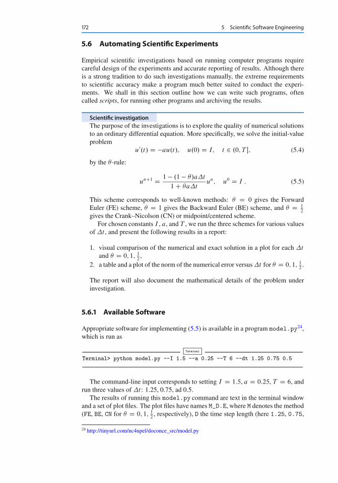
172 5 Scientific Software Engineering
5.6 Automating Scientific Experiments
Empirical scientific investigations based on running computer programs requirecareful design of the experiments and accurate reporting of results. Although thereis a strong tradition to do such investigations manually, the extreme requirementsto scientific accuracy make a program much better suited to conduct the experi-ments. We shall in this section outline how we can write such programs, oftencalled scripts, for running other programs and archiving the results.
Scientific investigationThe purpose of the investigations is to explore the quality of numerical solutionsto an ordinary differential equation. More specifically, we solve the initial-valueproblem
u0.t/ D �au.t/; u.0/ D I; t 2 .0; T �; (5.4)
by the �-rule:
unC1 D 1 � .1 � �/a�t
1C �a�tun; u0 D I : (5.5)
This scheme corresponds to well-known methods: � D 0 gives the ForwardEuler (FE) scheme, � D 1 gives the Backward Euler (BE) scheme, and � D 1
2
gives the Crank–Nicolson (CN) or midpoint/centered scheme.For chosen constants I , a, and T , we run the three schemes for various values
of �t , and present the following results in a report:
1. visual comparison of the numerical and exact solution in a plot for each �t
and � D 0; 1; 12,
2. a table and a plot of the norm of the numerical error versus �t for � D 0; 1; 12.
The report will also document the mathematical details of the problem underinvestigation.
5.6.1 Available Software
Appropriate software for implementing (5.5) is available in a program model.py24,which is run as
Terminal
Terminal> python model.py --I 1.5 --a 0.25 --T 6 --dt 1.25 0.75 0.5
The command-line input corresponds to setting I D 1:5, a D 0:25, T D 6, andrun three values of �t : 1.25, 0.75, ad 0.5.
The results of running this model.py command are text in the terminal windowand a set of plot files. The plot files have names M_D.E, where M denotes the method(FE, BE, CN for � D 0; 1; 1
2, respectively), D the time step length (here 1.25, 0.75,
24 http://tinyurl.com/nc4upel/doconce_src/model.py

5.6 Automating Scientific Experiments 173
or 0.5), and E is the plot file extension png or pdf. The text output in the terminalwindow looks like
0.0 1.25: 5.998E-010.0 0.75: 1.926E-010.0 0.50: 1.123E-010.0 0.10: 1.558E-020.5 1.25: 6.231E-020.5 0.75: 1.543E-020.5 0.50: 7.237E-030.5 0.10: 2.469E-041.0 1.25: 1.766E-011.0 0.75: 8.579E-021.0 0.50: 6.884E-021.0 0.10: 1.411E-02
The first column is the � value, the next the �t value, and the final column repre-sents the numerical error E (the norm of discrete error function on the mesh).
5.6.2 The Results WeWant to Produce
The results we need for our investigations are slightly different than what is directlyproduced by model.py:
1. We need to collect all the plots for one numerical method (FE, BE, CN) ina single plot. For example, if 4 �t values are run, the summarizing figure forthe BE method has 2 2 subplots, with the subplot corresponding to the largest�t in the upper left corner and the smallest in the bottom right corner.
2. We need to create a table containing �t values in the first column and the nu-merical error E for � D 0; 0:5; 1 in the next three columns. This table shouldbe available as a standard CSV file.
3. We need to plot the numerical error E versus �t in a log-log plot.
Consequently, we must write a script that can run model.py as described and pro-duce the results 1–3 above. This requires combining multiple plot files into one fileand interpreting the output from model.py as data for plotting and file storage.
If the script’s name is exper1.py, we run it with the desired �t values as posi-tional command-line arguments:
Terminal
Terminal> python exper1.py 0.5 0.25 0.1 0.05
This run will then generate eight plot files: FE.png and FE.pdf summarizingthe plots with the FE method, BE.png and BE.pdf with the BE method, CN.pngand CN.pdf with the CN method, and error.png and error.pdfwith the log-logplot of the numerical error versus �t . In addition, the table with numerical errors iswritten to a file error.csv.
Reproducible and replicable scienceA script that automates running our computer experiments will ensure that theexperiments can easily be rerun by anyone in the future, either to confirm the

174 5 Scientific Software Engineering
same results or redo the experiments with other input data. Also, whatever wedid to produce the results is documented in every detail in the script.
A project where anyone can easily repeat the experiments with the samedata is referred to as being replicable, and replicability should be a fundamentalrequirement in scientific computing work. Of more scientific interest is repro-ducibilty, which means that we can also run alternative experiments to arrive atthe same conclusions. This requires more than an automating script.
5.6.3 Combining Plot Files
The script for running experiments needs to combine multiple image files into one.The montage25 and convert26 programs in the ImageMagick software suite canbe used to combine image files. However, these programs are best suited for PNGfiles. For vector plots in PDF format one needs other tools to preserve the quality:pdftk, pdfnup, and pdfcrop.
Suppose you have four files f1.png, f2.png, f3.png, and f4.png and want tocombine them into a 2 2 table of subplots in a new file f.png, see Fig. 5.4 for anexample.
Fig. 5.4 Illustration of the Backward Euler method for four time step values
25 http://www.imagemagick.org/script/montage.php26 http://www.imagemagick.org/script/convert.php

5.6 Automating Scientific Experiments 175
The appropriate ImageMagick commands are
Terminal
Terminal> montage -background white -geometry 100% -tile 2x \f1.png f2.png f3.png f4.png f.png
Terminal> convert -trim f.png f.pngTerminal> convert f.png -transparent white f.png
The first command mounts the four files in one, the next convert commandremoves unnecessary surrounding white space, and the final convert commandmakes the white background transparent.
High-quality montage of PDF files f1.pdf, f2.pdf, f3.pdf, and f4.pdf intof.pdf goes like
Terminal
Terminal> pdftk f1.pdf f2.pdf f3.pdf f4.pdf output tmp.pdfTerminal> pdfnup --nup 2x2 --outfile tmp.pdf tmp.pdfTerminal> pdfcrop tmp.pdf f.pdfTerminal> rm -f tmp.pdf
5.6.4 Running a Program from Python
The script for automating experiments needs to run the model.py program withappropriate command-line options. Python has several tools for executing an arbi-trary command in the operating systems. Let cmd be a string containing the desiredcommand. In the present case study, cmd could be ’python model.py –I 1 –dt0.5 0.2’. The following code executes cmd and loads the text output into a stringoutput:
from subprocess import Popen, PIPE, STDOUTp = Popen(cmd, shell=True, stdout=PIPE, stderr=STDOUT)output, _ = p.communicate()
# Check if the execution was successfulfailure = p.returncodeif failure:
print ’Command failed:’, cmd; sys.exit(1)
Unsuccessful execution usually makes it meaningless to continue the program, andtherefore we abort the program with sys.exit(1). Any argument different from 0signifies to the computer’s operating system that our program stopped with a failure.
Programming tip: use _ for dummy variableSometimes we need to unpack tuples or lists in separate variables, but we are notinterested in all the variables. One example is
output, error = p.communicate()

176 5 Scientific Software Engineering
but error is of no interest in the example above. One can then use underscore _as variable name for the dummy (uninteresting) variable(s):
output, _ = p.communicate()
Here is another example where we iterate over a list of three-tuples, but theinterest is limited to the second element in each three-tuple:
for _, value, _ in list_of_three_tuples:# work with value
We need to interpret the contents of the string output and store the data inan appropriate data structure for further processing. Since the content is basicallya table and will be transformed to a spread sheet format, we let the columns inthe table be represented by lists in the program, and we collect these columns ina dictionary whose keys are natural column names: dt and the three values of � .The following code translates the output of cmd (output) to such a dictionary oflists (errors):
errors = {’dt’: dt_values, 1: [], 0: [], 0.5: []}for line in output.splitlines():
words = line.split()if words[0] in (’0.0’, ’0.5’, ’1.0’): # line with E?
# typical line: 0.0 1.25: 7.463E+00theta = float(words[0])E = float(words[2])errors[theta].append(E)
5.6.5 The Automating Script
We have now all the core elements in place to write the complete script where werun model.py for a set of �t values (given as positional command-line arguments),make the error plot, write the CSV file, and combine plot files as described above.The complete code is listed below, followed by some explaining comments.
import os, sys, globimport matplotlib.pyplot as plt
def run_experiments(I=1, a=2, T=5):# The command line must contain dt valuesif len(sys.argv) > 1:
dt_values = [float(arg) for arg in sys.argv[1:]]else:
print ’Usage: %s dt1 dt2 dt3 ...’ % sys.argv[0]sys.exit(1) # abort
# Run module file and grab outputcmd = ’python model.py --I %g --a %g --T %g’ % (I, a, T)dt_values_str = ’ ’.join([str(v) for v in dt_values])cmd += ’ --dt %s’ % dt_values_strprint cmd

5.6 Automating Scientific Experiments 177
from subprocess import Popen, PIPE, STDOUTp = Popen(cmd, shell=True, stdout=PIPE, stderr=STDOUT)output, _ = p.communicate()failure = p.returncodeif failure:
print ’Command failed:’, cmd; sys.exit(1)
errors = {’dt’: dt_values, 1: [], 0: [], 0.5: []}for line in output.splitlines():
words = line.split()if words[0] in (’0.0’, ’0.5’, ’1.0’): # line with E?
# typical line: 0.0 1.25: 7.463E+00theta = float(words[0])E = float(words[2])errors[theta].append(E)
# Find min/max for the axisE_min = 1E+20; E_max = -E_minfor theta in 0, 0.5, 1:
E_min = min(E_min, min(errors[theta]))E_max = max(E_max, max(errors[theta]))
plt.loglog(errors[’dt’], errors[0], ’ro-’)plt.loglog(errors[’dt’], errors[0.5], ’b+-’)plt.loglog(errors[’dt’], errors[1], ’gx-’)plt.legend([’FE’, ’CN’, ’BE’], loc=’upper left’)plt.xlabel(’log(time step)’)plt.ylabel(’log(error)’)plt.axis([min(dt_values), max(dt_values), E_min, E_max])plt.title(’Error vs time step’)plt.savefig(’error.png’); plt.savefig(’error.pdf’)
# Write out a table in CSV formatf = open(’error.csv’, ’w’)f.write(r’$\Delta t$,$\theta=0$,$\theta=0.5$,$\theta=1$’ \
+ ’\n’)for _dt, _fe, _cn, _be in zip(
errors[’dt’], errors[0], errors[0.5], errors[1]):f.write(’%.2f,%.4f,%.4f,%.4f\n’ % \
(_dt, _fe, _cn, _be))f.close()
# Combine images into rows with 2 plots in each rowimage_commands = []for method in ’BE’, ’CN’, ’FE’:
pdf_files = ’ ’.join([’%s_%g.pdf’ % (method, dt)for dt in dt_values])
png_files = ’ ’.join([’%s_%g.png’ % (method, dt)for dt in dt_values])
image_commands.append(’montage -background white -geometry 100%’ +’ -tile 2x %s %s.png’ % (png_files, method))
image_commands.append(’convert -trim %s.png %s.png’ % (method, method))
image_commands.append(’convert %s.png -transparent white %s.png’ %(method, method))
image_commands.append(’pdftk %s output tmp.pdf’ % pdf_files)
num_rows = int(round(len(dt_values)/2.0))image_commands.append(
’pdfnup --nup 2x%d --outfile tmp.pdf tmp.pdf’ % \num_rows)
image_commands.append(’pdfcrop tmp.pdf %s.pdf’ % method)

178 5 Scientific Software Engineering
for cmd in image_commands:print cmdfailure = os.system(cmd)if failure:
print ’Command failed:’, cmd; sys.exit(1)
# Remove the files generated above and by model.pyfrom glob import globfilenames = glob(’*_*.png’) + glob(’*_*.pdf’) + \
glob(’tmp*.pdf’)for filename in filenames:
os.remove(filename)
if __name__ == ’__main__’:run_experiments(I=1, a=2, T=5)plt.show()
We may comment upon many useful constructs in this script:
� [float(arg) for arg in sys.argv[1:]] builds a list of real numbersfrom all the command-line arguments.
� [’%s_%s.png’ % (method, dt) for dt in dt_values] builds a list offilenames from a list of numbers (dt_values).
� All montage, convert, pdftk, pdfnup, and pdfcrop commands for creatingcomposite figures are stored in a list and later executed in a loop.
� glob(’*_*.png’) returns a list of the names of all files in the current directorywhere the filename matches the Unix wildcard notation27 *_*.png (meaningany text, underscore, any text, and then .png).
� os.remove(filename) removes the file with name filename.� failure = os.system(cmd) runs an operating system command with simpler
syntax than what is required by subprocess (but the output of cmd cannot becaptured).
5.6.6 Making a Report
The results of running computer experiments are best documented in a little reportcontaining the problem to be solved, key code segments, and the plots from a seriesof experiments. At least the part of the report containing the plots should be auto-matically generated by the script that performs the set of experiments, because inthe script we know exactly which input data that were used to generate a specificplot, thereby ensuring that each figure is connected to the right data. Take a look ata sample report28 to see what we have in mind.
Word, OpenOffice, GoogleDocs Microsoft Word, its open source counterpartsOpenOffice and LibreOffice, along with GoogleDocs and similar online servicesare the dominating tools for writing reports today. Nevertheless, scientific reportsoften need mathematical equations and nicely typeset computer code in monospacefont. The support for mathematics and computer code in the mentioned tools is
27 http://en.wikipedia.org/wiki/Glob_(programming)28 http://tinyurl.com/nc4upel/_static/sphinx-cloud/

5.6 Automating Scientific Experiments 179
Fig. 5.5 Report in HTML format with MathJax
in this author’s view not on par with the technologies based on markup languagesand which are addressed below. Also, with markup languages one has a readable,pure text file as source for the report, and changes in this text can easily be trackedby version control systems like Git. The result is a very strong tool for monitor-ing “who did what when” with the files, resulting in increased reliability of thewriting process. For collaborative writing, the merge functionality in Git leads tosafer simultaneously editing than what is offered even by collaborative tools likeGoogleDocs.
HTML with MathJax HTML is the markup language used for web pages. Nicelytypeset computer code is straightforward in HTML, and high-quality mathematicaltypesetting is available using an extension to HTML called MathJax29, which allowsformulas and equations to be typeset with LATEX syntax and nicely rendered in webbrowsers, see Fig. 5.5. A relatively small subset of LATEX environments for mathe-matics is supported, but the syntax for formulas is quite rich. Inline formulas looklike \( u’=-au \) while equations are surrounded by $$ signs. Inside such signs,one can use \[ u’=-au \] for unnumbered equations, or \begin{equation} and\end{equation} for numbered equations, or \begin{align} and \end{align}for multiple numbered aligned equations. You need to be familiar with mathemati-cal typesetting in LaTeX30 to write MathJax code.
29 http://www.mathjax.org/30 http://en.wikibooks.org/wiki/LaTeX/Mathematics

180 5 Scientific Software Engineering
Fig. 5.6 Report in PDF format generated from LATEX source
The file exper1_mathjax.py31 calls a script exper1.py32 to perform the nu-merical experiments and then runs Python statements for creating an HTML file33
with the source code for the scientific report34.
LATEX The de facto language for mathematical typesetting and scientific reportwriting is LaTeX35. A number of very sophisticated packages have been added tothe language over a period of three decades, allowing very fine-tuned layout andtypesetting. For output in the PDF format36, see Fig. 5.6 for an example, LATEXis the definite choice when it comes to typesetting quality. The LATEX languageused to write the reports has typically a lot of commands involving backslashesand braces37, and many claim that LATEX syntax is not particularly readable. Foroutput on the web via HTML code (i.e., not only showing the PDF in the browserwindow), LATEX struggles with delivering high quality typesetting. Other tools, es-pecially Sphinx, give better results and can also produce nice-looking PDFs. Thefile exper1_latex.py38 shows how to generate the LATEX source from a program.
Sphinx Sphinx39 is a typesetting language with similarities to HTML and LATEX,but with much less tagging. It has recently become very popular for software doc-umentation and mathematical reports. Sphinx can utilize LATEX for mathematical
31 http://tinyurl.com/p96acy2/report_generation/exper1_html.py32 http://tinyurl.com/p96acy2/exper1.py33 http://tinyurl.com/nc4upel/_static/report_mathjax.html.html34 http://tinyurl.com/nc4upel/_static/report_mathjax.html35 http://en.wikipedia.org/wiki/LaTeX36 http://tinyurl.com/nc4upel/_static/report.pdf37 http://tinyurl.com/nc4upel/_static/report.tex.html38 http://tinyurl.com/p96acy2/report_generation/exper1_latex.py39 http://sphinx.pocoo.org/

5.6 Automating Scientific Experiments 181
Fig. 5.7 Report in HTML format generated from Sphinx source
formulas and equations. Unfortunately, the subset of LATEX mathematics supportedis less than in full MathJax (in particular, numbering of multiple equations in analign type environment is not supported). The Sphinx syntax40 is an extension ofthe reStructuredText language. An attractive feature of Sphinx is its rich supportfor fancy layout of web pages41. In particular, Sphinx can easily be combined withvarious layout themes that give a certain look and feel to the web site and that offerstable of contents, navigation, and search facilities, see Fig. 5.7.
Markdown A recent, very popular format for easy writing of web pages is Mark-down42. Text is written very much like one would do in email, using spacingand special characters to naturally format the code instead of heavily tagging thetext as in LATEX and HTML. With the tool Pandoc43 one can go from Markdownto a variety of formats. HTML is a common output format, but LATEX, epub,XML, OpenOffice/LibreOffice, MediaWiki, and Microsoft Word are some otherpossibilities. A Markdown version of our scientific report demo is available as anIPython/Jupyter notebook (described next).
IPython/Jupyter notebooks. The Jupyter Notebook44 is a web-based tool whereone can write scientific reports with live computer code and graphics. Or the otherway around: software can be equipped with documentation in the style of scien-tific reports. A slightly extended version of Markdown is used for writing text andmathematics, and the source code of a notebook45 is in json format. The interest in
40 http://tinyurl.com/nc4upel/_static/report_sphinx.rst.html41 http://tinyurl.com/nc4upel/_static/sphinx-cloud/index.html42 http://daringfireball.net/projects/markdown/43 http://johnmacfarlane.net/pandoc/44 http://jupyter.org45 http://tinyurl.com/nc4upel/_static/report.ipynb.html
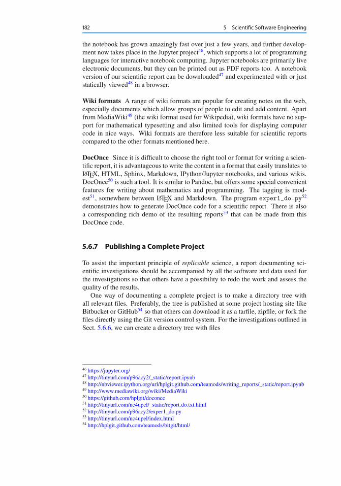
182 5 Scientific Software Engineering
the notebook has grown amazingly fast over just a few years, and further develop-ment now takes place in the Jupyter project46, which supports a lot of programminglanguages for interactive notebook computing. Jupyter notebooks are primarily liveelectronic documents, but they can be printed out as PDF reports too. A notebookversion of our scientific report can be downloaded47 and experimented with or juststatically viewed48 in a browser.
Wiki formats A range of wiki formats are popular for creating notes on the web,especially documents which allow groups of people to edit and add content. Apartfrom MediaWiki49 (the wiki format used for Wikipedia), wiki formats have no sup-port for mathematical typesetting and also limited tools for displaying computercode in nice ways. Wiki formats are therefore less suitable for scientific reportscompared to the other formats mentioned here.
DocOnce Since it is difficult to choose the right tool or format for writing a scien-tific report, it is advantageous to write the content in a format that easily translates toLATEX, HTML, Sphinx, Markdown, IPython/Jupyter notebooks, and various wikis.DocOnce50 is such a tool. It is similar to Pandoc, but offers some special convenientfeatures for writing about mathematics and programming. The tagging is mod-est51, somewhere between LATEX and Markdown. The program exper1_do.py52
demonstrates how to generate DocOnce code for a scientific report. There is alsoa corresponding rich demo of the resulting reports53 that can be made from thisDocOnce code.
5.6.7 Publishing a Complete Project
To assist the important principle of replicable science, a report documenting sci-entific investigations should be accompanied by all the software and data used forthe investigations so that others have a possibility to redo the work and assess thequality of the results.
One way of documenting a complete project is to make a directory tree withall relevant files. Preferably, the tree is published at some project hosting site likeBitbucket or GitHub54 so that others can download it as a tarfile, zipfile, or fork thefiles directly using the Git version control system. For the investigations outlined inSect. 5.6.6, we can create a directory tree with files
46 https://jupyter.org/47 http://tinyurl.com/p96acy2/_static/report.ipynb48 http://nbviewer.ipython.org/url/hplgit.github.com/teamods/writing_reports/_static/report.ipynb49 http://www.mediawiki.org/wiki/MediaWiki50 https://github.com/hplgit/doconce51 http://tinyurl.com/nc4upel/_static/report.do.txt.html52 http://tinyurl.com/p96acy2/exper1_do.py53 http://tinyurl.com/nc4upel/index.html54 http://hplgit.github.com/teamods/bitgit/html/

5.7 Exercises 183
setup.py./src:
model.py./doc:
./src:exper1_mathjax.pymake_report.shrun.sh
./pub:report.html
The src directory holds source code (modules) to be reused in other projects,the setup.py script builds and installs such software, the doc directory containsthe documentation, with src for the source of the documentation (usually writ-ten in a markup language) and pub for published (compiled) documentation. Therun.sh file is a simple Bash script listing the python commands we used to runexper1_mathjax.py to generate the experiments and the report.html file.
5.7 Exercises
Problem 5.1: Make a tool for differentiating curvesSuppose we have a curve specified through a set of discrete coordinates .xi ; yi /,i D 0; : : : ; n, where the xi values are uniformly distributed with spacing �x: xi D�x. The derivative of this curve, defined as a new curve with points .xi ; di /, canbe computed via finite differences:
d0 D y1 � y0
�x; (5.6)
di D yiC1 � yi�1
2�x; i D 1; : : : ; n � 1; (5.7)
dn D yn � yn�1
�x: (5.8)
a) Write a function differentiate(x, y) for differentiating a curve with coor-dinates in the arrays x and y, using the formulas above. The function shouldreturn the coordinate arrays of the resulting differentiated curve.
b) Since the formulas for differentiation used here are only approximate, with un-known approximation errors, it is challenging to construct test cases. Here arethree approaches, which should be implemented in three separate test functions.1. Consider a curve with three points and compute di , i D 0; 1; 2, by hand.
Make a test that compares the hand-calculated results with those from thefunction in a).
2. The formulas for di are exact for points on a straight line, as all the di val-ues are then the same, equal to the slope of the line. A test can check thisproperty.
3. For points lying on a parabola, the values for di , i D 1; : : : ; n � 1, shouldequal the exact derivative of the parabola. Make a test based on this property.
c) Start with a curve corresponding to y D sin.x/ and n C 1 points in Œ0; 1�.Apply differentiate four times and plot the resulting curve and the exacty D sin x for n D 6; 11; 21; 41.
Filename: curvediff.

184 5 Scientific Software Engineering
Problem 5.2: Make solid software for the Trapezoidal ruleAn integral
bZa
f .x/dx
can be numerically approximated by the Trapezoidal rule,
bZa
f .x/dx � h
2.f .a/C f .b//C h
n�1XiD1
f .xi /;
where xi is a set of uniformly spaced points in Œa; b�:
h D b � a
n; xi D aC ih; i D 1; : : : ; n � 1 :
Somebody has used this rule to compute the integralR
0sin2 x dx:
from math import pi, sinnp = 20h = pi/npI = 0for k in range(1, np):
I += sin(k*h)**2print I
a) The “flat” implementation above suffers from serious flaws:1. A general numerical algorithm (the Trapezoidal rule) is implemented in
a specialized form where the formula for f is inserted directly into the codefor the general integration formula.
2. A general numerical algorithm is not encapsulated as a general function,with appropriate parameters, which can be reused across a wide range ofapplications.
3. The lazy programmer dropped the first terms in the general formula sincesin.0/ D sin./ D 0.
4. The sloppy programmer used np (number of points?) as variable for n inthe formula and a counter k instead of i. Such small deviations from themathematical notation are completely unnecessary. The closer the code andthe mathematics can get, the easier it is to spot errors in formulas.
Write a function trapezoidal that fixes these flaws. Place the function ina module trapezoidal.
b) Write a test function test_trapezoidal. Call the test function explicitly tocheck that it works. Remove the call and run pytest on the module:
Terminal
Terminal> py.test -s -v trapezoidal

5.7 Exercises 185
Hint Note that even if you know the value of the integral, you do not know the errorin the approximation produced by the Trapezoidal rule. However, the Trapezoidalrule will integrate linear functions exactly (i.e., to machine precision). Base a testfunction on a linear f .x/.
c) Add functionality such that we can computeR b
af .x/dx by providing f , a, b,
and n as positional command-line arguments to the module file:
Terminal
Terminal> python trapezoidal.py ’sin(x)**2’ 0 pi 20
Here, a D 0, b D , and n D 20.Note that the trapezoidal.py file must still be a valid module file, so theinterpretation of command-line data and computation of the integral must beperformed from calls in a test block.
Hint To translate a string formula on the command line, like sin(x)**2, intoa Python function, you can wrap a function declaration around the formula andrun exec on the string to turn it into live Python code:
import math, sysformula = sys.argv[1]f_code = """def f(x):
return %s""" % formulaexec(code, math.__dict__)
The result is the same as if we had hardcoded
from math import *
def f(x):return sin(x)**2
in the program. Note that exec needs the namespace math.__dict__, i.e., allnames in the math module, such that it understands sin and other mathematicalfunctions. Similarly, to allow a and b to be math expressions like pi/4 and exp(4),do
Terminal
a = eval(sys.argv[2], math.__dict__)b = eval(sys.argv[2], math.__dict__)
d) Write a test function for verifying the implementation of data reading from thecommand line.
Filename: trapezoidal.
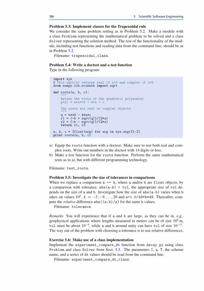
186 5 Scientific Software Engineering
Problem 5.3: Implement classes for the Trapezoidal ruleWe consider the same problem setting as in Problem 5.2. Make a module witha class Problem representing the mathematical problem to be solved and a classSolver representing the solution method. The rest of the functionality of the mod-ule, including test functions and reading data from the command line, should be asin Problem 5.2.
Filename: trapezoidal_class.
Problem 5.4: Write a doctest and a test functionType in the following program:
import sys# This sqrt(x) returns real if x>0 and complex if x<0from numpy.lib.scimath import sqrt
def roots(a, b, c):"""Return the roots of the quadratic polynomialp(x) = a*x**2 + b*x + c.
The roots are real or complex objects."""q = b**2 - 4*a*cr1 = (-b + sqrt(q))/(2*a)r2 = (-b - sqrt(q))/(2*a)return r1, r2
a, b, c = [float(arg) for arg in sys.argv[1:]]print roots(a, b, c)
a) Equip the roots function with a doctest. Make sure to test both real and com-plex roots. Write out numbers in the doctest with 14 digits or less.
b) Make a test function for the roots function. Perform the same mathematicaltests as in a), but with different programming technology.
Filename: test_roots.
Problem 5.5: Investigate the size of tolerances in comparisonsWhen we replace a comparison a == b, where a and/or b are float objects, bya comparison with tolerance, abs(a-b) < tol, the appropriate size of tol de-pends on the size of a and b. Investigate how the size of abs(a-b) varies when btakes on values 10k , k D �5;�9; : : : ; 20 and a=1.0/49*b*49. Thereafter, com-pute the relative difference abs((a-b)/a) for the same b values.
Filename: tolerance.
Remarks You will experience that if a and b are large, as they can be in, e.g.,geophysical applications where lengths measured in meters can be of size 106 m,tol must be about 10�9, while a and b around unity can have tol of size 10�15.The way out of the problem with choosing a tolerance is to use relative differences.
Exercise 5.6: Make use of a class implementationImplement the experiment_compare_dt function from decay.py using classProblem and class Solver from Sect. 5.5. The parameters I, a, T, the schemename, and a series of dt values should be read from the command line.
Filename: experiment_compare_dt_class.

5.7 Exercises 187
Problem 5.7: Make solid software for a difference equationWe have the following evolutionary difference equation for the number of individ-uals un of a certain specie at time n�t :
unC1 D un C�t run
�1 � un
M n
�; u0 D U0 : (5.9)
Here, n is a counter in time, �t is time between time levels n and nC 1 (assumedconstant), r is a net reproduction rate for the specie, and M n is the upper limit ofthe population that the environment can sustain at time level n.
Filename: logistic.
Open Access This chapter is distributed under the terms of the Creative Commons Attribution-NonCommercial 4.0 International License (http://creativecommons.org/licenses/by-nc/4.0/),which permits any noncommercial use, duplication, adaptation, distribution and reproductionin any medium or format, as long as you give appropriate credit to the original author(s) and thesource, a link is provided to the Creative Commons license and any changes made are indicated.
The images or other third party material in this chapter are included in the work’s CreativeCommons license, unless indicated otherwise in the credit line; if such material is not includedin the work’s Creative Commons license and the respective action is not permitted by statutoryregulation, users will need to obtain permission from the license holder to duplicate, adapt orreproduce the material.

References
1. W. Gander, M. J. Gander, and F. Kwok, Scientific Computing - An Introducting Using Mapleand MATLAB. Texts in Computational Science and Engineering. Springer, 2015
2. D. Griffiths, F. David, and D. J. Higham, Numerical Methods for Ordinary Differential Equa-tions: Initial Value Problems. Springer, 2010
3. E. Hairer, S. P. Nørsett, and G. Wanner, Solving Ordinary Differential Equations I. NonstiffProblems. Springer, 1993
4. G. Hairer and E. Wanner, Solving Ordinary Differential Equations II. Springer, 2010
5. J. D. Hunter, D. Dale, E. Firing, and M. Droettboom, Matplotlib documentation, 2012. http://matplotlib.org/users/
6. H. P. Langtangen, Quick intro to version control systems and project hosting sites. http://hplgit.github.io/teamods/bitgit/html/
7. H. P. Langtangen, SciTools documentation. http://hplgit.github.io/scitools/doc/web/index.html
8. H. P. Langtangen, A Primer on Scientific Programming with Python. Texts in ComputationalScience and Engineering. Springer, fourth edition, 2014
9. H. P. Langtangen and G. K. Pedersen, Scaling of Differential Equations. SimulaSpringerBrief.Springer, 2015. http://tinyurl.com/qfjgxmf/web
10. H. P. Langtangen and L. Wang, Odespy software package. https://github.com/hplgit/odespy
11. D. B. Meade and A. A. Struthers, Differential equations in the new millenium: the parachuteproblem. International Journal of Engineering Education, 15(6):417–424, 1999
12. L. Petzold and U. M. Ascher, Computer Methods for Ordinary Differential Equations andDifferential-Algebraic Equations, volume 61. SIAM, 1998
13. L. N. Trefethen, Trefethen’s index cards - Forty years of notes about People, Words andMathematics. World Scientific, 2011
189© The Author(s) 2016H.P. Langtangen, Finite Difference Computing with Exponential Decay Models,Lecture Notes in Computational Science and Engineering 110,DOI 10.1007/978-3-319-29439-1

Index
�-rule, 10, 77
AAdams–Bashforth scheme, 2nd-order, 79Adams–Bashforth scheme, 3rd order, 79adaptive time stepping, 85algebraic equation, 5amplification factor, 45argparse (Python module), 146ArgumentParser (Python class), 146array arithmetics, 25, 35array computing, 25, 35A-stable methods, 45averaging
arithmetic, 9geometric, 108
Bbackward difference, 7Backward Euler scheme, 7backward scheme, 1-step, 7backward scheme, 2-step, 77BDF2 scheme, 77
Ccentered difference, 8chemical reactions
irreversible, 98reversible, 99
command-line arguments, 145, 146consistency, 53continuous function norms, 26convergence, 53convergence rate, 73Crank–Nicolson scheme, 8cropping images, 30
Ddebugging, 138decay ODE, 1
difference equation, 5directory, 15discrete equation, 5discrete function norms, 26Distutils, 163doc strings, 18DocOnce, 182doctest in test function, 156doctests, 151Dormand-Prince Runge–Kutta 4-5 method, 85
EEPS plot, 29error
amplification factor, 49global, 50norms, 28
explicit schemes, 77exponential decay, 1
Ffinite difference operator notation, 14finite difference scheme, 5finite differences, 4
backward, 7centered, 8forward, 4
folder, 15format string syntax (Python), 20forward difference, 4Forward Euler scheme, 5
Ggeometric mean, 108GitHub, 163Google Docs, 178grid, 2
HHeun’s method, 78
191
192 Index
HTML, 179
Iimplicit schemes, 77importing modules, 131, 165interactive Python, 47IPython notebooks, 181isympy, 47
JJupyter notebooks, 181
KKelvin–Voigt material model, 110
Llambda functions, 70LaTeX, 180Leapfrog scheme, 78Leapfrog scheme, filtered, 78LibreOffice, 178list comprehension, 145logger, 138logging module, 138logistic model, 94Lotka-Volterra model, 102L-stable methods, 45
MMarkdown, 181MathJax, 179mesh, 2mesh function, 3mesh function norms, 26method of manufactured solutions, 71MMS (method of manufactured solutions), 71montage program, 30Monte Carlo simulation, 58
Nnorm
continuous, 26discrete (mesh function), 26
nose tests, 153
Oode45, 85OpenOffice, 178operator notation, finite differences, 14option-value pairs (command line), 146os.system, 176
PPDF plot, 29pdfcrop program, 31pdfnup program, 31pdftk program, 31plotting curves, 21PNG plot, 29
population dynamics, 93predator-prey model, 102printf format, 19problem class, 167pytest tests, 153
Rradioactive decay, 95reading the command line, 146refactoring, 130relative differences, 154, 186replicability, 173, 182representative (mesh function), 25reproducibility, 173RK4, 80Runge–Kutta, 2nd-order method, 78Runge–Kutta, 4th-order method, 80
Sscalar computing, 28scaling, 109setup.py, 162software testing
doctests, 151nose, 153pytest, 153test function, 153unit testing (class-based), 160
solver class, 168Sphinx (typesetting tool), 180stability, 45, 53sympy, 47sys.argv, 145
TTaylor-series methods (for ODEs), 79terminal velocity, 108test function, 24, 153TestCase (class in unittest), 160theta-rule, 10, 77time step, 11
Uunit testing, 24, 153, 160unittest, 160Unix wildcard notation, 176
Vvectorization, 25, 35verification, 75viewing graphics files, 29viscoelasticity, 110visualizing curves, 21
Wweighted average, 10wildcard notation (Unix), 176Word (Microsoft), 178wrapper (code), 168

Editorial Policy
1. Volumes in the following three categories will be published in LNCSE:
i) Research monographsii) Tutorialsiii) Conference proceedings
Those considering a book which might be suitable for the series are strongly advised tocontact the publisher or the series editors at an early stage.
2. Categories i) and ii). Tutorials are lecture notes typically arising via summer schoolsor similar events, which are used to teach graduate students. These categories will beemphasized by Lecture Notes in Computational Science and Engineering. Submissions byinterdisciplinary teams of authors are encouraged. The goal is to report new develop-ments – quickly, informally, and in a way that will make them accessible to non-specialists.In the evaluation of submissions timeliness of the work is an important criterion. Textsshould be well-rounded, well-written and reasonably self-contained. In most cases the workwill contain results of others as well as those of the author(s). In each case the author(s)should provide sufficient motivation, examples, and applications. In this respect, Ph.D. theseswill usually be deemed unsuitable for the Lecture Notes series. Proposals for volumes inthese categories should be submitted either to one of the series editors or to Springer-Verlag,Heidelberg, and will be refereed. A provisional judgement on the acceptability of a projectcan be based on partial information about the work: a detailed outline describing the contentsof each chapter, the estimated length, a bibliography, and one or two sample chapters – ora first draft. A final decision whether to accept will rest on an evaluation of the completedwork which should include
– at least 100 pages of text;– a table of contents;– an informative introduction perhaps with some historical remarks which should be acces-
sible to readers unfamiliar with the topic treated;– a subject index.
3. Category iii). Conference proceedings will be considered for publication provided thatthey are both of exceptional interest and devoted to a single topic. One (or more) expertparticipants will act as the scientific editor(s) of the volume. They select the papers which aresuitable for inclusion and have them individually refereed as for a journal. Papers not closelyrelated to the central topic are to be excluded. Organizers should contact the Editor for CSEat Springer at the planning stage, see Addresses below.
In exceptional cases some other multi-author-volumes may be considered in this category.
4. Only works in English will be considered. For evaluation purposes, manuscripts maybe submitted in print or electronic form, in the latter case, preferably as pdf- or zippedps-files. Authors are requested to use the LaTeX style files available from Springer athttp://www.springer.com/gp/authors-editors/book-authors-editors/manuscript-preparation/5636 (Click on LaTeX Template! monographs or contributed books).
For categories ii) and iii) we strongly recommend that all contributions in a volume be writtenin the same LaTeX version, preferably LaTeX2e. Electronic material can be included ifappropriate. Please contact the publisher.
Careful preparation of the manuscripts will help keep production time short besides ensuringsatisfactory appearance of the finished book in print and online.
5. The following terms and conditions hold. Categories i), ii) and iii):
Authors receive 50 free copies of their book. No royalty is paid.Volume editors receive a total of 50 free copies of their volume to be shared with authors, butno royalties.
Authors and volume editors are entitled to a discount of 33.3 % on the price of Springer bookspurchased for their personal use, if ordering directly from Springer.
6. Springer secures the copyright for each volume.
Addresses:
Timothy J. BarthNASA Ames Research CenterNAS DivisionMoffett Field, CA 94035, [email protected]
Michael GriebelInstitut für Numerische Simulationder Universität BonnWegelerstr. 653115 Bonn, [email protected]
David E. KeyesMathematical and Computer Sciencesand EngineeringKing Abdullah University of Scienceand TechnologyP.O. Box 55455Jeddah 21534, Saudi [email protected]
and
Department of Applied Physicsand Applied MathematicsColumbia University500 W. 120 th StreetNew York, NY 10027, [email protected]
Risto M. NieminenDepartment of Applied PhysicsAalto University School of Scienceand Technology00076 Aalto, [email protected]
Dirk RooseDepartment of Computer ScienceKatholieke Universiteit LeuvenCelestijnenlaan 200A3001 Leuven-Heverlee, [email protected]
Tamar SchlickDepartment of Chemistryand Courant Instituteof Mathematical SciencesNew York University251 Mercer StreetNew York, NY 10012, [email protected]
Editor for Computational Scienceand Engineering at Springer:Martin PetersSpringer-VerlagMathematics Editorial IVTiergartenstrasse 1769121 Heidelberg, [email protected]

Lecture Notesin Computational Scienceand Engineering
1. D. Funaro, Spectral Elements for Transport-Dominated Equations.
2. H.P. Langtangen, Computational Partial Differential Equations. Numerical Methods and DiffpackProgramming.
3. W. Hackbusch, G. Wittum (eds.), Multigrid Methods V.
4. P. Deuflhard, J. Hermans, B. Leimkuhler, A.E. Mark, S. Reich, R.D. Skeel (eds.), ComputationalMolecular Dynamics: Challenges, Methods, Ideas.
5. D. Kröner, M. Ohlberger, C. Rohde (eds.), An Introduction to Recent Developments in Theory andNumerics for Conservation Laws.
6. S. Turek, Efficient Solvers for Incompressible Flow Problems. An Algorithmic and ComputationalApproach.
7. R. von Schwerin, Multi Body System SIMulation. Numerical Methods, Algorithms, and Software.
8. H.-J. Bungartz, F. Durst, C. Zenger (eds.), High Performance Scientific and Engineering Comput-ing.
9. T.J. Barth, H. Deconinck (eds.), High-Order Methods for Computational Physics.
10. H.P. Langtangen, A.M. Bruaset, E. Quak (eds.), Advances in Software Tools for Scientific Comput-ing.
11. B. Cockburn, G.E. Karniadakis, C.-W. Shu (eds.), Discontinuous Galerkin Methods. Theory, Com-putation and Applications.
12. U. van Rienen, Numerical Methods in Computational Electrodynamics. Linear Systems in PracticalApplications.
13. B. Engquist, L. Johnsson, M. Hammill, F. Short (eds.), Simulation and Visualization on the Grid.
14. E. Dick, K. Riemslagh, J. Vierendeels (eds.), Multigrid Methods VI.
15. A. Frommer, T. Lippert, B. Medeke, K. Schilling (eds.), Numerical Challenges in Lattice QuantumChromodynamics.
16. J. Lang, Adaptive Multilevel Solution of Nonlinear Parabolic PDE Systems. Theory, Algorithm,and Applications.
17. B.I. Wohlmuth, Discretization Methods and Iterative Solvers Based on Domain Decomposition.
18. U. van Rienen, M. Günther, D. Hecht (eds.), Scientific Computing in Electrical Engineering.
19. I. Babuška, P.G. Ciarlet, T. Miyoshi (eds.), Mathematical Modeling and Numerical Simulation inContinuum Mechanics.
20. T.J. Barth, T. Chan, R. Haimes (eds.), Multiscale and Multiresolution Methods. Theory andApplications.
21. M. Breuer, F. Durst, C. Zenger (eds.), High Performance Scientific and Engineering Computing.
22. K. Urban, Wavelets in Numerical Simulation. Problem Adapted Construction and Applications.
23. L.F. Pavarino, A. Toselli (eds.), Recent Developments in Domain Decomposition Methods.
24. T. Schlick, H.H. Gan (eds.), Computational Methods for Macromolecules: Challenges andApplications.

25. T.J. Barth, H. Deconinck (eds.), Error Estimation and Adaptive Discretization Methods inComputational Fluid Dynamics.
26. M. Griebel, M.A. Schweitzer (eds.), Meshfree Methods for Partial Differential Equations.
27. S. Müller, Adaptive Multiscale Schemes for Conservation Laws.
28. C. Carstensen, S. Funken, W. Hackbusch, R.H.W. Hoppe, P. Monk (eds.), ComputationalElectromagnetics.
29. M.A. Schweitzer, A Parallel Multilevel Partition of Unity Method for Elliptic Partial DifferentialEquations.
30. T. Biegler, O. Ghattas, M. Heinkenschloss, B. van Bloemen Waanders (eds.), Large-Scale PDE-Constrained Optimization.
31. M. Ainsworth, P. Davies, D. Duncan, P. Martin, B. Rynne (eds.), Topics in Computational WavePropagation. Direct and Inverse Problems.
32. H. Emmerich, B. Nestler, M. Schreckenberg (eds.), Interface and Transport Dynamics. Computa-tional Modelling.
33. H.P. Langtangen, A. Tveito (eds.), Advanced Topics in Computational Partial DifferentialEquations. Numerical Methods and Diffpack Programming.
34. V. John, Large Eddy Simulation of Turbulent Incompressible Flows. Analytical and NumericalResults for a Class of LES Models.
35. E. Bänsch (ed.), Challenges in Scientific Computing – CISC 2002.
36. B.N. Khoromskij, G. Wittum, Numerical Solution of Elliptic Differential Equations by Reductionto the Interface.
37. A. Iske, Multiresolution Methods in Scattered Data Modelling.
38. S.-I. Niculescu, K. Gu (eds.), Advances in Time-Delay Systems.
39. S. Attinger, P. Koumoutsakos (eds.), Multiscale Modelling and Simulation.
40. R. Kornhuber, R. Hoppe, J. Périaux, O. Pironneau, O. Wildlund, J. Xu (eds.), Domain Decomposi-tion Methods in Science and Engineering.
41. T. Plewa, T. Linde, V.G. Weirs (eds.), Adaptive Mesh Refinement – Theory and Applications.
42. A. Schmidt, K.G. Siebert, Design of Adaptive Finite Element Software. The Finite Element ToolboxALBERTA.
43. M. Griebel, M.A. Schweitzer (eds.), Meshfree Methods for Partial Differential Equations II.
44. B. Engquist, P. Lötstedt, O. Runborg (eds.), Multiscale Methods in Science and Engineering.
45. P. Benner, V. Mehrmann, D.C. Sorensen (eds.), Dimension Reduction of Large-Scale Systems.
46. D. Kressner, Numerical Methods for General and Structured Eigenvalue Problems.
47. A. Boriçi, A. Frommer, B. Joó, A. Kennedy, B. Pendleton (eds.), QCD and Numerical Analysis III.
48. F. Graziani (ed.), Computational Methods in Transport.
49. B. Leimkuhler, C. Chipot, R. Elber, A. Laaksonen, A. Mark, T. Schlick, C. Schütte, R. Skeel (eds.),New Algorithms for Macromolecular Simulation.
50. M. Bücker, G. Corliss, P. Hovland, U. Naumann, B. Norris (eds.), Automatic Differentiation: Ap-plications, Theory, and Implementations.
51. A.M. Bruaset, A. Tveito (eds.), Numerical Solution of Partial Differential Equations on ParallelComputers.
52. K.H. Hoffmann, A. Meyer (eds.), Parallel Algorithms and Cluster Computing.

53. H.-J. Bungartz, M. Schäfer (eds.), Fluid-Structure Interaction.
54. J. Behrens, Adaptive Atmospheric Modeling.
55. O. Widlund, D. Keyes (eds.), Domain Decomposition Methods in Science and Engineering XVI.
56. S. Kassinos, C. Langer, G. Iaccarino, P. Moin (eds.), Complex Effects in Large Eddy Simulations.
57. M. Griebel, M.A Schweitzer (eds.), Meshfree Methods for Partial Differential Equations III.
58. A.N. Gorban, B. Kégl, D.C. Wunsch, A. Zinovyev (eds.), Principal Manifolds for Data Visualiza-tion and Dimension Reduction.
59. H. Ammari (ed.), Modeling and Computations in Electromagnetics: A Volume Dedicated to Jean-Claude Nédélec.
60. U. Langer, M. Discacciati, D. Keyes, O. Widlund, W. Zulehner (eds.), Domain DecompositionMethods in Science and Engineering XVII.
61. T. Mathew, Domain Decomposition Methods for the Numerical Solution of Partial DifferentialEquations.
62. F. Graziani (ed.), Computational Methods in Transport: Verification and Validation.
63. M. Bebendorf, Hierarchical Matrices. A Means to Efficiently Solve Elliptic Boundary ValueProblems.
64. C.H. Bischof, H.M. Bücker, P. Hovland, U. Naumann, J. Utke (eds.), Advances in AutomaticDifferentiation.
65. M. Griebel, M.A. Schweitzer (eds.), Meshfree Methods for Partial Differential Equations IV.
66. B. Engquist, P. Lötstedt, O. Runborg (eds.), Multiscale Modeling and Simulation in Science.
67. I.H. Tuncer, Ü. Gülcat, D.R. Emerson, K. Matsuno (eds.), Parallel Computational Fluid Dynamics2007.
68. S. Yip, T. Diaz de la Rubia (eds.), Scientific Modeling and Simulations.
69. A. Hegarty, N. Kopteva, E. O’Riordan, M. Stynes (eds.), BAIL 2008 – Boundary and InteriorLayers.
70. M. Bercovier, M.J. Gander, R. Kornhuber, O. Widlund (eds.), Domain Decomposition Methods inScience and Engineering XVIII.
71. B. Koren, C. Vuik (eds.), Advanced Computational Methods in Science and Engineering.
72. M. Peters (ed.), Computational Fluid Dynamics for Sport Simulation.
73. H.-J. Bungartz, M. Mehl, M. Schäfer (eds.), Fluid Structure Interaction II – Modelling, Simulation,Optimization.
74. D. Tromeur-Dervout, G. Brenner, D.R. Emerson, J. Erhel (eds.), Parallel Computational FluidDynamics 2008.
75. A.N. Gorban, D. Roose (eds.), Coping with Complexity: Model Reduction and Data Analysis.
76. J.S. Hesthaven, E.M. Rønquist (eds.), Spectral and High Order Methods for Partial DifferentialEquations.
77. M. Holtz, Sparse Grid Quadrature in High Dimensions with Applications in Finance and Insur-ance.
78. Y. Huang, R. Kornhuber, O.Widlund, J. Xu (eds.), Domain Decomposition Methods in Science andEngineering XIX.
79. M. Griebel, M.A. Schweitzer (eds.), Meshfree Methods for Partial Differential Equations V.
80. P.H. Lauritzen, C. Jablonowski, M.A. Taylor, R.D. Nair (eds.), Numerical Techniques for GlobalAtmospheric Models.

81. C. Clavero, J.L. Gracia, F.J. Lisbona (eds.), BAIL 2010 – Boundary and Interior Layers, Computa-tional and Asymptotic Methods.
82. B. Engquist, O. Runborg, Y.R. Tsai (eds.), Numerical Analysis and Multiscale Computations.
83. I.G. Graham, T.Y. Hou, O. Lakkis, R. Scheichl (eds.), Numerical Analysis of Multiscale Problems.
84. A. Logg, K.-A. Mardal, G. Wells (eds.), Automated Solution of Differential Equations by the FiniteElement Method.
85. J. Blowey, M. Jensen (eds.), Frontiers in Numerical Analysis – Durham 2010.
86. O. Kolditz, U.-J. Gorke, H. Shao, W. Wang (eds.), Thermo-Hydro-Mechanical-Chemical Processesin Fractured Porous Media – Benchmarks and Examples.
87. S. Forth, P. Hovland, E. Phipps, J. Utke, A. Walther (eds.), Recent Advances in Algorithmic Differ-entiation.
88. J. Garcke, M. Griebel (eds.), Sparse Grids and Applications.
89. M. Griebel, M.A. Schweitzer (eds.), Meshfree Methods for Partial Differential Equations VI.
90. C. Pechstein, Finite and Boundary Element Tearing and Interconnecting Solvers for MultiscaleProblems.
91. R. Bank, M. Holst, O. Widlund, J. Xu (eds.), Domain Decomposition Methods in Science andEngineering XX.
92. H. Bijl, D. Lucor, S. Mishra, C. Schwab (eds.), Uncertainty Quantification in Computational FluidDynamics.
93. M. Bader, H.-J. Bungartz, T. Weinzierl (eds.), Advanced Computing.
94. M. Ehrhardt, T. Koprucki (eds.), Advanced Mathematical Models and Numerical Techniques forMulti-Band Effective Mass Approximations.
95. M. Azaïez, H. El Fekih, J.S. Hesthaven (eds.), Spectral and High Order Methods for Partial Dif-ferential Equations ICOSAHOM 2012.
96. F. Graziani, M.P. Desjarlais, R. Redmer, S.B. Trickey (eds.), Frontiers and Challenges in WarmDense Matter.
97. J. Garcke, D. Pflüger (eds.), Sparse Grids and Applications – Munich 2012.
98. J. Erhel, M. Gander, L. Halpern, G. Pichot, T. Sassi, O. Widlund (eds.), Domain DecompositionMethods in Science and Engineering XXI.
99. R. Abgrall, H. Beaugendre, P.M. Congedo, C. Dobrzynski, V. Perrier, M. Ricchiuto (eds.), HighOrder Nonlinear Numerical Methods for Evolutionary PDEs – HONOM 2013.
100. M. Griebel, M.A. Schweitzer (eds.), Meshfree Methods for Partial Differential Equations VII.
101. R. Hoppe (ed.), Optimization with PDE Constraints – OPTPDE 2014.
102. S. Dahlke, W. Dahmen, M. Griebel, W. Hackbusch, K. Ritter, R. Schneider, C. Schwab,H. Yserentant (eds.), Extraction of Quantifiable Information from Complex Systems.
103. A. Abdulle, S. Deparis, D. Kressner, F. Nobile, M. Picasso (eds.), Numerical Mathematics andAdvanced Applications – ENUMATH 2013.
104. T. Dickopf, M.J. Gander, L. Halpern, R. Krause, L.F. Pavarino (eds.), Domain DecompositionMethods in Science and Engineering XXII.
105. M. Mehl, M. Bischoff, M. Schäfer (eds.), Recent Trends in Computational Engineering – CE2014.Optimization, Uncertainty, Parallel Algorithms, Coupled and Complex Problems.
106. R.M. Kirby, M. Berzins, J.S. Hesthaven (eds.), Spectral and High Order Methods for Partial Dif-ferential Equations – ICOSAHOM’14.

107. B. Jüttler, B. Simeon (eds.), Isogeometric Analysis and Applications 2014.
108. P. Knobloch (ed.), Boundary and Interior Layers, Computational and Asymptotic Methods – BAIL2014.
109. J. Garcke, D. Pflüger (eds.), Sparse Grids and Applications – Stuttgart 2014.
110. H.P. Langtangen, Finite Difference Computing with Exponential Decay Models.
For further information on these books please have a look at our mathematics catalogue at the following
URL: www.springer.com/series/3527

Monographs in Computational Scienceand Engineering
1. J. Sundnes, G.T. Lines, X. Cai, B.F. Nielsen, K.-A. Mardal, A. Tveito, Computing the ElectricalActivity in the Heart.
For further information on this book, please have a look at our mathematics catalogue at the following
URL: www.springer.com/series/7417
Texts in Computational Scienceand Engineering
1. H. P. Langtangen, Computational Partial Differential Equations. Numerical Methods and DiffpackProgramming. 2nd Edition
2. A. Quarteroni, F. Saleri, P. Gervasio, Scientific Computing with MATLAB and Octave. 4th Edition
3. H. P. Langtangen, Python Scripting for Computational Science. 3rd Edition
4. H. Gardner, G. Manduchi, Design Patterns for e-Science.
5. M. Griebel, S. Knapek, G. Zumbusch, Numerical Simulation in Molecular Dynamics.
6. H. P. Langtangen, A Primer on Scientific Programming with Python. 4th Edition
7. A. Tveito, H. P. Langtangen, B. F. Nielsen, X. Cai, Elements of Scientific Computing.
8. B. Gustafsson, Fundamentals of Scientific Computing.
9. M. Bader, Space-Filling Curves.
10. M. Larson, F. Bengzon, The Finite Element Method: Theory, Implementation and Applications.
11. W. Gander, M. Gander, F. Kwok, Scientific Computing: An Introduction using Maple and MATLAB.
12. P. Deuflhard, S. Röblitz, A Guide to Numerical Modelling in Systems Biology.
13. M. H. Holmes, Introduction to Scientific Computing and Data Analysis.
14. S. Linge, H. P. Langtangen, Programming for Computations – A Gentle Introduction to NumericalSimulations with MATLAB/Octave.
15. S. Linge, H. P. Langtangen, Programming for Computations – A Gentle Introduction to NumericalSimulations with Python.
For further information on these books please have a look at our mathematics catalogue at the following
URL: www.springer.com/series/5151
Copyright © 2022 FDOKUMEN