
NEW SPECIFICATIONS FOR EXPONENTIAL RANDOM GRAPH MODELS
55
NEW SPECIFICATIONS FOR EXPONENTIAL RANDOM GRAPH MODELS Tom A. B. Snijders* Philippa E. Pattison † Garry L. Robins † Mark S. Handcock ‡ The most promising class of statistical models for expressing struc- tural properties of social networks observed at one moment in time is the class of exponential random graph models (ERGMs), also known as p ∗ models. The strong point of these models is that they can represent a variety of structural tendencies, such as transitivity, that define complicated dependence patterns not easily modeled by more basic probability models. Recently, Markov chain Monte Carlo (MCMC) algorithms have been developed that produce ap- proximate maximum likelihood estimators. Applying these models in their traditional specification to observed network data often has led to problems, however, which can be traced back to the fact that important parts of the parameter space correspond to nearly de- generate distributions, which may lead to convergence problems of estimation algorithms, and a poor fit to empirical data. This paper proposes new specifications of exponential random graph models. These specifications represent structural properties We thank Emmanuel Lazega for permission to use data collected by him. A portion of this paper was written in part while the first author was an honorary senior fellow at the University of Melbourne. *University of Groningen † University of Melbourne ‡ University of Washington 99
-
Upload
independent -
Category
Documents
-
view
0 -
download
0
Transcript of NEW SPECIFICATIONS FOR EXPONENTIAL RANDOM GRAPH MODELS

NEW SPECIFICATIONSFOR EXPONENTIALRANDOM GRAPH MODELS
Tom A. B. Snijders*Philippa E. Pattison†
Garry L. Robins†Mark S. Handcock‡
The most promising class of statistical models for expressing struc-tural properties of social networks observed at one moment in timeis the class of exponential random graph models (ERGMs), alsoknown as p
∗models. The strong point of these models is that they
can represent a variety of structural tendencies, such as transitivity,that define complicated dependence patterns not easily modeledby more basic probability models. Recently, Markov chain MonteCarlo (MCMC) algorithms have been developed that produce ap-proximate maximum likelihood estimators. Applying these modelsin their traditional specification to observed network data often hasled to problems, however, which can be traced back to the fact thatimportant parts of the parameter space correspond to nearly de-generate distributions, which may lead to convergence problems ofestimation algorithms, and a poor fit to empirical data.This paper proposes new specifications of exponential randomgraph models. These specifications represent structural properties
We thank Emmanuel Lazega for permission to use data collected by him.A portion of this paper was written in part while the first author was an honorarysenior fellow at the University of Melbourne.
*University of Groningen†University of Melbourne‡University of Washington
99

100 SNIJDERS, PATTISON, ROBINS, AND HANDCOCK
such as transitivity and heterogeneity of degrees by more compli-cated graph statistics than the traditional star and triangle counts.Three kinds of statistics are proposed: geometrically weighted de-gree distributions, alternating k-triangles, and alternating indepen-dent two-paths. Examples are presented both of modeling graphsand digraphs, in which the new specifications lead to much betterresults than the earlier existing specifications of the ERGM. It isconcluded that the new specifications increase the range and appli-cability of the ERGM as a tool for the statistical analysis of socialnetworks.
1. INTRODUCTION
Transitivity of relations—expressed for friendship by the adage “friendsof my friends are my friends”—has resisted attempts to be expressed innetwork models in such a way as to be amenable for statistical infer-ence. Davis (1970) found in an extensive empirical study on relations ofpositive interpersonal affect that transitivity is the outstanding featurethat differentiates observed data from a pattern of random ties. Transi-tivity is expressed by triad closure: if i and j are tied, and so are j andh, then closure of the triad i, j, h would mean that i and h are also tied.The preceding description is for nondirected relations, and it applies inmodified form to directed relations. Davis found that triads in data onpositive interpersonal affect tend to be transitively closed much moreoften than could be accounted for by chance, and that this occurs con-sistently over a large collection of data sets. Of course, in empiricallyobserved social networks transitivity is usually far from perfect, so thetendency towards transitivity is stochastic rather than deterministic.
Davis’s finding was based on comparing data with a nontransitivenull model. More sophisticated methods along these lines were devel-oped by Holland and Leinhardt (1976), but they remained restrictedto the testing of structural characteristics such as transitivity againstnull models expressing randomness or, in the case of directed graphs,expressing only the tendency toward reciprocation of ties. A next stepin modeling is to formulate a stochastic model for networks that ex-presses transitivity and could be used for statistical analysis of data.Such models have to include one or more parameters indicating thestrength of transitivity, and these parameters have to be estimated andtested, controlling for other effects—such as covariate and node-level

NEW SPECIFICATIONS FOR ERGMS 101
effects. Then, of course, it would be interesting to model other networkeffects in addition to transitivity.
The importance of controlling for node-level effects, such as ac-tor attributes, arises because there are several distinct localized socialprocesses that may give rise to transitivity. In the first, social ties may“self-organize” to produce triangular structures, as indicated by theprocess noted above, that the friends of my friends are likely to becomemy friends (i.e., a structural balance effect). In other words, the pres-ence of certain ties may induce other ties to form, in this case with thetriangulation occurring explicitly as the result of a social process in-volving three people. Alternatively, certain actors may be very popular,and hence attract ties, including from other popular actors. This processmay result in a core-periphery network structure with popular actorsin the core. Many triangles are likely to occur in the core as an out-come of tie formation based on popularity. Both of these triangulationeffects are structural in outcome, but one represents an explicit socialtransitivity process whereas the other is the outcome of a popularityprocess. In the second case, the number of triangles could be accountedfor on the basis of the distribution of the actors’ degrees without re-ferring to transitivity. In a separate third possibility, however, ties mayarise because actors select partners based on attribute homophily, asreviewed in McPherson, Smith-Lovin, and Cook (2001), or some otherprocess of social selection, in which case triangles of similar actors maybe a by-product of homophilous dyadic selection processes. An oftenimportant question is whether, once accounting for homophily, thereare still structural processes present. This would indicate the presenceof organizing principles within the network that go beyond dyadic se-lection. In that case, can we determine whether this self-organization isbased within triads, or whether triangulation is the outcome of someother organizing principle? Given the diversity of processes that maylead to transitivity, the complexity of statistical models for transitivityis not surprising.
It can be concluded that transitivity is widely observed in net-works. For a full understanding of the processes that give rise toand sustain the network, it is crucial to model transitivity adequately,particularly in the presence of—and controlling for—attributes. In awide-ranging review, Newman (2003) deplores the inadequacy of ex-isting general network models in this regard. When the requirement ismade that the model is tractable for the statistical analysis of empirical
102 SNIJDERS, PATTISON, ROBINS, AND HANDCOCK
data, exponential random graph (or p∗) models offer the most promis-ing framework within which such models can be developed. Thesemodels are described in the next section; it will be explained, how-ever, that current specifications of these models often do not provideadequate accounts of empirical data. It is the aim of this paper topresent some new specifications for exponential random graph mod-els that considerably extend our capacity to model observed socialnetworks.
1.1. Exponential Random Graph Models
The following terms and notation will be used. A graph is the mathe-matical representation of a relation, or a binary network. The numberof nodes in the graph is denoted by n. The random variable Yij indicateswhether there exists a tie between nodes i and j (Yij = 1) or not (Yij =0). We use the convention that there are no self-ties—i.e., Yii = 0 for alli. A random graph is represented by its adjacency matrix Y with ele-ments Yij. Graphs are by default nondirected (i.e., Yij = Yji holds for alli, j), but much attention is given also to directed relations, representedby directed graphs, for which Yij indicates the existence of a tie from ito j, and where Yij is allowed to differ from Yji. Denote the set of alladjacency matrices by Y . The notational convention is followed whererandom variables are denoted by capitals and their outcomes by smallletters. We do not consider nonbinary ties here, although they may beconsidered within this framework (e.g., Snijders and Kenny 1999; Hoff2003).
A stochastic model expressing transitivity was proposed byFrank and Strauss (1986). According to their definition, a probabil-ity distribution for a graph is a Markov graph if the number of nodesis fixed at n and possible edges between disjoint pairs of nodes are in-dependent conditional on the rest of the graph. This can be formulatedless compactly, for the case of a nondirected graph: if i, j, u, v are fourdistinct nodes, the Markov property requires that Yij and Yuv are inde-pendent, conditional on all other variables Yts. This is an appealing butquite restrictive definition, generalizing the idea of Markovian depen-dence for random processes with a linearly ordered time parameter andfor spatial processes on a lattice (Besag 1974). The basic idea is that twopossible social ties are dependent only if a common actor is involved in

NEW SPECIFICATIONS FOR ERGMS 103
both. In Section 3.2 we shall discuss the limitations of this dependenceassumption in modeling observed social structures.
Frank and Strauss (1986) obtained an important characteriza-tion of Markov graphs. They used the assumption of permutation invari-ance, stating that the distribution remains the same when the nodes arerelabeled. Making this assumption and using the Hammersley-Cliffordtheorem (Besag 1974), they proved that a random graph is a Markovgraph if and only if the probability distribution can be written as
Pθ {Y = y} = exp
(n−1∑k=1
θk Sk(y) + τ T(y) − ψ(θ, τ )
)y ∈ Y (1)
where the statistics Sk and T are defined by
S1(y) = ∑1≤i< j≤n yi j number of edges
Sk(y) = ∑1≤i≤n
(yi+k
)number of k-stars (k ≥ 2)
T(y) = ∑1≤i< j<h≤n yi j yih yjh number of triangles,
(2)
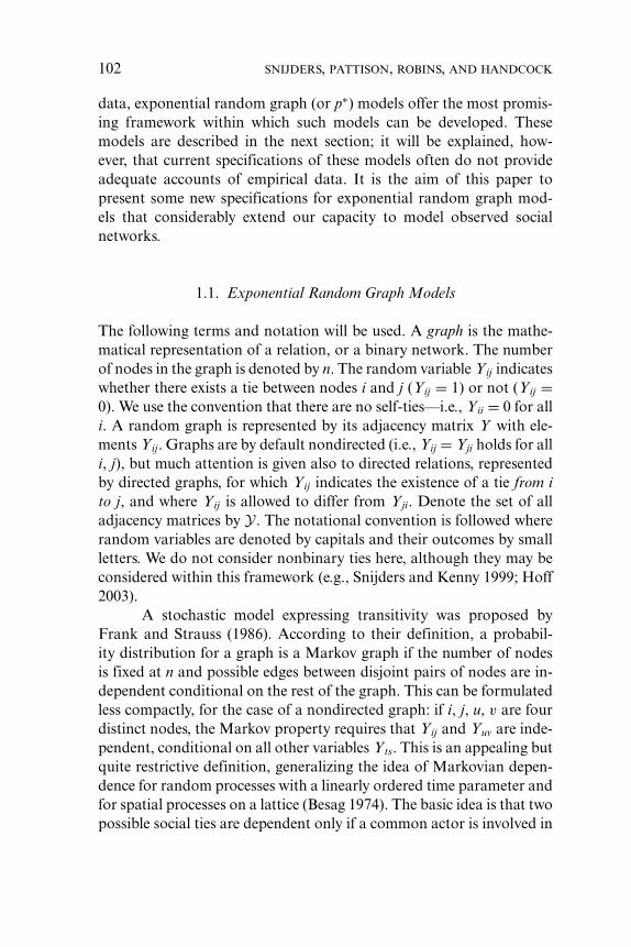
the Greek letters θ k and τ indicate parameters of the distribution, andψ(θ , τ ) is a normalizing constant ensuring that the probabilities sum to1. Replacing an index by the + sign denotes summation over the index,so yi+ is the degree of node i. A configuration (i , j 1, . . ., jk) is calleda k-star if i is tied to each of j 1, j 2, up to jk. For all k, the number ofk-stars in which node i is involved, is given by
(yi+k
). An edge is a one-
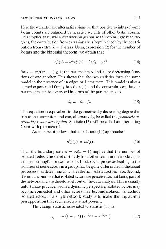
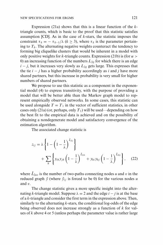
star, so S1(y) is also equal to the number of one-stars. Some of theseconfigurations are illustrated in Figure 1.
It may be noted that this family of distributions contains forθ 2 = . . . = θ n−1 = τ = 0 the trivial case of the Bernoulli graph—i.e., thepurely random graph in which all edges occur independently and havethe same probability eθ1/(1 + eθ1 ).
Frank and Strauss (1986) elaborated mainly the three-parametermodel where θ 3 = . . . = θ n−1 = 0, for which the probability distributiondepends on the number of edges, the number of two-stars, and the num-ber of transitive triads. They observed that parameter estimation forthis model is difficult, and they presented a simulation-based methodfor the maximum likelihood estimation of any one of the three parame-ters in this model, given that the other two are fixed at 0, which is only oftheoretical value. They also proposed the so-called pseudo-likelihood
104 SNIJDERS, PATTISON, ROBINS, AND HANDCOCK
FIGURE 1. Some configurations for nondirected graphs.
estimation method for estimating the complete vector of parameters.This is based on maximizing the pseudo-loglikelihood defined by
(θ ) =∑i< j
ln(
Pθ
{Yi j = yi j | Yuv = yuv for all u < v, (u, v) �= (i, j )
} ).
(3)
This method can be carried out relatively easily, as the algorithm isformally equivalent to a logistic regression. However, the properties ofpseudo-loglikelihood estimators have not been adequately establishedfor social networks. In analogous situations in spatial statistics, the maxi-mum pseudo-loglikelihood estimator has been observed to overestimatethe dependence in situations where the dependence is strong and to per-form adequately when the dependence is weak (Geyer and Thompson1992). For most social networks the dependence is strong and the max-imum pseudo-loglikelihood is suspect.
The paper by Frank and Strauss (1986) was seminal and led tomany papers published in the 1990s. In the first place, Frank (1991) andWasserman and Pattison (1996) proposed to use a model of this form,both for nondirected and for directed graphs, with arbitrary statisticsu(y) in the exponent. This yields the probability functions
Pθ {Y = y} = exp(θ ′u(y) − ψ(θ )
)y ∈ Y (4)
where y is the adjacency matrix of a graph or digraph and u(y) is anyvector of statistics of the graph. Wasserman and Pattison called thisfamily of distributions the p∗ model. As this is an example of what

NEW SPECIFICATIONS FOR ERGMS 105
statisticians call an exponential family of distributions (e.g., Lehmann1983) with u(Y ) as the sufficient statistic, the family also is called anexponential random graph model (ERGM).
Various extensions of this model to valued and multivariate re-lations were published (among others, Pattison and Wasserman 1999;Robins, Pattison, and Wasserman 1999), focusing mainly on subgraphcounts as the statistics included in u(y), motivated by the Hammersley-Clifford theorem (Besag 1974). To estimate the parameters, the pseudo-likelihood method continued to be used, although it was acknowledgedthat the usual chi-squared likelihood ratio tests were not warranted here,and there remained uncertainty about the qualities and meaning of thepseudo-likelihood estimator. The concept of Markovian dependenceas defined by Frank and Strauss was extended by Pattison and Robins(2002) to partial conditional independence, meaning that whether edgesYij and Yuv are independent conditionally on the rest of the graph de-pends not only on whether they share nodes but also on the pattern ofties in the rest of the graph. This concept will be used later in this paper.
Recent developments in general statistical theory suggestedMarkov chain Monte Carlo (MCMC) procedures both for obtainingsimulated draws from ERGMs, and for parameter estimation. MCMCalgorithms for maximum likelihood (ML) estimation of the parametersin ERGMs were proposed by Snijders (2002) and Handcock (2003).This method uses a general property of maximum likelihood estimatesin exponential families of distributions such as (4). That is to say, theML estimate is the value θ for which the expected value of the statisticsu(Y ) is precisely equal to the observed value u(y):
Eθu(Y) = u(y). (5)
In other words, the parameter estimates require the model to reproduceexactly the observed values of the sufficient statistics u(y).
The MCMC simulation procedure, however, brought to light se-rious problems in the definition of the model given by (1) and (2). Thesewere discussed by Snijders (2002), Handcock (2002a, 2002b, 2003), andRobins, Pattison, and Woolcock (2005), and they go back to a type ofmodel degeneracy discussed in a more general sense by Strauss (1986).A probability distribution can be termed degenerate if it is concentratedon a small subset of the sample space, and for exponential families thisterm is used more generally for distributions defined by parameters on

106 SNIJDERS, PATTISON, ROBINS, AND HANDCOCK
the boundary of the parameter space; near degeneracy here is definedby the distribution placing disproportionate probability on a small setof outcomes (Handcock 2003).
A simple instance of the basic problem with these models occursas follows. If model (1) is specified with only an edge parameter θ 1 anda transitivity parameter τ , while θ 1 has a moderate and τ a sufficientlypositive value, then the exponent in (1) is extremely large when y is thecomplete graph (where all edges are present—i.e., yij = 1 for all i, j)and much smaller for all other graphs that are not almost complete.This difference is so extreme that for positive values of τ—except forquite small positive values—and moderate values of θ 1, the probabilityis almost 1 that the density of the random graph Y is very close to 1. Onthe other hand, if τ is fixed at a positive value and the edge parameterθ 1 is decreased to a sufficient extent, a point will be reached where theprobability mass moves dramatically from nearly complete graphs topredominantly low density graphs. This model has been studied asymp-totically by Jonasson (1999) and Handcock (2002a). If τ is nonnega-tive, Jonasson shows that asymptotically the model produces only threetypes of distributions: (1) complete graphs, (2) Bernoulli graphs, and(3) mixture distributions with a probability p of complete graphs anda probability 1 − p of Bernoulli graphs. These distributions are notinteresting in terms of transitivity. This near-degeneracy is related tothe phase transitions known for the Ising and some other models (e.g.,Besag 1974; Newman and Barkema 1999). The phase transition wasstudied for the triangle model by Haggstrom and Jonasson (1999) andBurda, Jurkiewicz, and Krzywicki (2004), and for the two-star modelby Park and Newman (2004).
Some examples of more complex models are given in Sections 4and 5 below. The phase transition occurs in such models as a near dis-continuity of the expected value Eθu(Y ) as a function of θ—i.e., as theexistence of a value of θ where a plot of coordinates Eθuk(Y) graphedas a function of the coordinate θ k (or of other coordinates θ k′) showsa sudden and big increase, or jump (e.g., see, the Figure 16 a). Mathe-matically, the function still is continuous, but the derivative is extremelylarge. In many network data sets this increase of E θuk(Y) jumps rightover the observed value uk(y); and for the parameter value where thejump occurs—which has to be the parameter estimate satisfying the like-lihood equation (5)—the probability distribution of uk(y) has a bimodalshape, reflecting that here the random graph distribution is a mixture of
NEW SPECIFICATIONS FOR ERGMS 107
the low-density graphs produced to the left of the jump, and the almostcomplete graphs produced to its right. Hence, although the parame-ter estimate does reproduce the observation u(y) as the fitted expectedvalue, this expected value is far from the two modes of the fitted distri-bution. This fitted model does not give a satisfactory representation ofthe data. Illustrations are given in later sections.
One potential way out of these problems might be to conditionon the total number of ties—i.e., to consider only graphs having theobserved number of edges. However, Snijders (2002) showed that al-though conditioning on the total number of ties does sometimes lead toimproved parameter estimation, the mentioned problems still occur inmore subtle forms, and there still are many data sets for which satisfac-tory parameter estimates cannot be obtained.
A question, then, must be answered: To what extent does model(1) when applied to empirical data produce parameter estimates that arein, or too close to, the nearly degenerate area, resulting in the impossi-bility of obtaining satisfactory parameter estimates. A next question iswhether a model such as (1) will provide a good fit. Our overall experi-ence is that, although sometimes it is possible to attain parameter esti-mates that work well, even though they are close to the nearly degeneratearea, there are many empirically observed graphs having a moderate orlarge degree of transitivity and a low to moderate density, which cannotbe well represented by a model such as (1), either because no satisfac-tory parameter estimates can be obtained or because the fitted modeldoes not give a satisfactory representation of the observed network.This model offers little medium ground between a very slight tendencytoward transitivity and a distribution that is for all practical purposesconcentrated on the complete graph or on more complex “crystalline”structures as demonstrated in Robins, Pattison, and Woolcock (2005).
The present paper aims to extend the scope of modeling socialnetworks using ERGMs by representing transitivity not only by thenumber of transitive triads but in other ways that are in accordancewith the concept of partial conditional independence of Pattison andRobins (2002). We have couched this introduction in terms of the impor-tant issue of transitivity, but the modeling of transitivity also requiresattention to star parameters, or equivalently, aspects of the degree distri-bution. New representations for transitivity and the degree distributionin the case of nondirected graphs are presented in Section 3, preceded bya further explanation of simulation methods for the ERGM in Section 2.
108 SNIJDERS, PATTISON, ROBINS, AND HANDCOCK
After the technical details in Section 3, we present in Section 4 somenew modeling possibilities made possible by these specifications, basedon simulations, showing that these new specifications push back someof the problems of degeneracy discussed above. In Section 5 the newmodels are applied to data sets that hitherto have not been amenable toconvergent parameter estimation for the ERGM. A similar developmentfor directed relations is given in Section 6.
2. GIBBS SAMPLING AND CHANGE STATISTICS
Exponential random graph distributions can be simulated, and the pa-rameters can be estimated, by MCMC methods as discussed by Snijders(2002) and Handcock (2003). This is implemented in the computer pro-grams SIENA (Snijders et al. 2005) and statnet (Handcock et al. 2005).A straightforward way to generate random samples from such distri-butions is to use the Gibbs sampler (Geman and Geman 1983): cyclethrough the set of all random variables Yij (i �= j) and simulate each inturn according to the conditional distribution
Pθ {Yi j = yi j | Yuv = yuv for all (u, v) �= (i, j )}. (6)
Continuing this procedure a large number of times defines a Markovchain on the space of all adjacency matrices that converges to the desireddistribution. Instead of cycling systematically through all elements ofthe adjacency matrix, another possibility is to select one pair (i, j) ran-domly under the condition i �= j, and then generate a random value ofYij according to the conditional distribution (6); this procedure is calledmixing (Tierney 1994). Instead of Gibbs steps for stochastically up-dating the values Yij, another possibility is to use Metropolis-Hastingssteps. These and some other procedures are discussed in Snijders (2002).
For the exponential model (4), the conditional distributions (6)can be obtained as follows, as discussed by Frank (1991) and Wassermanand Pattison (1996). For a given adjacency matrix y, define by y(1)(i, j )and y(0)(i, j ), respectively, the adjacency matrices obtained by definingthe (i, j) element as y(1)
i j (i, j ) = 1 and y(0)i j (i, j ) = 0 and leaving all other
elements as they are in y, and define the change statistic with (i, j) elementby

NEW SPECIFICATIONS FOR ERGMS 109
zi j = u(y(1)(i, j )) − u(y(0)(i, j )). (7)
The conditional distribution (6) is formally given by the logistic regres-sion with the change statistics in the role of independent variables,
logit(Pθ
{Yi j = 1 | Yuv = yuv for all (u, v) �= (i, j )
} ) = θ ′zi j . (8)
This is also the form used in the pseudo-likelihood estimation procedure,shown in (3).
The change statistic for a particular parameter has an interpre-tation that is helpful in understanding the implications of the model.When multiplied by the parameter value, it represents the change inlog-odds for the presence of the tie due to the effect in question. For in-stance, in model (1), if an edge being present on (i, j) would thereby formthree new triangles, then according to the model the log-odds of that tiebeing observed would increase by 3τ due to the transitivity effect.
The problems with the exponential random graph distributiondiscussed in the preceding section reside in the fact that for specifica-tions of the statistic u(y) containing the number of k-stars for k ≥ 2or the number of transitive triads, if these statistics have positive pa-rameters, changing some value yij can lead to large increases in thechange statistic for other variables yuv. The change in yuv suggested bythese change statistics will even further increase values of other changestatistics, and so on, leading to an avalanche of changes which ulti-mately leads to a complete graph from which the probability of escape isnegligible—hence the near degeneracy. Note that this is not intrinsicallyan algorithmic issue—the algorithm merely reflects the full-conditionalprobability distributions of the model. The cause is that the underlyingmodel places significant mass on complete (or near complete) graphs.A theoretical analysis of these issues is given by Handcock (2003).
This can be illustrated more specifically by the special case of theMarkov model defined by (1) and (2) for nondirected graphs where onlyedge, two-star, and triangle parameters are present. The change statisticis
z1i j
z2i j
z3i j
=
1
y(0)i+(i, j ) + y(0)
j+(i, j )
L2i j
=
1
yi+ + yj+ − 2 yi j
L2i j
(9)

110 SNIJDERS, PATTISON, ROBINS, AND HANDCOCK
where y(0)(i, j ) denotes, as above, the adjacency matrix obtained from yby letting y(0)
i j (i, j ) = 0 and leaving all other yuv unaffected, and y(0)i+(i, j )
and y(0)j+(i, j ) are for this reduced graph the degrees of nodes i and j; while
L2ij is the number of two-paths connecting i and j,
L2i j =∑h �=i, j
yih yhj . (10)
The corresponding parameters are θ 1, θ 2, and τ . The avalanche effect,occurring for positive values of the two-star parameter θ 2 and the tran-sitivity parameter τ , can be understood as follows.
All the change statistics are elementwise nondecreasing functionsof the adjacency matrix y. Therefore, given that θ 2 and τ are positive,increasing some element yij from 0 to 1 will increase many of the changestatistics and thereby the logits (8). In successive simulation steps of theGibbs sampling algorithm, an accidental increase of one element yij willtherefore increase the odds that a next variable yuv will also obtain thevalue 1, which in the next simulation steps will further increase manyof the change statistics, etc., leading to the avalanche effect. Note thatthe maximum value of z2 is 2(n − 2) and the maximum of z3 is (n − 2),both of which increase indefinitely as the number of nodes of the graphincreases, and this large maximum value is one of the reasons for theproblematic behavior of this model. It may be tempting to reduce thiseffect by choosing the edge parameter θ 1 strongly negative. However,this forces the model toward the empty graph. If the two forces arebalanced, the combined effect is a mixture of (near) empty and (near)full graphs with a paucity of the intermediate graphs that are closerto realistic observations. If the Markov random graph model containsa balanced mixture of positive and negative star parameter values, thisavalanche effect can be smaller or even absent. This property is exploitedand elaborated in the following section.
3. PROPOSALS FOR NEW SPECIFICATIONS FOR STARAND TRANSITIVITY EFFECTS
We begin this section by considering proposals that will model all k-star parameters as a function of a single parameter. Since the number

NEW SPECIFICATIONS FOR ERGMS 111
of stars is a function of the degrees, this is equivalent to modeling thedegree distribution. Suitable functions will ensure that the avalancheeffect referred to in the previous section will not occur, or will at leastbe constrained. These steps can be taken within the framework of theMarkov dependence assumption.
We then turn to transitivity, which is more important from a the-oretical point of view but is treated after the models for k-stars andthe degree distribution because of the greater complexity of the graphstructures involved. The model for transitivity uses a new graph config-uration that we term a k-triangle. We model k-triangles in similar waysto the stars, in that all k-triangle parameters are modeled as a functionof a single parameter. But these new parameters are not encompassedby Markov dependence, and we need to relax the dependence assump-tion to partial conditional dependence. The discussion is principally fornondirected graphs; the case of directed graphs is presented more brieflyin a later section.
3.1. Geometrically Weighted Degrees and Related Functions
Expression (1)–(2) shows that the exponent of a Markov graph modelcan contain an arbitrary linear function of the k-star counts Sk, k =1, . . . , n − 1. These counts Sk are given by binomial coefficients, whichare independent polynomials of the node degrees yi+, Sk being a poly-nomial of degree k. But it is known that every function of the numbers 1through n − 1 can be expressed as a linear combination of polynomialsof degrees 1, . . . , n − 1. Therefore, any function of the degree distribu-tion (i.e., any function of the degrees that does not depend on the nodelabels) can be represented as a linear combination of the k-star countsS1, . . . , Sn−1. In other words, we have complete liberty to include anyfunction of the degree distribution in the exponent of (4) and still remainwithin the family of Markov graphs.
Saturated models for the degree sequence were discussed bySnijders (1991) and by Snijders and van Duijn (2002). These modelshave the virtue of giving a perfect fit to the degree distribution andcontrolling perfectly for the degrees when estimating and testing otherparameters, but at the expense of an exceedingly high number of pa-rameters and the impossibility to do more with the degree distributionthan describe it. Therefore we do not discuss these models here.

112 SNIJDERS, PATTISON, ROBINS, AND HANDCOCK
3.1.1. Geometrically Weighted Degree CountsA specification that has been traditional since the original paper byFrank and Strauss (1986) is to use the k-star counts themselves. Suchsubgraph counts, however, if they have positive weights θ k in the ex-ponent in (4), are precisely among the villains responsible for the de-generacy that has been plaguing ERGMs, as noted above. One primarydifficulty is that the model places high probability on graphs with largedegrees. A natural solution is to use a statistic that places decreasingweights on the higher degrees.
An elegant way is to use degree counts with geometrically de-creasing weights, as in the definition
u(d)α (y) =
n−1∑k=0
e−αkdk(y) =n∑
i=1
e−αyi+, (11)
where dk(y) is the number of nodes with degree k and α > 0 is a parametercontrolling the geometric rate of decrease in the weights. We refer to α asthe degree weighting parameter. For large values of α, the contributionof the higher degree nodes is greatly decreased. As α → 0 the statisticplaces increasing weight on the high degree graphs. This model is clearlya subclass of the model (4) where the vector of statistics is u(y) = d(y) ≡(d 0(y), . . . , d n−1(y)) but with a parametric constraint on the naturalparameters,
θk = e−αk k = 1, . . . , n − 1, (12)
which may be called the geometrically decreasing degree distributionassumption. This model is hence a curved exponential family (Efron1975). The statistic (11) will be called the geometrically weighted degreeswith parameter α.
As the degree distribution is a one-to-one function of the numberof k-stars, some additional insight can be gained by considering theequivalent model in terms of k-stars. Define
u(s)λ (y) = S2 − S3
λ+ S4
λ2− . . . + (−1)n−2 Sn−1
λn−3
=n−1∑k=2
(−1)k Sk
λk−2.
(13)
NEW SPECIFICATIONS FOR ERGMS 113
Here the weights have alternating signs, so that positive weights of somek-star counts are balanced by negative weights of other k-star counts.This implies that, when considering graphs with increasingly high de-grees, the contribution from extra k-stars is kept in check by the contri-bution from extra (k + 1)-stars. Using expression (2) for the number ofk-stars and the binomial theorem, we obtain that
u(s)λ (y) = λ2u(d)
α (y) + 2λS1 − nλ2 (14)
for λ = eα/(eα − 1) ≥ 1; the parameters α and λ are decreasing func-tions of one another. This shows that the two statistics form the samemodel in the presence of an edges or 1-star term. This model is also acurved exponential family based on (1), and the constraints on the starparameters can be expressed in terms of the parameter λ as
θk = −θk−1/λ. (15)
This equation is equivalent to the geometrically decreasing degree dis-tribution assumption and can, alternatively, be called the geometric al-ternating k-star assumption. Statistic (13) will be called an alternatingk-star with parameter λ.
As α → ∞, it follows that λ → 1, and (11) approaches
u(d)∞ (y) = d0(y). (16)
Thus the boundary case α = ∞(λ = 1) implies that the number ofisolated nodes is modeled distinctly from other terms in the model. Thiscan be meaningful for two reasons. First, social processes leading to theisolation of some actors in a group may be quite different from the socialprocesses that determine which ties the nonisolated actors have. Second,it is not uncommon that isolated actors are perceived as not being part ofthe network and are therefore left out of the data analysis. This is usuallyunfortunate practice. From a dynamic perspective, isolated actors maybecome connected and other actors may become isolated. To excludeisolated actors in a single network study is to make the implausiblepresupposition that such effects are not present.
The change statistic associated to statistic (11) is
zi j = − (1 − e−α
) (e−α yi+ + e−α y j+
)(17)
114 SNIJDERS, PATTISON, ROBINS, AND HANDCOCK
where y = y(0)(i, j ) is the reduced graph as defined above. This changestatistic is an elementwise nondecreasing function of the adjacency ma-trix, but the change becomes smaller as the degrees yi+ become larger,and for α > 0 the change statistic is negative and bounded below by2(e−α − 1). Thus, according to the criterion in Handcock (2003), a full-conditional MCMC for this model will mix close to uniformly. Thisshould help protect such models from the inferential degeneracy thathas hindered unconstrained models.
As discussed above, the change statistic aids interpretation. If theparameter value is positive, then we see that the conditional log-odds ofa tie on (i, j) is greater among high-degree actors. In a loose sense, this ex-presses a version of preferential attachment (Albert and Barabasi 2002)with ties from low degree to high degree actors being more probablethan ties among low degree actors. However, preference for high degreeactors is not linear in degree: the marginal gain in log-odds for connec-tions to increasingly higher degree partners is geometrically decreasingwith degree.
For instance, if α = ln(2) (i.e., λ = 2) in equation (17), for a fixeddegree of i, a connection to a partner j1 who has two other partners ismore probable than a connection to j2 with only one other partner, thedifference in the change statistics being 0.25. But if j1 and j2 have degrees5 and 6 respectively (from their ties to others than i), the difference in thechange statistics is less than 0.02. So, nodes with degree 5 and higher aretreated almost equivalently. Given these two effects – a preference forconnection to high degree nodes, and little differentiation among highdegree nodes beyond a certain point, we expect to see two differencesin outcomes from models with this specification compared to Bernoulligraphs with the same value for θ 1: a tendency for somewhat higherdegree nodes, and a tendency for a core-periphery structure.
3.1.2. Other Functions of DegreesOther functions of the node degrees could also be considered. It hasbeen argued recently (for an overview, see Albert and Barabasi 2002)that for many phenomena degree frequencies tend to 0 more slowly thanexponential functions—for example, as a negative power of the degrees.This suggests sums of reciprocals of degrees, or higher negative powersof degrees, instead of exponential functions such as (14). An alternativespecification of a slowly decreasing function that exploits the fact thatfactorials are recurrent in the combinatorial properties of graphs and

NEW SPECIFICATIONS FOR ERGMS 115
that is in line with recent applications of the Yule distribution to degreedistributions (see Handcock and Jones 2004), is a sum of ascendingfactorials of degrees,
u(y) =n∑
i=1
1(yi+ + c)r
(18)
where (d)r for integers d is Pochhammer’s symbol denoting the risingfactorial,
(d)r = d(d + 1) . . . (d + r − 1),
and the parameters c and r are natural numbers (1, 2, . . .). The associatedchange statistic is
zi j (y) = −r(yi+ + c)r+1
+ −r(y+ j + c)r+1
. (19)
The choice between this statistic and (13), and the choice of theparameters α or λ, c, and r, will depend on considerations of fit tothe observed network. Since these statistics are linearly independentfor different parameter values, several of them could in principle beincluded in the model simultaneously (although this will sometimeslead to collinearity-type problems and change the interpretation of theparameters).
3.2. Modeling Transitivity by Alternating k-Triangles
The issues of degeneracy discussed above suggest that in many empiricalcircumstances the Markov random graph model of Frank and Strauss(1986) is too restrictive. Our experience in fitting data suggests that prob-lems particularly occur with Markov models when the observed networkincludes not just triangles but larger “clique-like” structures that are notcomplete but do contain many triangles. Each of the three processesdiscussed in the introduction are likely to result in networks with suchdenser “clumps.” These are indeed the subject of much attention innetwork analysis (cohesive subset techniques), and the transitivity pa-rameter in Markov models (and perhaps the transitivity concept more

116 SNIJDERS, PATTISON, ROBINS, AND HANDCOCK
generally) can be regarded as the simplest way to examine such clique-like sections of the network because the triangle is the simplest cliquethat is not just a tie. But the linearity of the triangle count within theexponential is a source of the near-degeneracy problem in Markov mod-els, when observed incomplete cliques are somewhat large and hencecontain many triangles. What is needed to capture these “clique-ish”structures is a transitivity-like concept that expresses triangulation alsowithin subsets of nodes larger than three, and with a statistic that isnot linear in the triangle count but gives smaller probabilities to largecliquelike structures. Such a concept is proposed in this section.
From the problems associated with degeneracy, given the equiv-alence between the Markov conditional independence assumption andmodel (1), we draw two conclusions: (1) edges that do not share a tiemay still be conditionally dependent (i.e., the Markov dependence as-sumption may be too restrictive); (2) the representation of the socialphenomenon of transitivity by the total number of triangles is often toosimplistic, because the conditional log-odds of a tie between two socialactors often will not be simply a linear function of the total number oftransitive triangles to which this tie would contribute.
A more general type of dependence is the partial conditional in-dependence introduced by Pattison and Robins (2002), a definition thattakes into account not only which nodes are being potentially tied, butalso the other ties that exist in the graph—i.e., the dependence modelis realization-dependent. We propose a model that satisfies the moregeneral independence concept denoted here as [CD] for “ConditionalDependence.”
Assumption [CD]: Two edge indicators Yiv and Yuj are conditionallydependent, given the rest of the graph, only if one of the two followingconditions is satisfied:
1. They share a vertex—i.e., {i , v} ∩ {u, j} �= ∅ (the usual Markovcondition).
2. yiu = yvj = 1, i.e., if the edges existed they would be part of a four-cycle (see Figure 2).
This assumption can be phrased equivalently in terms of independence:If neither of the two conditions is satisfied, then Yiv and Yuj are condi-tionally independent, given the rest of the graph.

NEW SPECIFICATIONS FOR ERGMS 117
FIGURE 2. Partial conditional dependence when four-cycle is created.
One substantive interpretation of the partial conditional depen-dence assumption (2) is that the possibility of a four-cycle establishesthe structural basis for a “social setting” among four individuals (Patti-son and Robins 2002), and that the probability of a dyadic tie betweentwo nodes (here, i and v) is affected not just by the other ties of thesenodes but also by other ties within such a social setting, even if they donot directly involve i and v. A four-cycle assumption is a natural exten-sion of modeling based on triangles (three-cycles) and was first used byLazega and Pattison (1999) in an examination of whether such largercycles could be observed in an empirical setting to a greater extent thancould be accounted for by parameters for configurations involving atmost three nodes.
We now seek subgraph counts that can be included among thesufficient statistics u(y) in (4), expressing types of transitivity—thereforeincluding triangles—and leading to graph distributions conforming toassumption [CD]. Under the Markov assumption (1), Yiv is condition-ally dependent on each of Yiu, Yij, and Yjv, because these edge indica-tors share a node. If yiu = yjv = 1, the precondition in the four-cyclepartial conditional dependence (2), then Yiv is conditionally dependentalso on Yuj, and hence (cf. Pattison and Robins 2002) the Hammersley-Clifford theorem implies that the exponential model (4) could containthe statistic defined as the count of such configurations. We term thisconfiguration, given by
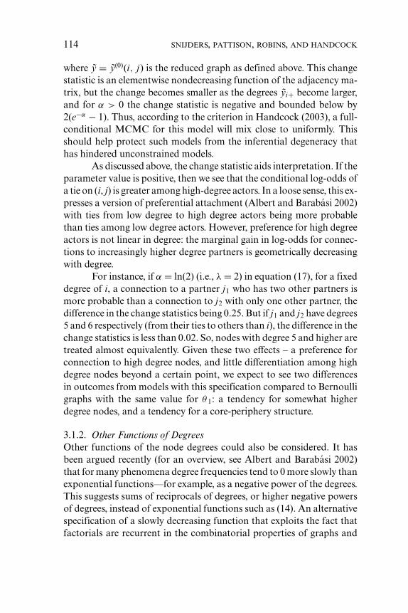
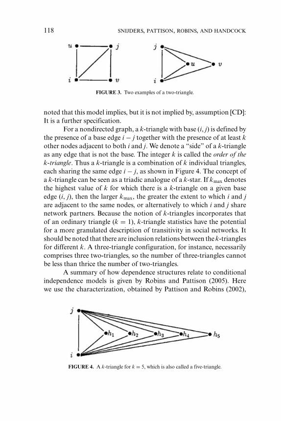
yiv = yiu = yi j = yu j = yjv = 1,
a two-triangle (see Figure 3). It represents the edge yij = 1 as part of thetriadic setting yij = yiv = yjv = 1 as well as the setting yij = yiu = yju = 1.
Elaborating this approach, we propose a model that satisfies as-sumption [CD] and is based on a generalization of triadic structures inthe form of graph configurations that we term k-triangles. It should be
118 SNIJDERS, PATTISON, ROBINS, AND HANDCOCK
FIGURE 3. Two examples of a two-triangle.
noted that this model implies, but it is not implied by, assumption [CD]:It is a further specification.
For a nondirected graph, a k-triangle with base (i, j) is defined bythe presence of a base edge i − j together with the presence of at least kother nodes adjacent to both i and j. We denote a “side” of a k-triangleas any edge that is not the base. The integer k is called the order of thek-triangle. Thus a k-triangle is a combination of k individual triangles,each sharing the same edge i − j, as shown in Figure 4. The concept ofa k-triangle can be seen as a triadic analogue of a k-star. If kmax denotesthe highest value of k for which there is a k-triangle on a given baseedge (i, j), then the larger kmax, the greater the extent to which i and jare adjacent to the same nodes, or alternatively to which i and j sharenetwork partners. Because the notion of k-triangles incorporates thatof an ordinary triangle (k = 1), k-triangle statistics have the potentialfor a more granulated description of transitivity in social networks. Itshould be noted that there are inclusion relations between the k-trianglesfor different k. A three-triangle configuration, for instance, necessarilycomprises three two-triangles, so the number of three-triangles cannotbe less than thrice the number of two-triangles.
A summary of how dependence structures relate to conditionalindependence models is given by Robins and Pattison (2005). Herewe use the characterization, obtained by Pattison and Robins (2002),
FIGURE 4. A k-triangle for k = 5, which is also called a five-triangle.

NEW SPECIFICATIONS FOR ERGMS 119
of the sufficient statistics u(y) in (4) of partial conditionally indepen-dent graph models. In the model proposed below, the statistics u(y)contain, in addition to those of the Markov model, parameters forall k-triangles. Such a model satisfies assumption [CD], which can beseen as follows. It was shown already above that this holds for two-triangles. Assuming appropriate graph realizations, [CD] implies thatevery possible edge in a three-triangle configuration can be condition-ally dependent on every other possible edge through one or the otherof the two-triangles, and hence as all possible edges are conditionallydependent, it follows from the characterization by Pattison and Robins(2002) that there is a parameter pertaining to the three-triangle in themodel. Induction on k shows that the Markovian conditional depen-dence (1) with the four-cycle partial conditional dependence (2) impliesthat there can be a parameter in the model for each possible k-triangleconfiguration.
Our proposed model contains the k-triangle counts, but includ-ing these all as separate statistics in the exponent of (4) would lead to alarge number of of statistical parameters. Therefore we propose a moreparsimonious model specifying relations between their coefficients inthis exponent, in much the same way as for alternating k-stars. Themodel expresses transitivity as the tendency toward a comparativelyhigh number of triangles, without too many high-order k-triangles be-cause this would lead to a (nearly) complete graph. Analogous to thealternating k-stars model, the k-triangle model described below impliesa possibly substantial increase in probability for an edge to appear inthe graph if it is involved in only one triangle, with further but smallerincreases in probability as the number of triangles that would be createdincreases (i.e., as the edge would form k-triangles of higher and higherorder). Thus, the increase in probability for creation of a k-triangle is adecreasing function of k. There is a substantively appealing interpreta-tion: If a social tie is not present despite many shared social partners,then there is likely to be a serious impediment to that tie being formed atall (e.g., impediments such as limitations to degrees and to the numberof nodes connected together in a very dense cluster, mutual antipathy, orgeographic distance, depending on the empirical context). In that case,the addition of even more shared partners is not likely to increase theprobability of the tie greatly.
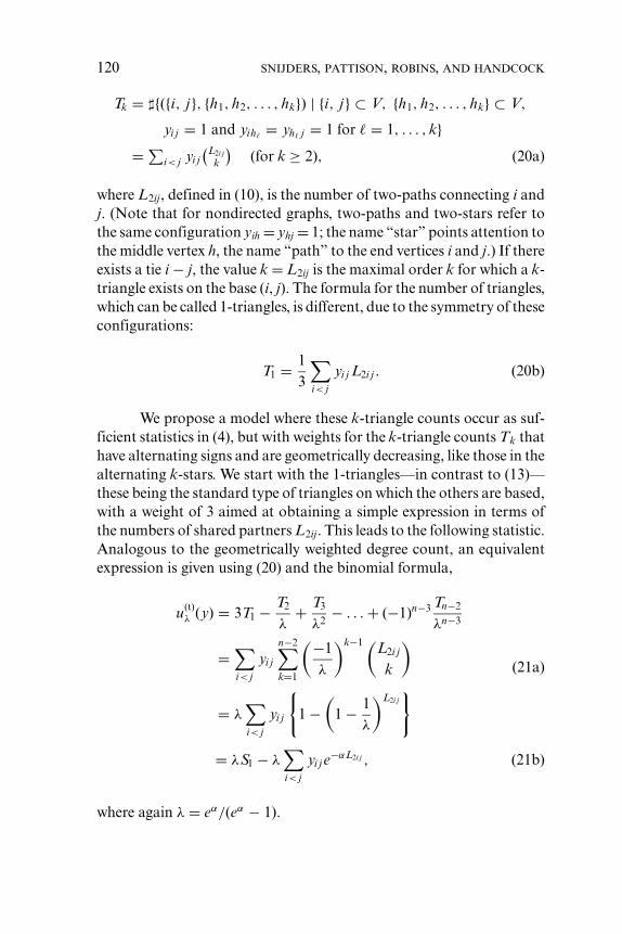
This is expressed mathematically as follows. The number of k-triangles is given by the formula
120 SNIJDERS, PATTISON, ROBINS, AND HANDCOCK
Tk = �{({i, j}, {h1, h2, . . . , hk}) | {i, j} ⊂ V, {h1, h2, . . . , hk} ⊂ V,
yi j = 1 and yih= yh j = 1 for = 1, . . . , k}
= ∑i< j yi j
(L2i jk
)(for k ≥ 2), (20a)
where L2ij, defined in (10), is the number of two-paths connecting i andj. (Note that for nondirected graphs, two-paths and two-stars refer tothe same configuration yih = yhj = 1; the name “star” points attention tothe middle vertex h, the name “path” to the end vertices i and j.) If thereexists a tie i − j, the value k = L2ij is the maximal order k for which a k-triangle exists on the base (i, j). The formula for the number of triangles,which can be called 1-triangles, is different, due to the symmetry of theseconfigurations:
T1 = 13
∑i< j
yi j L2i j . (20b)
We propose a model where these k-triangle counts occur as suf-ficient statistics in (4), but with weights for the k-triangle counts Tk thathave alternating signs and are geometrically decreasing, like those in thealternating k-stars. We start with the 1-triangles—in contrast to (13)—these being the standard type of triangles on which the others are based,with a weight of 3 aimed at obtaining a simple expression in terms ofthe numbers of shared partners L2ij. This leads to the following statistic.Analogous to the geometrically weighted degree count, an equivalentexpression is given using (20) and the binomial formula,
u(t)λ (y) = 3T1 − T2
λ+ T3
λ2− . . . + (−1)n−3 Tn−2
λn−3
=∑i< j
yi j
n−2∑k=1
(−1λ
)k−1 (L2i j
k
)
= λ∑i< j
yi j
{1 −
(1 − 1
λ
)L2i j} (21a)
= λS1 − λ∑i< j
yi j e−αL2i j , (21b)
where again λ = eα/(eα − 1).
NEW SPECIFICATIONS FOR ERGMS 121
Expression (21a) shows that this is a linear function of the k-triangle counts, which is basic to the proof that this statistic satisfiesassumption [CD]. As in the case of k-stars, the statistic imposes theconstraint τ k = − τ k−1/λ (k ≥ 3), where τ k is the parameter pertain-ing to Tk. The alternating negative weights counteract the tendency toforming big cliquelike clusters that would be inherent in a model withonly positive weights for k-triangle counts. Expression (21b) is (for α >
0) an increasing function of the numbers L2ij for which there is an edgei − j, but it increases very slowly as L2ij gets large. This expresses thatthe tie i − j has a higher probability accordingly as i and j have moreshared partners, but this increase in probability is very small for highernumbers of shared partners.
We propose to use this statistic as a component in the exponen-tial model (4) to express transitivity, with the purpose of providing amodel that will be better able than the Markov graph model to rep-resent empirically observed networks. In some cases, this statistic canbe used alongside T = T 1 in the vector of sufficient statistics, in othercases only (21a) (or, perhaps, only T 1) will be used—depending on howthe best fit to the empirical data is achieved and on the possibility ofobtaining a nondegenerate model and satisfactory convergence of theestimation algorithm.
The associated change statistic is
zi j = λ
{1 −
(1 − 1
λ
)L2i j}
+∑
h
{yih yjh
(1 − 1
λ
)L2ih
+ yhi yhj
(1 − 1
λ
)L2h j}
, (22)
where L2uv is the number of two-paths connecting nodes u and v in thereduced graph y (where yi j is forced to be 0) for the various nodes uand v.
The change statistic gives a more specific insight into the alter-nating k-triangle model. Suppose λ = 2 and the edge i − j is at the baseof a k-triangle and consider the first term in the expression above. Then,similarly to the alternating k-stars, the conditional log-odds of the edgebeing observed does not increase strongly as a function of k for val-ues of k above 4 or 5 (unless perhaps the parameter value is rather large
122 SNIJDERS, PATTISON, ROBINS, AND HANDCOCK
compared to other effects in the model). The model expresses the notionthat it is the first one to three shared partners that principally influencetransitive closure, with additional partners not substantially increasingthe chances of the tie being formed. The second and third terms of thechange statistic relate to situations where the tie completes a k-triangleas a side rather than as the base. For example, for the second term, theedge i − h is the base and h is a partner shared with j; the change statis-tic decreases as a function of the number of two-paths from i to h. Thismight be interpreted as actor i, already sharing many partners with h,feeling little impetus to establish a new shared partnership with j whois also a partner to h.
As was the case for the alternating k-stars, this statistic is con-sidered for λ ≥ 1, and the downweighting of higher-order k-triangles isgreater accordingly as λ is larger. Again, the boundary case λ = 1 has aspecial interpretation. For λ = 1 the statistic is equal to
u(t)1 (y) =
∑i< j
yi j I{L2i j ≥ 1}, (23)
the number of pairs (i, j) that are directly linked (yij = 1) but alsoindirectly linked (yih = yhj = 1 for at least one other node h). In this casethe change statistic is
zi j = I{L2i j ≥ 1} +∑
h
{yih yjh I{L2ih = 0} + yhi yhj I{L2h j = 0}}. (24)
3.3. Alternating Independent Two-Paths
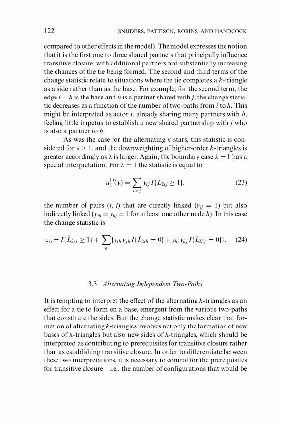
It is tempting to interpret the effect of the alternating k-triangles as aneffect for a tie to form on a base, emergent from the various two-pathsthat constitute the sides. But the change statistic makes clear that for-mation of alternating k-triangles involves not only the formation of newbases of k-triangles but also new sides of k-triangles, which should beinterpreted as contributing to prerequisites for transitive closure ratherthan as establishing transitive closure. In order to differentiate betweenthese two interpretations, it is necessary to control for the prerequisitesfor transitive closure—i.e., the number of configurations that would be
NEW SPECIFICATIONS FOR ERGMS 123
FIGURE 5. Two-independent two-paths (a) and five-independent two-paths (b).
the sides of k-triangles if there would exist a base edge. This means thatwe consider in addition the effect of connections by two-paths, irrespec-tive of whether the base is present or not. This is precisely analogousin a Markov model to considering both preconditions for triangles—i.e., two-stars or two-paths—and actual triangles. For Markov models,the presence of the two-path effect permits the triangle parameter tobe interpreted simply as transitivity rather than a combination of bothtransitivity and a chance agglomeration of many two-paths. Includingthe following configuration implies that the same interpretation is validin our new model.
We introduced k-triangles as an outcome of a four-cycle depen-dence structure. A four-cycle is a combination of two two-paths. Thesides of a k-triangle can be viewed as combinations of four-cycles. Moresimply, we construe them as independent (the graph-theoretical termfor nonintersecting) two-paths connecting two nodes.
Thus, we define k-independent two-paths, illustrated in Figure 5,as configurations (i , j , h1, . . ., hk) where all nodes h1 to hk are adjacentto both i and j, irrespective of whether i and j are tied. Their number isexpressed by the formula
Uk = �{({i, j}, {h1, h2, . . . , hk}) | {i, j} ⊂ V, {h1, h2, . . . , hk} ⊂ V,
i �= j, yih= yh j = 1 for = 1, . . . , k}
=∑i< j
(L2i j
k
)(for k �= 2) (25a)
U2 = 12
∑i< j
(L2i j
2
)(number of four-cycles); (25b)

124 SNIJDERS, PATTISON, ROBINS, AND HANDCOCK
the specific expression for k = 2 is required because of the symmetriesinvolved. The corresponding statistic, given as two equivalent expres-sions, of which the first one has alternating weights for the counts ofindependent two-paths while the second has geometrically decreasingweights for the counts of pairs with given numbers of shared partners,is
upλ(y) = U1 − 2
λU2 +
n−2∑k=3
(−1λ
)k−1
Uk
= λ∑i< j
{1 −
(1 − 1
λ
)L2i j}
,
(26a)
= λ(n
2
)−
∑i< j
e−αL2i j (26b)
where, in analogy to the statistic for the k-triangles, the extra factor 2is used for U 2 in (26a) in order for the binomial formula to yield theexpression (26b). As before, λ = eα/(eα − 1).
This is called the alternating independent two-paths statistic. Thechange statistic is
zi j =∑h �=i, j
{yjh
(1 − 1
λ
)L2ih
+ yhi
(1 − 1
λ
)L2h j}
. (27)
As for the alternating k-star and k-triangle statistics, the alternat-ing independent two-paths statistic can be generated by imposing theconstraint νk = − νk−1/λ, where νk is the parameter corresponding toUk.
For λ = 1 the statistic reduces to
up1(y) =
∑i< j
I{L2i j ≥ 1}, (28)
the number of pairs (i, j) that are indirectly connected by at least onetwo-path. This statistic is counterpart to statistic (23), the number ofpairs both directly and indirectly linked. Taken together they assess

NEW SPECIFICATIONS FOR ERGMS 125
effects for transitivity in precise analogy with triangles and two-starsfor Markov graphs. Since two nodes i and j are at a geodesic distance oftwo if they are indirectly but not directly linked, the number of nodes ata geodesic distance two is equal to (28) minus (23). The change statisticfor λ = 1 is
zi j =∑h �=i, j
{yjh I{L2ih = 0} + yhi I{L2h j = 0}}. (29)
3.4. Summarizing the Proposed Statistics
Summarizing the preceding discussion, we propose to model transitivityin networks by exponential random graph models that could contain inthe exponent u(y) the following statistics:
1. The total number of edges S1(y), to reflect the density of the graph;this is superfluous if the analysis is conditional on the total numberof edges—and this indeed is our advice.
2. The geometrically weighted degree distributions defined by (11), orequivalently the alternating k-stars (13), for a given suitable valueof α or λ, to reflect the distribution of the degrees.
3. Next to, or instead of the alternating k-stars: the number of two-starsS2(y) or sums of reciprocals or ascending factorials (18); the choicebetween these degree-dependent statistics will be determined by theresulting fit to the data and the possibility of obtaining satisfactoryparameter estimates.
4. The alternating k-triangles (21a) and the alternating independenttwo-paths (26a), again for a suitable value of λ (which should be thesame for the k-triangles and the alternating independent two-pathsbut may differ from the value used for the alternating k-stars), toreflect transitivity and the preconditions for transitivity.
5. Next to, or instead of, the alternating k-triangles: the triad countT(y) = T1(y), if a satisfactory estimate can be obtained for thecorresponding parameter, and if this yields a better fit as shownfrom the t-statistic for this parameter.
Of course, actor and dyadic covariate effects can also be added.The choice of suitable values of α and λ depends on the data set. Fitting

126 SNIJDERS, PATTISON, ROBINS, AND HANDCOCK
this model to a few data sets, we had good experience with λ = 2 or 3 andthe corresponding α = ln (2) or ln (1.5). In some cases it may be usefulto include the statistics for more than one value of λ—for example, λ =1 (with the specific interpretations as discussed above) together withλ = 3. Instead of being determined by trial and error, the parameters λ
(or α) can also be estimated from the data, as discussed in Hunter andHandcock (2005).
This specification of the ERGM satisfies the conditional depen-dence condition [CD]. This dependence extends the classical Markoviandependence in a meaningful way to a dependence within social settings.It should be noted, however, that this type of partial conditional de-pendence is satisfied by a much wider class of stochastic graph modelsthan the transitivity-based models proposed here. Parsimony of mod-eling leads to restricting attention primarily to the statistics proposedhere. Further modeling experience and theoretical elaboration will haveto show to what extent it is desirable to continue modeling by includingcounts of other higher-order subgraphs, representing more complicatedgroup structures.
4. NEW MODELING POSSIBILITIES WITH THESESPECIFICATIONS
In this section, we present some results from simulation studies of thesenew model specifications. This section is far from a complete explo-ration of the parameter space. It only provides examples of the types ofnetwork structures that may emerge from the new specifications. Moreparticularly, it illustrates how the new alternating k-triangle parameter-ization avoids certain problems with degeneracy that were noted abovein regard to Markov random graph models.
We present results for distributions of nondirected graphs of30 nodes. The simulation procedure is similar to that used in Robinset al. (2005). In summary, we simulate graph distributions using theMetropolis-Hastings algorithm from an arbitrary starting graph, choos-ing parameter values judiciously to illustrate certain points. Typically wehave simulation runs of 50,000, with a burn-in of 10,000, although whenMCMC diagnostics indicate that burn-in may not have been achievedwe carry out a longer run, sometimes up to half a million iterations.

NEW SPECIFICATIONS FOR ERGMS 127
FIGURE 6. A graph from an alternating k-star distribution.
We sample every 100th graph from the simulation, examining graphstatistics and geodesic and degree distributions.
4.1. Geometrically Weighted Degree Distribution
The graph in Figure 6 is from a distribution obtained by simulating withan edge parameter of −1.7 and a degree weighting parameter (for α =ln (2) = 0.693, corresponding to λ = 2) of 2.6. This is a low-densitygraph with 25 edges and a density of 0.06, and in terms of graph statis-tics is quite typical of graphs in the distribution. Even despite the lowdensity, the graph shows elements of a core-periphery structure, withsome relatively high degree nodes (one with degree 7), several isolatednodes, and some low degree nodes with connections into the higherdegree “core.” What particularly differentiates the graph from a com-parable Bernoulli graph distribution with a mean of 25 edges is thenumber of stars, especially higher order stars. For instance, the number
128 SNIJDERS, PATTISON, ROBINS, AND HANDCOCK
of four-stars in the graph is 3.5 standard deviations above that from theBernoulli distribution. This is the result of a longer tail on the degreedistribution, compensated by larger numbers of low degree nodes. (Forinstance, less than 2 percent of corresponding Bernoulli graphs have thecombination expressed in this graph of 18 or more nodes isolated or ofdegree 1, and of at least one node with degree 6 or above.) Because of thecore-periphery elements, the triangle count in the graph, albeit low, isstill 3.7 standard deviations above the mean from the Bernoulli distribu-tion. Monte Carlo maximum likelihood estimates using the procedureof Snijders (2002) as implemented in the SIENA program (Snijders et al.2005) reassuringly reproduced the original parameter values, with an es-timated edge parameter of –1.59 (standard error 0.35) and a significantestimated geometrically weighted degree parameter of 2.87 (S.E. 0.86).
It is useful to compare the geometrically weighted degree distri-bution, or alternatively alternating k-star graph distribution, of whichthe graph in Figure 6 is an example, against the Bernoulli distributionwith the same expected number of edges. Figure 7 is a scatterplot com-paring the number of edges against the alternating k-stars statistic forboth distributions. The figure demonstrates a small but discernible dif-ference between the two distributions in terms of the number of k-starsfor a given number of edges. There is also a tendency here for greaterdispersion of edges and alternating k-stars in the k-star distribution. Aswith our example graph, in the alternating k-star distributions there aremore graphs with high degree nodes, as well as graphs with more lowdegree nodes.
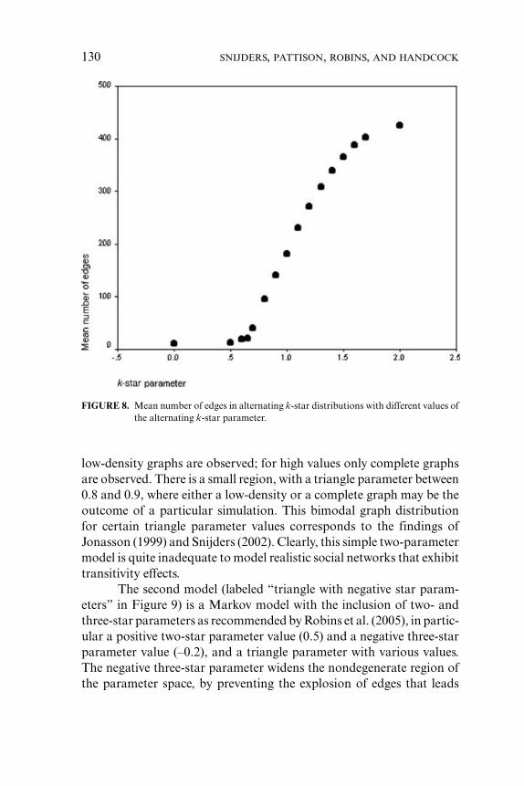
Finally, in Figure 8, we illustrate the behavior of the model asthe alternating k-star parameter increases. The figure plots the meannumber of edges for models with an edge parameter of –4.3 and varyingalternating k-star parameters, keeping λ = 2. Equation (13) implies that,as a graph becomes denser, the change statistic for alternating k-starsbecomes closer to its constant maximum, so that high-density distri-butions are very similar to Bernoulli graphs. For an alternating k-starparameter of 1.0 or above, the properties of individual graphs gener-ated within these distributions are difficult to differentiate from realiza-tions of Bernoulli graphs. Even so, the distributions themselves (exceptthose that are extremely dense) tend to exhibit much greater disper-sion in graph statistics, including in the number of edges. An importantpoint to note in Figure 8 is that there is a relatively smooth transitionfrom low-density to high-density graphs as the parameter increases,

NEW SPECIFICATIONS FOR ERGMS 129
FIGURE 7. Scatterplot of edges against alternating k-stars for Bernoulli and alternating k-star graph distributions.
without the almost discontinuous jumps that betoken degeneracy andare often exhibited in Markov random graph models with positive starparameters.
4.2. Alternating k-Triangles
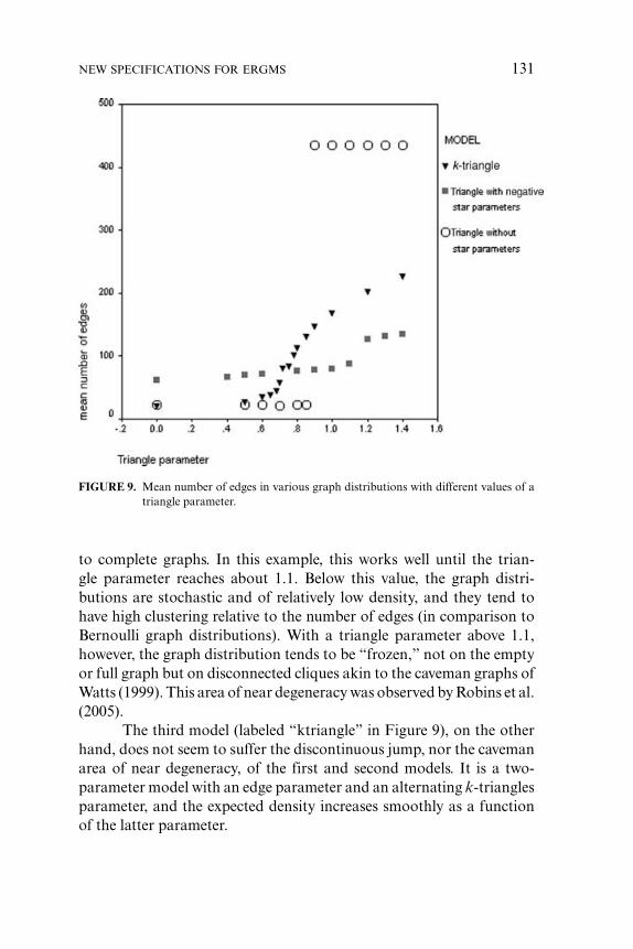
The degeneracy issue for transitivity models and the advance presentedby the alternating k-triangle specification are illustrated in Figure 9.This figure depicts the mean number of edges for three transitivity mod-els for various values of a transitivity-related parameter. Each of thesemodels contains a fixed edge parameter, set at –3.0, plus certain otherparameters.
The first model (labeled “triangle without star parameters” inthe figure) is a Markov model with simply the edge parameter and atriangle parameter. For low values of the triangle parameter, only very
130 SNIJDERS, PATTISON, ROBINS, AND HANDCOCK
FIGURE 8. Mean number of edges in alternating k-star distributions with different values ofthe alternating k-star parameter.
low-density graphs are observed; for high values only complete graphsare observed. There is a small region, with a triangle parameter between0.8 and 0.9, where either a low-density or a complete graph may be theoutcome of a particular simulation. This bimodal graph distributionfor certain triangle parameter values corresponds to the findings ofJonasson (1999) and Snijders (2002). Clearly, this simple two-parametermodel is quite inadequate to model realistic social networks that exhibittransitivity effects.
The second model (labeled “triangle with negative star param-eters” in Figure 9) is a Markov model with the inclusion of two- andthree-star parameters as recommended by Robins et al. (2005), in partic-ular a positive two-star parameter value (0.5) and a negative three-starparameter value (–0.2), and a triangle parameter with various values.The negative three-star parameter widens the nondegenerate region ofthe parameter space, by preventing the explosion of edges that leads
NEW SPECIFICATIONS FOR ERGMS 131
FIGURE 9. Mean number of edges in various graph distributions with different values of atriangle parameter.
to complete graphs. In this example, this works well until the trian-gle parameter reaches about 1.1. Below this value, the graph distri-butions are stochastic and of relatively low density, and they tend tohave high clustering relative to the number of edges (in comparison toBernoulli graph distributions). With a triangle parameter above 1.1,however, the graph distribution tends to be “frozen,” not on the emptyor full graph but on disconnected cliques akin to the caveman graphs ofWatts (1999). This area of near degeneracy was observed by Robins et al.(2005).
The third model (labeled “ktriangle” in Figure 9), on the otherhand, does not seem to suffer the discontinuous jump, nor the cavemanarea of near degeneracy, of the first and second models. It is a two-parameter model with an edge parameter and an alternating k-trianglesparameter, and the expected density increases smoothly as a functionof the latter parameter.
132 SNIJDERS, PATTISON, ROBINS, AND HANDCOCK
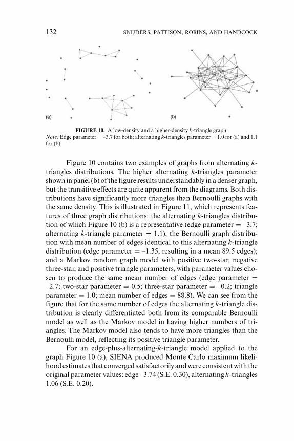
FIGURE 10. A low-density and a higher-density k-triangle graph.Note: Edge parameter = –3.7 for both; alternating k-triangles parameter = 1.0 for (a) and 1.1for (b).
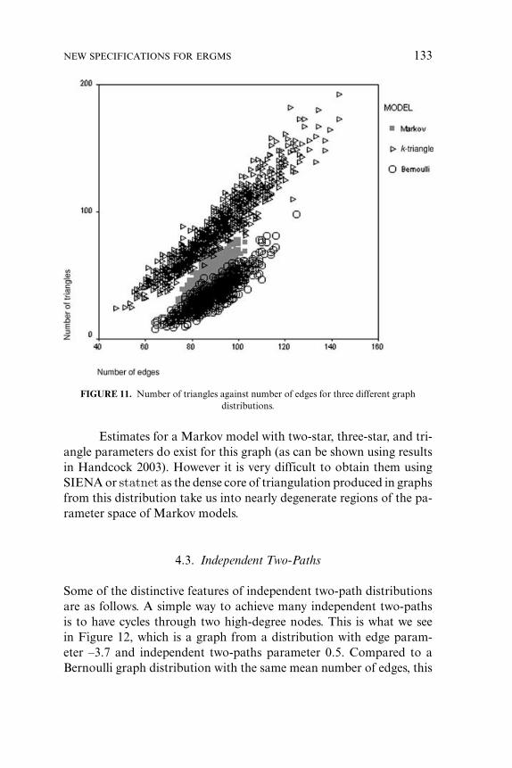
Figure 10 contains two examples of graphs from alternating k-triangles distributions. The higher alternating k-triangles parametershown in panel (b) of the figure results understandably in a denser graph,but the transitive effects are quite apparent from the diagrams. Both dis-tributions have significantly more triangles than Bernoulli graphs withthe same density. This is illustrated in Figure 11, which represents fea-tures of three graph distributions: the alternating k-triangles distribu-tion of which Figure 10 (b) is a representative (edge parameter = –3.7;alternating k-triangle parameter = 1.1); the Bernoulli graph distribu-tion with mean number of edges identical to this alternating k-triangledistribution (edge parameter = –1.35, resulting in a mean 89.5 edges);and a Markov random graph model with positive two-star, negativethree-star, and positive triangle parameters, with parameter values cho-sen to produce the same mean number of edges (edge parameter =–2.7; two-star parameter = 0.5; three-star parameter = –0.2; triangleparameter = 1.0; mean number of edges = 88.8). We can see from thefigure that for the same number of edges the alternating k-triangle dis-tribution is clearly differentiated both from its comparable Bernoullimodel as well as the Markov model in having higher numbers of tri-angles. The Markov model also tends to have more triangles than theBernoulli model, reflecting its positive triangle parameter.
For an edge-plus-alternating-k-triangle model applied to thegraph Figure 10 (a), SIENA produced Monte Carlo maximum likeli-hood estimates that converged satisfactorily and were consistent with theoriginal parameter values: edge –3.74 (S.E. 0.30), alternating k-triangles1.06 (S.E. 0.20).
NEW SPECIFICATIONS FOR ERGMS 133
FIGURE 11. Number of triangles against number of edges for three different graphdistributions.
Estimates for a Markov model with two-star, three-star, and tri-angle parameters do exist for this graph (as can be shown using resultsin Handcock 2003). However it is very difficult to obtain them usingSIENA or statnet as the dense core of triangulation produced in graphsfrom this distribution take us into nearly degenerate regions of the pa-rameter space of Markov models.
4.3. Independent Two-Paths
Some of the distinctive features of independent two-path distributionsare as follows. A simple way to achieve many independent two-pathsis to have cycles through two high-degree nodes. This is what we seein Figure 12, which is a graph from a distribution with edge param-eter –3.7 and independent two-paths parameter 0.5. Compared to aBernoulli graph distribution with the same mean number of edges, this

134 SNIJDERS, PATTISON, ROBINS, AND HANDCOCK
FIGURE 12. A graph from an independent two-path distribution.
graph distribution has substantially more stars, triangles, k-stars, k-triangles, and of course independent two-paths. The graph in Figure12 is dramatically different from graphs generated under a Bernoullidistribution.
With increasing independent two-paths parameters, the resultinggraphs tend to have two centralized nodes, but with more edges amongthe noncentral nodes. For lower (but positive) independent two-pathsparameters, however, only one centralized node appears, resulting ina single starlike structure, with several isolates. We know of no set ofMarkov graph parameters that can produce such large starlike struc-tures, without conditioning on degrees.
5. EXAMPLE: COLLABORATION BETWEENLAZEGA’S LAWYERS
Several examples will be presented based on a data collection by Lazega,described extensively in Lazega (2001), on relations between lawyers ina New England law firm (also see Lazega and Pattison 1999). As a

NEW SPECIFICATIONS FOR ERGMS 135
first example, the symmetrized collaboration relation was used betweenthe 36 partners in the firm, where a tie is defined to be present if bothpartners indicate that they collaborate with the other. The average degreeis 6.4, the density is 0.18, and degrees range from 0 to 13. Several actorcovariates were considered: seniority (rank number of entry in the firm),gender, office (there were three offices in different cities), years in thefirm, age, practice (litigation or corporate law), and law school attended(Yale, other Ivy League, or non–Ivy League).
The analysis was meant to determine how this collaboration re-lation could be explained on the basis of the three structural statisticsintroduced above (alternating combinations of two-stars, alternatingk-stars, and alternating independent two-paths), the more traditionalother structural statistics (counts of k-stars and triangles), and the co-variates. For the covariates X with values xi, two types of effect wereconsidered as components of the statistic u(y) in the exponent of theprobability function. The first is the main effect, represented by thestatistic
∑i
xi yi+.
A positive parameter for this model component indicates that actors ihigh on X have a higher tendency to make ties to others, which will con-tribute to a positive correlation between X and the degrees. This maineffect was considered for the numerical and dichotomous covariates.The second is the similarity effect. For numerical covariates such as ageand seniority, this was represented by the statistic
∑i, j
simi j yi j (30)
where the dyadic similarity variable simij is defined as
simi j = 1 − | xi − xj |dmax
x,
with dmaxx = max i,j |xi − xj | being the maximal difference on variable
X . The similarity effect for the categorical covariates, office and lawschool, was represented similarly using for sim ij the indicator functionI{xi = xj} defined as 1 if xi = xj and 0 otherwise. A positive parameter
136 SNIJDERS, PATTISON, ROBINS, AND HANDCOCK
for the similarity effect reflects that actors who are similar on X have ahigher tendency to be collaborating, which will contribute to a positivenetwork autocorrelation of X .
The estimations were carried out using the SIENA program(Snijders et al. 2005), version 2.1, implementing the Metropolis-Hastings algorithm for generating draws from the exponential ran-dom graph distribution, and the stochastic approximation algorithmdescribed in Snijders (2002). Since this is a stochastic algorithm, as isany MCMC algorithm, the results will be slightly different, dependingon the starting values of the estimates and the random number streamsof the algorithm. Checks were made for the stability of the algorithmby making independent restarts, and these yielded practically the sameoutcomes. The program contains a convergence check (indicated in theprogram as “Phase 3”): after the estimates have been obtained, a largenumber of Metropolis-Hastings steps is made with these parameter val-ues, and it is checked if the average of the statistics u(Y ) calculatedfor the generated graphs (with much thinning to obtain approximatelyindependent draws) is indeed very close to the observed values of thestatistics. Only results are reported for which this stochastic algorithmconverged well, as reflected by t-statistics less than 0.1 in absolute valuefor the deviations between all components of the observed u(y) andthe average of the simulations, which are the estimated expected valuesEθu(Y) (cf. (5) and also equation (34) in Snijders 2002).
The estimation kept the total number of ties fixed at the ob-served value, which implies that there is a not a separate parameterfor this statistic. This conditioning on the observed number of ties ishelpful for the convergence of the algorithm (for the example reportedhere, however, good convergence was obtained also without this con-ditioning). Effects were tested using the t-ratios defined as parameterestimate divided by standard error, and referring these to an approxi-mating standard normal distribution as the null distribution. The effectsare considered to be significant at approximately the level of α = 0.05when the absolute value of the t-ratio exceeds 2.
Some explorative model fits were carried out, and it turned outthat of the covariates, the important effects are the main effects of senior-ity and practice, and the similarity effects of gender, office, and practice.In Model 1 of Table 1, estimation results are presented for a model thatcontains the three structural effects: (1) geometrically weighted degreesfor α = ln(1.5) = 0.405 (corresponding to alternating combinations of
NEW SPECIFICATIONS FOR ERGMS 137
TABLE 1MCMC Parameter Estimates for the Symmetrized Collaboration Relation Among
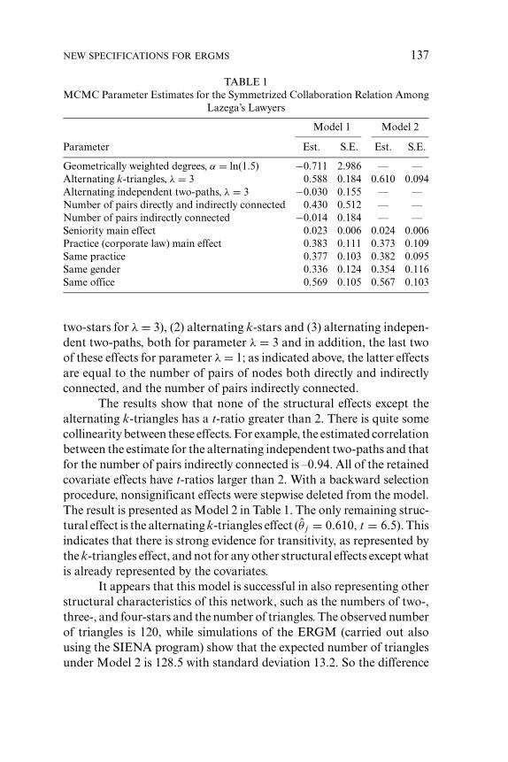
Lazega’s Lawyers
Model 1 Model 2
Parameter Est. S.E. Est. S.E.
Geometrically weighted degrees, α = ln(1.5) −0.711 2.986 — —Alternating k-triangles, λ = 3 0.588 0.184 0.610 0.094Alternating independent two-paths, λ = 3 −0.030 0.155 — —Number of pairs directly and indirectly connected 0.430 0.512 — —Number of pairs indirectly connected −0.014 0.184 — —Seniority main effect 0.023 0.006 0.024 0.006Practice (corporate law) main effect 0.383 0.111 0.373 0.109Same practice 0.377 0.103 0.382 0.095Same gender 0.336 0.124 0.354 0.116Same office 0.569 0.105 0.567 0.103
two-stars for λ = 3), (2) alternating k-stars and (3) alternating indepen-dent two-paths, both for parameter λ = 3 and in addition, the last twoof these effects for parameter λ = 1; as indicated above, the latter effectsare equal to the number of pairs of nodes both directly and indirectlyconnected, and the number of pairs indirectly connected.
The results show that none of the structural effects except thealternating k-triangles has a t-ratio greater than 2. There is quite somecollinearity between these effects. For example, the estimated correlationbetween the estimate for the alternating independent two-paths and thatfor the number of pairs indirectly connected is –0.94. All of the retainedcovariate effects have t-ratios larger than 2. With a backward selectionprocedure, nonsignificant effects were stepwise deleted from the model.The result is presented as Model 2 in Table 1. The only remaining struc-tural effect is the alternating k-triangles effect (θ j = 0.610, t = 6.5). Thisindicates that there is strong evidence for transitivity, as represented bythe k-triangles effect, and not for any other structural effects except whatis already represented by the covariates.
It appears that this model is successful in also representing otherstructural characteristics of this network, such as the numbers of two-,three-, and four-stars and the number of triangles. The observed numberof triangles is 120, while simulations of the ERGM (carried out alsousing the SIENA program) show that the expected number of trianglesunder Model 2 is 128.5 with standard deviation 13.2. So the difference

138 SNIJDERS, PATTISON, ROBINS, AND HANDCOCK
is less than 1 standard deviation. Fitting the model extended with thenumber of triangles did indeed lead to a nonsignificant effect for thenumber of triangles. The observed number of four-stars is 6091, andunder Model 2 the expected number of four-stars is equal to 6635 and thestandard deviation is 1042; so here also the difference between observedand expected value is less than 1 standard deviation. Thus, even thoughthese statistics are not directly fitted, the representation of the networkstructure by the alternating k-triangles together with the covariate effectsalso gives an adequate representation of these graph statistics.
The estimates for the covariates are hardly different from those inModel 1. Note that these can be interpreted as estimates of the covariateeffects on a log-odds scale, similar to effects in logistic regression models,except that they are controlled for the structural effects. This impliesthat exp (θ jd) is the multiplicative effect that a difference d on variablej has on the estimated odds of a tie. Seniority ranges from 1 to 36,so the more senior partners collaborate more with others, the oddsratio for the greatest difference of 35 being exp (0.024 × 35) = 2.32.Corporate lawyers have an odds of collaboration that is exp (0.373) =1.45 higher than those doing litigation, and having the same specialtymakes collaboration exp (0.382) = 1.47 more likely. The odds ratiorelated to having the same gender is exp (0.354) = 1.42, and that relatedto working in the same office is exp (0.567) = 1.76. All these odds ratiosare controlled for the structural transitivity effect. Summarizing, thereare especially large effects of seniority and of working in the same office,and slightly smaller but still large effects of doing corporate law, havingthe same specialty, and having the same gender; in addition, there is astrong transitivity effect.
The latter effect, represented by the alternating k-triangles, canbe interpreted as evidence that there are organizing principles in thisnetwork that go beyond homophilous selection in creating triangles.The nonsignificance of the weighted degrees effect suggests that thereare no other important effects distinguishing the partners in their levelof collaborative activity beside the effects of seniority and specialty; andthe significance of the k-triangle effect while controlling for the weighteddegrees effect indicates that the transitivity is not the result of popular-ity selection effects alone. In this law firm, it seems that collaborativestructures arise not just because of lawyers’ personal backgrounds; nordo they arise because of popular collaborators attracting less popularfollowers; rather, next to the covariate effects, there is a distinct balance

NEW SPECIFICATIONS FOR ERGMS 139
effect of self-organizing team formation, resulting in close-knit transi-tive structures. This conclusion is in line with the conclusions obtainedin earlier analyses of this data set (see Lazega 2001), but the results arenot directly comparable because analyses including effects of covariatesas well as structural transitivity effects were not published before.
The good fit in the sense of good reproduction of a variety ofother network statistics is not strongly dependent on the value of theparameter λ. Values λ = 2, 4, and 5 also yielded good results. The valuesλ = 1 and 6 were not satisfactory in this sense.
Model specifications containing the number of two-stars and oftransitive triangles also yielded convergence of the estimation algorithm,but it did not succeed well in reproducing the observed number of pairsof nodes tied directly and indirectly; this implies that the number ofpairs at a geodesic distance equal to two was not reproduced adequately.Thus, we can conclude that this example is a case where the traditionalMarkov random graph model for transitivity can be practically appliedbut that our new model specification yields a better fit to the data.
5.1. Parameter Sensitivity in Various Models
To illustrate the differences between the various model specificationsand the difficulties of some specifications, we present some simulationresults where a parameter is varied in fitted models. We contrast thespecification based on the number of triangles to the one using the al-ternating k-triangles. In addition, we compare models with and withoutconditioning on the total number of edges.
A model similar to Model 2 in Table 1 was fitted to this dataset, and then a long sequence of graphs was simulated by the MCMCprocedure, starting with the empty graph, where all parameters exceptone kept their fixed value, and one designated parameter slowly in-creased from a low to a high value, and then decreased again to the lowvalue, with 40,000 MCMC iteration steps for each value of this param-eter. The designated parameter was the one representing transitivity,being the number of triangles, or the alternating k-triangles. The figurespresent the generated values of the associated statistic after the 40,000iterations for each single parameter value.
Figure 13 gives the generated values for the model without con-ditioning on the number of edges (which for the number of triangles
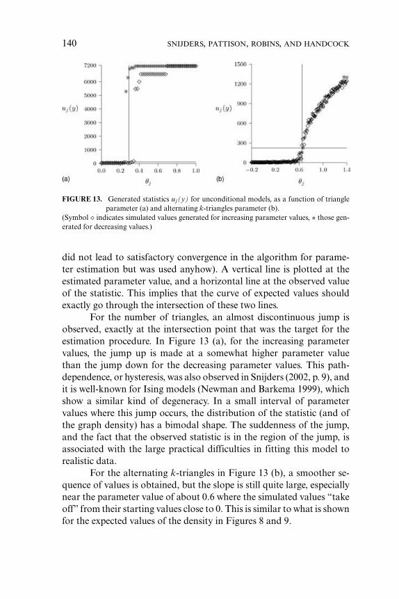
140 SNIJDERS, PATTISON, ROBINS, AND HANDCOCK
FIGURE 13. Generated statistics uj(y) for unconditional models, as a function of triangleparameter (a) and alternating k-triangles parameter (b).
(Symbol � indicates simulated values generated for increasing parameter values, ∗ those gen-erated for decreasing values.)
did not lead to satisfactory convergence in the algorithm for parame-ter estimation but was used anyhow). A vertical line is plotted at theestimated parameter value, and a horizontal line at the observed valueof the statistic. This implies that the curve of expected values shouldexactly go through the intersection of these two lines.
For the number of triangles, an almost discontinuous jump isobserved, exactly at the intersection point that was the target for theestimation procedure. In Figure 13 (a), for the increasing parametervalues, the jump up is made at a somewhat higher parameter valuethan the jump down for the decreasing parameter values. This path-dependence, or hysteresis, was also observed in Snijders (2002, p. 9), andit is well-known for Ising models (Newman and Barkema 1999), whichshow a similar kind of degeneracy. In a small interval of parametervalues where this jump occurs, the distribution of the statistic (and ofthe graph density) has a bimodal shape. The suddenness of the jump,and the fact that the observed statistic is in the region of the jump, isassociated with the large practical difficulties in fitting this model torealistic data.
For the alternating k-triangles in Figure 13 (b), a smoother se-quence of values is obtained, but the slope is still quite large, especiallynear the parameter value of about 0.6 where the simulated values “takeoff” from their starting values close to 0. This is similar to what is shownfor the expected values of the density in Figures 8 and 9.

NEW SPECIFICATIONS FOR ERGMS 141
FIGURE 14. Generated statistics uj(y) for conditional models, as a function of triangle pa-rameter (a) and alternating k-triangles parameter (b).
(Symbol � indicates values generated for increasing parameter values, ∗ those generated fordecreasing values.)
Analogous simulated values, but for models conditioning on theobserved number of edges, are given in Figure 14. Here we see in bothcases a much smoother process. The hysteresis effect for the numberof triangles is not observed any more, suggesting good mixing of theMCMC procedure, but this model still has quite a strong slope near theobserved value of the statistic. In Figure 14 (b), which combines condi-tional estimation with the alternating k-triangles statistic, the generatedvalues form a smooth pattern that confirms that estimation can proceedsmoothly for this model. The figures together illustrate that both work-ing with the newly proposed statistics rather than with the number oftriangles and conditioning on the number of edges contribute to betterpossibilities for parameter estimation. Combining both elements yieldsespecially good results.
6. DIRECTED RELATIONS
Directed relations are perhaps more frequent in social network researchthan nondirected relations. For directed relations, the requirement Yij =Yji for the adjacency matrix is dropped, and the oriented nature of tiesis reflected by using the term “arcs” rather than “edges.” Except for thenumber of ties, all statistics discussed above have multiple analogues forthe directed case, depending on the orientation of the ties. Rather than
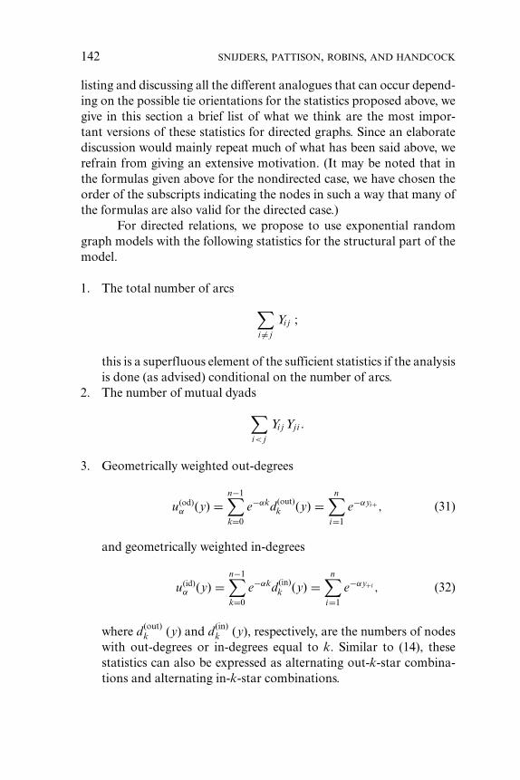
142 SNIJDERS, PATTISON, ROBINS, AND HANDCOCK
listing and discussing all the different analogues that can occur depend-ing on the possible tie orientations for the statistics proposed above, wegive in this section a brief list of what we think are the most impor-tant versions of these statistics for directed graphs. Since an elaboratediscussion would mainly repeat much of what has been said above, werefrain from giving an extensive motivation. (It may be noted that inthe formulas given above for the nondirected case, we have chosen theorder of the subscripts indicating the nodes in such a way that many ofthe formulas are also valid for the directed case.)
For directed relations, we propose to use exponential randomgraph models with the following statistics for the structural part of themodel.
1. The total number of arcs
∑i �= j
Yi j ;
this is a superfluous element of the sufficient statistics if the analysisis done (as advised) conditional on the number of arcs.
2. The number of mutual dyads
∑i< j
Yi j Yji .
3. Geometrically weighted out-degrees
u(od)α (y) =
n−1∑k=0
e−αkd (out)k (y) =
n∑i=1
e−αyi+, (31)
and geometrically weighted in-degrees
u(id)α (y) =
n−1∑k=0
e−αkd (in)k (y) =
n∑i=1
e−αy+i , (32)
where d (out)k (y) and d (in)
k (y), respectively, are the numbers of nodeswith out-degrees or in-degrees equal to k. Similar to (14), thesestatistics can also be expressed as alternating out-k-star combina-tions and alternating in-k-star combinations.

NEW SPECIFICATIONS FOR ERGMS 143
4. Next to, or instead of, the alternating k-star combinations: the num-ber of in-two-stars and the number of out-two-stars, reflecting thein-degree and out-degree variances.
5. The alternating transitive k-triangles defined by
λ∑i, j
yi j
{1 −
(1 − 1
λ
)L2i j}
(33)
and the alternating independent two-paths defined by
λ∑i, j
{1 −
(1 − 1
λ
)L2i j}
, (34)
where L2ij is still the number of two-paths defined by (10); the ori-entations implied by these formulas are illustrated in Figure 15.
6. Next to, or instead of the alternating transitive k-triangles: the countof transitive triads ∑
i, j,h
Yi j YjhYih
and the number of two-paths, the latter reflecting the covariancebetween in-degrees and out-degrees.
The change statistic for the geometrically weighted out-degreesis
zi j = − (1 − e−α
)e−α yi+ . (35)
The change statistic is still given for the alternating transitive k-trianglesby (22), and for the alternating independent two-paths by (27).
FIGURE 15. Transitive three-triangle (a) and three-independent two-paths (b).

144 SNIJDERS, PATTISON, ROBINS, AND HANDCOCK
6.1. Example: Friendship Between Lazega’s Lawyers
As an example of modeling a directed relation, we use the friendship re-lation between the 36 partners in the law firm studied by Lazega (2001).This is a network with density 0.21 and average degree 7.4. In-degreesvary from 2 to 16, out-degrees from 0 to 21. The larger variability ofthe degrees and skewness of the distribution of the out-degrees indicatesthat here it may be more difficult to obtain a well-fitting model than inthe preceding example. The same covariates are used as in the earlierexample. For effects of actor-level covariates X on directed relations,instead of the main effect we distinguish between (1) the activity effect,represented in u(y) by the statistic
∑i
xi yi+,
for which a positive parameter will tend to increase the correlation be-tween the covariate and the out-degrees; and (2) the popularity effect,represented by
∑i
xi y+i ,
which contributes to the correlation between the covariate and the in-degrees. The similarity effect connected to an actor-level covariate isdefined as for the undirected case.
Preliminary analyses showed that the most important effects ofcovariates are the similarity effect of working in the same office, andthe effects associated with seniority (rank number of entry in the firm)and practice (litigation versus corporate law). The same procedure forestimation was used as in the preceding example. A forward selectionprocedure using the effects listed above, with estimation conditional onthe total number of ties, led to the results presented in Table 2. Model 1contains, next to various covariate effects, the four structural effectsproposed above. This appeared not to give a good fit with respect to thenumber of out-k-stars for k = 2, 3, 4. Therefore the model was extendedwith the the numbers of in-two-stars, out-two-stars, and two-paths. Thismeans that the observed covariance matrix of the in- and out-degrees isfitted exactly. The results are presented in Table 2 as Model 2.
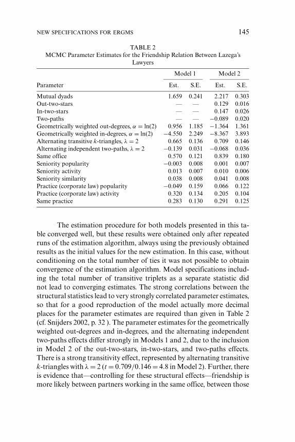
NEW SPECIFICATIONS FOR ERGMS 145
TABLE 2MCMC Parameter Estimates for the Friendship Relation Between Lazega’s
Lawyers
Model 1 Model 2
Parameter Est. S.E. Est. S.E.
Mutual dyads 1.659 0.241 2.217 0.303Out-two-stars — — 0.129 0.016In-two-stars — — 0.147 0.026Two-paths — — −0.089 0.020Geometrically weighted out-degrees, α = ln(2) 0.956 1.185 −1.364 1.361Geometrically weighted in-degrees, α = ln(2) −4.550 2.249 −8.367 3.893Alternating transitive k-triangles, λ = 2 0.665 0.136 0.709 0.146Alternating independent two-paths, λ = 2 −0.139 0.031 −0.068 0.036Same office 0.570 0.121 0.839 0.180Seniority popularity −0.003 0.008 0.001 0.007Seniority activity 0.013 0.007 0.010 0.006Seniority similarity 0.038 0.008 0.041 0.008Practice (corporate law) popularity −0.049 0.159 0.066 0.122Practice (corporate law) activity 0.320 0.134 0.205 0.104Same practice 0.283 0.130 0.291 0.125
The estimation procedure for both models presented in this ta-ble converged well, but these results were obtained only after repeatedruns of the estimation algorithm, always using the previously obtainedresults as the initial values for the new estimation. In this case, withoutconditioning on the total number of ties it was not possible to obtainconvergence of the estimation algorithm. Model specifications includ-ing the total number of transitive triplets as a separate statistic didnot lead to converging estimates. The strong correlations between thestructural statistics lead to very strongly correlated parameter estimates,so that for a good reproduction of the model actually more decimalplaces for the parameter estimates are required than given in Table 2(cf. Snijders 2002, p. 32 ). The parameter estimates for the geometricallyweighted out-degrees and in-degrees, and the alternating independenttwo-paths effects differ strongly in Models 1 and 2, due to the inclusionin Model 2 of the out-two-stars, in-two-stars, and two-paths effects.There is a strong transitivity effect, represented by alternating transitivek-triangles with λ = 2 (t = 0.709/0.146 = 4.8 in Model 2). Further, thereis evidence that—controlling for these structural effects—friendship ismore likely between partners working in the same office, between those
146 SNIJDERS, PATTISON, ROBINS, AND HANDCOCK
similar in seniority (this can be interpreted in part as a cohort effect),and those with the same practice. Those doing corporate law mentionmore friends than those doing litigation. The other covariate effects arenot significant. Other effects, such as the number of transitive tripletsand the numbers of three-stars and four-stars, also are represented ade-quately, each with a difference between observed and estimated expectedvalue of less than 1.5 standard deviation.
A positive effect of alternating k-triangles in the presence of anegative independent two-paths effect suggests that the friendship net-work tends to be cliquelike, with possibly several different denser clustersof friends. Because the geometrically weighted in-degree parameters arenegative, high in-degrees and high order in-stars are less likely in thisnetwork, unless of course they are implied by the transitive structureand therefore are involved in cliques of friends. So popular friends tendto be popular within clusters of dense friendships rather than betweenclusters.
Compared with the collaboration relation, modeling the friend-ship relation requires a much more complicated structural model. Thisnetwork is an example where modeling transitivity by the number oftransitive triplets by itself is not successful, whereas modeling transitiv-ity by the alternating transitive k-triangles is successful and also doesprovide a good fit for the number of transitive triplets.
6.2. Parameter Sensitivity in Two Models
For this model also, the sensitivity of generated statistics to the pa-rameter representing transitivity can yield insights in the possibility ofmodeling by using a particular model specification. Two models wereconsidered, both with conditioning on the observed number of ties: themodel in Table 2 and the corresponding model with the four new statis-tics replaced by the number of transitive triplets. For the latter model theparameter estimation did not converge satisfactorily, but the obtainedparameter values were used anyway. Figure 16 gives simulated statisticsfor a continuous MCMC chain of graphs, where all parameter valueswere fixed at these estimated values, except for the number of transitivetriplets (Figure 16 a) and the alternating k-triangles (Figure 16 b), whichstarted at a very low value, increased in little steps to a very high value,and then decreased again to the low value. Again, 40,000 iteration steps

NEW SPECIFICATIONS FOR ERGMS 147
FIGURE 16. Generated statistics uj(y) for two models, as a function of a transitive tripletsparameter (a) and an alternating k-triangles para-meter (b).
(Symbol � indicates values generated for increasing parameter values, ∗ those generated fordecreasing values.)
of the MCMC algorithm were made for each parameter value and theresulting value of the statistic corresponding to the changing parameteris represented in the figure.
For the transitive triplets model, there is a very strong jumpthat occurs right at the observed value of the statistic, indicating theimpossibility to adequately model this data set using this particularmodel—even when conditioning on the observed number of ties. A hys-teresis effect can again be discerned (for iteration runs of more than40,000, this would decrease and eventually disappear). For the alter-nating k-triangles model Figure 16 (b), there is a jump but it occursin a region representing antitransitivity (at a negative parameter valueof about –0.5), and does not invalidate the application of this modelfor this data set. The generated statistics for this model vary stochas-tically about a smooth function of this parameter in a wide regioncomprising the observed value of the statistic, which corresponds tothe possibility to indeed obtain adequate parameter estimates for thisspecification.
7. DISCUSSION
The methodology based on exponential random graph models, alsocalled p∗ models, of which the principles were introduced and elaborated

148 SNIJDERS, PATTISON, ROBINS, AND HANDCOCK
by (among others) Frank and Strauss (1986), Frank (1991), Wassermanand Pattison (1996), Pattison and Wasserman (1999), Robins, Pattison,and Wasserman (1999), Snijders (2002), and Handcock (2002b), andreviewed in Wasserman and Robins (2005), currently is the only sta-tistical methodology for representing transitivity and other structuralfeatures in nonlongitudinal network data. Its use has been hampered byproblems that now can be diagnosed—at least in part—as deficienciesin the specification of the sufficient statistics defining the exponentialmodel. The traditional specification, where transitivity is represented bythe number of transitive triangles or triplets as implied by the Markovassumption of Frank and Strauss (1986), does not allow a good repre-sentation of the quite strong but far from complete tendency to tran-sitivity that is commonly observed in social networks. A symptom ofthese problems is the difficulty to find maximum likelihood estimates,but the near degeneracy and poor fit of the implied model is the morefundamental issue.
In this paper we have proposed a new specification of networkstatistics defining the exponential random graph model. The new statis-tics are geometrically weighted degrees to represent degree hetero-geneity; alternating k-triangles to represent transitivity; and alternat-ing independent two-paths to represent the preconditions for transitiveconfigurations. Section 3.4 summarizes for nondirected graphs the re-sulting approach to model specification, and Section 6 gives the similarapproach for directed graphs. The new statistics are defined in such away that the model specification based on them does not imply, formoderately positive values of the parameter representing transitivity,the drive toward complete graphs that is inherent in the traditionalspecification. Therefore the new specification may be expected to avoidthe large degeneracy problems associated with the traditional specifi-cation. This is related to the fact that the new specification does notsatisfy the Markov conditional independence assumption of Frank andStrauss (1986), which often is too stringent. The new specification sat-isfies only a weaker type of partial conditional independence definedhere as assumption [CD], a specification of dependence concepts dis-cussed in Pattison and Robins (2002). However, the new statistics arenot a panacea: in the new models phase changes occur less often butthey are not completely excluded, as shown in the near discontinuity inFigure 16 (b). In this figure, however, the near discontinuity occurs at a

NEW SPECIFICATIONS FOR ERGMS 149
negative value of the transitivity parameter, which in sociological appli-cations is a relatively unimportant part of the parameter space. Our expe-rience up to now, illustrated by examples presented above, suggests thatthe models defined by these statistics can be used to give a good repre-sentation of the transitivity and degree heterogeneity in many observedsocial networks, also for data sets in which modeling on the basis of thetraditional specification, using only stars and the number of transitivetriplets or triangles, was not feasible. Further work is in progress thatconfirms the wider modeling possibilities opened up by the new spec-ifications. Obtaining maximum likelihood estimates under these spec-ifications by MCMC algorithms is relatively uncomplicated for manydata sets. The readily available computer programs SIENA (Snijderset al. 2005) and statnet (Handcock et al. 2005) can be used for thispurpose.
The statistics proposed here may look rather contrived at firstreading, but they are nevertheless a means to express that regions ofincomplete cliquelike structures will occur in social networks, but thatthese cannot be expressed merely by noting that the network containsmany triangles. The k-triangle parameters should therefore be inter-preted somewhat differently from the traditional transitivity parame-ters based on only the triangle count; in our first example we arguedthat the estimates give evidence for the emergence of close-knit transi-tive structures that might be interpretable as self-organizing team for-mation. Such a “higher order” interpretation is not really available inmodels containing only Markov transitivity based completely on theprevalence of single triangles in the network. The greater difficulty ininterpretation of the new statistics, as compared to the traditional spec-ification, seems unavoidable to us, given the complexity of empiricallyobserved social networks. Further experience with this model will beconducive to enhancing the interpretability of the parameters.
Other network statistics might also be possible to achieve thesemodeling possibilities. We do think that any statistics that achieve thiswill have some arbitrary elements, or seem contrived to some degree.This may have to do with the fact that network structure, as observed atone given moment, in most cases is the result of many different forcesand mechanisms that operated in a period—often of long duration—before the observation of the network, precluding a simple represen-tation of the dependencies within the network. One of the arguments

150 SNIJDERS, PATTISON, ROBINS, AND HANDCOCK
supporting the statistics proposed here is that they lead to a modelsatisfying the comparatively simple conditional dependence assumption[CD].
The statistics contain parameters (α or λ) that are supposed to befixed in the treatment given here, and they can be estimated in practice bytrying out some reasonable values. In the examples discussed earlier, thesensitivity of the conclusions for the precise value of this parameter wassmall. However, it is preferable to estimate this parameter statistically.The methods to do this are presented in Hunter and Handcock (2005).
Depending on the observed data set, it is still possible that degen-eracy problems occur even with these new specifications. More experi-ence with these models, and the further development of new models, isrequired before a satisfactory and well-balanced methodology for thestatistical modeling of networks will be attained. We think that the repre-sentation of social settings in particulars (Pattison and Robins 2002) willneed more attention and will be possible by incorporating extra modelelements. In some cases such extra model elements will be individualand dyadic covariates, or interactions of covariates with the structuresproposed above, which is easy to carry out as it remains within theframework of the exponential random graph model. In other cases themodel would have to be compounded with additional elements, such aslatent structure models like the Euclidean models of Hoff, Raftery, andHandcock (2002), the ultrametric models of Schweinberger and Snijders(2003), or the model-based clustering version of Tantrum, Handcock,and Raftery (2005); in still other cases, in the exponential model onecould include other complicated statistics in addition to those proposedhere, along the lines of Pattison and Robins (2002).
REFERENCES
Albert, Reka, and Albert-Laszlo Barabasi. 2002. “Statistical Mechanics of ComplexNetworks.” Review of Modern Physics 74:47–97.
Besag, Julian. 1974. “Spatial Interaction and the Statistical Analysis of LatticeSystems.” Journal of the Royal Statistical Society, Series B 36:192–225.
Boer, Peter, Mark Huisman, Tom A. B. Snijders, and Evelien P. H. Zeggelink. 2003.StOCNET: An Open Software System for the Advanced Statistical Analysis ofSocial Networks. Version 1.4. Groningen: ProGAMMA/ICS.
Burda, Zdzislaw, Jerzy Jurkiewicz, and Andre Krzywicki. 2004.“ Network Transi-tivity and Matrix Models.” Physical Review E69, 026106.

NEW SPECIFICATIONS FOR ERGMS 151
Davis, James A. 1970. “Clustering and Hierarchy in Interpersonal Relations: TestingTwo Theoretical Models on 742 Sociograms.” American Sociological Review35:843–52.
Davis, James A., and Samuel Leinhardt. 1972. “The Structure of Positive Inter-personal Relations in Small Groups.” Pp. 218–51 in Sociological Theories inProgress, vol. 2., edited by Joseph Berger. Boston: Houghton-Mifflin.
Efron, Bradley. 1975. “Defining the Curvature of a Statistical Problem (with Ap-plications to Second Order Efficiency),” Annals of Statistics 3:1189–242.
Frank, Ove. 1991. “Statistical Analysis of Change in Networks.” Statistica Neer-landica 45:283–93.
Frank, Ove, and David Strauss. 1986. “Markov Graphs.” Journal of the AmericanStatistical Association 81:832–42.
Geman, Stuart, and Donald Geman. 1983. “Stochastic Relaxation, gibbs Distribu-tions, and the Bayesian Restoration of Images.” IEEE Transaction on PatternAnalysis and Machine Intelligence 6:721–41.
Geyer, Charles J., and Elizabeth A. Thompson. 1992. “Constrained Monte Carlomaximum likehood calculations (with discussion).” Journal of the Royal Statis-tical Society, Series C, 54:657–99.
Haggstrom, Olle, and Johan Jonasson. 1999. “Phase Transition in the RandomTriangle Model.” Journal of Applied Probability 36:1101–15.
Handcock, Mark S. 2002a. “Specifying Models for Social Networks.” Presented atContact Networks and Transmission Dynamics of STDs, Centers for DiseaseControl and Prevention, National Center for HIV, STD, and TB PreventionMeeting, April 17–20, Washington, DC.
———. 2002b. “Statistical Models for Social Networks: Inference and Degener-acy.” Pp. 229–40 in Dynamic Social Network Modeling and Analysis: WorkshopSummary and Papers, edited by Ronald Breiger, Kathleen Carley, and PhilippaE. Pattison. Washington, DC: National Academies Press/National ResearchCouncil of the National Academies.
———. 2003. “Assessing Degeneracy in Statistical Models of Social Networks.”Working Paper No. 39, Center for Statistics and the Social Sciences, Universityof Washington, Seattle.
Handcock, Mark S., and James H. Jones. 2004. “Likelihood-Based Inference forStochastic Models of Sexual Network Formation.” Theoretical Population Biol-ogy 65:413–22.
Handcock, Mark S., David R. Hunter, Carter T. Butts, Steven M. Goodreau, andMartina Morris. 2005. statnet: An R package for the Statistical Analysis andSimulation of Social Networks. Manual, version 1.0. Center for Statistics and theSocial Sciences, University of Washington, Seattle.
Hoff, Peter D. 2003. “Bilinear Mixed Effects Models for Dyadic Data.” WorkingPaper No. 32, Center for Statistics and the Social Sciences, University of Wash-ington, Seattle.
Hoff, Peter D., Adrian E. Raftery, and Mark S. Handcock. 2002. “Latent SpaceApproaches to Social Network Analysis.” Journal of the American StatisticalAssociation 97:1090–98.

152 SNIJDERS, PATTISON, ROBINS, AND HANDCOCK
Holland, Paul W., and Samuel Leinhardt. 1975. “Local Structure in Social Net-works.” Pp. 1–45 in Sociololgical Methodology, vol. 6, edited by David R. Heise,Boston, MA: Blackwell Publishing.
Hunter, David R., and Mark S. Handcock. (Forthcoming). “Inference in CurvedExponential Family Models for Networks.” Journal of Graphical and Computa-tional Statistics.
Jonasson, Johan. 1999. “The Random Triangle Model.” Journal of Applied Proba-bility 36:852–67.
Lazega, Emmanuel. 2001. The Collegial Phenomenon: The Social Mechanisms ofCooperation Among Peers in a Corporate Law Partnership. Oxford, England:Oxford University Press.
Lazega, Emmanuel, and Philippa E. Pattison. 1999. “Multiplexity, GeneralizedExchange and Cooperation in Organizations: A Case Study.” Social Networks21:67–90.
Lehmann, Erich L. 1983. Theory of Point Estimation. New York: Wiley.McPherson, Miller, Lynn Smith-Lovin, and James M. Cook. 2001. “Birds of a
Feather: Homophily in Social Networks.” Annual Review of Sociology 27:415–44.
Newman, Mark E. J. 2003. “The Structure and Function of Complex Networks.”SIAM Review 45:167–256.
Newman, Mark E. J., and Gerard T. Barkema. 1999. Monte Carlo Methods inStatistical Physics. Oxford, England: Clarendon Press.
Park, Juyong, and Mark E. J. Newman. 2004. “Solution of the 2-star Model of aNetwork.” Condensed Matter Abstracts, cond-mat/0405457.
Pattison, Philippa E., and Garry L. Robins. 2002. “Neighbourhood Based Modelsfor Social Networks.” Pp. 301–37 in Sociological Methodology, vol. 22, editedby Ross M. Stolzenberg. Boston, MA: Blackwell Publishing.
Pattison, Philippa E., and Stanley Wasserman. 1999. “Logit Models and LogisticRegressions for Social Networks: II. Multivariate Relations.” British Journal ofMathematical and Statistical Psychology 52:169–93.
Robins, Garry L., Philippa E. Pattison, and Stanley Wasserman. 1999. “Logit Mod-els and Logistic Regressions for Social Networks: III. Valued Relations.” Psy-chometrika 64:371–94.
Robins, Garry L., and Philippa E. Pattison. 2005. “Interdependencies and So-cial Processes: Generalized Dependence Structures.” Pp. 192–214 in Modelsand Methods in Social Network Analysis, edited by Peter Carrington, JohnScott, and Stanley Wasserman. Cambridge, England: Cambridge UniversityPress.
Robins, Garry L., Philippa E. Pattison, and Jodie Woolcock. 2005. “Small and OtherWorlds: Global Network Structures from Local Processes.” American Journal ofSociology 110:894–936.
Schweinberger, Michael, and Tom A. B. Snijders. 2003. “Settings in Social Net-works: A Measurement Model.” Pp. 307–41 in Sociological Methodology, vol.23, edited by Ross M. Stolzenberg. Boston, MA: Blackwell Publishing.
Snijders, Tom A. B. 1991. “Enumeration and Simulation Methods for 0-1 Matriceswith Given Marginals.” Psychometrika 56:397–417.
NEW SPECIFICATIONS FOR ERGMS 153
———. 2002. “Markov Chain Monte Carlo Estimation of Exponential RandomGraph Models.” Journal of Social Structure, 3.2. Web journal available fromhttp://www2.heinz.cmu.edu/project/INSNA/joss/index1.html.
Snijders, Tom A. B., Christian E. G. Steglich, Michael Schweinberger, and MarkHuisman. 2005. Manual for SIENA version 2.1. Groningen, Netherlands: ICS.
Snijders, Tom A. B., and David A. Kenny. 1999. “The Social Relations Model forFamily Data: A Multilevel Approach.” Personal Relations 6:471–86.
Snijders, Tom A. B., and Marijtje A. J. van Duijn. 2002. “Conditional MaximumLikelihood Estimation under Various Specifications of Exponential RandomGraph Models.” Pp. 117–34 in Contributions to Social Network Analysis, In-formation Theory, and Other Topics in Statistics; A Festschrift in honour of OveFrank, edited by Jan Hagberg. Stockholm, Sweden: University of Stockholm,Department of Statistics.
Strauss, David. 1986. “On a General Class of Models for Interaction.” SIAM Review28:513–27.
Tantrum, Jeremy, Mark S. Handcock, and Adrian E. Raftery. 2005. “Model BasedClustering for Social Networks.” Working Paper No. 46, Center for Statisticsand the Social Sciences, University of Washington, Seattle.
Tierney, Luke. 1994. “Markov Chains for Exploring Posterior Distributions” (withdiscussion). Annals of Statistics 22:1701–62.
Wasserman, Stanley, and Philippa E. Pattison. 1996. “Logit Models and LogisticRegression for Social Networks: I. An Introduction to Markov Graphs and p
∗.”
Psychometrika 61:401–25.Wasserman, Stanley, and Garry L. Robins. 2005. “An Introduction to Random
Graphs, Dependence Graphs, and p∗.” Pp. 148–61 in Models and Methods in
Social Network Analysis, edited by Peter Carrington, John Scott, and StanleyWasserman. Cambridge, England: Cambridge University Press.
Watts, Duncan J. 1999. “Networks, Dynamics, and the Small-World Phenomenon.”American Journal of Sociology 105:493–527.