Matched drawability of graph pairs and of graph triples
24
Computational Geometry 43 (2010) 611–634 Contents lists available at ScienceDirect Computational Geometry: Theory and Applications www.elsevier.com/locate/comgeo Matched drawability of graph pairs and of graph triples ✩ Luca Grilli a,∗ , Seok-Hee Hong b , Giuseppe Liotta a , Henk Meijer c , Stephen K. Wismath d a Dipartimento di Ingegneria Elettronica e dell’Informazione, Università degli Studi di Perugia, Italy b School of Information Technologies, University of Sydney, Australia c Science Department, Roosevelt Academy, The Netherlands d Department of Mathematics & Computer Science, University of Lethbridge, Canada article info abstract Article history: Received 17 April 2009 Received in revised form 11 January 2010 Accepted 25 March 2010 Available online 31 March 2010 Communicated by D. Wagner Keywords: Graph drawing Matched drawings The contribution of this paper is twofold. It presents a new approach to the matched drawability problem of pairs of planar graphs and it provides four algorithms based on this approach for drawing the pairs outerplane, maximal outerpillar, outerplane, generalized outerpath, outerplane, wheel and wheel, wheel. Further, it initiates the study of the matched drawability of triples of planar graphs: it presents an algorithm to compute a matched drawing of a triple of cycles and an algorithm to compute a matched drawing of a caterpillar and two unlabeled level planar graphs. The results extend previous work on the subject and relate to existing literature about simultaneous embeddability and unlabeled level planarity. © 2010 Elsevier B.V. All rights reserved. 1. Introduction Let G 0 = ( V 0 , E 0 ) and G 1 = ( V 1 , E 1 ) be two planar graphs, each having n vertices such that there is a one-to-one mapping that matches each vertex of V 0 to a distinct vertex of V 1 . Graphs G 0 and G 1 are matched drawable with respect to the given one-to-one mapping if there exist two straight-line planar drawings Γ 0 and Γ 1 of G 0 and G 1 , respectively, such that every pair of matched vertices lies on one of n parallel lines and each line contains exactly two vertices. The pair Γ 0 , Γ 1 is a matched drawing of G 0 and G 1 with respect to the given one-to-one mapping. For example, consider the pair of graphs of Fig. 1(a), where the bold curves indicate the one-to-one mapping. Fig. 1(b) shows a matched drawing of G 0 and G 1 with respect to the given mapping; in the figure, the matched vertices lie on horizontal lines. A pair of planar graphs is matched drawable if it admits a matched drawing with respect to any given one-to-one mapping. The concept of matched drawability of a pair of planar graphs was first defined and studied in [9]. Matched drawings are a variant of simultaneous geometric embeddings first defined by Brass et al. in [2] and then studied in several papers, including [1,3,4,10,11,13,15,17]. A simultaneous geometric embedding of a pair G 0 , G 1 of planar graphs sharing their ver- tex set, consists of two straight-line planar drawings of the graphs such that every vertex has the same location in both drawings. If an edge is shared by the two graphs, then it is therefore represented by the same straight-line segment which makes it easy to visually discover common patterns in the drawings. However, the families of planar graphs that admit a simultaneous geometric embedding have been proven to be rather restricted (see, e.g., [2,10,18,19]). Requiring that the same ✩ An extended abstract of this paper appeared in the Proceedings of the 3rd International Workshop on Algorithms and Computation (WALCOM 2009) in Grilli et al. (2009) [20]. This research is partially supported by the MIUR Project “MAINSTREAM: Algorithms for Massive Information Structures and Data Streams” and by NSERC. * Corresponding author. E-mail addresses: [email protected] (L. Grilli), [email protected] (S.-H. Hong), [email protected] (G. Liotta), [email protected] (H. Meijer), [email protected] (S.K. Wismath). 0925-7721/$ – see front matter © 2010 Elsevier B.V. All rights reserved. doi:10.1016/j.comgeo.2010.03.005
Transcript of Matched drawability of graph pairs and of graph triples

Computational Geometry 43 (2010) 611–634
Contents lists available at ScienceDirect
Computational Geometry: Theory andApplications
www.elsevier.com/locate/comgeo
Matched drawability of graph pairs and of graph triples ✩
Luca Grilli a,∗, Seok-Hee Hong b, Giuseppe Liotta a, Henk Meijer c, Stephen K. Wismath d
a Dipartimento di Ingegneria Elettronica e dell’Informazione, Università degli Studi di Perugia, Italyb School of Information Technologies, University of Sydney, Australiac Science Department, Roosevelt Academy, The Netherlandsd Department of Mathematics & Computer Science, University of Lethbridge, Canada
a r t i c l e i n f o a b s t r a c t
Article history:Received 17 April 2009Received in revised form 11 January 2010Accepted 25 March 2010Available online 31 March 2010Communicated by D. Wagner
Keywords:Graph drawingMatched drawings
The contribution of this paper is twofold. It presents a new approach to the matcheddrawability problem of pairs of planar graphs and it provides four algorithms based on thisapproach for drawing the pairs 〈outerplane,maximal outerpillar〉, 〈outerplane,generalizedouterpath〉, 〈outerplane,wheel〉 and 〈wheel,wheel〉. Further, it initiates the study of thematched drawability of triples of planar graphs: it presents an algorithm to compute amatched drawing of a triple of cycles and an algorithm to compute a matched drawing of acaterpillar and two unlabeled level planar graphs. The results extend previous work on thesubject and relate to existing literature about simultaneous embeddability and unlabeledlevel planarity.
© 2010 Elsevier B.V. All rights reserved.
1. Introduction
Let G0 = (V 0, E0) and G1 = (V 1, E1) be two planar graphs, each having n vertices such that there is a one-to-onemapping that matches each vertex of V 0 to a distinct vertex of V 1. Graphs G0 and G1 are matched drawable with respect tothe given one-to-one mapping if there exist two straight-line planar drawings Γ0 and Γ1 of G0 and G1, respectively, such thatevery pair of matched vertices lies on one of n parallel lines and each line contains exactly two vertices. The pair Γ0, Γ1is a matched drawing of G0 and G1 with respect to the given one-to-one mapping. For example, consider the pair of graphs ofFig. 1(a), where the bold curves indicate the one-to-one mapping. Fig. 1(b) shows a matched drawing of G0 and G1 withrespect to the given mapping; in the figure, the matched vertices lie on horizontal lines. A pair of planar graphs is matcheddrawable if it admits a matched drawing with respect to any given one-to-one mapping.
The concept of matched drawability of a pair of planar graphs was first defined and studied in [9]. Matched drawingsare a variant of simultaneous geometric embeddings first defined by Brass et al. in [2] and then studied in several papers,including [1,3,4,10,11,13,15,17]. A simultaneous geometric embedding of a pair G0, G1 of planar graphs sharing their ver-tex set, consists of two straight-line planar drawings of the graphs such that every vertex has the same location in bothdrawings. If an edge is shared by the two graphs, then it is therefore represented by the same straight-line segment whichmakes it easy to visually discover common patterns in the drawings. However, the families of planar graphs that admit asimultaneous geometric embedding have been proven to be rather restricted (see, e.g., [2,10,18,19]). Requiring that the same
✩ An extended abstract of this paper appeared in the Proceedings of the 3rd International Workshop on Algorithms and Computation (WALCOM 2009)in Grilli et al. (2009) [20]. This research is partially supported by the MIUR Project “MAINSTREAM: Algorithms for Massive Information Structures and DataStreams” and by NSERC.
* Corresponding author.E-mail addresses: [email protected] (L. Grilli), [email protected] (S.-H. Hong), [email protected] (G. Liotta), [email protected] (H. Meijer),
[email protected] (S.K. Wismath).
0925-7721/$ – see front matter © 2010 Elsevier B.V. All rights reserved.doi:10.1016/j.comgeo.2010.03.005
612 L. Grilli et al. / Computational Geometry 43 (2010) 611–634
Fig. 1. (a) A pair of planar graphs G0 = (V 0, E0) and G1 = (V 1, E1) along with a one-to-one mapping between V 0 and V 1; the mapping is indicated bybold curves joining the pairs of matched vertices. (b) A matched drawing of G0 and G1 where matched vertices lie on horizontal lines.
vertices share only one of their coordinates, as is the case for matched drawings of pairs of graphs, is a natural relaxationto consider.
It is worth noting that matched drawability is also related to the well-known notion of level planarity (see, e.g., [7,21–23]). Namely, consider the 2n-vertex graph G consisting of the two disjoint n-vertex components G0 and G1. Consider allpossible one-to-one mappings between the vertices of G0 and G1. G0 and G1 are matched drawable if and only if for eachsuch mapping, G has a straight-line level planar drawing where every level contains exactly two matched vertices. As willbe shown in a subsequent section, matched drawability is also related to unlabeled level planar graphs, which have beenintroduced and studied in [12,14,16]. An unlabeled level planar graph G is a graph such that for any integer labeling ofits vertices there exists a straight-line planar drawing of G where the y-coordinate of each vertex matches its label. Thisimplies that an unlabeled level planar graph has a simultaneous geometric embedding with a path for any given one-to-onemapping between their vertex sets.
Finally, the study of matched drawings fits within the application framework recently described by Collins and Carpen-dale [5] who, motivated by exploring relationships between relational sets of data, present a system that matches vertices ofindependent drawings. Collins and Carpendale [5] compute the drawings independent of one another, which may give riseto many crossings among the edges that describe correspondences between vertices in different visualizations. By studyingmatched drawings we explore the possibility of visualizing pairs of graphs such that, if there is a bijection between theirvertices, then the bijection is emphasized by placing each pair of corresponding vertices along a distinct line of a set ofparallel lines. For a variant of matched drawings and a system that allows the visual correlation of two drawings of graphssee also [8].
The known results about matched drawability of graph pairs are described in [9]. The authors prove that not all planarpairs are matched drawable and also describe meaningful pairs of planar graphs that always admit a matched drawing.Among the different families of matched drawable graphs, they showed that every pair of trees with a bijection betweentheir vertices admits a matched drawing. Recall that not all tree pairs admit a simultaneous geometric embedding [19].
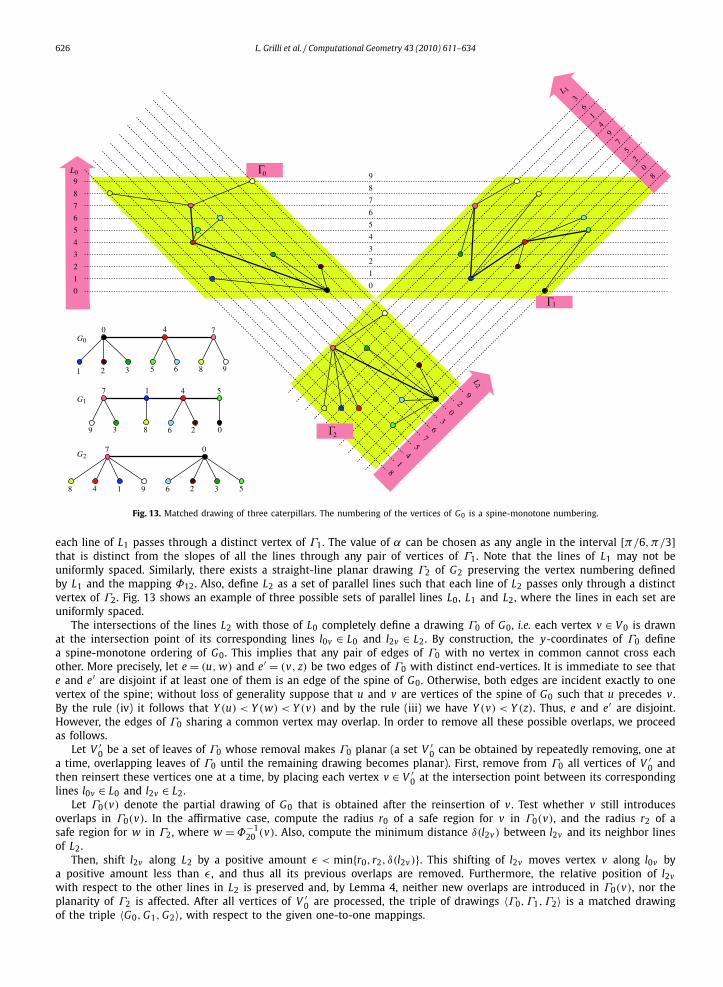
In this paper, we extend the results of [9] in different directions. Namely, we present both new pairs of matched drawableplanar graphs, and we initiate the study of matched drawings of triples of planar graphs. More precisely, let G0, G1, G2 be atriple of planar graphs that have the same number of vertices where there is a one-to-one mapping between the vertices ofany pair of graphs in the triple. Namely, two one-to-one mappings between the vertices of two pairs of graphs are specified,and by associativity the remaining one-to-one mapping is implicitly fixed. We say that the triple has a matched drawing withrespect to the given mappings if there are three straight-line planar drawings Γ0, Γ1, and Γ2, of G0, G1, and G2, respectively,such that: (i) each pair of drawings is a matched drawing of the corresponding pair of graphs with respect to the givenone-to-one mapping; and (ii) the parallel lines that describe a one-to-one mapping between two graphs do not intersectthe drawing of the remaining graph. We remark that without condition (ii) a matched drawing of a graph triple can beobtained by computing two matched drawings of two graph pairs, and by horizontally aligning the drawings of the graphs.However, in this way matched vertices of the leftmost and rightmost drawings lie on a set of parallel lines that overlap thein-between drawing. Therefore, this second requirement makes easier the visual correlation of graph pairs in the drawingand resembles the classical edge-region crossing-free constraint for cluster planarity [24]. Fig. 13 shows an example of amatched drawing of three graphs each having ten vertices; the three one-to-one mappings are represented by numberingthe vertices of the three graphs with integers from 0 to 9. A triple of planar graphs is matched drawable if it has a matcheddrawing for any given one-to-one mapping between the vertices of any pair of graphs in the triple. Our main results can beoutlined as follows.
1. We present a novel approach for computing matched drawings of pairs of planar graphs. This technique is based ona suitable labeling of the vertices of the graphs and on characterizing vertex levelings of graphs that always admita level planar realization. In this respect, our results can be related to the well-known research regarding level pla-narity and unlabeled level planarity (see [12,16]). As application examples of the proposed technique, we prove that

L. Grilli et al. / Computational Geometry 43 (2010) 611–634 613
the following pairs admit a matched drawing: 〈outerplane,maximal outerpillar〉, 〈outerplane,generalized outerpath〉,〈outerplane,wheel〉 and 〈wheel,wheel〉.
2. We introduce and study the notion of matched drawing for a triple of planar graphs. Using this concept we discovernew differences between matched drawability and simultaneous drawability. Namely, while it is known that triples ofgraphs with the same vertex set may not have a simultaneous geometric embedding even in the case that they aresimple paths [2], it turns out that a triple consisting of a caterpillar and two unlabeled level planar graphs [16] isalways matched drawable.
3. We exploit the drawing technique of the item above, combined with a suitable sequence of geometric translations, toshow that every triple of cycles admits a matched drawing.
The focus of the present paper is on proving the existence of matched drawings of graph pairs and of graph triples. Ourproofs are constructive, but some of our constructions can lead to drawings of exponential area. Assuming the real RAMmodel of computation, all the described algorithms run in polynomial time and most of them run in linear time.
The remainder of the paper is organized as follows. Preliminaries can be found in Section 2. Our approach for computingmatched drawings of graph pairs is described in Section 3. Matched drawings of graph triples are discussed in Section 4.Finally, Section 5 lists some open problems.
2. Preliminaries
We assume that the reader is familiar with standard notions of graph drawing [6,24–26]. Let G be a simple planar graph.A drawing Γ of G maps each vertex of G to a distinct point in the plane and each edge to a simple Jordan curve connectingthe points that represent its end-vertices. Drawing Γ is planar if no two distinct edges intersect except at common end-vertices. Drawing Γ is a straight-line planar drawing if it is planar and all its edges are represented by straight-line segments.G is planar if it admits a planar drawing.
A planar drawing Γ of G partitions the plane into topologically connected regions called the faces defined by Γ . Theunbounded face is called the external face; the other faces are the internal faces. A face f is represented by the circularordering of vertices and edges that are encountered when walking on its boundary in the clockwise direction if f is internal,and in the counterclockwise direction if f is external. A planar embedding of a planar graph G is an equivalence class ofplanar drawings that define the same set of faces for G . A planar graph G together with the description of a set of faces iscalled an embedded planar graph.
Let G be an embedded planar graph. A drawing of G is embedding preserving if it maintains the given planar embedding;otherwise, the drawing of G is not-embedding preserving. In this paper, we shall sometimes assume as input a graph Gwith a given planar embedding and compute planar drawings that do not preserve the given planar embedding.
The weak dual G∗ of G is a graph whose vertices correspond to the internal faces of G with an edge between two verticesif the corresponding internal faces in G share one or more edges.
A wheel is a graph consisting of a cycle plus a vertex, called the center of the wheel, that is connected to all the verticesof the cycle. A fan is a graph formed by a path plus a vertex, called the apex, that is connected to all the vertices of thepath; a fan can be obtained from a wheel by removing an edge that is not incident to its center.
An outerplanar graph is a graph that admits a planar embedding such that all vertices are on the same face. Suchan embedding is called an outerplanar embedding and the face containing all the vertices is referred to as the unboundedor the external face. An outerplanar graph is a maximal outerplanar graph if the addition of any new edge would destroyits outerplanarity; or equivalently, a biconnected outerplanar graph in which every internal face is defined by a three-cycle.Note that a biconnected outerplanar graph has a unique external face, which is defined by a Hamiltonian cycle. An outerplanegraph is an outerplanar graph with a given outerplanar embedding.
Let G be a maximal outerplane graph. If G has at least three vertices, then its internal faces are triangular and G∗ isa tree whose nodes have degree at most three. Note that G always contains at least two vertices of degree two. (This isimmediate when G has exactly three vertices. When G has more than three vertices, it is implied by the observation thatevery vertex v of G of degree two belongs to a face that is a leaf of G∗ and every leaf of G∗ corresponds to a face of G thatcontains exactly one vertex of degree two.)
An unlabeled level planar graph G (also known as an ULP graph [12,16]) is a graph such that for any integer labeling ofits vertices there exists a straight-line planar drawing of G where the y-coordinate of each vertex matches its labels. ULPgraphs can be distinguished into ULP graphs with duplicate labels and ULP graphs with distinct labels based on whether multiplevertices per level are allowed. Note that the set of ULP graphs with duplicate labels is strictly contained in the set of ULPgraphs with distinct labels. In the present paper, we consider only ULP graphs with distinct labels, which will be referredto as simply ULP graphs.
3. Matched drawings of graph pairs
Let G0 = (V 0, E0) and G1 = (V 1, E1) be two planar graphs such that |V 0| = |V 1| = n. Let Φ : V 0 → V 1 be a one-to-onemapping that matches every vertex v ∈ V 0 to a distinct vertex w ∈ V 1, i.e. w = Φ(v) and v = Φ−1(w). Let Γ0 and Γ1 betwo straight-line planar drawings of G0 and G1, respectively. The pair of drawings 〈Γ0,Γ1〉 is a matched drawing of G0 and

614 L. Grilli et al. / Computational Geometry 43 (2010) 611–634
G1, with respect to the one-to-one mapping Φ , if there exist n parallel lines such that each line contains exactly two matchedvertices. A pair of planar graphs 〈G0, G1〉 is matched drawable if it admits a matched drawing for any possible one-to-onemapping Φ between their vertices. In this section, we describe pairs 〈G0, G1〉 of planar graphs that are matched drawable.Without loss of generality, we shall assume in the following that any two matched vertices have the same y-coordinate inthe computed drawings.
In [9], it has been proven that every pair 〈T0, T1〉 where both T0 and T1 are trees is matched drawable. A matcheddrawing of two trees is constructed by a vertex addition strategy that alternately chooses the next vertex to be drawn fromT0 and from T1: T0 determines which vertex is placed in odd steps at y-coordinates n − 1,n − 2, . . . , �n/2� + 1 while T1determines which vertex is placed in even steps at y-coordinates 0,1, . . . , �n/2�. We extend this result by presenting newpairs of matched drawable graphs. This is done by using a drawing approach that looks similar but is also quite differentfrom the one of [9].
The main idea behind our new approach is to separate the role that the two graphs have in the computation. Based onthe topology of one of the two graphs, the vertices are given one of two labels. Based on the topology of the other graph,the y-coordinates are defined. Finally, the matched drawing is computed. More precisely, our approach can be described asconsisting of the following three main phases.
1. Labeling phase. Vertices of V 0 and of V 1 are associated with labels in the set {B, T } such that matched vertices have thesame label. Such a labeling, called a BT-labeling, specifies that vertices labeled as B (“Bottom”) will be drawn “below”those labeled as T (“Top”). The BT-labeling exclusively depends on the topology of G1. Namely, based on the topologyof G1 a BT-labeling of the vertices of V 1 is initially computed and then each vertex of G0 is given the label of thecorresponding vertex of G1.
2. Leveling phase. Let Y = {y0, y1, . . . , yn−1} be a set of n distinct non-negative integers. In this phase, matched vertices areassociated with numbers in set Y such that every vertex labeled B is given a number smaller than any vertex labeled T .Such an assignment of numbers in set Y to the vertices is called a label-preserving level assignment and it is computedby considering only the topology of G0.In particular, this phase is accomplished by constructing a straight-line planar drawing of G0 such that: (i) the verticeshave distinct non-negative integer y-coordinates; (ii) every vertex labeled B is given an y-coordinate strictly smallerthan any vertex labeled T .
3. Matching phase. A matched drawing 〈Γ0,Γ1〉 is obtained by computing a straight-line planar drawing of G1, such thatthe y-coordinates of the vertices are those defined by the label-preserving level assignment.
The matching phase relies on proving the following property: for any label-preserving level assignment of the verticesof G1, there always exists a straight-line planar drawing of G1 in which every vertex is given an y-coordinate equal to itslevel number. This will be clarified in the following subsections. It is worth noting that the graphs of the pairs that we studyin the next sections may not have level preserving straight-line drawings for all possible levelings of their vertices [16].
3.1. Matched drawing of 〈outerplane,maximal outerpillar〉
A caterpillar is a path or a tree such that the removal of all leaves gives rise to a path; this path is called the spine of thecaterpillar. An outerpillar is an outerplane graph whose weak dual is a caterpillar. An outerpillar whose weak dual is a path isalso called an outerpath. A maximal outerpillar is an outerpillar whose internal faces are all three-cycles. Similarly, a maximalouterpath is an outerpath whose internal faces are all three-cycles. Fig. 2(a) shows a drawing of a maximal outerpillar; theweak dual is also depicted and the vertices of its spine are indicated in grey.
In this section, we show that a pair 〈outerplane, maximal outerpillar〉 is matched drawable. Namely, for any given one-to-one mapping between the vertices of this pair of graphs, we describe how to construct a matched drawing by executingthe three phases of our general methodology. In what follows, we denote the outerplane graph as G0 and the maximalouterpillar as G1. Without loss of generality, we assume that n � 3 and that the outerplane graph is maximal, if not, it canbe made maximal by means of a suitable addition of edges between vertices of non-triangular faces. Therefore, both graphsare biconnected.
3.1.1. Labeling phaseIn this phase, we find a BT-labeling of the vertices of the graphs by considering only the topology of the maximal
outerpillar. More precisely, based on the topology of G1, we first compute a BT-labeling of its vertices, and then each vertexv ∈ V 0 is given the label of the corresponding vertex Φ(v) ∈ V 1.
Our strategy for computing a BT-labeling of the vertices of V 1 can be summarized as follows. Let G∗1 denote the weak
dual of the maximal outerpillar. By definition, G∗1 is a caterpillar with maximum vertex degree three (see Fig. 2(a)). We first
identify two “special” vertices f s and ft of G∗1 such that the path of G∗
1 from f s to ft contains the spine of G∗1. We then
identify two vertices s and t of degree two that belong to the faces of G1 corresponding to f s and ft , respectively.Vertices s and t are used to split the boundary of the external face of G1 into two disjoint oriented paths. The bottom
path, denoted as Πb , consists of the sequence of vertices encountered when traversing counterclockwise the boundary ofthe external face of G1 starting from s to the vertex preceding t . The top path, denoted as Πt , is the sequence of vertices

L. Grilli et al. / Computational Geometry 43 (2010) 611–634 615
Fig. 2. (a) A drawing of a maximal outerpillar and of its weak dual. (b) An example of a bottom path (bold light color) and of a top path (bold darker color).
encountered when traversing clockwise the boundary of the external face of G1 starting from the vertex that follows s tothe vertex t . Fig. 2(b) shows examples of top and bottom paths.
The BT-labeling of the vertices of V 1 is obtained by assigning the label T to each vertex of Πt and the label B to eachvertex of Πb .
In the following, a BT-labeling of a maximal outerpillar that can be obtained with this strategy will be referred to as aproper BT-labeling. We now present a detailed description of the algorithm to compute a proper BT-labeling of a maximalouterpillar.
Algorithm BT-Label-MaxOuterpillarAlgorithm BT-Label-MaxOuterpillar receives as input a maximal outerpillar and returns a proper BT-labeling of
its vertices. It handles separately the cases n = 3, and n � 4, and works as follows.If n = 3, then label a vertex B and the remaining vertices T .If n � 4, then find the vertices f s and ft of G∗
1 as follows. If G∗1 is a path, then f s and ft are its end-vertices. Otherwise,
remove the leaves of G∗1 in order to obtain its spine. Now, if G∗
1 is a star so that the spine consists exactly of one vertex f p ,then f s and ft are two arbitrary leaf vertices that are adjacent to f p in G∗
1. Otherwise, f s and ft are two leaf vertices ofG∗
1 that are adjacent to different end-vertices of its spine (see Fig. 2(a)). Once f s and ft are known, compute the top andbottom paths and label their vertices T and B , respectively.End Algorithm BT-Label-MaxOuterpillar
It is immediate to see that Algorithm BT-Label-MaxOuterpillar executes in time that is linear in the number ofvertices.
3.1.2. Leveling phaseIn this phase, a label-preserving level assignment of the vertices is computed by constructing a straight-line planar
drawing Γ0 of the outerplane graph G0 in such a way that the BT-labeling inherited by the previous phase is preserved.In particular, drawing Γ0 is such that its vertices have distinct integer y-coordinates and every vertex labeled B has any-coordinate strictly less than the y-coordinate of any vertex labeled T . A drawing Γ0 of this kind is called a BT-labelpreserving straight-line planar drawing.
We compute Γ0 by using Algorithm BT-Draw-Outerplane, which is described in detail below. Algorithm BT-Draw-Outerplane receives as input a maximal outerplane graph G0 along with a BT-labeling of its vertices and returns asoutput a BT-label preserving straight-line planar drawing Γ0 of G0. Recall that a maximal outerplane graph only has trian-gular internal faces and is biconnected with a unique external face. Therefore, G0 has at least three vertices (n � 3).
Algorithm BT-Draw-OuterplaneWe first give a high level outline of the algorithm and then provide a more detailed description.Drawing Γ0 is computed with a vertex addition strategy. At each step, a new vertex is added to the current drawing
and the edges connecting it to the current drawing are also added. Vertices are added according to an ordering defined asfollows.
Let v0 be a vertex of degree two of G0 (note that a maximal outerplane graph always has at least two vertices of degreetwo). Let v1 be a neighbor of v0; note that (v0, v1) is an edge of the external face of G0. Let G∗
0 be the weak dual of G0and let f0 be the internal face of G0 containing (v0, v1).
Number as v2 the vertex of face f0 other than v0 and v1. Perform a depth-first search traversal of G∗0 that starts at
f0, i.e. f0 is the first visited node. Let fk be the kth visited node of G∗0 (1 � k � n − 2). Number as vk+1 the vertex of the
corresponding face fk of G0 that has not yet received a number (see, e.g., Fig. 3(a)).

616 L. Grilli et al. / Computational Geometry 43 (2010) 611–634
Fig. 3. (a) A vertex numbering of a maximal outerplane graph with ten vertices; vertices with label T have darker color (blue), while those with label Bhave a lighter color (red). (b) A BT-label preserving straight-line planar drawing of the outerplane graph computed at step 5; safe regions of the candidateedges (v3, v5) and (v2, v5) are the colored triangles. (For interpretation of the references to color in this figure legend, the reader is referred to the webversion of this article.)
Fig. 4. Illustration of the steps 0 and 1 of Algorithm BT-Draw-Outerplane. A safe region (e) of e is also depicted. (a) Vertices v0 and v1 have thesame BT-label B . (b) Vertices v0 and v1 have the same BT-label T . (c) Vertices with distinct BT-labels: v0 is labeled B and v1 is labeled T .
The drawing algorithm executes in n steps. At step i of Algorithm BT-Draw-Outerplane, for i ∈ {0,1, . . . ,n − 1},vertex vi is processed; we denote as Γ0(i) the partial drawing of G0 obtained at the end of this step. Vertices are assignedone of n distinct y-coordinates in set Y = {0,1, . . . ,n − 1}. Each of these y-coordinates is initially marked as unused; itis marked as used when it is assigned to a vertex. At step i, the drawing is computed by maintaining a set of geometricinvariants for some special edges called candidate edges of Γ0(i) and defined as follows.
Drawing Γ0(0) consists of a single vertex and has no candidate edges. Drawing Γ0(1) consists of the single edge (v0, v1)
that is the candidate edge of Γ0(1). For any Γ0(i) such that 2 � i � n − 1, the candidate edges of Γ0(i) are those edges thatbelong to the external face of Γ0(i), but not to the external face of G0.
Observe that a candidate edge can be created only once at some step i, and it might disappear in the next step i + 1,but it might also remain for many steps. Fig. 3 shows an example of a maximal outerplane graph with ten vertices and ofits drawing computed at step 5, that is Γ0(5). Note that the addition of v5 removes edge (v2, v3) from the set of candidateedges, and introduces two new candidate edges: (v2, v5) and (v3, v5).
We say that a candidate edge e of Γ0(i) has a safe region denoted as (e) if there exists a triangular region such that:
1. One of the sides of (e) is e and two sides (e may be one of these two sides) of (e) intersect every unused y-coordinate.
2. The intersection between the interior of (e) and Γ0(i) is empty.
Safe regions associated with the candidate edges are assumed to be open sets. In the figures throughout the paper, we shalldepict safe regions, for each candidate edge, as open triangles with a distinct colored background (see, e.g., Fig. 3(b)).
At the end of step i the drawing algorithm maintains the following invariants.
I1: Each candidate edge of Γ0(i) has a safe region;I2: For any two candidate edges of Γ0(i), their safe regions have empty intersection.
L. Grilli et al. / Computational Geometry 43 (2010) 611–634 617
Fig. 5. Illustration of case BB: (a) A safe region (e) of the edge e = (v j , vk). (b) Addition of the vertex vi having label B . (c) Addition of the vertex vi
having label T .
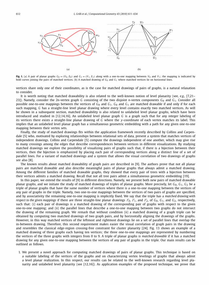
Fig. 6. Illustration of subcase BT in which the two sides of (e) that intersect all unused y-coordinates are both incident on v j : (a) A safe region (e) ofthe edge e = (v j , vk). (b) Addition of the vertex vi having label B . (c) Addition of the vertex vi having label T .
Details on the steps of the drawing algorithm are given below.
Step 0 and step 1. The x-coordinate of both vertices v0 and v1 is set to 0. If both v0 and v1 have label B , then they areassigned y-coordinates 0 and 1, respectively. If they both have label T , then they are assigned y-coordinates n − 2and n − 1, respectively. Otherwise (v0 and v1 have distinct BT-labels), the vertex with label B is given y-coordinate 0,while the other is given y-coordinate n −1. Depending on the different cases, the safe region (e) of edge e = (v0, v1)
is defined as in Fig. 4.Step i (2 � i � n − 1). The addition of vi makes a new face in the drawing. This face consists of two edges incident to vi
and one of the candidate edges of Γ0(i − 1). Let e = (v j, vk) be such a candidate edge of Γ0(i − 1) ( j,k < i and j = k).Let (e) be a safe region of e and let p be the corner of (e) other than v j and vk . Vertex vi is drawn inside (e).There are four cases to be considered.• Case BB: both v j and vk have label B. See Fig. 5. If vi is labeled B , then it is drawn at the minimum unused y-coordinate
(see, e.g., Fig. 5(b)). Otherwise, it is drawn at the maximum unused y-coordinate (see, e.g., Fig. 5(c)).If edge (v j, vi) is a candidate edge of Γ0(i), then its safe region is defined as the open triangle (v j, vi, p). Similarly,if (vk, vi) is a candidate edge of Γ0(i), then its safe region is the open triangle (vk, vi, p).
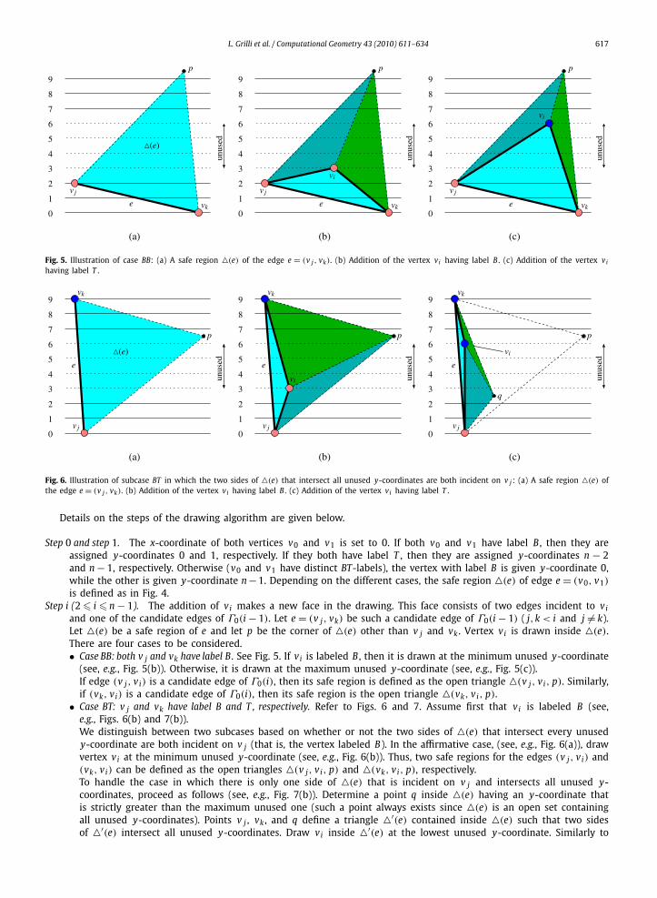
• Case BT: v j and vk have label B and T , respectively. Refer to Figs. 6 and 7. Assume first that vi is labeled B (see,e.g., Figs. 6(b) and 7(b)).We distinguish between two subcases based on whether or not the two sides of (e) that intersect every unusedy-coordinate are both incident on v j (that is, the vertex labeled B). In the affirmative case, (see, e.g., Fig. 6(a)), drawvertex vi at the minimum unused y-coordinate (see, e.g., Fig. 6(b)). Thus, two safe regions for the edges (v j, vi) and(vk, vi) can be defined as the open triangles (v j, vi, p) and (vk, vi, p), respectively.To handle the case in which there is only one side of (e) that is incident on v j and intersects all unused y-coordinates, proceed as follows (see, e.g., Fig. 7(b)). Determine a point q inside (e) having an y-coordinate thatis strictly greater than the maximum unused one (such a point always exists since (e) is an open set containingall unused y-coordinates). Points v j , vk , and q define a triangle ′(e) contained inside (e) such that two sidesof ′(e) intersect all unused y-coordinates. Draw vi inside ′(e) at the lowest unused y-coordinate. Similarly to

618 L. Grilli et al. / Computational Geometry 43 (2010) 611–634
Fig. 7. Illustration of subcase BT in which the two sides of (e) that intersect all unused y-coordinates are both incident on vk : (a) A safe region (e) ofthe edge e = (v j , vk). (b) Addition of the vertex vi having label B . (c) Addition of the vertex vi having label T .
the previous case, the open triangles (v j, vi,q) and (vi, vk,q) define two safe regions for the edges (v j, vi) and(vk, vi), respectively.The case when vi is labeled T is symmetric to the case when vi is labeled B (see, e.g., Figs. 6(c) and 7(c)).
• Case TB: v j and vk have label T and B, respectively. This case is symmetric to the case BT .• Case TT: both v j and vk have label T . This case is symmetric to the case BB.
End Algorithm BT-Draw-Outerplane
Lemma 1. Let G0 be a maximal outerplane graph with n vertices and a given BT-labeling. Algorithm BT-Draw-Outerplanecomputes in O (n) time a BT-label preserving straight-line planar drawing of G0 .
Proof. We first prove that Algorithm BT-Draw-Outerplane maintains the invariants, which implies that by constructionevery vertex labeled B has an y-coordinate smaller than the y-coordinate of any vertex labeled T . Then we show that thecomputed drawing is planar and finally we discuss the time complexity.
The invariants are trivially true at the end of step 1. Assume that invariants I1 and I2 hold at the end of step i − 1(2 � i � n − 1). The addition of vi and of the two edges (v j, vi) and (vk, vi) changes the set of the candidate edges of Γ0(i)with respect to those of Γ0(i − 1). Namely, edge (vk, v j) is no longer a candidate edge while all other candidate edges ofΓ0(i − 1) remain candidate edges of Γ0(i). Let f be the face of G0 whose vertices are vk , v j , vi . Of course, if f correspondsto a leaf node of G∗
0, then the set of candidate edges of Γ0(i) is the same as that of Γ0(i − 1) without the edge (vk, v j).Therefore, invariants I1 and I2 are maintained since the safe regions of the candidate edges of Γ0(i) still remain those ofthe candidate edges of Γ0(i − 1). On the other hand, if f corresponds to a non-leaf node in the weak dual G∗
0, then at leastone of (v j, vi) and (vk, vi) is a new candidate edge of Γ0(i). By construction, the safe regions of these two edges existand are contained inside the safe region of edge (v j, vk) which, by inductive hypothesis, does not intersect the safe regionsof the other candidate edges of Γ0(i − 1). Hence, the safe regions of (v j, vi) and (vk, vi) do not intersect the safe regionsof the other candidate edges; furthermore, they do not intersect each other. It follows that both invariants I1 and I2 aremaintained at the end of step i.
As for the planarity of the computed drawing, note that Γ0(1) is planar because it consists of an edge. Suppose that byinduction Γ0(i − 1) is planar for some 2 � i � n − 1. Since vi is drawn in a safe region which, by definition, has an emptyintersection with Γ0(i − 1), it follows that the addition of vi and of the two straight-line edges incident to vi introducesneither edge crossings nor vertex-edge overlaps. Hence, Γ0(i) is also planar.
Finally, the dual of the outerplane graph can be constructed and visited in O (n) time. The drawing is computed by usinga vertex addition strategy. The algorithm spends O (1) time to draw each vertex and its incident edges. The incrementalstrategy never changes the location of the drawing computed at previous steps. It follows that Algorithm BT-Draw-Outerplane runs in O (n) time. �3.1.3. Matching phase
In this phase, we complete the construction of a matched drawing of the pair 〈G0, G1〉, with respect to the given one-to-one mapping, by computing a (BT-label preserving) straight-line planar drawing Γ1 of G1 whose vertices have the samey-coordinates as those of the corresponding vertices of G0. Our strategy for computing Γ1 consists of three steps. First, weremove from G1 the faces corresponding to the leaves of G∗
1, in order to obtain an outerpath having the spine of G∗1 as
weak dual. Then, we compute a (level preserving) drawing of this outerpath and finally, we reinsert the pruned faces of G1in the computed drawing.
L. Grilli et al. / Computational Geometry 43 (2010) 611–634 619
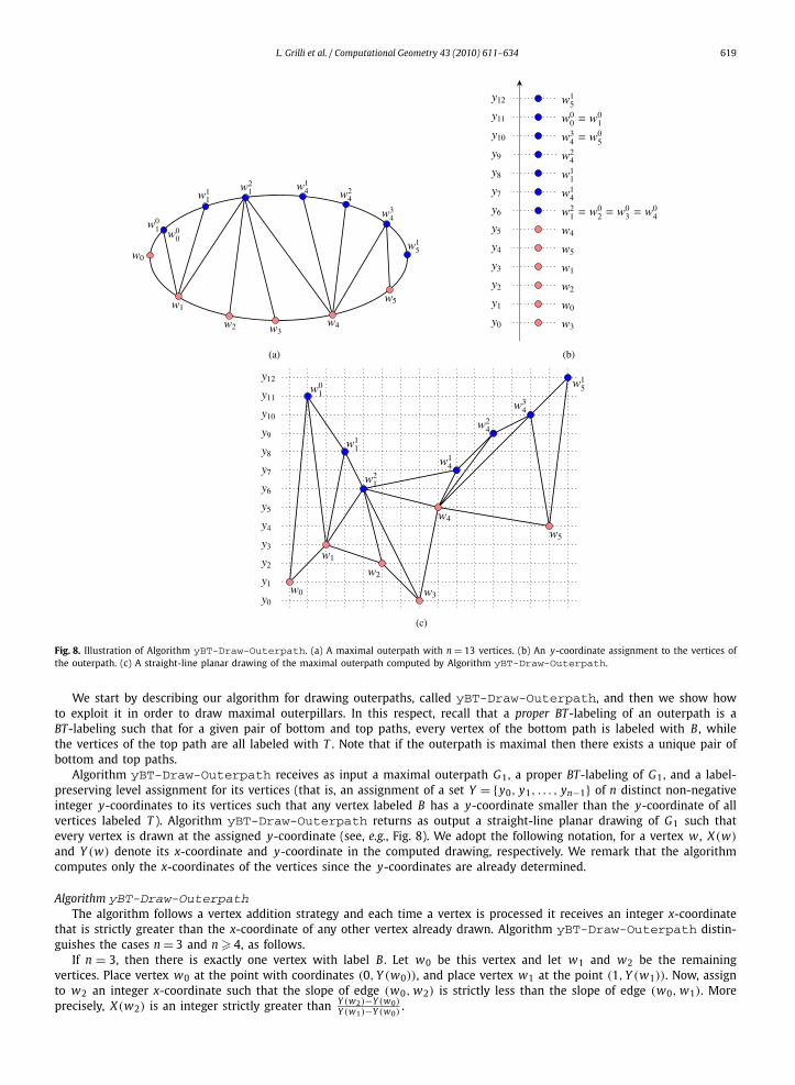
Fig. 8. Illustration of Algorithm yBT-Draw-Outerpath. (a) A maximal outerpath with n = 13 vertices. (b) An y-coordinate assignment to the vertices ofthe outerpath. (c) A straight-line planar drawing of the maximal outerpath computed by Algorithm yBT-Draw-Outerpath.
We start by describing our algorithm for drawing outerpaths, called yBT-Draw-Outerpath, and then we show howto exploit it in order to draw maximal outerpillars. In this respect, recall that a proper BT-labeling of an outerpath is aBT-labeling such that for a given pair of bottom and top paths, every vertex of the bottom path is labeled with B , whilethe vertices of the top path are all labeled with T . Note that if the outerpath is maximal then there exists a unique pair ofbottom and top paths.
Algorithm yBT-Draw-Outerpath receives as input a maximal outerpath G1, a proper BT-labeling of G1, and a label-preserving level assignment for its vertices (that is, an assignment of a set Y = {y0, y1, . . . , yn−1} of n distinct non-negativeinteger y-coordinates to its vertices such that any vertex labeled B has a y-coordinate smaller than the y-coordinate of allvertices labeled T ). Algorithm yBT-Draw-Outerpath returns as output a straight-line planar drawing of G1 such thatevery vertex is drawn at the assigned y-coordinate (see, e.g., Fig. 8). We adopt the following notation, for a vertex w , X(w)
and Y (w) denote its x-coordinate and y-coordinate in the computed drawing, respectively. We remark that the algorithmcomputes only the x-coordinates of the vertices since the y-coordinates are already determined.
Algorithm yBT-Draw-OuterpathThe algorithm follows a vertex addition strategy and each time a vertex is processed it receives an integer x-coordinate
that is strictly greater than the x-coordinate of any other vertex already drawn. Algorithm yBT-Draw-Outerpath distin-guishes the cases n = 3 and n � 4, as follows.
If n = 3, then there is exactly one vertex with label B . Let w0 be this vertex and let w1 and w2 be the remainingvertices. Place vertex w0 at the point with coordinates (0, Y (w0)), and place vertex w1 at the point (1, Y (w1)). Now, assignto w2 an integer x-coordinate such that the slope of edge (w0, w2) is strictly less than the slope of edge (w0, w1). Moreprecisely, X(w2) is an integer strictly greater than Y (w2)−Y (w0) .
Y (w1)−Y (w0)
620 L. Grilli et al. / Computational Geometry 43 (2010) 611–634
If n � 4, consider the bottom path Πb of G1 and let nb be the size of Πb . A straight-line planar drawing of G1 thatpreserves the given y-coordinates is computed in nb steps. Visit Πb from its source to its sink and denote as wk the kthencountered vertex starting from 0 (see, e.g., Fig. 8(a)). At step i, vertex wi ∈ Πb and its neighbors in the top path that arenot yet drawn are processed. If wi has d(i) neighbors in Πt , then denote these neighbors as w j
i , j ∈ {0,1, . . . ,d(i) − 1},according to their ordering in the top path. The algorithm proceeds as follows.
At step 0, vertex w0 is drawn at the point (0, Y (w0)). Notice that, w0 has exactly one neighbor w00 in the top path.
Draw vertex w00 at point (1, Y (w0
0)).At step i (1 � i � nb − 1), vertex wi is the apex of a fan that contains one or more vertices of Πt . Furthermore, since
all internal faces of G1 are three-cycles and always contain two vertices with distinct labels, the first neighbor of wi inΠt coincides with the last neighbor of wi−1 in Πt , that is w0
i = wd(i)−1i−1 . Hence, vertex w0
i has been already drawn atsome previous step. In order to draw wi while preserving the planar embedding of G1, we distinguish two cases based onwhether the slope of the edge (w0
i , wi−1) is positive. In the affirmative case, vertex wi is drawn at point (X(w0i )+1, Y (wi)).
In the negative case, wi is given an integer x-coordinate such that the edges (w0i , wi−1) and (w0
i , wi) have increasing (i.e.,
less negative) slopes. Namely, X(wi) is an integer strictly greater thanY (wi)−Y (w0
i )
Y (wi−1)−Y (w0i )
[X(wi−1) − X(w0i )] + X(w0
i ). Now, if
d(i) � 2, then vertex w1i is drawn at point (X(wi) + 1, Y (w1
i )) and vertices w2i , . . . , wd(i)−1
i are given suitable integer x-
coordinates so that their incident edges (wi, w ji ) have decreasing (i.e., less positive) slopes. Namely, X(w j
i ) (2 � j � d(i)−1)
is an integer strictly greater than
Y (w ji ) − Y (wi)
Y (w j−1i ) − Y (wi)
[X(
w j−1i
) − X(wi)] + X(wi).
End Algorithm yBT-Draw-Outerpath
Lemma 2. Let G1 be an outerpath with n vertices and a proper BT-labeling. For any label-preserving level assignment, AlgorithmyBT-Draw-Outerpath computes in O (n) time a straight-line planar drawing of G1 where every vertex is given an y-coordinateequal to its level number.
Proof. We first show that the computed drawing is planar and then discuss the time complexity of the algorithm.By construction, each vertex of the computed drawing has an assigned y-coordinate, and edges connecting a vertex of
the bottom path with a vertex of the top path cannot cross each other. Also, the top and bottom paths are drawn as twostrictly x-monotone chains with the top path entirely above the bottom path, thus their edges cannot intersect each other.Therefore, crossings may occur only between an edge joining the top and bottom paths and an edge of one of these paths.
More precisely, let (wi, wi+1) be an edge of Πb and let (wk, w jk) be an edge between a vertex wk ∈ Πb and a vertex
w jk ∈ Πt .
• If k < i, then wk and w jk are both to the left of wi and of wi+1, hence these edges are represented by two disjoint
segments.• If k = i, then edges (wi, wi+1) and (wi, w j
i ) share the vertex wi and they cannot overlap. More precisely, if X(w ji ) <
X(wi), then w ji − wi − wi+1 is a strictly x-monotone chain. On the other hand, if X(w j
i ) > X(wi), the segment wi w ji
has a positive slope that is strictly greater than the slope of the segment wi wi+1 since Y (w ji ) > Y (wi+1) and, by
construction, X(w ji ) < X(wi+1).
• Similarly, if k = i + 1, then edges (wi, wi+1) and (wi+1, w ji+1) share the vertex wi+1. They cannot overlap if X(w j
i+1) >
X(wi). On the other hand, if X(w ji+1) < X(wi), then j = 0 and w0
i+1 = w0i . In this case, vertices w0
i , wi and wi+1
cannot be collinear because, by construction, segments w0i wi and w0
i wi+1 have increasing (negative) slopes.
• Consider now the case in which k > i + 1. We distinguish two subcases based on whether X(w jk) > X(wi+1). In the
affirmative case, vertices wk and w jk are both to the right of wi+1, and thus, edges (wi, wi+1) and (wk, w j
k) are
represented by two disjoint segments. In the negative case, (that is X(w jk) < X(wi+1)) j must be equal to 0 and w0
kcoincides with w0
i+1, and thus, edges (wi, wi+1) and (wk, w0k ) cannot intersect because, by construction, the segment
w0k wi+1 has a negative slope that is strictly smaller than the (negative) slope of the segment w0
k wk .
By a symmetric argument, it can be proved that an edge of the top path and an edge joining a vertex of the top path witha vertex of the bottom path cannot intersect. From which follows that the computed drawing is planar.
Concerning the time complexity, note that Algorithm yBT-Draw-Outerpath follows a vertex addition strategy andprocesses vertices one at a time. Each vertex and its incident edges require O (1) time to be drawn, because only a constantnumber of algebraic operations must be executed. It follows that yBT-Draw-Outerpath runs in O (n) time. �
L. Grilli et al. / Computational Geometry 43 (2010) 611–634 621
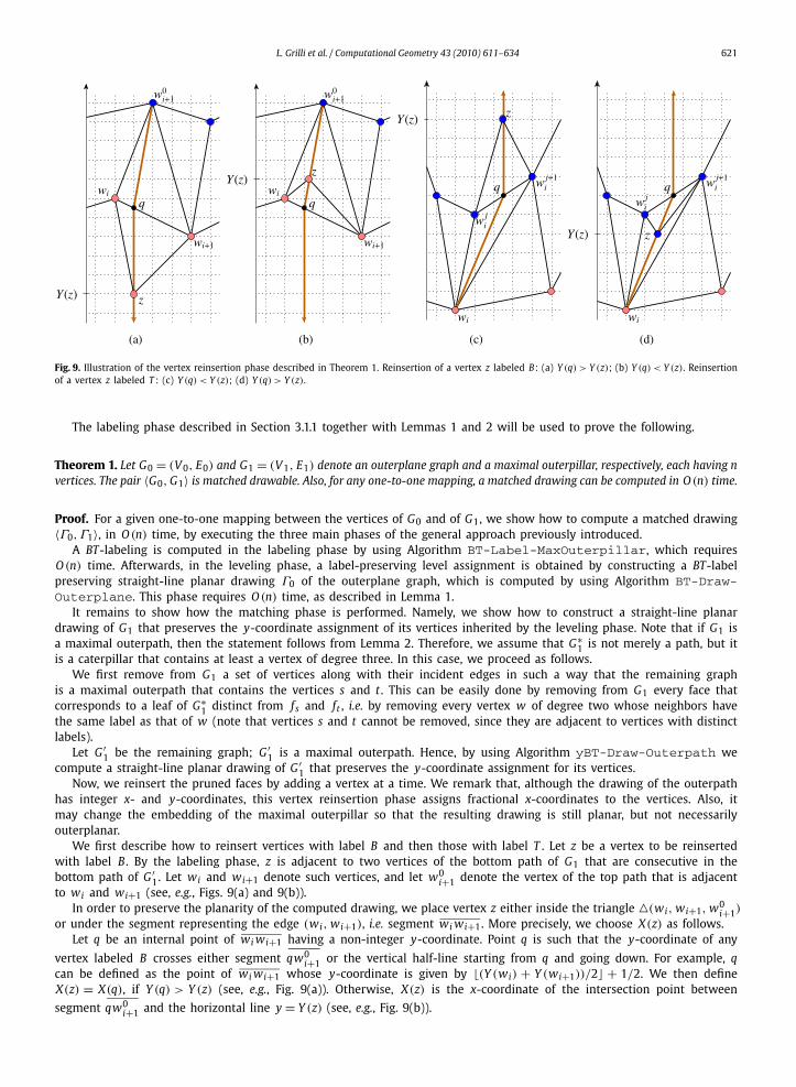
Fig. 9. Illustration of the vertex reinsertion phase described in Theorem 1. Reinsertion of a vertex z labeled B: (a) Y (q) > Y (z); (b) Y (q) < Y (z). Reinsertionof a vertex z labeled T : (c) Y (q) < Y (z); (d) Y (q) > Y (z).
The labeling phase described in Section 3.1.1 together with Lemmas 1 and 2 will be used to prove the following.
Theorem 1. Let G0 = (V 0, E0) and G1 = (V 1, E1) denote an outerplane graph and a maximal outerpillar, respectively, each having nvertices. The pair 〈G0, G1〉 is matched drawable. Also, for any one-to-one mapping, a matched drawing can be computed in O (n) time.
Proof. For a given one-to-one mapping between the vertices of G0 and of G1, we show how to compute a matched drawing〈Γ0,Γ1〉, in O (n) time, by executing the three main phases of the general approach previously introduced.
A BT-labeling is computed in the labeling phase by using Algorithm BT-Label-MaxOuterpillar, which requiresO (n) time. Afterwards, in the leveling phase, a label-preserving level assignment is obtained by constructing a BT-labelpreserving straight-line planar drawing Γ0 of the outerplane graph, which is computed by using Algorithm BT-Draw-Outerplane. This phase requires O (n) time, as described in Lemma 1.
It remains to show how the matching phase is performed. Namely, we show how to construct a straight-line planardrawing of G1 that preserves the y-coordinate assignment of its vertices inherited by the leveling phase. Note that if G1 isa maximal outerpath, then the statement follows from Lemma 2. Therefore, we assume that G∗
1 is not merely a path, but itis a caterpillar that contains at least a vertex of degree three. In this case, we proceed as follows.
We first remove from G1 a set of vertices along with their incident edges in such a way that the remaining graphis a maximal outerpath that contains the vertices s and t . This can be easily done by removing from G1 every face thatcorresponds to a leaf of G∗
1 distinct from f s and ft , i.e. by removing every vertex w of degree two whose neighbors havethe same label as that of w (note that vertices s and t cannot be removed, since they are adjacent to vertices with distinctlabels).
Let G ′1 be the remaining graph; G ′
1 is a maximal outerpath. Hence, by using Algorithm yBT-Draw-Outerpath wecompute a straight-line planar drawing of G ′
1 that preserves the y-coordinate assignment for its vertices.Now, we reinsert the pruned faces by adding a vertex at a time. We remark that, although the drawing of the outerpath
has integer x- and y-coordinates, this vertex reinsertion phase assigns fractional x-coordinates to the vertices. Also, itmay change the embedding of the maximal outerpillar so that the resulting drawing is still planar, but not necessarilyouterplanar.
We first describe how to reinsert vertices with label B and then those with label T . Let z be a vertex to be reinsertedwith label B . By the labeling phase, z is adjacent to two vertices of the bottom path of G1 that are consecutive in thebottom path of G ′
1. Let wi and wi+1 denote such vertices, and let w0i+1 denote the vertex of the top path that is adjacent
to wi and wi+1 (see, e.g., Figs. 9(a) and 9(b)).In order to preserve the planarity of the computed drawing, we place vertex z either inside the triangle (wi, wi+1, w0
i+1)
or under the segment representing the edge (wi, wi+1), i.e. segment wi wi+1. More precisely, we choose X(z) as follows.Let q be an internal point of wi wi+1 having a non-integer y-coordinate. Point q is such that the y-coordinate of any
vertex labeled B crosses either segment qw0i+1 or the vertical half-line starting from q and going down. For example, q
can be defined as the point of wi wi+1 whose y-coordinate is given by �(Y (wi) + Y (wi+1))/2� + 1/2. We then defineX(z) = X(q), if Y (q) > Y (z) (see, e.g., Fig. 9(a)). Otherwise, X(z) is the x-coordinate of the intersection point between
segment qw0 and the horizontal line y = Y (z) (see, e.g., Fig. 9(b)).
i+1
622 L. Grilli et al. / Computational Geometry 43 (2010) 611–634
Fig. 10. (a) K3 edge. (b) C4 edge. (c) K +3 edge. (d) C+
4 edge. (e) Kite edge. (f) Outerpath. (g) Generalized outerpath.
Similarly, suppose now that z is labeled T , and let w ji and w j+1
i be its neighbors, where wi is the vertex of the bottom
path that is adjacent to both vertices w ji and w j+1
i . Choose a point q of segment w ji w j+1
i with a non-integer coordinate.Draw z at point (X(q), Y (z)), if Y (q) < Y (z) (see, e.g., Fig. 9(c)). Otherwise, place z at the intersection point between thesegment qwi and the horizontal line y = Y (z) (see, e.g., Fig. 9(d)).
Concerning the time complexity, we observe that the maximal outerpath can be extracted from the maximal outerpillarin linear time, since it can be obtained by removing the faces of G1 corresponding to the leaves of G∗
1 that are distinctfrom f s and ft . Furthermore, in the vertex reinsertion phase, each vertex z together with its incident edges are added tothe drawing one at a time and X(z) is always computed with a constant number of algebraic operations. Therefore, thematching phase requires linear time and the overall time complexity is O (n). �3.2. Matched drawing of 〈outerplane, generalized outerpath〉
In this section, we introduce a new family of graphs that include the maximal outerpillars as a special case and extendthe result of Theorem 1 to the graph pairs consisting of an outerplane graph and a graph of this family. We adopt someterminology from [16].
(a) A K3 edge is the cycle u − v − w − u on vertices {u, v, w} (see Fig. 10(a)).(b) A C4 edge is the cycle u − s − v − t − u on vertices {u, v, s, t} (see Fig. 10(b)).(c) A K +
3 edge is set of cycles u − v − w ′ − u with edge (u, v) on vertices {u, v} ∪ W , where w ′ ∈ W for some non-emptyvertex set W (see Fig. 10(c)).
(d) A C+4 edge is set of cycles u − w − v − w ′ − u on vertices {u, v, w} ∪ W , where w ′ ∈ W for some non-empty vertex set
W (see Fig. 10(d)).(e) A kite edge is the cycle u − s − v − t − u with edge (s, t) on vertices {u, v, s, t} (see Fig. 10(e)).
Let O be an outerpath (that is an outerpillar whose weak dual is a path) and let G be a graph obtained from O by replacingsome edges of the external face of O with a K +
3 edge, a C+4 edge, or a kite edge. Graph G is called a generalized outerpath.
For example, Fig. 10(f) shows an outerpath O and Fig. 10(g) shows a generalized outerpath G; in the figure, edge (u′, v ′)of O has been replaced by a C+
4 edge in G . Notice that a maximal outerpillar is a generalized outerpath obtained from amaximal outerpath by using only K3 edges.
A slightly involved but quite straightforward extension of the drawing technique described in Section 3.1 implies thefollowing theorem. The interested reader can find its proof in Appendix A.
Theorem 2. Let G0 = (V 0, E0) and G1 = (V 1, E1) denote an outerplane graph and a generalized outerpath, respectively, each havingn vertices. The pair 〈G0, G1〉 is matched drawable. Also, for any one-to-one mapping, a matched drawing of 〈G0, G1〉 can be computedin O (n) time.
L. Grilli et al. / Computational Geometry 43 (2010) 611–634 623
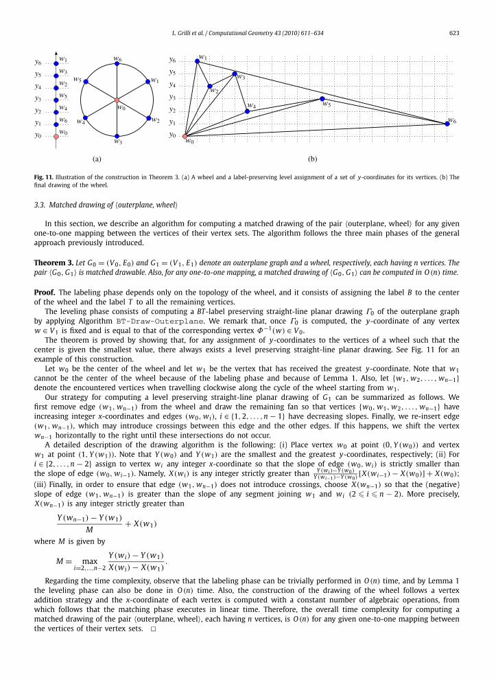
Fig. 11. Illustration of the construction in Theorem 3. (a) A wheel and a label-preserving level assignment of a set of y-coordinates for its vertices. (b) Thefinal drawing of the wheel.
3.3. Matched drawing of 〈outerplane, wheel〉
In this section, we describe an algorithm for computing a matched drawing of the pair 〈outerplane, wheel〉 for any givenone-to-one mapping between the vertices of their vertex sets. The algorithm follows the three main phases of the generalapproach previously introduced.
Theorem 3. Let G0 = (V 0, E0) and G1 = (V 1, E1) denote an outerplane graph and a wheel, respectively, each having n vertices. Thepair 〈G0, G1〉 is matched drawable. Also, for any one-to-one mapping, a matched drawing of 〈G0, G1〉 can be computed in O (n) time.
Proof. The labeling phase depends only on the topology of the wheel, and it consists of assigning the label B to the centerof the wheel and the label T to all the remaining vertices.
The leveling phase consists of computing a BT-label preserving straight-line planar drawing Γ0 of the outerplane graphby applying Algorithm BT-Draw-Outerplane. We remark that, once Γ0 is computed, the y-coordinate of any vertexw ∈ V 1 is fixed and is equal to that of the corresponding vertex Φ−1(w) ∈ V 0.
The theorem is proved by showing that, for any assignment of y-coordinates to the vertices of a wheel such that thecenter is given the smallest value, there always exists a level preserving straight-line planar drawing. See Fig. 11 for anexample of this construction.
Let w0 be the center of the wheel and let w1 be the vertex that has received the greatest y-coordinate. Note that w1cannot be the center of the wheel because of the labeling phase and because of Lemma 1. Also, let {w1, w2, . . . , wn−1}denote the encountered vertices when travelling clockwise along the cycle of the wheel starting from w1.
Our strategy for computing a level preserving straight-line planar drawing of G1 can be summarized as follows. Wefirst remove edge (w1, wn−1) from the wheel and draw the remaining fan so that vertices {w0, w1, w2, . . . , wn−1} haveincreasing integer x-coordinates and edges (w0, wi), i ∈ {1,2, . . . ,n − 1} have decreasing slopes. Finally, we re-insert edge(w1, wn−1), which may introduce crossings between this edge and the other edges. If this happens, we shift the vertexwn−1 horizontally to the right until these intersections do not occur.
A detailed description of the drawing algorithm is the following: (i) Place vertex w0 at point (0, Y (w0)) and vertexw1 at point (1, Y (w1)). Note that Y (w0) and Y (w1) are the smallest and the greatest y-coordinates, respectively; (ii) Fori ∈ {2, . . . ,n − 2} assign to vertex wi any integer x-coordinate so that the slope of edge (w0, wi) is strictly smaller thanthe slope of edge (w0, wi−1). Namely, X(wi) is any integer strictly greater than Y (wi)−Y (w0)
Y (wi−1)−Y (w0)[X(wi−1) − X(w0)] + X(w0);
(iii) Finally, in order to ensure that edge (w1, wn−1) does not introduce crossings, choose X(wn−1) so that the (negative)slope of edge (w1, wn−1) is greater than the slope of any segment joining w1 and wi (2 � i � n − 2). More precisely,X(wn−1) is any integer strictly greater than
Y (wn−1) − Y (w1)
M+ X(w1)
where M is given by
M = maxi=2,...,n−2
Y (wi) − Y (w1)
X(wi) − X(w1).
Regarding the time complexity, observe that the labeling phase can be trivially performed in O (n) time, and by Lemma 1the leveling phase can also be done in O (n) time. Also, the construction of the drawing of the wheel follows a vertexaddition strategy and the x-coordinate of each vertex is computed with a constant number of algebraic operations, fromwhich follows that the matching phase executes in linear time. Therefore, the overall time complexity for computing amatched drawing of the pair 〈outerplane, wheel〉, each having n vertices, is O (n) for any given one-to-one mapping betweenthe vertices of their vertex sets. �

624 L. Grilli et al. / Computational Geometry 43 (2010) 611–634
Fig. 12. Construction of the drawing Γ0. (a) Wheels do not have matched centers. (b) Wheels have matched centers.
3.4. Matched drawing of 〈wheel, wheel〉
In this section, we show how to construct a matched drawing of two wheels for any given one-to-one mapping betweenthe vertices of their vertex sets. The algorithm is described in the proof of the following theorem and follows the high leveldescription introduced at the beginning of this section.
Theorem 4. Let G0 = (V 0, E0) and G1 = (V 1, E1) denote two wheels, each having n vertices. The pair 〈G0, G1〉 is matched drawable.Also, for any one-to-one mapping, a matched drawing of 〈G0, G1〉 can be computed in O (n) time.
Proof. The labeling phase is the same as in the proof of Theorem 3, that is, the center of G1 is labeled B , and all othervertices are labeled T .
The leveling phase is executed by computing a straight-line planar drawing Γ0 of G0 such that the y-coordinates of thevertices of Γ0 define a label-preserving level assignment. This drawing is computed by distinguishing two cases: either thecenter of G0 is matched to the center of G1, or it is matched to some other vertex of G1. In both cases, we denote as C0the cycle of the wheel, that is obtained after the removal of its center.
Consider first the case that the two centers are not matched. We show how to construct Γ0 in O (n) time on an n × ngrid. Let v0 be the vertex of G0 that corresponds to the center of G1, i.e. Φ(v0) is the center of G1, and let v1 be thecenter of G0. Also, let {v2, v3, . . . , vn−1} be the sequence of vertices that are encountered when traversing the cycle C0clockwise starting at vertex v0 (see Fig. 12(a)). Draw vertex v0 at point (0,0) and draw vertex v1 at point (1,1). Now, fori ∈ {2,3, . . . ,n − 1} draw vertex vi at point (i,n − i + 1). By construction, the resulting drawing Γ0 preserves the BT-labeling.Furthermore, Γ0 is planar and its construction requires O (n) time.
Now consider the case that the centers of the wheels are matched, and let v0 be the center of G0. We construct Γ0in O (n) time on an (n + 1) × n grid as follows. See Fig. 12(b). Let {v1, v2, . . . , vn−1} be the sequence of vertices that areencountered when traversing the cycle of C0 clockwise starting at any vertex v1. Draw vertex v0 at point (0,0), and fori ∈ {1,2, . . . ,n − 2} draw vertex vi at point (i,n − i). Finally, in order to avoid collinearities between edge (v1, vn−1) andedges in the path v1 − v2 − · · · − vn−1, draw vertex vn−1 at point (n + 1,1). It is immediate to see that Γ0 preserves theBT-labeling, is planar, and can be computed in O (n) time.
The matching phase consists of computing a drawing of G1 as described in the proof of Theorem 3.Finally, taking into account the previous considerations on the time complexity and by an argument similar to that of the
proof of Theorem 3, it follows that the overall time complexity for computing a matched drawing of two n-vertex wheels isO (n), for any given one-to-one mapping. �4. Matched drawings of graph triples
In this section, we extend the definition of matched drawing in order to allow the pairwise comparison of three n-vertexplanar graphs.
Note that any number of unlabeled level planar graphs have a matched drawing such that matched vertices have thesame y-coordinate. It can be trivially constructed by horizontally aligning the drawings of the graphs. However, in thistype of visualization, matched vertices of two non-consecutively aligned drawings lie on a set of parallel lines that wouldoverlap the in-between representations. Similarly to the classical edge-region crossing-free requirement of cluster planarity(see [24]) we add the constraint that the lines describing the matching of a pair of graphs never intersect the area occupiedby the drawing of the third graph.
Let G0 = (V 0, E0), G1 = (V 1, E1) and G2 = (V 2, E2) be a triple of planar graphs such that |V 0| = |V 1| = |V 2| = n. LetΦ01 : V 0 → V 1 and Φ12 : V 1 → V 2 be two one-to-one mappings between the vertices of the pairs 〈G0, G1〉 and 〈G1, G2〉,respectively. Let Φ20 : V 2 → V 0 denote the one-to-one mapping that is implicitly fixed by associativity from the mappingsΦ01 and Φ12, i.e. Φ20 = (Φ01 ◦ Φ12)
−1. Let Γ0, Γ1 and Γ2 be three straight-line planar drawings of G0, G1 and G2, respec-tively. The triple of drawings 〈Γ0,Γ1,Γ2〉 is a matched drawing of G0, G1 and G2, with respect to the mappings Φ01,Φ12 and

L. Grilli et al. / Computational Geometry 43 (2010) 611–634 625
Φ20, if for all i ∈ {0,1,2} the following requirements hold: (1) Each pair of drawings 〈Γi,Γ(i+1) mod 3〉 is a matched drawingof the corresponding graph pairs 〈Gi, G(i+1) mod 3〉 with respect to the one-to-one mapping Φi(i+1) mod 3; and (2) Let Lidenote the set of parallel lines of the one-to-one mapping Φi(i+1) mod 3, then Li ∩ Γ(i+2) mod 3 = ∅. Namely, the parallellines of any one-to-one mapping between two graphs do not intersect with the drawing of the remaining graph. A tripleof planar graph is matched drawable if it has a matched drawing for any given one-to-one mapping between the vertices ofany pair of graphs in the triple.
In [19], it was proved that there exist two trees that do not admit a simultaneous geometric embedding, while in [9],it was proved that every pair of trees is matched drawable. The next theorem contributes by shedding more light on thedifferences between the notion of matched drawability and simultaneous drawability. Namely, while it is known that triplesof graphs with the same vertex set may not have a simultaneous geometric embedding even in the case that they are simplepaths [2], it turns out that a triple consisting of a caterpillar and two unlabeled level planar graphs is matched drawable.We remark that, trees that are ULP graphs are characterized in [12]; general unlabeled level planar graphs are characterizedin [16] as follows.
Lemma 3. (See [16].) A planar graph is ULP if and only if it is either a generalized caterpillar, or a radius-2 star, or an extended degree-3spider.
4.1. Matched drawings of a caterpillar and two unlabeled level planar graphs
Before describing the main result of this section, we give a technical lemma and introduce a suitable ordering of thevertices of a caterpillar that are needed to prove this result.
Let Γ be a straight-line planar drawing, and let v be a vertex of Γ . A safe region for v is a disk centered at v , anddenoted as SR(v), such that, if Γ is perturbed by moving v to any point inside SR(v), the modified drawing stays planar.The following lemma shows how to compute SR(v) for a vertex v of a given straight-line planar drawing Γ . SR(v) isobtained by looking only at the pairs of elements (vertices of edges) in Γ that are not incident with each other. That is, thelemma considers pairs of elements in Γ whose relative distance is strictly greater than zero.
Lemma 4. Let Γ be a straight-line planar drawing, and let v be a vertex of Γ . Let δΓ be the minimum non-zero distance between anypair of elements (vertices or edges) of Γ . Then, a disk centered at vertex v and having radius r < δΓ is a safe region for v.
Proof. Suppose that vertex v is moved from its initial position, at point P , to a new position, at point P ′ , inside the saferegion; hence d(P , P ′) � r < δΓ . Of course, vertex v cannot overlap any other vertex or edge of Γ . Therefore, possiblecrossings may occur only between an edge e incident on v and any other element of Γ , namely a vertex distinct from v ,or an edge that is not incident on v .
Suppose, for contradiction, that there is a crossing between an edge e incident to v and an element o of Γ . This wouldimply that edge e has been moved towards element o by an amount δeo greater or equal to their initial distance, thus δeo �δΓ . However, δeo cannot be greater than d(P , P ′), i.e. d(P , P ′) � δeo , and thus d(P , P ′) � δΓ , which is a contradiction. �
Let G and S denote a caterpillar and its spine, respectively. Let s and t be the end-vertices of the spine. Orient the spinefrom s to t . A spine-monotone ordering associates each vertex v of G with a distinct non-negative integer ord v according tothe following rules:
(i) vertex s is given number 0, that is ord s = 0;(ii) for any pair of distinct vertices u, v of S such that u precedes v , we have ord u < ord v;
(iii) for any edge (u, w) such that w is a leaf and u is not, we have ord u < ord w;(iv) for any three vertices u, v, w such that u and v belong to S , u precedes v along S , and w is a leaf adjacent to u, we
have ord u < ord w < ord v .
Note that a spine-monotone ordering of G can be easily obtained by a suitable traversal of G starting with s and such thatfor each visited vertex v , the vertices adjacent to v with degree 1 are visited before those having degree greater than 1.
Theorem 5. Let G0 = (V 0, E0) be an n-vertex caterpillar, and let G1 = (V 1, E1) and G2 = (V 2, E2) be two n-vertex unlabeled levelplanar graphs. The triple 〈G0, G1, G2〉 is matched drawable. Also, for any one-to-one mapping, a matched drawing of 〈G0, G1, G2〉 canbe computed in O (n3) time.
Proof. Compute a spine-monotone ordering of G0. Denote each vertex v of G0 as the integer j (0 � j � n − 1) such thatj = ord v . Let L0 = {l0 j: 0 � j � n − 1} be a set of parallel horizontal lines, where l0 j = {(x, j): x ∈ R}. Assign vertex j of G0to line l0 j . For an example, see Fig. 13.
Since G1 is an ULP graph, there exists a straight-line planar drawing Γ1 of G1 preserving the vertex numbering definedby L0 [16] and the mapping Φ01. Define L1 as a set of parallel lines with slope α different from that of L0 and such that
626 L. Grilli et al. / Computational Geometry 43 (2010) 611–634
Fig. 13. Matched drawing of three caterpillars. The numbering of the vertices of G0 is a spine-monotone numbering.
each line of L1 passes through a distinct vertex of Γ1. The value of α can be chosen as any angle in the interval [π/6,π/3]that is distinct from the slopes of all the lines through any pair of vertices of Γ1. Note that the lines of L1 may not beuniformly spaced. Similarly, there exists a straight-line planar drawing Γ2 of G2 preserving the vertex numbering definedby L1 and the mapping Φ12. Also, define L2 as a set of parallel lines such that each line of L2 passes only through a distinctvertex of Γ2. Fig. 13 shows an example of three possible sets of parallel lines L0, L1 and L2, where the lines in each set areuniformly spaced.
The intersections of the lines L2 with those of L0 completely define a drawing Γ0 of G0, i.e. each vertex v ∈ V 0 is drawnat the intersection point of its corresponding lines l0v ∈ L0 and l2v ∈ L2. By construction, the y-coordinates of Γ0 definea spine-monotone ordering of G0. This implies that any pair of edges of Γ0 with no vertex in common cannot cross eachother. More precisely, let e = (u, w) and e′ = (v, z) be two edges of Γ0 with distinct end-vertices. It is immediate to see thate and e′ are disjoint if at least one of them is an edge of the spine of G0. Otherwise, both edges are incident exactly to onevertex of the spine; without loss of generality suppose that u and v are vertices of the spine of G0 such that u precedes v .By the rule (iv) it follows that Y (u) < Y (w) < Y (v) and by the rule (iii) we have Y (v) < Y (z). Thus, e and e′ are disjoint.However, the edges of Γ0 sharing a common vertex may overlap. In order to remove all these possible overlaps, we proceedas follows.
Let V ′0 be a set of leaves of Γ0 whose removal makes Γ0 planar (a set V ′
0 can be obtained by repeatedly removing, one ata time, overlapping leaves of Γ0 until the remaining drawing becomes planar). First, remove from Γ0 all vertices of V ′
0 andthen reinsert these vertices one at a time, by placing each vertex v ∈ V ′
0 at the intersection point between its correspondinglines l0v ∈ L0 and l2v ∈ L2.
Let Γ0(v) denote the partial drawing of G0 that is obtained after the reinsertion of v . Test whether v still introducesoverlaps in Γ0(v). In the affirmative case, compute the radius r0 of a safe region for v in Γ0(v), and the radius r2 of asafe region for w in Γ2, where w = Φ−1
20 (v). Also, compute the minimum distance δ(l2v) between l2v and its neighbor linesof L2.
Then, shift l2v along L2 by a positive amount ε < min{r0, r2, δ(l2v)}. This shifting of l2v moves vertex v along l0v bya positive amount less than ε , and thus all its previous overlaps are removed. Furthermore, the relative position of l2vwith respect to the other lines in L2 is preserved and, by Lemma 4, neither new overlaps are introduced in Γ0(v), nor theplanarity of Γ2 is affected. After all vertices of V ′
0 are processed, the triple of drawings 〈Γ0,Γ1,Γ2〉 is a matched drawingof the triple 〈G0, G1, G2〉, with respect to the given one-to-one mappings.

L. Grilli et al. / Computational Geometry 43 (2010) 611–634 627
Fig. 14. A matched drawing of three identical cycles with six vertices.
The time complexity is dominated by the time required to perturb drawings Γ0 and Γ2. More precisely, a straight-lineplanar drawing of G1 (G2) preserving the vertex numbering defined by L0 (L1) can be computed in O (n) time [16]. Theidentification of the set V ′
0 takes O (n) time and in the worst case its size is n − 2. Also, for each pair of vertices v and
Φ−120 (v) to be perturbed, their safe regions in both drawings Γ0 and Γ2, respectively, can be computed in O (n2) time.
Therefore, the overall time complexity is O (n3). �Theorem 5 and the characterization of ULP graphs in [16] immediately imply the following.
Corollary 1. Let G0 be a caterpillar. Let Gi , 1 � i � 2, be a graph in any of the following classes {radius-2 star, generalized caterpillar,extended degree-3 spider}. The triple 〈G0, G1, G2〉 is matched drawable.
Fig. 13 shows a matched drawing of three caterpillars.
4.2. Matched drawings of three cycles
The proof of Theorem 5 strongly relies on the acyclicity of graph G0. The next theorem investigates the case that thethree graphs in the triple are all cycles.
Theorem 6. Let 〈G0, G1, G2〉 be a graph triple such that G0 , G1 , and G2 are cycles, each having n vertices. The triple 〈G0, G1, G2〉 ismatched drawable. Also, for any one-to-one mapping, a matched drawing of 〈G0, G1, G2〉 can be computed in O (n) time.
Proof. Let v0 − v1 − · · · − vn−1 − v0 denote the vertices of G0 in the order in which they are encountered when visiting G0starting from a vertex v0. For j ∈ {0,1, . . . ,n − 1}, let w j denote the vertex of G1 such that w j = Φ01(v j), and let z j denotethe vertex of G2 such that z j = Φ12(w j). Also, let l0, j , l1, j and l2, j denote three lines having equations y = j, y = x − j andy = −x − j, respectively, where j is any integer.
We show how to construct a matched drawing of the triple 〈G0, G1, G2〉 for any one-to-one mapping between thevertices of any pair of graphs in the triple. We start by considering the case that the three cycles are identical, and constructa matched drawing in O (n) time, see Fig. 14.
For j ∈ {1, . . . ,n − 1}, assign the following coordinates to the vertices of the cycles: (X(v j), Y (v j)) = (−n, j),(X(w j), Y (w j)) = (n, j) and (X(z j), Y (z j)) = (0,−n + j). Finally, draw vertex v0 at point (−n − 3,0), draw vertex w0at point (n + 1,0) and draw vertex z0 at point (−1,−n − 2).
By construction, the computed drawings do not cross each other. Also, each cycle is drawn as a vertical path plus avertex and its incident edges that are not collinear with the path and that close the cycle. Hence, every drawing is planar.

628 L. Grilli et al. / Computational Geometry 43 (2010) 611–634
Fig. 15. Illustration of the construction of a matched drawing of three non-identical cycles.
Furthermore, let L0 = {l0, j: 0 � j � n − 1}, L1 = {l1, j: 1 � j � n − 1} ∪ {l1,n+1} and L2 = {l2, j: 1 � j � n − 1} ∪ {l2,n+3} bethree sets of parallel lines. Then, it is immediate to see that each pair of matched vertices v j w j , w j z j and z j v j lies exactlyon one of the lines of L0, of L1 and of L2, respectively. Thus, the three drawings of the cycles are a matched drawing.
Consider the case that the three cycles are not identical, and thus there exists an edge that does not belong to all thethree cycles. Namely, there exists an edge e of some cycle such that in at least one of the other cycles, the pair of verticesthat are matched to the end-vertices of e are not adjacent. Without loss of generality, suppose that (v0, vn−1) ∈ G0 and(z0, zn−1) /∈ G2.
Now, decompose each cycle as a path plus an edge connecting its end-vertices, where such an edge is referred to as thebroken edge, as follows. Define Π0 as the n-vertex path formed by the vertices encountered when traversing along G0 fromv0 to vn−1. Moreover, define Π1 and Π2 as the paths obtained by removing an edge adjacent to vertex w0 and z0 from thecycle G1 and G2, respectively. By Theorem 5, the three paths admit a matched drawing, which can be easily computed asfollows (see Fig. 15 for an illustration).
Let L0 = {l0, j: 0 � j � n − 1}, L1 = {l1, j: 1 � j � n} and L2 = {l2, j: 1 � j � n} denote three sets of parallel lines. Foreach 0 � i � 2, travel transversely to the lines of Li , from the outermost line to the innermost one, and assign to the kthencountered line of Li the kth vertex of the path Πi . Namely, line l0,n−1−k is given vertex v(k), line l1,n−k is given vertexw(k) and line l2,n−k is given vertex z(k), where v(k), w(k) and z(k) are the kth vertices of the paths Π0, Π1 and Π2,respectively.
Now, place each vertex v j ∈ Π0 at the intersection point between the pair of lines in L0 × L2 that have been associated tov j and z j , respectively (namely, l0,n−1− j and l2,n− j ). Similarly, place each vertex w j ∈ Π1 at the intersection point betweenthe two lines in L0 and L1 that have been associated to v j and w j , and place each vertex z j ∈ Π2 at the intersection pointof the corresponding lines in L1 and L2.
By construction, each path is represented by a monotone chain, and thus their drawings are planar. Recall that verticesz(n − 1) and v(n − 1) (the last vertex of Π0 and of Π2, respectively) are not matched, thus v(n − 1) does not lie on thebottom-right corner of the “diamond” formed by the intersection points between the pairs of lines in L0 × L2 (this corner isformed by the intersection of the lines l0,0 ∈ L0 and l2,1 ∈ L2 corresponding to vertices v(n − 1) and z(n − 1), respectively).This is the key factor of the proof because, although the broken edges may introduce crossings, it allows the removal ofsuch crossings by means of the following line shift operations.
More precisely, suppose that all three cycles are not planar, then proceed as follows:
1. Move the line l0,n−1 ∈ L0 (the topmost line) up until the broken edge of G1 does not cross. Clearly, this operation doesnot affect path Π2, but it lengthens one of the edges of Π0.
2. Move the line l2,n ∈ L2 (the outermost line of L2) without changing its slope and in such a way that X(v0) decreasesuntil the cycle G0 becomes planar. This operation does not affect cycle G1, but it lengthens one of the edges of Π2.
L. Grilli et al. / Computational Geometry 43 (2010) 611–634 629
3. Move the last n − 1 lines of L2 in the same direction as that of the previous case until the cycle G2 becomes planar.Note that this motion does not affect cycle G1. It modifies cycle G0, but since there is no vertex on the bottom-rightcorner of the diamond of L0 × L2, cycle G0 remains planar.
Concerning the time complexity, observe that a matched drawing of the three paths Π0, Π1 and Π2 can be computedin O (n) time. Furthermore, if Γ1 is not planar because of the broken edge (w(n − 1), w(0)), it can be made planar byimposing that the slope of the edge (w(n − 1), w(0)) is strictly greater than the slope of any other segment w(n − 1)w(i)for i ∈ {1,2, . . . ,n − 2}. A similar argument can be followed to make Γ0 and Γ2 planar, if they are not. Therefore, the overalltime complexity is O (n). �5. Conclusions and open problems
In this paper, we have addressed the matched drawability problem for well-known families of planar graphs. In particular,we have extended to triples of graphs the concept of matched drawing, introduced in [9], and studied the drawabilityproblem for pairs and triples of graphs. We have introduced a general approach for computing a matched drawing of a pairof graphs, and provided four algorithms based on this approach for drawing the pairs 〈outerplane, maximal outerpillar〉,〈outerplane, generalized outerpath〉, 〈outerplane, wheel〉 and 〈wheel, wheel〉. Finally, we have presented two algorithms forcomputing a matched drawing of a caterpillar and two ULP graphs and of three cycles.
We conclude with several interesting open problems for future research:
1. Discover new pairs of matched drawable graphs. For example, Theorem 1 establishes the matched drawability of anouterplane graph with a maximal outerpillar. A natural next step to consider in order to extend this theorem is to studythe pair 〈outerplane, outerplane〉.
2. Let F0 be the class of n-vertex graphs that admit a BT-label preserving straight-line planar drawing for any assignedBT-labeling of the vertices. Let F1 be the class of n-vertex graphs that admit a BT-labeling such that they are levelplanar for any set of y-coordinates preserving this labeling. Our general methodology for computing matched drawingsof pairs of graphs implies the matched drawability of any pair of graphs 〈G0, G1〉, where G0 ∈ F0 and G1 ∈ F1. It wouldbe interesting to completely characterize these classes.
3. Discover new triples of matched drawable graphs. For example, Theorem 5 shows the matched drawability of a cater-pillar and two ULP graphs. It could be interesting to look at either the case that the caterpillar is replaced by a tree inthe triple or that the triple consists of three trees.
4. The drawing techniques of Theorems 1, 2 and 3 may give rise to drawings where the area is at least exponential inthe size of the graphs. The problem of establishing a lower bound on the area required by matched drawings is in ouropinion a fundamental one. This problem is also mentioned as open in [9].
5. It is known that not all pairs of planar graphs are matched drawable [9]. This justifies a relaxation of the definitionof matched drawing. What if one allows some bends along the edges? More specifically, are all pairs of planar graphsmatched drawable if one bend per edge is allowed? Note that two bends per edge are sufficient, since Di Giacomoand Liotta prove that any pair of planar graphs each having n vertices has a simultaneous embedding with at mosttwo bends per edge on an integer grid of size O (n2) × O (n2) [10]; hence a matched drawing of the two graphs isimmediately obtained by translating one of the two drawings that form the simultaneous embedding.
6. Study colored matched drawable graphs. Instead of considering a one-to-one mapping between the vertices of two planargraphs, one can consider the case that the mapping is based on colors. More precisely, the vertices of the graphs arepartitioned into color classes such that the number of vertices of color i in graph G0 is the same as the number ofvertices of color i in graph G1. The drawing algorithm can match a vertex of color i of G0 to any vertex of the samecolor in G1; every vertex can be matched to exactly one other vertex. The matched drawability studied in this paperis the n-colored version of this problem. It is immediate to see that any pair of planar graphs are 1-color matcheddrawable.
Acknowledgements
The research in this paper started during the Bertinoro Workshop on Graph Drawing, BWGD 2008. The authors gratefullyacknowledge the other participants for the many interesting conversations about matched drawings of planar graphs. Theauthors are also grateful to the anonymous referees, who gave us many helpful comments and suggestions, including theone of adding Section 3.2 about generalized outerpaths.
Appendix A
In this appendix we present a proof of Theorem 2. The proof follows the same approach described in Section 3.1. Westart with a preliminary definition and then illustrate the labeling phase, the leveling phase, and the matching phase.

630 L. Grilli et al. / Computational Geometry 43 (2010) 611–634
Fig. 16. (a) Generalized outerpath. (b) Seed outerpath.
Let G be a generalized outerpath. A seed outerpath of G is a subgraph of G obtained by replacing every K +3 edge with an
edge and by replacing every C+4 edge and every kite edge with a path formed by two edges. For example, Fig. 16(b) shows
a seed outerpath of the generalized outerpath depicted in Fig. 16(a).In what follows, we denote the outerplane graph as G0 and the generalized outerpath as G1. As in Section 3.1, we
assume that the outerplane graph is maximal and n � 3.
A.1. Labeling phase
In this phase, we compute a BT-labeling for the vertices of G1 and then we assign to each vertex v ∈ V 0 the same labelas that of the corresponding vertex Φ(v) ∈ V 1.
We identify a seed outerpath of G1 by suitably removing vertices that belong to the K +3 , C+
4 , and kite edges of G1. Moreprecisely, for each K +
3 edge we remove all its vertices having degree two in G1. Similarly, for each C+4 edge we remove all
its vertices having degree two in G1 except the one that is the innermost in G1. For each kite edge we remove its vertex onthe external face of G1 that is adjacent to all the remaining vertices of the kite edge.
Let G ′1 be the resulting seed outerpath of G1. If G ′
1 is not maximal we make it a maximal outerpath with a suitableaddition of edges, and denote as G ′
1M the resulting maximal outerpath. We label the vertices of G ′1M by using Algorithm BT-
Label-MaxOuterpillar (see Section 3.1.1). Finally, we label every vertex z of G1 − G ′1 as follows. If z is a vertex of some
K +3 edge, let z0 and z1 be the neighbors of z such that z1 is the first vertex encountered when traversing counterclockwise
the boundary of G ′1 starting from z0. Vertex z is given the same labels as that of z0. If z is a vertex of some C+
4 edge, letz0, z1 and z2 be three consecutive vertices on the boundary of G ′
1 such that z0 and z2 are the two neighbors of z. Vertex zis given the same label as the one of z1. If z is a vertex of some kite edge, let z0, z1 and z2 be its consecutive neighbors onthe boundary of G ′
1. Vertex z is given the same label as the one of z1.
Lemma 5. Let G1 be a generalized outerpath with n vertices. A BT-labeling of the vertices of G1 can be computed in O (n) time.
Proof. Assuming that G ′1 is known, it is immediate to see that a maximal outerpath G ′
1M can be obtained from G ′1 in linear
time. Furthermore, as already observed in Section 3.1.1, a BT-labeling of G ′1M can be computed in O (n) time. Each vertex
of G1 − G ′1 is labeled in constant time because its label is chosen by reading the labels of at most three other vertices. It
remains to prove how to identify a seed outerpath G ′1 in O (n) time. We proceed as follows. We first remove from G1 every
degree-3 vertex of the external face that is adjacent to an internal vertex of G1. This operation takes O (n) time and removesexactly all vertices of G ′
1 − G1 that belong to some kite edge of G1. As for the vertices to be removed that belong to theK +
3 edge and C+4 edge, we apply the following strategy. Let z be a degree-2 vertex of the external face of G1, and let z0
and z2 be its neighbors. If z0 and z2 are both adjacent to an internal vertex z1 of G1, then vertex z is removed. We repeatthis operation until vertices z0 and z2 have exactly one common neighbor that is an internal vertex of G1. This requires tovisit all the edges that are incident on z0 or on z2. Hence, it takes O (d) time, where d = min{deg(z0),deg(z2)}. Once everydegree-2 vertex of the external face of G1 has been processed, the removed vertices are those of G ′
1 − G1 that belong tosome C+
4 edge or to some K +3 edge having more than three vertices. Also, this operation globally takes O (n) time because
every edge of G1 is visited at most twice and G1 is planar. The resulting graph is in general an outerpillar that contains aseed outerpath. A seed outerpath can be easily obtained in linear time. Therefore, the overall time complexity for computinga BT-labeling of the vertices of a generalized outerpath is O (n). �
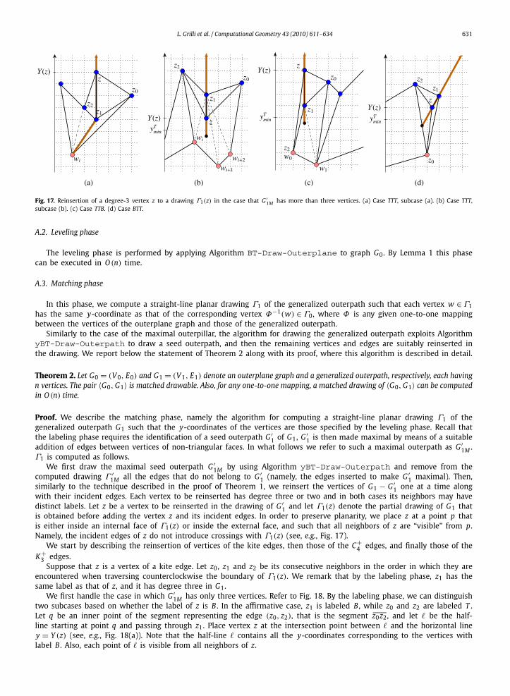
L. Grilli et al. / Computational Geometry 43 (2010) 611–634 631
Fig. 17. Reinsertion of a degree-3 vertex z to a drawing Γ1(z) in the case that G ′1M has more than three vertices. (a) Case TTT, subcase (a). (b) Case TTT,
subcase (b). (c) Case TTB. (d) Case BTT.
A.2. Leveling phase
The leveling phase is performed by applying Algorithm BT-Draw-Outerplane to graph G0. By Lemma 1 this phasecan be executed in O (n) time.
A.3. Matching phase
In this phase, we compute a straight-line planar drawing Γ1 of the generalized outerpath such that each vertex w ∈ Γ1has the same y-coordinate as that of the corresponding vertex Φ−1(w) ∈ Γ0, where Φ is any given one-to-one mappingbetween the vertices of the outerplane graph and those of the generalized outerpath.
Similarly to the case of the maximal outerpillar, the algorithm for drawing the generalized outerpath exploits AlgorithmyBT-Draw-Outerpath to draw a seed outerpath, and then the remaining vertices and edges are suitably reinserted inthe drawing. We report below the statement of Theorem 2 along with its proof, where this algorithm is described in detail.
Theorem 2. Let G0 = (V 0, E0) and G1 = (V 1, E1) denote an outerplane graph and a generalized outerpath, respectively, each havingn vertices. The pair 〈G0, G1〉 is matched drawable. Also, for any one-to-one mapping, a matched drawing of 〈G0, G1〉 can be computedin O (n) time.
Proof. We describe the matching phase, namely the algorithm for computing a straight-line planar drawing Γ1 of thegeneralized outerpath G1 such that the y-coordinates of the vertices are those specified by the leveling phase. Recall thatthe labeling phase requires the identification of a seed outerpath G ′
1 of G1, G ′1 is then made maximal by means of a suitable
addition of edges between vertices of non-triangular faces. In what follows we refer to such a maximal outerpath as G ′1M .
Γ1 is computed as follows.We first draw the maximal seed outerpath G ′
1M by using Algorithm yBT-Draw-Outerpath and remove from thecomputed drawing Γ ′
1M all the edges that do not belong to G ′1 (namely, the edges inserted to make G ′
1 maximal). Then,similarly to the technique described in the proof of Theorem 1, we reinsert the vertices of G1 − G ′
1 one at a time alongwith their incident edges. Each vertex to be reinserted has degree three or two and in both cases its neighbors may havedistinct labels. Let z be a vertex to be reinserted in the drawing of G ′
1 and let Γ1(z) denote the partial drawing of G1 thatis obtained before adding the vertex z and its incident edges. In order to preserve planarity, we place z at a point p thatis either inside an internal face of Γ1(z) or inside the external face, and such that all neighbors of z are “visible” from p.Namely, the incident edges of z do not introduce crossings with Γ1(z) (see, e.g., Fig. 17).
We start by describing the reinsertion of vertices of the kite edges, then those of the C+4 edges, and finally those of the
K +3 edges.
Suppose that z is a vertex of a kite edge. Let z0, z1 and z2 be its consecutive neighbors in the order in which they areencountered when traversing counterclockwise the boundary of Γ1(z). We remark that by the labeling phase, z1 has thesame label as that of z, and it has degree three in G1.
We first handle the case in which G ′1M has only three vertices. Refer to Fig. 18. By the labeling phase, we can distinguish
two subcases based on whether the label of z is B . In the affirmative case, z1 is labeled B , while z0 and z2 are labeled T .Let q be an inner point of the segment representing the edge (z0, z2), that is the segment z0z2, and let be the half-line starting at point q and passing through z1. Place vertex z at the intersection point between and the horizontal liney = Y (z) (see, e.g., Fig. 18(a)). Note that the half-line contains all the y-coordinates corresponding to the vertices withlabel B . Also, each point of is visible from all neighbors of z.

632 L. Grilli et al. / Computational Geometry 43 (2010) 611–634
Fig. 18. Reinsertion of a degree-3 vertex z to a drawing Γ1(z) in the case that G ′1M has three vertices. (a) Vertex z is labeled B . (b) Vertex z is labeled T
and vertex z2 is labeled B . (c) Vertex z is labeled T and vertex z0 is labeled B .
In the case that z and z1 are labeled T (see, e.g., Figs. 18(b) and 18(c)), exactly one end-vertex of the edge (z0, z2) islabeled B , thus segment z0z2 contains a point q having y-coordinate equal to yT
min − 1/2, where yTmin is the minimum
y-coordinate among those corresponding to the vertices with label T . Similarly to the previous case, we define as thehalf-line through z1 and starting at point q, we draw z at the intersection point between and the horizontal line y = Y (z).
Assume now that G ′1M has more than three vertices, hence the top and bottom paths are always defined. Refer to Fig. 17.
We remark that Γ1(z) contains a drawing Γ ′1 that, in turn, is obtained from Γ ′
1M by removing the edges that are added inorder to make G ′
1 maximal. We identify a suitable poly-line or half-line such that: (i) contains all the y-coordinatesof the vertices having the same label as the label of z; (ii) each point of is visible from all neighbors of z. Vertex z isplaced at the intersection point between and the horizontal line y = Y (z); recall that Y (z) has been computed during theleveling phase. More precisely, in order to draw vertex z we distinguish the following cases.
Case TTT. In this case, z and all its neighbors are labeled T . Recall that in a maximal outerpath two adjacent vertices of thetop path must be connected with the same vertex of the bottom path. Hence, by referring to the maximal outerpathG ′
1M , we can distinguish two subcases: (a) all neighbors of z are connected with the same vertex wi of the bottompath; (b) the neighbor z1 is adjacent to (at least) two distinct vertices of the bottom path.Figs. 17(a) and 17(b) show two examples of these subcases, where dashed segments represent edges of G ′
1M thatdo not belong to G ′
1. In the first subcase, is formed by the segment wi z1 and by the vertical half-line startingfrom z1 and going up. In the second subcase, is the vertical half-line through the vertex z1 and starting at point(X(z1), yT
min − 1/2).Case TTB. In this case, z0, z1 and z2 are labeled T , T , and B , respectively. Hence, vertex z2 is the first vertex of the bottom
path of G ′1M , which is also denoted as w0 or s; see, e.g., Fig. 17(c). Therefore, we can define as the vertical half-line
through the vertex z1 and starting at point (X(z1), yTmin − 1/2).
Case BTT. In this case, z0, z1 and z2 are labeled B , T , and T , respectively. They form the last face of the maximal outerpath.Namely, z1 is the last vertex of the top path of G ′
1M , which is also denoted as t or w1nb−1, where wnb−1 is the last
vertex of the bottom path and it coincides with z0. z2 is the vertex of the top path preceding z1, and is denotedas w0
nb−1. We then define as the half-line through the vertex z1, starting from the point of segment z0z2 having
y-coordinate equal to yTmin − 1/2; see, e.g., Fig. 17(d).
Case BBB. This case is symmetric to the case TTT.Case BBT. This case is symmetric to the case TTB.Case TBB. This case is symmetric to the case BTT.
The case in which z is a vertex of a C+4 edge can be handled similarly to the kite edge case, by defining as z0, z1 and z2
three consecutive vertices on the boundary of Γ1(z) such that z0 and z2 are the two neighbors of z. We remark that theremay be more than one vertex z attached to the same pair of neighbors z0 and z2, but the computed drawing stays planarbecause the inner vertex z1 is not adjacent to any removed vertex.
Finally, we consider the case in which z is a vertex of some K +3 edge. Let z0 and z1 denote the neighbors of z, such
that z1 is the first vertex encountered after z0 when traversing counterclockwise the boundary of Γ1(z). If both neighbors z0and z1 have the same label, then vertex z can be drawn as described in the proof of Theorem 1.
Otherwise, two cases are possible, namely z0 and z1 are labeled either T and B , or B and T , respectively. In the firstcase, z1 is the first vertex of the bottom path of G ′
1M and by the labeling phase, z has label T . Thus, we define as thevertical half-line starting at point q and going up, where q is the point of the segment z0z1 such that Y (q) = yT −1/2; see,
min
L. Grilli et al. / Computational Geometry 43 (2010) 611–634 633
Fig. 19. Reinsertion of a vertex z that belongs to some K +3 edge. (a) Vertices z0 and z1 are labeled T and B , respectively. (b) Vertices z0 and z1 are labeled
B and T , respectively.
e.g., Fig. 19(a). In the second case, z1 is the last vertex of the top path of G ′1M and z has label B . We define as the vertical
half-line starting at point q and going down, where q is the point of z0z1 such that Y (q) = yTmin − 1/2; see, e.g., Fig. 19(b).
Concerning the time complexity, observe that by Lemma 5 a BT-labeling of 〈G0, G1〉 can be obtained in O (n) time, forany given one-to-one mapping between V 0 and V 1. The leveling phase requires O (n) time, as shown in Lemma 1. In thematching phase, Algorithm yBT-Draw-Outerpath computes drawing Γ ′
1M in O (n) time, as shown in Lemma 2. Also, eachvertex of G1 − G ′
1 and its incident edges can be drawn in O (1) time, because only a constant number of algebraic operationsneed to be executed. Therefore, the overall time complexity for computing a matched drawing of the pair 〈outerplane,generalized outerpath〉, each having n vertices, is O (n) for any given one-to-one mapping between the vertices of theirvertex sets. �References
[1] U. Brandes, C. Erten, J. Fowler, F. Frati, M. Geyer, C. Gutwenger, S.-H. Hong, M. Kaufmann, S.G. Kobourov, G. Liotta, P. Mutzel, A. Symvonis, Coloredsimultaneous geometric embeddings, in: Proc. 13th Annual International Conference on Computing and Combinatorics (COCOON 2007), in: LectureNotes in Computer Science, vol. 4598, 2007, pp. 254–263.
[2] P. Brass, E. Cenek, C.A. Duncan, A. Efrat, C. Erten, D.P. Ismailescu, S.G. Kobourov, A. Lubiw, J.S.B. Mitchell, On simultaneous planar graph embeddings,Computational Geometry. Theory and Applications 36 (2) (2007) 117–130.
[3] S. Cabello, M. van Kreveld, G. Liotta, H. Meijer, B. Speckmann, K. Verbeek, Geometric simultaneous embeddings of a graph and a matching, in: Proc.17th Intern. Symp. on Graph Drawing (GD 2009), in: Lecture Notes in Computer Science, vol. 5849, 2009, pp. 183–194.
[4] J. Cappos, A. Estrella-Balderrama, J.J. Fowler, S.G. Kobourov, Simultaneous graph embedding with bends and circular arcs, Computational Geometry.Theory and Applications 42 (2) (2009) 173–182.
[5] C. Collins, S. Carpendale, Vislink: Revealing relationships amongst visualizations, IEEE Transactions on Visualization and Computer Graphics 13 (6)(2007) 1192–1199.
[6] G. Di Battista, P. Eades, R. Tamassia, I.G. Tollis, Graph Drawing, Prentice Hall, Upper Saddle River, NJ, 1999.[7] G. Di Battista, E. Nardelli, Hierarchies and planarity theory, IEEE Transactions on Systems, Man, and Cybernetics 18 (6) (1988) 1035–1046.[8] E. Di Giacomo, W. Didimo, G. Liotta, P. Palladino, Visual analysis of one-to-many matched drawings, in: Special issue on selected papers from the 16th
Intern. Symp. on Graph Drawing (GD 2008), Journal of Graph Algorithms and Applications 14 (1) (2010) 97–119.[9] E. Di Giacomo, W. Didimo, M. van Kreveld, G. Liotta, B. Speckmann, Matched drawings of planar graphs, in: Special issue on selected papers from the
15th Intern. Symp. on Graph Drawing (GD 2007), Journal of Graph Algorithms and Applications 13 (3) (2009) 423–445.[10] E. Di Giacomo, G. Liotta, Simultaneous embedding of outerplanar graphs, paths, and cycles, International Journal of Computational Geometry and
Applications 17 (2) (2007) 139–160.[11] C. Erten, S.G. Kobourov, Simultaneous embedding of planar graphs with few bends, Journal of Graph Algorithms and Applications 9 (3) (2005) 347–364.[12] A. Estrella-Balderrama, J.J. Fowler, S.G. Kobourov, Characterization of unlabeled level planar trees, Computational Geometry. Theory and Applica-
tions 42 (7) (2009) 704–721.[13] A. Estrella-Balderrama, E. Gassner, M. Jünger, M. Percan, M. Schaefer, M. Schulz, Simultaneous geometric graph embeddings, in: Proc. 15th Intern.
Symp. on Graph Drawing (GD 2007), in: Lecture Notes in Computer Science, vol. 4875, 2007, pp. 280–290.[14] J.J. Fowler, Unlabeled level planarity, Ph.D. thesis, University of Arizona, http://ulp.cs.arizona.edu/ulp-thesis.pdf, 2009.[15] J.J. Fowler, M. Jünger, S.G. Kobourov, M. Schulz, Characterizing simultaneous embedding with fixed edges, Electronic Notes in Discrete Mathematics 31
(2008) 41–44.[16] J.J. Fowler, S.G. Kobourov, Characterization of unlabeled level planar graphs, in: Proc. 15th Intern. Symp. on Graph Drawing (GD 2007), in: Lecture
Notes in Computer Science, vol. 4875, 2007, pp. 37–49.[17] F. Frati, Embedding graphs simultaneously with fixed edges, in: Proc. 14th Intern. Symp. on Graph Drawing (GD 2006), in: Lecture Notes in Computer
Science, vol. 4372, 2006, pp. 108–113.[18] F. Frati, M. Kaufmann, S. Kobourov, Constrained simultaneous and near simultaneous embeddings, Journal of Graph Algorithms and Applications 13 (3)
(2009) 447–465.[19] M. Geyer, M. Kaufmann, I. Vrt’o, Two trees which are self-intersecting when drawn simultaneously, Discrete Mathematics 309 (7) (2009) 1909–1916.[20] L. Grilli, S.-H. Hong, G. Liotta, H. Meijer, S.K. Wismath, Matched drawability of graph pairs and of graph triples, in: Proc. 3rd International Workshop
on Algorithms and Computation (WALCOM 2009), in: Lecture Notes in Computer Science, vol. 5431, 2009, pp. 322–333.[21] P. Healy, A. Kuusik, S. Leipert, A characterization of level planar graphs, Discrete Mathematics 280 (1–3) (2004) 51–63.

634 L. Grilli et al. / Computational Geometry 43 (2010) 611–634
[22] M. Jünger, S. Leipert, Level planar embedding in linear time, Journal of Graph Algorithms and Applications 6 (1) (2002) 67–113.[23] M. Jünger, S. Leipert, P. Mutzel, Level planarity testing in linear time, in: Proc. 6th Intern. Symp. on Graph Drawing (GD 1998), in: Lecture Notes in
Computer Science, vol. 1547, 1998, pp. 224–237.[24] M. Kaufmann, D. Wagner (Eds.), Drawing Graphs: Methods and Models, Springer-Verlag, 2001.[25] T. Nishizeki, Md.S. Rahman, Planar Graph Drawing, World Scientific, 2004.[26] K. Sugiyama, Graph Drawing and Applications for Software and Knowledge Engineers, World Scientific, 2002.