Exponential Random Graph Modeling for Complex Brain Networks

Exponential Random Graph Modeling for Complex BrainNetworksSean L. Simpson1*, Satoru Hayasaka1,2, Paul J. Laurienti2

1 Department of Biostatistical Sciences, Wake Forest University School of Medicine, Winston-Salem, North Carolina, United States of America, 2 Department of Radiology,

Wake Forest University School of Medicine, Winston-Salem, North Carolina, United States of America

Abstract

Exponential random graph models (ERGMs), also known as p* models, have been utilized extensively in the social scienceliterature to study complex networks and how their global structure depends on underlying structural components.However, the literature on their use in biological networks (especially brain networks) has remained sparse. Descriptivemodels based on a specific feature of the graph (clustering coefficient, degree distribution, etc.) have dominatedconnectivity research in neuroscience. Corresponding generative models have been developed to reproduce one of thesefeatures. However, the complexity inherent in whole-brain network data necessitates the development and use of tools thatallow the systematic exploration of several features simultaneously and how they interact to form the global networkarchitecture. ERGMs provide a statistically principled approach to the assessment of how a set of interacting local brainnetwork features gives rise to the global structure. We illustrate the utility of ERGMs for modeling, analyzing, and simulatingcomplex whole-brain networks with network data from normal subjects. We also provide a foundation for the selection ofimportant local features through the implementation and assessment of three selection approaches: a traditional p-valuebased backward selection approach, an information criterion approach (AIC), and a graphical goodness of fit (GOF)approach. The graphical GOF approach serves as the best method given the scientific interest in being able to capture andreproduce the structure of fitted brain networks.

Citation: Simpson SL, Hayasaka S, Laurienti PJ (2011) Exponential Random Graph Modeling for Complex Brain Networks. PLoS ONE 6(5): e20039. doi:10.1371/journal.pone.0020039

Editor: Olaf Sporns, Indiana University, United States of America

Received January 12, 2011; Accepted April 11, 2011; Published May 25, 2011

Copyright: � 2011 Simpson et al. This is an open-access article distributed under the terms of the Creative Commons Attribution License, which permitsunrestricted use, distribution, and reproduction in any medium, provided the original author and source are credited.

Funding: This work was supported by the Translational Science Institute of Wake Forest University (Translational Scholar Award, URL: http://www.wfubmc.edu/TSI.htm) and by the National Institute of Neurological Disorders and Stroke (NS070917, URL:http://www.ninds.nih.gov/). The funders had no role in study design,data collection and analysis, decision to publish, or preparation of the manuscript.

Competing Interests: The authors have declared that no competing interests exist.

* E-mail: [email protected]

Introduction

Brain networksWhole-brain connectivity analyses are gaining prominence in

the neuroscientific literature due to the need to understand how

various regions of the brain interact with one another. The

inherent complexity in the way these regions interact necessitates

studying the brain as a whole rather than just its individual parts.

The application of network and graph theory to the brain has

facilitated these whole-brain analyses and helped to uncover new

insights into the structure and function of the nervous system.

Structural and functional connectivity studies have revealed that

the brain exhibits the small-world properties [1–4]. These

properties are characterized by tight local clustering and efficient

long distance connections as described in the seminal work of [5].

Network models based on a given small-world property or other

local property (e.g., node degree (k)) have mostly been utilized as a

means to describe various brain networks. However, in order to

gain deeper insights into the complex neurobiological interactions

and changes that occur in many neurological conditions and

disorders, analysis methods that enable systematically assessing

several properties simultaneously are needed given the statistical

dependencies among these properties [6,7]. The exponential

random graph models discussed in this paper provide one such

analysis approach.

Exponential random graph modelsExponential random graph models (ERGMs), also known as p*

models [8–11], have been utilized extensively in the social science

literature to analyze complex network data as discussed in [12,13]

and others. However, the literature on their use in biological

networks (especially brain networks) has remained sparse.

Descriptive models based on a specific feature of the network

such as characteristic path length (L) and clustering coefficient (C)

have dominated connectivity research in neuroscience [14]. The

few inferential studies have employed relatively rudimentary

testing techniques such as the ANOVA used in [15] to examine

group differences based on one of these features. ERGMs provide

a statistically principled approach to the systematic exploration of

several features simultaneously and how they interact to form the

global network architecture. They allow parsimoniously modeling

the probability mass function (pmf) for a given class of graphs

based on a set of explanatory metrics (local features). The pmf can

then be used to determine the probability that any given graph is

drawn from the same distribution as the observed graph. These

models enable achieving an efficient representation of complex

network data structures and allow examining the way in which a

network’s global structure and function depend on its local

structure. That is, they provide a means of assessing how and to

what extent combinations of local (brain) structures produce global

network properties.

PLoS ONE | www.plosone.org 1 May 2011 | Volume 6 | Issue 5 | e20039

In ERGMs networks are analogous to a multivariate response

variable in regression analysis, with the explanatory metrics

quantifying local features of the network such as how clustered

connections are (short distance communication) or how well the

network transmits information globally (long distance communica-

tion). Fitted parameter values from the model can then be utilized to

understand particular emergent behaviors of the network (how local

features give rise to the global structure). These values can also be

used to simulate random realizations of networks that retain

constitutive characteristics of the original network.

A more intuitive way to view ERGMs in the brain network

context are as models that quantify the relative significance of

various graph/network measures (k, C, L, etc.), or their analogues,

in explaining the overall network structure, thus enabling generative

conjectures about global architecture. These models provide several

benefits for brain network researchers. They allow asking specific

questions about processes that may give rise to the network

architecture via the inclusion of explanatory metrics of choice.

ERGMs inherently account for any confounding bias, like the (N,

k)-dependence of network measures (where N is the number of

nodes and k the average degree) detailed in [6], when the potential

confounding variables are included in the model. The stochastic

nature of the model allows understanding and quantifying the

uncertainty (an intrinsic feature of complex biological processes)

associated with our observed brain network(s) [12]. Simulations

based on ERGM fits to brain networks (sets of selected network

measures and their parameter estimates) can provide insight into

biological variability via the distribution of possible brain networks

produced. However, currently, the computational intensiveness of

fitting ERGMs may preclude their use with very large networks

(e.g., voxel-based networks with tens of thousands of nodes) and

certain combinations of network measures.

Here we illustrate the utility of ERGMs for modeling, analyzing,

and simulating complex whole-brain network. We also provide a

foundation for the development of a ‘‘best assessment’’ ERGM for

analyzing complex brain networks. Appropriate statistical compar-

isons between networks (or groups of networks) via ERGMs

necessitates establishing one model (set of explanatory metrics/local

features) in order to extract comparable parameter estimates due to

the dependence of these features on each other. Toward this end,

we assess three potential methods of feature selection for ERGMs in

the brain network context. These approaches include a traditional

p-value based backward selection approach, an information

criterion approach (AIC), and a graphical goodness of fit (GOF)

approach. Although the latter two techniques have been discussed

in the context of ERGMS [16,17], no detailed comparisons have

been performed to determine whether the approaches generally

produce the same ‘‘best’’ model/set of features.

Materials and Methods

Ethics statementThis study included 10 volunteers representing a subset of a

previous study [18]. The study protocol, including all analyses

performed here, was approved by the Wake Forest University

School of Medicine Institutional Review Board. All subjects gave

written informed consent in accordance with the Declaration of

Helsinki.

Data and network constructionOur data include whole-brain functional connectivity networks

for 10 normal subjects aged 20–35 (5 female, average age 27.7

years old [4.7 SD]). Each network is comprised of 90 nodes

corresponding to the 90 brain regions (90 ROIs-Regions of

Interest) defined by the Automated Anatomical Labeling atlas

(AAL; [19]). The whole-brain networks were constructed based on

fMRI images using graph theory methods. For each subject, 120

images were acquired during 5 minutes of resting using a gradient

echo echoplanar imaging (EPI) protocol with TR/TE = 2500/

40 ms on a 1.5 T GE twin-speed LX scanner with a birdcage head

coil (GE Medical Systems, Milwaukee, WI). The acquired images

were motion corrected, spatially normalized to the MNI (Montreal

Neurological Institute) space and re-sliced to 4|4|5 mm voxel

size using an in-house processing script based on SPM99 package

(Wellcome Trust Centre for Neuroimaging, London, UK). The

resulting images were not smoothed in order to avoid artificially

introducing local spatial correlation [20].

The first step in performing the network construction was to

generate a whole brain connectivity matrix, or adjacency matrix

Aij

� �. This is a binary n|n matrix where n is the number of nodes

representing 90 ROIs. The matrix notes the presence or absence

of a connection between any two nodes (i and j). The

determination of a connection between i and j was done by

calculating a partial correlation coefficient adjusted for motion and

physiological noises (see [21] for further details).

An unweighted, undirected network was then generated for

each subject by applying a threshold to the correlation matrix to

yield an adjacency matrix Aij

� �. In order to compare data across

people, it is necessary to generate comparable networks. The

network was defined so that the relationship between the number

of nodes n and the average node degree K is the same across

different subjects. In particular, the network was defined so that

S = log(n)=log(K ) is the same across subjects, with S~2:8. This

relationship is based on the path length of a random network with

n nodes and average degree K [4,5], and can be re-written as

n~KS . Our analysis includes ERGM fits to these thresholded

whole-brain functional connectivity networks for each subject (an

example of which is shown in Figure 1).

Model definitionExponential random graph models have the following form

[22]:

Ph Y ~yð Þ~k hð Þ{1exp hTg yð Þ� �

: ð1Þ

Here Y is an n|n (n nodes) random symmetric adjacency matrix

representing a brain network from a particular class of networks,

with Yij~1 if an edge exists between nodes i and j and Yij~0

otherwise. Nodes represent locations in the brain (e.g., ROIs) and

edges represent functional or structural connections between

them. We statistically model the probability mass function (pmf)

Ph Y~yð Þð Þ of this class of networks as a function of the

prespecified network features defined by the p-dimensional vector

g yð Þ. This vector of explanatory metrics consists of covariates that

are functions of the network y and can contain any graph statistic

(e.g., number of paths of length two) or node statistic (e.g., brain

location of the node). The parameter vector hRp, associated with

g yð Þ, quantifies the relative significance of the network features in

explaining the structure of the network after accounting for the

contribution of all other network features in the model and must

be estimated. More specifically, h indicates the change in the

log odds of an edge existing for each unit increase in the

corresponding explanatory metric. If the h value corresponding to

a given metric is large and positive, then that metric plays a

considerable role in explaining the network architecture and is

more prevalent than in the null model (random network with the

probability of an edge existing (p)~0:5). Conversely, if the h value

ERG Modeling for Complex Brain Networks


is large and negative, then that metric still plays a considerable role

in explaining the network architecture but is less prevalent than in

the null model. Consequently, inferences can be made about

whether certain local features/substructures are observed in the

network more than would be expected by chance enabling

hypothesis development regarding the biological processes that

produce these structural properties. The normalizing constant

k qð Þ ensures that the probabilities sum to one. This approach

allows representing the global network structure by locally

specified explanatory metrics, thus providing a means to examine

the nature of networks that are likely to emerge from these effects.

The goal in defining g yð Þ is to identify local metrics that

concisely summarize the global (whole-brain) network structure.

Table 1 defines a subset of mathematically compatible explan-

atory network metrics (for further details see [16,23,24]). Several

analogs to these metrics for directed graphs have been detailed by

[25]. The GWD, GWESP, and GWDSP statistics discussed in [17]

help address degeneracy issues illuminated in [22] and [26]. These

issues concern the shape of the estimated pmf (e.g., a pmf in which

only a few graphs have nonzero probability) and can lead to lack of

model convergence and unreliable results. As noted by [16,27], the

most appropriate explanatory metrics vary by network type. Thus,

an exploration of which network metrics best characterize brain

networks has great appeal. Once the most appropriate statistics

have been established, parameter profiles hð Þ can be utilized to

classify and compare whole-brain networks. These parameter

profile comparisons require the use of a uniform set of explanatory

metrics for all networks (due to metric interdependencies) and

balanced networks (same number of nodes for all networks) due to

the dependence of the metrics on network size.

It is important to note that ERGMs can be thought of as a way

of parameterizing models for networks, and are not a ‘‘kind’’ of

network model in the way ‘‘model’’ is traditionally used in the

brain network literature. Most other network models, in theory,

should have an equivalent ERGM expression (though that specific

expression may not be convenient, parsimonious, etc.). For

instance, an ERGM with just the Edges metric (Table 1) in the

formulation i:e:,in g yð Þð Þ is equivalent to the Erdos-Renyi model.

Thus, ERGMs allow parameterizations that subsume most (if not

all) other network models.

Fitting of the ERGM in equation 1 is normally done with either

Markov chain Monte Carlo maximum likelihood estimation

(MCMC MLE) or maximum pseudo-likelihood estimation

(MPLE) ([28] contains details). Model fits with MPLE are much

simpler computationally than MCMC MLE fits and afford higher

convergence rates with large networks. However, properties of the

MPLE estimators are not well understood, and the estimates tend

to be less accurate than those of MCMC MLE. Here we employ

MCMC MLE to fit the model in equation 1 given that there were

no convergence issues. See [29] for further details about this

estimation approach which can be implemented in the statnet

package [23] for the R statistical computing environment.

Model selectionIn order to establish the most appropriate set of explanatory

metrics for each subject’s brain network and provide a foundation

for the development of a ‘‘best assessment’’ ERGM for analyzing

complex brain networks, we implemented and assessed three

model/metric selection methods. They include a traditional p-

value based backward selection approach [30], an information

criterion approach (AIC, [31]), and a graphical goodness of fit

(GOF) approach [17]. The latter two techniques are used most

often for metric selection in ERGMs [16,17]; and, to our

knowledge, no detailed comparisons have been performed to

determine whether the approaches generally produce the same

‘‘best’’ model. The p-value approach is based on removing metrics

that are not statistically significant. Whereas, the AIC approach

selects the set of metrics that produce the estimated distribution

most likely to have resulted in the observed data with a penalty for

additional metrics to ensure parsimony. Alternatively, the

graphical GOF method allows subjectively selecting the set of

explanatory metrics that produces the model most able to capture

and reproduce certain topological properties of the observed

network (see Appendix S1 for more details). For each approach

ERGMs were fitted to the 90-node unweighted, undirected brain

networks of the 10 subjects discussed previously. The potential

explanatory metrics g yð Þð Þ for each of the 10 networks are listed

by category in Table 2. The categories were chosen based on

properties of brain networks that are regarded as important in the

literature [14]. These metrics are analogous to typical brain

Figure 1. Network of subject 10 in brain space.doi:10.1371/journal.pone.0020039.g001



network metrics (e.g., clustering coefficient (C)) but have been

developed to be statistically compatible with ERGMs. Figure 2illustrates the calculation of the less widely used of these statistics,

namely GWESP, GWNSP, and GWDSP, on a six-node example

network. The distribution of the unweighted analogues of these

metrics (ESP, NSP, and DSP) is given for simplicity. The weighted

versions simply sum the values of the distribution giving less weight

to those with more shared partners. For this example we note that

the network has 1 set of connected nodes with 1 shared partners

(ESP0), 5 sets with 1 shared partner (ESP1), 1 set with 2 shared

partners (ESP2), and 0 sets with 3 or 4 shared partners (ESP3 and

ESP4). Further details on the metrics are provided in Table 1 and

[27]. The t parameters associated with GWESP, GWDSP,

GWNSP, and GWD were all assumed to be fixed and known

(for reasons outlined in [17]) and set to t~0:75 based on

preliminary analyses as this value generally led to better fitting

models according to all selection methods. The three aforemen-

tioned model selection approaches are outlined in Appendix S1.

Results

We implemented the model selection procedures delineated in

the previous section and Appendix S1 for each of the 10 subjects

using the statnet package [23] for the R statistical computing

environment. The resulting models (for each approach) and their

corresponding parameter estimates are displayed in Table 3.

These estimates quantify the relative significance of the given

metric in explaining the overall network structure; and, more

specifically, they specify how much the log odds of an edge existing

increases for each unit increase in the corresponding metric. For

example, the final graphical GOF model for subject 10 shows that

GWESP is the most important metric (other than the number of

edges) in describing the structure of the subject’s network given the

larger absolute value of the parameter estimate. Additionally, the

Table 1. Subset of explanatory network metrics.

Metric Description

Edges Number of edges in network

Two-Path Number of paths of length 2 in the network

k-Cycle Number of k-cycles in network

k-Degree Number of nodes with degree k

Geometrically weighted Weighted sum of the counts of each degree (i) weighted

degree (GWD) by the geometric sequence 1{exp {tf gð Þi , where

t is a decay parameter

Geometrically weighted Weighted sum of the number of connected nodes having exactly i

edge-wise shared partner (GWESP) shared partners weighted by the geometric sequence

1{exp {tf gð Þi , where t is a decay parameter

Geometrically weighted Weighted sum of the number of non-connected nodes having exactly i

non-edge-wise shared partner(GWNSP) shared partners weighted by the geometric sequence


Geometrically weighted Weighted sum of the number of dyadsa having exactly i

dyad-wise shared partner (GWDSP) shared partners weighted by the geometric sequence


Nodematch Number of edges (i,j) for which nodal attribute i

equals nodal attribute j

(e.g., brain location of node i~brain location of node j)

anode pair with or without edge.doi:10.1371/journal.pone.0020039.t001

Figure 2. Six-node example network. The edgewise, nonedgewise,and dyadwise shared partner distributions are (ESP0 , . . ., ESP4)~(1, 5, 1,0, 0), (NSP0 , . . ., NSP4)~(1, 4, 3, 0, 0), and (DSP0 , . . ., DSP4)~(2, 9, 4, 0, 0)respectively.doi:10.1371/journal.pone.0020039.g002

Table 2. Explanatory network metrics by category.

Category Metric(s)

1) Connectedness Edges, Two-Path

2) Local Clustering/Efficiency GWESP, GWDSP

3) Global Efficiency GWNSPa

4) Degree Distribution GWD

5) Location (in the brain) Nodematch

NOTE: See Table 1 for more details on the metrics.aNot inherently global, but helps produce models that accurately capture theglobal efficiency of our networks.

doi:10.1371/journal.pone.0020039.t002



positiveness of the estimate associated with GWESP indicates that

an edge that closes a triangle is more likely to exist than it would by

chance (i.e., the network has more clustering than a random

network where the probability of an edge is p~0:5) for the family

of networks represented by subject 10’s fitted model. As evidenced

by the results in Table 3, the three model selection methods can

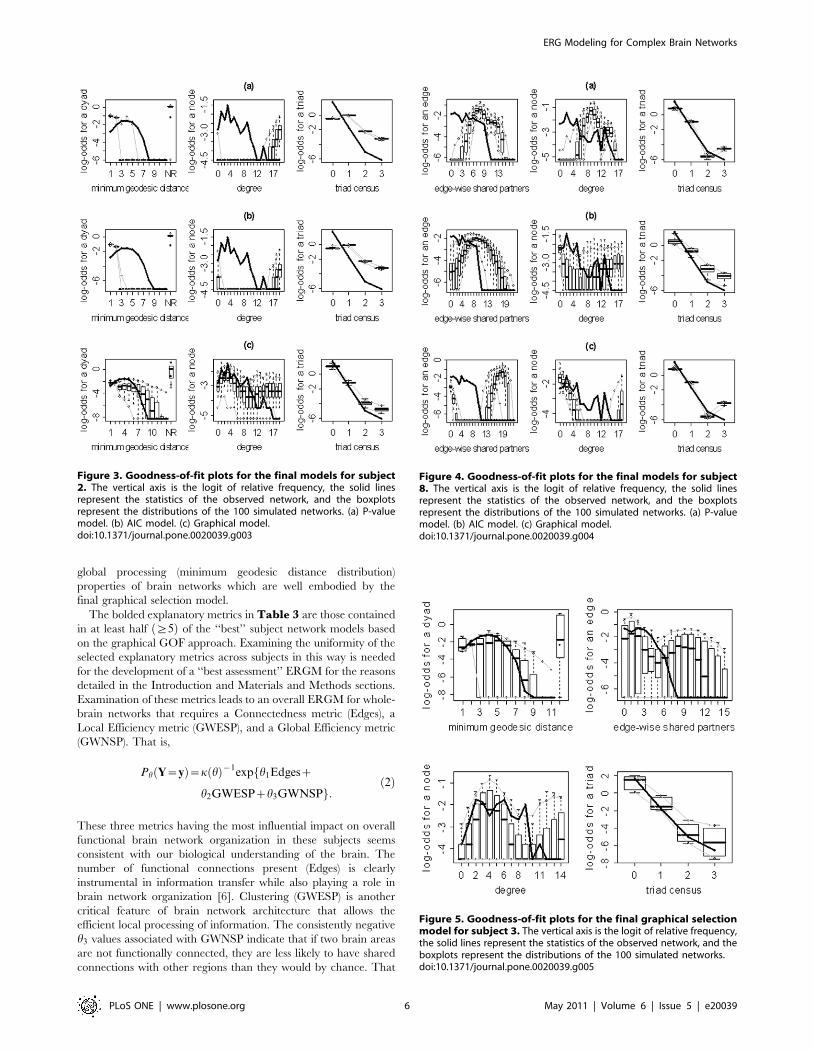
lead to very different ‘‘best’’ models. The disparate final model

GOF plots that can result from the three different model selection

approaches are exhibited in Figures 3 and 4 (for subjects 2 and

8). Again, our aim here is not to judge the three selection methods,

but to highlight the fact that they can lead to disparate final

models/sets of features. These model selection approaches have

been used seemingly arbitrarily in the literature; and, to our

knowledge, no detailed comparisons have been performed to

determine whether the approaches generally produce the same

‘‘best’’ model/set of features. For our purposes we recommend the

graphical GOF approach as the standard and will use it in future

analyses given that our main scientific interest lies in being able to

capture and reproduce the structure of the fitted brain networks.

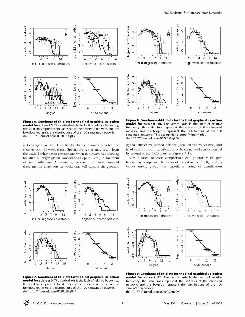
With the exception of subject 8, the graphical GOF approach

produces reasonably good fits for all subjects. The remaining best

graphical selection model GOF plots are shown in Figures 5–12.

Despite the obvious importance of Edges (as evidenced by the

absolute values of its parameter estimates in Table 3) in the

models, the overlap between the simulated and observed networks

in the GOF plots is not merely an effect of pure connectivity, but

also an effect of network organization. As mentioned in the

Materials and Methods section, an ERGM with just an Edges

metric is equivalent to the Erdos-Renyi random graph. Thus, due

to the small worldness of brain networks, models of this type will

not capture the tight local clustering/regional specificity (among

other properties) present in these networks [5]. Figure 13illustrates this point by exhibiting the disparate GOF plots for

an Edges only model and the final graphical selection model for

subject 10. Clearly the Edges only model is unable to capture the

regional specificity (edge-wise shared partners distribution) and

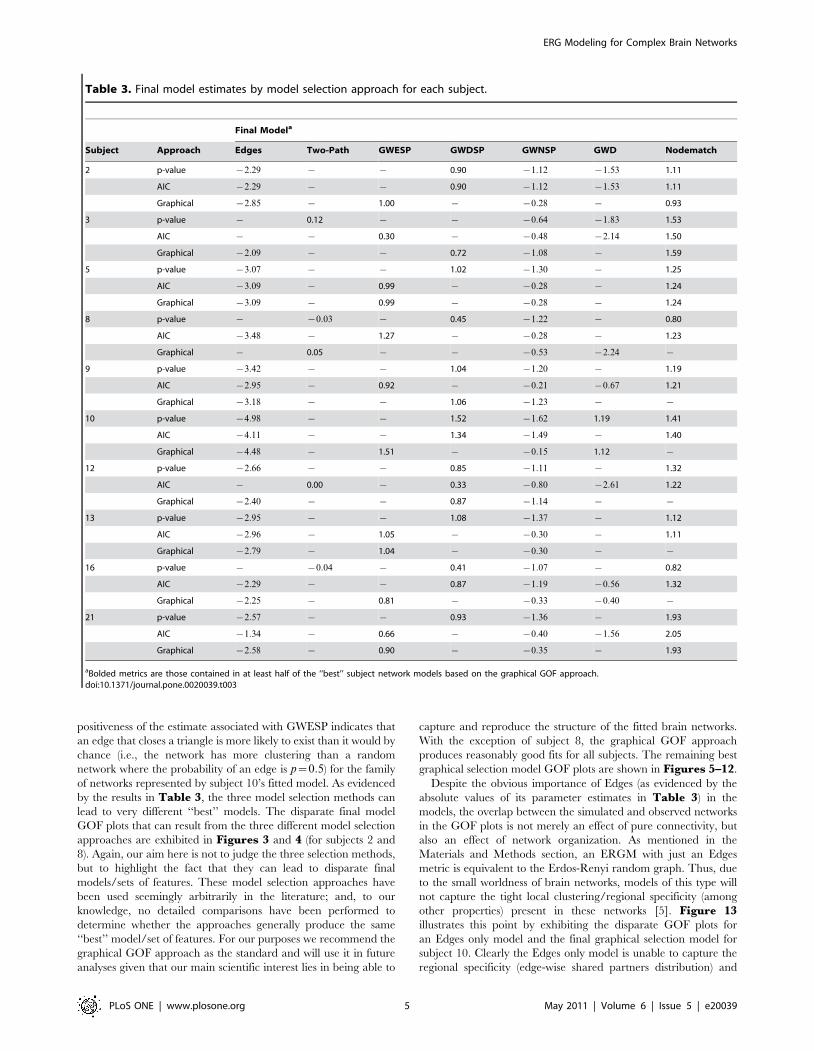
Table 3. Final model estimates by model selection approach for each subject.

Final Modela

Subject Approach Edges Two-Path GWESP GWDSP GWNSP GWD Nodematch

2 p-value {2:29 { { 0.90 {1:12 {1:53 1.11

AIC {2:29 { { 0.90 {1:12 {1:53 1.11

Graphical {2:85 { 1.00 { {0:28 { 0.93

3 p-value { 0.12 { { {0:64 {1:83 1.53

AIC { { 0.30 { {0:48 {2:14 1.50

Graphical {2:09 { { 0.72 {1:08 { 1.59

5 p-value {3:07 { { 1.02 {1:30 { 1.25

AIC {3:09 { 0.99 { {0:28 { 1.24

Graphical {3:09 { 0.99 { {0:28 { 1.24

8 p-value { {0:03 { 0.45 {1:22 { 0.80

AIC {3:48 { 1.27 { {0:28 { 1.23

Graphical { 0.05 { { {0:53 {2:24 {

9 p-value {3:42 { { 1.04 {1:20 { 1.19

AIC {2:95 { 0.92 { {0:21 {0:67 1.21

Graphical {3:18 { { 1.06 {1:23 { {

10 p-value {4:98 { { 1.52 {1:62 1.19 1.41

AIC {4:11 { { 1.34 {1:49 { 1.40

Graphical {4:48 { 1.51 { {0:15 1.12 {

12 p-value {2:66 { { 0.85 {1:11 { 1.32

AIC { 0.00 { 0.33 {0:80 {2:61 1.22

Graphical {2:40 { { 0.87 {1:14 { {

13 p-value {2:95 { { 1.08 {1:37 { 1.12

AIC {2:96 { 1.05 { {0:30 { 1.11

Graphical {2:79 { 1.04 { {0:30 { {

16 p-value { {0:04 { 0.41 {1:07 { 0.82

AIC {2:29 { { 0.87 {1:19 {0:56 1.32

Graphical {2:25 { 0.81 { {0:33 {0:40 {

21 p-value {2:57 { { 0.93 {1:36 { 1.93

AIC {1:34 { 0.66 { {0:40 {1:56 2.05

Graphical {2:58 { 0.90 { {0:35 { 1.93

aBolded metrics are those contained in at least half of the ‘‘best’’ subject network models based on the graphical GOF approach.doi:10.1371/journal.pone.0020039.t003



global processing (minimum geodesic distance distribution)

properties of brain networks which are well embodied by the

final graphical selection model.

The bolded explanatory metrics in Table 3 are those contained

in at least half §5ð Þ of the ‘‘best’’ subject network models based

on the graphical GOF approach. Examining the uniformity of the

selected explanatory metrics across subjects in this way is needed

for the development of a ‘‘best assessment’’ ERGM for the reasons

detailed in the Introduction and Materials and Methods sections.

Examination of these metrics leads to an overall ERGM for whole-

brain networks that requires a Connectedness metric (Edges), a

Local Efficiency metric (GWESP), and a Global Efficiency metric

(GWNSP). That is,

Ph Y~yð Þ~k hð Þ{1exp h1Edgeszf

h2GWESPzh3GWNSPg:ð2Þ

These three metrics having the most influential impact on overall

functional brain network organization in these subjects seems

consistent with our biological understanding of the brain. The

number of functional connections present (Edges) is clearly

instrumental in information transfer while also playing a role in

brain network organization [6]. Clustering (GWESP) is another

critical feature of brain network architecture that allows the

efficient local processing of information. The consistently negative

h3 values associated with GWNSP indicate that if two brain areas

are not functionally connected, they are less likely to have shared

connections with other regions than they would by chance. That

Figure 3. Goodness-of-fit plots for the final models for subject2. The vertical axis is the logit of relative frequency, the solid linesrepresent the statistics of the observed network, and the boxplotsrepresent the distributions of the 100 simulated networks. (a) P-valuemodel. (b) AIC model. (c) Graphical model.doi:10.1371/journal.pone.0020039.g003

Figure 4. Goodness-of-fit plots for the final models for subject8. The vertical axis is the logit of relative frequency, the solid linesrepresent the statistics of the observed network, and the boxplotsrepresent the distributions of the 100 simulated networks. (a) P-valuemodel. (b) AIC model. (c) Graphical model.doi:10.1371/journal.pone.0020039.g004

Figure 5. Goodness-of-fit plots for the final graphical selectionmodel for subject 3. The vertical axis is the logit of relative frequency,the solid lines represent the statistics of the observed network, and theboxplots represent the distributions of the 100 simulated networks.doi:10.1371/journal.pone.0020039.g005



is, two regions are less likely than by chance to have a 2-path as the

shortest path between them. Speculatively, this may result from

the brain having direct connections when necessary, but allowing

for slightly longer global connections (3-paths, etc.) to maintain

efficiency otherwise. Additionally, the synergistic combination of

these metrics engenders networks that well capture the geodesic

(global efficiency), shared partner (local efficiency), degree, and

triad census (motifs) distributions of brain networks as evidenced

by several of the GOF plots in Figures 3–13.

Group-based network comparisons can potentially be per-

formed by comparing the mean of the estimated h1, h2, and h3

values among groups via hypothesis testing or classification



Figure 8. Goodness-of-fit plots for the final graphical selectionmodel for subject 10. The vertical axis is the logit of relativefrequency, the solid lines represent the statistics of the observednetwork, and the boxplots represent the distributions of the 100simulated networks. This exemplifies a good fitting model.doi:10.1371/journal.pone.0020039.g008

Figure 9. Goodness-of-fit plots for the final graphical selectionmodel for subject 12. The vertical axis is the logit of relativefrequency, the solid lines represent the statistics of the observednetwork, and the boxplots represent the distributions of the 100simulated networks.doi:10.1371/journal.pone.0020039.g009



techniques. It is important to note that if one were to just compare

the mean of the estimated h1 (Edges) values among groups, for

instance, potential confounding from the GWESP and GWNSP

would be inherently accounted for given that the estimates account

for all other metrics in the model. In the hypothesis testing

Figure 10. Goodness-of-fit plots for the final graphicalselection model for subject 13. The vertical axis is the logit ofrelative frequency, the solid lines represent the statistics of theobserved network, and the boxplots represent the distributions ofthe 100 simulated networks.doi:10.1371/journal.pone.0020039.g010



Figure 13. Goodness-of-fit plots for the Edges only and finalgraphical selection models for subject 10. The vertical axis is thelogit of relative frequency, the solid lines represent the statistics of theobserved network, and the boxplots represent the distributions of the100 simulated networks. (a) Edges only model. (b) Final graphicalmodel.doi:10.1371/journal.pone.0020039.g013



framework one can exploit the fact that the h’s are approximate

MLEs and thus asymptotically have a Gaussian distribution.

Approximate T-tests and/or F-tests can then be employed.

Investigating the individual differences in final models among

subjects is also important. Although parameter values cannot be

directly compared when different models are fitted, the disparate

fits themselves may elucidate biologically interesting differences

among groups or individual subjects.

Here we implement our best assessment ERGM from equation

2 to illustrate its utility for comparing groups of networks. The

subjects were split into a younger (aged 20–26) and slightly older

(aged 29–35) group (5 subjects each) in order to assess if there were

any discernible differences between their brain networks. Other

studies have shown that older adults tend to have less clustering

and slightly more connections than their younger counterparts

[32,33]. However, direct comparisons have not been done on

groups of subjects this close in age to establish whether these

changes tend to commence immediately or take effect at older

ages. Moreover, these studies did not consider the potential

confounding effects of other network metrics when assessing these

differences. As evidenced by the results of our analysis exhibited in

Table 4, the two groups differ significantly in h3 (the GWNSP

parameter) with the younger group having a more negative value.

That is, if two nodes are not functionally connected, they are more

likely to have shared connections with other nodes in the brain

networks of the older group. Biologically, this could be the result of

the older brain maintaining two-path connections between brain

areas that have lost their direct connections; however, this

interpretation is purely speculative at this point. Interestingly,

there is not a statistically significant difference between the groups

for the Edges or GWESP parameter, with the trend being for the

older subjects’ networks to have more connections and clustering.

These findings run counter to those in the literature and may stem

from the fact that our analysis accounts for some of the

confounding that arises from network metric dependencies [6,7].

These disparate findings could also just be a result of the closeness

in age of the two groups or random variability given our small

sample size. As noted by [7], larger and methodologically more

comparable future investigations are needed to resolve many of the

contradictory findings in functional connectivity studies.

In addition to model representation and comparison, ERGMs

also provide a statistically sound method for simulating complex

brain networks as is done for the GOF plots. To illustrate their

utility in this context we simulated 100 networks based on the

fitted ERGM of subject 10. We then calculated several descriptive

metrics commonly used in the neuroimaging literature for the

observed and simulated networks to assess the utility of the

simulated networks within the neuroscientific context. Table 5displays the results of these computations for Clustering coefficient

(C), Characteristic path length (L), Local Efficiency (Eloc), Global

Efficiency (Eglob), and Mean Nodal Degree (K ) (see [4,34] for

details on these metrics). As evidenced by the results in this table,

the simulated networks are very similar to the observed network.

Hence ERGMs render an approach to simulating scientifically

meaningful brain networks.

Discussion

Our analyses in the previous section illustrate the utility of

ERGMs for modeling, analyzing, and simulating complex whole-

brain networks. We have also provided a foundation for the

development of a best assessment ERGM for the classification and

comparison of brain networks via the evaluation of three model/

feature selection approaches. The graphical GOF approach serves

as the best method given the scientific interest in being able to

capture and reproduce the structure of the fitted networks. The

greatest appeal of modeling brain networks with ERGMs lies in

their ability to efficiently represent this complex network data and

allow examining the way in which a network’s global structure and

function depend on local structural components.

There are a myriad of ways in which ERGMs can potentially be

useful for brain network researchers. As previously discussed and

demonstrated, groups of networks can be statistically compared

and classified (by disease status, age, task, etc.) based on several

network features simultaneously. The models also provide a way of

exploring which local features of brain networks are most

important in explaining their global architecture. As noted by

many authors [35–38], an analysis approach that can capture the

network characteristics from a group of subjects’ brain networks is

needed. ERGMs provide a potential solution since one could

average the parameter profiles, h, of a group and then simulate

‘‘representative’’ networks based on this averaged profile.

Preliminary work has shown this approach to be quite effective.

These representative networks can serve as null networks against

which other networks and network models can be compared, as

visualization tools, and as a means for characterizing properties of

network metrics in a group (e.g., community structure). ERGMs,

in general, will also serve to both accommodate the ever increasing

complexity of whole-brain analyses and inform future statistical

models for whole-brain research.

A computational limitation of note for brain network research-

ers is that MCMC MLE fits of ERGMs can be computationally

intensive and may fail to converge with more spatially resolved

networks than the 90 ROI ones used here. This fitting algorithm

has been shown to handle networks of several thousand nodes

[17]; however, its effectiveness is more dependent on the number

and topological structure of the edges than the node count [23].

Future work will examine the scalability of ERGMs fitted with

Table 4. Results of ERGM parameter estimate comparisonsbetween younger and older subjects.

Younger Older

Mean SE Mean SE P-value

h1 (Edges) {2:45 3.95|10{1 {3:09 3.47|10{1 0.2626

h2 (GWESP) 0.89 1.81|10{1 1.14 1.53|10{1 0.3339

h3 (GWNSP) {0:32 6.62|10{3 {0:24 4.79|10{3 v0:0001


Table 5. Network metrics of observed and simulatednetworks from subject 10.

Simulated Networks

MetricObservedValue Mean (SE)

Clustering coefficient (C) 0.447 0.468 (0.004)

Characteristic path length (L) 3.520 3.475 (0.033)

Local Efficiency (Eloc) 0.555 0.576 (0.004)

Global Efficiency (Eglob) 0.284 0.290 (0.003)

Mean Nodal Degree (K ) 5.066 4.939 (0.042)




MCMC MLE in the context of brain networks. As convergence

issues arise with more finely parcellated networks, MPLE fits may

serve as an appropriate alternative [16].

Another potential issue of note is that the original data’s

variability may affect the resulting ERGM fits. A given subject

may exhibit variability of the connections in their brain networks

at different times of day due to experimental or physiological

reasons. Assessment of the robustness of ERGM fits to this within-

subject variability is important and will be the focus of future

investigations.

In addition to the utility of ERGMs in the research context, the

potential implications of their use in the clinical context are

profound as they can aid in elucidating system level functional

features/neurological processes (represented by the explanatory

network metrics) that play a role in various cognitive disorders. For

instance, several authors have shown that schizophrenics have less

local efficiency in their brain networks [7,35,36] (which would

correspond to a smaller parameter estimate for GWESP in the

ERGM framework) than control subjects. ERGMs enable

empirically examining how this difference in efficiency affects

global brain structure and comparing these emergent whole-brain

brain networks between schizophrenics and controls. For example,

one could simulate networks based on model fits to schizophrenics

and controls to see how this difference affects the variability of the

resulting networks. This comparison may give us insight into the

neurological mechanisms that lead to schizophrenia (e.g., lack of

local neuronal communication leads to less stability in global

structure for schizophrenics).

Aside from the aforementioned clinical and biological work that

can be done with the models, there are also many possible

directions for future methodological research involving the analysis

of complex brain networks with ERGMs. Approximating the

small-sample distribution of h may prove useful for hypothesis

testing frameworks in which appealing to asymptotic normality

may not be appropriate. Developing methods for quantifying

GOF plots to remove subjectivity and allow for analytical

comparisons of the graph will be valuable. The approach should

allow some flexibility in determining how to weight the four

comparison statistics with respect to their relative importance to

the scientific context. Developing novel explanatory network

metrics rooted in both the biology of the brain and the

mathematics of ERGMs will engender better best assessment

models for network comparison. A corresponding hybrid model

selection approach where models are penalized for using many

covariates and the GOF plots are assessed will prove useful in

maintaining parsimony as the number of relevant explanatory

metrics increases. The extension of ERGMs to directed and/or

weighted brain networks will prove beneficial as construction of

these network types gains feasibility.

Supporting Information

Appendix S1 Model Selection

(PDF)

Acknowledgments

We thank the editor and referees for their comments that considerably

improved the paper. An earlier version of this manuscript can be found at

arxiv.org (Simpson et al., arXiv:1007.3230v1 [stat.AP]).

Author Contributions

Conceived and designed the experiments: SLS SH PJL. Performed the

experiments: SLS SH PJL. Analyzed the data: SLS SH PJL. Wrote the

paper: SLS SH PJL.

References

1. Iturria-Medina Y, Sotero RC, Canales-Rodriguez EJ, Aleman-Gomez Y, Melie-Garcia L (2008) Studying the human brain anatomical network via diffusion-

weighted MRI and graph theory. Neuro Image 40: 1064–1076.

2. Gong G, He Y, Concha L, Lebel C, Gross DW, et al. (2009) Mappinganatomical connectivity patterns of human cerebral cortex using in vivo diffusion

tensor imaging tractography. Cerebral Cortex 19: 524–536.

3. Bassett DS, Bullmore E (2006) Small-world brain networks. Neuroscientist 12:

512–523.

4. Stam CJ, Reijneveld JC (2007) Graph theoretical analysis of complex networks

in the brain. Nonlinear Biomedical Physics 1: 3.

5. Watts DJ, Strogatz SH (1998) Collective dynamics of small-world networks.

Nature 393: 440–442.

6. van Wijk BCM, Stam CJ, Daffertshofer A (2010) Comparing brain networks of

different size and connectivity density using graph theory. PLoS ONE 5(10): e13701.

7. Lynall ME, Bassett DS, Kerwin R, McKenna PJ, Kitzbichler M, et al. (2010)

Functional Connectivity and brain networks in schizophrenia. The Journal of

Neuroscience 30(28): 9477–9487.

8. Frank O, Strauss D (1986) Markov graphs. Journal of the American Statistical

Association 81: 832–842.

9. Pattison PE, Wasserman S (1999) Logit models and logistic regressions for socialnetworks: II. Multivariate relations. British Journal of Mathematical and

Statistical Psychology 52: 169–194.

10. Robins GL, Pattison PE, Wasserman S (1999) Logit models and logisticregression for social networks: III. Valued relations. Psychometrika 64: 371–394.

11. Wasserman S, Pattison PE (1996) Logit models and logistic regressions for social

networks: I. An introduction to Markov graphs and p*. Psychometrika 61: 401–425.

12. Robins GL, Pattison PE, Kalish Y, Lusher D (2007) An introduction to

exponential random graph (p*) models for social networks. Social Networks 29:

173–191.

13. Robins GL, Snijders T, Wang P, Handcock M, Pattison PE (2007) Recentdevelopments in exponential random graph (p*) models for social networks.

Social Networks 29: 192–215.

14. Bullmore E, Sporns O (2009) Complex brain networks: graph theoretical analysisof structural and functional systems. Nature Reviews Neuroscience 10: 186–198.

15. Meunier D, Achard S, Morcom A, Bullmore E (2009) Age-related changes in

modular organization of human brain functional networks. Neuro Image 44:715–723.

16. Saul ZM, Filkov V (2007) Exploring biological network structure using

exponential random graph models. Bioinformatics 23: 2604–2611.

17. Hunter DR, Goodreau SM, Handcock MS (2008) Goodness of fit of social

network models. Journal of the American Statistical Association 103: 248–258.

18. Peiffer AM, Hugenschmidt CE, Maldjian JA, Casanova R, Srikanth R, et al.

(2009) Aging and the interaction of sensory cortical function and structure.

Human Brain Mapping 30: 228–240.

19. Tzourio-Mazoyer N, Landeau B, Papathanassiou D, Crivello F, Etard O, et al.

(2002) Automated anatomical labeling of activations in SPM using a

macroscopic anatomical parcellation of the MNI MRI single-subject brain.

Neuro Image 15: 273–289.

20. van den Heuvel MP, Stam CJ, Boersma M, Hulshoff Pol HE (2008) Small-world

and scale free organization of voxel-based resting-state functional connectivity in

the human brain. Neuro Image 43: 528–539.

21. Hayasaka S, Laurienti PJ (2010) Comparison of characteristics between region- and

voxel based network analysis in resting-state fMRI. Neuro Image 50: 499–508.

22. Handcock MS (2002) Statistical models for social networks: Inference and

degeneracy. Dynamic Social Network Modelling and Analysis: Workshop

Summary and Papers. Breiger R, Carley K, Pattison PE, eds. Washington, DC:

National Academy Press. pp 229–240.

23. Handcock MS, Hunter DR, Butts CT, Goodreau SM, Morris M (2008) statnet:

Software tools for the statistical modeling of network data. URL http://

statnetproject.org.

24. Snijders TAB, Pattison PE, Robins GL, Handcock MS (2006) New specifications

for exponential random graph models. Sociological Methodology 36: 99–154.

25. Robins G, Pattison P, Wang P (2009) Closure, connectivity and degree

distributions: exponential random graph (p*) models for directed social networks.

Social Networks 31: 105–117.

26. Rinaldo A, Fienberg SE, Zhou Y (2009) On the geometry of discrete exponential

families with application to exponential random graph models. Electronic

Journal of Statistics 3: 446–484.

27. Morris M, Handcock MS, Hunter DR (2008) Specification of exponential-family

random raph models: terms and computational aspects. Journal of Statistical

Software 24.

28. van Duijn MAJ, Gile KJ, Handcock MS (2009) A framework for the comparison

of maximum pseudo-likelihood and maximum likelihood estimation of

exponential family random graph models. Social Networks 31: 52–62.



29. Hunter DR, Handcock MS, Butts CT, Goodreau SM, Morris M (2008) ergm: A

package to fit, simulate and diagnose exponential-family models for networks.

Journal of Statistical Software 24.

30. Muller KE, Fetterman BA (2002) Regression and ANOVA: an integrated

approach using SAS software. Cary, NC: SAS Institute Inc.

31. Akaike H (1974) A new look at the statistical model identification. IEEE

Transaction on Automatic Control AC-19: 716–723.

32. Gaal ZA, Boha R, Stam CJ, Molnar M (2009) Age-dependent features of EEG-

reactivity Spectral, complexity, and network characteristics. Neuroscience

Letters 479: 79–84.

33. Gong G, Rosa-Neto P, Carbonell F, Chen ZJ, He Y, Evans AC (2009) Age- and

gender related differences in the cortical anatomical network. Journal of

Neuroscience 29: 15684–15693.

34. Rubinov M, Sporns O (2010) Complex network measures of brain connectivity:

uses and interpretations. Neuroimage 52(3): 1059–1069.35. Rubinov M, Knock SA, Stam CJ, Micheloyannis S, Harris AWF, et al. (2007)

Small-world properties of nonlinear brain activity in schizophrenia. Human

Brain Mapping 30: 403–416.36. Alexander-Bloch AF, Gogtay N, Meunier D, Birn R, Clasen L, et al. (2010)

Disrupted modularity and local connectivity of brain functional networks inchildhood-onset schizophrenia. Frontiers in Systems Neuroscience 4: Article

147.

37. Meunier D, Lambiotte R, Fornito A, Ersche KD, Bullmore ET (2009)Hierarchical modularity in human brain functional networks. Frontiers in

Neuroinformatics 3: 37.38. Joyce KE, Laurienti PJ, Burdette JH, Hayasaka S (2010) A new measure of

centrality for brain networks. PLoS ONE 5(8): e12200.



Exponential Random Graph Modeling for Complex Brain Networks

Documents

Transcript of Exponential Random Graph Modeling for Complex Brain Networks