Adaptive Meshing for Finite Element Analysis of ...
27
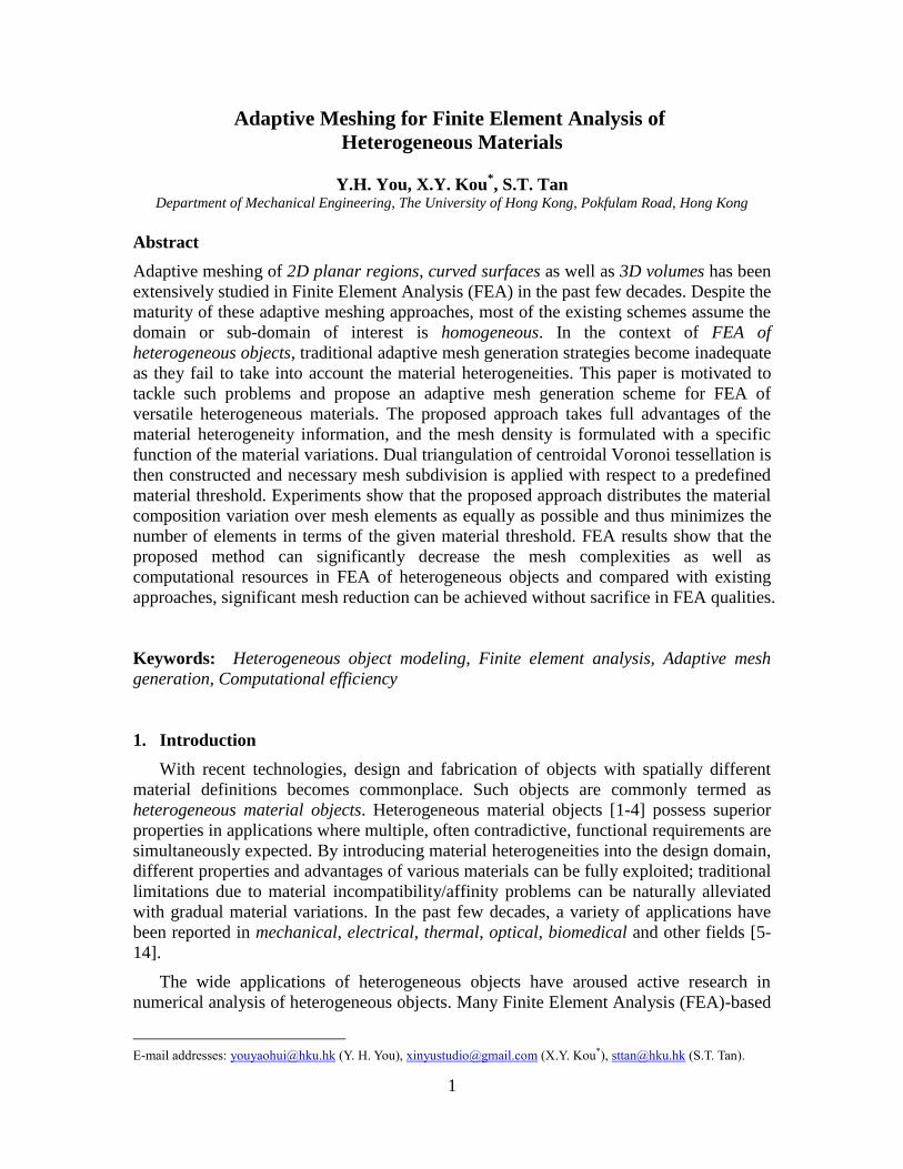
1 Adaptive Meshing for Finite Element Analysis of Heterogeneous Materials Y.H. You, X.Y. Kou * , S.T. Tan Department of Mechanical Engineering, The University of Hong Kong, Pokfulam Road, Hong Kong Abstract Adaptive meshing of 2D planar regions, curved surfaces as well as 3D volumes has been extensively studied in Finite Element Analysis (FEA) in the past few decades. Despite the maturity of these adaptive meshing approaches, most of the existing schemes assume the domain or sub-domain of interest is homogeneous. In the context of FEA of heterogeneous objects, traditional adaptive mesh generation strategies become inadequate as they fail to take into account the material heterogeneities. This paper is motivated to tackle such problems and propose an adaptive mesh generation scheme for FEA of versatile heterogeneous materials. The proposed approach takes full advantages of the material heterogeneity information, and the mesh density is formulated with a specific function of the material variations. Dual triangulation of centroidal Voronoi tessellation is then constructed and necessary mesh subdivision is applied with respect to a predefined material threshold. Experiments show that the proposed approach distributes the material composition variation over mesh elements as equally as possible and thus minimizes the number of elements in terms of the given material threshold. FEA results show that the proposed method can significantly decrease the mesh complexities as well as computational resources in FEA of heterogeneous objects and compared with existing approaches, significant mesh reduction can be achieved without sacrifice in FEA qualities. Keywords: Heterogeneous object modeling, Finite element analysis, Adaptive mesh generation, Computational efficiency 1. Introduction With recent technologies, design and fabrication of objects with spatially different material definitions becomes commonplace. Such objects are commonly termed as heterogeneous material objects. Heterogeneous material objects [1-4] possess superior properties in applications where multiple, often contradictive, functional requirements are simultaneously expected. By introducing material heterogeneities into the design domain, different properties and advantages of various materials can be fully exploited; traditional limitations due to material incompatibility/affinity problems can be naturally alleviated with gradual material variations. In the past few decades, a variety of applications have been reported in mechanical, electrical, thermal, optical, biomedical and other fields [5- 14]. The wide applications of heterogeneous objects have aroused active research in numerical analysis of heterogeneous objects. Many Finite Element Analysis (FEA)-based E-mail addresses: [email protected] (Y. H. You), [email protected] (X.Y. Kou * ), [email protected] (S.T. Tan).
-
Upload
khangminh22 -
Category
Documents
-
view
1 -
download
0
Transcript of Adaptive Meshing for Finite Element Analysis of ...
1
Adaptive Meshing for Finite Element Analysis of
Heterogeneous Materials
Y.H. You, X.Y. Kou*, S.T. Tan
Department of Mechanical Engineering, The University of Hong Kong, Pokfulam Road, Hong Kong
Abstract
Adaptive meshing of 2D planar regions, curved surfaces as well as 3D volumes has been
extensively studied in Finite Element Analysis (FEA) in the past few decades. Despite the
maturity of these adaptive meshing approaches, most of the existing schemes assume the
domain or sub-domain of interest is homogeneous. In the context of FEA of
heterogeneous objects, traditional adaptive mesh generation strategies become inadequate
as they fail to take into account the material heterogeneities. This paper is motivated to
tackle such problems and propose an adaptive mesh generation scheme for FEA of
versatile heterogeneous materials. The proposed approach takes full advantages of the
material heterogeneity information, and the mesh density is formulated with a specific
function of the material variations. Dual triangulation of centroidal Voronoi tessellation is
then constructed and necessary mesh subdivision is applied with respect to a predefined
material threshold. Experiments show that the proposed approach distributes the material
composition variation over mesh elements as equally as possible and thus minimizes the
number of elements in terms of the given material threshold. FEA results show that the
proposed method can significantly decrease the mesh complexities as well as
computational resources in FEA of heterogeneous objects and compared with existing
approaches, significant mesh reduction can be achieved without sacrifice in FEA qualities.
Keywords: Heterogeneous object modeling, Finite element analysis, Adaptive mesh
generation, Computational efficiency
1. Introduction
With recent technologies, design and fabrication of objects with spatially different
material definitions becomes commonplace. Such objects are commonly termed as
heterogeneous material objects. Heterogeneous material objects [1-4] possess superior
properties in applications where multiple, often contradictive, functional requirements are
simultaneously expected. By introducing material heterogeneities into the design domain,
different properties and advantages of various materials can be fully exploited; traditional
limitations due to material incompatibility/affinity problems can be naturally alleviated
with gradual material variations. In the past few decades, a variety of applications have
been reported in mechanical, electrical, thermal, optical, biomedical and other fields [5-
14].
The wide applications of heterogeneous objects have aroused active research in
numerical analysis of heterogeneous objects. Many Finite Element Analysis (FEA)-based
E-mail addresses: [email protected] (Y. H. You), [email protected] (X.Y. Kou*), [email protected] (S.T. Tan).
2
approaches have been proposed for function analysis or design validities [15-21]. These
methods extended traditional FEA approaches by taking the material heterogeneity into
account and allowing different materials to be defined for each node or element. Most of
them either use classic mesh generation schemes which result in poor accuracies (as the
mesh only guarantees the geometric accuracies but fails to characterize the material
heterogeneities) or alternatively, employ meshes with ultra-high densities to assure
solution accuracies, which, on the other hand, significantly degrades the computational
efficiencies [22].
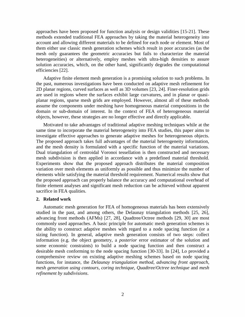
Adaptive finite element mesh generation is a promising solution to such problems. In
the past, numerous investigations have been conducted on adaptive mesh refinement for
2D planar regions, curved surfaces as well as 3D volumes [23, 24]. Finer-resolution grids
are used in regions where the surfaces exhibit large curvatures, and in planar or quasi-
planar regions, sparse mesh grids are employed. However, almost all of these methods
assume the components under meshing have homogeneous material compositions in the
domain or sub-domain of interest. In the context of FEA of heterogeneous material
objects, however, these strategies are no longer effective and directly applicable.
Motivated to take advantages of traditional adaptive meshing techniques while at the
same time to incorporate the material heterogeneity into FEA studies, this paper aims to
investigate effective approaches to generate adaptive meshes for heterogeneous objects.
The proposed approach takes full advantages of the material heterogeneity information,
and the mesh density is formulated with a specific function of the material variations.
Dual triangulation of centroidal Voronoi tessellation is then constructed and necessary
mesh subdivision is then applied in accordance with a predefined material threshold.
Experiments show that the proposed approach distributes the material composition
variation over mesh elements as uniformly as possible and thus minimize the number of
elements while satisfying the material threshold requirement. Numerical results show that
the proposed approach can properly balance the accuracy and computational overhead of
finite element analyses and significant mesh reduction can be achieved without apparent
sacrifice in FEA qualities.
2. Related work
Automatic mesh generation for FEA of homogeneous materials has been extensively
studied in the past, and among others, the Delaunay triangulation methods [25, 26],
advancing front methods (AFMs) [27, 28], Quadtree/Octree methods [29, 30] are most
commonly used approaches. A basic principle for automatic mesh generation schemes is
the ability to construct adaptive meshes with regard to a node spacing function (or a
sizing function). In general, adaptive mesh generation consists of two steps: collect
information (e.g. the object geometry, a posterior error estimator of the solution and
some economic constraints) to build a node spacing function and then construct a
desirable mesh conforming to the node spacing function [30-33]. In [24], Lo provided a
comprehensive review on existing adaptive meshing schemes based on node spacing
functions, for instance, the Delaunay triangulation method, advancing front approach,
mesh generation using contours, coring technique, Quadtree/Octree technique and mesh
refinement by subdivisions.
3
The aforementioned methods however mainly considered the geometric compatibility
and the topological compatibility of the finite element meshes. The geometric
compatibility guarantees the final mesh to be closely conformable to the object shapes or
geometries; and the topological compatibility ensures all the elements are properly
connected with correct adjacency relationships [34].
In addition to these two compatibility requirements, Sullivan et al. [34] proposed that
the physical compatibility should also be seriously considered, as he put it, “An accurate
numerical solution requires that the domain be discretized sufficiently to describe the
physics of the problem”. As such, they tackled the adaptive meshing problem for
heterogeneous objects, but unfortunately, they only focused on multi-material objects
which are very primitive in material heterogeneity. Schimpf et al. [35] also studied the
adaptive meshing problem for human organs (e.g. heart, liver, lungs), each of which is
also regarded as components with “distinct” materials.
The FEA studies on Functionally Graded Materials (FGMs) have been widely
investigated in recent years. Most investigations, however, did not take the local material
heterogeneities into account for the meshes were usually generated with commercial
software packages [36-39], which are inherently designed for homogeneous solid
modeling purposes.
To our knowledge, the work done by Shin [40], perhaps, seems to be the first study
on the adaptive meshing problem for FGM objects. In his work, he converted continuous
material gradation into step-wise variation. Iso-material contours of the solid model were
first created; triangular mesh was then generated inside each iso-material (i.e.
homogeneous) region formed by iso-material contours. The advantage of this model is
that it is computationally efficient, and the size of mesh elements is also adaptively
determined. However, only unidirectional material gradient was taken into account in
Shin’s approach. No generic solutions were proposed to solve adaptive mesh generation
for objects with bidirectional or even more complex material distributions [1, 41, 42].
Chiu et al. [43] proposed an adaptive mesh generation method for complex
heterogeneous objects based on the quadtree technique. A material threshold was utilized
to evaluate if a mesh element is homogenous or quasi-homogenous. The subdivision of
the domain was recursively processed until all the elements satisfied the material
threshold requirement. This method is capable of processing objects with complex
material gradient functions, for instance the Heterogeneous Feature Tree (HFT) structure
[42], but a large amount of computational resources are needed for geometric intersection
calculations. Moreover, material compositions are evaluated at a few sampling points
only (for instance, the corner points of a quadtree rectangle), and in case the material
composition differences among all sampling points fall below a given tolerance, no
further subdivisions will be performed any longer. Theoretically however, it is possible
that abrupt material changes still exist within quadrants of interest, even though the
material variations along the bounding edges are homogeneous or quasi-homogeneous. In
such scenarios, Chiu et al.’s approach is incapable of generating robust and adaptive
finite element meshes.
To the best of our knowledge, so far there seems to be no thorough investigations on
adaptive mesh generation for heterogeneous materials. Existing studies either resort to
4
commercial software packages, which by nature, are not suited for mesh generation of
heterogeneous materials, or use unnecessarily dense meshes which introduce significant
efficiency problems. This paper is motivated to bridge such a gap towards providing a
generic solution to this problem. We show, in what follows, that the proposed approach
can effectively generate adaptive meshes for general heterogeneous models, inclusive of
simple analytic function-based as well as other complex data representations such as HFT
structures.
3. Adaptive meshing of heterogeneous materials
In this section, a general scheme for adaptive meshing of heterogeneous materials is
first presented. Algorithmic details on how to apply the adaptive meshing method to
analytic function-based and HFT-based heterogeneous models are then elucidated with
examples.
3.1 General adaptive meshing scheme
For mesh generation of heterogeneous materials, there are four important factors to be
considered:
(i) Geometric approximation
In a numerical simulation by means of finite elements, the computational process is
based on an approximation (or mesh) of the domain where the problem is formulated. A
mesh that well conforms to the geometric boundaries is therefore a prerequisite for
accurate simulations.
(ii) Mesh quality
Mesh quality (e.g. aspect ratio) is another essential factor. Low-quality elements such
as skinny triangles with large aspect ratios will degrade the accuracy of FEA solutions or
lead to poor stiffness matrix conditioning [44].
(iii) Number of mesh elements
The number of mesh elements has significant impacts on the computational efficiency
of FEA. In order to boost the computational efficiency while maintaining the accuracy of
FEA solutions, it is crucial to avoid introducing an excessive number of mesh elements.
(iv) Material threshold
When heterogeneous materials are subjected to FEA, the material composition
variation, which directly relates to the material property (e.g. Young’s modulus) change
in each finite element, greatly impacts the accuracy of FEA solutions [45]. A material
threshold is proposed to evaluate the validity of meshes of heterogeneous materials. A
generated mesh T is deemed validated, when the maximum material composition
variation δmax over elements of T is lower than the material threshold δ0, i.e.
0Τ
, where max .max maxT
T
(1)
Here δ(T) denotes the material composition variation within an arbitrary element T in T .
To satisfy these four requirements, we propose an adaptive meshing scheme for
accurate and efficient FEA of heterogeneous materials, in which the mesh adaptivity is
determined by both material and geometric complexities of heterogeneous materials. In
light of that, the proposed adaptive meshing algorithm embraces three-step meshing
5
stages: Initial Mesh Generation (IMG), Material-Oriented Refinement (MOR) and
Geometry-Oriented Refinement (GOR).
The IMG only involves a classical mesh generation problem, in which an initial
triangulation that well approximates the geometric domain is constructed by a geometric
modeler. In this stage, no material heterogeneity information is taken into account.
Following the IMG step, the MOR is repeatedly executed until the generated mesh is
validated in terms of Eq. (1). In this mesh refinement step, a centroidal Voronoi
tessellation (CVT)-based approach is proposed to govern mesh adaptation. A density
function associated with material distributions being established, the CVT-based method
controls the mesh density in such a way that denser mesh nodes are accumulated into the
area where the material changing rate is large, and coarser nodes are allocated in relative
“flatter” regions, and here the flatness refers to the rate of material changes. In addition,
the CVT-based method distributes the material composition variation over elements of
the CVT-based mesh as uniformly as possible. In such a way, the number of elements is
minimized with respect to a predefined material threshold. The benefits of adopting the
CVT-based approach are two-fold: it enables easy and flexible controls on the mesh
distributions and also guarantees high mesh quality which is inherently supported due to
CVT's superior properties, as will be explained in more details in the following sections.
Notably, only material heterogeneity information is considered in the MOR. This
becomes problematic whenever coarse elements are generated near curved boundaries of
the domain where finer elements are expected to account for the geometric facilities. To
solve this problem, the third step of the adaptive meshing algorithm is applied. In the
GOR, the Delaunay refinement algorithm is used. Steiner points [25] are inserted into the
circumcenters of skinny triangles recursively until some specified criterion, such as
minimum angle, is satisfied.
As the Delaunay refinement algorithm applied in the GOR step has been well studied
[25, 26], our work in this paper focuses on the development of the MOR step, the core of
which is a CVT-based method. To make this paper self-contained, we first give a brief
introduction to the concept of CVT and its applications in the field of mesh generation.
3.1.1 Centroidal Voronoi tessellation
Given an open bounded domain d and a set of distinct points n
ii 1}{ x in Ω, the
corresponding Voronoi region Vi for each point xi is defined as:
for 1 and i i jV j ,...,n j i x x x x x (2)
where denotes the Euclidean distance in d . Note that the Voronoi region Vi is the
point set in Ω that are closer to xi than to any other point in n
ii 1}{ x . We refer to n
iiV 1}{ as
the Voronoi tessellation (VT) of Ω and n
ii 1}{ x as the associated generating points [46].
The dual tessellation of VT is called Voronoi Delaunay triangulation (VDT).
Given a nonnegative density function )(x on Ω, for any region V , the centroid
x* of V is defined as:
6
*
( )
.( )
V
V
d
d
x x x
xx x
(3)
We call a Voronoi tessellation n
iii V1
,
x of Ω a centroidal Voronoi tessellation
(CVT) if and only if the generating points n
ii 1}{ x corresponding to the Voronoi regions
n
iiV 1}{ are also the centroids of those regions, i.e., xi = xi* for i = 1, … , n [46]. The
associated Delaunay triangulation is called centroidal Voronoi Delaunay triangulation
(CVDT) [46].
A usually used algorithm for constructing CVT/CVDT is the Lloyd method [46].
Given a domain Ω, a density function x defined on Ω, and a positive integer n, the
Lloyd method is performed as below:
(i) Select an initial set of n points n
ii 1}{ x on Ω;
(ii) Construct the Voronoi regions n
iiV 1}{ of Ω associated with n
ii 1}{ x ;
(iii) Determine the mass centroids of the Voronoi regions n
iiV 1}{ ; these centroids form
the new set of points n
ii 1}{ x .
(iv) If the new points meet the convergence criteria, return n
iii V1
,
x and terminate;
otherwise, go to step (ii).
In recent years, extensive research efforts have been devoted to CVT/CVDT-based
mesh generation methods due to their superior properties in high-quality mesh generation
[47]. Du and Gunzburger [48] proposed a grid generation and optimization method based
on CVT/CVDT to create high-quality meshes over planes. Extensions of this method to
quality mesh generation of surfaces and solids were studied in [49, 50]. A brief overview
of the quality Delaunay triangulation methods based on CVT/CVDT can also be found in
[51]. When CVT/CVDT-based techniques are applied to construct high-quality meshes
over bounded domains, some generating points are required to lie on the domain
boundary so that the boundary conditions of FEA as well as the mesh quality can be
enforced [48]. In [48], various approaches that deal with the boundary generating points
are discussed, such as projecting the interior generating points to the boundary,
distributing a set of generating points on the boundary a priori, or a mixture of both
previous cases. Alternative to these methods, Ju [52] proposed the concept of conforming
CVT/CVDT (CfCVT/CfCVDT) in which a projection process as well as a special lifting
process is used to tackle the boundary generating points. A comprehensive study, which
compares various triangular mesh generators in terms of mesh quality, has shown that the
CfCVT/CfCVDT-based mesh generation method exhibits superiority in most cases [53].
Fig. 1 shows two CVT/CVDT-based meshes with respect to different density
functions. For a constant density function, the generating points n
ii 1}{ x are uniformly
distributed, which leads to high-quality mesh as shown in Fig. 1 (a). For a nonconstant
density function, the generating points n
ii 1}{ x are still locally uniformly distributed as
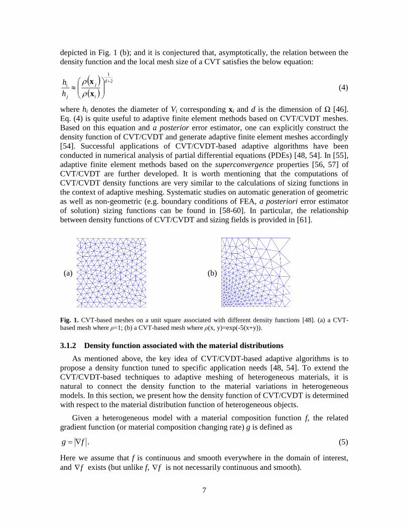
7
depicted in Fig. 1 (b); and it is conjectured that, asymptotically, the relation between the
density function and the local mesh size of a CVT satisfies the below equation:
2
1
d
i
j
j
i
h
h
x
x
(4)
where hi denotes the diameter of Vi corresponding xi and d is the dimension of Ω [46].
Eq. (4) is quite useful to adaptive finite element methods based on CVT/CVDT meshes.
Based on this equation and a posterior error estimator, one can explicitly construct the
density function of CVT/CVDT and generate adaptive finite element meshes accordingly
[54]. Successful applications of CVT/CVDT-based adaptive algorithms have been
conducted in numerical analysis of partial differential equations (PDEs) [48, 54]. In [55],
adaptive finite element methods based on the superconvergence properties [56, 57] of
CVT/CVDT are further developed. It is worth mentioning that the computations of
CVT/CVDT density functions are very similar to the calculations of sizing functions in
the context of adaptive meshing. Systematic studies on automatic generation of geometric
as well as non-geometric (e.g. boundary conditions of FEA, a posteriori error estimator
of solution) sizing functions can be found in [58-60]. In particular, the relationship
between density functions of CVT/CVDT and sizing fields is provided in [61].
(a)
(b)
Fig. 1. CVT-based meshes on a unit square associated with different density functions [48]. (a) a CVT-
based mesh where ρ=1; (b) a CVT-based mesh where ρ(x, y)=exp(-5(x+y)).
3.1.2 Density function associated with the material distributions
As mentioned above, the key idea of CVT/CVDT-based adaptive algorithms is to
propose a density function tuned to specific application needs [48, 54]. To extend the
CVT/CVDT-based techniques to adaptive meshing of heterogeneous materials, it is
natural to connect the density function to the material variations in heterogeneous
models. In this section, we present how the density function of CVT/CVDT is determined
with respect to the material distribution function of heterogeneous objects.
Given a heterogeneous model with a material composition function f, the related
gradient function (or material composition changing rate) g is defined as
.g f (5)
Here we assume that f is continuous and smooth everywhere in the domain of interest,
and f exists (but unlike f, f is not necessarily continuous and smooth).
8
In accordance with the gradient function, the desirable gradation of a CVT for the
heterogeneous model should follow the way that more generating points (or mesh nodes)
are created in the area where material composition changes quickly, while fewer
generating points are used in the area where material composition changes slowly. More
significantly, to minimize the number of generating points with regard to a material
threshold, the material composition variation over Voronoi regions of a CVT should be
distributed as equally as possible.
Let’s assume a CVT on a heterogeneous model satisfies the above equal material
variation property, thus we have
jjii hghg (6)
where gi denotes the mean value of g(x) on the Voronoi region Vi and hi denotes the
diameter of Vi. Note that when the number of Voronoi generating points gets large (or the
diameter of Voronoi regions becomes small), one can use the value of g(x) at the
generating point xi to approximate the mean value of g(x) on the Voronoi region Vi and
therefore
.i i j jg h g hx x (7)
From Eq. (4) and Eq. (7), it can be easily deduced that the relation between the
density function and the gradient function of material composition g follows the
below equation:
2 dcg (8)
where c is an arbitrary positive constant. For the sake of simplicity, we let c=1 and
rewrite the density function as
2.dg (9)
It turns out to be that the density function is a power function of the material
composition changing rate where d is the dimension of the domain of interest.
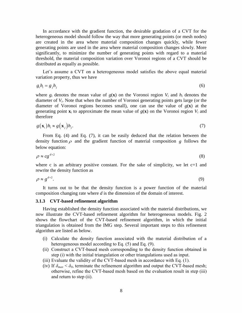
3.1.3 CVT-based refinement algorithm
Having established the density function associated with the material distributions, we
now illustrate the CVT-based refinement algorithm for heterogeneous models. Fig. 2
shows the flowchart of the CVT-based refinement algorithm, in which the initial
triangulation is obtained from the IMG step. Several important steps to this refinement
algorithm are listed as below.
(i) Calculate the density function associated with the material distribution of a
heterogeneous model according to Eq. (5) and Eq. (9).
(ii) Construct a CVT-based mesh corresponding to the density function obtained in
step (i) with the initial triangulation or other triangulations used as input.
(iii) Evaluate the validity of the CVT-based mesh in accordance with Eq. (1).
(iv) If δmax < δ0, terminate the refinement algorithm and output the CVT-based mesh;
otherwise, refine the CVT-based mesh based on the evaluation result in step (iii)
and return to step (ii).
9
Note that the CVT-based refinement algorithm involves an alternative process of
CVT-based mesh construction and mesh refinement. Here the CVT-based optimization
redistributes the positions of meshing points according to the density function to improve
mesh quality; the purpose of mesh refinement is to control the mesh size with respect to
the predefined material threshold. Compared to traditional refinement-based mesh
adaptation methods, the proposed algorithm generates adaptive meshes that conforms to
the sizing function with less node consumptions and guarantees good mesh qualities.
Similar algorithm was reported in [61], and various experiments have shown that CVT-
based refinement algorithms are superior to traditional ones [61].
Following the general scheme, we next take two heterogeneous models, namely the
analytic functional model (see Section 3.2) and the HFT-based model (see Section 3.3) as
examples to elucidate the rationale and general applicability of the adaptive meshing
method.
Fig. 2. Flowchart of the CVT-based refinement algorithm
3.2 Adaptive meshing for analytic functional model
Explicit, analytic functions are often used to represent heterogeneous material
distributions. Given a point ( , , )x y z in a Cartesian coordinate system, its material
composition is represented with an explicit analytic function ( , , )V f x y z . In the
literature, linear, exponential [21], parabolic [17] and power function [15] based material
distributions have been widely used in modeling heterogeneous objects. One common
property of all these functions is that their derivatives can be easily calculated. This
provides the basis for adaptive meshing of analytic functional models.
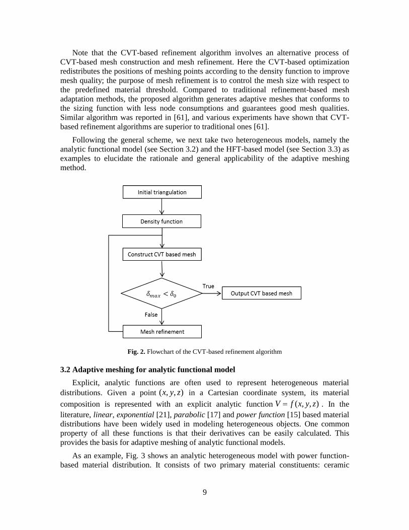
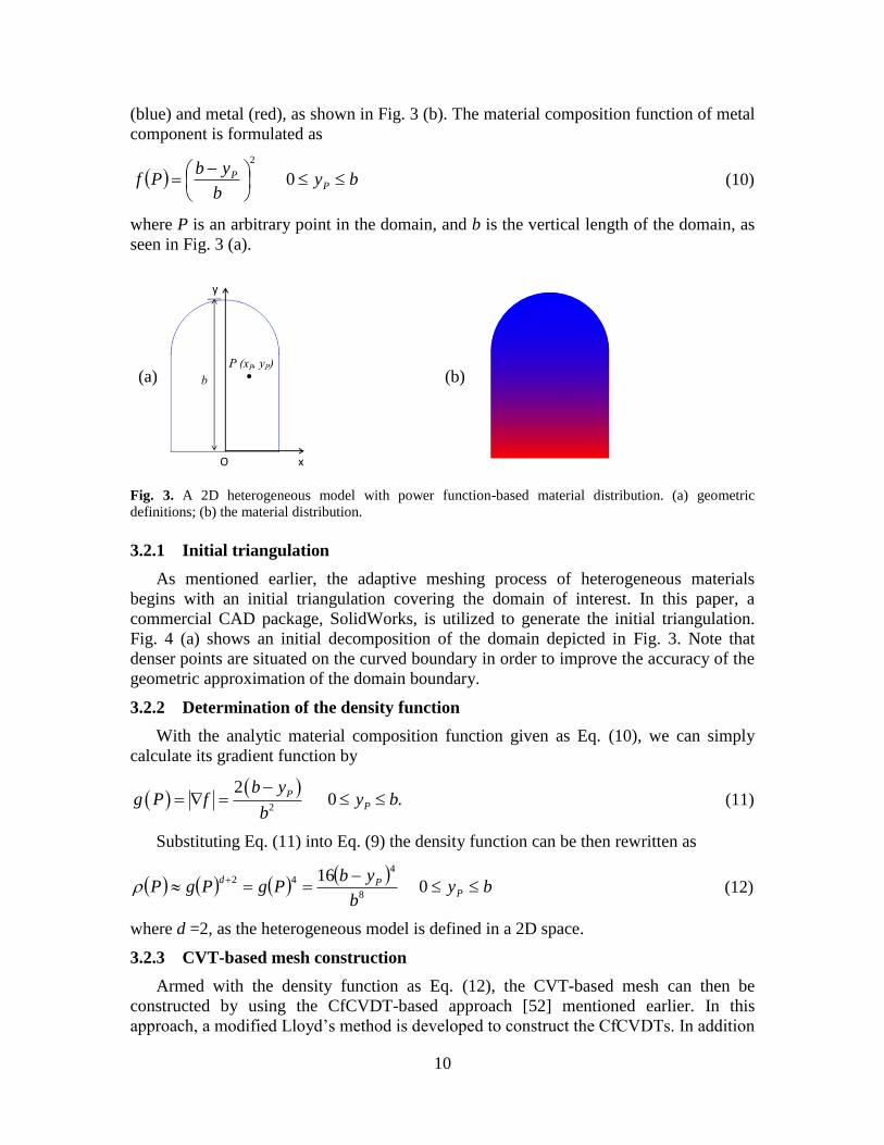
As an example, Fig. 3 shows an analytic heterogeneous model with power function-
based material distribution. It consists of two primary material constituents: ceramic
10
(blue) and metal (red), as shown in Fig. 3 (b). The material composition function of metal
component is formulated as
byb
ybPf P
P
0
2
(10)
where P is an arbitrary point in the domain, and b is the vertical length of the domain, as
seen in Fig. 3 (a).
(a)
(b)
Fig. 3. A 2D heterogeneous model with power function-based material distribution. (a) geometric
definitions; (b) the material distribution.
3.2.1 Initial triangulation
As mentioned earlier, the adaptive meshing process of heterogeneous materials
begins with an initial triangulation covering the domain of interest. In this paper, a
commercial CAD package, SolidWorks, is utilized to generate the initial triangulation.
Fig. 4 (a) shows an initial decomposition of the domain depicted in Fig. 3. Note that
denser points are situated on the curved boundary in order to improve the accuracy of the
geometric approximation of the domain boundary.
3.2.2 Determination of the density function
With the analytic material composition function given as Eq. (10), we can simply
calculate its gradient function by
2
2 0 .P
P
b yg P f y b
b
(11)
Substituting Eq. (11) into Eq. (9) the density function can be then rewritten as
byb
ybPgPgP P
Pd
0
168
442
(12)
where d =2, as the heterogeneous model is defined in a 2D space.
3.2.3 CVT-based mesh construction
Armed with the density function as Eq. (12), the CVT-based mesh can then be
constructed by using the CfCVDT-based approach [52] mentioned earlier. In this
approach, a modified Lloyd’s method is developed to construct the CfCVDTs. In addition
11
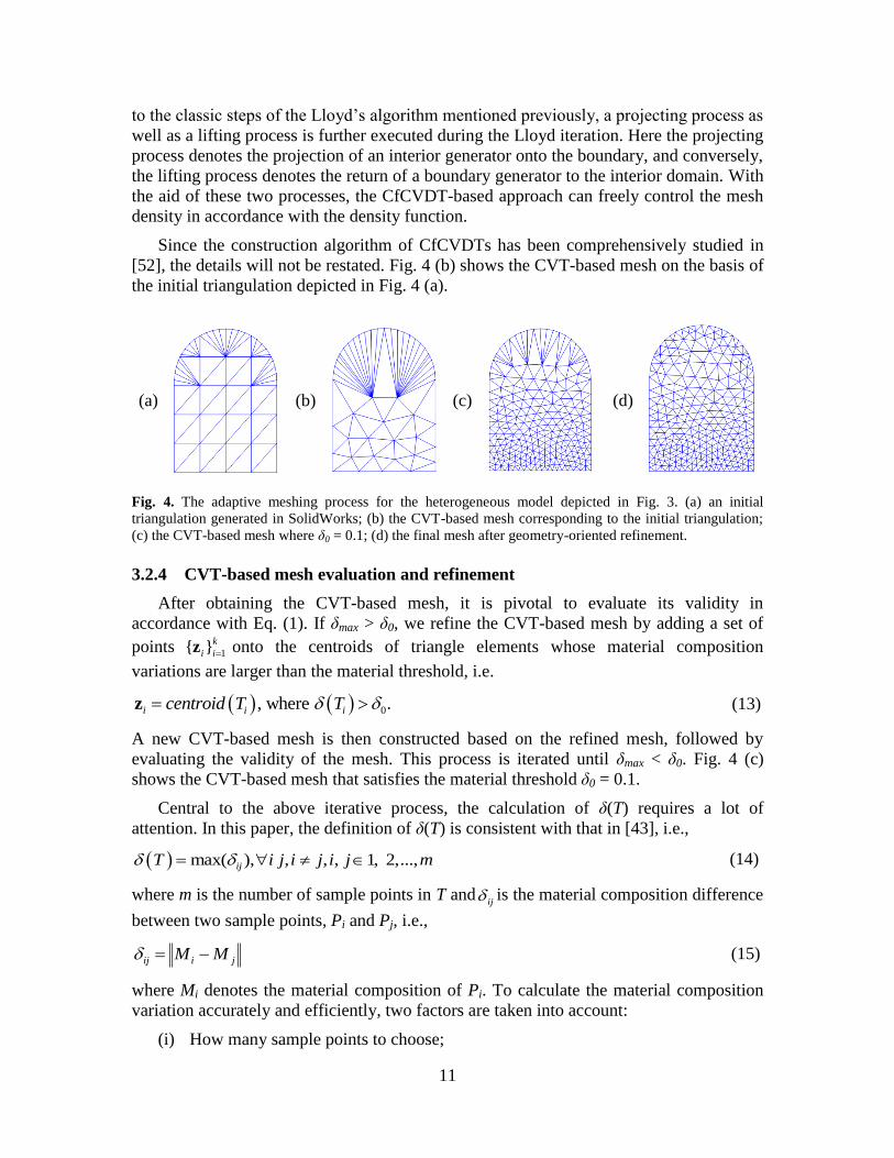
to the classic steps of the Lloyd’s algorithm mentioned previously, a projecting process as
well as a lifting process is further executed during the Lloyd iteration. Here the projecting
process denotes the projection of an interior generator onto the boundary, and conversely,
the lifting process denotes the return of a boundary generator to the interior domain. With
the aid of these two processes, the CfCVDT-based approach can freely control the mesh
density in accordance with the density function.
Since the construction algorithm of CfCVDTs has been comprehensively studied in
[52], the details will not be restated. Fig. 4 (b) shows the CVT-based mesh on the basis of
the initial triangulation depicted in Fig. 4 (a).
(a)
(b)
(c)
(d)
Fig. 4. The adaptive meshing process for the heterogeneous model depicted in Fig. 3. (a) an initial
triangulation generated in SolidWorks; (b) the CVT-based mesh corresponding to the initial triangulation;
(c) the CVT-based mesh where δ0 = 0.1; (d) the final mesh after geometry-oriented refinement.
3.2.4 CVT-based mesh evaluation and refinement
After obtaining the CVT-based mesh, it is pivotal to evaluate its validity in
accordance with Eq. (1). If δmax > δ0, we refine the CVT-based mesh by adding a set of
points k
ii 1}{ z onto the centroids of triangle elements whose material composition
variations are larger than the material threshold, i.e.
0, where .i i icentroid T T z (13)
A new CVT-based mesh is then constructed based on the refined mesh, followed by
evaluating the validity of the mesh. This process is iterated until δmax < δ0. Fig. 4 (c)
shows the CVT-based mesh that satisfies the material threshold δ0 = 0.1.
Central to the above iterative process, the calculation of δ(T) requires a lot of
attention. In this paper, the definition of δ(T) is consistent with that in [43], i.e.,
max( ), , , , 1, 2,...,ijT i j i j i j m
(14)
where m is the number of sample points in T andij is the material composition difference
between two sample points, Pi and Pj, i.e.,
jiij MM (15)
where Mi denotes the material composition of Pi. To calculate the material composition
variation accurately and efficiently, two factors are taken into account:
(i) How many sample points to choose;
12
(ii) Where to locate these points.
These being considered, one of the appropriate approaches is the adaptive sampling
process, in which more points are sampled in the region where material composition
changes rapidly while fewer points are sampled in the region where material composition
changes slowly. To satisfy such a sampling requirement, the nodes of CVT-based mesh
serve as sample points directly. In other words, the vertices of an element are used to
calculate the corresponding material composition variation and thus avoiding excessive
material interrogations at a large number of sampling points.
Similar to the definition of δmax in Eq. (1), we further define
Τ
T
1min , and
Tmin avg
TT
T TNum
(16)
where δmin and δavg denote the minimum and average material composition variation over
the elements of the mesh T , respectively.
3.2.5 Geometry-oriented refinement
In Fig. 4 (c), some skinny elements are induced near the curved boundary for the
value of the density function here is relatively low (see Eq. (12)) but dense vertices are
distributed on the curved boundary to precisely approximate the geometric features (refer
to Section 3.2.1). To further improve the mesh quality, we refine the mesh by using the
Ruppert’s refinement algorithm [25]. New points are inserted to the circumcenters of the
skinny triangles recursively until all triangles contain angles larger than a predefined
minimum angle.
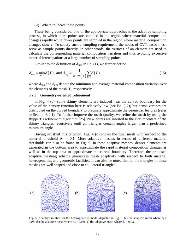
Having satisfied this criterion, Fig. 4 (d) shows the final mesh with respect to the
material threshold δ0 = 0.1. More adaptive meshes in terms of different material
thresholds can also be found in Fig. 5. In these adaptive meshes, denser elements are
generated in the bottom area to approximate the rapid material composition changes as
well as in the top area to approximate the curved boundary. Therefore the proposed
adaptive meshing scheme guarantees mesh adaptivity with respect to both material
heterogeneities and geometric facilities. It can also be noted that all the triangles in these
meshes are well shaped and close to equilateral triangles.
(a)
(b)
(c)
Fig. 5. Adaptive meshes for the heterogeneous model depicted in Fig. 3. (a) the adaptive mesh where δ0 =
0.08; (b) the adaptive mesh where δ0 = 0.05; (c) the adaptive mesh where δ0 = 0.03.
13
To evaluate the quality of a mesh, we apply a common quality measure [62], where
the quality of a triangle T is defined as
2 .T
T
b c a c a b a b cRq T
r abc
(17)
Here RT and Tr are the radii of the largest inscribed circle and the smallest circumscribed
circle of T, and a, b, c are the side lengths of T. Notice that equilateral triangles produce a
maximum q value of 1.0.
For a given triangulated mesh T , we further define
Τ Τ
T
1min , max , and
Tmin max avg
T TT
q q T q q T q q TNum
(18)
where qmin denotes the quality of the worst triangle, qmax denotes the quality of the best
triangle, and qavg denotes the average quality of the mesh T .
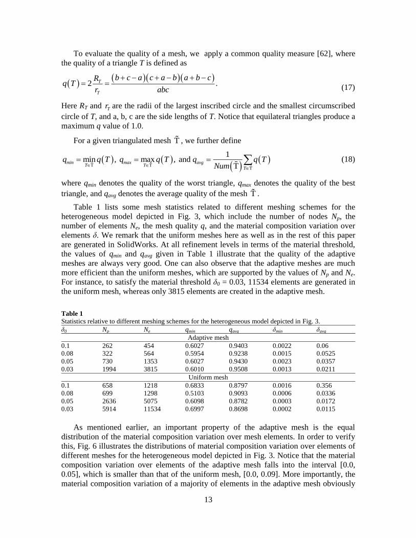
Table 1 lists some mesh statistics related to different meshing schemes for the
heterogeneous model depicted in Fig. 3, which include the number of nodes Np, the
number of elements Ne, the mesh quality q, and the material composition variation over
elements δ. We remark that the uniform meshes here as well as in the rest of this paper
are generated in SolidWorks. At all refinement levels in terms of the material threshold,
the values of qmin and qavg given in Table 1 illustrate that the quality of the adaptive
meshes are always very good. One can also observe that the adaptive meshes are much
more efficient than the uniform meshes, which are supported by the values of Np and Ne.
For instance, to satisfy the material threshold δ0 = 0.03, 11534 elements are generated in
the uniform mesh, whereas only 3815 elements are created in the adaptive mesh.
As mentioned earlier, an important property of the adaptive mesh is the equal
distribution of the material composition variation over mesh elements. In order to verify
this, Fig. 6 illustrates the distributions of material composition variation over elements of
different meshes for the heterogeneous model depicted in Fig. 3. Notice that the material
composition variation over elements of the adaptive mesh falls into the interval [0.0,
0.05], which is smaller than that of the uniform mesh, [0.0, 0.09]. More importantly, the
material composition variation of a majority of elements in the adaptive mesh obviously
Table 1 Statistics relative to different meshing schemes for the heterogeneous model depicted in Fig. 3.
δ0 Np Ne qmin qavg δmin δavg
Adaptive mesh
0.1 262 454 0.6027 0.9403 0.0022 0.06
0.08 322 564 0.5954 0.9238 0.0015 0.0525
0.05 730 1353 0.6027 0.9430 0.0023 0.0357
0.03 1994 3815 0.6010 0.9508 0.0013 0.0211
Uniform mesh
0.1 658 1218 0.6833 0.8797 0.0016 0.356
0.08 699 1298 0.5103 0.9093 0.0006 0.0336
0.05 2636 5075 0.6098 0.8782 0.0003 0.0172
0.03 5914 11534 0.6997 0.8698 0.0002 0.0115

14
concentrates to the interval [0.03, 0.04], which cannot be found in the uniform mesh. In
addition, from Table 1, one can also note that the average material composition of the
adaptive mesh (e.g. 0.0357) is much closer to the material threshold (e.g. 0.05) than that
of the uniform mesh (e.g. 0.0172). In light of the above observations, the adaptive
meshing scheme indeed distributes the material composition variation more equally than
does the uniform meshing sheme.
(a)
(b)
Fig. 6. Distributions of material composition variation over different meshes for the heterogeneous model
depicted in Fig. 3. (a) the distribution material composition variation over the adaptive mesh with 1353
elements; (b) the distribution of material composition variation over the uniform mesh with 1368 elements.
3.3 Adaptive meshing for complex hierarchical model
In the above function-based heterogeneous model, it is assumed that the function is
continuous and the derivative of the function exists. In practical applications, such a
constraint is often too restrictive, and the representable material heterogeneity is therefore
limited and simple. Complex (e.g. bidirectional or even tri-variate) heterogeneous
material distributions have proven to perform better in certain applications, especially
when the objects of interest have complex, irregular shapes or are subject to unbalanced
loads [20, 63]. In these scenarios, it is challenging to represent complex material
gradations with a single, analytic function throughout the entire geometric domain.
(a)
(b)
(c)
Fig. 7. A 2D heterogeneous object based on HFT structure. (a) material distribution; (b) the HFT structure;
(c) child features of the HFT structure.
In our previous work [41, 42], we proposed to use dedicated tree data structures to
represent heterogeneities that can hardly be represented with explicitly analytic functions.

15
A HFT structure was proposed to organize the material variation dependencies [42, 64]
with one or more hierarchies. By definition, heterogeneous features (saved in a tree node)
in the lower hierarchy represent the references from/to which the volume fractions vary,
and the parent feature represents the heterogeneous objects. As an example, Fig. 7 shows
a 2D heterogeneous object based on the HFT structure.
In this example, the 2D region F2D’s material gradation is dependent on the boundary
(Fb) and interface (Fint) curves; therefore, these curve features are saved as the child
features of the region F2D (see Fig. 7 (b)). For the boundary feature (Fb), its material
compositions are case specific, depending on the different location of the point of
interest, as shown in Fig. 7 (c). If the point is located between Circle A (CA) and Circle C
(CC), the material composition of CC represents the material composition of the boundary
feature; if the point is situated between CA and Circle B (CB), then CB represent the
material composition of the boundary feature instead of CC. Therefore, CB and CC are
saved as the child features of Fb (see Fig. 7 (b)).
As is evident above, no analytic function is used to represent the heterogeneous
material distribution, and the gradient function for the entire modeling domain is
unknown or even does not exist. Therefore the approach presented in Section 3.2 cannot
be directly migrated to the HFT-based model. Inspired by the hierarchical nature of the
HFT structure, we propose a divide and conquer-based approach to tackle the adaptive
meshing problem for the HFT-based model. The main steps of the proposed approach are
listed as below:
(i) Subdivide the domain of a HFT-based model into subregions that each subregion
has one unique material distribution;
(ii) Calculate the density function in each subregion;
(iii) Combine all the density functions of subregions into a density function over the
whole domain;
(iv) Generate an adaptive mesh of the HFT-based model with respect to the density
function obtained in step (iii).
In what follows, details about this approach are presented step by step.
3.3.1 Subdivision of the domain
According to the HFT-based model depicted in Fig. 7, for an arbitrary point Pi inside
the domain, the constituent composition of one primary material at this point is defined
as:
, 1 ,i bi inti int bi inti bf P W d d M W d d M (19)
where W is a user defined weighting function, dinti/dbi are the distances from Pi to the
interface/boundary features, and Mint/Mb are the material compositions (in terms of one
primary material) of the interface/boundary features.
As the material composition of the boundary feature (Mb) depends on its two child
features (CB and CC), we split the domain into two subregions (Ω1 and Ω2), each of which
has one unique material distribution, as shown in Fig. 7 (c). Without loss of generality,
the weighting function W is defined separately on each subregion as

16
2
1 1
3
2 2
, for ;
, for .
bibi inti i
inti bi
bibi inti i
inti bi
dW d d P
d d
dW d d P
d d
(20)
3.3.2 Calculation of the density functions in subregions
In the subregion Ω1, the material composition of an arbitrary point Pi can be written
as
B
AB
biBAi M
d
dMMPf
2
)( (21)
where MA and MB denotes the material composition of CA and CB, and dAB denotes the
distance between CA and CB, as shown in Fig. 7 (c). Accordingly, the derivative of this
material composition function can be calculated as:
2
2( ) ( ) .A B bi
i i
AB
M M dg P f P
d
(22)
Substituting Eq. (22) and Eq. (9) into with d = 2 yields
4 4
4
8
16( ) .A B bi
i i
AB
M M dP g P
d
(23)
Using the same approach, it is easy to know that for an arbitrary point Pi in Ω2, the
density function can be written as
4 4
12
81.A C bi
i
AC
M M dP
d
(24)
3.3.3 Combination of the density functions of subregions
Since the density function does not have to be continuous over the whole domain as
mentioned earlier, we simply combine the density functions of subregions into a
complete density function by
4 4
18
4 4
212
16
.81
A B bi
i
AB
i
A C bi
i
AC
M M dP
dP
M M dP
d
(25)
Table 2
Coefficients for the density function in Eq. (25)
MA MB MC dAC dAB
0.4 0 1 10 mm 20 mm

17
Table 2 lists the coefficients of this density function, upon which the following
adaptive meshing procedure depends.
3.3.4 Adaptive mesh generation with respect to the density function
Following the same approach as presented in Section 3.2, the adaptive mesh for the
complex HFT-based heterogeneous model can be generated. Fig. 8 shows two adaptive
meshes with respect to different material thresholds for the heterogeneous model depicted
in Fig. 7. Note that denser elements are accumulated to the interface curve (the red curve)
to approximate the rapid material composition changes as well as in the boundary areas to
approximate the curved boundaries. Therefore the proposed adaptive meshing scheme
guarantees mesh adaptivity with respect to both material heterogeneities and geometric
facilities.
(a)
(b)
Fig. 8. Adaptive meshes for the heterogeneous model depicted in Fig. 7. (a) the adaptive mesh where δ0 =
0.15; (b) the adaptive mesh where δ0 = 0.1.
Table 3 Statistics relative to the different meshing schemes for the heterogeneous model depicted in Fig. 7.
δ Np Ne qmin qavg δmin δavg
Adaptive mesh
0.15 1010 1820 0.5777 0.9161 0.0000 0.0625
0.10 1450 2700 0.5356 0.9247 0.0000 0.0556
0.08 2199 4198 0.5224 0.9302 0.0000 0.0443
0.05 4621 9042 0.5657 0.9382 0.0000 0.0346
Uniform mesh
0.15 1734 3319 0.6525 0.9625 0.0001 0.0445
0.10 4142 8024 0.5356 0.9247 0.0000 0.0287
0.08 6517 12707 0.5250 0.9598 0.0000 0.0228
0.05 17383 34231 0.4919 0.9544 0.0000 0.0141
Table 3 lists some mesh statistics relative to different meshing schemes for the
heterogeneous model depicted in Fig. 7. The values of qmin and qavg given in Table 3
18
demonstrate that the quality of the adaptive meshes is always very good at all refinement
levels in terms of the material threshold. One can also observe that the adaptive meshes
are much more efficient than the uniform meshes. For instance, to satisfy the material
threshold δ0 = 0.05, 34231 elements are generated in the uniform mesh, whereas only
9042 elements are created in the adaptive mesh.
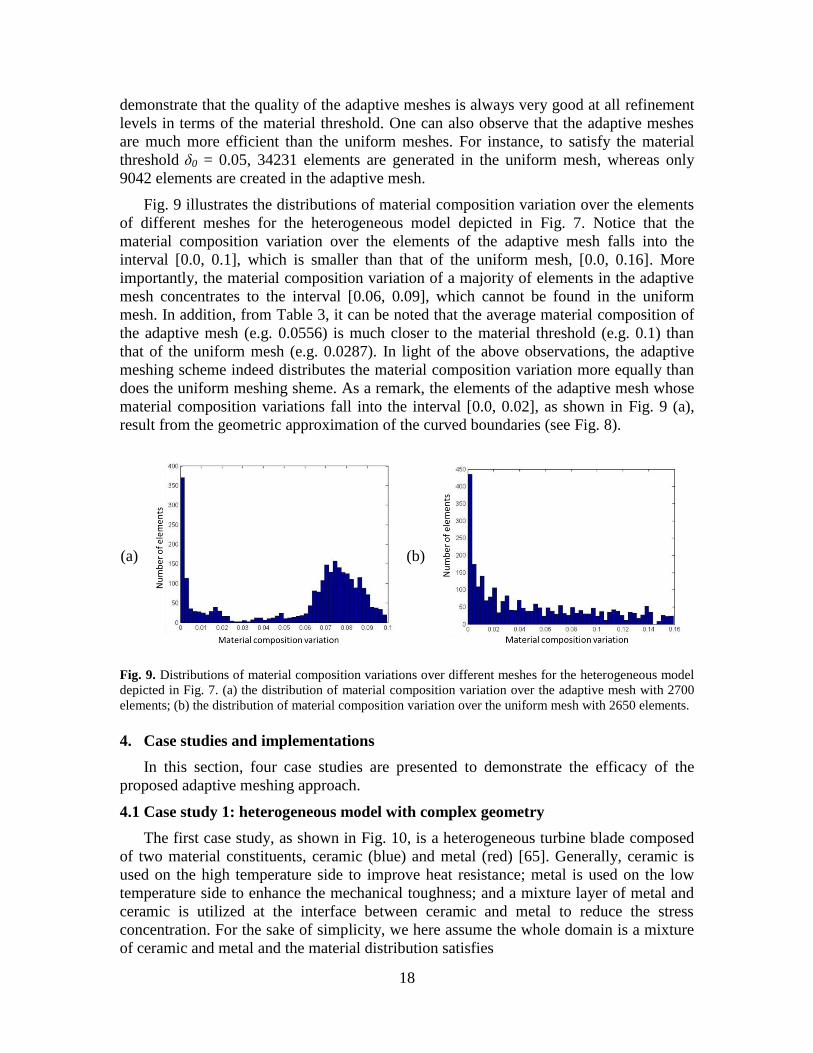
Fig. 9 illustrates the distributions of material composition variation over the elements
of different meshes for the heterogeneous model depicted in Fig. 7. Notice that the
material composition variation over the elements of the adaptive mesh falls into the
interval [0.0, 0.1], which is smaller than that of the uniform mesh, [0.0, 0.16]. More
importantly, the material composition variation of a majority of elements in the adaptive
mesh concentrates to the interval [0.06, 0.09], which cannot be found in the uniform
mesh. In addition, from Table 3, it can be noted that the average material composition of
the adaptive mesh (e.g. 0.0556) is much closer to the material threshold (e.g. 0.1) than
that of the uniform mesh (e.g. 0.0287). In light of the above observations, the adaptive
meshing scheme indeed distributes the material composition variation more equally than
does the uniform meshing sheme. As a remark, the elements of the adaptive mesh whose
material composition variations fall into the interval [0.0, 0.02], as shown in Fig. 9 (a),
result from the geometric approximation of the curved boundaries (see Fig. 8).
(a)
(b)
Fig. 9. Distributions of material composition variations over different meshes for the heterogeneous model
depicted in Fig. 7. (a) the distribution of material composition variation over the adaptive mesh with 2700
elements; (b) the distribution of material composition variation over the uniform mesh with 2650 elements.
4. Case studies and implementations
In this section, four case studies are presented to demonstrate the efficacy of the
proposed adaptive meshing approach.
4.1 Case study 1: heterogeneous model with complex geometry
The first case study, as shown in Fig. 10, is a heterogeneous turbine blade composed
of two material constituents, ceramic (blue) and metal (red) [65]. Generally, ceramic is
used on the high temperature side to improve heat resistance; metal is used on the low
temperature side to enhance the mechanical toughness; and a mixture layer of metal and
ceramic is utilized at the interface between ceramic and metal to reduce the stress
concentration. For the sake of simplicity, we here assume the whole domain is a mixture
of ceramic and metal and the material distribution satisfies

19
2
PP cddf (26)
where f is the material composition of metal, c is a constant that prevents the function
value from exceeding 1.0, and dP is the distance from an arbitrary point P to the outer
boundary C as shown in Fig. 10 (b).
Since the material composition function is analytic, we apply the algorithm described
in Section 3.2 to generate an adaptive mesh of this heterogeneous model. Fig. 10 (c)
shows the adaptive mesh where the material threshold δ0 = 0.1. As seen in Table 5 (at the
end of Section 4.3), 8301 elements are generated in the uniform mesh, whereas only 3806
elements are created in the adaptive mesh. It also can be noted from Table 5 that the
average material composition variation over the adaptive mesh (0.0413) is closer to the
material threshold than that of the uniform mesh (0.0246); the mesh quality of the
adaptive mesh (qavg = 0.915) is high and comparable to that of the uniform mesh (qavg =
0.950).
(a)
(b)
(c)
Fig. 10. The heterogeneous model and the corresponding adaptive mesh for case study 1. (a) the material
distribution; (b) geometric definitions; (c) the adaptive mesh where δ0 = 0.1.
4.2 Case study 2: heterogeneous model with both complex material gradation and
geometry
Fig. 11 shows a complex heterogeneous object based on the HFT structure. In this
case study, the HFT structure is exactly the same as that of the example in Section 3.3,

20
but the geometry is a little bit complicated. As seen in Fig. 11 (c), both boundary feature
and interface feature are composed of curves and straight lines.
Applying the adaptive meshing algorithm that has been discussed in Section 3.3, the
adaptive mesh associated with the material threshold δ0 = 0.1 is depicted in Fig. 11 (d).
As shown in Table 5, 66922 elements are generated in the uniform mesh, whereas only
9717 elements are created in the adaptive mesh. We can also note from Table 5 that the
average material composition variation over the adaptive mesh (0.0648) is much closer to
the material threshold (0.1) than that of the uniform mesh (0.0193); the mesh quality of
the adaptive mesh (qavg = 0.9122) is high and comparable to that of the uniform mesh
(qavg = 0.9608).
(a)
(b)
(c)
(d)
Fig. 11. The HFT-based heterogeneous model and the corresponding adaptive mesh for case study 2. (a)
the material distribution; (b) the HFT structure; (c) child features in the HFT structure; (d) the adaptive
mesh where δ0 = 0.1.
4.3 Case study 3: heterogeneous model with discontinuous material gradation
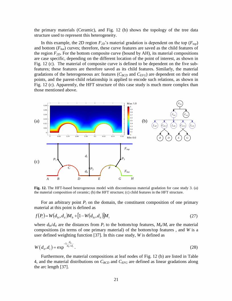
Fig. 12 shows a case study derived from [37], in which the material heterogeneity is
also represented by HFT structure. Fig. 12 (a) shows the material composition of one of
21
the primary materials (Ceramic), and Fig. 12 (b) shows the topology of the tree data
structure used to represent this heterogeneity.
In this example, the 2D region F2D’s material gradation is dependent on the top (Ftop)
and bottom (Fbot) curves; therefore, these curve features are saved as the child features of
the region F2D. For the bottom composite curve (bound by AH), its material compositions
are case specific, depending on the different location of the point of interest, as shown in
Fig. 12 (c). The material of composite curve is defined to be dependent on the five sub-
features; these features are therefore saved as its child features. Similarly, the material
gradations of the heterogeneous arc features (CBCD and CEFG) are dependent on their end
points, and the parent-child relationship is applied to encode such relations, as shown in
Fig. 12 (c). Apparently, the HFT structure of this case study is much more complex than
those mentioned above.
(a)
(b)
(c)
Fig. 12. The HFT-based heterogeneous model with discontinuous material gradation for case study 3. (a)
the material composition of ceramic; (b) the HFT structure; (c) child features in the HFT structure.
For an arbitrary point Pi on the domain, the constituent composition of one primary
material at this point is defined as
ttibibtibii MddWMddWPf ,1, (27)
where dbi/dti are the distances from Pi to the bottom/top features, Mb/Mt are the material
compositions (in terms of one primary material) of the bottom/top features , and W is a
user defined weighting function [37]. In this case study, W is defined as
5
, exp .b
b t
d
d d
b tW d d
(28)
Furthermore, the material compositions at leaf nodes of Fig. 12 (b) are listed in Table
4, and the material distributions on CBCD and CEFG are defined as linear gradations along
the arc length [37].
Ftop
Fbot db
dt P1
P2
P3
A B
C
D E
F
G H

22
Table 4
Material compositions at leaf nodes shown in Fig. 12 (b)
Location A, B D, E G, H M, N
Material composition:
[ceramic, metal] [1.00, 0.00] [0.75, 0.25] [0.50, 0.50] [0.00, 1.00]
With the material heterogeneity information defined above, the adaptive mesh
associated with the material threshold δ0 = 0.1 is generated as shown in Fig. 13. It can be
noted that several interface curves (the red ones) are embedded in the adaptive mesh at
which the material composition function is not continuous (see Fig. 12 (a)) and no
triangle elements straddle these interface curves. In this way, abrupt material composition
changes within elements are effectively avoided. As shown in Table 5, to satisfy the
material threshold δ0 = 0.1, 29758 elements are generated in the uniform mesh whereas
only 2329 elements are created in the adaptive mesh. One can also observe that the
average material composition variation over the adaptive mesh (0.0706) is much closer to
the material threshold (0.1) than that of the uniform mesh (0.0125); the mesh quality of
the adaptive mesh (qavg = 0.9376) is higher than that of the uniform mesh (qavg = 0.9217).
Fig. 13. The adaptive mesh where δ0 = 0.1 for case study 3.
Table 5 Statistics relative to the different meshing schemes for the first three case studies.
Case study Mesh type Np Ne qmin qavg δmin δavg
1 adaptive 2169 3806 0.5804 0.9150 0.0000 0.0413
uniform 4503 8301 0.2980 0.9500 0.0000 0.0246
2 adaptive 5007 9717 0.4771 0.9122 0.0000 0.0648
uniform 34035 66922 0.3793 0.9608 0.0000 0.0193
3 adaptive 1277 2329 0.4028 0.9376 0.0067 0.0706
uniform 15205 29758 0.5726 0.9217 0.0003 0.0125
4.4 Case study 4: FEA performance of the adaptive mesh
We next provide the fourth case study to illustrate the advantages of adaptive mesh
over uniform mesh in terms of FEA computational performances. In this case study, the
heterogeneous model under investigation has been shown in case study 3. Thermal-
mechanical analysis is conducted on this heterogeneous model by using the adaptive
23
mesh and uniform mesh, respectively, and FEA computational performances of both
meshes are compared.
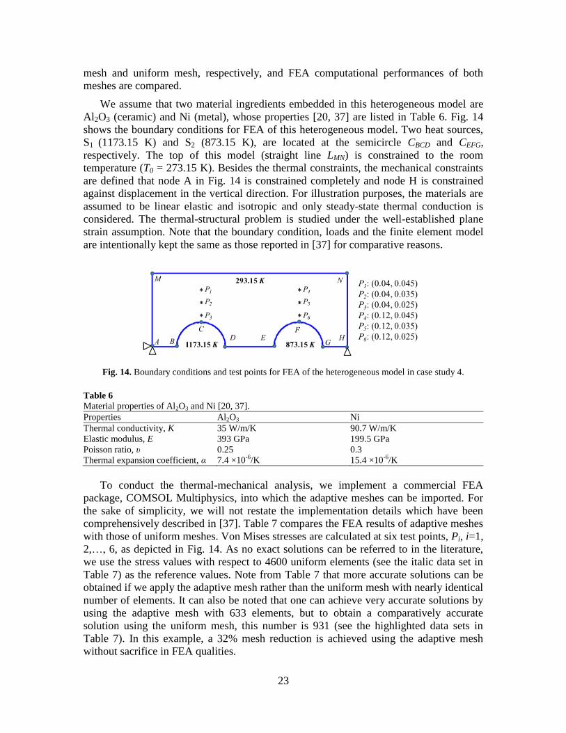
We assume that two material ingredients embedded in this heterogeneous model are
Al2O3 (ceramic) and Ni (metal), whose properties [20, 37] are listed in Table 6. Fig. 14
shows the boundary conditions for FEA of this heterogeneous model. Two heat sources,
S1 (1173.15 K) and S2 (873.15 K), are located at the semicircle CBCD and CEFG,
respectively. The top of this model (straight line LMN) is constrained to the room
temperature (T0 = 273.15 K). Besides the thermal constraints, the mechanical constraints
are defined that node A in Fig. 14 is constrained completely and node H is constrained
against displacement in the vertical direction. For illustration purposes, the materials are
assumed to be linear elastic and isotropic and only steady-state thermal conduction is
considered. The thermal-structural problem is studied under the well-established plane
strain assumption. Note that the boundary condition, loads and the finite element model
are intentionally kept the same as those reported in [37] for comparative reasons.
Fig. 14. Boundary conditions and test points for FEA of the heterogeneous model in case study 4. Table 6
Material properties of Al2O3 and Ni [20, 37].
Properties Al2O3 Ni
Thermal conductivity, K 35 W/m/K 90.7 W/m/K
Elastic modulus, E 393 GPa 199.5 GPa
Poisson ratio, υ 0.25 0.3
Thermal expansion coefficient, α 7.4 ×10⁻⁶
/K 15.4 ×10⁻⁶
/K
To conduct the thermal-mechanical analysis, we implement a commercial FEA
package, COMSOL Multiphysics, into which the adaptive meshes can be imported. For
the sake of simplicity, we will not restate the implementation details which have been
comprehensively described in [37]. Table 7 compares the FEA results of adaptive meshes
with those of uniform meshes. Von Mises stresses are calculated at six test points, Pi, i=1,
2,…, 6, as depicted in Fig. 14. As no exact solutions can be referred to in the literature,
we use the stress values with respect to 4600 uniform elements (see the italic data set in
Table 7) as the reference values. Note from Table 7 that more accurate solutions can be
obtained if we apply the adaptive mesh rather than the uniform mesh with nearly identical
number of elements. It can also be noted that one can achieve very accurate solutions by
using the adaptive mesh with 633 elements, but to obtain a comparatively accurate
solution using the uniform mesh, this number is 931 (see the highlighted data sets in
Table 7). In this example, a 32% mesh reduction is achieved using the adaptive mesh
without sacrifice in FEA qualities.

24
Table 7
FEA results of different meshing schemes at six test points.
von Mises stress
(109 N/m
2)
Number of elements (Uniform mesh) Number of elements (Adaptive mesh)
4600 931 624 456 248 633 473 252
σvP1
0.8215 0.8242 0.8239 0.8268 0.8303 0.8269 0.8272 0.8270
σvP2
1.4434 1.4471 1.4503 1.4513 1.4558 1.4468 1.4502 1.4500
σvP3
2.2174 2.2215 2.2278 2.2398 2.2529 2.2175 2.2155 2.2197
σvP4
0.5686 0.5701 0.5705 0.5726 0.5753 0.5714 0.5715 0.5780
σvP5
0.9864 0.9883 0.9895 0.9919 0.9959 0.9861 0.9881 0.9953
σvP6
1.4863 1.4887 1.4940 1.5029 1.5110 1.4880 1.4852 1.4846
5. Conclusions and discussions
Adaptive meshing for FEA of heterogeneous material objects is investigated in this
paper. The major contributions of this paper includes: the material heterogeneity
information is fully exploited in the mesh generation process, and a generic approach is
proposed to generate adaptive meshes for various types of heterogeneous material
models. Though only two types of heterogeneous objects are referred to, the proposed
adaptive meshing method is generally applicable to other heterogeneous object
representations that have been discussed in [1]. In the proposed approach, a CVT-based
method is employed to govern mesh adaptation according to a density function related to
the material distribution. Armed with such a density function, one can control the
allocation of mesh nodes to obtain an equal distribution of material composition variation
over elements and hence minimize the number of elements in terms of a predefined
material threshold. To our knowledge, there seems to be no similar methods that can
achieve such a flexible control on the adaptive mesh in the context of mesh generation of
heterogeneous materials. In addition, an adaptive sampling technique is developed to
evaluate the validity of a mesh in terms of the material threshold. In this technique, the
nodes of CVT-based meshes serve as sample points directly and thus the material
composition variation within each element is calculated by just interrogating the material
compositions at its vertices. In traditional approaches, however, substantial material
interrogations at a large number of sampling points have to be called for.
We have successfully applied the proposed approach into several benchmarking case
studies. Our numerical experiments show that the proposed approach can tackle adaptive
meshing problems for heterogeneous objects with both complex geometries and material
distributions. In particular, non-continuous material gradation problem can also be solved
by using a divide and conquer-based method. Benefiting from CVT’s superior properties,
no matter how complicated a heterogeneous model is, the proposed approach can always
generate a high quality mesh. In addition, the experiments illustrate that the proposed
approach can approximate the material distribution well (or satisfy the material threshold)
with significantly less elements compared to the uniform mesh. Finally, FEA results
demonstrate that the proposed approach can obtain significant reduction of mesh
elements without sacrifice of FEA qualities.
The proposed method currently targets at adaptive mesh generation for 2D
heterogeneous objects only and it is, however, a nontrivial task to directly extend it to
adaptive meshing of 3D heterogeneous objects, though tetrahedral mesh generation based
on CVT has been studied in [50]. The main reason is that CVT-based tetrahedral mesh
25
generation cannot fully eliminate the degenerated elements (e.g. slivers), while CVT-
based triangular meshing can always guarantee high-quality meshes (provided the input
domain has no sharp angles). In recent years, some researchers have proposed that using
Optimal Delaunay Triangulation (ODT)-based techniques (alternative to CVT-based
methods) can significantly reduce the number of slivers in the tetrahedral meshes and
thus improve the mesh quality [66, 67]. In the future work, we are going to extend the
presented approach to 3D elements in quest for adaptive tetrahedral mesh generation
methods based on ODT approaches.
Acknowledgement
The authors would like to thank the Research Grant Council of HKUSAR
Government and the Department of mechanical Engineering, the University of Hong
Kong for supporting this project [HKU717409E].
References
[1] X.Y. Kou, S.T. Tan, Heterogeneous object modeling: A review, Comput Aided Design, 39 (2007) 284-
301.
[2] A. Pasko, V. Adzhiev, P. Comninos, Heterogeneous Objects Modelling and Applications, Collection of
Papers on Foundations and Practice Series, Lecture Notes in Computer Science, 2008.
[3] V. Kumar, D. Burns, D. Dutta, C. Hoffmann, A framework for object modeling, Comput Aided Design,
31 (1999) 541-556.
[4] A.J. Markworth, K.S. Ramesh, W.P. Parks, Modelling studies applied to functionally graded materials,
Journal of Materials Science, 30 (1995) 2183-2193.
[5] M.Y. Wang, X. Wang, A level-set based variational method for design and optimization of
heterogeneous objects, Comput Aided Design, 37 (2005) 321-337.
[6] E.R. Ivar, Functionally Graded Materials, in: K.W. James (Ed.) Handbook of Advanced Materials, 2004,
pp. 465-486.
[7] F. Watari, H. Kondo, S. Matsuo, R. Miyao, A. Yokoyama, M. Omori, T. Hirai, Y. Tamura, M. Uo, N.
Ohara, T. Kawasaki, Development of functionally graded implant and dental post for bio-medical
application, Mater Sci Forum, 423-4 (2003) 321-326.
[8] J.F. Shackelford, Bioceramics: applications of ceramic and glass materials in medicine, Uetikon-
Zuerich, Switzerland: Trans Tech Publications Ltd., 1999.
[9] J.F. Li, R. Watanabe, N. Nishio, A. Kawasaki, Design and Fabrication of Diamond Tools with Ceramic
Shank Using the Concept of Functionally Gradient Materials, in: Proceedings of 1994 Powder Metallurgy
World Congress, Paris, France, 1994, pp. 553-556.
[10] C. Cline, Preparation and properties of gradient titanium carbide cermet cutting tools, Metal Powder
Report, 52 (1997) 39-39.
[11] Č. Drašar, A. Mrotzek, C. Stiewe, E. Müller, W.A. Kaysser, Developing Mechanically and Chemically
Stable Contacts between Bi2Te3 and FeSi2, Functionally Graded Materials VII, Materials Science Forum,
423-425 (2002) 391-398.
[12] Y. Liu, E.I. Meletis, Tribological behavior of DLC coatings with functionally gradient interfaces,
Surface and Coatings Technology, 153 (2002) 178-183.
[13] J. Huang, Heterogeneous component modeling and optimal design for manufacturing, PhD Thesis,
Department of Mechanical Engineering, Clemson University, 2000.
[14] X.P. Qian, D. Dutta, Physics-Based Modeling for Heterogeneous Objects, Journal of Mechanical
Design, 125 (2003) 416-427.
[15] I. Elishakoff, C. Gentilini, E. Viola, Three-dimensional analysis of an all-round clamped plate made of
functionally graded materials, Acta Mechanica, 180 (2005) 21-36.
[16] J. Huang, G.M. Fadel, V.Y. Blouin, M. Grujicic, Bi-objective optimization design of functionally
gradient materials, Materials & Design, 23 (2002) 657-666.
26
[17] A. Eraslan, T. Akis, On the plane strain and plane stress solutions of functionally graded rotating solid
shaft and solid disk problems, Acta Mechanica, 181 (2006) 43-63.
[18] J.R. Cho, S.W. Shin, Material composition optimization for heat-resisting FGMs by artificial neural
network, Composites Part A: Applied Science and Manufacturing, 35 (2004) 585-594.
[19] J. Yang, K.M. Liew, Y.F. Wu, S. Kitipornchai, Thermo-mechanical post-buckling of FGM cylindrical
panels with temperature-dependent properties, International Journal of Solids and Structures, 43 (2006)
307-324.
[20] J.R. Cho, D.Y. Ha, Optimal tailoring of 2D volume-fraction distributions for heat-resisting
functionally graded materials using FDM, Comput Method Appl M, 191 (2002) 3195-3211.
[21] J.H. Kim, G.H. Paulino, Isoparametric graded finite elements for nonhomogeneous isotropic and
orthotropic materials, J Appl Mech-T Asme, 69 (2002) 502-514.
[22] G. Zhao, H. Zhang, L. Cheng, Geometry-adaptive generation algorithm and boundary match method
for initial hexahedral element mesh, Engineering with Computers, 24 (2008) 321-339.
[23] T. Plewa, T.J. Linde, T. Linde, V.G. Weirs, Adaptive mesh refinement, theory and applications, Berlin:
Springer, 2005.
[24] S.H. Lo, Finite element mesh generation and adaptive meshing, Progress in Structural Engineering and
Materials, 4 (2002) 381-399.
[25] J. Ruppert, A Delaunay Refinement Algorithm for Quality 2-Dimensional Mesh Generation, J
Algorithm, 18 (1995) 548-585.
[26] J.R. Shewchuk, Triangle: Engineering a 2D Quality Mesh Generator and Delaunay Triangulator,
in: Applied computational geometry towards geometric engineering, 1996, pp. 203-222.
[27] S.H. Lo, New mesh generation scheme for arbitrary planar domains, International Journal for
Numerical Methods in Engineering, 21 (1985) 1403-1426.
[28] R. Lohner, P. Parikh, Generation of three-dimensional unstructured grids by the advancing-front
method, International Journal for Numerical Methods in Fluids, 8 (1988) 1135-1149.
[29] M.A. Yerry, M.S. Shephard, Automatic three-dimensional mesh generation by the modified-octree
technique, International Journal for Numerical Methods in Engineering, 20 (1984) 1965-1990.
[30] M.A. Yerry, M.S. Shephard, Modified quadtree approach to finite element mesh generation, IEEE
Computer Graphics and Applications, 3 (1983) 39-46.
[31] N.P. Weatherill, O. Hassan, Efficient 3-Dimensional Delaunay Triangulation with Automatic Point
Creation and Imposed Boundary Constraints, International Journal for Numerical Methods in Engineering,
37 (1994) 2005-2039.
[32] T.S. Lau, S.H. Lo, Finite element mesh generation over analytical curved surfaces, Comput Struct, 59
(1996) 301-309.
[33] W.H. Friey, Selective refinement: A new strategy for automatic node placement in graded triangular
meshes, International Journal for Numerical Methods in Engineering, 24 (1987) 2183-2200.
[34] J.M. Sullivan, G. Charron, K.D. Paulsen, A three-dimensional mesh generator for arbitrary multiple
material domains, Finite Elements in Analysis and Design, 25 (1997) 219-241.
[35] P.H. Schimpf, D.R. Haynor, Y. Kim, Object-free adaptive meshing in highly heterogeneous 3-D
domains, International Journal of Bio-Medical Computing, 40 (1996) 209-225.
[36] A. Nikbakht, M. Sadighi, A.F. Arezoodar, Indentation of a transversely loaded functionally graded
rectangular plate by a rigid spherical indentor, P I Mech Eng C-J Mec, 227 (2013) 663-682.
[37] X.Y. Kou, S.T. Tan, A systematic approach for integrated computer-aided design and finite element
analysis of functionally-graded-material objects, Materials & Design, 28 (2007) 2549-2565.
[38] G. Giunta, S. Belouettar, E. Carrera, Analysis of FGM Beams by Means of Classical and Advanced
Theories, Mech Adv Mater Struc, 17 (2010) 622-635.
[39] S.H. Chi, Y.L. Chung, Mechanical behavior of functionally graded material plates under transverse
load - Part II: Numerical results, International Journal of Solids and Structures, 43 (2006) 3675-3691.
[40] K.H. Shin, Adaptive mesh generation for finite element analysis of functionally graded materials, in:
American Society of Mechanical Engineers, Computers and Information in Engineering Division, CED,
Orlando, FL, 2005, pp. 199-206.
[41] X.Y. Kou, S.T. Tan, W.S. Sze, Modeling complex heterogeneous objects with non-manifold
heterogeneous cells, Comput Aided Design, 38 (2006) 457-474.
[42] X.Y. Kou, S.T. Tan, A hierarchical representation for heterogeneous object modeling, Comput Aided
Design, 37 (2005) 307-319.

27
[43] W.K. Chiu, X.Y. Kou, S.T. Tan, Adaptive meshing of 2D heterogeneous objects using material
quadtree, Computer-Aided Design & Applications, 8 (2011) 289-300.
[44] J.R. Shewchuk, What Is a Good Linear Element? Interpolation, Conditioning, and Quality Measures,
in: Proceedings of the 11th International Meshing Roundtable, Sandia National Laboratories, 2002, pp.
115–126.
[45] G.H. Paulino, J.H. Kim, The weak patch test for nonhomogeneous materials modeled with graded
finite elements, Journal of the Brazilian Society of Mechanical Sciences and Engineering, 29 (2007) 63-81.
[46] Q. Du, V. Faber, M. Gunzburger, Centroidal Voronoi tessellations: Applications and algorithms, Siam
Rev, 41 (1999) 637-676.
[47] Q. Du, M. Gunzburger, L.L. Ju, Advances in Studies and Applications of Centroidal Voronoi
Tessellations, Numer Math-Theory Me, 3 (2010) 119-142.
[48] Q. Du, M. Gunzburger, Grid generation and optimization based on centroidal Voronoi tessellations,
Appl Math Comput, 133 (2002) 591-607.
[49] Q. Du, M.D. Gunzburger, L.L. Ju, Constrained centroidal Voronoi tessellations for surfaces, Siam J
Sci Comput, 24 (2003) 1488-1506.
[50] Q. Du, D.S. Wang, Tetrahedral mesh generation and optimization based on centroidal Voronoi
tessellations, International Journal for Numerical Methods in Engineering, 56 (2003) 1355-1373.
[51] Q. Du, D.S. Wang, Recent progress in robust and quality Delaunay mesh generation, J Comput Appl
Math, 195 (2006) 8-23.
[52] L.L. Ju, Conforming centroidal Voronoi Delaunay triangulation for quality mesh generation, Int J
Numer Anal Mod, 4 (2007) 531-547.
[53] H. Nguyen, J. Burkardt, M. Gunzburger, L. Ju, Y. Saka, Constrained CVT meshes and a comparison
of triangular mesh generators, Comp Geom-Theor Appl, 42 (2009) 1-19.
[54] L.L. Ju, M. Gunzburger, W.D. Zhao, Adaptive finite element methods for elliptic PDEs based on
conforming centroidal Voronoi-Delaunay triangulations, Siam J Sci Comput, 28 (2006) 2023-2053.
[55] Y.Q. Huang, H.F. Qin, D.S. Wang, Q. Du, Convergent Adaptive Finite Element Method Based on
Centroidal Voronoi Tessellations and Superconvergence, Commun Comput Phys, 10 (2011) 339-370.
[56] J. Chen, D. Wang, Q. Du, Linear finite element superconvergence on simplicial meshes, Mathematics
of Computation, 83 (2014) 2161-2185.
[57] Y.Q. Huang, H.F. Qin, D.S. Wang, Centroidal Voronoi tessellation-based finite element
superconvergence, International Journal for Numerical Methods in Engineering, 76 (2008) 1819-1839.
[58] W. Quadros, V. Vyas, M. Brewer, S. Owen, K. Shimada, A computational framework for automating
generation of sizing function in assembly meshing via disconnected skeletons, Engineering with Computers,
26 (2010) 231-247.
[59] W.R. Quadros, Computational Framework for Generating 3D Finite Element Mesh Sizing Function
via Skeleton, PhD Thesis, Carnegie Mellon University, 2005.
[60] W.R. Quadros, S.J. Owen, M.L. Brewer, K. Shimada, Finite Element Mesh Sizing for Surfaces Using
Skeleton, in: Proceedings of the 13th International Meshing Roundtable, 2004, pp. 389-400.
[61] J. Tournois, P. Alliez, O. Devillers, Interleaving Delaunay Refinement and Optimization for 2D
Triangle Mesh Generation, in: Proceedings of the 16th International Meshing Roundtable, 2008, pp. 83-101.
[62] D.A. Field, Quantitative measures for initial meshes, International Journal for Numerical Methods in
Engineering, 47 (2000) 887-906.
[63] M. Nemat-Alla, N. Noda, Edge crack problem in a semi-infinite FGM plate with a bi-directional
coefficient of thermal expansion under two-dimensional thermal loading, Acta Mechanica, 144 (2000) 211-
229.
[64] X.Y. Kou, Computer-Aided Design of Heterogeneous Objects, PhD Thesis, Department of Mechanical
Engineering, The University of Hong Kong, 2005.
[65] X.P. Qian, D. Dutta, Design of heterogeneous turbine blade, Comput Aided Design, 35 (2003) 319-
329.
[66] P. Alliez, D. Cohen-Steiner, M. Yvinec, M. Desbrun, Variational tetrahedral meshing, Acm T Graphic,
24 (2005) 617-625.
[67] J. Tournois, C. Wormser, P. Alliez, M. Desbrun, Interleaving Delaunay Refinement and Optimization
for Practical Isotropic Tetrahedron Mesh Generation, Acm T Graphic, 28 (2009).