FINITE ELEMENT CENTER - CiteSeerX

FINITE ELEMENT CENTER

PREPRINT 2003–18

CAD-to-CAE integration through automated modelsimplification and adaptive modelling

K.Y. Lee, M.A. Price, C.G. Armstrong,M.G. Larson, and K. Samuelsson

Chalmers Finite Element CenterCHALMERS UNIVERSITY OF TECH-NOLOGYGoteborg Sweden 2003

CHALMERS FINITE ELEMENT CENTER

Preprint 2003–18

CAD-to-CAE integration through automatedmodel simplification and adaptive modelling

K.Y. Lee, M.A. Price, C.G. Armstrong,M.G. Larson, and K. Samuelsson

Chalmers Finite Element CenterChalmers University of Technology

SE–412 96 Goteborg SwedenGoteborg, October 2003

CAD-to-CAE integration through automated model simplification and adaptive mod-ellingK.Y. Lee, M.A. Price, C.G. Armstrong,M.G. Larson, and K. SamuelssonNO 2003–18ISSN 1404–4382

Chalmers Finite Element CenterChalmers University of TechnologySE–412 96 GoteborgSwedenTelephone: +46 (0)31 772 1000Fax: +46 (0)31 772 3595www.phi.chalmers.se

Printed in SwedenChalmers University of TechnologyGoteborg, Sweden 2003

International Conference on Adaptive Modeling and Simulation ADMOS 2003

N.-E Wiberg and P. Díez (Eds) CIMNE, Barcelona, 2003

CAD-TO-CAE INTEGRATION THROUGH AUTOMATED MODEL SIMPLIFICATION AND ADAPTIVE MODELLING

K.Y. Lee*, M. A. Price#, C. G. Armstrong*, M. Larson† and K. Samuelsson† *School of Mechanical and Manufacturing

Queen’s University Belfast Belfast UK BT9 5AH

e-mail: [email protected], [email protected] web page: http://www.fem.qub.ac.uk

School of Aeronautical Engineering Queen’s University Belfast

Belfast UK BT9 5AG e-mail: [email protected] web page: http://www.fem.qub.ac.uk

† Chalmers Finite Element Center

Chalmers University Email: [email protected] [email protected]

Key words: Model Simplification, Medial Axis Transform, Medial Axis, Adaptive Modelling, Sub-Modelling.

Abstract. Virtual prototyping through simulation is being widely adopted as part of the product design cycle. However, designers often find themselves crippled by the limitation of exiting technologies when dealing with real world CAD models. CAD models often contain details for aesthetic and manufacturing purposes which are irrelevant or even harmful to the analysis. It is always a tedious and time consuming task to clean-up CAD geometry in preparation for mesh generation. Typically the designer will perform a preliminary analysis to evaluate every possible high-risk region in the conceptual design and then improve the design and rerun the analysis for confirmation. This iterative practice is extremely time consuming and labour intensive for a complicated model; for example a gearbox assembly will typically has 2,000,000~2,500,000 DOF. Unfortunately it is also critical for designer to follow this approach in order to fine-tune their designs.

It is the aim of this research to fuse the gaps in current practices and technologies for a seamless integration of the CAD-to-CAE process. A series of algorithmic procedures for small feature identification is presented. The Medial Axis Transform (MAT) is used in these procedures to provide geometric proximity information. When used in conjunction with global

1

mailto:[email protected]


http://www.fem.qub.ac.uk/



International Conference on Adaptive Modeling and Simulation ADMOS 2003

N.-E Wiberg and P. Díez (Eds) CIMNE, Barcelona, 2003

tolerances, the simplification process can be orchestrated to cater for different types of models and account for relative size of the feature. Model simplification enables the designer to create a coarsest possible mesh for an efficient preliminary analysis.

Coarse mesh enables analysts shorten the analysis time, and identify “hot” spots from the analysis results more quickly. Most of these “hot” spots will require a much finer mesh to capture their true local behaviour. This paper will also provide an intuitive method for mesh refinement while respecting the original CAD geometries.

2

K. Y. Lee, M. A. Price, C. G. Armstrong, M. Larson and K. Samuelsson

1 INTRODUCTION The analysis process is a key part of the product design cycle. The analysis performed on

the initial conceptual design provides feedback regarding the product’s functional behaviour. Should these results indicate any unpredicted behaviour in the product, appropriate changes will be made to rectify flaws so that it will perform as specified. This is an ideal situation where the analysis process was carried out simultaneously with the design process.

In early generations of analysis systems, analysts would build the mesh using a bottom-up approach to form a mesh that approximates the target geometry. It is only since CAD systems started to mature that top-down meshing approaches, where mesh algorithms operate on a geometrical model, became the norm. As CAD models become more complex, these geometry based meshing methods enabled analysts to reuse the CAD geometry in order to save time. However, the idea of sharing and reusing CAD data for CAE purpose has numerous obstacles preventing it from being a smooth transition. As CAD and CAE are two different systems each evolved from different background to cater for different needs, which in turn resulted in a different terminology and data representations. As a result, attempts to integrate CAD and CAE processes always introduce a chain of problems that need to be rectified before the CAD data is suitable for the analysis purpose.

Previous researches on CAD and CAE integration have focused on developing new tools for geometry and topology editing. Butlin et al i and Jones et al ii demonstrated a strategy in deriving a valid CAE model through geometry editing. As most of the standard CAD exchange formats used do not contain sufficient information or incorrect tolerances lead to incomplete model representation in the target systems, it is often necessary to perform certain degree of geometric editing such as collapse, replacement, regeneration etc to ensure, for examples a 3D geometry is defined by a completely closed surface. More recently, Ribó et aliii showed a similar approach in order to derive a valid CAE model. The results of the previous researches have been implemented in commercial product like CADfixiv and Gidv respectively. Nonetheless geometric editing can be very computationally intensive as it often involves recalculating new definitions to replace original geometries that are unsuitable for analysis purposes. To avoid this computational expensive step, Sheffer et alvi, vii and Armstrong et al viii,ix proposed a new algorithm to approach the model simplification process. This new algorithm introduces an additional layer of new topology on top of the original model to resolve spurious definitions and simplifying the model’s topological definitions. As topology or connectivity of the model entities in a model database can be easily modified, it is considerable more efficient in utilizing computational resources. While other contemporary work from Shephard et alxand Fine et alxi demonstrated another approaches. The suggested algorithm simply avoiding the geometry and topology editing of the model itself, it achieves a reasonable mesh by manipulating the surface mesh of the model. It uses element size and mesh quality to control what sort of small feature will be represented during the analysis or being suppressed.

3


2 CAD-TO-CAE INTEGRATION The present of these geometric editing tools has made the CAD data reusability in analysis

a more practical approach and closing the gap of errors during data transfer between different systems. Nonetheless, numerous geometric issues in generating a CAE model from CAD within a rapid design cycle remain to be addressed.

During the integration of CAD and CAE processes, numerous problems arise, hindering the attempts in creating a seamless design chain processes from design to analysis. The obstacles are varying across different scenarios in different industries, but they can be categorised into two main groups according to their nature and cause of the obstacles. Following sections will describe the major obstacles according to their natures.

2.1 CAD-to-CAE data exchange Reusing the CAD data in an analysis can be done by transferring data through a neutral

format to the target systems or accessing the CAD data directly through a set of CAD systems’ API.

Exporting CAD data in a readable and standard format to the target systems is the most adopted practice nowadays in transferring data between CAD and CAE systems. Neutral formats were designed so that a model created in one package can be easily read by other CAD/CAE systems. The three basic neutral formats are STEP, IGES and STL. This transfer process merely taken care of geometry entities delivery “as is”, i.e. every entity in the source system is transfer to an identical entity in the target systems or converted into some similar entity. For example, surfaces are converted into NURBS representation with a specified tolerance deviation from its original shape.

In terms of neutral formats, CAD translation is required to convert the original CAD model to the neutral format. During any form of translation there is scope for data to be misinterpreted and badly translated. The standards (IGES and STEP) are open to individual interpretation. As a result, although based on a common definition, both STEP and IGES translators vary greatly from vendor to vendor in terms of how they define the standard rules. Systems will also have varying levels of support for the range of entities in a given standard. All of this gives rise to potential problems in the translation process, especially when undertaken fully automatic data translation.

STEP (STandard for the Exchange of Product model data) is an ISO standard that translates individual solids and entire assemblies, while maintaining the assembly structure and positioning of components within an assembly. Parametric information, including features, colours, and layers is lost during a translation, but the ability to translate as a solids eliminates at least half of the cleanup work currently required when using alternative translation methods. STEP uses a data definition language called EXPRESS - this is both human and machine-readable (like XML) and therefore has a single, unique interpretation - this makes it very powerful.

Since the inception of IGES (Initial Graphics Exchange Specification), it has been

4


developed into a well supported, mature and robust specification. It is an ANSI-approved standard format that is used with 3D wire frame models. It is now at release 5.3 - which may be its last as STEP is gradually taking over, however, it is far from dead. IGES file specification is detailed in a manual of over 620 pages, many of which detail countless numbers of different geometric entities and attributes. The specification is used for the description of 3D polygonal and NURB geometry, B-Rep geometry, 2D entities such as lines, hatch symbols, text entities, etc. IGES solid entities are only supported by a few CAD systems so people that attempt to use IGES to exchange solid models usually export the model as a set of trimmed surface entities. Therefore, if you use IGES for exchange, the conversion process will usually involve some sort of model healing that involves substituting alternative IGES entities, stitching up gaps between surfaces and re-computing intersections to repair geometric inaccuracies.

STL was a format that was designed for Stereo lithography applications such as rapid prototyping. The format simply contains a triangulation of the outer surfaces so it just consists of a collection of triangles. Specialist capability is required to convert this surface mesh into a volume mesh, and as there is not geometry associated with the file format, one cannot apply loads or boundary conditions to the geometric features such as an edge or face as analysts would usually do when geometry is available. This format should really only be used as the last resort.

Proprietary kernel file formats are also used for data exchange purposes although not as common as neutral file formats. These are software libraries that are used to store the CAD model details and operate on the model's features. Every CAD system is built on top of some type of kernel - the kernel carries out the geometric operations such as creating entities, features and carrying out Booleans. The most common kernel formats are Parasolid and ACIS. As each CAD system is built on top of a kernel, each system can usually export files in the underlying kernel format (X_T for Parasolid, SAT for ACIS). Pre-processors can usually read all neutral formats, at least one form of kernel format and if they have an agreement with a CAD vendor (becoming more common), they can read CAD native formats too.

In short, exchanging data through intermediate file format tends to have certain unfavourable outcomes because of following issues:

• Inconsistencies in the file exchange format (STEP, IGES, VDAFS, ACIS, Parasolid)

• Mismatched tolerances in different systems.

• Inconsistencies in both geometric and topological representation between source CAD systems and target analysis systems.

All these data exchange issues generally lead to problems such as duplicate entities, gaps in curves and surfaces in analysis systems, and even incomplete models at the receiving end.

Certain CAE packages provide the capability to read in major CAD systems native binary file format without going through intermediate file format. This approach alleviates most of

5


the problematic introduced when exchanging data through intermediate file, provided the target system is able to manipulate the original geometry entities and not converting them implicitly.

Access to information in a CAD model can also be done through access routines or API, ambiguities in data representation can be avoided in addition it also enable analyst to modify design parameters within the CAE environment. It is this uniqueness in communication that drawn the attention of most analysts, for analysis to be an efficient tool within the design process, analyst must be allowed to explore different model specification based on a previous analysis result. Hence the key components in this analysis driven design cycle is the ability to manipulate geometry from within CAE environment.

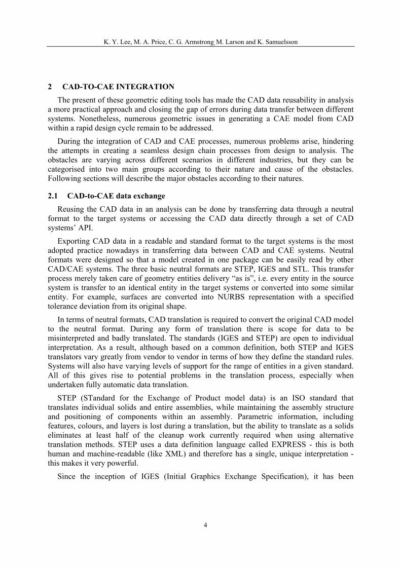
The Object Management Group, Inc. (OMG) has defined an interface standard for CAD systems that enable the interoperability of CAD, CAM and CAE tools. This interface, CADServices is intents to establish a series of high-level engineering queries, and avoid many of the problems associated with data translation. This is achieved through the provision of CORBA interfaces with consistent functionality across native CAD implementations. To an extent, all queries use native CAD system geometry kernels and associated software as shown in Figure 1. This neutral standard interface has already attracted attentions from software vendors; a commercial implementation of CADServices is CADScript from TranscenData.

CADServices Architecture

Client Client Client Application A Application B Application C

CADServices

Unigraphics Pro/ENGINEER CATIA I-DEAS STEP/IGES

Figure 1 Illustration of CADServices being used as a neutral interface to native CAD geometry kernel

2.2 Complex geometry The quality of the mesh during an analysis affects the analysis quality, speed of analysis

and above all its appropriateness for simulating the original design intent. It is vital that analysts can generate a mesh from CAD geometry both efficiently and accurately. However, for analysts the successful reception of a CAD model does not mean the model is ready to be meshed “as is”. This can be because the model created by the designer is often not the appropriate model representation required by the analysis. For instance, structural analysis of an aircraft structure often required dimensional reduction to be performed on the 3D detailed

6


model. Idealisation of the 3D models to lower dimensional elements like beams, shells, or plates is often necessary to reflect the true physical functional behaviour of the models in real world environment.

On the other hand, CAD models often contain details for aesthetic and manufacturing purposes which are totally irrelevant to the analysis. Irrelevant details can also including those features which have no significant effect on the global model analysis but are critical in analysing its locality behaviour. It is widely known that a realistic-scale CAD model very often consists hundred or even thousand of surfaces that are not suitable for FEA mesh generation. For such a model, mesh generation is not a process of discretisation that divides all these trimmed surface patches into small elements. On the contrary, elements should be used to plate across features below the element size. This is necessary because on such cases, if the previous approach was not taken excessive nodes will be placed around these small features for conformity by the auto mesher and will result in low-quality mesh elements.

The problems discussed above must be overcome in designing a CAD-to-CAE integration system. Tools develop to tackle these problematic geometric issues have to be as neutral as possible so that they can be deployed in different CAE system. Following sections will outline the effort taken within this research to reach this goal.

2.3 Model operators Preparing a CAD model for the analysis often involves the editing processes. These editing

processes are designed to derive a clean model, which is free of irrelevant details, also as symmetrical as possible, so that existing meshing algorithms can proceed with mesh generation. Conventional pre-processor package, like CADfix, will pursuit this editing task using the “hard” geometric approach, where any unsuitable geometric entities are replace with newly computed geometric entities. However, this is not the only approach in deriving a suitable CAE model for analysis. Fluent Inc. pre-processor: GAMBIT adopted Sheffer et alvi approach in addition of the conventional hard geometric approach. In this research a hierarchical approach were suggested to solve this problem. It is based on layers of tools:

a) a low layer of a repertoire of ‘atomic’ functions for finding individual features and modifying them.

b) a top layer of wizard scripts that orchestrate a sequence of the low layer functions to achieve an automatic, as far as is possible, defeaturing of a whole model to suit a specified purpose, such as convert a CAD model of a complex mechanical component to ensure successful automatic and relevantly economic meshing of that part.

Hence this work presents a generic model simplification approach that a set of algorithmic procedure was designed to target small features starting from a lower dimension and propagating toward 3D. This approach gives the analyst the following advantages:

1) Most small features introduce undesirable elements at surface mesh level

7


2) Eliminating small feature at lower dimensional level is less computational intensive

3) Achieving a good quality surface mesh help reduce problems in volume mesh generation.

However it is the aim of this research to provide a group of open geometric operators which are implementation-independent and representation-independent. Before proceed to describe these geometric operators, a couple of terminology will be introduced and used.

A target is a term used to describe a geometric entity that will be subject to any geometric operators, while tool is the term used within this thesis to describe the resulting entities created from any geometric operators.

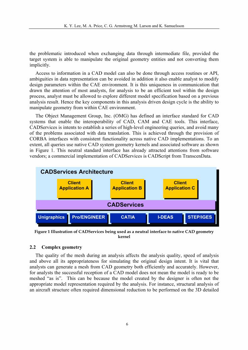
2.3.1 Merge The merge operator allows adjacent entities with identical dimension and geometric

properties to be merged into one. If entities of similar dimension and of similar geometric properties; for instance, straight line, curve, arc, etc. for edges; can be merge into a single entity provided they are within user specified tolerance.

One of the commonly used file format protocol in data exchange, IGES, usually does not provide topological connectivity information. Instead it leaves it to the receiving end to reconstruct the topology from the geometry. Therefore, duplicate entities are very common after data exchange process. To reconstruct the topology, the merge operator can be used to search out duplicate entities and annihilate them by replacing them with a single and unambiguous entity.

The new entity, tool, to replace the designated duplicate entities, target, will be of similar dimension and geometric properties. While the precise location of this new entity will depends on user choice. It can either be an average location computed from target or a designated location specified by the user.

ε

tool target

Figure 2 Merge: similar target entities were being merged into one entity, tool

8


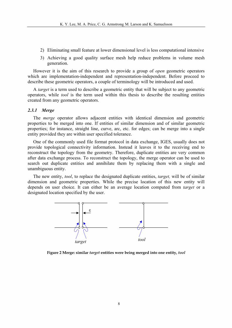
2.3.2 Split Any entity within a model except point can be split into two or more entity of similar

dimension by introducing one or more entities of lower dimension. Entities are split by lower dimension entities, so that an edge is split by a vertex, a face by an edge, and a body by a face. The splitting entity is constrained to lie within the parent entity, so that an edge partitioning a face lies on the face.

Tool: split lines used to the face

Figure 3 Split: A face split by additional lines (left), new faces created as a result (right)

2.3.3 Insert The insert command allows the definition or modification of target, a general bounded

line, surface or body. This is a very general command, and does not check that the target defined is meaningful. This means that it can be used to define any lines, surfaces or bodies. Logically, one would expect the boundary lines of a surface to join up into loops so that regions of finite area are trimmed off. In fact, the insert command allows the definition of surfaces whose boundaries are not connected, and whose areas are not finite.

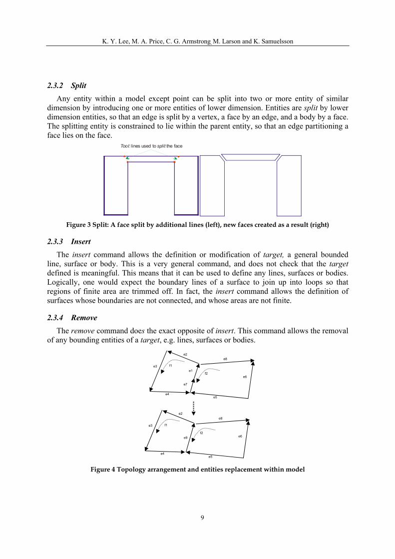
2.3.4 Remove The remove command does the exact opposite of insert. This command allows the removal

of any bounding entities of a target, e.g. lines, surfaces or bodies.

e2

Figure 4 Topology arrangement and entities replacement within model

e3

e8

f1 e1

f2 e6

e7

e4 e5

e2 e8

f1 e3

f2 e6 e9

e4 e5

9


In Figure 4, f1 is a simple face which is formed by a closed loop of edge lines e1, e2, e3, e4 and e7, which are fully connected end to end. The orientation of each of these lines from its start point to its end point is indicated by the arrows on the lines. Lines e1 and e7 can be replaced with a single line to simplify the model’s definition. Hence, the first step involves is to remove the target, e1 & e7, and then insert tool, e9, as shown in Figure 4.

2.4 Orchestrating Model Simplification Previous sections described a selection of common geometric operators that most analysts

would use from a day to day basic during pre-processing. They may appear under a different name or with a different appearance on different packages but under the hood the functionalities remain the same.

Preparing a model for meshing is always a tedious and time consuming task due to the various reasons discussed before. Even with the introductory of easy to use and fast operators like those described in section before will not help to improve the task efficiency if analysts don’t know where and when to apply these tools. Much of the previous research focuses were on deriving new geometric editing operators whilst little attention were paid on finding the problems in CAD model in the first place.

The following sections will attempt to address this issue by providing a few find algorithms together with their corresponding fixer using the low-level geometric operator discussed above. A list of commonly found small features within CAD models that are not specific to any industries’ practices had been identified, namely:

1. faceted edges 2. sliver edges 3. constriction areas 4. patches of surfaces

These small features do not typically fall into standard categories that can be explicitly identified and suppressed by the algorithms proposed in Li et al xii and Zhu et al xiii, which do not identify sliver edges, sliver faces and narrow regions.

2.4.1 Faceted Edges It is common for CAD data to contain unwanted topology that has been introduced during

the model creation process, but is not essential to the form of the object being modelled. The existence of segmented edges may result in more elements being required to respect the model boundary than is necessary for a conforming representation of the model. This can be rectified by searching through the model for a group of edges that are tangentially continuous and have common vertices with a connectivity of two. The group of line segments can then be replaced by a single edge. When a chain of edges is joined the individual edges are sampled and a new single edge is fitted through sample points.

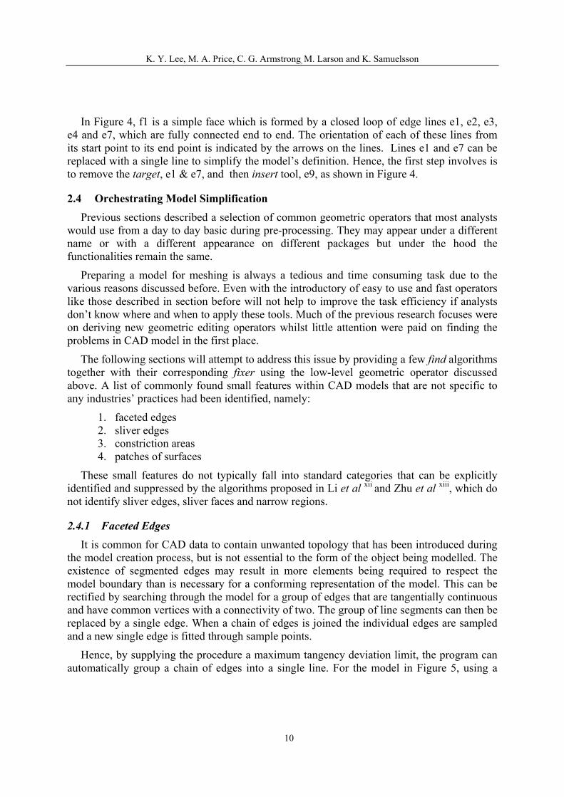
Hence, by supplying the procedure a maximum tangency deviation limit, the program can automatically group a chain of edges into a single line. For the model in Figure 5, using a

10


limit of 5º, the number of lines in the model can be reduced from 702 to 232 without changes to the original geometric shapes..

Figure 5 Faceted edges (hidden lines) in a CATIA v4 generated model

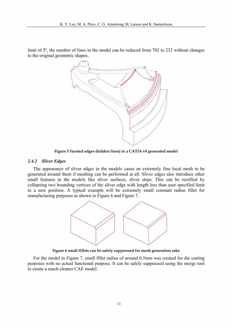
2.4.2 Sliver Edges The appearance of sliver edges in the models cause an extremely fine local mesh to be

generated around them if meshing can be performed at all. Sliver edges also introduce other small features in the models like sliver surfaces, sliver steps. This can be rectified by collapsing two bounding vertices of the sliver edge with length less than user specified limit to a new position. A typical example will be extremely small constant radius fillet for manufacturing purposes as shown in Figure 6 and Figure 7.

Figure 6 small fillets can be safely suppressed for mesh generation sake

For the model in , small fillet radius of around 0.5mm was created for die casting purposes with no actual functional purpose. It can be safely suppressed using the merge tool to create a much cleaner CAE model.

Figure 7

11


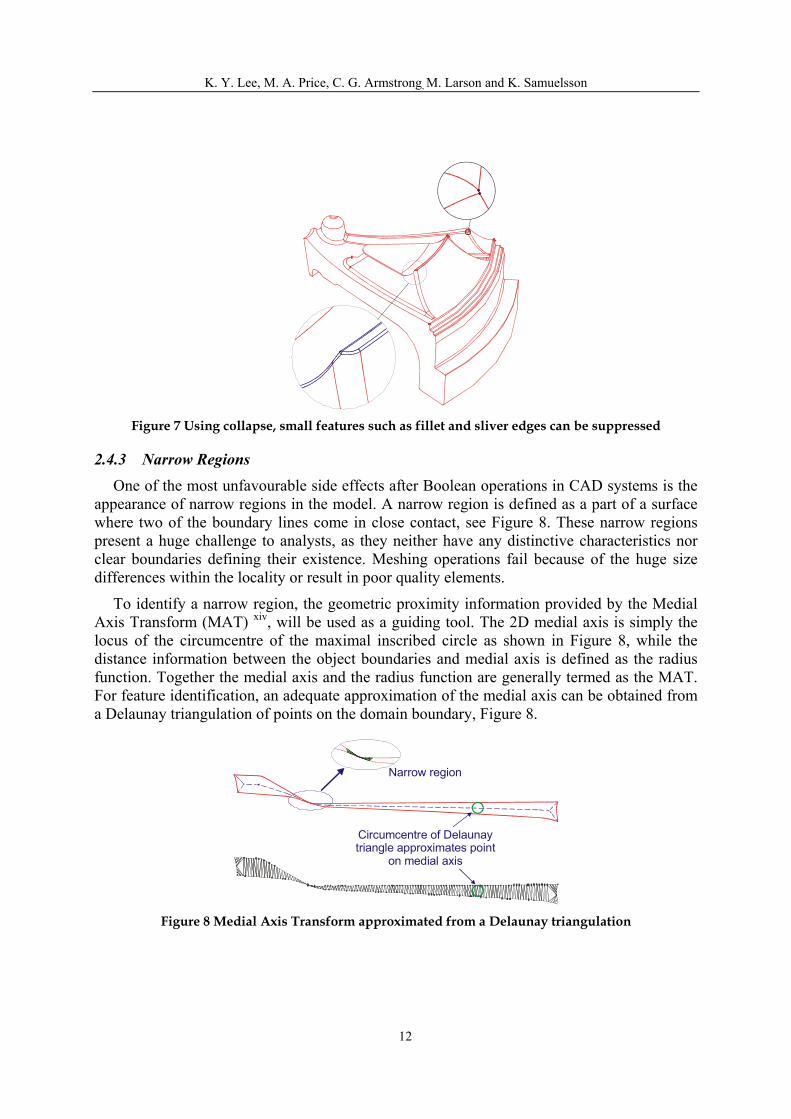
Figure 7 Using collapse, small features such as fillet and sliver edges can be suppressed

2.4.3 Narrow Regions One of the most unfavourable side effects after Boolean operations in CAD systems is the

appearance of narrow regions in the model. A narrow region is defined as a part of a surface where two of the boundary lines come in close contact, see Figure 8. These narrow regions present a huge challenge to analysts, as they neither have any distinctive characteristics nor clear boundaries defining their existence. Meshing operations fail because of the huge size differences within the locality or result in poor quality elements.

To identify a narrow region, the geometric proximity information provided by the Medial Axis Transform (MAT) xiv, will be used as a guiding tool. The 2D medial axis is simply the locus of the circumcentre of the maximal inscribed circle as shown in Figure 8, while the distance information between the object boundaries and medial axis is defined as the radius function. Together the medial axis and the radius function are generally termed as the MAT. For feature identification, an adequate approximation of the medial axis can be obtained from a Delaunay triangulation of points on the domain boundary, Figure 8.

Circumcentre of Delaunaytriangle approximates point

on medial axis

Narrow region

Figure 8 Medial Axis Transform approximated from a Delaunay triangulation

12


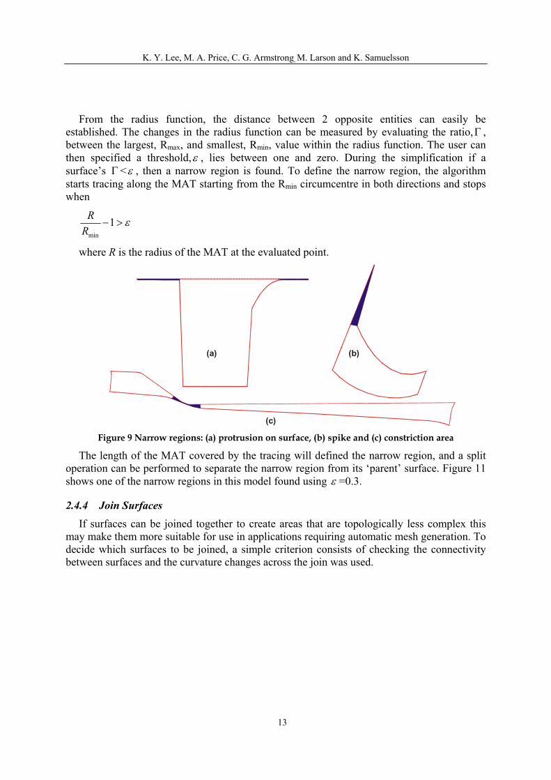
From the radius function, the distance between 2 opposite entities can easily be established. The changes in the radius function can be measured by evaluating the ratio,Γ , between the largest, Rmax, and smallest, Rmin, value within the radius function. The user can then specified a threshold,ε , lies between one and zero. During the simplification if a surface’s <Γ ε , then a narrow region is found. To define the narrow region, the algorithm starts tracing along the MAT starting from the Rmin circumcentre in both directions and stops when

ε>−1minRR

where R is the radius of the MAT at the evaluated point.

(a) (b)

(c) Figure 9 Narrow regions: (a) protrusion on surface, (b) spike and (c) constriction area

The length of the MAT covered by the tracing will defined the narrow region, and a split operation can be performed to separate the narrow region from its ‘parent’ surface. Figure 11 shows one of the narrow regions in this model found using ε =0.3.

2.4.4 Join Surfaces If surfaces can be joined together to create areas that are topologically less complex this

may make them more suitable for use in applications requiring automatic mesh generation. To decide which surfaces to be joined, a simple criterion consists of checking the connectivity between surfaces and the curvature changes across the join was used.

13


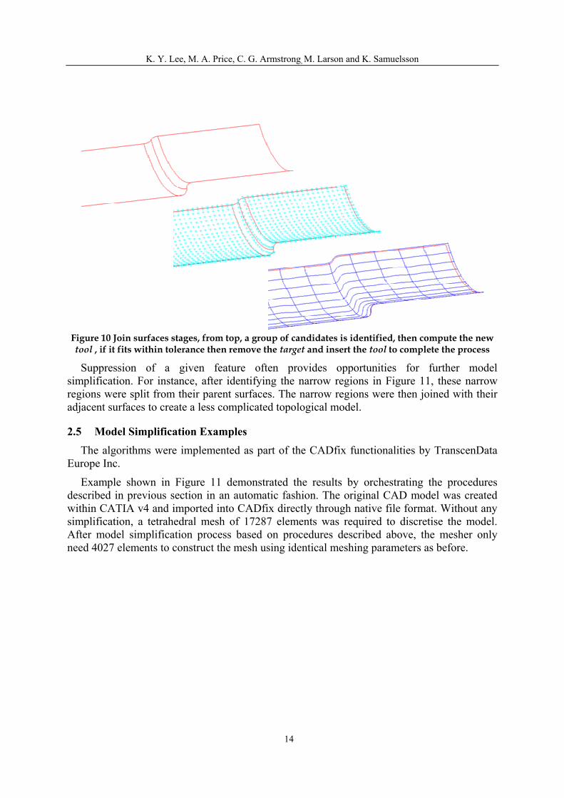
Figure 10 Join surfaces stages, from top, a group of candidates is identified, then compute the new tool , if it fits within tolerance then remove the target and insert the tool to complete the process

Suppression of a given feature often provides opportunities for further model simplification. For instance, after identifying the narrow regions in , these narrow regions were split from their parent surfaces. The narrow regions were then joined with their adjacent surfaces to create a less complicated topological model.

Figure 11

2.5 Model Simplification Examples The algorithms were implemented as part of the CADfix functionalities by TranscenData

Europe Inc.

Example shown in Figure 11 demonstrated the results by orchestrating the procedures described in previous section in an automatic fashion. The original CAD model was created within CATIA v4 and imported into CADfix directly through native file format. Without any simplification, a tetrahedral mesh of 17287 elements was required to discretise the model. After model simplification process based on procedures described above, the mesher only need 4027 elements to construct the mesh using identical meshing parameters as before.

14


Facet Edges

Narrow Region

0.11m

Sliver Edges,Sliver Surface

Surfaces joined

m

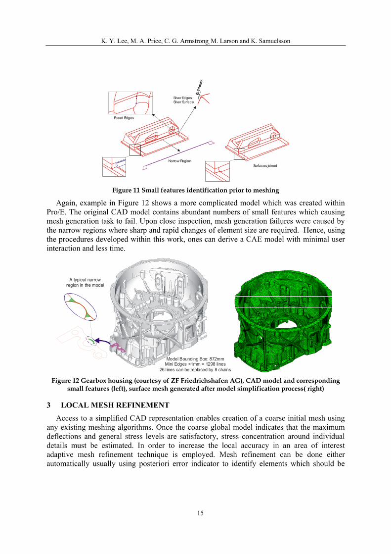
Figure 11 Small features identification prior to meshing

Again, example in Figure 12 shows a more complicated model which was created within Pro/E. The original CAD model contains abundant numbers of small features which causing mesh generation task to fail. Upon close inspection, mesh generation failures were caused by the narrow regions where sharp and rapid changes of element size are required. Hence, using the procedures developed within this work, ones can derive a CAE model with minimal user interaction and less time.

A typical narrow region in the model

Model Bounding Box: 872mmMini Edges <1mm = 1298 lines

26 lines can be replaced by 8 chains Figure 12 Gearbox housing (courtesy of ZF Friedrichshafen AG), CAD model and corresponding

small features (left), surface mesh generated after model simplification process( right)

3 LOCAL MESH REFINEMENT Access to a simplified CAD representation enables creation of a coarse initial mesh using

any existing meshing algorithms. Once the coarse global model indicates that the maximum deflections and general stress levels are satisfactory, stress concentration around individual details must be estimated. In order to increase the local accuracy in an area of interest adaptive mesh refinement technique is employed. Mesh refinement can be done either automatically usually using posteriori error indicator to identify elements which should be

15


refined or interactively refine the mesh. In the latter case the user defines a region of particular interest where the mesh should be refined, for instance, the vicinity of a high stress concentration in a solid mechanics simulation. Improved local accuracy can be obtained either by solving a global problem on the locally refined mesh or by solving only a local problem on the refined sub-domain, a technique called sub-modelling.

3.1 Mesh refinement respecting the CAD geometry When performing mesh refinement it is of fundamental importance that the refinement

process takes the true CAD geometry into account. Otherwise user will in general not obtain the desired increase in accuracy. In fact, spurious stress concentrations may occur in the vicinity of artificial non convex corners when the mesh is refined.

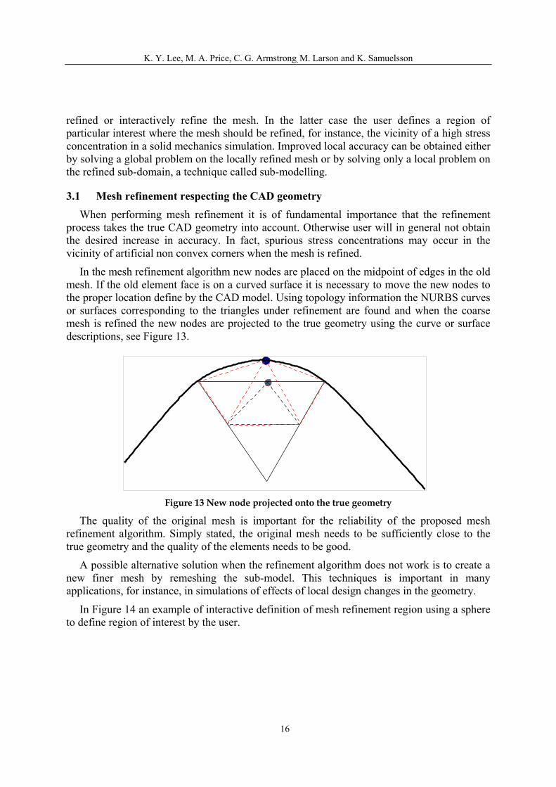
In the mesh refinement algorithm new nodes are placed on the midpoint of edges in the old mesh. If the old element face is on a curved surface it is necessary to move the new nodes to the proper location define by the CAD model. Using topology information the NURBS curves or surfaces corresponding to the triangles under refinement are found and when the coarse mesh is refined the new nodes are projected to the true geometry using the curve or surface descriptions, see Figure 13.

Figure 13 New node projected onto the true geometry

The quality of the original mesh is important for the reliability of the proposed mesh refinement algorithm. Simply stated, the original mesh needs to be sufficiently close to the true geometry and the quality of the elements needs to be good.

A possible alternative solution when the refinement algorithm does not work is to create a new finer mesh by remeshing the sub-model. This techniques is important in many applications, for instance, in simulations of effects of local design changes in the geometry.

In Figure 14 an example of interactive definition of mesh refinement region using a sphere to define region of interest by the user.

16


Figure 14 Local mesh refinement respecting CAD geometries, mesh refinement were carried out on

elements enclosed within the wire-frame sphere

Figure 15 The resulting mesh after three levels of refinement

17


4 CONCLUSIONS AND FUTURE WORK At this early stage of the research, all the key procedures are applied in sequence to

achieve model simplification. It is envisaged that a more novel macro-like script will be developed in the future to orchestrate the simplification process. Nevertheless, tests carried out on both relatively simple and complex real world models indicated a dramatic reduction in preparation time prior to mesh. The model simplification strategy proposed here also managed to reduce the element numbers by 76% in the simple model in , simplified the complex model in Figure 12 from an unmeshable state to meshable.

Figure 11

The procedures developed so far have been concentrated on making a model meshable on a general basis. Nonetheless, these procedures are designed to rectify the most common problems faced by analysts on a daily basis. As new or existing procedures can be added/removed from the orchestrated simplification process, it provides a framework which can adapt to different modelling and analysis scenarios and eventually lead to a full automation of the model simplification task.

With the intuitive mesh refinement method presented in this work, analysts can easily refine their initial coarse mesh adaptively at regions of interest. The next natural step in the development of these techniques is to construct efficient finite element algorithms for computation of locally enhanced solutions. A simple and fast technique is sub-modeling. The basic steps in an interactive sub-modelling algorithm are:

• Solve the global problem on a coarse mesh. • Define the region of interest. • Create a refined mesh respecting the true CAD geometry in the defined region. The

refined mesh may be obtained by refinement or remeshing. • Define suitable boundary conditions using the global coarse mesh solution. For

instance, in a solid mechanics computation the boundary conditions may be the displacements on the boundary of the region of interest.

• Solve the local finite element problem on the region of interest.

Sub-modelling techniques provide rapid algorithms which normally run in real time allowing interactive exploration of for instance local design changes.

There are three sources of error in the sub-modelling algorithm

• The error in the boundary conditions obtained from the coarse mesh. • The error in the finite element solution on the refined region of interest. • The error in the approximation of geometry.

Balancing these three errors is an intricate task crucial to the design of sub-modelling algorithms. It is planned to address these issues in future work.

18


19

REFERENCES i Butlin G., Stops C. CAD data repair. Proc. 5th International Meshing Roundtable. 1996; pp 7-12, ii Jones M.R, Price M.A, Butlin G. Geometry management Support for Auto-Meshing. Proc. 4th

International Meshing Roundtable Conference, 1995; pp 153-164. iii Ribó R., Bugeda G., Onate E. Some algorithms to correct a geometry in order to create a finite element

mesh. Computer-Aided Design 2002; 80:1399-1408 iv http://www.cadfix.com v http://gid.cimne.upc.es/index.html vi Sheffer A, Blacker T, Bercovier M. Virtual Topology Operators for Meshing. International Journal of

Computational Geometry and Applications 2000; 10(3): 309-331 vii Sheffer A. Model Simplification for Meshing Using Face Clustering. Computer-Aided Design 2001;

33:925-934 viii Armstrong C.G, Robinson D.J, McKeag R.M, Li T.S, Bridgett S.J, Donaghy R.J, McGleenan C.A.

Medials for meshing and more. Proc. 4th International Meshing Roundtable 1995; pp277-288 ix Armstrong C.G, Bridgett S.J, Donaghy R.J, McCune R.W, McKeag R.M, Robinson D.J. Techniques for

Interactive and Automatic Idealisation of CAD Models. Numerical Grid Generation in Computational Field Simulations, Ed. M. Cross., B. K. Soni, J. F. Thompson, J. Hauser, P. R. Eiseman, Proceedings of the 6th International Conference, held at the University of Greenwich, pp 643-662, July 1998

x Shephard M.S, Beall M.W, O’Bara R.M, “Revisiting the Elimination of the Adverse Effects of Small Model Features in Automatically Generated Meshes", Proceedings, 7th International Meshing Roundtable, Sandia National Lab, pp.119-132, 1998

xi Fine L, Remondini L, Leon J-C, “Automated generation of FEA models through idealization operators”, Int. J. Numerical Method End. 2000; 49:83-108

xii Li B, Liu J. Detail feature recognition and decomposition in solid model. Computer-Aided Design 2002; 34:405-414

xiii Zhu H, Menq C.H. B-REP model simplification by automatic fillet/round suppressing for efficient automatic feature recognition. Computer-Aided Design 2002; 34:109-123

xiv Sheehy D.J, Armstrong C.G, Robinson D.J. Computing the medial surface of a solid from a domain Delaunay triangulation. ACM Symposium on Solid Modeling Foundations and Applications 1995; pp 201-212.

http://www.cadfix.com/

1

Chalmers Finite Element Center Preprints

2001–01 A simple nonconforming bilinear element for the elasticity problemPeter Hansbo and Mats G. Larson

2001–02 The LL∗ finite element method and multigrid for the magnetostatic problemRickard Bergstrom, Mats G. Larson, and Klas Samuelsson

2001–03 The Fokker-Planck operator as an asymptotic limit in anisotropic mediaMohammad Asadzadeh

2001–04 A posteriori error estimation of functionals in elliptic problems: experimentsMats G. Larson and A. Jonas Niklasson

2001–05 A note on energy conservation for Hamiltonian systems using continuous timefinite elementsPeter Hansbo

2001–06 Stationary level set method for modelling sharp interfaces in groundwater flowNahidh Sharif and Nils-Erik Wiberg

2001–07 Integration methods for the calculation of the magnetostatic field due to coilsMarzia Fontana

2001–08 Adaptive finite element computation of 3D magnetostatic problems in potentialformulationMarzia Fontana

2001–09 Multi-adaptive galerkin methods for ODEs I: theory & algorithmsAnders Logg

2001–10 Multi-adaptive galerkin methods for ODEs II: applicationsAnders Logg

2001–11 Energy norm a posteriori error estimation for discontinuous Galerkin methodsRoland Becker, Peter Hansbo, and Mats G. Larson

2001–12 Analysis of a family of discontinuous Galerkin methods for elliptic problems:the one dimensional caseMats G. Larson and A. Jonas Niklasson

2001–13 Analysis of a nonsymmetric discontinuous Galerkin method for elliptic prob-lems: stability and energy error estimatesMats G. Larson and A. Jonas Niklasson

2001–14 A hybrid method for the wave equationLarisa Beilina, Klas Samuelsson and Krister Ahlander

2001–15 A finite element method for domain decomposition with non-matching gridsRoland Becker, Peter Hansbo and Rolf Stenberg

2001–16 Application of stable FEM-FDTD hybrid to scattering problemsThomas Rylander and Anders Bondeson

2001–17 Eddy current computations using adaptive grids and edge elementsY. Q. Liu, A. Bondeson, R. Bergstrom, C. Johnson, M. G. Larson, and K.Samuelsson

2001–18 Adaptive finite element methods for incompressible fluid flowJohan Hoffman and Claes Johnson

2001–19 Dynamic subgrid modeling for time dependent convection–diffusion–reactionequations with fractal solutionsJohan Hoffman

2

2001–20 Topics in adaptive computational methods for differential equationsClaes Johnson, Johan Hoffman and Anders Logg

2001–21 An unfitted finite element method for elliptic interface problemsAnita Hansbo and Peter Hansbo

2001–22 A P 2–continuous, P 1–discontinuous finite element method for the Mindlin-Reissner plate modelPeter Hansbo and Mats G. Larson

2002–01 Approximation of time derivatives for parabolic equations in Banach space:constant time stepsYubin Yan

2002–02 Approximation of time derivatives for parabolic equations in Banach space:variable time stepsYubin Yan

2002–03 Stability of explicit-implicit hybrid time-stepping schemes for Maxwell’s equa-tionsThomas Rylander and Anders Bondeson

2002–04 A computational study of transition to turbulence in shear flowJohan Hoffman and Claes Johnson

2002–05 Adaptive hybrid FEM/FDM methods for inverse scattering problemsLarisa Beilina

2002–06 DOLFIN - Dynamic Object oriented Library for FINite element computationJohan Hoffman and Anders Logg

2002–07 Explicit time-stepping for stiff ODEsKenneth Eriksson, Claes Johnson and Anders Logg

2002–08 Adaptive finite element methods for turbulent flowJohan Hoffman

2002–09 Adaptive multiscale computational modeling of complex incompressible fluidflowJohan Hoffman and Claes Johnson

2002–10 Least-squares finite element methods with applications in electromagneticsRickard Bergstrom

2002–11 Discontinuous/continuous least-squares finite element methods for elliptic prob-lemsRickard Bergstrom and Mats G. Larson

2002–12 Discontinuous least-squares finite element methods for the Div-Curl problemRickard Bergstrom and Mats G. Larson

2002–13 Object oriented implementation of a general finite element codeRickard Bergstrom

2002–14 On adaptive strategies and error control in fracture mechanicsPer Heintz and Klas Samuelsson

2002–15 A unified stabilized method for Stokes’ and Darcy’s equationsErik Burman and Peter Hansbo

2002–16 A finite element method on composite grids based on Nitsche’s methodAnita Hansbo, Peter Hansbo and Mats G. Larson

2002–17 Edge stabilization for Galerkin approximations of convection–diffusion prob-lemsErik Burman and Peter Hansbo

3

2002–18 Adaptive strategies and error control for computing material forces in fracturemechanicsPer Heintz, Fredrik Larsson, Peter Hansbo and Kenneth Runesson

2002–19 A variable diffusion method for mesh smoothingJ. Hermansson and P. Hansbo

2003–01 A hybrid method for elastic wavesL.Beilina

2003–02 Application of the local nonobtuse tetrahedral refinement techniques nearFichera-like cornersL.Beilina, S.Korotov and M. Krızek

2003–03 Nitsche’s method for coupling non-matching meshes in fluid-structure vibrationproblemsPeter Hansbo and Joakim Hermansson

2003–04 Crouzeix–Raviart and Raviart–Thomas elements for acoustic fluid–structureinteractionJoakim Hermansson

2003–05 Smoothing properties and approximation of time derivatives in multistep back-ward difference methods for linear parabolic equationsYubin Yan

2003–06 Postprocessing the finite element method for semilinear parabolic problemsYubin Yan

2003–07 The finite element method for a linear stochastic parabolic partial differentialequation driven by additive noiseYubin Yan

2003–08 A finite element method for a nonlinear stochastic parabolic equationYubin Yan

2003–09 A finite element method for the simulation of strong and weak discontinuitiesin elasticityAnita Hansbo and Peter Hansbo

2003–10 Generalized Green’s functions and the effective domain of influenceDonald Estep, Michael Holst, and Mats G. Larson

2003–11 Adaptive finite element/difference method for inverse elastic scattering wavesL.Beilina

2003–12 A Lagrange multiplier method for the finite element solution of elliptic domaindecomposition problems using non-matching meshesPeter Hansbo, Carlo Lovadina, Ilaria Perugia, and Giancarlo Sangalli

2003–13 A reduced P 1–discontinuous Galerkin methodR. Becker, E. Burman, P. Hansbo, and M. G. Larson

2003–14 Nitsche’s method combined with space–time finite elements for ALE fluid–structure interaction problemsPeter Hansbo, Joakim Hermansson, and Thomas Svedberg

2003–15 Stabilized Crouzeix–Raviart element for the Darcy-Stokes problemErik Burman and Peter Hansbo

2003–16 Edge stabilization for the generalized Stokes problem: a continuous interiorpenalty methodErik Burman and Peter Hansbo

2003–17 A conservative flux for the continuous Galerkin method based on discontinuousenrichmentMats G. Larson and A. Jonas Niklasson

These preprints can be obtained from

www.phi.chalmers.se/preprints

FINITE ELEMENT CENTER - CiteSeerX

Documents

Transcript of FINITE ELEMENT CENTER - CiteSeerX