Nonlinear Finite Element Analysis of Shrinking Reinforced ...
124
DEGREE PROJECT IN CIVIL ENGINEERING AND URBAN MANAGEMENT, SECOND CYCLE, 30 CREDITS STOCKHOLM, SWEDEN 2018 Nonlinear Finite Element Analysis of Shrinking Reinforced Concrete Slabs-on-ground SHRUTHI PRAKASH KTH ROYAL INSTITUTE OF TECHNOLOGY SCHOOL OF ARCHITECTURE AND THE BUILT ENVIRONMENT
-
Upload
khangminh22 -
Category
Documents
-
view
1 -
download
0
Transcript of Nonlinear Finite Element Analysis of Shrinking Reinforced ...

DEGREE PROJECT IN CIVIL ENGINEERING AND URBAN MANAGEMENT,SECOND CYCLE, 30 CREDITSSTOCKHOLM, SWEDEN 2018
Nonlinear Finite Element Analysis of Shrinking Reinforced Concrete Slabs-on-ground
SHRUTHI PRAKASH
KTH ROYAL INSTITUTE OF TECHNOLOGYSCHOOL OF ARCHITECTURE AND THE BUILT ENVIRONMENT


Nonlinear Finite Element Analysis ofShrinking Reinforced ConcreteSlabs-on-ground
Shruthi Prakash
Master Thesis in Concrete Structures, June 2018TRITA-ABE-MBT-18299ISBN 978-91-7729-868-7

c©Shruthi Prakash 2018KTH Royal Institute of TechnologyDepartment of Civil and Architectural EngineeringDivision of Concrete StructuresStockholm, Sweden, 2018

Abstract
Concrete slabs-on-ground are commonly used in many types of industrial floors,warehouses, highways, parking lots and buildings. Cracks and deflection of slabsare undesired events caused by differential shrinkage, which limits the service life ofthe slabs. Non-linear behavior of cracks and deflections, interaction of concrete andreinforcement increase the complexity in predicting the occurrence and positioningof cracks. The Eurocode 2 provides a reference for theoretical approximation fordesign of concrete structures. This thesis intent to investigate the crack behavior ofslabs-on-ground subjected to gradient shrinkage using nonlinear finite element anal-ysis, as implemented in the software package Atena 2D. The first part of the thesis isfocused on suitable modeling techniques for predicting cracks in concrete slabs-on-ground due to gradient shrinkage. The second part is directed towards parametricstudies, performed to explore the significance of varying thickness, length, concretestrength class, bond types, reinforcement content and friction coefficient. The re-sults obtained with the Atena 2D was validated using the design software WIN-statikfor calculating the maximum crack width in the context of obtaining realistic re-sults. Finally, the WSP guide recommended parameters were tested as inputs to themodel. A slab-on-ground was modeled in Atena 2D considering these as staticallyindeterminate structures, where both slab and grade were included and the conver-gence analysis performed under plane stress conditions enabling prediction of themaximum crack widths for increasing applied shrinkage loads. Parametric studiesdemonstrate the dependency of the slab length, showing that a smaller length re-duces the crack width, since such a slab is less constrained by the sub-base. To avoidcracks in the slabs their relative thickness should not be increased above a certainthickness, instead the reinforcement content should be increased. The numericalsimulation shows that different concrete strength classes give similar cracks widths.Sand as sub-base provides less crack widths for interface materials EPS, sand andgravel. Although, dry sand as interface material gives similar crack widths as EPS,it is the best to use EPS that is also used to retard the moisture diffusion fromthe sub-base. The numerical model developed was validated for the recommendedvalues given by the WSP guide, which gives less crack widths and deflections. Thenumerical model gives less crack widths compared to the Eurocode 2, which consid-ers only the statistically determinant problems overestimating the crack widths. Thepresented examples demonstrate that the developed model can accurately predictcrack formation, crack behavior and vertical deflection in concrete slabs-on-groundsubjected to gradient shrinkage loads.
iii

iv
Sammanfattning
Betongplattor används i många typer av industriella golv, lagerbyggnader, motorvä-gar och bostadshus. Sprickor, krökningar och deformation av plattor är oönskadehändelser som orsakas av differenskrympning, vilket begränsar plattornas livslängd.Icke-linjärt beteende av sprickor och krökningar, växelverkan mellan betong ocharmering ökar komplexiteten i att kunna förutsäga förekomst och läge för sprick-bildning. Eurokod 2 ger vägledning för teoretiska approximationer vid konstruk-tion av betongstrukturer. Föreliggande examensarbete syftar till att undersökasprickbeteendet hos plattor på mark utsatt för gradientkrympning, med icke-linjäranalys så som detta implementeras i analysprogrammet Atena 2D. Arbetets förstadel fokuserar på lämpliga modelleringstekniker för att förutsäga sprickor i betong-plattor på mark, orsakat av gradientkrympning. Den andra delen är inriktad påparametriska studier för att undersöka betydelsen av varierande tjocklek, längd, be-tonghållfasthetsklass, bindningstyp till underlaget, armeringsinnehåll och friktion-skoefficient. Resultaten erhållna med Atena 2D validerades med hjälp av konstruk-tionsprogrammet WIN-statik för beräkning av maximal sprickbredd för att verifieraatt realistiska resultat nåddes. Slutligen testades de av WSP-guiden rekommender-ade parametrarna som indata till modellen. En platta på mark modellerades i Atena2D under antagande om denna som statiskt obestämd struktur där både platta ochunderlaget inkluderades och där en konvergensanalys genomfördes under antagandeom under plana spännings för hållanden vilket möjliggjorde förutsägelse av de max-imala sprickbredderna orsakade av vald krympningsgradient. Parametriska studiervisar på ett beroende av plattlängd, så att en kortare längd minskar sprickbred-den, eftersom plattan då är relativt mindre rörelseförhindrad av undergrunden. Föratt undvika sprickor i plattorna bör deras relativa tjocklek inte ökas över en visstjocklek, istället bör armeringen ökas. Den numeriska simuleringen visar att olikabetonghållfasthetsklasser ger liknande sprickbredder. Sand som undergrund ger min-dre sprickbredder för gränsytor mot EPS, sand och grus. Även med torr sand somgränssnittsmaterial fås liknande sprickbredder som med EPS. Dock är det bäst attanvända EPS som också samtidigt fungerar som fuktisolering och därvid ytterligareminskar sprickorna på grund av gradientkrympning. Den utvecklade numeriska mod-ellen validerades för de rekommenderade värden som ges av WSP guiden, vilket gerberäkningsmässigt mindre sprickbredder och krökningar. Den numeriska modellenger mindre sprickbredder jämfört med Eurokod 2, som endast beaktar det statisktbestämda fallet, då de beräknade sprickbredderna generellt blir överskattade. Depresenterade exemplen visar att den utvecklade modellen möjliggör förutsägelse avsprickbildning, sprickbeteende och vertikal krökningar i betongplattor på mark ut-satta för gradientkrympnings belastningar.
v

vi

Preface
This master thesis was written as a part of the master program for the departmentof Civil and Architectural Engineering, KTH Royal Institute of Technology. Thethesis work was carried out in WSP Stockholm during the spring semester of 2018.
I would like to express my gratitude to my supervisor professor Anders Ansell forhis guidance, advice, and constructive feedback and also for helping me to organizemy work efficiently. I would like to thank my co-supervisor adjunct professor MikaelHallgren (KTH & Tyrens AB) for his time and interesting discussion on the finiteelement software Atena 2D and guidance.
I would like to thank WSP supervisor Dr. Kent Arvidsson for his great supervision,innovative ideas, guidance, discussion and great interest throughout the work. Aspecial thanks to Gruppchef Mr. Sanjeewa Withana for providing me an oppor-tunity to carry out my thesis work in his group at WSP. Also, for the interestingdiscussions, project follow up and support.
I would like to express my gratitude to Dr. Dobromil Pryl, who helped me tounderstand the technical details of the Atena 2D software throughout my thesis andfor being patiently answering several of my questions. Thanks Dr. Jan Cervenkafor giving discount on the Atena 2D software for this thesis work.
Finally, I would like to thank my parents, family, friends and beloved husbandDr. Harisha Ramachandraiah for all their support and care.
Stockholm, June 2018
Shruthi Prakash
vii


Symbols
Latin upper case letters
Ac Concrete area
As Reinforcement area
C Cohesion
D Global nodal deflection
Ecm Modulus of elasticity
Eeff Effective elastic modulus
Eps Initial strain
Ec(28) 28 days tangent value of elastic modulus
Es Elastic modulus of steel
GF0 Base value of fracture energy
GF Fracture energy
Kgob Global stiffness matrix
K Stress intensity factor
Knn Normal stiffness
Ktt Tangential stiffness
ix

N Normal force
R Restraining degree
S Total stiffness of supports
Srm Crack spacing
Wk Crack width
Latin lower case letters
b Width of slab
c Cover of slab
d Effective depth of cross section
dmax Aggregate size
fck,cube Cube strength
fck Characteristic cylinder strength
fcm Mean compressive strength
fcteff Effective tensile strength
fctm Mean tensile strength
fcu Mean cube compression strength
fy Yield strength of steel
h Height of the slab
heff Effective height of slab
h0 Notional size of concrete
kloc Local stiffness matrix
x

k1 Coefficient for bond properties of bonded reinforcement
k2 Coefficient for distribution of strain
kh Coefficient depending on notional size
kt Factor dependent on duration of load
le Element size
l Length of element
re Element load
t Age of concrete at the moment considered
ts Age of concrete at the beginning of drying shrinkage
u Perimeter part of cross section exposed to drying
Greek lower case letters
εca Autogenous shrinkage strain
εcd Drying shrinkage strain
εcm Mean strain concrete between cracks
εcs Free shrinkage strain
εcs0 Final free shrinkage strain of material
εsm Mean strain in reinforcement
µ Coefficient of friction
Φc Creep coefficient
YRH Factor to account for surrounding humidity
Yt Factor controlling time of influence
xi

αe Ratio of elastic modulus of steel to concrete modulus of elasticity
αt Coefficient of thermal expansion
βds Coefficient used to calculate drying shrinkage
∆ε Difference of strain in steel and concrete
φ Diameter of the bar
ρpeff Reinforcement ratio
σs Stress in the tension reinforcement
τ Bond stress
υ Poissons ratio
Ys Specific material weight
xii

Contents
1 Introduction 1
1.1 Background . . . . . . . . . . . . . . . . . . . . . . . . . . . . . . . . 1
1.2 Problem description . . . . . . . . . . . . . . . . . . . . . . . . . . . . 2
1.3 Aim and objectives . . . . . . . . . . . . . . . . . . . . . . . . . . . . 2
1.4 Limitations and assumptions . . . . . . . . . . . . . . . . . . . . . . . 3
1.5 Outline of the report . . . . . . . . . . . . . . . . . . . . . . . . . . . 3
2 Theory, guidelines and standards 5
2.1 Slabs-on-ground . . . . . . . . . . . . . . . . . . . . . . . . . . . . . . 5
2.2 Concrete materials . . . . . . . . . . . . . . . . . . . . . . . . . . . . 6
2.2.1 Restraining forces in concrete structures . . . . . . . . . . . . 7
2.2.2 Friction . . . . . . . . . . . . . . . . . . . . . . . . . . . . . . 9
2.3 Insulating polystyrene interface . . . . . . . . . . . . . . . . . . . . . 10
2.4 Shrinkage . . . . . . . . . . . . . . . . . . . . . . . . . . . . . . . . . 11
2.4.1 Plastic shrinkage . . . . . . . . . . . . . . . . . . . . . . . . . 12
2.4.2 Autogenous shrinkage . . . . . . . . . . . . . . . . . . . . . . 13
2.4.3 Carbonation shrinkage . . . . . . . . . . . . . . . . . . . . . . 13
2.4.4 Drying shrinkage . . . . . . . . . . . . . . . . . . . . . . . . . 14
2.5 Creep . . . . . . . . . . . . . . . . . . . . . . . . . . . . . . . . . . . 16
2.6 Cracking in concrete . . . . . . . . . . . . . . . . . . . . . . . . . . . 17
2.6.1 Curling . . . . . . . . . . . . . . . . . . . . . . . . . . . . . . 19
2.6.2 Fracture energy . . . . . . . . . . . . . . . . . . . . . . . . . . 20
2.7 Crack width according to Eurocode 2 . . . . . . . . . . . . . . . . . . 21
xiii

2.8 Calculations of crack width according to WIN-statik . . . . . . . . . . 23
3 Non-linear finite element analysis 25
3.1 Finite element analysis . . . . . . . . . . . . . . . . . . . . . . . . . . 25
3.2 Non-linear analysis . . . . . . . . . . . . . . . . . . . . . . . . . . . . 27
3.2.1 Iterative procedure . . . . . . . . . . . . . . . . . . . . . . . . 27
3.2.2 Fracture mechanics . . . . . . . . . . . . . . . . . . . . . . . . 29
3.3 Nonlinear finite element analysis using Atena 2D . . . . . . . . . . . . 30
3.3.1 Concrete modeling in Atena 2D . . . . . . . . . . . . . . . . . 30
3.3.2 Concrete cracking . . . . . . . . . . . . . . . . . . . . . . . . . 32
3.4 Reinforcement material model . . . . . . . . . . . . . . . . . . . . . . 34
3.5 Interface material . . . . . . . . . . . . . . . . . . . . . . . . . . . . . 36
3.6 Sub-base material property . . . . . . . . . . . . . . . . . . . . . . . . 37
3.7 Boundary conditions and loads . . . . . . . . . . . . . . . . . . . . . 37
4 Numerical Examples 39
4.1 Modeling approach . . . . . . . . . . . . . . . . . . . . . . . . . . . . 39
4.2 Convergence analysis . . . . . . . . . . . . . . . . . . . . . . . . . . . 40
4.2.1 Plane stress . . . . . . . . . . . . . . . . . . . . . . . . . . . . 42
4.2.2 Plane strain . . . . . . . . . . . . . . . . . . . . . . . . . . . . 44
4.3 Model check and analysis method . . . . . . . . . . . . . . . . . . . . 45
4.3.1 Model check . . . . . . . . . . . . . . . . . . . . . . . . . . . . 45
4.3.2 Analysis method . . . . . . . . . . . . . . . . . . . . . . . . . 48
4.4 Parametric study . . . . . . . . . . . . . . . . . . . . . . . . . . . . . 49
4.4.1 Varying slab length . . . . . . . . . . . . . . . . . . . . . . . . 50
4.4.2 Varying slab thickness . . . . . . . . . . . . . . . . . . . . . . 51
4.4.3 Concrete strength class . . . . . . . . . . . . . . . . . . . . . . 53
4.4.4 Reinforcement content . . . . . . . . . . . . . . . . . . . . . . 56
4.4.5 Bond definition . . . . . . . . . . . . . . . . . . . . . . . . . . 59
4.4.6 Fracture energy . . . . . . . . . . . . . . . . . . . . . . . . . . 61
xiv

4.4.7 Varying sub-base . . . . . . . . . . . . . . . . . . . . . . . . . 63
4.4.8 Effect of external load with different sub-base . . . . . . . . . 67
4.5 Parameters according to WSP guide inputs . . . . . . . . . . . . . . . 69
5 Discussion 77
6 Conclusion and further research 83
6.1 Conclusion . . . . . . . . . . . . . . . . . . . . . . . . . . . . . . . . . 83
6.2 Further research . . . . . . . . . . . . . . . . . . . . . . . . . . . . . . 84
Bibliography 85
A AppendixA 89
A.1 Numerical results . . . . . . . . . . . . . . . . . . . . . . . . . . . . . 89
B 93
B.1 Theoritical Calculations . . . . . . . . . . . . . . . . . . . . . . . . . 93
xv


Chapter 1
Introduction
Concrete slabs-on-ground are commonly used in many types of industrial floors,warehouses and buildings. Occurrences of cracks in slabs-on-ground is unavoidable,but it can be controlled. Cracking due to moisture problems leads to reinforcementcorrosion and shrinkage of slabs, thereby reducing the performance of the slabs.Numerical analysis is an important tool to provide better insights and understandingof the underlying causes and parameters that can be controlled to reduce crackingand deflection of slabs-on-ground.
1.1 Background
Concrete slabs-on-ground are unique parts of buildings and can be separated fromother structural elements, eg. due to serviceability requirement [38]. Generally,concrete slabs-on-ground are placed in direct contact with the soil stratum or theconstruction sub-layers [38]. Typically, the slabs are exposed to varying relativehumidity on the top surface but not at the bottom ground surface, which results information of moisture gradients through the slab, thereby inducing gradient shrink-age, promoting cracking, curling as shown in Figure 1.1 and reduction in the concretestrength [35]. Cracks in concrete occur when the tensile stress becomes higher thanthe tensile strength of the concrete [45]. The cracks are generally not avoidable.However, by controlling structural parameters in slab design the cracks widths canbe reduced.
Moreover, the main requirement for slabs-on-ground is the sub-base, which acts assupporting layer, with the main function to support the impose load. The propertiesof the sub-base is one of the key factors that should be consider while designing theslabs, which influence the slab stability and service conditions [38]. The movement ofmoisture from the ground to the slabs should be limited to avoid un-even shrinkageand insulating materials are used as vapor retardants that avoid water penetrationinto slabs. Collectively, the sub-base, interface material and slabs properties shouldbe carefully chosen to reduce the amount of cracks formed due to gradient shrinkageand restrained conditions. Therefore, it is important to study the non-linear be-
1

CHAPTER 1. INTRODUCTION
Figure 1.1: Slab-on-ground
havior of reinforced concrete slabs-on-ground, due to gradient shrinkage, effects ofcurling, applied external loads and friction between slab and sub-base in a service-ability limit state with respect to crack width (Wk) and crack spacing (Srm), usingnon-linear finite element analyses.
1.2 Problem description
A common problem with slabs-on-ground is that concrete slabs crack and deflectbecause of shrinkage, which will affect the durability of the structure. Typically,Eurocode 2 (EC2) is employed for the design of slabs in the serviceability limitstate, with need for calculation of crack widths and crack spacing. However, itis difficult to visualize the crack pattern and to calculate the deflection caused bygradient shrinkage. Moreover, EC2 only consider the cross section and vertical loadfor analyses, while the constraints are not accounted for. Numerical models based onnon-linear finite element softwares such as Atena 2D in combinations with methodsdescribed in EC2 will provide greater possibilities in the studies of the effect ofgeometry and mechanical properties of these slabs.
1.3 Aim and objectives
The aim of the thesis is to find an appropriate numerical modeling technique forthe prediction of cracks and slab behavior using non-linear finite element analysisof reinforced concrete slabs-on-ground due to gradient shrinkage in a serviceabilitylimit state. The objectives are:
• To develop and demonstrate a non-linear analysis model to predict the crackingbehavior for slabs-on-ground subjected to gradient shrinkage.
• To perform parametric studies to investigate how, and to what degree, differentparameters influence crack formation and crack widths in slabs-on-ground inthe context of gradient shrinkage.
2

1.4. LIMITATIONS AND ASSUMPTIONS
• To compare crack widths obtained through Atena 2D with corresponding crackwidths predicted using design approaches in WIN-Statik (Concrete section).
1.4 Limitations and assumptions
As prescribed in EC2, only 55% relative humidity was considered at the top of theslab and the corresponding shrinkage load was considered as an initial strain. Aspermanent loads, only dead weight of slab and uniformly distributed loads of 10kN/m2 were applied. In the serviceability limit state only cracking and verticaldeflection of the slabs were studied as a response to increasing shrinkage loads,while the effect of temperature, relaxation of steel reinforcement and creep werenot considered in this study. To study the frictional effect of different material atthe interface, material properties were applied as inputs at the interface between theslab and sub-base. It is not possible to vary the thickness of the interface material inAtena 2D. In 2D analysis for the sub-base it was assumed that the deformation willbe negligible in the third dimensional direction and that plane strain assumptionsare representative for the sub-base in the analyses.
1.5 Outline of the report
The thesis consists of six chapters with appendices, where each chapter describesdifferent parts of the work. A brief description of the chapters is presented below.
Chapter 1 contains a background to the thesis work, aims and objectives, prob-lem description, limitations and assumptions considered in the thesis and a briefoutline of the report.
Chapter 2 contains essential theoretical summaries about slabs-on-ground, shrink-age, curling, cracking of concrete, EPS polystyrene material, friction and designapproaches according to Eurocode 2, Model Codes 1990 and 2010.
Chapter 3 describes the theory about non-linear finite element analysis as imple-mented in Atena 2D.
Chapter 4 presents input data and modeling examples. The results obtained fromthe non-linear finite element analyses and theoretical design are compared and eval-uated.
Chapter 5 presents discussion for the results obtained.
Chapter 6 concludes the project work and suggests possible further work.
3

CHAPTER 1. INTRODUCTION
4

Chapter 2
Theory, guidelines and standards
2.1 Slabs-on-ground
Slabs-on-ground is a unique part of the buildings continuously supported by ground,with the main purpose to support the imposed load [38]. Applied load causes theslabs-on-ground to resist movements and friction, which mainly depend on the inter-action between the ground, supporting material and the concrete slabs [35]. Usually,the slabs are placed on supporting systems due to low shear strength and high com-pressibility of the topsoil. Slab support systems consists of sub-grade, sub-base andsometime a base as shown in Figure 2.1.
Figure 2.1: Slab support system, reproduced from [38]
There are different types of slabs; unreinforced, reinforced and structural slabs,widely used for highways, industrial floors, parking lots, commercial and institu-tional structures. Typically, concrete slabs are subjected to various types of loads,and therefore properties such as slab thickness, concrete strength, sub-base stiffnessand loading play a vital role when designing slabs-on-ground [38].
5

CHAPTER 2. THEORY, GUIDELINES AND STANDARDS
Geometry and properties of the supporting system and slab varies, depending onthe type of slab, design and specific requirements [35]. While designing the slabs,the designers should consider several key influencing factors as shown in Figure 2.2to balance the shear and restraining forces caused due the applied load.
Figure 2.2: Factors affecting the design of Slab-on-ground, reproduced from [15]
The design of slabs-on-ground should consider proper supporting systems. Failurein these will causes damages to the slabs and leads to cracks. Sub-grade is the nativesoil, which is a non-homogeneous and anisotropic medium that provides an ultimatecontinuous support for the slab [2]. The non-linear load-deflection relationship be-tween load and soil depends on the soil type, moisture content, compositions of soil,applied load and the dimensions of the loaded area. A slab can be directly placedonto the sub-grade only if the soil at the place has relatively uniform strength withall the necessary conditions being satisfactory [1].
Sub-base is the layer above the subgrade that usually has better quality than thesub-grade. The sub-base facilitates the construction-working surface, acts as a cap-illary break, which avoids moisture absorption onto the sub-base, and also providesthe support system for slabs. Generally, materials such as crushed rock, gravel, sand,stabilized soil and soil with high permeability, high strength and low compressibilityis used as sub-base [38].
2.2 Concrete materials
Concrete is the most used material in the construction industry due to its economicconstituents. Typically, concrete is prepared by mixing materials like cement, waterand aggregates [32]. Cement together with water acts as binding material that hard-ens due to a hydration process and holds the aggregates together. Relative quality
6
2.2. CONCRETE MATERIALS
and amount of these materials affect the properties of the concrete [24].
Concrete has three different phases; plastic, setting and hardened, which providesunique properties to concrete such as easy workability, good cohesion, strength anddurability [27]. Concrete can be classified into different types based on compositionand properties, such as ordinary concrete, high and light weight concrete, reinforced,pre-stressed, precast and air entrained concrete [27].
Compressive strength of concrete is much higher than its tensile strength. Whenthe tensile stresses reach the tensile strength, micro cracks will develop. Crackspropagate and cause damages to the structure [26]. Typically, reinforcement is usedto increase the tensile strength of concrete.
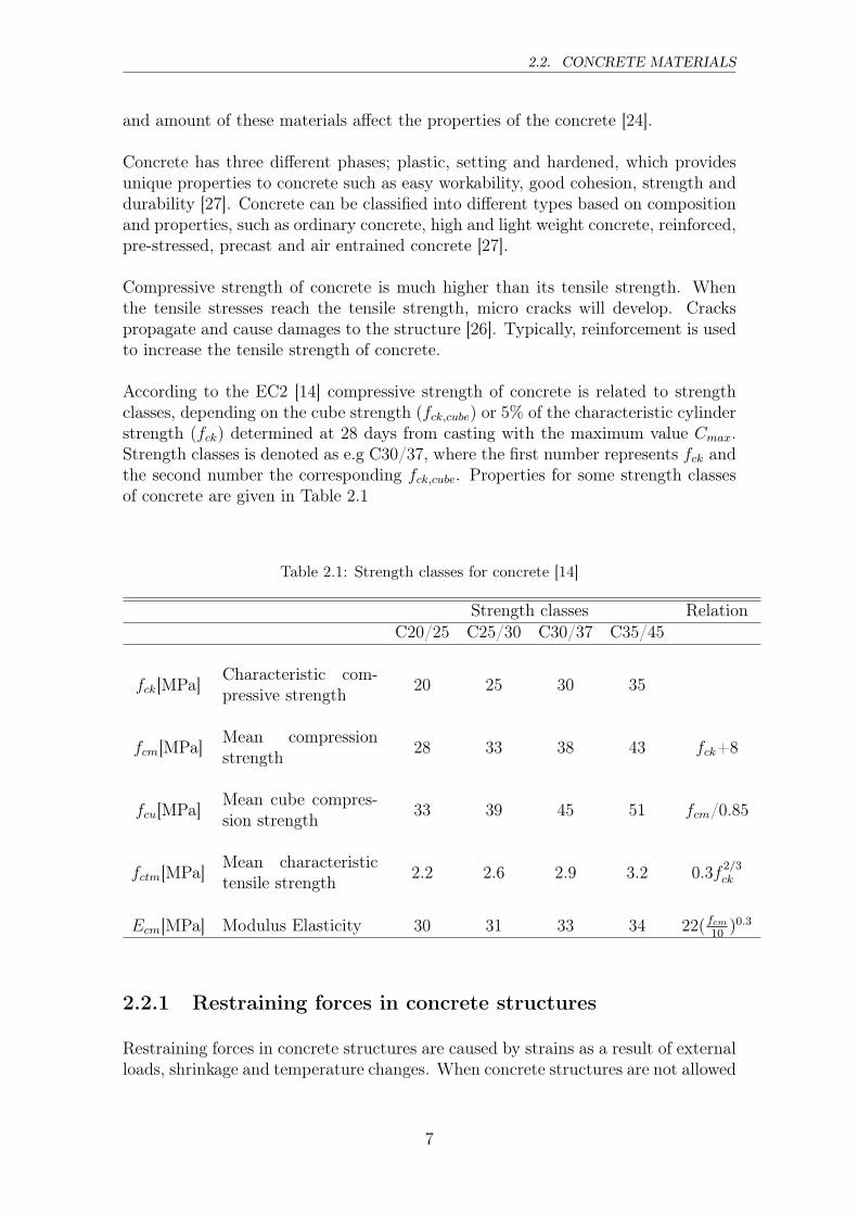
According to the EC2 [14] compressive strength of concrete is related to strengthclasses, depending on the cube strength (fck,cube) or 5% of the characteristic cylinderstrength (fck) determined at 28 days from casting with the maximum value Cmax.Strength classes is denoted as e.g C30/37, where the first number represents fck andthe second number the corresponding fck,cube. Properties for some strength classesof concrete are given in Table 2.1
Table 2.1: Strength classes for concrete [14]
Strength classes RelationC20/25 C25/30 C30/37 C35/45
fck[MPa] Characteristic com-pressive strength 20 25 30 35
fcm[MPa] Mean compressionstrength 28 33 38 43 fck+8
fcu[MPa] Mean cube compres-sion strength 33 39 45 51 fcm/0.85
fctm[MPa] Mean characteristictensile strength 2.2 2.6 2.9 3.2 0.3f 2/3
ck
Ecm[MPa] Modulus Elasticity 30 31 33 34 22(fcm10
)0.3
2.2.1 Restraining forces in concrete structures
Restraining forces in concrete structures are caused by strains as a result of externalloads, shrinkage and temperature changes. When concrete structures are not allowed
7
CHAPTER 2. THEORY, GUIDELINES AND STANDARDS
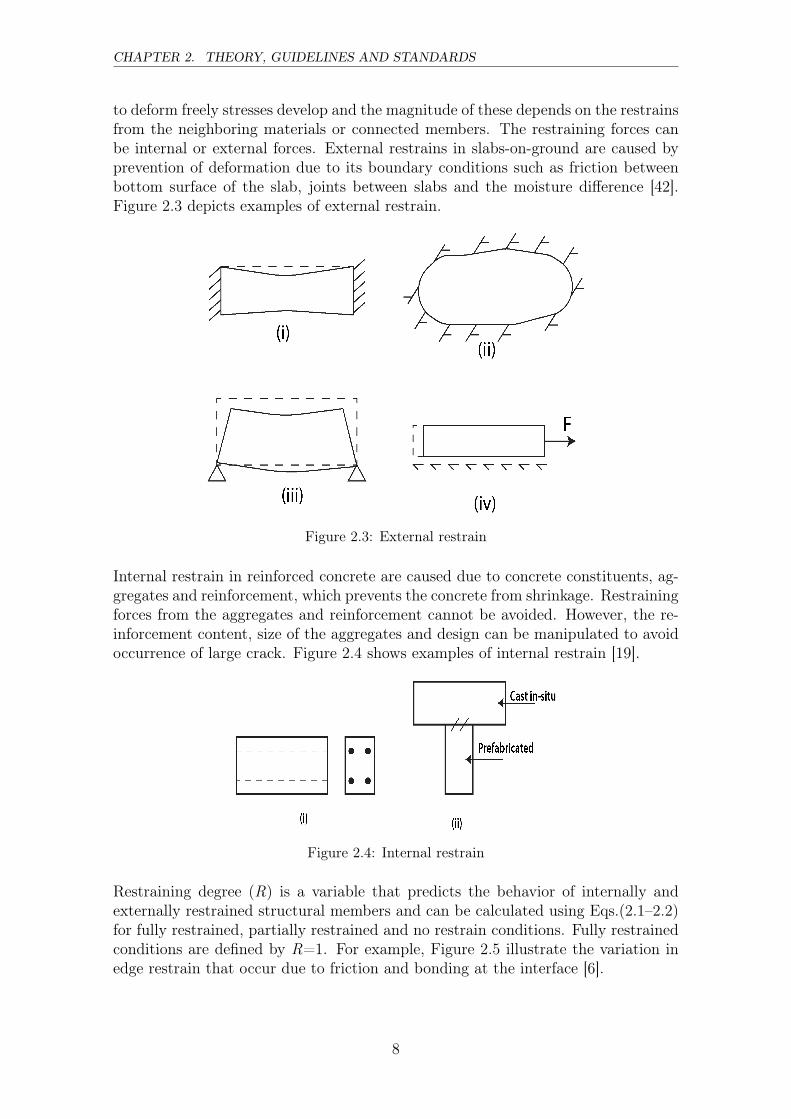
to deform freely stresses develop and the magnitude of these depends on the restrainsfrom the neighboring materials or connected members. The restraining forces canbe internal or external forces. External restrains in slabs-on-ground are caused byprevention of deformation due to its boundary conditions such as friction betweenbottom surface of the slab, joints between slabs and the moisture difference [42].Figure 2.3 depicts examples of external restrain.
Figure 2.3: External restrain
Internal restrain in reinforced concrete are caused due to concrete constituents, ag-gregates and reinforcement, which prevents the concrete from shrinkage. Restrainingforces from the aggregates and reinforcement cannot be avoided. However, the re-inforcement content, size of the aggregates and design can be manipulated to avoidoccurrence of large crack. Figure 2.4 shows examples of internal restrain [19].
Figure 2.4: Internal restrain
Restraining degree (R) is a variable that predicts the behavior of internally andexternally restrained structural members and can be calculated using Eqs.(2.1–2.2)for fully restrained, partially restrained and no restrain conditions. Fully restrainedconditions are defined by R=1. For example, Figure 2.5 illustrate the variation inedge restrain that occur due to friction and bonding at the interface [6].
8

2.2. CONCRETE MATERIALS
Restraint degree =Actual imposed strain
Imposed strain in case of full restrain(2.1)
R =εcεcT
(2.2)
R =σcEc
σc[1Ec
+ Ac
S.l]
(2.3)
where:S= total stiffness of the supports S = N/uN=normal forceu=total deflection of the supportAc=concrete areal=length of element
R =1
1 + [Ec
Es
Anet
As]
(2.4)
where: Anet=Ac-As
Figure 2.5: Variation in the degree of restrain [6]
2.2.2 Friction
Friction arises between two contact boundary surfaces due to opposing movements[25]. Frictional forces between a concrete slab and its sub-base arises as a results ofvolume changes in the slab due to shrinkage or temperature changes, which causeslocal movement of the slab against the sub-base from zero at the geometric centerof the slab, towards the maximum at the edge [16].
µ =maximum frictional force
normal force(2.5)
9

CHAPTER 2. THEORY, GUIDELINES AND STANDARDS
Figure 2.6: Friction behavior of slab-on-ground
When a slab-on-ground contracts due to shrinkage, the friction forces at the basewill develop stresses in the slab, which has a maximum at the slab center and zero atthe edges. As a result tensile stresses generated by the aggregates and reinforcementalso restrains the concrete [16]. A coefficient of friction is given by Eq.( 2.5), whichassume fully developed friction [6].
Coefficients of friction for different materials are shown in Table 2.3. In addition,when the slab is cast insitu against the sub-base consisting of for example sand andgravel, there will be an interface zone, where aggregates will be mixed with theconcrete creating a complex interfacial layer. Therefore, the friction along the slabwill be non-uniform [6]. To reduce the frictional restrain, moisture thermal effectsinsulating material are used.
Table 2.2: Coefficient of friction for a slab-on-ground
Material under slab-on-ground µCrushed aggregate – uncompacted and uneven ≥ 2Crushed aggregate – compacted and smooth 1
Sand layer – even 0.75Insulating material 0.5
2.3 Insulating polystyrene interface
Typically, slabs are placed on a sub-base, which acts as a capillary break layer.Usually, gravel, crushed aggregate and insulating layers is placed under the concrete
10

2.4. SHRINKAGE
slabs [37]. As mentioned above, shrinkage causes volume changes and consequentlyfriction between concrete slabs and the sub-base arises, this interlayer friction is oneof the factors that influence cracking [23]. There are different types of insulatingmaterials that can be used to avoid water penetration from the ground reachingthe concrete slabs and this can also reduce the friction between slabs and sub-base. Mineral wool, polyethylene and polystyrene materials are widely used as aninsulating material. There are two types of rigid polystyrene materials; expandedpolystyrene (EPS) and extruded polystyrene (XPS). Expanded polystyrene (EPS)is chemically stable, lightweight, moisture resistant and durable with no materialdecay. EPS has been used in construction for a long time as an insulating material[47]. An experimental study by Rantala et al. [28] showed a polystyrene layer hasapproximately 70 times higher water vapor resistance than mineral wool. EPS hasmore advantage over the XPS and is today widely used beneath concrete slabs onground as an insulating material.
2.4 Shrinkage
Shrinkage of concrete structural elements are common. Typically, concrete mix-tures contain more water than is required for the hydration. As concrete reach thehumidity equilibrium with its surrounding the excess water in the concrete is lostdue to evaporation or internal chemical reaction, the rate of which depends on thesurrounding temperature and humidity. As a result from shrinkage, the volume ofthe concrete decreases due to capillary tension [16]. Shrinkage of concrete take placein two stages: at early and later ages [36] as shown in the Figure 2.7.
Figure 2.7: Stages and types of shrinkage [36]
During the first 24 hours after casting, the concrete behave like a ductile material,shrinkage at this stage is more critical as the concrete has not gained strength. Asmall stress at this stage leads to larger shrinkage strain [19]. If the shrinkage isnot adequately controlled, it might lead to large movements and cause cracks. Incase of statically indeterminate structures, shrinkage will lead to the developmentof large stresses [19]. Free shrinkage is commonly used term shrinkage occurs whenthe relative humidity is less than 100%. Shrinkage caused under no restrain con-ditions will develop no stresses. The magnitude of the free, unrestrained shrinkagedepends on several factors such as temperature, relative humidity, concrete mixture
11

CHAPTER 2. THEORY, GUIDELINES AND STANDARDS
components, geometry and boundary conditions. Equation (2.6) is used to estimatethe shrinkage development over time [14].
εcs = γt.γRH .εcs0 (2.6)
where:εcs=free shrinkage strainεcs0=final free shrinkage strain of the materialγt=factor controlling the time of influenceγRH=factor to account for humidity of the surrounding humidity
Water content in the concrete is one of the main factors that affect shrinkage. Menzel[5] studied the relationship between water loss and shrinkage and showed that theinitial water in the capillaries is lost without contraction. Once the capillary waterevaporates and is adsorbed, shrinkage starts to occur as illustrated in Figure 2.8.
Shrinkage of concrete occur at two different stages and can be classified into dif-ferent types as show in Figure 2.7, such as plastic shrinkage, autogenous shrinkage,carbonation shrinkage and drying shrinkage.
Figure 2.8: Relationship between water loss and shrinkage [22]
2.4.1 Plastic shrinkage
In fresh concrete, water moves relatively freely, because of the density difference inthe concrete mixture. The water that is less dense moves upwards during compactionand this process is called bleeding [24]. As a result of evaporation water is lost fromthe surface and due to surface tension and capillary tension forces, the concretecontracts, which is know as plastic shrinkage. Due to plastic shrinkage the top
12

2.4. SHRINKAGE
surface of the concrete becomes harder in comparison with other portions of theconcrete and at this stage the concrete has low tensile strength, which results in theformation of plastic shrinkage cracking.
2.4.2 Autogenous shrinkage
Autogenous shrinkage occurs early and is attributed to chemical shrinkage and self-desiccation. The chemical shrinkage occurs due to reaction between the concretecomponents cement and water, defined by the C3S, C2S, C3A, and C4AF, throughchemical reactions [22] resulting in volume reduction, but no shrinkage strains. Asa result of chemical shrinkage void/pores will be generated leading to the beginningof autogenous shrinkage [43] as shown in Figure 2.9.
Figure 2.9: Shrinkage of high strength concrete with moisture exchange
In autogenous shrinkage water loss occurs from the void/pores as the hydration pro-cess that takes place in concrete mixture, without any loss of water to the exteriorsurrounding. Chemical shrinkage causes internal volume reduction, while autoge-nous shrinkage cause external volume reduction. Autogenous shrinkage happens inthree early stages, liquid phase, skeleton formation and hardening phase. As shownin Figure 2.9 the autogenous shrinkage is equal to the chemical shrinkage at theliquid phase, while chemical shrinkage stress is resisted in the skeletal formationphase due to stiffening of the concrete mix [22][43].
2.4.3 Carbonation shrinkage
Carbonation shrinkage occurs due to chemical reaction between cement constituent,water and carbon dioxide from the atmosphere during the hardening process ofthe concrete. The chemical reaction is shown below, where calcium hydroxide andcarbonic acid reacts to form calcium carbonate, while releasing water molecules,thereby reducing the pH of the concrete. In the case of reinforced concrete thereduction in pH causes corrosion of reinforcement bars [31]. Relative humidity of
13

CHAPTER 2. THEORY, GUIDELINES AND STANDARDS
the environment surrounding the concrete plays a vital role in the carbonation pro-cess. Comparatively, carbonation shrinkage and autogenous shrinkage are low withrespect to plastic and drying shrinkage [3].
H2CO2 + Ca(OH)2 → CaCO3 + 2H2O
2.4.4 Drying shrinkage
As the name indicates drying shrinkage can be defined as reduction in the concretevolume due to water loss during the drying process after hardening. During dryingshrinkage, water diffuse from the pores of the concrete to the surrounding environ-ment, and as a result of water movement and water loss from the capillary porestensile stresses are introduced in the concrete. By reinforcing the concrete the dry-ing shrinkage can be reduced by one-half [40]. There are several factors that affectsthe drying shrinkage, such as total volume of the aggregates used, size, grading andelastic properties of aggregates, water to cement content ratio, relative humidity,air quality, curing time and temperature. In normal strength concrete the dryingshrinkage is comparatively higher than in high strength concrete [41] as shown inFigure 2.10.
Figure 2.10: Shrinkage strain a) normal concrete and b) high strength concrete [41]
In case of slabs-on-ground after setting, non-linear gradient moisture will develop asa result of difference in relative humidity between bottom and top surfaces. Usually,the relative humidity will be much higher at the bottom compared to at the topsurface and this non-linear drying strain causes the top surface to shrink more thanthe bottom [41] as shown in Figure 2.11. Table 2.3 depicts the unrestrained dryingshrinkage for different concrete strength classes.
14

2.4. SHRINKAGE
Figure 2.11: Distribution of relative humidity and shrinkage strain in a slab
Table 2.3: Unrestrained drying shrinkage %� values for different classes of concreteaccording to Eurocode 2 [14]
.
Relative humidity(% )fck/fck,cube(MPa) 20 40 60 80 90 100
20/25 0.62 0.58 0.49 0.30 0.17 0.0040/50 0.48 0.46 0.38 0.24 0.13 0.0060/75 0.38 0.36 0.30 0.19 0.10 0.0080/95 0.30 0.28 0.24 0.15 0.80 0.0090/105 0.27 0.25 0.21 0.13 0.07 0.00
In accordance to EC2 [14] the shrinkage strain can be defined by
εcs = εcd + εca (2.7)
where:εcs is the total shrinkage strainεcd is the drying shrinkage strainεca is the autogenous shrinkage strain
According to EC2, autogenous and drying shrinkage can be calculated using thefollowing equations
εcd = βdskhεcd,0 (2.8)
where: kh is a coefficient depending on the notional size h0 according to Table 2.4.
Table 2.4: kh coefficient based on ho
h0 kh
100 1200 0.85300 0.75≥ 500 0.7
βds =(t− ts)
(t− ts) +√h30
(2.9)
15

CHAPTER 2. THEORY, GUIDELINES AND STANDARDS
where:t is the age of the concrete at the moment consideredts is the age of the concrete at the beginning of the drying shrinkage normally thisat the end of curlingh0 is the notional size (mm) of the cross section which is 2Ac/uAc is the concrete cross sectional areau perimeter of that part of the cross section which is exposed to drying
εca = βaskhεca(∞) (2.10)
where:
εca(∞) = 2.5(fck − 10)10−6 (2.11)
βas = 1− exp(−0.2t0.5) (2.12)
and with t given in days
2.5 Creep
For slabs-on-ground, deflection and curvature occurs as a result of shrinkage andcreep. Creep in concrete can be defined as the increase in strain due to sustainedstress that results in continued deformation [1]. These deformations mainly dependon the materials properties and time. When load is applied onto the concrete, thestress dependent deformation occurs [18]. As shown in Figure 2.12, initial deforma-tion occurs due to elastic strain and later due to creep strain that might reach itsfinal value after long time [1]. Increasing the rigidity of the aggregates can reducecreep.
Figure 2.12: Stress dependent strain of concrete at constant stress under loading [43]
Creep increases the strain capacity, since the tensile strength of the concrete isalmost independent prior to loading, thus creep is helpful for gradual applicationof tensile strain. Drying creep and basic creep are two different types of creep
16

2.6. CRACKING IN CONCRETE
[32]. Drying creep occurs due to moisture movement between specimen and theenvironment during the drying process and it also depends on the shape and size ofthe specimen. Basic creep occurs at constant moisture conditions and it does notdepend on the shape and size of the specimen. The effective modulus of elasticityfor concrete is calculated according to EC2 [14], Eq.( 2.13) for a load with a durationcausing creep.
1
Eeff(t,t0)=
1
Ecm+φ(t, t0)
Ec(28)(2.13)
where: Ec(28) = 1.05 Ecm(28), φ is the creep coefficient relevant for the load andtime interval.
2.6 Cracking in concrete
Usually, slabs-on-ground are sensitive to restrained drying shrinkage and cracks areformed as a results of higher induced stress than the tensile strength of the concrete,thus deteriorating the structures. Formation of cracks is a primary concern, whichplay a vital role for the response to compression and tension. Previously, it has beenshown that the stress-strain response of concrete is related to the formation of microcracks, which propagates between aggregates and surrounding mortar [1]. Figure2.13 illustrate the stress-strain curve for concrete loaded under uniaxial compression.
Figure 2.13: Stress-strain curve for concrete loaded with uniaxial compression [1]
The cracking process is illustrated in Figure 2.14. When the concrete start to crackthe stresses will be zero. Tension stress in the concrete will propagate a certain dis-tance, the transmission length So forming the crack, and other cracks can be formed
17

CHAPTER 2. THEORY, GUIDELINES AND STANDARDS
at different position away from the region +/- So, not affected by the initial crack.When several cracks are formed a new crack between these can be formed only whenthe distance is twice So [15] [6].
Figure 2.14: Mechanism of crack development in reinforced concrete under tension.a) Formation of first crack. b) When crack is stabilized [6]
The process of crack formation in reinforced concrete can be explained in threedifferent stages, un-cracked, cracking and stabilization of cracks as shown in Figure2.15. In the un-cracked stage the stresses developed will be less than the tensilestrength of the concrete. In Stage II, the stresses exceed the tensile strength resultingin the formation of cracks and as these propagate, a section analysis can be carriedout in the Stage II. There will be tensile stress between the cracks and un-crackedportions of concrete due to the transfer of forces, which makes the actual stiffnesshigher than the one assumed in the Stage II analysis and this phenomenon is calledtension stiffening [33].
Figure 2.15: Three cracking stages [33]
18

2.6. CRACKING IN CONCRETE
2.6.1 Curling
Curling or warping occurs in all types of slabs-on-ground. Causes for curling in slabsare due to differential strain from the difference in relative humidity between topand bottom. Hence the edges of the slab curl upward and loose contact with thesub-base, while it sinks at the center. As the moisture from the surface evaporatesfrom the surface of newly casted slabs, a differential moisture gradient is generated.Consequently, the differential shrinkage will cause the slab to bend/curl upwards[30] as shown in Figure 2.16.
There are several factors that influence the curling of slabs. Generally, upwardedge curling is caused due to negative moisture gradients and negative bending mo-ments, which causes compression at the bottom and tension at the top. Severalfactors such as high moisture content in the sub-base, concrete with high modulusof elasticity and slab surfaces exposed to dry air increases vertical deflection andmoisture gradients in the slab. Moreover, shrinkage gradients changes as a result ofrelative humidity as shown in Figure 2.17. Thus, concrete loses more water at lowrelative humidity, which cause the effect of shrinkage and due to shrinkage the slabbends upwards, which is known as curling or vertical deflection [40].
Figure 2.16: Curling of slab-on-ground
Figure 2.17: One year of shrinkage data for a 15-in thick slab as a function of relativehumidity with only top surface exposed to drying [40]
19

CHAPTER 2. THEORY, GUIDELINES AND STANDARDS
Several factors affects curling in addition to moisture gradient and total shrinkagesuch as aggregates, water-cement ratio and construction methods. Choosing theproper material can, as mentioned above, minimize curling. Also reinforcing theconcrete will largely reduce the curling effects [40]. Negative shrinkage results incurling of the upper half of slabs-on-grade and placing the reinforcement close tothe top will restrain the shrinkage. However, reinforcing the bottom half of theslabs further increase the upward curling as it add restrain at the bottom of theslab. Figure 2.18 shows the effect of reinforcement positions against curling [40].
Figure 2.18: Reinforcement position against curling [40]
2.6.2 Fracture energy
Figure 2.19 shows applied tensile stress against deformation for concrete in tension[34]. The applied stress reaches a maximum value equal to the tensile strength ofthe concrete, and as the tensile stress increase beyond this point cracks will formand the stresses will decreases as the cracks opens. When the stresses are at theirmaximum the crack width is zero, and when the stresses gradually becomes zero thedeformation is presented as a crack width. The area under the curve in Figure 2.19gives the fracture energy, defined as the energy required for crack formation per unitarea of crack plane [17].
The fracture energy of concrete GF is calculated according to the Model Code 1990[8], as
GF = GF0(fcmfcm0
)0.7 (2.14)
where: fcm0=10 MPa. GF0 is the base value of the fracture energy. it depends onthe maximum aggregate size dmax as given in Table 2.5
20

2.7. CRACK WIDTH ACCORDING TO EUROCODE 2
Figure 2.19: Strain-localization in a tensile specimen serving as model for fractureprocess zone. d) Possible effect of size on stress-strain diagram [30]
Table 2.5: Base value of fracture energy
dmax(mm) GF0(Nmm/mm2)
8 0.02516 0.03032 0.058
The fracture energy of concrete GF according to the Model Code 2010 [48] is givenby Eq.(2.15) and it can be seen that instead of aggregate size, compressive strengthof concrete is considered.
GF = 73fcm0.18 (2.15)
2.7 Crack width according to Eurocode 2
Minimum Reinforcement calculations
Cracking should be controlled in slabs-on-ground. The minimum reinforced re-quired for cracking control can be calculated according to EC2 [14] and is given byEq.(2.16). The amount of reinforcement is calculated by considering the equilibriumcondition between tensile forces in concrete and reinforcement.
As,minσs = kckfct,effAct (2.16)
21

CHAPTER 2. THEORY, GUIDELINES AND STANDARDS
where:As,min is the minimum area of the tensile reinforcementAct the area of the concrete in the tensile zonefct,eff effective tensile strength of the concretek coefficient of non uniform of self equilibrating stresseskc coefficient of the stress distribution in the cross section before cracking kc = 1 forrectangular cross section
Crack width calculations
As stated in the EC2 [14] to control the cracks the quasi-permanent load combinationshould be used. The crack width is calculated according to
Wk = Sr,max(εsm − εcm) (2.17)
where:Sr,max is the maximum crack spacingεsm is the mean strain in the reinforcementεcm is the mean strain concrete between cracks(εsm − εcm) can be calculated by using the equation
The differential strain between concrete and steel can be calculated as given by
(εsm − εcm) =σs − kt fct,effρct,eff
(1 + αeρp, eff)
Es≥ 0.6
σsEs
(2.18)
where:σs is the stress in the tension reinforcementαe is the ratio Es/Ecmρp,eff is the ratio As/Ac,effkt is the factor dependent on the duration of the loadAc,eff is the effective area of the concrete in tension
The maximum final crack spacing Sr,max can be calculated from
Sr,max = k3c+ k1k2k4φ/ρp,eff (2.19)
When the spacing of the bonded reinforcement exceeds 5(c+Φ/2) then the crackspacing is calculated using
Sr,max = 1, 3(h− x) (2.20)
where:φ is the diameter of the bar
22
2.8. CALCULATIONS OF CRACK WIDTH ACCORDING TO WIN-STATIK
c is the concrete coverk1 is a coefficient which takes of the bond properties of bonded reinforcementk2 is the coefficient which takes account of distribution of the strainh height of concrete sectionx distance from neutral axis to bottom of the slabThe coefficient k3 and k4 are given in the Swedish National Annex, k3 is 7 φ/c andk4 the EC2 recommended value is 0.425
2.8 Calculations of crack width according to WIN-statik
WIN-statik is a software program [50] that for designs problems and was here em-ployed to calculate the crack width according to the EC2 [14] design code for concretesection that requires reinforcement or check of specified reinforcement. The dimen-sioning of the required moment, axial force and shear force acting on the structurewere here considered for the limit states and the analysis performed on the crackedsection. Cracks and deformation can also be calculated based on the reinforcementcontent. It should be noted that WIN-statik is calculated, where non-linear is nottaken into consideration.
23

CHAPTER 2. THEORY, GUIDELINES AND STANDARDS
24

Chapter 3
Non-linear finite element analysis
3.1 Finite element analysis
The Finite Element Method (FEM) is a numerical method widely used in engineer-ing and technical fields as a numerical solution method for statical and dynamicalproblems. FEM can be defined as a general method for structural analysis, in whichthe geometric approximation involves replacement of continuous solids by combina-tions of a discrete number of structural elements, interconnect at a finite number ofnodal points [7],[11].
A mesh is defined as a particular arrangement of finite elements and is representednumerically by the algebraic equations required to be solved for unknowns at thenodes [7],[11]. The accuracy of the solution depends on the size and type of mesh,the finer the mesh size the higher the accuracy, which requires extensive computa-tional power. A fine mesh can be used when the stress gradient is expected to behigh [11]. In two-dimensional analysis triangular and rectangular meshes with threeand four nodes respectively, are commonly used due to that these are the simplestshapes for subdivision and boundary shape approximation. Although combinationof triangular and rectangular meshes is possible, it might not give the best results interms of accuracy. Moreover, triangular and rectangular meshes are not suitable forcomplex irregular geometric structures, where the elements will not fill the standardgeometry [11].
Generally, the stiffness matrix, which is related to the degrees of freedom, deter-mines the accuracy of the finite element analysis. For irregular geometric structuresisoparametric elements are used, with triangular or quadratic elements in which or-thogonality is not maintained between the sides of an element. Isoparametric (sameparameters) elements use auxiliary co-ordinates and the approximation points areequal to the number of nodes [13]. Usually, the solution is interpolated at nodes andbetween nodes through the use of shape functions. The advantages of using isopara-metric elements is that the approximation function are the actual shape function forthe element, which means that when the element sides are not having right angles,mapping functions are used to map those irregular elements into elements with regu-
25

CHAPTER 3. NON-LINEAR FINITE ELEMENT ANALYSIS
lar shapes and the integration is carried out for those regular shapes. Typically, theGauss numerical integration technique is used instead of exact integral calculationin order to reduce the required computation cost and to avoid the fraction quantitiesthat is difficult for exact integrals [13].
Figure 3.1: Finite element modeling steps based on [13]
In FE modeling, the first step is idealization in which the real structure is trans-formed to an analytical model and finally to a discrete FE model as shown Figure3.1. An FE model is created through the following typical steps:
i) Define the geometry of the structure
ii) Assign the property of the material with boundary conditions, such as load andsupports
iii) Discretize the model into elements.
iv) Perform final numerical approximation.
The general numerical solution procedure [9] is as follows:
Step 1
Assemble the structural stiffness matrix∑elem
[kloc] = [Kglob]
Step 2
Assemble the force vector ∑elem
{re} −→ {R}
Step 3
Impose boundary condition
26

3.2. NON-LINEAR ANALYSIS
Step 4
Solve[K]{D} = {R}
Step 5
Compute the internal forces at each element
˜{r} = [Ni Ti Mi Nj Tj Mj]T
{D} −→ {d}˜{r} = [k]{d}
where:kloc is the local stiffness matrixKglob is the global stiffness matrixre is element loadR is global loadd is local nodal deflectionD is global nodal deflection
3.2 Non-linear analysis
Typically, linear FEM model provides satisfactory approximations for several designcalculations. However, in reality most of the structure behavior is non-linear, for in-stance, the yielding of materials, local buckling, creep and crack opening and closing[9]. Nonlinearity in the structure can be classified as; 1) Material nonlinearity, wherethe material properties depends on the state of stress and strain (for e.g., materialyielding, crack and creep) 2) Contact nonlinearity, where contact areas changes withrespect to contact forces, for instance sliding contact with frictional forces, openingand closing of gaps between adjacent parts and 3) Geometric nonlinearity, wheredeformation cannot be neglected, consequently causing change in load direction asthey increase [9]. In these categories the problems are nonlinear due to stiffness,possible loads, and are functions of displacement or deformation. Therefore, theequation structural equilibrium [K ]{D}={R}, where [K ] is the coefficient stiffnessmatrix and {R} is the load vector, which becomes a function of the global nodaldeflection {D}. In order to determine {D}, an iterative process is required.
3.2.1 Iterative procedure
Analysis of non-linear material properties is not straightforward, since the deforma-tion is not equal to the size of the load. Therefore, the results can be realized byan iterative process where the Newton-Raphson (N-R) method is generally used for
27

CHAPTER 3. NON-LINEAR FINITE ELEMENT ANALYSIS
finding the roots of the polynomial equation. It was first described by Newton in1669, later Raphson generalized the procedure in 1690 [49] . Considering an examplewith a load (P) and displacement (u) curve as shown in Figure 3.2. At each node,summation of all the forces should result in zero, such that the structure will be inequilibrium. i.e., P-u=0
Figure 3.2: Non-linear load and deflection curve
Figure 3.3: (a) Newton-Raphson and (b) Modified Newton-Raphson iterations [9]
In a Newton-Raphson calculation for each load or deflection step, tangential stiffnesswill be computed and assembled at each iteration within each load step [9],[29]. Asshown in Figure 3.3(a), the initial load P1 is applied and the expect correspondingdisplacement is u1. The tangential stiffness (from the previous iteration for uA) Kt0
is used to extrapolate the displacement correction ua-u1. Equilibrium iteration re-duces the imbalance to reach zero [3]. Sequentially, increasing the small load step anditerating until convergence for each step provide correct solutions. The N-R methodis effective, however it will not always provide fast and reliable convergence. This isdue to that tangent stiffness needs to be calculated at each iteration, which increasethe computational expenses. It is not suitable for finding negative load increments
28

3.2. NON-LINEAR ANALYSIS
and also convergence fails when a large incremental load is applied. In the modifiedN-R method uses more iterations but the tangential stiffness Kt is not used for everyiteration, typically when a load increment is added as illustrated in Figure 3.3(b) [3].
The arc-length method can be used when the convergence analysis fails with theusing N-R method and for finding an equilibrium path beyond the critical path cap-turing negative load response behavior [9]. As shown in Figure 3.4 the arc-lengthfor both increment load and displacement is controlled during equilibrium itera-tions.Moreover, the turning points and limits can be passed using the arc-lengthmethod [9].
Figure 3.4: Arc-length iterations [3]
3.2.2 Fracture mechanics
Formation of crack and crack propagation is important for the performance of con-crete. Fracture mechanics provides fundamental rules under which cracks mightpropagate [21]. Fracture mechanics with a stress intensity approach considers astress field at the tip of the crack, which depends on the stress intensity factor Kgiven in Eq. (3.1), which depends on stresses and crack dimensions.
σ =K√2πr
(3.1)
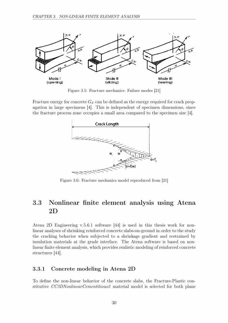
Cracks propagate when K reaches the critical value. Three mode of failure canoccur independently or in combination as shown in the Figure 3.5. Mode I: Openingmode, due to tensile. Mode II: Sliding, results due to in plane shear. Mode III:Tearing, occurs from out-of-plane shear.
In 1976 Hillerborg et al., [21] presented a model for fracture mechanics, in whichstresses are assumed to act at narrowly opened crack as shown in Figure 3.6. Thismodel was described only for Mode I, however, it can also be applied for Mode IIand III. In this model, when the concrete reaches its tensile strength the stress de-creases at the crack tip and when the crack opens the stress will decreases gradually.
29
CHAPTER 3. NON-LINEAR FINITE ELEMENT ANALYSIS
Figure 3.5: Fracture mechanics: Failure modes [21]
Fracture energy for concrete GF can be defined as the energy required for crack prop-agation in large specimens [4]. This is independent of specimen dimensions, sincethe fracture process zone occupies a small area compared to the specimen size [4].
Figure 3.6: Fracture mechanics model reproduced from [21]
3.3 Nonlinear finite element analysis using Atena2D
Atena 2D Engineering v.5.6.1 software [44] is used in this thesis work for non-linear analyses of shrinking reinforced concrete slabs-on-ground in order to the studythe cracking behavior when subjected to a shrinkage gradient and restrained byinsulation materials at the grade interface. The Atena software is based on non-linear finite element analysis, which provides realistic modeling of reinforced concretestructures [44].
3.3.1 Concrete modeling in Atena 2D
To define the non-linear behavior of the concrete slabs, the Fracture-Plastic con-stitutive CC3DNonlinearCementitious2 material model is selected for both plane
30

3.3. NONLINEAR FINITE ELEMENT ANALYSIS USING ATENA 2D
stress and plane strain idealization as shown in Figure 3.7. In plane stress problem,length of the slab is larger compare to its width and the stresses in the z directionwill be zero. In plane strain, the strain in the z direction will be zero and restricted,but there will be stresses.
Figure 3.7: Plane stress and plane strain idealization
This model is based on the smeared crack and crack band model, which combinesboth tensile and compressive behavior. It can be used for rotated or fixed crackapproaches based on Rankine failure criterion and can simulate concrete cracking[44]. In the crack band model as shown in Figure 3.8, fracture energy is consumedwithin the crack band.
Figure 3.8: Crack band model
31
CHAPTER 3. NON-LINEAR FINITE ELEMENT ANALYSIS
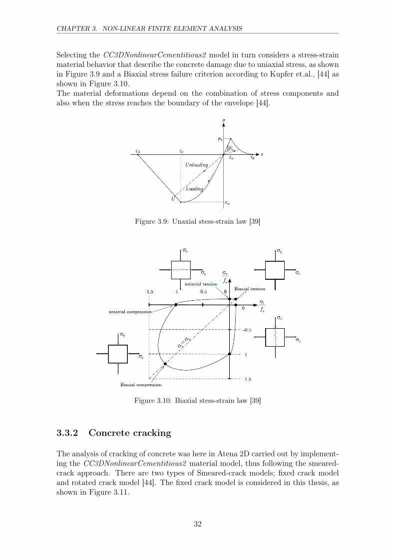
Selecting the CC3DNonlinearCementitious2 model in turn considers a stress-strainmaterial behavior that describe the concrete damage due to uniaxial stress, as shownin Figure 3.9 and a Biaxial stress failure criterion according to Kupfer et.al., [44] asshown in Figure 3.10.The material deformations depend on the combination of stress components andalso when the stress reaches the boundary of the envelope [44].
Figure 3.9: Unaxial stess-strain law [39]
Figure 3.10: Biaxial stess-strain law [39]
3.3.2 Concrete cracking
The analysis of cracking of concrete was here in Atena 2D carried out by implement-ing the CC3DNonlinearCementitious2 material model, thus following the smeared-crack approach. There are two types of Smeared-crack models; fixed crack modeland rotated crack model [44]. The fixed crack model is considered in this thesis, asshown in Figure 3.11.
32

3.3. NONLINEAR FINITE ELEMENT ANALYSIS USING ATENA 2D
Figure 3.11: Fixed crack model [44]
At the integration point, cracks will start to occur when the maximum principalstresses are equal to the tensile strength. Also, when the load is applied, the directionof the crack will not change, irrespective of the stress state changes [39]. Shear stresswill appear at the crack surface because of the change in direction of the crack andprincipal stress . Secondary cracks might occur at the same integration points whenthe stress direction changes orthogonally. In the rotated crack model the crackdirection rotates if the principal stress direction rotates during the loading [44], asshown in Figure 3.12.
Figure 3.12: Rotated crack model [44]
In Atena 2D with the CC3DNonlinearCementitious2 material model, for the shapestress-crack opening curve, the crack opening law derived by Hordijk [44] is employedfor normal concrete, see Eqs.(3.2 and 3.3).
σ
ft′ef = {1 + (c1
w
wc)3}exp(−c2
w
wc)(1 + c31)exp(−c2) (3.2)
wc = 5.14Gf
ft′ef (3.3)
33

CHAPTER 3. NON-LINEAR FINITE ELEMENT ANALYSIS
3.4 Reinforcement material model
In Atena 2D there are two options, discrete and smeared, for reinforcement model-ing. In smeared reinforcement modeling, the reinforcement is considered as a singlecomponent or as a part of the composite material [44]. In the discrete modeling,the reinforcement is model by truss element as reinforced bars. The present project,model discrete modeling of the reinforcement is used.
Properties for the reinforcement was defined in the Reinforcement material model,which consist of several types, linear; Bilinear, multi-linear and Bilinear with Hard-ening. In this work, Bilinear type was selected, which assume an elastic-perfectplastic bilinear stress-strain law of reinforcement as shown in Figure 3.13
Figure 3.13: Bilinear stress-strain curve for reinforcement [44]
The bond-slip model is one important part of the reinforcement bond model and inAtena 2D there are three different bond-slip models: CEB-FIB Model Code 1990 [8],user defined and slip law by Bigaj [44], which defines the bond strength relationshipbetween the reinforcement and surrounding concrete. The definition of a bond lawin Atena 2D is not based on the bond slip-bond stress but rather on bond slip-bondstrength [44], meaning that the slip will be zero until the bond strength is reached[12].
There are two options for the reinforcement bond; perfect connection and the bondmodel based on Bigaj work [44]. In this thesis, a bond model of connection type wasselected, which depends on the bond quality, and here the bond slip model accordingto the CEB-FIB Model Code 1990 [8] was used. There are several factors that affectthe bond stress-slip relationship, such as concrete strength, bar roughness, positionand orientation of bars, stress state and boundary conditions. Figure 3.14 illustratethe bond stress-slip curve.
τ = τmax(s/s1)2 for 0 ≤ s ≤ s1 (3.4)
34

3.4. REINFORCEMENT MATERIAL MODEL
Figure 3.14: Bond stress-slip relation (monotonic loading) [44]
τ = τmax for s1 < s ≤ s2 (3.5)
τ = τmax − (τmax − τf )(s− s2s3 − s2
) for s2 < s ≤ s3 (3.6)
τ = τf for s3 < s (3.7)
The initial curve part in Figure 3.14 illustrates the stage where ribs enter into themortar matrix, which is characterized by micro cracking and local crushing. In thenext stage is the horizontal level that occurs for confined concrete where crushingand shearing of the concrete between the ribs occurs, while the last stage representsthe decrease in bond strength as a result of reduction in the bond resistance causedby splitting cracks along the bar [8].
Equations (3.4-3.7) are used to calculate the bond stress between concrete and re-inforcing steel. Table 3.1 shows the parameters for ribbed reinforcement providedby international standards [8], which depends on the concrete strength and bondcondition.
Table 3.1: Parameter for the bond stress calculation [48]
Unconfined concrete Confined concreteGood bond All other bond Good bond All other bond
s1 0.6 mm 0.6 mm 1.0 mm 1.0 mms2 0.6 mm 0.6 mm 3.0 mm 3.0 mms3 1.0 mm 2.5 mm Clear rib spacing Clear rib spacingα 0.4 0.4 0.4 0.4τmax 2.0
√f ck 1.0
√f ck 2.5
√f ck 1.25
√f ck
τf 0.15τmax 0.15τmax 0.4τmax 0.4τmax
35

CHAPTER 3. NON-LINEAR FINITE ELEMENT ANALYSIS
3.5 Interface material
In this work the EPS, sand and gravel are considered as interface materials. Aninterface material model is used to simulate the contact between concrete slab andsoil sub-base. The interface material settings are based on a Mohr-Coulomb crite-rion with tension cut off. It should be noted that in Atena 2D, if the input valuefor the tensile strength, friction coefficient and cohesion is all zero this will createcomputational problem [44]. Figure 3.15 shows the failure surface for an interfaceelement.
Figure 3.15: Failure surface of interface element [44]
To define the interface material behavior, the following input parameters are neces-sary: tensile strength (ft) normal stiffness (Knn), tangential stiffness (Ktt), cohesion(c) and friction coefficient (µ). There are few recommendations in the manual forAtena 2D [11], but the following is documented: i) Usually, the friction coefficientwill not be less than 0.1, except for special conditions such as oiled surfaces, andtherefore 0.3-0.5 will here be a better estimate. ii) The cohesion value should begreater than or equal to the interface tensile strength and the friction coefficient.iii) When the interface properties are unknown, it is recommended to set the inter-face value to 0.25 or 0.5 of the tensile strength for the weaker material next to theinterface. For the initial stiffness it is 10 times the adjacent finite elements as givenby Eq.(3.8).
Knn & Ktt =Ecmle
10 (3.8)
Where:Knn=normal stiffnessKtt=tangential stiffnessEcm=modulus of elasticityle=element size
36

3.6. SUB-BASE MATERIAL PROPERTY
3.6 Sub-base material property
In this work soil and gravel are used as the sub-base material in 3D Drucker-Pragerplasticity. Properties of soil and sub-base material are defined in the material prop-erty including modulus of elasticity, Poisson′s ratio and Drucker-Prager criterionparameters [10]. The model for Drucker-Prager plasticity is based on the generalplasticity model [44] and the yielding surface can be defined by Eq. (3.9).
F pDP (σy) = αI1 +
√J2 − k = 0 (3.9)
The material constant friction angle (φ) and the cohesion (c) are the most commonlyused parameters estimated by the Mohr-Coulomb model. There is a direct relationbetween these parameters and also the shape defining parameter (α) and failuresurface parameter k of the Drucker-Prager model, see Eqs. (3.11-3.10). The plasticpotential can be defined by Eq.(3.12).
α =2sinφ√
3(3− sinφ)(3.10)
k =6 c cosφ√3(3− sinφ)
(3.11)
Gp(σij) = β1√3I1 +
√2J2 (3.12)
Here β determines the return direction. When material is compacted during crushingthis becomes β < 0, when the material volume is preserved it is β = 0 and if β> 0the material is dilating. A predictor-corrector algorithm, as shown in Figure 3.16,is used for the plastic model and the return mapping algorithm is considered as theplastic flow is not perpendicular to the failure surface [44].
3.7 Boundary conditions and loads
Settings up proper boundary conditions are necessary for accurate FEM analyses[44]. A half-symmetrical model is set up for the FEM analysis in this thesis. Atthe symmetry line, support conditions for both slab and sub-base were consideredto be fixed in the x-direction and free in the y-direction. At the bottom of sub-base, a fixed end support condition was applied for both the x- and y -directions.Furthermore, the slab is subjected to the non-restrained condition, which meansthat it is free at the slab edge. Three different load types were considered for theanalysis, self-weight of slab, applied external load and gradient shrinkage load. Loadsare gradually applied step-by-step in Atena 2D and the crack width was measured atthe maximum element nodes [44]. Self-weight of the slab is calculated automatically
37

CHAPTER 3. NON-LINEAR FINITE ELEMENT ANALYSIS
Figure 3.16: Plastic predictor corrector algorithm [44]
by the program considering the dimensions of the slab; with the direction of the self-weight considered being in the vertical downward direction. In Atena 2D shrinkageis applied as initial strain (Eps) i.e., a constant volume reduction for the wholestructure, and its behavior is modeled as a load effect.
f(x, y) = (K +Kx · x+Ky · y) · Eps (3.13)
Macro element shrinkage is selected in Atena 2D and the input data for the shrinkagefield is given in the Eq.(3.13) are entered. The gradient shrinkage load was calculatedaccording to the WSP user guide [46]. The Figure 3.17 shows the shrinkage gradientapplied considering the relative humidity of 100% at the bottom and 55% at the topof the slab and the alpha value was set to 0.2 for different concrete strength classesand thickness of the slab. A uniformly distributed load is considered as the externalapplied load on the surface of the slab.
Figure 3.17: Gradient shrinkage [46]
38

Chapter 4
Numerical Examples
4.1 Modeling approach
Non-linear finite element analysis was performed using Atena 2D to determine theeffects from shrinkage loads on slabs-on-ground to predict the non-linear behaviourof cracks and vertical deflection of the slabs. Furthermore, a parametric study ispresented in this chapter. The simulations were carried out to demonstrate theaccuracy of the model and to predominantly identify the crucial parameters. Thefollowing steps were carried out in the numerical simulations:
1. Pre-processing stage: The geometry, material data, boundary condition andloading are defined in Atena 2D and these parameters were varied to run theanalysis for different models.
2. Analysis stage: Atena 2D runs the analysis solver for the different models andresults are extracted at the element nodes.
3. Post-processing stage: In this stage, the results from the solver are plotted inform of graphs and evaluated.
The numerical examples consist of the following studied cases:
• Convergence study: performed to optimize the mesh size and numerical finiteelement model with respect to crack width, deformation and crack pattern
• Parametric study: investigation of crack width with respect to varying slabdimension, concrete strength class, reinforcement content, varying bar diam-eter, bond definition, fracture energy, varying sub-base, the frictional effectsbetween the slab and sub-base, effect of external load, and bar diameter.Furthermore, parametric studies were performed according to WSP guide in-puts [46]
39

CHAPTER 4. NUMERICAL EXAMPLES
• The crack widths obtained from numerical simulation with Atena 2D werecompared with the corresponding from WIN-statik in which the internal forcesobtained from Atena 2D is used as an input to calculate the crack widths. ForWIN-statik the moment and axial forces were calculated based on the Eqs.(4.1and 4.2) to find the crack widths. Furthermore, theoretical calculation of frac-ture energy according to Model Codes 1990 [8] and 2010 [48] were performed.
F = fctm · b · h(1 + α
2) (4.1)
M = fctm · w(1− α
2) (4.2)
Where: w=bh2/6
The geometry of the model is as shown below, with the boundary conditions sym-bolically marked. In this chapter, different parameters were varied to study theresponse of slabs-on-ground, maximum crack width and vertical deflection was usedas a measure of the response. A cut-off was set for minimum visible crack widthat 0.01 mm. Maximum crack widths were extracted at the element nodes and plot-ted against increasing shrinkage load. Maximum vertical deflection values for slabsare graphically presented with a magnification scale of 20 and obtained data wereplotted against increasing shrinkage load.
Figure 4.1: Geometry of the model
4.2 Convergence analysis
The convergence analyses were performed as basic evaluation for the finite elementmodels in order to obtain the optimal mesh size in the numerical model. In themodel, an isoparametric quadrilateral element type was chosen and different meshsizes of 30 mm, 40 mm, 60 mm and 80 mm were tested, with all other parameterskept constant. A gradient shrinkage load was applied and a convergence analysiswas performed for the maximum crack width and vertical deflection. The slab andsand as sub-base were modeled by using interface elements between them and theanalyses were carried out for self-weight and shrinkage load of the slab. Longitudinalreinforcement of bar diameter Φ=10 mm and reinforcement content ρ=0.3% wereconsidered. Convergence analyses were performed for both plane stress and planestrain idealizations. For plane stress conditions, plane stress was considered for slab
40

4.2. CONVERGENCE ANALYSIS
and plane strain for the sub-base. In the plane strain condition both the slab andsub-base were analyzed under plane strain assumptions.
For the concrete material, the CC3DNonlinCementitious2 model was chosen inAtena 2D [12]. For the reinforcement, a bilinear material model was chosen to-gether discrete bar elements and for the sub-base, the sand properties are taken intoconsideration and modeled with the Drucker-Prager plasticity parameters. Eachload step was performed for 100 iterations. Dead weight of the slab were analyzedwith 10 load step to achieve 100% with a load multiplier of 0.1, whereas the shrinkageload were analyzed for 100 load steps with a load multiplier of 0.02. The crackingpattern, vertical deflection and the maximum crack width for every 10 loads step atthe element nodes were analyzed. The properties of the materials are shown in thetables.
Table 4.1: Concrete material model parameter for strength class C30/37 mean values
Properties unit value
Elastic modulus GPa Ecm = 33Poissons ratio ν = 0.2Coefficient of thermal expansion 1/K α = 1.2 · 10−5
Tensile strength MPa fctm = 2.9Compressive strength MPa fcm = 38Fracture energy MN/m GF = 7.5 · 10−5
Table 4.2: Reinforcement model, bi-linear reinforcement
Properties unit value
Elastic modulus GPa Es = 200Specific material weight MN/m3 γs = 7.85 · 10−2
Coefficient of thermal expansion 1/K α = 1.2 · 10−5
Yeild strength MPa fy = 500
41

CHAPTER 4. NUMERICAL EXAMPLES
Table 4.3: Sub-base model, mean values Drucker-Prager plasticity
Properties unit value
Elastic modulus MPa Esand = 20Poissons ratio ν = 0.3Tensile strength MPa ft = 0.001Compressive strength MPa fc = 1Coefficient of thermal expansion 1/K α = 1.2 · 10−5
Specific material weight MN/m3 γs = 1.8 · 10−2
Angle of friction Radians φ = 0.524Drucker-Prager criterion parameter MN/m3 α = 0.231Drucker-Prager parameter MPa k = 0.001
Table 4.4: Interface element properties
Properties unit value
Normal stiffness GN/m3 Knn = 8500Tangential stiffness GN/m3 Ktt = 8500Tensile strength MPa ft = 5 · 10−4
Cohesion MPa ft = 0Friction coefficient µ = 0.75
4.2.1 Plane stress
The crack width response to the applied shrinkage load for varying mesh sizes theplane stress condition is illustrated in Figure 4.2. The maximum crack widths areextracted from the element nodes. As shown in Figure 4.2 for all the element sizetested the results were converging. At finer element sizes the maximum crack widthdecreased, which is in agreement with that finer mesh sizes gives more accurateresults, as discussed earlier in section 3.1. However, finer element sizes requiresexcessive CPU time and therefore a 30 mm mesh size was excluded from the studyin favor of 40 mm mesh that was chosen for the subsequent analyses, motivated bythat the results for 30 mm and 40 mm elements gives similar results. The relativeconvergence errors obtained are less than 10 % as shown by the convergence.
42

4.2. CONVERGENCE ANALYSIS
As shown in Figure 4.3 the maximum vertical deflection tend to increase for thefiner mesh sizes, as shown by the maximum vertical deflection. According to theobtained results and experienced gained during the study, the element mesh size 40mm and isoparametric quadrilaterals were incorporated for the further numericalanalyses. Crack pattern and vertical deflection for varying element size is depictedin Figure 4.4.
0 0.1 0.2 0.3 0.4 0.5 0.6 0.7 0.8 0.9 10
0.2
0.4
0.6
Shrinkage load (per mille)
Maxcrack
width
(mm
)
3 cm4 cm6 cm8 cm
Figure 4.2: Convergence study for maximum crack for the plane stress model fordifferent element sizes
0 0.1 0.2 0.3 0.4 0.5 0.6 0.7 0.8 0.9 102468
101214
Shrinkage load (per mille)
Verticaldeflection
(mm
)
3 cm4 cm6 cm8 cm
Figure 4.3: Convergence study for vertical deflection for the plane stress model fordifferent element sizes, measured at the edge of the slab
43

CHAPTER 4. NUMERICAL EXAMPLES
Element size 30 mm
Element size 40 mm
Element size 60 mm
Element size 80 mm
Figure 4.4: Crack pattern for different mesh sizes in plane stress model
4.2.2 Plane strain
Maximum crack width response from applied shrinkage load for varying mesh size inthe plane strain idealization is shown in Figure 4.5. Maximum crack width increasedfor the finer mesh sizes. The load-vertical deflection graph for the plane strain con-dition with varying element size is illustrated in Figure 4.6. The maximum verticaldeflection converges for 30 mm, 40 mm and 60 mm mesh size as depicted in Figure4.6 but not for the 80 mm.
Maximum vertical deflection decreases for 40 mm mesh size at a shrinkage loadof 0.9 %� and for 60 mm at 0.8%� because here the maximum crack width is reachedchanges to the other position and therefore a jump in the curve is observed andthe crack width then starts growing at this position, as explained in the section2.6. Crack pattern and vertical deflection for varying element sizes are depictedin Figure 4.7. For the parametric study, only plane stress was considered becausethe maximum crack width is almost constant when the element size was varied, asshown in Figure 4.8, while in the plane strain condition the maximum crack widthchanges when the elements size is varied.
44

4.3. MODEL CHECK AND ANALYSIS METHOD
0 0.1 0.2 0.3 0.4 0.5 0.6 0.7 0.8 0.9 10
0.2
0.4
0.6
0.8
1
1.2
1.4
1.6
Shrinkage load (per mille)
Maxcrack
width
(mm
)3 cm4 cm6 cm8 cm
Figure 4.5: Convergence study for maximum crack for the plane strain model fordifferent element sizes
0 0.1 0.2 0.3 0.4 0.5 0.6 0.7 0.8 0.9 10
2
4
6
8
10
12
14
Shrinkage load (per mille)
Verticaldeflection
(mm
)
3 cm4 cm6 cm8 cm
Figure 4.6: Convergence study for maximum crack for the plane strain model fordifferent element sizes
4.3 Model check and analysis method
4.3.1 Model check
In this project, all the studies were performed with a half-symmetry model, sincethe full model consume large CPU-time and increase the post processing times.As a first step, a half-symmetry model was compared with a full symmetry modelto verify the output for maximum crack widths as seen in Figure 4.9 and verticaldeflection as in Figure 4.10 for both the models. The maximum crack width andvertical deflection shown in Figure 4.9 were similar for both models. Therefore, thehalf-symmetry model could be chosen for further parametric studies. Crack patternand deflection for both half symmetry and full models are shown in Figure 4.11. Asshown in Figure 4.12 the results shows good correlation. The moment line drawnat the bottom of the slab integrates the stress over the cross section of the slab.
45

CHAPTER 4. NUMERICAL EXAMPLES
Element size 30 mm
Element size 40 mm
Element size 60 mm
Element size 80 mm
Figure 4.7: Crack patterns for different mesh sizes in plane strain model
2 3 4 5 6 7 80
0.5
1
1.5
Element size (cm)
Maxcrack
width
(mm
)
Plane stressPlane strain
Figure 4.8: Maximum crack width comparision of plane strain model and plane stressassumptions for different element sizes
The position of the moment line does not change the moment and axial forcesover the cross section. Maximum moment causes the maximum crack width andthe stress will gradually decrease to zero. The maximum moment and axial forcesobtained were used as input for the WIN-statik program to check the crack widthsobtained in Atena 2D. Inputs for the model is given in Table 4.5.
46

4.3. MODEL CHECK AND ANALYSIS METHOD
Table 4.5: Inputs for the symmtery and full model
Concrete class C30/37Tensile reinforcement 4Φ10Bond type GoodLength of slab 8 mThickness of slab 0.2 mFriction at interface 0.75Sub-base Sand
0 0.1 0.2 0.3 0.4 0.5 0.6 0.7 0.8 0.9 10
0.1
0.2
0.3
Shrinkage load (per mille)
Maxcrack
width
(mm
)
4 m symmetry model8 m full model
Figure 4.9: Comparision of crack width for half symmetry and full model.
0 0.1 0.2 0.3 0.4 0.5 0.6 0.7 0.8 0.9 10
2
4
6
8
10
12
14
Shrinkage load (per mille)
Verticaldeflection
(mm
)
4 m symmetry model8 m full model
Figure 4.10: Load-vertical deflection response to shrinkage load
47

CHAPTER 4. NUMERICAL EXAMPLES
Half symmetry model slab, with length 4 m (mirrored after analysis)
Full model slab length 8 m
Figure 4.11: Comparision of vertical deflection and crack patterns for half symmetrymodel and full model
0 1 2 3 4 5 6 7 8 9 100
0.1
0.2
0.3
0.4
0.5
Length of slab (m)
Maxcrack
width
(mm
)
AtenaWIN-statik
Figure 4.12: Relationship of crack width for half length symmetric model and fulllength model
4.3.2 Analysis method
A simply supported slab of 5 m was analyzed in Atena 2D and this is a stati-cally determinate structure, where reactions and internal forces are calculated usingequilibrium equations. A uniformly distributed load 10 kN/m2 was applied on thesimply supported slab. The maximum bending moment was calculated using Eq.(4.3). The cracked and deformed slab is shown in Figure 4.13, where the cracks wereobserved at the bottom of the slab due to tension.
M =qL2
8(4.3)
Typically, slabs-on-ground are placed on an infinite medium, which provides contin-uous support for the concrete slab considered as an indeterminate structure, sincethe slab is extra constrained by the supporting sub-base and have higher stiffness.Moment and axial forces were calculated using the numerical software Atena 2D toavoid the complexity of theoretical calculations. Crack widths obtained for both the
48

4.4. PARAMETRIC STUDY
Figure 4.13: Crack patterns for the statically detereminate structure
statically determinate and indeterminate structures were listed in Table A.3 (SeeAppendix). The crack pattern are shown in Figure 4.14.
Figure 4.14: Crack pattern for the statically indetereminate structure
4.4 Parametric study
Parametric studies were performed to analyze the effects of key parameters on thecrack formation in the slabs-on-ground model, restrained at the sub-base and sub-jected to gradient shrinkage. Key parameters such as reinforcement content, con-crete strength class, bond slip definition, fracture energy, varying slab dimensions,bar diameter, applied external load, varying friction coefficient for different sub-basematerials were analyzed.
The Table shows the list of different parameter studied in this project and thebold values in the table shows reference model values 4.6 Furthermore, parametricstudies were performed based on WSP guide inputs [46].
Table 4.6: Parameters used in this study
Length 5, 10, 15 and 20 mHeight 150, 200, 250 and 300 mmConcrete strength class C20/25, C30/37 and C35/37Varying sub-base Sand and GravelInterface material Sand, Gravel and EPSBond Type Poor, Good and PerfectExternal load 10kN/m2
Reinforcement content 0.2, 0.3, 0.4 and 0.5%
49

CHAPTER 4. NUMERICAL EXAMPLES
4.4.1 Varying slab length
Structural dimensions of the slabs influence the crack behavior. Maximum crackresponse curves and vertical deflection for varying slab lengths are presented in Fig-ures 4.15 and 4.16, while other parameter are kept constant as shown in Table 4.7.As indicated in Figure 4.15, the slab length influence the development of cracks. At5 m length there was no crack observed, but as the slab length increased to 10 m thefirst crack appeared for a shrinkage load of 0.3 %� and for slabs of length 15 and 20m the first crack appeared at 0.4 %� shrinkage load. As the shrinkage load increasedthe maximum crack width also increased non-linearly, while the maximum verticaldeflection value varies linearly for increasing shrinkage as shown in Figure 4.16. Thecrack pattern and vertical deflection for varying lengths are shown in Figure 4.17.Maximum moment obtained from the Atena 2D is used as an input for WIN-statikand the crack width was calculated and plotted as illustrated in Figure 4.18 whichshows similar crack width pattern.
Table 4.7: Input for the slab varying length
Concrete class C30/37Tensile reinforcement 4Φ10Bond type GoodLength of slab 5,10,15 and 20 mThickness of slab 0.2 mFriction at interface 0.75Sub-base Sand
0 0.1 0.2 0.3 0.4 0.5 0.6 0.7 0.8 0.9 10
0.1
0.2
0.3
0.4
Shrinkage load (per mille)
Maxcrack
width
(mm
)
20 m15 m10 m5 m
Figure 4.15: Crack response curve for varying lengths
50

4.4. PARAMETRIC STUDY
0 0.1 0.2 0.3 0.4 0.5 0.6 0.7 0.8 0.9 10
2
4
6
8
10
12
14
Shrinkage load (per mille)
Verticaldeflection
(mm
)20 m15 m10 m5 m
Figure 4.16: Deflection of slab for varying lengths subjected to shrinkage load
Slab length 5 m
Slab length 10 m
Slab length 14 m
Slab length 20 m
Figure 4.17: Crack patterns and vertical deflection for different slab lengths
4.4.2 Varying slab thickness
The thickness of the slab varied from 150 mm to 200 mm, 250 mm and 300 mm,while other parameter were kept constant as listed in the Table 4.8. The maximumcrack width response was measured as a result of shrinkage load. Thickness hasgreat influence on the maximum crack width development with respect to appliedshrinkage load as shown in Figure 4.19. Although, first crack developed for the 200mm, 250 mm and 300 mm slab thickness, the maximum crack width was seen forthe 300 mm slab and the lowest crack width was obtained for the 150 mm thickslab. It is evident from Figure 4.20 that the smaller the slab thickness the smallerthe maximum calculated vertical deflection. Vertical deflection was higher as theslab thickness was increased as illustrated in Figure 4.20. Crack pattern and vertical
51

CHAPTER 4. NUMERICAL EXAMPLES
0 5 10 15 200
0.2
0.4
Length of slab (m)
Maxcrack
width
(mm
)AtenaWIN-Statik
Figure 4.18: Relationship between varying slab length and corresponding maximumcrack width
deflection is depicted in Figure 4.21. Maximum moment obtained from the Atena2D was also here used as an input for WIN-statik and the crack width was calculatedand plotted as illustrated in Figure 4.22.
Table 4.8: Input for the different concrete quality
Concrete class C30/37Tensile reinforcement 4Φ10Bond type GoodLength of slab 10 mThickness of slab 0.15, 0.20, 0.25 and 0.30 mFriction at interface 0.75Sub-base Sand
0 0.1 0.2 0.3 0.4 0.5 0.6 0.7 0.8 0.9 10
0.1
0.2
0.3
0.4
0.5
Shrinkage load (per mille)
Maxcrack
width
(mm
)
150 mm200 mm250 mm300 mm
Figure 4.19: Varying slab thickness and crack width for applied shrinkage load
52

4.4. PARAMETRIC STUDY
0 0.1 0.2 0.3 0.4 0.5 0.6 0.7 0.8 0.9 10
4
8
12
16
20
24
Shrinkage load (per mille)
Verticaldeflection
(mm
)150 mm200 mm250 mm300 mm
Figure 4.20: Load-vertical deflection of slab for varying thickness when subjected toshrinkage load
Thickness 150 mm slab
Thickness 200 mm slab
Thickness 250 mm slab
Thickness 300 mm slab
Figure 4.21: Crack pattern for slab with varying thickness
4.4.3 Concrete strength class
Slabs with different concrete strength classes were investigated for varying shrinkageload by considering the mean values as listed in Table 2.1 and the parameters listedin Table 4.9. Different concrete strength classes tested shows similar maximum crackwidth response for the applied shrinkage loads as seen in Figure 4.23. Maximumcrack width for concrete class C35/45 is relatively wider than for the other concretestrength classes. For both class C25/30 and C20/25 similar crack widths are shownand the load response have a tendency to reach plateaus for increased shrinkage.For each concrete strength classes the crack width response curve is non-linear asshown in Figure 4.23.
53
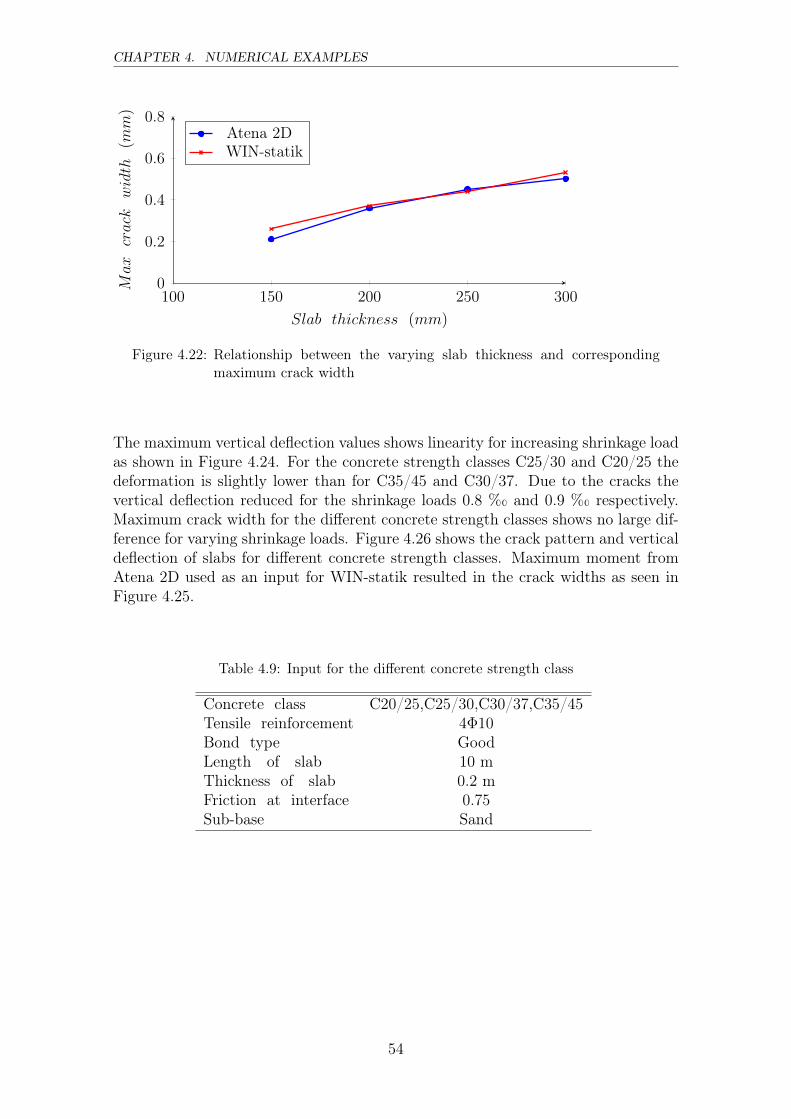
CHAPTER 4. NUMERICAL EXAMPLES
100 150 200 250 3000
0.2
0.4
0.6
0.8
Slab thickness (mm)
Maxcrack
width
(mm
)Atena 2DWIN-statik
Figure 4.22: Relationship between the varying slab thickness and correspondingmaximum crack width
The maximum vertical deflection values shows linearity for increasing shrinkage loadas shown in Figure 4.24. For the concrete strength classes C25/30 and C20/25 thedeformation is slightly lower than for C35/45 and C30/37. Due to the cracks thevertical deflection reduced for the shrinkage loads 0.8 %� and 0.9 %� respectively.Maximum crack width for the different concrete strength classes shows no large dif-ference for varying shrinkage loads. Figure 4.26 shows the crack pattern and verticaldeflection of slabs for different concrete strength classes. Maximum moment fromAtena 2D used as an input for WIN-statik resulted in the crack widths as seen inFigure 4.25.
Table 4.9: Input for the different concrete strength class
Concrete class C20/25,C25/30,C30/37,C35/45Tensile reinforcement 4Φ10Bond type GoodLength of slab 10 mThickness of slab 0.2 mFriction at interface 0.75Sub-base Sand
54

4.4. PARAMETRIC STUDY
0 0.1 0.2 0.3 0.4 0.5 0.6 0.7 0.8 0.9 10
0.1
0.2
0.3
0.4
0.5
Shrinkage load (per mille)
Maxcrack
width
(mm
)C35/45C30/37C25/30C20/25
Figure 4.23: Load-crack response for different concrete strength classes
0 0.1 0.2 0.3 0.4 0.5 0.6 0.7 0.8 0.9 10
2
4
6
8
10
12
14
Shrinkage load (per mille)
Verticaldeflection
(mm
)
35/4530/3725/3020/25
Figure 4.24: Vertical deflection-load response for different concrete strength classes
C35/45 C30/37 C25/30 C20/250
0.2
0.4
0.6
0.8
1
Concrete strength classes
Maxcrack
width
(mm
)
AtenaWIN-statik
Figure 4.25: Relationship between varying concrete strength classes and correspond-ing maximum crack width
55

CHAPTER 4. NUMERICAL EXAMPLES
C20/25
C25/30
C30/37
C35/45
Figure 4.26: Crack patterns and vertical deflection for difference concrete strengthclasses
4.4.4 Reinforcement content
Reinforcement content is one key parameter to control the crack formation and ver-tical deflection caused by shrinkage loads. Reinforcement content is varied throughthe number of bars for both top and bottom of the slab, keeping the concrete coverconstant to 50 mm on either side. The bar diameter was kept constant, all otherparameters are listed in Table 4.10.
Increase in the reinforcement content reduces the maximum crack width. No changeswere observed in crack width for 0.5 and 0.4 % reinforcement content. However,for 0.2 % reinforcement, the maximum crack width increased with varying appliedshrinkage load as shown in Figure 4.27.
The vertical deflection was linear for increase in the shrinkage load and co-relatedwith varying reinforcement contents as seen in Figure 4.28. After reaching certainshrinkage load steps, vertical deflection slightly reduces with higher reinforcementpercentage. Crack pattern and vertical deflection for different reinforcement con-tent on the application of shrinkage load is shown in Figure 4.29. The maximummoment obtained from Atena 2D used as an input for WIN-statik gave the crackwidth plotted in Figure 4.30.
56

4.4. PARAMETRIC STUDY
Table 4.10: Input for the different reinforcement content
Concrete class C30/37Tensile reinforcement 0.5, 0.4, 0.3 and 0.2 %Bond type GoodLength of slab 10 mThickness of slab 0.2 mFriction at interface 0.75Sub-base Sand
0 0.1 0.2 0.3 0.4 0.5 0.6 0.7 0.8 0.9 10
0.2
0.4
0.6
0.8
1
1.2
1.4
Shrinkage load (per mille)
Maxcrack
width
(mm
)
0.5%0.4%0.3%0.2%
Figure 4.27: Change in reinforcement content on crack-width
0 0.1 0.2 0.3 0.4 0.5 0.6 0.7 0.8 0.9 10
2
4
6
8
10
12
14
Shrinkage load (per mille)
Verticaldeflection
(mm
)
0.5%0.4%0.3%0.2%
Figure 4.28: Vertical deflection as reinforcement content is varied
57

CHAPTER 4. NUMERICAL EXAMPLES
Reinforcement content 0.2%
Reinforcement content 0.3%
Reinforcement content 0.4%
Reinforcement content 0.5%
Figure 4.29: Crack pattern for different reinforcement contents
0 0.1 0.2 0.3 0.4 0.5 0.6 0.70
0.4
0.8
1.2
1.6
2
Reinforcement content (%)
Crack
width
(mm
) AtenaWIN-statik
Figure 4.30: Relationship between varying reinforcement content and correspondingmaximum crack width
To complement the reinforcement results the maximum tensile stresses were ob-tained. The reinforcement stress values leaps out at shrinkage load 0.6 %� showingless prominent stress at high reinforcement contents as depicted in Figure 4.31
58

4.4. PARAMETRIC STUDY
0 0.1 0.2 0.3 0.4 0.5 0.6 0.7 0.8 0.9 10
50
100
150
200
250
300
Shrinkage load (per mille)
Reinforcementstress
(MPa) 0.50%
0.40%0.30%0.20%
Figure 4.31: Reinforcement stress
4.4.5 Bond definition
Bond between concrete and reinforcement is important factor that influence the cal-culation of the crack width. Crack widths are plotted for shrinkage load for differentqualities of bond with all other parameters held constant, as listed in Table 4.11.As shown in Figure 4.32 the first crack appears at the same shrinkage load for allthree types of bonding poor, good and perfect bond. However the correspondingcrack width increases for poor bond and good bond respectively, and the dominatingcracks appear at similar shrinkage load steps. For perfect bond the maximum crackwidth plateaued as the shrinkage load was increased. Vertical deflection of the slabswere similar in all type of bonding tested as shown in Figure 4.33. Crack patternand vertical deflection for the different bond type are depicted in Figure 4.34. Themaximum moment obtained from Atena 2D as an input for WIN-statik gave thecrack width and plotted in Figure 4.35.
Table 4.11: Input for different concrete qualities
Concrete class C30/37Tensile reinforcement 4Φ10Bond type poor, good and perfectLength of slab 10 mThickness of slab 0.2 mFriction at interface 0.75Sub-base Sand
59

CHAPTER 4. NUMERICAL EXAMPLES
0 0.1 0.2 0.3 0.4 0.5 0.6 0.7 0.8 0.9 10
0.1
0.2
0.3
0.4
0.5
Shrinkage load (per mille)
Maxcrack
width
(mm
)poor bondgood bondperfect bond
Figure 4.32: Crack width for different type of reinforcement bond
0 0.1 0.2 0.3 0.4 0.5 0.6 0.7 0.8 0.9 10
2
4
6
8
10
12
14
Shrinkage load (per mille)
Verticaldeflection
(mm
)
Poor bondGood bondPerfect bond
Figure 4.33: Vertical deflection of slab for different bond types
Poor bond
Good bond
Perfect bond
Figure 4.34: Crack patterns for different bond types
60

4.4. PARAMETRIC STUDY
poor good perfect0
0.1
0.2
0.3
0.4
0.5
0.6
0.7
0.8Maxcrack
width
(mm
)Atena
WIN-statik
Figure 4.35: Relationship between varying bond and corresponding maximum crackwidth
4.4.6 Fracture energy
Fracture energy is a key parameter for crack propagation and can be defined ac-cording to Model Code 1990 [14] and 2010 [48] respectively, which depends on theaggregate size. According to Model Code 2010 [48] the minimum aggregate size of8 mm was considered, since larger aggregates reduces compressive strength of theconcrete with negligible effects on the tensile strength. And all other parameter arelisted in Table 4.12. In Figure 4.36 the effect of fracture energy GF=0.065 kN/m forModel Code 1990 and GF=0.1405 kN/m for Model Code 2010 is illustrated. Themaximum crack width was slightly higher for the Model Code 1990 compared toModel Code 2010 [8]. Vertical deflection with the two different fracture energies ex-hibits linear values for increasing shrinkage load as shown in Figure 4.37. In Figure4.38 crack pattern and vertical deflection from the fracture energy is presented. Themaximum moment from Atena 2D as an input for WIN-statik gave crack widthsplotted in Figure 4.39.
Table 4.12: Input for different fracture energies
Concrete class C30/37Tensile reinforcement 4Φ10Fracture Energy MC 1990 and MC 2010Bond type GoodLength of slab 10 mThickness of slab 0.2 mFriction at interface 0.75Sub-base Sand
61
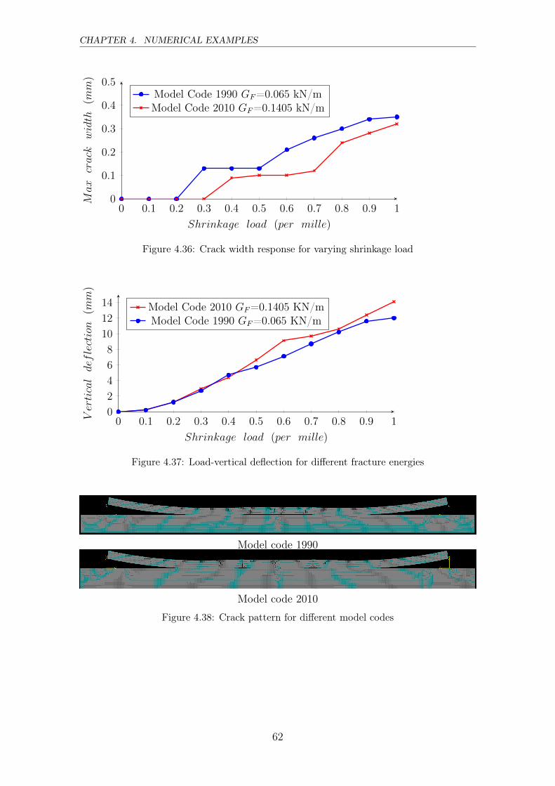
CHAPTER 4. NUMERICAL EXAMPLES
0 0.1 0.2 0.3 0.4 0.5 0.6 0.7 0.8 0.9 10
0.1
0.2
0.3
0.4
0.5
Shrinkage load (per mille)
Maxcrack
width
(mm
)Model Code 1990 GF=0.065 kN/mModel Code 2010 GF=0.1405 kN/m
Figure 4.36: Crack width response for varying shrinkage load
0 0.1 0.2 0.3 0.4 0.5 0.6 0.7 0.8 0.9 10
2
4
6
8
10
12
14
Shrinkage load (per mille)
Verticaldeflection
(mm
)
Model Code 2010 GF=0.1405 KN/mModel Code 1990 GF=0.065 KN/m
Figure 4.37: Load-vertical deflection for different fracture energies
Model code 1990
Model code 2010
Figure 4.38: Crack pattern for different model codes
62

4.4. PARAMETRIC STUDY
MC 1990 MC 20100
0.1
0.2
0.3
0.4
0.5
0.6
0.7
0.8Maxcrack
width
(mm
)Atena
WIN-statik
Figure 4.39: Relationship between fracture energies and corresponding maximumcrack width
4.4.7 Varying sub-base
For slabs-on-ground, the sub-base is one of the important factors. Here, sand andgravel are used as a sub-base, while the interface material are varied and all otherparameters kept constant, see Table 4.13. Sand, gravel and EPS with a frictioncoefficient (µ) of 0.75, 1 and 0.5, respectively, are used to determine the crack widthresponse to varying shrinkage loads. There was no differences observed between thethree interface materials with respect to the maximum crack width and all threefollow similar pattern as shown in Figure 4.40. In Figure 4.41 the load-deflectionas a result of varying load for different interface materials is presented. The load-deflection curve increases for increasing shrinkage load for all three interfaces tested.Crack pattern and vertical deflection is depicted in Figure 4.42. The maximum mo-ment from Atena 2D as an input for WIN-statik gave the crack width plotted inFigure 4.43.
Table 4.13: Input parameters
Concrete class C30/37Tensile reinforcement 4Φ10Friction co-efficient at interface 0.5, 0.75 and 1Bond type GoodLength of slab 10 mThickness of slab 0.2 mFriction at interface 0.75Sub-base Sand
63

CHAPTER 4. NUMERICAL EXAMPLES
0 0.1 0.2 0.3 0.4 0.5 0.6 0.7 0.8 0.9 10
0.1
0.2
0.3
0.4
0.5
Shrinkage load (per mille)
Maxcrack
width
(mm
)µ=0.75µ=1µ=0.5
Figure 4.40: Crack width and shrinkage load for varying interface material
0 0.1 0.2 0.3 0.4 0.5 0.6 0.7 0.8 0.9 10
2
4
6
8
10
12
14
Shrinkage load (per mille)
Verticaldeflection
(mm
)
µ=0.75µ=1µ=0.5
Figure 4.41: Vertical deflection curve for different interface materials
Interface fricition coefficient 0.75
Interface fricition coefficient 1
Interface fricition coefficient 0.5
Figure 4.42: Crack patterns for sand as sub-base and varying interface coefficient
64

4.4. PARAMETRIC STUDY
0 0.25 0.5 0.75 10
0.3
0.6
Coefficient of fricition (µ)
Maxcrack
width
(mm
)Atena
WIN-statik
Figure 4.43: Relationship between varying sub-base and corresponding maximumcrack width
Gravel is used as sub-base material, the interface material varied while all otherparameters were kept constant as listed in Table 4.14. Slightly higher crack widthwas observed in combination with gravel as sub-base and EPS as interface mate-rial, as shown in Figure 4.44. Vertical deflection for gravel as sub-base is shownin Figure 4.45, with results similar to sand as sub-base, therefore no large changeswere observed for sand and gravel as sub-base. In Figure 4.50 crack pattern andvertical deflection is indicated for gravel as sub-base with varying friction coefficient.
Table 4.14: Input parameters
Concrete class C30/37Tensile reinforcement 4Φ10Friction co-efficient at interface 0.5, 0.75 and 1Bond type GoodLength of slab 10 mThickness of slab 0.2 mFriction at interface 0.75Sub-base Gravel
65

CHAPTER 4. NUMERICAL EXAMPLES
Table 4.15: Sub-base model, mean values for gravel Drucker-Prager Plasticity
Properties unit value
Elastic modulus MPa EGravel = 40Poissons ratio ν = 0.3Tensile strength MPa ft = 0.0025Compressive strength MPa fc = 1.5Coefficient of thermal expansion 1/K αt = 1.2 · 10−5
Specific material weight MN/m3 γs = 20 · 10−2
Angle of friction Radians φ = 0.698Drucker-Prager criterion parameter MN/m3 α = 0.315Drucker-Prager parameter MPa k = 0.003
0 0.1 0.2 0.3 0.4 0.5 0.6 0.7 0.8 0.9 10
0.1
0.2
0.3
0.4
0.5
Shrinkage load (per mille)
Maxcrack
width
(mm
)
µ=0.75µ=1µ=0.5
Figure 4.44: Varying crack width for different interfaces with gravel as sub-base
0 0.1 0.2 0.3 0.4 0.5 0.6 0.7 0.8 0.9 10
2
4
6
8
10
12
14
Shrinkage load (per mille)
Verticaldeflection
(mm
)
µ=0.75µ=1µ=0.5
Figure 4.45: Load-vertical deflection for different interface materials
66

4.4. PARAMETRIC STUDY
Interface fricition coefficient 0.75
Interface fricition coefficient 1
Interface fricition coefficient 0.5
Figure 4.46: Crack patterns for gravel as sub-base and varying interface coefficient
0 0.25 0.5 0.75 10
0.3
0.6
Coefficient of fricition (µ)
Maxcrack
width
(mm
)
AtenaWIN-statik
Figure 4.47: Relationship between varying sub-base and corresponding maximumcrack width
4.4.8 Effect of external load with different sub-base
Slabs-on-ground with sand and gravel as sub-base was tested for applied externaluniformly distributed load and no external load conditions with sand as interfacematerial in both the cases. Parameters for the analysis is given in Table . The 10kN/m2 load was applied as external load together with the shrinkage load, givingmaximum crack width response as shown in the Figure 4.48. When no load wasapplied there was no change in crack width behavior for both the sub-bases of sandand gravel respectively. However, the crack width behavior was different for the twoexternally loaded cases had larger crack widths compared with no load conditions,while gravel with external load showed much higher crack widths. In Figure 4.49the load-vertical deflection curve for external load and no external load condition ispresented. Linear deflections for increasing shrinkage load were observed for bothcases, while the vertical deflections with loads applied were much lower than for thenon-loaded conditions.
67

CHAPTER 4. NUMERICAL EXAMPLES
Crack pattern and vertical deflection as a results of load and no load conditionsare shown in Figure 4.50. In WIN-statik program maximum moment from Atena2D used as an inputs to find the crack widths and plotted as shown in the Figure 4.51.
Table 4.16: Input for load conditions
Concrete class C30/37Tensile reinforcement 4Φ10External load 10 kN/m2
Bond type GoodLength of slab 10 mThickness of slab 0.2 mFriction at interface 0.75Sub-base Sand & Gravel
0 0.1 0.2 0.3 0.4 0.5 0.6 0.7 0.8 0.9 10
0.2
0.4
0.6
0.8
1
Shrinkage load per mille
Maxcrack
width
(mm
)
Sand no external loadGravel no external loadSand with external loadGravel with external load
Figure 4.48: Crack width for applied load and no load conditions
0 0.1 0.2 0.3 0.4 0.5 0.6 0.7 0.8 0.9 10
2
4
6
8
10
12
14
16
Shrinkage load (per mille)
Verticaldeflection
(mm
)
sand no external loadgravel no external loadsand with external loadgravel with external load
Figure 4.49: Load-vertical deflection for applied load and no external load
68

4.5. PARAMETERS ACCORDING TO WSP GUIDE INPUTS
Sand with no external load
Gravel with no external load
Sand with external load
Gravel with external load
Figure 4.50: Crack pattern for sand and gravel as sub-base with or without externalload
Sand gravel sand(EL) gravel(EL)0
0.2
0.4
0.6
0.8
Maxcrack
width
(mm
)
AtenaWIN-statik
Figure 4.51: Relationship between varying sub-base and corresponding maximumcrack width
4.5 Parameters according to WSP guide inputs
According to recommendations in the WSP guide [49] parameters are varied to checkthe effect on the crack width and vertical deflection. In this analysis the minimumamount of reinforcement considered are according to EC2 [14] for controlled crackingand the concrete cover was set to be 30 mm on the top and 50 mm on the bottomof the slab.
69
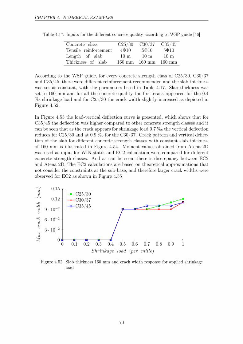
CHAPTER 4. NUMERICAL EXAMPLES
Table 4.17: Inputs for the different concrete quality according to WSP guide [46]
Concrete class C25/30 C30/37 C35/45Tensile reinforcement 4Φ10 5Φ10 5Φ10Length of slab 10 m 10 m 10 mThickness of slab 160 mm 160 mm 160 mm
According to the WSP guide, for every concrete strength class of C25/30, C30/37and C35/45, there were different reinforcement recommended and the slab thicknesswas set as constant, with the parameters listed in Table 4.17. Slab thickness wasset to 160 mm and for all the concrete quality the first crack appeared for the 0.4%� shrinkage load and for C25/30 the crack width slightly increased as depicted inFigure 4.52.
In Figure 4.53 the load-vertical deflection curve is presented, which shows that forC35/45 the deflection was higher compared to other concrete strength classes and itcan be seen that as the crack appears for shrinkage load 0.7 %� the vertical deflectionreduces for C25/30 and at 0.9 %� for the C30/37. Crack pattern and vertical deflec-tion of the slab for different concrete strength classes with constant slab thicknessof 160 mm is illustrated in Figure 4.54. Moment values obtained from Atena 2Dwas used as input for WIN-statik and EC2 calculation were compared for differentconcrete strength classes. And as can be seen, there is discrepancy between EC2and Atena 2D. The EC2 calculations are based on theoretical approximations thatnot consider the constraints at the sub-base, and therefore larger crack widths wereobserved for EC2 as shown in Figure 4.55
0 0.1 0.2 0.3 0.4 0.5 0.6 0.7 0.8 0.9 10
3 · 10−2
6 · 10−2
9 · 10−2
0.12
0.15
Shrinkage load (per mille)
Maxcrack
width
(mm
)
C25/30C30/37C35/45
Figure 4.52: Slab thickness 160 mm and crack width response for applied shrinkageload
70

4.5. PARAMETERS ACCORDING TO WSP GUIDE INPUTS
0 0.1 0.2 0.3 0.4 0.5 0.6 0.7 0.8 0.9 10
2
4
6
8
10
12
14
16
Shrinkage load (per mille)
Verticaldeflection
(mm
)C25/30C30/37C35/45
Figure 4.53: Vertical deflection of slab for varying concrete strength classes whensubjected to shrinkage load
C25/30
C30/37
C35/45
Figure 4.54: Crack pattern for slabs of different concrete strength classes with slabthickness 160 mm
For the slab thickness 200 mm the parameters listed in Table 4.18 was used. Slabthickness was set to 200 mm and for all the concrete strength classes, the first crackwas appeared for the 0.2 %� shrinkage load and for C25/30 the crack width slightlyincreased with shrinkage load 0.7 %� as depicted in Figure 4.56.
In Figure 4.57 the load-vertical deflection curve is presented, which shows thatfor C35/45 the deflection was slightly higher compared to other concrete strengthclasses. Crack pattern and deformation of slab for different concrete strength classeswith a constant slab thickness of 200 mm is illustrated in Figure 4.58. Moment val-ues obtained from Atena 2D was used as input for WIN-statik and EC2 calculationswere compared for different concrete strength class. And also here, there is discrep-ancy between EC2 and Atena. Larger crack width were observed for EC2 as shownin Figure 4.59
71

CHAPTER 4. NUMERICAL EXAMPLES
Figure 4.55: Relationship between Atena, WIN-statik(Atena) and WIN-statik(Analytical) calculations for different concrete strength classes
Table 4.18: Input for the different concrete strength classes according to the WSPguide [46]
Concrete class C25/30 C30/37 C35/45Tensile reinforcement 5Φ10 6Φ10 6Φ10Length of slab 10 m 10 m 10 mThickness of slab 200 mm 200 mm 200 mm
0 0.1 0.2 0.3 0.4 0.5 0.6 0.7 0.8 0.9 10
5 · 10−2
0.1
0.15
0.2
Shrinkage load (per mille)
Maxcrack
width
(mm
)
C25/30C30/37C35/45
Figure 4.56: Slab thickness 200 mm and crack width response for applied shrinkageload
72

4.5. PARAMETERS ACCORDING TO WSP GUIDE INPUTS
0 0.1 0.2 0.3 0.4 0.5 0.6 0.7 0.8 0.9 10
2
4
6
8
10
12
14
16
Shrinkage load (per mille)
Verticaldeflection
(mm
)C25/30C30/37C35/45
Figure 4.57: Vertical deflection of slab for varying concrete strength classes whensubjected to shrinkage load
C25/30
C30/37
C35/45
Figure 4.58: Crack pattern for slabs of different concrete strength classes with slabthickness 200 mm
For the slab thickness 300 mm the parameters listed in Table 4.19 was used. Slabthickness was set to 300 mm and for all the concrete strength classes the first crackappeared for the 0.2 %� shrinkage load and for all the concrete quality the crackwidth response curve for varying shrinkage load is very much similar as shown inFigure 4.60.
In Figure 4.61 the load-vertical deflection curve is presented, which shows thatfor C35/45 the deflection was slightly higher compared to other concrete strengthclasses. Crack pattern and deformation of slab for different concrete strength classeswith a constant slab thickness of 300 mm is illustrated in Figure 4.62. Moment val-ues obtained from Atena 2D was used as input for WIN-statik and EC2 calculationswere compared for different concrete strength classes as shown in Figure 4.63
73

CHAPTER 4. NUMERICAL EXAMPLES
Figure 4.59: Relationship between Atena, WIN-statik(Atena) and WIN-statik(Analytical) calculations for different concrete strength classes
Table 4.19: Inputs for the different concrete quality according to WSP guide [46]
Concrete class C25/30 C30/37 C35/45Tensile reinforcement 5Φ12 6Φ12 7Φ12Length of slab 10 m 10 m 10 mThickness of slab 300 mm 300 mm 300 mm
0 0.1 0.2 0.3 0.4 0.5 0.6 0.7 0.8 0.9 10
5 · 10−2
0.1
0.15
0.2
Shrinkage load (per mille)
Maxcrack
width
(mm
)
C25/30C30/37C35/45
Figure 4.60: Slab thickness 300 mm and crack width response curve for appliedshrinkage load
74

4.5. PARAMETERS ACCORDING TO WSP GUIDE INPUTS
0 0.1 0.2 0.3 0.4 0.5 0.6 0.7 0.8 0.9 102468
1012141618
Shrinkage load (per mille)
Verticaldeflection
(mm
)C25/30C30/37C35/45
Figure 4.61: Vertical deflection of slab for varying concrete strength classes whensubjected to shrinkage load
C25/30
C30/37
C35/45
Figure 4.62: Crack pattern for slabs of different concrete strength classes with slabthickness 300 mm
For the WSP recommended values the comparison between Atena 2D and WIN-statik analysis, smaller crack widths were obtained in Atena 2D than WIN-statikbecause Atena 2D consider the softening of concrete around the cracks, while EC2gives 0.3 to 0.4 mm larger crack widths as shown in Figures 4.55, 4.59 and 4.63.And, EC2 considers only the statistically determinant problem and the calculatedcrack widths are generally overestimated. Also, for calculating the crack widths forstatistically indeterminate structure the use of EC2 should be avoided, but it willbe on the safe side.
75

CHAPTER 4. NUMERICAL EXAMPLES
Figure 4.63: Relationship between Atena, WIN-statik(Atena) and WIN-statik(Analytical) calculations for different concrete strength classes
76

Chapter 5
Discussion
Cracks on slabs-on-ground occurs due to gradient shrinkage and is here analyzedwith the non-linear finite element analysis, using Atena 2D. Cracks develop whenthe stress in the concrete becomes larger than its tensile strength. Cracks can bedeveloped either on top or on the bottom surface of the slab. Cracks at the bottomsurface might be interesting with respect to durability, however these cracks are notvisible. Therefore, the cracks at the top surface provide more information whendesigning for the key parameters to avoid crack formation and to increase the dura-bility, functionality and aesthetics. EC2 is used as a basis for calculation of the crackwidth, but it considers only the vertical load and a rectangular stress distributionassumed in the compression zone. However, numerical modeling will facilitate thesimulation and visibility of cracks across the entire dimension of slabs subjected tovarious types of loads and also considers the constraints from the sub-base.
The first step in the numerical model is the convergence analysis. In this project,convergence analysis was done for two different idealizations, i.e. plane stress andplane strain, to determine the optimum element size for both conditions. For theplane stress condition only the slab is considered as under plane stress because thelength of the slab is larger than its width, so that the slab behave like a beam andthe stress in the z-direction will be zero. However, the sub-base was not modeledunder plane stress conditions because it will allow lateral expansion in the thirddirection due to non zero poissons ratio resulting in larger vertical displacementcompared with plane strain. In the plane strain idealization, both slab and sub-baseare considered to be under plane strain, assuming both as infinite media. Typically,the plane strain model is suitable for the relatively large or infinite media, where thestress in the third direction is considered, while strains and deflection are negligible.The maximum crack width and vertical deflections of the slab is assumed to be afunction of shrinkage load, as were considered for the convergence test. The resultpresented in Figures 4.2, 4.3, 4.5 and 4.6 shows satisfactory convergence for both theidealizations. As explained earlier in section 3.1, finer mesh sizes gives better theresults and for further analysis an element size of 4 cm was selected, which providedsatisfactory results.
77

CHAPTER 5. DISCUSSION
A parametric study was performed using the crack width and deflection as a func-tion of the gradient shrinkage load. Firstly, the slab length and thickness werevaried and the load-deflection response and maximum crack width measured. Asshown in Figure 4.13 the length of the slab does not have considerable effect onthe maximum crack width. Reflecting on the empirical formula presented in EC2it can be seen that the maximum width of the crack is independent of its length.This study shows similar results. It is obvious that by increasing the length of theslab its stiffness decreases. Based on linear mechanics stiffer the element lesser thedisplacement. However the results depicted in Figure 4.14 indicates approximatelythe same amount of vertical deflection for almost all the models except for the 5 mslab. The behavior of the response curve is due to the non-linear behavior of theslab, which occurs after propagation of the crack in the slab. In other words, whenthe crack becomes wide enough the slab enters into the stage of nonlinearity.
As shown in Figure 5.1 the maximum crack width for 20 m slab length starts atthe top surface, grows till the middle of the slab and then become wider, while theconcrete stresses at the top becomes zero. Apparently, wider cracks are not seenon the top due to that the high stress in the tensile reinforcement holds the crackstogether at the top. Also there are horizontal cracks opening in the bottom of theslab, which are called splitting cracks. Also diagonal cracks were observed, which area type of shearing crack. Reduction in the load bearing capacity induces diagonalshear crack before ultimate load. These cracks are caused by the decrease in bondstrength as a result of reduction in bond resistance caused by splitting cracks alongthe bar as explained more in section 3.4.
Figure 5.1: Maximum crack width detailing
Due to the shrinkage load, the negative moment results in that the top of the slab isunder tension while the bottom is under compression as shown in Figure 5.2. Whenthe length of the slab is reduced to 5 m there was no visible maximum crack width.This is because of the constraint between slab and sub-base that was not enough todevelop cracks for the smaller length of the slab as shown in Figure 4.15.
The maximum crack width achieved by numerical analysis for all models approxi-mately fits the amount of maximum crack width prescribed by EC2 (See Appendix).Also, at maximum crack width, it should be noted that maximum stress occurs inthe tensile reinforcement.
78

Figure 5.2: Maximum stress in the slab
The gradient shrinkage alpha 0.2 was applied as shown in Figure 3.17, and after theanalysis, the ratio of maximum reinforcement stress at the bottom and top calculatedat the maximum crack width showed accurate stresses in the reinforcement as shownin Figure 5.3, with results due to the applied shrinkage gradient as calculated below.
Maximum Tensile stress in the top reinforcement= 296 MPaMaximum Compressive stress in the bottom reinforcement= 71 MPaThe ratio of maximum reinforcement stress =71/296= 0.2
Therefore, Atena 2D provides a good indication of crack widths and deflection andthe parametric values used for Atena 2D should be carefully chosen along with thesafety factor for real constructions or for experiments.
Figure 5.3: Maximum reinforcement stress at the maximum crack widths
Slab thickness that depends on its weight, which effects the deflection of slab, largerthe thickness lesser the deflection, as it resist the vertical uplift of the slab, whichsinks into the ground. However, as shown Table A.2 in the Appendix the momentsare higher for the thicker slabs thus thickness influences the deflection. As the slabthickness increased maximum crack widths and vertical deflection in the slab alsoincreased as shown in Figure 4.19. The reason is due to the effect of thickness onshrinkage load, as larger shrinkage strain will be developed with the increase inthickness. Increasing the thickness of the slab results in larger shrinkage load, whichdominates stiffness increase in the slab. Also in Figure 4.21 the crack pattern is
79

CHAPTER 5. DISCUSSION
shown for slabs with various thicknesses. For thin slabs more cracks with less crackwidth were observed. It is better to have less cracks, however, more cracks of smallwidth is better than having few wider cracks.
Cracks can be avoided by varying the reinforcement content and for more prac-tical use it ranges between 0.2-1.0%. From Figures 4.27 and 4.28 it can be inferredthat by increasing the amount of reinforcement both the crack width and verticaldisplacement can be decreased. Minimum reinforcement should be used in order toavoid cracking due to shear and bending cracks. Therefore, in order to increase thestiffness of the slab, its better to use the capacity of the reinforcement instead ofrelying on the geometry when it is subjected to shrinkage load.
Concrete strength class affects the functionality of the slabs-on-ground in crackformation and propagation. Lower strength concrete classes are more cracked andthere will be less elastic vertical displacement, because lift at the edge of the slab ismore or less elastic. Less final shrinkage strain can be obtained using higher concretestrength classes, however, this requires more reinforcement for optimizing the tensilestrength of the concrete. Once the slab has cracked, it falls down, which could bethe reason for the occurrence of the same maximum crack width for all the concretestrength, once the slab cracks. Bond type between concrete and reinforcement in-fluence the crack width and deflection in slabs as it shrinks as shown in Figures 4.32and 4.33. The better bond quality, less maximum crack width. This effect is ac-counted for EC2 by the parameter k1. In contrast, the maximum displacement doesnot have considerable effect on the bond quality. Approximately the same amountof vertical deflection is observed for all types of bond. This might be due to thenon-linear behavior of concrete after the crack occurs.
To limit slab curling due to the moisture gradient, the sub-base should be pre-pared prior to concrete placement or before lifting a precast slab onto the sub-base.The type of sub-base used will have influence on the differential shrinkage. More-over the friction at the interfaces will have impact on the slab deflection and crackformation on the slab. At the interface between the slab and the EPS there willtypically have a low friction coefficient compared to sand, which should result inlower deflection and crack width. Non-linear model results presented in Figures4.13 and 4.40 indicates that when the slab rest on sand the amount of friction doesnot significantly affect the crack formation, crack width and maximum vertical de-flection. Thereby, varying the frictional coefficient between concrete and sub-base atthe interface with sand as sub-base is negligible and friction itself will not constrainthe slab. The friction against the sub-base should be regarded as negative beforethe slab has developed the first crack. However, after the first crack is formed thefriction has a positive effect. It then functions in analogy with the reinforcement,reducing the crack widths and distribute the cracks over the total length of the slab,creating a system of distribute cracks rather than a set of few wide cracks. Whengravel is used as sub-base with EPS as interface material, larger crack were obtainedthan with sand and gravel as sub-base. This could be due to the smaller effect fromthe shrinkage load.
80

Uniformly distributed load is considered in this study and the external load is addedup with self-weight in the simulation followed by a shrinkage load steps. The resultshows the effect of external load on crack formation and the vertical deflections con-firms that the external load balances the effect of the shrinkage load. In other words,applied external loads enhance the situation by decreasing the vertical deflection,while the crack width increase for increasing load steps, as a result stress at crackopening is reduced faster and follows the crack due to the imposed load. The mo-ment is greatly reduced as the vertical deflection of the slab is forced down towardsthe sub-base. The model developed was used to check the WSP guide parameters,recommended for concrete quality and reinforcement for different thickness of theslab. The crack width obtained and the vertical deflection was less and in the orderof micro size, since the reinforcement at top and bottom are varied more at the topof the slab, which avoids cracking due to gradient shrinkage. When the maximumcrack widths are compared between Atena 2D, WIN-statik (Atena) and WIN-statik(Analytical), the Atena 2D and the WIN-statik (Atena) shows almost identical re-sults and the crack widths are smaller compared to EC2, because Atena 2D considersthe softening of concrete around the cracks. WIN-statik (Analytical) gives 0.3 to0.4 mm larger crack widths because the EC2 considers only the statical determinantproblem and the calculated crack widths are generally overestimated. Therefore, itis recommended for statical indeterminate structures that the EC2 should not beused, but EC2 will give results on the safer side.
81

CHAPTER 5. DISCUSSION
82

Chapter 6
Conclusion and further research
6.1 Conclusion
Vertical deflection and cracking of slabs-on-ground are undesired events that reducethe performance and durability of the slabs. In this thesis, non-linear finite elementanalyses were performed to study the formation of cracks and vertical deflections,obtained through finite element modeling (FEM) using the Atena 2D program toinvestigate the influence from the shrinkage gradient in the serviceability limit state.One of the objectives of the thesis was to develop an accurate non-linear finite ele-ment model to predict the crack and deflection behavior of concrete slabs-on-groundand to study the effects of gradient shrinkage. Cracking and deflection, which arecommon calamities in different types of slabs-on-ground associated with gradientshrinkage has been studied. A further objective was to perform parametric stud-ies were performed to analyze the response of varying length, thickness, concretestrength class, external load cases and friction between slab and sub-base on crack-ing and deflection. The Atena 2D program was here used for the non-linear numer-ical analyses since it is specially developed for designing concrete structures and allmaterial properties used in the calculations are based on the Model Code 1990, forall the default values. The crack widths obtained with Atena 2D was compared tothose from the design program WIN-statik.
The investigations showed that smaller element sizes gives good estimation of thecrack behavior and load-deflection response associated with shrinkage loads. TheFEM analyses confirm the importance of slab thickness with respect to gradientshrinkage, so that a thicker slab will result in larger crack widths. For differentconcrete strength classes and varying reinforcement for certain slab thickness, thevalues recommended by the WSP guide result in low crack width and deflection.The numerical analyses also confirm that more reinforcement is necessary at the topof the slab to reduce the deflection and cracking due to shrinkage. Moreover, anincrease in reinforcement ratio reduces the occurrence of cracks.
The parametric studies also showed that the friction parameter at the interfaceinfluences the crack and deflection of concrete slab associated with shrinkage gradi-
83

CHAPTER 6. CONCLUSION AND FURTHER RESEARCH
ents. Sand as a sub-base in combination with sand, gravel or an EPS layer results inless dense crack patterns, while gravel as sub-base leads to an increase in the crackwidth. Although dry sand gives similar result as EPS, it diminishes the mechanicalproperties at the bottom of the slabs. Using the EPS, that also retard the moisturediffusion from the sub-base, is the best way to reduce the shrinkage gradient and alsoto reduce the friction between slab and sub-base, which has negative influence on thecrack behavior and deflection. Therefore, the properties of the sub-base should becarefully chosen while designing a slab-on-ground. The presented examples demon-strate that the developed model enables prediction of the crack formation, crackbehavior and vertical deflection in concrete slabs-on-ground subjected to gradientshrinkage loads. Finally, it is recommended to use Atena 2D or other, similar non-linear finite element program for studying the crack behavior for slabs-on-groundsubjected to gradient shrinkage instead of a linear elastic approach based on EC2.
6.2 Further research
During this thesis work, several assumption and limitation were considered for study-ing the gradient effect. On the basis of knowledge gained throughout this projectsome interesting insights for further studies have emerged. It will be interesting tofurther develop a model to study the effects of initial stress and crack formationdue to plastic shrinkage in young concrete. Time dependent effects such as creepand varying temperature on shrinking slabs-on-ground might provide more informa-tion about the crack behavior. Comparison of the model with experimental resultsmight help to further evaluate the accuracy of the model and its development. Itcould be interesting to model the interface material between the concrete slab andsub-base with certain thickness and assigning properties for the interface materialon both sides for gradient shrinkage, so that more understanding on designing theinterface material can be obtained. Studying concentrated loads on slabs-on-groundconsidering varying frictional forces over the area of the slab might also provide moreinsights on the crack behavior.
84

Bibliography
[1] ACI Committee 224. 224R-01: Control of Cracking in Concrete Structures. 2002.
[2] Alani, A.M. and Aboutalebi, M. Analysis of the subgrade stiffness effect on thebehaviour of ground-supported concrete slabs. Structural Concrete, 13, 2 (June2012), 102–108.
[3] Ansell, A., Hallgren, M., Holmgren. J., Lagerblad, B and Westerberg, B. Con-crete Structures. Trita-BKN, Report 143, ISSN 1103-4289, ISRN KTH/BKN/R–143–SE, Edition (2014)
[4] Bazant, Z.P. and Kazemi, M.T. Determination of fracture energy, process zonelongth and brittleness number from size effect, with application to rock andconerete. International Journal of Fracture, 44, 2 (July 1990), 111–131.
[5] Menzel, C.A. Strength and volume change of steam-cured portland cement mor-tar and concrete. Journal Proceedings ACI, 31, 11 (1934), 125–148.
[6] Ljungkrantz,G.C., Möller, Petersons, N. Betonghandbok Material, utgåva 2.Stockholm, 1994.
[7] Clough, R.W. and Wilson, E.L. Dynamic finite element analysis of arbitrary thinshells. Computers & Structures, 1, 1–2 (1971), 33–56.
[8] Comite Euro–international du beton, ed. CEB–FIP model code 1990: designcode. T. Telford, London, 1993.
[9] Cook, R.D. and Cook, R.D., eds. Concepts and applications of finite elementanalysis. Wiley, New York, NY, 2001.
[10] Rakic, D., Zivkovic, M., Slavkovic, R and Kojic, M. Stress Integration forthe Drucker-Prager Material Model Without Hardening Using the IncrementalPlasticity Theory. Journal of the Serbian Society for Computational Mechanics,2, 1 (2008), 80–89.
[11] Ngo, D. and A.C. Scordelis. Finite Element Analysis of Reinforced Concretebeams. Journal Proceedings ACI, 64, 3 (1967), 152–163.
[12] Pryl, D. and Cervenka, J. ATENA Program Documentation Part 11. 2017.
[13] Ergatoudis, I., Irons, B.M., and Zienkiewicz, O.C. Curved, isoparametric,quadrilateral elements for finite element analysis. International Journal of Solidsand Structures, 4, 1 (1968), 31–42.
85

BIBLIOGRAPHY
[14] EN 1992-2 (2005) (English): Eurocode 2: Design of concretestructures – Part 2:Concrete bridges – Design and detailing rules [Authority: The European UnionPer Regulation 305/2011, Directive 98/34/EC, Directive 2004/18/EC]
[15] Narin, F. and Wiklund, O. Design of slabs–on–ground regarding shrinkagecracking. 2012 http://publications.lib.chalmers.se/records/fulltext/165126.pdf.
[16] Rivero-Vallejo, F. and McCUllough, B.F. Drying shrinkage and temperaturedrop stresses in jointed reinforced concrete pavement. Center for highway re-search the University of Texas at Austin, 1976.
[17] Sih, G.C. and DiTommaso, A. Fracture mechanics of concrete: Structural ap-plication and numerical calculation. Martinus Nijhoff, 1985.
[18] Ghali, A., Fraver,R. and Elbadry, M. Concrete Structures: Stresses and Defor-mations. Canadian Journal of civil Engineering, Vol 29, CRC press, 1994.
[19] Gilbert, R.I. Shrinkage and early-age temperature induced cracking and crackcontrol in concrete structures. In School of Civil Engineering, The University ofQueensland, 2015, pp. 591–599.
[20] Abdul-Wahab, H. M. S. and Jaffar, A. S. Warping of Reinforced Concrete SlabsDue to Shrinkage. Journal Proceedings ACI, 80, 2 (1983), 109–115
[21] Hillerborg, A., Modeer, M., and Petersson, P.-E. Analysis of crack formationand crack growth in concrete by means of fracture mechanics and finite elements.Cement and Concrete Research, (1976), 773–781
[22] Holt, E. Contribution of mixture design to chemical and autogenous shrinkageof concrete at early ages. Cement and Concrete Research, 35, 3 (2005), 464–472
[23] Jeong, J.H., Park, J.Y., Lim, J.-S., and Kim, S.-H. Testing and modelling offriction characteristics between concrete slab and subbase layers. Road Materialsand Pavement Design, 15, 1 (2014), 114–130
[24] Newman, J. and Choo, B.S. Advanced Concrete Technology 2: Concrete Prop-erties. 2003
[25] Kader Ali, Kawa. lnvestigation of frietian between concrete slabs and subgrades.Rapport TVBK-5099, ISSN 0349·4069, ISRN:LUTVDG/TVBK-99/5099+37P1999.
[26] Kodur, V. Properties of Concrete at Elevated Temperatures. ISRN Civil Engi-neering, 2014, (2014), 1–15.
[27] Kovler, K. and Roussel, N. Properties of fresh and hardened concrete. Cementand Concrete Research, 41, 7 (2011), 775–792.
[28] Leivo, V. and Rantala, J. Moisture behaviour of slab-on-ground structures inoperating conditions: Steady-state analysis. Construction and Building Materi-als, 22, 4 (2008), 526–531.
86

BIBLIOGRAPHY
[29] Ma, S.Y.A. and May, I.M. The Newton–Raphson method used in the non-linearanalysis of concrete structures. Computers & Structures, 24, 2 (1986), 177–185.
[30] Mailvaganam, N.P., Springfield, J., Repette, W.L., and Taylor, D.A. Curling ofConcrete Floor Slabs on Grade – Causes and Repairs. Journal of Performanceof Constructed Facilities, 15, 1 (2001), 11–16.
[31] Mehta, P.K. and Monteiro, J.M. Concrete: Structure, Properties and Materials.Prentice Hall, 1993.
[32] Neville, A.M. Properties of concrrete. Pearson, Harlow.E, Newyork 2011
[33] Ng, P.L., Lam, J.Y.K., and Kwan, A.K.H. Tension stiffening in concrete beams.Part 1: FE analysis. Proceedings of the Institution of Civil Engineers –Structuresand Buildings, 163, 1 (February 2010), 19–28.
[34] O Moore, L. M. and Dux, P. F. Crack control – Are we getting it right? In De-velopments in slab and pavement construction. Concrete Institute of Australia,2003, pp. 1–24.
[35] Overli, J. Experimental and numerical investigation of slabs on ground sub-jected to concentrated loads. Open Engineering, 4, 3 (2014).
[36] Roots, P. and Hagentoft, C.E. A field study of heat and moisture condition in aslab on the ground with floor heating. Building Physics-6th Nordic Symposium(2002)
[37] Rantala, J. and Leivo, V. Drying of in situ cast concrete ground slabs andcovering criteria. Building and Environment, 44, 2 (2009), 331–337.
[38] Reported by ACI Committee 360. Design of Slabs–on–Ground. 2006.
[39] Malm, R. Shear cracks in concrete structures subjected to in-plane stresses.Trita-BKN. Bulletin, ISSN 1103-4270 ; 88 (2006).
[40] R.F.Ytterberg. Shrinkage and curling of slabs on grade-part 1. Concrete Inter-national, 9, 4 (1987), 22–30.
[41] Sakata, K. and Shimomura, T. Recent Progress in Research on and Code Eval-uation of Concrete Creep and Shrinkage in Japan. Journal of Advanced ConcreteTechnology, 2, 2 (2004), 133–140.
[42] Shadravan, S., Ramseyer, C., and Kang, T.H.-K. A long term restrained shrink-age study of concrete slabs on ground. Engineering Structures, 102, (2015), 258–265.
[43] Tazawa,E. Autogenous Shrinkage of Concrete. Proceedings of the. InternationalWorkshop organized by the Japan Concrete Institute, Taylor, New. York, 1999.
[44] Cervenka, V., Jendele, L. and Cervenka, J. ATENA Program Documentation,Part 1, Theory. 2016.
87

BIBLIOGRAPHY
[45] Weiss, W.J., Yang, W. and and Shah, S.P. Shrinkage cracking of restrainedconcrete slabs. Journal of Engineering Mechanics Vol.124, 7 (1998).
[46] WSP. Guide Sprickfőrdelande armering i golv på mark. 2016.
[47] Zhou, Z., Rees, S.W., and Thomas, H.R. A numerical and experimental inves-tigation of ground heat transfer including edge insulation effects. Building andEnvironment, 37, 1 (2002), 67–78.
[48] fib Model Code for Concrete Structures 2010: Fib Model Code 2010 O-BK.Wiley-VCH Verlag GmbH & Co. KGaA, Weinheim, Germany, 2013.
[49] Ypma, T.J. Historical Development of the Newton–Raphson Method. SIAMReview, 37, 4 (1995), 531–551.
[50] https://strusoft.com/products/win-statik date:20180605
88

Appendix A
AppendixA
A.1 Numerical results
Table A.1: Varying length
ATENA WIN-statikLength Moment(kNm) Axial force(kN) Wx (mm) Wx(mm) Srm(mm)2m -9 3 0.001 0.1 2375m -18.9 8.7 0.36 0.37 2347.5m -18 15 0.3 0.36 23410m -19 17 0.32 0.39 234
Table A.2: Varying thickness
ATENA WIN-statikLength(mm) Moment(kNm) Axial force(kN) Wx (mm) Wx(mm) Srm(mm)150 -12 14 0.21 0.26 173200 -18.9 8.7 0.36 0.37 234250 -37 11 0.45 0.44 354300 -42.8 10 0.5 0.53 352
Table A.3: Analysis method
ATENA WIN-statikAnalysis method Moment(kNm) Axial force(kN) Wx (mm) Wx(mm) Srm(mm)SDS -32 0.301 0.39 223SIS -16.5 4.1 0.00316 0.1 222
89

APPENDIX A. APPENDIXA
Table A.4: Concrete strength classes
ATENA WIN-statikConcrete class Moment(kNm) Axial force(kN) Wx (mm) Wx(mm) Srm(mm)C35/45 -19.4 8.9 0.35 0.37 234C30/37 -18.9 8.7 0.36 0.37 234C25/30 -19.3 6 0.31 0.39 233C20/25 -14.9 7 0.32 0.25 235
Table A.5: Varying reinforcement content
ATENA WIN-statikReinforcement contant (%) Moment(kNm) Axial force(kN) Wx (mm) Wx(mm) Srm(mm)0.20 -22 3 1.15 0.9 2390.30 -18.9 8.7 0.36 0.37 2340.40 -19 4.6 0.3 0.3 2320.50 -12.5 5.2 0.12 0.13 233
Table A.6: Bond definition
ATENA WIN-statikBonding Moment(kNm) Axial force(kN) Wx (mm) Wx(mm) Srm(mm)poor bond -22 7 0.42 0.43 233good bond -18.9 8.7 0.36 0.37 234perfect bond -18 1 0.23 0.33 233
Table A.7: Model Code
ATENA WIN-statikModel code Moment(kNm) Axial force(kN) Wx (mm) Wx(mm) Srm(mm)MC1990 -21 7 0.35 0.42 233MC2010 -20 11.9 0.32 0.41 234
Table A.8: Varying sub-base sand
ATENA WIN-statikSub grade Moment(kNm) Axial force(kN) Wx (mm) Wx(mm) Srm(mm)Sand -18.9 8.7 0.36 0.37 234Gravel -19.4 6.7 0.33 0.33 234EPS 20 5 0.34 0.39 233
Table A.9: Varying sub-base gravel
ATENA WIN-statikSub grade Moment(kNm) Axial force(kN) Wx (mm) Wx(mm) Srm(mm)Sand -19.1 10.2 0.38 0.38 234Gravel -18.2 5.8 0.35 0.35 234EPS 22 5.3 0.43 0.44 233
90

A.1. NUMERICAL RESULTS
Table A.10: Effect of external load
ATENA WIN-statikSub grade Moment(kNm) Axial force(kN) Wx (mm) Wx(mm) Srm(mm)Sand no external load -18.9 8.7 0.36 0.37 234Sand external load -24.9 16.7 0.54 0.77 233gravel no external load -19.1 10.2 0.35 0.38 234gravel external load -25.9 20 0.55 0.57 233
Table A.11: Slab thickness 160 mm
Atena WIN-statik EC2concrete class Moment(kNm) Axial force(kN) Wx (mm) Wx(mm) Srm(mm) Wx(mm) Srm(mm)C3545 -9.3 2.9 0.11 0.11 185 1.13 753C3037 -10 3.6 0.11 0.12 184 1.13 753C2530 -10.9 7 0.12 0.17 356 1.13 753
Table A.12: Slab thickness 200 mm
Atena WIN-statik EC2concrete class Moment(kNm) Axial force(kN) Wx (mm) Wx(mm) Srm(mm) Wx(mm) Srm(mm)C3545 -13.1 7.5 0.14 0.27 231 1.05 700C3037 -14.9 7.7 0.13 0.14 231 1.05 700C2530 -17.7 8 0.11 0.18 231 1.05 700
Table A.13: Slab thickness 300 mm
Atena WIN-statik EC2concrete class Moment(kNm) Axial force(kN) Wx (mm) Wx(mm) Srm(mm) Wx(mm) Srm(mm)C3545 -42 9 0.13 0.27 282 0.94 611C3037 -27.1 9.4 0.12 0.14 265 0.991 611C2530 -27 12 0.2 0.18 284 1.037 611
91

APPENDIX A. APPENDIXA
92

Appendix B
B.1 Theoritical Calculations
93

bbbbbbb�b���b��b�����������b����������b����b������
::::: ��:���:
��� �� ����
�
��� � ����
�
��� �� � ��� ���� ��� �� ���
���� ����� ��� ���� ����� ���
���� � ��� ���� ��� ���
�� ��� �� ���
� ! ����� ��� � " ����� ���
�#! $%�� ��&
������� '�( �# $%�� ��
&
�����)*� '�(
� ����� ���
�+ $������ ,-.//#00
%11� // 2� ,-.//#0000
�����
�+ $������ ,-.//#!00
%11� // 2� ,-.//#!0000
����
�� $������%%) ! 34,//#00
%11� // 2� ,-.//#0000
����� ��� �� $������%%) " 34,//#00
%11� // 2� ,-.//#0000
����� ���
���:��:�����������:���::����������:��������:���::���������������:����:���:�

ssssssssssssssssssssssssssssssssssssssssssssssssssssssssssss
000000000000000000000
�0��00��0�
00000�0�00�����00�0��� ���� �� ��� ���� � ���
0000�0�0�0�0��0�0�����0��� �� � ����� ����� ��
���
�� ��� �
�
�������
���
�
��
���
��� ! ��"�
�
�0000000000000000�000
�0��00��0�
00000�0�00�����00�0��� ���� �� ���
�� #�$� %%���&&��'(
��!� ��"�
�
00��0�00�00�0��000�0�0�00���0���00���0���0��0�0�0000�0�000�00�000�00��00000

222222222222222222222222222222222222222222222222222222222222222222222
aaaaaaaaaa 777777
��� ��� ��� ��� � � ���
�� � � � ��� � �� � � �� � � �� ����� �
�
��
�� �� ��� ���� ! �
�
�" ��� � � � �#
�$ ���
�� � �
�%&' ����(��
�
)���
*� �
�
+!
� � �(, -. ��/
%
�� ���%&'
�� ��(� �- ��
0��
�1� ���� ��
, �� ��� �1 �
��2344 ��
�1 �� -�
)
)
)�
(� ������
��1�
�
)�
��
��
+!
�2344
+
+
+!
� ��
��������������������
�"�2�56 ���������1 1 �2344 "
��
�� �. .�� ���� ! �
#
7������������������������������� �7�� �7 � ��
8��� �����(���� � 99� ��::
*; �
�; , ��<=
�% �*; � -
8. ��"��56
"�
�"� ����> 7
#
-�� .�- ��
�/
7������������7�������������������������������������������������������

�"��56 �� �. ����
�#
�? ���"��56
"
� ��, 8 @� ,
AB;=CDE<C;F ��� 7GH=IJH ����
���� 7GH=IJH ����
7������������7�������������������������������������������������������

222222222222222222222222222222222222222222222222
::::::::::::::: � ���
��
��
���
��
���
�
�
�
�
�
��
� ���
��
��
��
�
�
�
�
�
��
������� ��� ����� ���� ��� ��
��� � �! ��� ��
"��
# �$$�%% ���� �!
� � &����� �!'( ���)� ��
*+,- �� �. � �
� ��� &/���
�!
���
�
����� ��0*
���� ��01
������ ��01
�
�
�
�
�
�
�
��
���
2��
&���
���
����
����)�
��
�
�
�
�
�
��
2��
� ����
����
����)�
��
�
�
�
�
�
��
2��
��
���
��
���
�
�
�
�
�
��
� � �! �
����
����)�
��
�
�
�
�
�
��
��"�� ��
����
����
����
�
�
�
�
�
��
� �34
����� ��05
�)��� ��05
���� ��05
�
�
�
�
�
�
�
��
�1
��
����
����
����
�
�
�
�
�
��
� �67 ��� �68 � �69 ��) �6: ��) �. � �
�; &
<���'
=(
>>� � ��
,
?-
����
����
��)
�
�
�
�
�
��
�

������ �@A'
=(
B�� $$ >� ;%% ��
;�,
?-
������
����
�����
����
�
�
�
�
�
��
�
�3���� &������ .
����
�����
����
�
�
�
�
�
��
�1
�CD��� &
<�
��34
3����
�)���� ��0E
����� ��0E
����)) ��0E
�
�
�
�
�
�
�
��
��1���
�1
�FGH!IJ &/<��69 � ����
<������67 68 6: �
<�CD���
�����
���
����
�
�
�
�
�
��
�
� 4 ��� ��"�� �6K ��) ������� ��� ��
���
�L� &�� 4
�!
��)�
������
�����
�
�
�
�
�
��
�M4
�)�) ���
�)�� ���
�)�� ���
�
�
�
�
�
�
�
��
��
�NO #���������
>M4
<�������
�6K ��������
CD���
'( /� �L� CD���,-
<� 4
���� ��0E
����� ��0E
����� ��05
�
�
�
�
�
�
�
��
P �O &
<��
��� �M4
4
�����
�����
�����
�
�
�
�
�
��
QRS �NO
���� ��0E
����� ��0E
�� ��0E
�
�
�
�
�
�
�
��
�TU &<���
�FGH!IJ NO
���)) ��0*
����� ��0*
���� ��0*
�
�
�
�
�
�
�
��
��

::::::::::::::: � ��
��
��
���
��
���
�
�
�
�
�
��
� ���
��
��
��
�
�
�
�
�
��
������� �� ����� ���� ��� ��
��� � �! ��� ��
"��
# �$$�%% ���� �!
� � &����� �!'( ����� ��
*+,- �� �. � �
� ��� &/���
�!
���
�
����) ��0*
����� ��0*
������ ��0*
�
�
�
�
�
�
�
��
���
2��
&���
���
��)�
���
����
�
�
�
�
�
��
2��
� ����
���)
���
����
�
�
�
�
�
��
2��
��
���
��
���
�
�
�
�
�
��
� � �! �
���)
���
����
�
�
�
�
�
��
��"�� ��
����
����
����
�
�
�
�
�
��
� �34
����� ��05
�)��� ��05
���� ��05
�
�
�
�
�
�
�
��
�1
��
����
����
����
�
�
�
�
�
��
� �67 ��� �68 � �69 ��) �6: ��) �. � �
�; &
<���'
=(
>>� � ��
,
?-
����
����
��)
�
�
�
�
�
��
�

������ �@A'
=(
B�� $$ >� ;%% ��
;�,
?-
������
����
�����
����
�
�
�
�
�
��
�
�3���� &������ .
����
�����
����
�
�
�
�
�
��
�1
�CD��� &
<�
��34
3����
�)���� ��0E
����� ��0E
����)) ��0E
�
�
�
�
�
�
�
��
��1���
�1
�FGH!IJ &/<��69 � ����
<������67 68 6: �
<�CD���
�����
���
����
�
�
�
�
�
��
�
� 4 ��� ��"�� �6K ��) ������� �� ��
���
�L� &�� 4
�!
)��)�
���)�
�����
�
�
�
�
�
��
�M4
�)�) ���
�)�� ���
�) ���
�
�
�
�
�
�
�
��
��
�NO #���������
>M4
<�������
�6K ��������
CD���
'( /� �L� CD���,-
<� 4
����� ��0E
����� ��0E
������ ��05
�
�
�
�
�
�
�
��
P �O &
<��
��� �M4
4
�����
�����
�����
�
�
�
�
�
��
QRS
�NO
����� ��0E
����� ��0E
�� ��0E
�
�
�
�
�
�
�
��
�TU &<���
�FGH!IJ NO
������ ��0*
������ ��0*
���� ��0*
�
�
�
�
�
�
�
��
��
:::::::::::::::��

� ���
)�:::::::::::::::
��
���
��
���
�
�
�
�
�
��
� ���
�)
�
�
�
�
�
�
��
������� ��� ����� ���� �)� ��
��� � �! ��) ��
"��
# �$$�%% ���� �!
� � &����� �!'( ����� ��
*+,- �� �. � �
� ��� &/���
�!
���
�
���) ��01
�����) ��01
����)� ��01
�
�
�
�
�
�
�
��
���
2��
&���
���
����)�
������
������
�
�
�
�
�
��
2��
� ����
����)�
������
������
�
�
�
�
�
��
2��
��
���
��
���
�
�
�
�
�
��
� � �! �
����)�
������
������
�
�
�
�
�
��
��"�� ��
����
����
����
�
�
�
�
�
��
� �34
����� ��05
�)��� ��05
���� ��05
�
�
�
�
�
�
�
��
�1
��
����
����
����
�
�
�
�
�
��
� �67 ��� �68 � �69 ��) �6: ��) �. � �
�; &
<���'
=(
>>� � ��
,
?-
����
����
��)
�
�
�
�
�
��
�
������ �@A'
=(
B�� $$ >� ;%% ��
;�,
?-

������
����
�����
����
�
�
�
�
�
��
�
�3���� &������ .
����
�����
����
�
�
�
�
�
��
�1
�CD��� &
<�
��34
3����
�)���� ��0E
����� ��0E
����)) ��0E
�
�
�
�
�
�
�
��
��1���
�1
�FGH!IJ &/<��69 � ����
<������67 68 6: �
<�CD���
�����
���
����
�
�
�
�
�
��
�
� 4 ��� ��"�� �6K ��) ������� ��� ��
���
�L� &�� 4
�!
�����
�����
������
�
�
�
�
�
��
�M4
�)�� ���
�)�� ���
�)�) ���
�
�
�
�
�
�
�
��
��
�NO #���������
>M4
<�������
�6K ��������
CD���
'( /� �L� CD���,-
<� 4
���)�) ��0E
����� ��0E
���))� ��05
�
�
�
�
�
�
�
��
P �O &
<��
��� �M4
4
�����
�����
�����
�
�
�
�
�
��
QRS �NO
���) ��0E
����� ��0E
�� ��0E
�
�
�
�
�
�
�
��
�TU &<���
�FGH!IJ NO
�����
������ ��0*
���� ��0*
�
�
�
�
�
��
��


TRITA -ABE-MBT-18299 ISBN 978-91-7729-868-7
www.kth.se