Modeling the Anisotropic Finite-Deformation Viscoelastic Behavior of Soft Fiber-Reinforced Tissues
24
Modeling the anisotropic finite-deformation viscoelastic behavior of soft fiber-reinforced composites T.D. Nguyen a, * , R.E. Jones a , B.L. Boyce b a Department of Mechanical Engineering, Johns Hopkins University, Baltimore, MD 21218, USA b Microsystems Materials Department, Sandia National Laboratories, P.O. Box 5800, Albuquerque, NM 87123, USA Received 6 March 2007; received in revised form 14 June 2007 Available online 21 June 2007 Abstract This paper presents constitutive models for the anisotropic, finite-deformation viscoelastic behavior of soft fiber-rein- forced composites. An essential assumption of the models is that both the fiber reinforcements and matrix can exhibit dis- tinct time-dependent behavior. As such, the constitutive formulation attributes a different viscous stretch measure and free energy density to the matrix and fiber phases. Separate flow rules are specified for the matrix and the individual fiber fam- ilies. The flow rules for the fiber families then are combined to give an anisotropic flow rule for the fiber phase. This is in contrast to many current inelastic models for soft fiber-reinforced composites which specify evolution equations directly at the composite level. The approach presented here allows key model parameters of the composite to be related to the prop- erties of the matrix and fiber constituents and to the fiber arrangement. An efficient algorithm is developed for the imple- mentation of the constitutive models in a finite-element framework, and examples are presented examining the effects of the viscoelastic behavior of the matrix and fiber phases on the time-dependent response of the composite. Ó 2007 Elsevier Ltd. All rights reserved. Keywords: Anisotropy; Orthotropic; Viscoelasticity; Fiber-reinforced composites; Soft tissues; Soft composites 1. Introduction Soft fiber-reinforced composites are a class of materials usually composed of polymeric fibers organized in a soft polymeric matrix. These materials have important applications in both engineering and biomechanics. Examples of soft engineering fiber-reinforced composites include woven fabrics for impact protection and con- tainment, and laminate composites for automotive tires, hoses, and belts. In biomechanics, soft fiber-rein- forced composites describe most soft tissues that serve a structural and/or protective function such as the cornea, skin, tendons, ligaments, and blood vessels. Because of their fiber-reinforced microstructure, these materials are extraordinarily stiff and strong for their weight. Many soft fiber-reinforced composites also pos- sess a unique combination of flexibility and toughness that is exploited for energy-absorbing and protective 0020-7683/$ - see front matter Ó 2007 Elsevier Ltd. All rights reserved. doi:10.1016/j.ijsolstr.2007.06.020 * Corresponding author. E-mail address: [email protected] (T.D. Nguyen). Available online at www.sciencedirect.com International Journal of Solids and Structures 44 (2007) 8366–8389 www.elsevier.com/locate/ijsolstr
-
Upload
independent -
Category
Documents
-
view
2 -
download
0
Transcript of Modeling the Anisotropic Finite-Deformation Viscoelastic Behavior of Soft Fiber-Reinforced Tissues

Available online at www.sciencedirect.com
International Journal of Solids and Structures 44 (2007) 8366–8389
www.elsevier.com/locate/ijsolstr
Modeling the anisotropic finite-deformationviscoelastic behavior of soft fiber-reinforced composites
T.D. Nguyen a,*, R.E. Jones a, B.L. Boyce b
a Department of Mechanical Engineering, Johns Hopkins University, Baltimore, MD 21218, USAb Microsystems Materials Department, Sandia National Laboratories, P.O. Box 5800, Albuquerque, NM 87123, USA
Received 6 March 2007; received in revised form 14 June 2007Available online 21 June 2007
Abstract
This paper presents constitutive models for the anisotropic, finite-deformation viscoelastic behavior of soft fiber-rein-forced composites. An essential assumption of the models is that both the fiber reinforcements and matrix can exhibit dis-tinct time-dependent behavior. As such, the constitutive formulation attributes a different viscous stretch measure and freeenergy density to the matrix and fiber phases. Separate flow rules are specified for the matrix and the individual fiber fam-ilies. The flow rules for the fiber families then are combined to give an anisotropic flow rule for the fiber phase. This is incontrast to many current inelastic models for soft fiber-reinforced composites which specify evolution equations directly atthe composite level. The approach presented here allows key model parameters of the composite to be related to the prop-erties of the matrix and fiber constituents and to the fiber arrangement. An efficient algorithm is developed for the imple-mentation of the constitutive models in a finite-element framework, and examples are presented examining the effects of theviscoelastic behavior of the matrix and fiber phases on the time-dependent response of the composite.� 2007 Elsevier Ltd. All rights reserved.
Keywords: Anisotropy; Orthotropic; Viscoelasticity; Fiber-reinforced composites; Soft tissues; Soft composites
1. Introduction
Soft fiber-reinforced composites are a class of materials usually composed of polymeric fibers organized in asoft polymeric matrix. These materials have important applications in both engineering and biomechanics.Examples of soft engineering fiber-reinforced composites include woven fabrics for impact protection and con-tainment, and laminate composites for automotive tires, hoses, and belts. In biomechanics, soft fiber-rein-forced composites describe most soft tissues that serve a structural and/or protective function such as thecornea, skin, tendons, ligaments, and blood vessels. Because of their fiber-reinforced microstructure, thesematerials are extraordinarily stiff and strong for their weight. Many soft fiber-reinforced composites also pos-sess a unique combination of flexibility and toughness that is exploited for energy-absorbing and protective
0020-7683/$ - see front matter � 2007 Elsevier Ltd. All rights reserved.
doi:10.1016/j.ijsolstr.2007.06.020
* Corresponding author.E-mail address: [email protected] (T.D. Nguyen).
T.D. Nguyen et al. / International Journal of Solids and Structures 44 (2007) 8366–8389 8367
applications. The toughness of these materials arises from the ability of both the fiber and matrix constituentsto dissipate energy through large inelastic deformation.
The area of phenomenological modeling of the anisotropic finite-inelastic behavior of soft fiber-reinforcedcomposites has been focused mainly on the viscoelastic behavior of soft tissues, though there have been somerecent attention given to the elastic–plastic behavior of soft engineering fabrics and laminates (Reese, 2003;Sansour and Bocko, 2003; Klinkel et al., 2005). A number of these models are extensions of isotropic formu-lations that include a description of the preferred fiber orientation using the structure tensor method pioneeredby Ericksen and Rivlin (1954), Wang (1969), and Spencer (1971). Limbert and Middleton (2004) extended theapproach of Pioletti et al. (1998) to incorporate an explicit dependence of the invariants of the Cauchy–Greendeformation rate tensor and structure tensors in the stress response. The anisotropic viscoelastic model of Hol-zapfel and Gasser (2000) is an extension of the isotropic convolution integral formulation developed by Hol-zapfel (1996) to include a dependence of the equilibrium stress and overstress response on the invariants of theCauchy–Green deformation and structure tensors. A more physically based model has been developed byBischoff et al. (2004) for highly extensible soft tissues such as skin that combines the isotropic viscoelasticmodel of Bergstrom and Boyce (1998) for elastomers and the orthotropic hyperelastic model of Bischoffet al. (2002). The model attributes the large-deformation time-dependent behavior of the composite to theentropic and reptation mechanisms of the constituent long-chain (bio)polymer molecules. The viscoelastic for-mulation applies a multiplicative decomposition of the deformation gradient into elastic and viscous parts.The latter is an internal variable for the viscous relaxation of the composite material.
The internal variable approach using the multiplicative decomposition of the deformation gradient hasbeen applied widely and successfully to model the isotropic finite-inelastic behavior of polymers. However,applying the internal variable approach to anisotropic finite-inelasticity raises important questions of howto describe the material anisotropy in the intermediate configuration. The model of Bischoff et al. (2002) effec-tively specifies the material anisotropy in both the intermediate and reference configurations by requiring thatthe preferred material orientations remain the same in the two configurations. The elasto-plastic model ofReese (2003) for fabric-reinforced composites specifies the structure tensors in the reference configurationand transforms them to the intermediate configuration using the plastic part of the deformation gradient. San-sour and Bocko (2003) applies a mixed transformation of the structure tensor using the viscous part of thedeformation gradient and its inverse. The formulation of Reese (2003) leads to the constitutive relations beingindependent of the rotational components of the plastic deformation gradient, which serves a practical pur-pose of simplifying the numerical implementation. However, the advantages of the various approaches andtheir physical significance have not been fully explored.
This paper presents constitutive models for the finite-deformation anisotropic, viscoelastic behavior of softfiber-reinforced composites. First, a general formulation is developed in which the composite material is rep-resented as a continuum mixture consisting of various fiber families embedded in an isotropic matrix. The ori-entation of the fiber families are described in the reference configuration using structure tensors. The differentmaterial phases are required to deform affinely with the continuum deformation gradient. However, the modelattributes to each phase a different viscous stretch measure by assuming parallel multiplicative decompositionsof the deformation gradient into elastic and viscous parts. The structure tensors of the fiber families aremapped to the intermediate configuration using the viscous deformation gradient of the fiber phase. Fromthe general formulation, two specific models are developed. The first considers a composite material withan arbitrary number of fiber families and formulates the constitutive response of the fiber phase only in termsof the total and elastic fiber stretches. The model specifies an isotropic evolution equation for the viscousdeformation of the matrix phase and separate evolution equations for the viscous stretch of the fiber families.The latter is the primary novelty of the approach developed here. Unlike other phenomenological anisotropicviscoelastic models, an anisotropic evolution equation is not specified directly for the viscous stretch of thefiber phase (or the composite material) as whole, but instead is developed by homogenizing the flow rulesof the individual fiber families. This approach naturally incorporates a description of the fiber arrangementinto the effective viscous resistance of the fiber phase and allows the model to consider a composite materialwith an arbitrary number of fiber families. The second model is developed specifically for a composite materialwith two fiber-families, but it considers the effects of additional fiber reinforcements under shear loadingsthrough a dependence of the free energy density on higher order invariants of the stretch and structure tensors.
8368 T.D. Nguyen et al. / International Journal of Solids and Structures 44 (2007) 8366–8389
As for the first model, flow rules are developed for the viscous stretch of the fiber families for the orthotropiccase. These are combined to provide an evolution equation for the viscous deformation of the fiber phase. Inessence, the main accomplishment of this paper is the development of homogenization schemes to calculate theanisotropic viscous response of the fiber-reinforced composite from the viscous response of the fiber familiesthat is consistent with the homogenization scheme widely used in finite-elasticity to evaluate the anisotropicstress response of the composite from that of the fiber families.
The general constitutive framework for modeling the anisotropic, finite-deformation, viscoelastic behaviorof soft fiber-reinforced composites is presented in Section 2 along with the developments of specific models forthe N fiber-families and two fiber-families composites. A scheme for the numerical implementation of themodels in a finite-element framework is presented in Appendix A. The capabilities of the models are demon-strated in Section 3 for simple examples of creep and relaxation of an orthotropic composite material and cyc-lic inflation of a laminated thick-wall tube. The results demonstrate that for a composite material withrelatively stiff fiber phase in a soft matrix, the time-dependent behavior of the fibers dominates the in-planetime-dependent behavior of the composite while the time-dependent behavior of the matrix plays a moreprominent role in determining the time-dependent out-of-plane response.
2. Model developments
2.1. Kinematics
Consider a continuum body, denoted in the reference (undeformed) configuration as X0, consisting of avariety of fiber families, Fa for a = 1, . . .,N, embedded in an isotropic matrix, M. A fiber family is definedas a collection of fibers sharing the same material composition and unit orientation vector Pa(X) which canvary with the material position X 2 X0. Following Spencer (1971), a structure tensor Ma :¼ Pa � Pa is definedfor each fiber family to facilitate calculation of the fiber stretch. The spatial (deformed) configuration of thebody is denoted by X and the position of a spatial point x 2 X at time t is defined by the deformation map/(X, t). The tangent of / defines the deformation gradient F :¼ o/
oXof the continuum body. It is assumed that
both the matrix and fiber phases deform with the continuum deformation gradient F. This assumption allowsthe deformed fiber vector of Fa to be calculated as
kapa ¼ FPa; ð1Þ
where ka is the fiber stretch and pa is the unit fiber orientation vector in X. The fiber stretch is calculated fromEq. (1) as
ka ¼ffiffiffiffiffiffiffiffiffiffiffiffiffiffiC : Ma
p; ð2Þ
where C = FTF is the right Cauchy–Green deformation tensor. The stretch rate of Fa can be calculated fromEq. (2) as 2 _kaka ¼ _C : Ma. Defining a unit structure tensor for the fiber family in X as
ma :¼ pa � pa ¼FMaFT
C : Ma; ð3Þ
the fiber stretch rate can be evaluated alternatively using the spatial rate of deformation tensor d ¼ sym½ _FF�1�from the relation,
_ka
ka¼ d : ma: ð4Þ
In modeling the viscoelastic behavior of hard composites with high-strength brittle fibers, such as graphiteand glass, the fibers are usually considered elastic and the time-dependent response of the composite is attrib-uted solely to the time-dependent behavior of the matrix material. However, for soft composites, the fiber rein-forcements can exhibit a significant time-dependent response. For example, experiments have shown that themechanical behavior of collagen and elastin fibers, the primary structural elements in many fiber-reinforcedsoft tissues, is time-dependent (Fung, 1993). To incorporate the time-dependent behavior of both the matrix

T.D. Nguyen et al. / International Journal of Solids and Structures 44 (2007) 8366–8389 8369
and fiber phases in the viscoelastic model of the soft fiber-reinforced composite material, separate parallel mul-tiplicative decompositions of the deformation gradient into viscous and elastic parts are assumed for thematrix and fiber phases as
F ¼ FeMFv
M ¼ FeFFv
F: ð5Þ
Note that the parallel decompositions applies to the fiber phase and not to the fiber families, though this maybe desired if the viscous properties of the fiber families are vastly different. Moreover, multiple relaxation pro-cesses can be incorporated for either phases by expanding Eq. (5) to F ¼ FeMkFv
Mk¼ Fe
FlFv
Fl, where the k and l
subscripts indicates the kth and lth relaxation process of the fiber and matrix phases (see Govindjee and Reese,1997 for isotropic viscoelasticity). In the following, only one relaxation process is considered for either phasesfor simplicity. The viscous deformation gradients Fv
M and FvF describe distinct mappings from the reference
configuration X0 to the intermediate configurations eXM and eXF corresponding to the matrix and fiber phases.From this, the elastic and viscous right Cauchy–Green deformation and corresponding rate of viscous defor-mation tensors can be defined for the matrix and fiber phases as
CeM :¼ FeT
MFeM; Cv
M :¼ FvT
M FvM; Ce
F :¼ FeT
F FeF; Cv
F :¼ FvT
F FvF;
DvM :¼ sym _Fv
MFv�1
M
h i¼ 1
2Fv�T
M_Cv
MFv�1
M ; DvF :¼ sym _Fv
FFv�1
F
h i¼ 1
2Fv�T
F_Cv
FFv�1
F : ð6Þ
Substituting the multiplicative split of the deformation gradient for the fiber phase in Eq. (5) into Eq. (1) for Fa
gives kipa ¼ FeFðFv
FPaÞ. The term in the parentheses denotes a mapping of the fiber vector of Fa from the ref-erence to the intermediate configuration by the viscous deformation gradient Fv
F. The result of this mapping isdefined as
kvaePa :¼ Fv
FPa; ð7Þ
where the viscous fiber stretch kva and unit fiber vector ePa denote the deformation and orientation of the fiberfamily in the intermediate configuration. From ePa, the following structure tensor is defined in the intermediateconfiguration (Reese, 2003),
fMa :¼ ePa � ePa ¼Fv
FMaFvT
F
CvF : Ma
: ð8Þ
Then, the viscous fiber stretch can be computed from Eq. (7) as
kva ¼
ffiffiffiffiffiffiffiffiffiffiffiffiffiffiffiffiffiCv
F : Ma
q; ð9Þ
and the viscous stretch rate of Fa can be determined from (6), (8), and Eq. (9) as
_kva
kva
¼ DvF : fMa: ð10Þ
This result is analogous to Eq. (4) for the total stretch rate of Fa. To complete the kinematics developments,the mapping of ePa from the intermediate to the spatial configuration is defined as ke
apa :¼ FeFePa. This allows
the elastic component of the fiber stretch to be evaluated as
kea ¼
ffiffiffiffiffiffiffiffiffiffiffiffiffiffiffiffiffiCe
F : fMa
q¼ ka
kva
: ð11Þ
2.2. Isotropic invariants and the free energy density function
The constitutive relations for the soft fiber-reinforced composites are developed following the internal statevariable thermodynamic framework of Coleman and Gurtin (1967). A description of the material anisotropyis incorporated into the constitutive relations using the structure tensor method developed for finite-elasticityby Ericksen and Rivlin (1954), Wang (1969), and Spencer (1971). To begin, an isotropic function of the formWðC;Ma;F
vM;F
vFÞ is postulated for the Helmholtz free energy density of the composite material (see the fun-

8370 T.D. Nguyen et al. / International Journal of Solids and Structures 44 (2007) 8366–8389
damental works of Boehler (1977, 1979) and Liu (1982) on the isotropic representation of anisotropic tensorfunctions). It is a function of the objective Cauchy–Green deformation tensor, the structure tensors denotingthe fiber orientations in X0, and internal state variables for the viscous relaxation of the matrix and fiberphases. It is assumed that the free energy density can be split additively into an equilibrium componentWeqðC;MaÞ responsible for the time-independent stress response of the equilibrium state, and a nonequilibri-um component WneqðCe
M;CeF;fMaÞ responsible for the time-evolving part of the stress response. The decompo-
sition of the stress response into time-independent and time-evolving parts was first proposed by Green andTolbosky (1946) in their kinetic theory of rubber relaxation and since then has been adopted widely to describethe viscoelastic behavior of elastomers and other polymers (Lubliner, 1985; Lion, 1996; Reese and Govindjee,1998; Bergstrom and Boyce, 1998). In a relaxation experiment WeqðC;MaÞ determines the stress response inthe long-time limit.
To model the viscoelastic behavior of both the matrix and fiber phases, the equilibrium and nonequilibriumcomponents of the free energy density are decomposed further into isotropic and anisotropic components. Theequilibrium isotropic component of the free energy density Weq
MðCÞ is formulated as an isotropic function ofthe three invariants of C,
I1 ¼ C : 1; I2 ¼ 12
I21 � C2 : 1
� �; I3 ¼ det C; ð12Þ
while the invariants of C and Ma, referred to here as structural invariants, are applied to formulate the equi-librium anisotropic component Weq
F ðC;MaÞ. For a material with two fiber-families, N = 2, these invariants aregiven by
I4 ¼ C : M1; I5 ¼ C2 : M1; I6 ¼ C : M2; I7 ¼ C2 : M2;
I8 ¼ trðCM1M2Þ; I9 ¼M1 : M2;ð13Þ
where tr(Æ) denotes the trace of the tensor. The nonequilibrium isotropic component of the free energy densityWneq
M ðCeMÞ, modeling the time-dependent response of the matrix, is expressed as an isotropic function of the
three invariants of CeM,
IeM1¼ Ce
M : 1; IeM2¼ 1
2I e2
M1� Ce2
M : 1� �
; I eM3¼ det Ce
M: ð14Þ
Lastly, the nonequilibrium component of the free energy density WneqF ðCe
F;fMaÞ is formulated as an isotropic
function of the invariants of CeF and fMa. For a composite material with two fiber-families, these invariants are
defined analogously to those in Eqs. (12) and (13) as
IeF1¼ Ce
F : 1; IeF2¼ 1
2Ie2
F1� Ce2
F : 1� �
; I eF3¼ det Ce
F;
IeF4¼ Ce
F : fM1; I eF5¼ Ce2
F : fM1; IeF6¼ Ce
F : fM2; IeF7¼ Ce2
F : fM2;
IeF8¼ tr Ce
FfM1fM2
� �; Ie
F9¼ fM1 : fM2:
ð15Þ
This formulation for the nonlinear anisotropic viscoelastic behavior of the composite is analogous to the rhe-ological model shown in Fig. 1 of two three-parameters standard models arranged in parallel. Separately, the
σ
equilibrium matrix
equilibrium fiber
nonequilibrium fiber
nonequilibrium matrix
Fig. 1. Rheological model of viscoelastic behavior of soft fiber-reinforced composite.
T.D. Nguyen et al. / International Journal of Solids and Structures 44 (2007) 8366–8389 8371
two standard models describe the viscoelastic response of the matrix and fiber phases. The components WeqM
and WeqF represent the strain energy of the ‘‘equilibrium’’ springs of the rheological model, while Wneq
M andWneq
F represent the strain energy of the Maxwell elements. The deformation tensors CeM and Ce
F can be con-sidered loosely as associated with the springs in the Maxwell elements.
The elastic deformation tensor of the matrix and fiber phases can be expressed as CeM ¼ Fv�T
M CFv�1
M andCe
F ¼ Fv�T
F CFv�1
F . This allows the structural invariants of the elastic deformation tensors to be expressed equiv-alently in terms of C and Cv
F and CvM. For example, the invariants of Cv
F in Eqs. (14) and (15) can be writtenalso as
IeF1¼ C : Cv�1
F ; IeF2¼ 1
2Ie2
F1� CCv�1
F : Cv�1
F C� �
; IeF3¼ det CCv�1
F
h i;
IeF4¼ C : M1
CvF : M1
; I eF5¼ CCv�1
F C : M1
CvF : M1
; IeF6¼ C : M2
CvF : M2
; IeF7¼ CCv�1
F C : M2
CvF : M2
;
IeF8¼ M1C : Cv
FM2
ðCvF : M1ÞðCv
F : M2Þ; Ie
F9¼ Cv
FM1 : M2CvF
ðCvF : M1ÞðCv
F : M2Þ: ð16Þ
Then, CvF and Cv
M can be considered the primitive internal state variable of the formulation which allows thestress relations to be independent of the rotational components of Fv
F and FvM (Reese, 2003). To complete the
formulation, one only needs to specify evolution equations for CvF and Cv
M and not for the rotational compo-nents of the viscous deformation gradients. This leaves the description of the material anisotropy in the inter-mediate configuration (i.e, fMa) undetermined.
The general formulation for the free energy density proposed thus far can be expressed for a composite withtwo fiber-families as
WðC;CvM;C
vFÞ ¼Weq
MðI1; I2; I3Þ þX
a
WeqFaðI4; I5; I6; I7; I8; I9Þ
þWneqM Ie
M1; Ie
M2; Ie
M3
� �þX
a
WneqFa
IeF4; Ie
F5; Ie
F6; Ie
F7; Ie
F8; Ie
F9
� �: ð17Þ
Eq. (17) is an irreducible representation of the isotropic invariants of the deformation, structural, and internalvariables needed to specify the viscoelastic stress state of the composite. However, it involves 21 invariants andis impractical to apply for most problems of interests. The remainder of the constitutive developments willpresent two models that are simplifications of the general framework. The first model is developed for a com-posite material with arbitrary N fiber-families where the fiber reinforcing model is dependent only on the fiberstretches through C:Ma and Ce : fMa. The second model admits a generalization for the case of two fiber-fam-ilies to allow for additional dependence on I5 and I7. These structural invariants are also related to the fiberstretch, but they introduce additional effects of fiber reinforcement in shear as demonstrated for finite-elastic-ity by Merodio and Ogden (2005).
2.3. Constitutive model for N fiber-families
The following simplified form of the free energy density function is proposed for a composite materialdescribed by N fiber-families embedded in an isotropic matrix,
W ¼WeqMðI1; I2; I3Þ þWneq
M I eM1; I e
M2; I e
M3
� �þXN
a¼1
WeqFaðIaþ3Þ þWneq
FaIe
Faþ3
� �� �; ð18Þ
where Iaþ3 :¼ C : Ma ¼ k2a and Ie
Faþ3:¼ Ce
F : fMa ¼ ke2
a . Note that this numbering scheme for the structuralinvariants does not correspond to those of Eq. (15) which applies for a two fiber-family system. The fiber fam-ilies are represented in Eq. (18) as rod-like elements that interact with each other and with the matrix onlythrough the kinematic constraint imposed by the deformation gradient. The function WFaðIaþ3; I e
Faþ3Þ ¼
WeqFaðIaþ3Þ þWneq
FaðIe
Faþ3Þ can be considered the free energy density for the stretch of a rod representing the fiber
family Fa. It is split additively into equilibrium and nonequilibrium components to model the time-dependentbehavior of the fiber reinforcements. The free energy density of the fiber phase of the continuum body is

8372 T.D. Nguyen et al. / International Journal of Solids and Structures 44 (2007) 8366–8389
equated to the sum of the free energy density of the N fiber-families. This is a common homogenization schemethat has been applied successfully to model the constitutive behavior of many engineering materials, such asthe finite-elasticity of single crystals (Huang, 1950), polymers (Arruda and Boyce, 1993), and fiber-reinforcedtissues (Lanir, 1983).
Applying the free energy density function in Eq. (18) to the Clausius–Duhem form of the second law ofthermodynamics gives the isothermal dissipation inequality,
S� 2oW
oC
� �:
1
2_C� 2
oW
oCvM
:1
2_Cv
M � 2oW
oCvF
:1
2_Cv
F P 0; ð19Þ
where S is the second Piola–Kirchhoff stress. Requiring that the dissipation vanishes in the equilibrium state,defined by _Cv
M ¼ _CvF ¼ 0, gives the usual expression for the stress relation S ¼ 2 oW
oCwhich for W in Eq. (18),
can be evaluated as
S ¼ 2oWeq
M
oI1
1þ 2oWeq
M
oI2
ðI11� CÞ þ 2oWeq
M
oI3
I3C�1|fflfflfflfflfflfflfflfflfflfflfflfflfflfflfflfflfflfflfflfflfflfflfflfflfflfflfflfflfflfflfflfflfflfflfflfflfflfflfflfflffl{zfflfflfflfflfflfflfflfflfflfflfflfflfflfflfflfflfflfflfflfflfflfflfflfflfflfflfflfflfflfflfflfflfflfflfflfflfflfflfflfflffl}S
eqM
þ 2oWneq
M
oIeM1
Cv�1
M þ 2oWneq
M
oIM2
IeM1
Cv�1
M � Cv�1
M CCv�1
M
� �þ 2
oWneqM
oI eM3
IeM3
C�1
|fflfflfflfflfflfflfflfflfflfflfflfflfflfflfflfflfflfflfflfflfflfflfflfflfflfflfflfflfflfflfflfflfflfflfflfflfflfflfflfflfflfflfflfflfflfflfflfflfflfflfflfflfflfflfflfflfflfflfflfflfflffl{zfflfflfflfflfflfflfflfflfflfflfflfflfflfflfflfflfflfflfflfflfflfflfflfflfflfflfflfflfflfflfflfflfflfflfflfflfflfflfflfflfflfflfflfflfflfflfflfflfflfflfflfflfflfflfflfflfflfflfflfflfflffl}S
neqM
þXN
a¼12oWeq
F
oIaþ3
Ma|fflfflfflfflfflfflfflfflfflfflfflfflffl{zfflfflfflfflfflfflfflfflfflfflfflfflffl}S
eqF
þXN
a¼12oWneq
F
oIeFaþ3
Ma
CvF : Ma|fflfflfflfflfflfflfflfflfflfflfflfflfflfflfflfflfflfflfflfflffl{zfflfflfflfflfflfflfflfflfflfflfflfflfflfflfflfflfflfflfflfflffl}
SneqF
: ð20Þ
A Piola transformation of Eq. (20) with F gives an expression for the Cauchy stress in the spatial configurationas
r ¼ 2ffiffiffiffiI3
p oWeqM
oI1
bþ 2ffiffiffiffiI3
p oWeqM
oI2
ðI1b� b2Þ þ 2ffiffiffiffiI3
p oWeqM
oI3
I31|fflfflfflfflfflfflfflfflfflfflfflfflfflfflfflfflfflfflfflfflfflfflfflfflfflfflfflfflfflfflfflfflfflfflfflfflfflfflfflfflfflfflfflfflfflfflfflffl{zfflfflfflfflfflfflfflfflfflfflfflfflfflfflfflfflfflfflfflfflfflfflfflfflfflfflfflfflfflfflfflfflfflfflfflfflfflfflfflfflfflfflfflfflfflfflfflffl}r
eqM
þ 2ffiffiffiffiI3
p oWneqM
oIeM1
beM þ
2ffiffiffiffiI3
p oWneqM
oIeM2
IeM1
beM � be2
M
� �þ 2ffiffiffiffi
I3
p oWneqM
oIeM3
IeM3
1|fflfflfflfflfflfflfflfflfflfflfflfflfflfflfflfflfflfflfflfflfflfflfflfflfflfflfflfflfflfflfflfflfflfflfflfflfflfflfflfflfflfflfflfflfflfflfflfflfflfflfflfflfflfflfflfflfflfflfflfflffl{zfflfflfflfflfflfflfflfflfflfflfflfflfflfflfflfflfflfflfflfflfflfflfflfflfflfflfflfflfflfflfflfflfflfflfflfflfflfflfflfflfflfflfflfflfflfflfflfflfflfflfflfflfflfflfflfflfflfflfflfflffl}r
neqM
þXN
a¼1
2ffiffiffiffiI3
p oWeqF
oIaþ3
Iaþ3ma|fflfflfflfflfflfflfflfflfflfflfflfflfflfflfflfflfflfflfflffl{zfflfflfflfflfflfflfflfflfflfflfflfflfflfflfflfflfflfflfflffl}r
eqF
þXN
a¼1
2ffiffiffiffiI3
p oWneqF
oIeFaþ3
IeFaþ3
ma|fflfflfflfflfflfflfflfflfflfflfflfflfflfflfflfflfflfflfflfflffl{zfflfflfflfflfflfflfflfflfflfflfflfflfflfflfflfflfflfflfflfflffl}r
neqF
; ð21Þ
where b = FFT, beM ¼ Fe
MFeT
M, and beF ¼ Fe
FFeT
F . The anisotropic component of the stress response in (21) can bewritten as rF ¼ 1ffiffiffi
I3pPN
a¼1sFama, where sFa is the fiber stress of Fa. Like the fiber free energy density, it is alsoadditively decomposed into equilibrium and nonequilibrium components.
Substituting Eq. (20) into Eq. (19) gives the following expression for the reduced dissipation inequality,
�2oWneq
M
oCvM|fflfflfflfflfflffl{zfflfflfflfflfflffl}
TM
:1
2_Cv
M�2oWneq
F
oCvF|fflfflfflfflfflffl{zfflfflfflfflfflffl}
TF
:1
2_Cv
F P 0; ð22Þ
where TM and TF are the stresses driving the viscous relaxation of the matrix and fiber phases. The two termsin Eq. (22) represent the viscous dissipation exhibited by the matrix and fiber phases. Both are required to bepositive, and Eq. (22) is split into two separate criteria TM : 1
2_Cv
M P 0 and TF : 12
_CvF P 0. It is assumed that the
viscous relaxation of the two phases are governed by different physical processes and thus, occur indepen-
T.D. Nguyen et al. / International Journal of Solids and Structures 44 (2007) 8366–8389 8373
dently of each other. This assumption allows for separate evolution equations to be developed for CvM and Cv
F.The isotropic flow stress of the matrix can be evaluated for the free energy density in Eq. (18) to give
TM ¼ Cv�1
M 2oWneq
M
oIeM1
Cþ 2oWneq
M
oIeM2
IeM1
C� CCv�1
M C� �
þ 2oWneq
M
oIeM3
I eM3
CvM
!Cv�1
M : ð23Þ
To satisfy the positive dissipation criterion for the matrix phase, the following evolution equation is proposedfor Cv
M,
1
2_Cv
M ¼ V�1M : TM: ð24Þ
The parameter V�1M is the inverse of a positive-definite, fourth-order, isotropic viscosity tensor given by
V�1M :¼ 1
2gMS
CvM � Cv
M �1
3Cv
M � CvM
� �þ 1
9gMB
CvM � Cv
M; ð25Þ
where ðCvM � Cv
MÞIJKL ¼ 12ðCv
MIKCv
MJLþ Cv
MILCv
MJKÞ, and gMB
and gMSare, respectively, the bulk and shear viscos-
ities of the matrix material. The formulation does not place any restriction on gMBand gMS
except that they be
positive. Thus, they can depend in general on the isotropic invariants of CvM and/or TM (see for example Berg-
strom and Boyce, 1998; Nguyen et al., 2004). It can be shown (see Appendix C) that the spatial representationof Eq. (24) is identical to the evolution equation proposed by Reese and Govindjee (1998) in their theory forisotropic nonlinear viscoelasticity. Thus, the isotropic part of the model presented here is identical to their iso-tropic viscoelasticity model.
To develop an evolution equation for CvF, the anisotropic flow stress TF for the fiber phase is evaluated for
the free energy density in Eq. (18) as
TF ¼XN
a¼1
2oWneq
Fa
oIeFaþ3
IeFaþ3
Ma
CvF : Ma
: ð26Þ
Substituting Eq. (26) into the reduced dissipation inequality for the fiber phase and applying the relation forthe viscous stretch rate calculated from Eq. (9) and fiber stress obtained from Eq. (21) gives
XNa¼1
sneqFa
_kva
kva
!P 0; ð27Þ
where sneqFa¼ 2
oWneqFa
oIeFaþ3
IeFaþ3
is the nonequilibrium component of the fiber stress. The expression on the left hand
side of Eq. (27) is the viscous dissipation of the fiber network and is required to remain non-negative. It isgiven by the sum of the viscous dissipation exhibited by the N fiber-families. From physical arguments, thesemust also be non-negative:
sneqFa
_kva
kva
!P 0; for all a ¼ 1; . . . ;N : ð28Þ
According to Eq. (28), the nonequilibrium fiber stress sneqFa
is the thermodynamic stress driving the viscousrelaxation of Fa. The following simple flow rule is proposed for the viscous stretch of Fa to satisfy the positivedissipation criterion,
_kva
kva
¼ 1
gFa
sneqFa
keFa
� �; ð29Þ
where gFais a positive scalar quantity representing the characteristic viscosity of Fa that in general can depend
on sneqFa
and the fiber stretches ka and kva. Substituting the flow rule in Eq. (29) for sFa
and the relation_kva=k
va ¼ 1=2 _Cv
F : Ma into Eq. (26) gives the following homogenized anisotropic flow rule for the fiber phase,

8374 T.D. Nguyen et al. / International Journal of Solids and Structures 44 (2007) 8366–8389
TF ¼ VF :1
2_Cv
F; VF ¼Xa¼1
gFa
Ma
CvF : Ma
� Ma
CvF : Ma
; ð30Þ
where VF is the effective anisotropic viscosity tensor of the fiber phase that is directly related to the viscosity ofthe individual fiber families and the fiber arrangement. For a planar fiber arrangement with more than threefiber families and for a three-dimensional fiber arrangement with more than six fiber families, it is more effi-cient to solve Eq. (30) than Eq. (29) for the viscous deformation of the fiber phase. To summarize, the stressrelation in Eq. (21) and the evolution Eqs. (24) and (29) (or alternatively Eq. (30)) form a complete constitutivemodel for a fiber-reinforced composite material with N fiber-families. The numerical implementation of themodel into a finite element framework is developed in Appendix A.
2.4. Constitutive model for two fiber-families
This section presents a generalization of the nonlinear viscoelasticity framework developed in Section 2.3for a composite with two fiber-families. The developments here allow the free energy density to depend onhigher order structural invariants I5 and I7 defined in Eqs. (13) and Ie
F5and I e
F7defined in (15). As a short hand,
the notation I2a+2 for a = 1, . . ., 2 is used to denote the invariants I4 and I6 while I2a+3 is applied for the higherorder invariants I5 and I7. Similarly, I e
F2aþ2and Ie
F2aþ3are used for Ie
F4and I e
F6, and I e
F5and Ie
F7. The following
simplified form of the free energy is proposed for the composite material with two fiber-families,
W ¼WeqMðI1; I2; I3Þ þWneq
M IeM1; Ie
M2; Ie
M3
� �þX2
a¼1
WeqFa
I2aþ2; I2aþ3ð Þ þX2
a¼1
WneqFa
IeF 2aþ2
; I eF 2aþ3
� �: ð31Þ
The same formulation of WM as used previously in Section 2.3 is applied to model the isotropic time-depen-dent behavior of the matrix. Thus, only developments pertaining the anisotropic part of the model are pre-sented in this section. The stress response is computed using the relation S ¼ 2 oW
oC, which yields the
following for the anisotropic component of the second Piola–Kirchhoff stress tensor,
SF ¼X2
a¼12
oWeqFa
oI2aþ2
Ma þoWeq
Fa
oI2aþ3
ðCMa þMaCÞ� �
|fflfflfflfflfflfflfflfflfflfflfflfflfflfflfflfflfflfflfflfflfflfflfflfflfflfflfflfflfflfflfflfflfflfflfflfflfflfflfflfflffl{zfflfflfflfflfflfflfflfflfflfflfflfflfflfflfflfflfflfflfflfflfflfflfflfflfflfflfflfflfflfflfflfflfflfflfflfflfflfflfflfflffl}S
eqF
þX2
a¼12oWneq
Fa
oI eF2aþ2
Ma
CvF : Ma
þ 2oWneq
Fa
oI eF2aþ3
Cv�1
F CMa þMaCCv�1
F
CvF : Ma
!:|fflfflfflfflfflfflfflfflfflfflfflfflfflfflfflfflfflfflfflfflfflfflfflfflfflfflfflfflfflfflfflfflfflfflfflfflfflfflfflfflfflfflfflfflfflfflfflfflfflfflfflfflfflfflfflfflfflfflffl{zfflfflfflfflfflfflfflfflfflfflfflfflfflfflfflfflfflfflfflfflfflfflfflfflfflfflfflfflfflfflfflfflfflfflfflfflfflfflfflfflfflfflfflfflfflfflfflfflfflfflfflfflfflfflfflfflfflfflffl}
SneqF
ð32Þ
The isotropic component of the stress response SM is given in Eq. (20). The anisotropic stress component canbe expressed in the spatial configuration by applying the Piola transformation to give
rF ¼X2
a¼1
2ffiffiffiffiI3
poWeq
Fa
oI2aþ2
I2aþ2ma þ2ffiffiffiffiI3
poWeq
Fa
oI2aþ3
I2aþ3ðbma þmabÞ� �
|fflfflfflfflfflfflfflfflfflfflfflfflfflfflfflfflfflfflfflfflfflfflfflfflfflfflfflfflfflfflfflfflfflfflfflfflfflfflfflfflfflfflfflfflfflfflfflfflfflfflfflfflfflfflfflffl{zfflfflfflfflfflfflfflfflfflfflfflfflfflfflfflfflfflfflfflfflfflfflfflfflfflfflfflfflfflfflfflfflfflfflfflfflfflfflfflfflfflfflfflfflfflfflfflfflfflfflfflfflfflfflfflffl}r
eqF
þX2
a¼1
2ffiffiffiffiI3
poWneq
Fa
oI eF2aþ2
IeF2aþ2
ma þ2ffiffiffiffiI3
poWneq
Fa
oIeF2aþ3
IeF2aþ3
beFma þmabe
F
� � !:|fflfflfflfflfflfflfflfflfflfflfflfflfflfflfflfflfflfflfflfflfflfflfflfflfflfflfflfflfflfflfflfflfflfflfflfflfflfflfflfflfflfflfflfflfflfflfflfflfflfflfflfflfflfflfflfflfflfflfflfflffl{zfflfflfflfflfflfflfflfflfflfflfflfflfflfflfflfflfflfflfflfflfflfflfflfflfflfflfflfflfflfflfflfflfflfflfflfflfflfflfflfflfflfflfflfflfflfflfflfflfflfflfflfflfflfflfflfflfflfflfflfflffl}
rneqF
ð33Þ
The reduced dissipation inequality for the fiber phase is computed by applying the free energy density in Eq.(31) to Eq. (22) as
X2a¼1
2oWneq
Fa
oI eF2aþ2
IeF2aþ2þ 2
oWneqFa
oIeF2aþ3
IeF2aþ3
!Ma
CvF : Ma
þX2
a¼1
2oWneq
Fa
oIeF2aþ3
Cv�1
F CMaCCv�1
F
CvF : Ma
" #:
1
2_Cv
F P 0; ð34Þ
T.D. Nguyen et al. / International Journal of Solids and Structures 44 (2007) 8366–8389 8375
where the term in the bracket is the flow stress TF of the fiber phase. It is desired to develop a flow rule for kva
that is similar to Eq. (29) for the simpler N fiber-families model. However, an expression for the thermody-namic stress driving the evolution of kv
a is not apparent from the reduced dissipation inequality in Eq. (34)because of the coupling between the normal and shear response produced by the higher order structural invar-iants Ie
2aþ3. Here, inspiration is taken from the formulation in Section 2.3 to develop a relationship between theflow stress TF and nonequilibrium anisotropic stress component r
neqF . With some algebraic manipulations, it
can be shown (see Appendix D) that for the orthotropic case, P1 Æ P2 = 0,
ffiffiffiffiI3pr
neqF : I2aþ2sym½mab�1� ¼ TF : sym½MaCv
F�; ð35Þ
whereffiffiffiffiI3
pr
neqF : I2aþ2sym½mab�1� ¼ sneq
Fais the fiber stress computed by projecting the nonequilibrium stress of
fiber phase onto the fiber orientation vectors. The fiber stress can be evaluated for rF in Eq. (33) as
sneqFa¼ 2
oWneqFa
oIeF2aþ2
IeF2aþ2þ 2
oWneqFa
oIeF2aþ3
I eF2aþ3þX2
b
oWneqFb
oI eF2bþ3
Cv�1
F CMb : MaC
CvF : Mb
þMbCCv�1
F : CMa
CvF : Mb
!: ð36Þ
Then the same fiber-level flow rule in Eq. (29) can be applied here for the orthotropic case:
_kva
kva
¼ 1
gFa
sneqFa; ð37Þ
where gFais in general a scalar function denoting the characteristic viscosity of Fa. The anisotropic component
of the stress response in Eq. (32) requires a solution for CvF. To complete the constitutive formulation, the fol-
lowing relation for CvF and the viscous fiber stretch is proposed for the orthotropic case,
1
2_Cv
F ¼X2
a¼1
_kva
kva
sym MaCvF
�: ð38Þ
This relation is consistent with the kinematic assumptions made in Section 2.1 regarding the deformation ofthe fiber families. Specifically, it can be shown from Eq. (38) that _Cv
F : Ma ¼ 2kva_kva for P1 Æ P2 = 0 which is con-
sistent with the definition of the viscous stretch in Eq. (9).An evolution equation for Cv
F of the fiber phase can be obtained by combining Eqs. (35), (37), and (38) togive
1
2_Cv
F ¼ V�1F : TF; V�1
F ¼X2
a¼1
1
4gFa
MaCvF þ Cv
FMa
� �� MaCv
F þ CvFMa
� �; ð39Þ
where VF is the anisotropic viscosity tensor that is related directly to the fiber viscosities gFaand the fiber
arrangement. The inverse viscosity tensor in Eq. (39) possesses both major and minor symmetry. The latteris a consequence of the symmetric property of TF and Cv
F, while the former is a direct consequence of choosingthe relation in Eq. (39) for Cv
Fa. Finally, Eq. (39) is substituted into Eq. (34) to test for the satisfaction of the
positive dissipation criteria. The resulting expression for the viscous dissipation is a quadratic form,
X2a¼1
1
gFa
TF : sym MaCvF
�� �2 P 0; for gFaP 0; ð40Þ
that is always positive for gFaP 0.
The model developed here reduces to the simpler model in Section 2.3 for two orthogonal fiber families.Absent the dependence of the free energy density on I5, I7, Ie
F5, and Ie
F7, the anisotropic component of the stress
response in Eq. (32) reduces to that in Eq. (20), and the relation _CvF : Ma, evaluated from Eq. (39), reduces to
the evolution Eq. (29) for kva. A numerical implementation of the model for a finite element framework is
developed in Appendix A.The significance of the driving stress sFa in Eq. (35) as the fiber stress and the kinematic relation in Eq. (38)
are valid only for P1 Æ P2 = 0. However, the same formulation can be applied for the case of two non-orthog-onal fiber families by defining orthogonal direction vectors that are bisectors of the two non-orthogonal fiber

8376 T.D. Nguyen et al. / International Journal of Solids and Structures 44 (2007) 8366–8389
vectors (e.g., P̂1 ¼ P1þP2
kP1þP2kand P̂2 ¼ P1�P2
kP1�P2k). Then the same procedure can be applied to calculate the stresses
and stretches of the fiber phase projected onto the two orthogonal directions P̂1 and P̂2.
3. Numerical examples
To demonstrate the capabilities of the anisotropic constitutive models, the N fiber-families model presentedin Section 2.3 and the generalized two fiber-families model presented in Section 2.4 are applied to examine theviscoelastic behavior of composites with two reinforcing fiber families. For all of the examples, the stressresponse of the matrix is considered to be nearly incompressible. This is generally a good assumption for bio-logical soft tissues where the matrix material is composed mainly of water and for soft engineering compositeswith an elastomeric matrix. To model the nearly incompressible behavior of the matrix, the following decou-pled representation of the Neo-Hookean free energy density for the matrix is applied in all the simulations,
WM ¼leq
2ð�I1 � 3Þ þ lneq
2ð�Ie
M1� 3Þ þ j
4ðI3 � ln I3 � 1Þ: ð41Þ
The variables �I1 ¼ I�1
33 I1 and �Ie
M1¼ Ie
�13
M3Ie
M1are the first invariant of the deviatoric components of the deforma-
tion tensors C ¼ I�1
33 C and Ce ¼ Ie
�13
M3Ce (see Flory, 1961; Ogden, 1978; and Simo et al., 1985 for more details on
the volumetric/deviatoric split of F). The deviatoric part of the matrix stress response is characterized by theshort- and long-time shear moduli lo = leq + lneq and l1 = leq while the volumetric part is characterized bythe bulk modulus j. The incompressibility of the matrix material is approximated by specifying j� lo. Thetime-dependence of the bulk properties is neglected because of the incompressibility assumption. For simplic-ity, the shear viscosity gMS
is set to a constant. For the N fiber-families model presented in Section 2.3, where
the anisotropic part of the free energy density depends only on the fiber stretches, the standard reinforcingmodel is applied for WF in Eq. (18):
WF ¼X2
a¼1
1
2keqðIaþ3 � 1Þ2 þ
X2
a¼1
1
2kneq Ie
Faþ3� 1
� �2
: ð42Þ
Recall that for the N fiber-families model, Ia+3 = C:Ma and IeFaþ3¼ Ce
F : fMa. The two fiber-families are chosento have the same mechanical properties keq and kneq in Eq. (42). This model is referred to as Model I in theremainder of the section. For simplicity, the characteristic fiber viscosity is chosen to be a constant parameter.For the two fiber-families model presented in Section 2.4, the following higher order reinforcing model exam-ined by Merodio and Ogden (2005) is chosen for WF.
WF ¼X2
a¼1
1
2keqðI2aþ3 � 1Þ2 þ
X2
a¼1
1
2kneq I e
F2aþ3� 1
� �2
: ð43Þ
As for Model I, it has been assumed that the two fiber-families exhibit the same material properties, and aconstant gF is chosen for the viscosity of both fiber families. This model is referred to as Model II in theremainder of the section. The linearization of the two models in the limit of small-strains is presented inAppendix B. To avoid volumetric locking effects in modeling the nearly incompressible response of the matrix,the mixed element formulation developed by Simo et al. (1985) is employed for the finite-element simulations.Specifically, eight-node hexahedron Q1P0 elements are used for all the simulations. In addition, an incremen-tal Newton–Raphson solution algorithm is used to solve the quasistatic boundary value problem.
3.1. Uniaxial tensile creep response
Models I and II, were applied to study the uniaxial creep response of a composite with two orthogonal fiberfamilies. Three cases were considered for each model to examine the effects of fiber and matrix viscoelasticityon the time-dependent response of the composite. Case 1 was characterized by a viscoelastic matrix and anelastic fiber phase while case 2 was characterized by an elastic matrix and viscoelastic fiber phase. Both phasesexhibited viscoelastic behavior for case 3. The model parameters for the three cases, given in Table 1, were
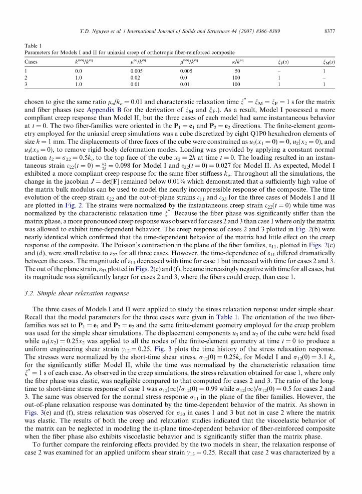
Table 1Parameters for Models I and II for uniaxial creep of orthotropic fiber-reinforced composite
Cases kneq/keq leq/keq lneq/keq j/keq nF(s) nM(s)
1 0.0 0.005 0.005 50 – 12 1.0 0.02 0.0 100 1 –3 1.0 0.01 0.01 100 1 1
T.D. Nguyen et al. / International Journal of Solids and Structures 44 (2007) 8366–8389 8377
chosen to give the same ratio lo/ko = 0.01 and characteristic relaxation time n* = nM = nF = 1 s for the matrixand fiber phases (see Appendix B for the derivation of nM and nF.). As a result, Model I possessed a morecompliant creep response than Model II, but the three cases of each model had same instantaneous behaviorat t = 0. The two fiber-families were oriented in the P1 = e1 and P2 = e2 directions. The finite-element geom-etry employed for the uniaxial creep simulations was a cube discretized by eight Q1P0 hexahedron elements ofsize h = 1 mm. The displacements of three faces of the cube were constrained as u1(x1 = 0) = 0, u2(x2 = 0), andu3(x3 = 0), to remove rigid body deformation modes. Loading was provided by applying a constant normaltraction t2 = r22 = 0.5ko to the top face of the cube x2 = 2h at time t = 0. The loading resulted in an instan-taneous strain e22ðt ¼ 0Þ ¼ u2
2h ¼ 0:098 for Model I and e22(t = 0) = 0.027 for Model II. As expected, Model Iexhibited a more compliant creep response for the same fiber stiffness ko. Throughout all the simulations, thechange in the jacobian J = det[F] remained below 0.01% which demonstrated that a sufficiently high value ofthe matrix bulk modulus can be used to model the nearly incompressible response of the composite. The timeevolution of the creep strain e22 and the out-of-plane strains e11 and e33 for the three cases of Models I and IIare plotted in Fig. 2. The strains were normalized by the instantaneous creep strain e22(t = 0) while time wasnormalized by the characteristic relaxation time n*. Because the fiber phase was significantly stiffer than thematrix phase, a more pronounced creep response was observed for cases 2 and 3 than case 1 where only the matrixwas allowed to exhibit time-dependent behavior. The creep response of cases 2 and 3 plotted in Fig. 2(b) werenearly identical which confirmed that the time-dependent behavior of the matrix had little effect on the creepresponse of the composite. The Poisson’s contraction in the plane of the fiber families, e11, plotted in Figs. 2(c)and (d), were small relative to e22 for all three cases. However, the time-dependence of e11 differed dramaticallybetween the cases. The magnitude of e11 decreased with time for case 1 but increased with time for cases 2 and 3.The out of the plane strain, e33 plotted in Figs. 2(e) and (f), became increasingly negative with time for all cases, butits magnitude was significantly larger for cases 2 and 3, where the fibers could creep, than case 1.
3.2. Simple shear relaxation response
The three cases of Models I and II were applied to study the stress relaxation response under simple shear.Recall that the model parameters for the three cases were given in Table 1. The orientation of the two fiber-families was set to P1 = e1 and P2 = e2 and the same finite-element geometry employed for the creep problemwas used for the simple shear simulations. The displacement components u3 and u2 of the cube were held fixedwhile u1(x2) = 0.25x2 was applied to all the nodes of the finite-element geometry at time t = 0 to produce auniform engineering shear strain c12 = 0.25. Fig. 3 plots the time history of the stress relaxation response.The stresses were normalized by the short-time shear stress, r12(0) = 0.25ko for Model I and r12(0) = 3.1 ko
for the significantly stiffer Model II, while the time was normalized by the characteristic relaxation timen* = 1 s of each case. As observed in the creep simulations, the stress relaxation obtained for case 1, where onlythe fiber phase was elastic, was negligible compared to that computed for cases 2 and 3. The ratio of the long-time to short-time stress response of case 1 was r12(1)/r12(0) = 0.99 while r12(1)/r12(0) = 0.5 for cases 2 and3. The same was observed for the normal stress response r11 in the plane of the fiber families. However, theout-of-plane relaxation response was dominated by the time-dependent behavior of the matrix. As shown inFigs. 3(e) and (f), stress relaxation was observed for r33 in cases 1 and 3 but not in case 2 where the matrixwas elastic. The results of both the creep and relaxation studies indicated that the viscoelastic behavior ofthe matrix can be neglected in modeling the in-plane time-dependent behavior of fiber-reinforced compositewhen the fiber phase also exhibits viscoelastic behavior and is significantly stiffer than the matrix phase.
To further compare the reinforcing effects provided by the two models in shear, the relaxation response ofcase 2 was examined for an applied uniform shear strain c13 = 0.25. Recall that case 2 was characterized by a

10—2 10—1 100 1011
1.0005
1.001
1.0015
1.002
1.0025
1.003
1.0035
Time (t/ξ*)
Cre
ep S
train
(ε22
/ε22
| t=0)
Model I, case 1Model II, case 1
a
10—2 10—1 100 1011
1.1
1.2
1.3
1.4
1.5
1.6
1.7
1.8
Time (t/ξ*)
Cre
ep S
train
(ε22
/ε22
| t=0)
Model I, case 2Model I, case 3Model II, case 2Model II, case 3
b
10—2 10—1 100 101—0.014
—0.012
—0.01
—0.008
—0.006
—0.004
—0.002
0
Time (t/ξ*)
ε 11/ε
22| t=
0
Model I, case 1Model I, case 2Model I, case 3
c
10—2 10—1 100 101—0.014
—0.012
—0.01
—0.008
—0.006
—0.004
—0.002
0
Time (t/ξ*)
ε 11/ε
22| t=
0
Model II, case 1Model II, case 2Model II, case 3
d
10—2 10—1 100 101—1.8
—1.6
—1.4
—1.2
—1
—0.8
Time (t/ξ*)
ε 33/ε
22| t=
0
Model I, case 1Model I, case 2Model I, case 3
e
10—2 10—1 100 101—1.8
—1.6
—1.4
—1.2
—1
—0.8
Time (t/ξ*)
ε 33/ε
22| t=
0
Model II, case 1Model II, case 2Model II, case 3
f
Fig. 2. Uniaxial tensile creep: (a) creep strain in the loading direction e22 for case 1 of both models, (b) e22 for cases 2 and 3 of both models,(c) e11 for all cases of Model I, (d) e11 for all cases of Model II, (e) e33 for all cases of Model I, and (f) e33 for all cases of Model II.
8378 T.D. Nguyen et al. / International Journal of Solids and Structures 44 (2007) 8366–8389
viscoelastic fiber phase and an elastic matrix phase. The shear strain was applied by specifying u2 = u3 = 0 andu1(x3) = 0.25x3 at all the nodes of the finite-element model. The stress response of Model I to c13 was com-pletely independent of time. The fiber families of Model I remained unstretched in this loading geometry,and the stress response of the composite was determined solely by the elastic matrix. In contrast, the fiber fam-ilies provided a reinforcing effect in Model II because the applied deformation induced a stretch in the higherorder invariant, I5 = 1 + c13. This enabled the relaxation of the stress response r13 and r11 shown in Fig. 4.
3.3. Inflation of composite tube
Model I was applied to simulate the inflation of a laminated thick-wall tube. A schematic of the compositetube is illustrated in Fig. 5. The thick-wall tube consisted of two laminates, each composed of two helically
10—2 10—1 100 1010.99
0.992
0.994
0.996
0.998
1
Time (t/ξ*)
Stre
ss R
elax
atio
n (σ
12/σ
12| t=
0)
Model I, case 1Model II, case 1
a
10—2 10—1 100 1010.5
0.6
0.7
0.8
0.9
1
Time (t/ξ*)
Stre
ss R
elax
atio
n (σ
12/σ
12| t=
0)
Model I, case 2Model I, case 3Model II, case 2Model II, case 3
b
10—2 10—1 100 1010
0.1
0.2
0.3
0.4
0.5
Time (t/ξ*)
σ 11/σ
12| t=
0
Model I, case 1Model I, case 2Model I, case 3
c
10—2 10—1 100 1010.5
0.6
0.7
0.8
0.9
1
Time (t/ξ*)
σ 11/σ
12| t=
0
Model II, case 1Model II, case 2Model II, case 3
d
10—2 10—1 100 101—3.5
—3
—2.5
—2
—1.5
—1 x 10—3
Time (t/ξ*)
σ 33/
33| t=
0)
Model I, case 1Model I, case 2Model I, case 3
e
10—2 10—1 100 101—3
—2.5
—2
—1.5
—1 x 10—4
Time (t/ξ*)
σ 33/σ
12| t=
0)
Model II, case 1Model II, case 2Model II, case 3
f
Fig. 3. Simple shear relaxation: (a) shear stress in the loading direction r12 for case 1 of both models, (b) r12 for cases 2 and 3 of bothmodels, (c) r11 for all cases of Model I, (d) r11 for all cases of Model II, (e) r33 for all cases of Model I, (f) r33 for all cases of Model II.
T.D. Nguyen et al. / International Journal of Solids and Structures 44 (2007) 8366–8389 8379
wound fiber families embedded in an isotropic matrix. The orientation of fiber families were symmetric withrespect to the tube axis. The geometry of the composite tube was chosen to represent the dimensions and fiberarrangement of the adventitia and media layers of a human elastic artery as provided by Holzapfel et al.(2002). However, the material parameters listed in Table 1 for case 3 were applied to model both laminates.A quarter model of the tube was constructed for the finite-element simulation and discretized using Q1P0mixed elements of length L/12 in the axial direction and p/52 rad in the circumferential direction. For eachlayer, the size of the elements in the radial direction was biased towards the center to capture the high stressgradients near the inner surface of each layers. In total, eight elements were used to discretize the radial thick-ness of the inner layer and four elements were used for the outer layer. The vertical displacement at the ends ofthe tube was constrained as u3(z = �L/2) = u3(z = L/2) = 0 to preclude axial stretching, and u3(x2 = 0) = 0and u1(x1 = 0) were set to preserve the radial symmetry of the quarter tube model. An internal pressure,

Fig. 5. Schematic of thick-wall cylinder composed of two laminates of different fiber windings. The tube is inflated by applying a cyclicinternal pressure while holding the ends fixed.
10—2 10—1 100 1010.5
0.6
0.7
0.8
0.9
1
Time (t/ξ*)
Shea
r Stre
ss R
elax
atio
n (σ
13/σ
13| t=
0)Model II, case 2
10—2 10—1 100 1012
2.5
3
3.5
4
4.5
5
Time (t/ξ*)
σ 11/σ
13
—
Model II, case 2a b
Fig. 4. Stress relaxation for Model II subject to simple shear out of the plane of the fiber families: (a) shear stress r13 along the loadingdirection, (b) normal stress r11 along the loading direction.
8380 T.D. Nguyen et al. / International Journal of Solids and Structures 44 (2007) 8366–8389
p(t), was applied to the inner surface of the tube, while the outer surface of the tube was left traction free. Theapplied internal pressure p was ramped quickly from zero at t = 0 to p = 0.1ko at t = 0.1n*, then cycled sinu-soidally at a frequency of x = 2p/n* = 1 Hz between 0 6 p 6 0.05ko. The applied internal pressure is plotted inFig. 6 as a function of the internal volume change calculated as r2
i =R2i , where ri and Ri were the deformed and
1 1.05 1.1 1.15—0.01
0
0.01
0.02
0.03
0.04
0.05
0.06
Internal Volume (ri2/Ri
2)
Inte
rnal
Pre
ssur
e (p
/ko)
a
1 1.1 1.2 1.3 1.4—1
0
1
2
3
4
Radial Distance (r/Ri)
Stre
ss
σrr/p
σθθ/p
b —
—
Fig. 6. Cyclic inflation of laminate cylinder: (a) internal pressure vs. volume change, (b) the radial and hoop stresses, rrr and rhh, as afunction of radial distance.
T.D. Nguyen et al. / International Journal of Solids and Structures 44 (2007) 8366–8389 8381
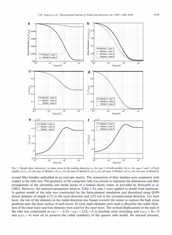
undeformed inner radius of the tube. For the applied frequency x = 1 Hz, steady-state was achieved in thepressure–volume response after one loading period. The steady-state pressure–volume curve formed an ellip-tical shape characteristic of the hysteresis curve of viscoelastic materials. The viscous dissipation can be com-puted by integrating the area underneath the steady-state pressure–volume curve for one cycle. The radial andhoop stress of the laminate cylinder are plotted in Fig. 6(b) as a function of the radial distance. The compres-sive radial stress decreased smoothly from the applied pressure �p at the internal surface R/Ri = 1 to zero atthe traction free external surface R/Ri = 1.43. Meanwhile, the tensile hoop stress decreased gradually from�3.8 6 rhh/p 6 �3.0 for 1.0 6 R/Ri 6 1.21, then more dramatically from �3.0 6 rhh/p 6 �0.93 for 1.0 6 R/Ri 6 1.32 before slowly decreasing to �rhh/p = �0.85 at the external surface of the cylinder, R/Ri = 1.43.The sharp decrease in the hoop stress occurred near the interface of the two laminates located at r/Ri = 1.29. The hoop stress was significantly higher in the inner laminate because the ±10� fiber winding anglesof the inner laminate provided a stiffer hoop reinforcement than the ±40� fiber winding of the outer layer.
4. Conclusion
A general constitutive framework has been presented for modeling the finite-deformation viscoelasticbehavior of soft fiber-reinforced composites. The essential and distinguishing features of the model includes:
• The parallel decomposition of the deformation gradient and additive split of the free energy density intomatrix and fiber components and then further into elastic/equilibrium and viscous/nonequilibrium compo-nents. This allows separate stress relations and viscous flow rules to be specified for the constituent phases.
• The mapping of the structure tensor to the intermediate configuration with the viscous deformation gradi-ent of the fiber phase which permits the fiber arrangement to be specified only in reference configuration.
• The definition of the viscous and elastic fiber stretch from the viscous and total deformation gradient of thefiber phase and the structure tensors.
• The formulation of one-dimensional viscous flow rules for the individual fiber families and the homogeni-zation of the individual flow rules for the three-dimensional.
The main result of this new approach is that it introduces a description of the fiber arrangement in the effec-tive viscous properties of the fiber phase in the same manner that the analogous homogenization scheme forthe free energy density incorporates a description of the fiber arrangement in the effective elastic properties. Anattractive feature of the approach to anisotropic viscoelasticity presented here is that key model parameterscan be related to the material properties (i.e., moduli and viscosities) of the constituent phases and to thearrangement of the fiber families. Consequently, the model parameters can be determined, when possible, fromindependent characterizations of the viscoelastic properties of the matrix and fiber materials and of the com-posite morphology. The formulation of the model also provides for a simple and efficient numerical implemen-tation in a finite-element framework. The constitutive relations depend only on the externally applied stretchand internal stretches, which are evaluated for the matrix and fiber phases in a finite-element framework at theintegration point level using a first-order accurate, stable Newton solution algorithm. Finally, the approachcan be extended to model anisotropic elasto-viscoplasticity for fiber-reinforced composites. An analogous elas-to-viscoplastic model would include the formulation for the individual fiber families of a yield condition usingthe fiber stress, a plastic flow rule for the plastic fiber stretch, and the Kuhn–Tucker conditions involving theplastic fiber stretch and the fiber yield condition. These features allow the constitutive models presented here toserve as an efficient and predictive simulation tool for the design and analysis of a class of materials that isimportant in both engineering applications and in biomechanics. In the area of biomechanics, the model isapplied currently to study the viscoelastic behavior of the cornea (Nguyen et al., submitted for publication).In addition, its application to modeling the viscoelastic behavior of blood vessels is being explored.
Acknowledgements
We thank Dr. D. Bammann and Prof. R. Ogden for insightful discussions on continuum theories of mod-eling material anisotropy and inelasticity under finite-deformations. This work was funded by the Laboratory
8382 T.D. Nguyen et al. / International Journal of Solids and Structures 44 (2007) 8366–8389
Directed Research and Development program at Sandia National Laboratories. Sandia is a multiprogram lab-oratory operated by Sandia Corporation, a Lockheed Martin Company, for the United States Department ofEnergy under contract DE-ACO4-94AL85000.
Appendix A. Numerical implementation
The constitutive relations for the two models presented in Sections 2.3 and 2.4 require the integrationof the isotropic evolution equation for Cv
M of the matrix and the anisotropic evolution equation for CvF
of the fiber phase. An efficient numerical integration algorithm has been developed by Reese and Gov-indjee (1998) for the spatial representation of the isotropic evolution Eq. (24). Their work also providesa method for calculating the consistent tangent for the isotropic component of the stress response.Therefore, this section will focus only on developing integration algorithms for the anisotropic evolutionequations for Cv
F and the material tangent for the anisotropic nonequilibrium component of the stressresponse.
A.1. Numerical integration of the evolution equations
In a finite-element framework, the time integration of the evolution equations for the internal vari-ables are performed at the integration point level. At time tn+1 = tn + Dt, the updated internal variablesare evaluated assuming that the updated values of the deformation gradient Fn+1 are given and that theprevious values of the deformation gradient Fn, previous values of the internal variables Cv
Mnand Cv
Fn,
and the structure tensors Ma are known. For the constitutive model presented in Section 2.3 for N fiber-families, the flow rule in Eq. (29) for kv
a can be integrated numerically using a backward Euler integra-tion scheme. Applying the time discretization of the viscous stretch rate _kv
a ¼ ðkvanþ1� kv
anÞ=Dt to Eq. (29)
gives
kvanþ1� Dt
gFaðka; k
vaÞ
sneqFaðke
a�
nþ1
kvanþ1� kv
an¼ 0; ðA:1Þ
where it has been assumed that the fiber viscosity, gFa, can depend generally on the total and viscous stretch, ka
and kva. The N nonlinear equations are solved at each integration point for the updated values kv
anþ1using the
Newton solution algorithm presented in Table A.1.For the case where there are more than three fiber families arranged in a plane, and more than six fiber
families in a fully three-dimensional arrangement, it is more efficient to solve for CvF rather than for the viscous
fiber stretches. The rate Eq. (30) is inverted to give an evolution equation for CvF,
_CvF ¼ 2V�1
F : TF; ðA:2Þ
where the fourth-order viscosity tensor VF given in Eq. (30) is required to be invertible. A backward Eulerdiscretization scheme is applied to Eq. (A.2) to give
CvFnþ1� 2DtV�1
Fnþ1TFnþ1
� CvFn¼ 0: ðA:3Þ
Eq. (A.3) is a nonlinear equation for the updated values of CvF that is solved at the integration point using the
Newton scheme presented in Table A.2.Similarly, for the generalized two fiber-families model presented in Section 2.4, a backward Euler integra-
tion scheme is applied to discretize the evolution Eq. (39) for the fiber viscous deformation. This results in thefollowing nonlinear system of equations for Cv
Fnþ1,
CvFnþ1�X2
a¼1
2DtgFaðkanþ1
; kvanþ1Þ TFnþ1
: sym MaCvFnþ1
h i� �sym MaCv
Fnþ1
h i� Cv
Fn¼ 0: ðA:4Þ
This is solved at each integration point using the Newton solution algorithm described in Table A.3.

Table A.2Integration algorithm for Cv
Fnþ1for N fiber-families model
Residual k + 1 iteration: Rkþ1 ¼ Cvkþ1
F � 2DtðVkþ1F Þ
�1 : Tkþ1F � Cv
Fn¼ 0
TF ¼PN
a¼1sneqFa
MaCv
F :Ma
VF ¼P2
a¼1gFa
kv4
Fa
Ma �Ma
Linearize about Cvk
Fnþ1: Rkþ1 � Rk þ oR
oCvF
����|ffl{zffl}K
CvkF
DCvF ¼ 0
Consistent tangent: K ¼ I� DtV�1F : 2 oTF
oCvF�PN
a1kv
a
ogFaokv
aMi : V�1
F : TF
� �Ma �Ma
� �2 oTF
oCvF¼PN
a¼1 � 2osneq
FaoIe
F2aþ2
IeFa
MaCv
F :Ma� Ma
CvF :Ma
Solve for the increment: DCvF ¼ �K�1 : Rk
CvkF
���Update solution: Cvkþ1
F ¼ Cvk
F þ DCvF
Repeat until: kRk+1k < ctol
Increment of CvF: DCv
F ¼ K�1 : G : DC
G ¼ DtV�1F : 2 oTF
oC�PN
i1ka
ogFaoka
Ma : V�1F : TF
� �Ma �Ma
� �\
2 oTF
oC¼PN
a¼12osneq
FaoIe
F2aþ2
MaCv
F :Ma� Ma
CvF :Ma
Algorithmic moduli: CneqF ¼ 2
oSneqF
oCþ 2
oSneqF
oCvF
: K�1 : G
2oS
neqF
oC¼PN
a¼14oWneq
FaoIe
F2aþ2
MaCv
F :Ma� Ma
CvF :Ma
2oS
neqF
oCvF¼PN
a¼1 � 2osneq
FaoIe
F2aþ2
MaCv
F :Ma� Ma
CvF :Ma
Table A.1Integration algorithm for kv
anþ1for N fiber-families model
Residual for k + 1 iteration: rkþ1a ¼ kvkþ1
a � Dtgkþ1
Fa
sneqk
Fakvkþ1
a � kvan¼ 0
sneqFa¼ 2
oWneqF
oIeFaþ3
IeFaþ3
Linearize about kvk
Fanþ1: rkþ1
a � rka kv
Fa
� �þ ora
okva
����|{z}ka
kvka
Dkvi ¼ 0
Consistent tangent: ka ¼ 1� DtgFa
1� 1gFa
ogFaokv
akv
a
� �sneq
Fa� 2
osneqFa
oIeFaþ3
IeFaþ3
� �Solve for the increment: Dkv
a ¼ � raka kvk
a
���Update solution: kvkþ1
a ¼ kvk
a þ Dkva
Repeat until: rkþ1a < ctol
Increment of CvF: DCv
F : Ma ¼ gakak
eaDC : Ma
ga ¼ � DtgFa
1gFa
ogFaoka
kasneqFa� 2
osneqFa
oIeFaþ3
IeFaþ3
� �kv
aka
Algorithmic moduli: CneqF ¼
PNa¼1 4
o2WneqFa
oIe2
Faþ3
� 4o2W
neqFa
oIe2
Faþ3
IeFaþ3þ oW
neqFa
oIeFaþ3
� �ga
ka
ffiffiffiffiffiffiffiffiIe
Faþ3
p !Ma
CvF :Ma� Ma
CvF :Ma
T.D. Nguyen et al. / International Journal of Solids and Structures 44 (2007) 8366–8389 8383
A.2. Consistent tangent moduli
The implicit solution of an initial boundary value problem requires the time discretization of the deforma-tion history and linearization of the constitutive relations about the deformation state at time tn to solve forthe updated deformation state at time tn+1 = tn + D t. The consistent material tangent moduli is defined by thelinearization of the second Piola–Kirchhoff stress response for a time increment Dt as
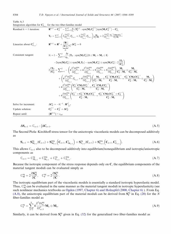
Table A.3Integration algorithm for Cv
Fnþ1for the two fiber-families model
Residual k + 1 iteration: Rkþ1 ¼ Cvkþ1
F �P2
a¼1DtgFaðTkþ1
F : sym½MaCvkþ1
F �Þsym½MaCvkþ1
F � � CvFn
TF ¼P2
a¼1 2oWneq
FaoIe
F2aþ2
IeF2aþ2þ 2
oWneqFa
oIeF2aþ3
IeF2aþ3
� �Ma
CvF :Maþ 2
oWneqFa
oIeF2aþ3
Cv�1
F CMaCCv�1
F
CvF :Ma
Linearize about Cvk
Fnþ1: Rkþ1 � Rk þ oR
oCvF
����|ffl{zffl}K
CvkF
DCvF ¼ 0
Consistent tangent: K ¼ I�X2
a¼1
DtgFa
TF : sym½MaCvF�ð1�Ma þMa � 1Þ
��2sym½MaCv
F� � sym½MaTF� � sym½MaCvF� � sym½MaCv
F� : 2oTF
oCvF
�2
oTF
oCvF
¼X2
a¼1� 4
o2WneqF
oIe2
F2aþ2
þ 4o2W
neqF
oIe2
F2aþ3
þ 8oW
neqF
oIeF2aþ2
þ 8oW
neqF
oIeF2aþ3
!Ma
CvF : Ma
� Ma
CvF : Ma
þ 4o2W
neqF
oIe2
F2aþ2
IeF2aþ3þ 4
oWneqF
oIeF2aþ3
!Ma
CvF : Ma
� Cv�1
F CMaCCv�1
F
CvF : Ma
þ Cv�1
F CMaCCv�1
F
CvF : Ma
� Ma
CvF : Ma
!
þ 4o2W
neqF
oIe2
F2aþ3
Cv�1
F CMaCCv�1
F
CvF : Ma
� Cv�1
F CMaCCv�1
F
CvF : Ma
!
þ 4oW
neqF
oIeF2aþ3
Cv�1
F � Cv�1
F CMaCCv�1
F
CvF : Ma
þ Cv�1
F CMaCCv�1
F � Cv�1
F
CvF : Ma
!
Solve for increment: DCvF ¼ �K�1 : Rk
kvki
���Update solution: Cvkþ1
F ¼ Cvk
F þ DCvF
Repeat until: kRk+1k < ctol
8384 T.D. Nguyen et al. / International Journal of Solids and Structures 44 (2007) 8366–8389
DSnþ1 ¼ Cnþ1 : 12DCnþ1: ðA:5Þ
The Second Piola–Kirchhoff stress tensor for the anisotropic viscoelastic models can be decomposed additivelyas
Snþ1 ¼ SeqMnþ1ðCnþ1Þ þ Sneq
Mnþ1Cnþ1;C
vMnþ1
� �þ Seq
Fnþ1ðCnþ1Þ þ Sneq
Fnþ1Cnþ1;C
vFnþ1
� �: ðA:6Þ
This allows Cnþ1 also to be decomposed additively into equilibrium/nonequilibrium and isotropic/anisotropiccomponents as
Cnþ1 ¼ CeqMnþ1þ C
neqMnþ1þ C
eqFnþ1þ C
neqFnþ1
: ðA:7Þ
Because the isotropic component of the stress response depends only on C, the equilibrium components of thematerial tangent moduli can be evaluated simply as
CeqM ¼ 2
oSeqM
oC; C
eqF ¼ 2
oSeqF
oC: ðA:8Þ
The isotropic equilibrium part of the viscoelastic models is essentially a standard isotropic hyperelastic model.Thus, C
eqM can be evaluated in the same manner as the material tangent moduli in isotropic hyperelasticity (see
such nonlinear mechanics textbooks as Ogden (1997, Chapter 6) and Holzapfel (2000, Chapter 6) ). From Eq.(A.8), the anisotropic equilibrium part of the material moduli can be derived from S
eqF in Eq. (20) for the N
fiber-families model as
CeqF ¼
XN
a¼1
4o2Weq
Fa
oI2aþ3
Ma �Ma: ðA:9Þ
Similarly, it can be derived from SeqF given in Eq. (32) for the generalized two fiber-families model as
T.D. Nguyen et al. / International Journal of Solids and Structures 44 (2007) 8366–8389 8385
CeqF ¼
X2
a¼1
4o2Weq
Fa
oI22aþ2
Ma�MaþX2
a¼1
4o2Weq
Fa
oI22aþ3
ðCMaþMaCÞ�ðCMaþMaCÞþ4oWeq
Fa
oI2aþ3
ð1�MaþMa�1Þ !
;
ðA:10Þ
where the tensor in the final expression is defined as ð1�MÞIJKL ¼ 12ðdIKMJL þ dILMJKÞ.
The isotropic nonequilibrium part of the model is identical to the isotropic viscoelastic model developed byReese and Govindjee (1998) and it is recommended that their numerical method be applied to solve for theinternal stretches of the spatial form of the evolution Eq. (24) and to derive the material tangent moduliC
neqM . The anisotropic nonequilibrium part of the material moduli is evaluated by first linearizing the aniso-
tropic nonequilibrium component of the stress response SneqF as
DSneqF ¼ 2
oSneqF
oC:
1
2DCþ 2
oSneqF
oCvF
:1
2DCv
F: ðA:11Þ
Determining CneqF in Eq. (A.11) requires developing a relationship between the increment DCv
F of the fiberphase, which is solved locally at the integration point, and the increment DC of the global solution algorithm.For the N fiber-families model, this relationship can be determined for the integration algorithm described inTable A.1 by linearizing the residual equation raðkanþ1
; kvanþ1Þ ¼ 0. Considering that kanþ1
is not a constant in theglobal solution algorithm, this yields
ora
okva|{z}
ka
Dkva þ
ora
oka|{z}�ga
Dka ¼ 0;
DCvF : Ma ¼
ga
kakea
DC : Ma; ðA:12Þ
where the expressions for ka and ga are given in Table A.1. Substituting the final relation into Eq. (A.11) andfactoring out DC gives
CneqF ¼
XN
a¼1
4o
2WneqFa
oIe2
Faþ3
� 4o
2WneqFa
oIe2
Faþ3
IeFaþ3þ
oWneqFa
oIeFaþ3
!ga
ka
ffiffiffiffiffiffiffiffiffiIe
Faþ3
q0B@
1CA Ma
CvF : Ma
� Ma
CvF : Ma
: ðA:13Þ
Similarly, for the integration algorithms presented in Tables A.2 and A.3, a relationship for the the incrementDCv
Fnþ1is obtained by linearizing the residual equation RðCv
Fnþ1;Cnþ1Þ ¼ 0 for a non-constant Cn+1. The result,
DCvF ¼ K�1 : G : DC; ðA:14Þ
is substituted into Eq. (A.12) to give the following general expression for the anisotropic nonequilibrium com-ponent of the material tangent moduli,
CneqF ¼ 2
oSneqF
oCþ 2
oSneqF
oCvF
: K�1 : G: ðA:15Þ
The tensors K and G are specific to the solution algorithm of CvFnþ1
and are given in Table A.2 for the N fiber-families model and in Table A.4 for the generalized two fiber-families model.
Appendix B. Linearization for the small-strain limit
This section presents the linearization of the examples Model I and II presented in Section 3 to obtainexpressions for the long- and short-time moduli and characteristic relaxation times in the small-strain limit.For both models, the isotropic stress response of the matrix, rM, is obtained by substituting Eq. (41) intoEq. (21) to give
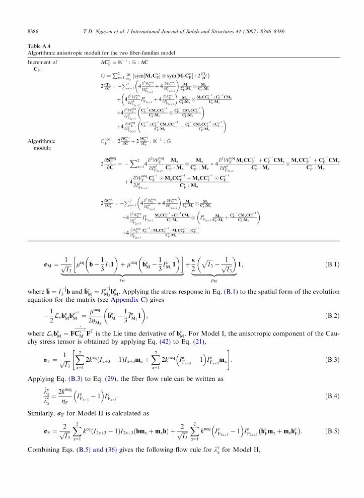
Table A.4Algorithmic anisotropic moduli for the two fiber-families model
Increment ofCv
F:DCv
F ¼ K�1 : G : DC
G ¼P2
a¼1DtgFa
sym½MaCvF� � sym½MaCv
F� : 2 oTF
oC
� �2 oTF
oC ¼ �P2
a¼1 4o2Wneq
F
oIe2
F2aþ2
þ 4oWneq
F
oIeF2aþ2
� �Ma
CvF :Ma� Ma
CvF :Ma
þ 4o2W
neqF
oIe2
F2aþ2
IeF2aþ3þ 4
oWneqF
oIeF2aþ3
� �Ma
CvF :Ma� MaCCv�1
F þCv�1
F CMa
CvF :Ma
þ4o2W
neqF
oIe2
F2aþ3
Cv�1
F CMaCCv�1
F
CvF :Ma
� Cv�1
F CMaCCv�1
F
CvF :Ma
� �þ4
oWneqF
oIeF2aþ3
Cv�1
F �Cv�1
F CMaCCv�1
F
CvF :Ma
þ Cv�1
F CMaCCv�1
F �Cv�1
F
CvF :Ma
� �Algorithmic
moduli:C
neqF ¼ 2
oSneqF
oCþ 2
oSneqF
oCvF
: K�1 : G
2oS
neqF
oC¼ �
X2
a¼14o2Wneq
F
oIe2
F2aþ2
Ma
CvF : Ma
� Ma
CvF : Ma
� 4o2Wneq
F
oIe2
F2aþ3
MaCCv�1
F þ Cv�1
F CMa
CvF : Ma
�MaCCv�1
F þ Cv�1
F CMa
CvF : Ma
þ 4oW
neqF
oIeF2aþ3
Cv�1
F �MaCCv�1
F þMaCCv�1
F � Cv�1
F
CvF : Ma
2oS
neqF
oCvF¼ �
P2a¼1 4
o2WneqF
oIe2
F2aþ2
þ 4oWneq
F
oIeF2aþ2
� �Ma
CvF :Ma� Ma
CvF :Ma
þ4o2W
neqF
oIe2
F2aþ3
IeF2aþ3
MaCCv�1
F þCv�1
F CMa
CvF :Ma
� IeF2aþ3
MaCv
F :Maþ Cv�1
F CMaCCv�1
F
CvF :Ma
� �þ4
oWneqF
oIeF2aþ3
Cv�1
F �MaCCv�1
F þMaCCv�1
F �Cv�1
F
CvF :Ma
8386 T.D. Nguyen et al. / International Journal of Solids and Structures 44 (2007) 8366–8389
rM ¼1ffiffiffiffiI3
p leq �b� 1
3�I11
� �þ lneq �be
M �1
3�Ie
M11
� �� |fflfflfflfflfflfflfflfflfflfflfflfflfflfflfflfflfflfflfflfflfflfflfflfflfflfflfflfflfflfflfflfflfflfflfflfflfflfflfflffl{zfflfflfflfflfflfflfflfflfflfflfflfflfflfflfflfflfflfflfflfflfflfflfflfflfflfflfflfflfflfflfflfflfflfflfflfflfflfflfflffl}
sM
þ j2
ffiffiffiffiI3
p� 1ffiffiffiffi
I3
p� �|fflfflfflfflfflfflfflfflfflfflfflfflffl{zfflfflfflfflfflfflfflfflfflfflfflfflffl}
pM
1; ðB:1Þ
where �b ¼ I�1
33 b and �be
M ¼ I e�1
3
M3be
M. Applying the stress response in Eq. (B.1) to the spatial form of the evolutionequation for the matrix (see Appendix C) gives
� 1
2Lvbe
Mbe�1
M ¼ lneq
2gMS
�beM �
1
3�Ie
M11
� �; ðB:2Þ
where LvbeM ¼ F
_Cv�1
M FT is the Lie time derivative of beM. For Model I, the anisotropic component of the Cau-
chy stress tensor is obtained by applying Eq. (42) to Eq. (21),
rF ¼1ffiffiffiffiI3
pX2
a¼1
2keqðIaþ3 � 1ÞIaþ3ma þX2
a¼1
2kneq IeFaþ3� 1
� �I e
Faþ3ma
" #: ðB:3Þ
Applying Eq. (B.3) to Eq. (29), the fiber flow rule can be written as
_kva
kva
¼ 2kneq
gF
IeFaþ3� 1
� �Ie
Faþ3: ðB:4Þ
Similarly, rF for Model II is calculated as
rF ¼2ffiffiffiffiI3
pX2
a¼1
keqðI2aþ3 � 1ÞI2aþ3ðbma þmabÞ þ 2ffiffiffiffiI3
pX2
a¼1
kneq IeF2aþ3� 1
� �Ie
F2aþ3be
Fma þmabeF
� �: ðB:5Þ
Combining Eqs. (B.5) and (36) gives the following flow rule for kva for Model II,

T.D. Nguyen et al. / International Journal of Solids and Structures 44 (2007) 8366–8389 8387
_kva
kva
¼ 2
gF
kneq IeF2aþ3� 1
� �Ie
F2aþ3þX2
b
Cv�1
F CMb : MaC
CvF : Mb
þMbCCv�1
F : CMa
CvF : Mb
! !: ðB:6Þ
To examine the small strain behavior of the two models, the linearized Green–Lagrange strain is defined ase ¼ 1
2ðC� 1Þ and the associated linearized elastic and viscous strain tensors are defined as ev ¼ 1
2ðCv � 1Þ
and ee = e � ev for both the matrix and fiber phases. Moreover, the structure tensor in the various configura-tion reduces in the small-strain limit to ma ! fMa !Ma. In the limit of small strains, the models reduces to athree-dimensional generalization of the rheological model shown in Fig. 1 of two standard three parametermodels arranged in parallel. Separately, the two standard models describe the viscoelastic behavior of the ma-trix and fiber phases and their parallel combination describes the viscoelastic behavior of the composite. Thestrain e is the total strain of the rheological model, while ee
M and eeF are the strains of the springs in the Maxwell
elements. The linearized evolution equations developed below for the viscous strains evM and ev
F govern the flowof the dashpots in the two Maxwell elements representing the relaxation of the matrix and fiber phases.
The small-strain short-time stress response (t! 0) of Model I is computed by linearizing Eqs. (B.1) and(B.3) in the limit ee
M ! eeF ! e to give
ro ¼ ð2ðleq þ lneqÞ I� 1
31� 1
� �þ j1� 1þ
X2
a¼14ðkeq þ kneqÞMa �MaÞ|fflfflfflfflfflfflfflfflfflfflfflfflfflfflfflfflfflfflfflfflfflfflfflfflfflfflfflfflfflfflfflfflfflfflfflfflfflfflfflfflfflfflfflfflfflfflfflfflfflfflfflfflfflfflfflfflfflfflfflfflfflfflfflfflfflffl{zfflfflfflfflfflfflfflfflfflfflfflfflfflfflfflfflfflfflfflfflfflfflfflfflfflfflfflfflfflfflfflfflfflfflfflfflfflfflfflfflfflfflfflfflfflfflfflfflfflfflfflfflfflfflfflfflfflfflfflfflfflfflfflfflfflffl}
co
: e: ðB:7Þ
The tensor co is defined as the small-strain short-time moduli. Similarly, the small-strain long-time (t!1)stress response of Model I is computed by linearizing Eqs. (B.1) and (B.3) in the limit ev
M ! evF ! e to yield
r1 ¼ 2leq I� 1
31� 1
� �þ j1� 1þ
X2
a¼14keqMa �Ma
� �|fflfflfflfflfflfflfflfflfflfflfflfflfflfflfflfflfflfflfflfflfflfflfflfflfflfflfflfflfflfflfflfflfflfflfflfflfflfflfflfflfflfflfflfflfflfflfflfflfflffl{zfflfflfflfflfflfflfflfflfflfflfflfflfflfflfflfflfflfflfflfflfflfflfflfflfflfflfflfflfflfflfflfflfflfflfflfflfflfflfflfflfflfflfflfflfflfflfflfflfflffl}
c1
: e: ðB:8Þ
The short- and long-time small-strain moduli can be computed for Model II in the same manner to give
co ¼ 2ðleq þ lneqÞ I� 1
31� 1
� �þ j1� 1þ
X2
a¼1
16 keq þ kneqð ÞMa �Ma;
c1 ¼ 2leq I� 1
31� 1
� �þ j1� 1þ
X2
a¼1
16kneqMa �Ma: ðB:9Þ
To obtain the characteristic relaxation time of the matrix, Eq. (B.2) is linearized as
_evM ¼
1
nM
I� 1
31� 1
� �: ee
M; ðB:10Þ
where evM ¼ ev
M � trðevMÞ1, and e e
M ¼ eeM � trðee
MÞ1 are the deviatoric strain components. The parameternM ¼ gMS
=lneq is the characteristic relaxation time of the matrix. The characteristic relaxation time of the fiberphase is obtained for Models I and II by linearizing Eqs. (B.4) and (B.6). The result can be expressed as
_evF : Ma ¼
1
nF
eeF : Ma; ðB:11Þ
where nF = gF/(4kneq) is the characteristic relaxation time of the fiber phase for Model I and nF = gF/(16kneq)is for Model II.
Appendix C. Viscoelastic evolution of the matrix phase
The following demonstrates that the spatial representation of Eq. (24) is identical to the evolution equationdeveloped for the isotropic viscoelasticity theory of Reese and Govindjee (1998). First the evolution Eq. (24) isrewritten as follows,
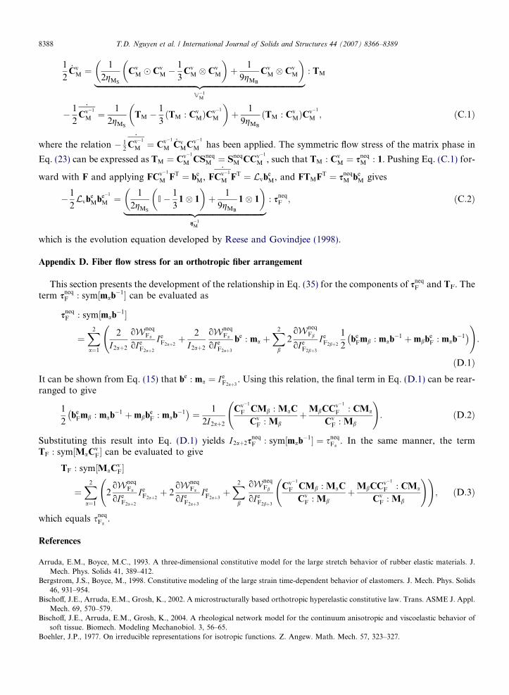
8388 T.D. Nguyen et al. / International Journal of Solids and Structures 44 (2007) 8366–8389
1
2_Cv
M ¼1
2gMS
CvM � Cv
M �1
3Cv
M � CvM
� �þ 1
9gMB
CvM � Cv
M
� �|fflfflfflfflfflfflfflfflfflfflfflfflfflfflfflfflfflfflfflfflfflfflfflfflfflfflfflfflfflfflfflfflfflfflfflfflfflfflfflfflfflfflfflfflfflfflfflfflfflffl{zfflfflfflfflfflfflfflfflfflfflfflfflfflfflfflfflfflfflfflfflfflfflfflfflfflfflfflfflfflfflfflfflfflfflfflfflfflfflfflfflfflfflfflfflfflfflfflfflfflffl}
V�1M
: TM
� 1
2
_Cv�1
M ¼ 1
2gMS
TM �1
3ðTM : Cv
MÞCv�1
M
� �þ 1
9gMB
ðTM : CvMÞC
v�1
M ; ðC:1Þ
where the relation � 12
_Cv�1
M ¼ Cv�1
M_Cv
MCv�1
M has been applied. The symmetric flow stress of the matrix phase in
Eq. (23) can be expressed as TM ¼ Cv�1
M CSneqM ¼ Sneq
M CCv�1
M , such that TM : CvM ¼ s
neqM : 1. Pushing Eq. (C.1) for-
ward with F and applying FCv�1
M FT ¼ beM, F
_Cv�1
M FT ¼ LvbeM, and FTMFT ¼ s
neqM be
M gives
� 1
2Lvbe
Mbe�1
M ¼ 1
2gMS
I� 1
31� 1
� �þ 1
9gMB
1� 1
� �|fflfflfflfflfflfflfflfflfflfflfflfflfflfflfflfflfflfflfflfflfflfflfflfflfflfflfflfflfflfflfflfflffl{zfflfflfflfflfflfflfflfflfflfflfflfflfflfflfflfflfflfflfflfflfflfflfflfflfflfflfflfflfflfflfflfflffl}
g�1M
: sneqF ; ðC:2Þ
which is the evolution equation developed by Reese and Govindjee (1998).
Appendix D. Fiber flow stress for an orthotropic fiber arrangement
This section presents the development of the relationship in Eq. (35) for the components of sneqF and TF. The
term sneqF : sym½mab�1� can be evaluated as
sneqF : sym½mab�1�
¼X2
a¼1
2
I2aþ2
oWneqFa
oIeF2aþ2
IeF2aþ2þ 2
I2aþ2
oWneqFa
oIeF2aþ3
be : ma þX2
b
2oWneq
Fb
oI eF2bþ3
I eF2bþ2
1
2be
Fmb : mab�1 þmbbeF : mab�1
� � !:
ðD:1Þ
It can be shown from Eq. (15) that be : ma ¼ IeF2aþ3. Using this relation, the final term in Eq. (D.1) can be rear-
ranged to give
1
2be
Fmb : mab�1 þmbbeF : mab�1
� �¼ 1
2I2aþ2
Cv�1
F CMb : MaC
CvF : Mb
þMbCCv�1
F : CMa
CvF : Mb
!: ðD:2Þ
Substituting this result into Eq. (D.1) yields I2aþ2sneqF : sym½mab�1� ¼ sneq
Fa. In the same manner, the term
TF : sym½MaCvF� can be evaluated to give
TF : sym½MaCvF�
¼X2
a¼1
2oWneq
Fa
oI eF2aþ2
IeF2aþ2þ 2
oWneqFa
oIeF2aþ3
IeF2aþ3þX2
b
oWneqFb
oIeF2bþ3
Cv�1
F CMb : MaC
CvF : Mb
þMbCCv�1
F : CMa
CvF : Mb
! !; ðD:3Þ
which equals sneqFa
.
References
Arruda, E.M., Boyce, M.C., 1993. A three-dimensional constitutive model for the large stretch behavior of rubber elastic materials. J.Mech. Phys. Solids 41, 389–412.
Bergstrom, J.S., Boyce, M., 1998. Constitutive modeling of the large strain time-dependent behavior of elastomers. J. Mech. Phys. Solids46, 931–954.
Bischoff, J.E., Arruda, E.M., Grosh, K., 2002. A microstructurally based orthotropic hyperelastic constitutive law. Trans. ASME J. Appl.Mech. 69, 570–579.
Bischoff, J.E., Arruda, E.M., Grosh, K., 2004. A rheological network model for the continuum anisotropic and viscoelastic behavior ofsoft tissue. Biomech. Modeling Mechanobiol. 3, 56–65.
Boehler, J.P., 1977. On irreducible representations for isotropic functions. Z. Angew. Math. Mech. 57, 323–327.

T.D. Nguyen et al. / International Journal of Solids and Structures 44 (2007) 8366–8389 8389
Boehler, J.P., 1979. A simple derivation of representation for non-polynomial constitutive equations in some cases of anisotropy. Z.Angew. Math. Mech. 59, 157–167.
Coleman, B.D., Gurtin, M.E., 1967. Thermodynamics with internal state variables. J. Chem. Phys. 47, 597–613.Ericksen, J.L., Rivlin, R.S., 1954. Large elastic deformations of homogeneous anisotropic materials. Arch. Ration. Mech. Anal. 3, 281–
301.Flory, P.J., 1961. Thermodynamic relations for highly elastic materials. Trans. Faraday Soc. 57, 829–838.Fung, Y.C., 1993. Biomechanics: Mechanical Properties of Living Tissues. Springer-Verlag, New York, NY.Govindjee, S., Reese, S., 1997. A presentation and comparison of two large deformation viscoelasticity models. Trans. ASME J. Eng.
Mater. Technol. 119, 251–255.Green, M.S., Tolbosky, A.V., 1946. A new approach to the theory of relaxing polymeric media. J. Comp. Phys. 14, 80–92.Holzapfel, G.A., 1996. On large strain viscoelasticity: continuum formulation and finite element applications to elastomeric structures. Int.
J. Numer. Methods Eng. 39, 3903–3926.Holzapfel, G.A., 2000. Nonlinear Solid Mechanics: A Continuum Approach for Engineers. John Wiley and Sons LTD, Chichester.Holzapfel, G.A., Gasser, T.C., 2000. A new constitutive framework for arterial wall mechanics and a comparative study of material
models. J. Elasticity 61, 1–48.Holzapfel, G.A., Gasser, T.C., Stadler, M., 2002. A structural model for the viscoelastic behavior of arterial walls: continuum formulation
and finite element analysis. Eur. J. Mech. A Solids 21, 441–463.Huang, K., 1950. On the atomistic theory of elasticity. Proc. R. Soc. Lond. A Math. Phys. Eng. Sci. 203, 178–194.Klinkel, S., Sansour, C., Wagner, W., 2005. An anisotropic fiber-matrix material model at finite elastic–plastic strains. Comput. Mech. 35,
409–417.Lanir, Y., 1983. Constitutive equations for fibrous connective tissues. J. Biomech. 16, 1–12.Limbert, G., Middleton, J., 2004. A transversely isotropic viscohyperelastic material: application to the modeling of biological soft
connective tissues. Int. J. Solids Struct. 2004, 4237–4260.Lion, A., 1996. A constitutive model for carbon black filled rubber. Experimental investigations and mathematical representations.
Continuum Mech. Thermodyn. 8, 153–169.Liu, S., 1982. On representations of anisotropic invariants. Int. J. Eng. Sci. 20, 1099–1109.Lubliner, J., 1985. A model of rubber viscoelasticity. Mech. Res. Commun. 12, 93–99.Merodio, J., Ogden, R.W., 2005. Mechanical response of fiber-reinforced incompressible non-linearly elastic solids. Int. J. Non-Linear
Mech. 40, 213–227.Nguyen, T.D., Govindjee, S.A., Klein, P., Gao, H., 2004. A rate-dependent cohesive continuum model for crack dynamics. Comput.
Methods Appl. Mech. Eng. 193, 3239–3265.Nguyen, T.D., Boyce, B.L., Jones, R.E. An anisotropic nonlinear viscoelastic model for the tensile behavior of the cornea. J. Biomech.
Eng., submitted for publication.Ogden, R.W., 1978. Nearly isochoric elastic deformations: application to rubber-like solids. J. Mech. Phys. Solids 26, 37–57.Ogden, R.W., 1997. Non-linear Elastic Deformations. Dover Publications, Inc, Mineola, NY.Pioletti, D.P., Rakotomanana, L.R., Benvnuti, J.F., Leyvraz, P.F., 1998. Viscoelastic constitutive law in large deformations: application to
human knee ligaments and tendons. J. Biomech. 31, 753–757.Reese, S., 2003. Meso-macro modelling of fibre-reinforced rubber-like composites exhibiting large elastoplastic deformation. Int. J. Solids
Struct. 40, 951–980.Reese, S., Govindjee, S., 1998. A theory of finite viscoelasticity and numerical aspects. Int. J. Solids Struct. 35, 3455–3482.Sansour, C., Bocko, J., 2003. On the numerical implications of multiplicative inelasticity with an anisotropic elastic constitutive law. Int. J.
Numer. Methods Eng. 58, 2131–2160.Simo, J.C., Taylor, R.L., Pister, K.S., 1985. Variational and projection methods for the volume constraint in finite deformation elasto-
plasticity. Comput. Methods Appl. Mech. Eng. 51, 177–208.Spencer, A.J.M., 1971. Theory of invariants. In: Eringen, A. (Ed.), . In: Continuum Physics, vol. I. Academic Press, New York, pp. 239–
353.Wang, C.C., 1969. On a general representation theorem for constitutive relations. Arch. Ration. Mech. Anal. 33, 1–25.