Swansea University E-Theses _________________________________________________________________________

Analysis of adaptive finite element solutions in elastoplasticity with

reference to transfer operation techniques.

Orlando, Antonio

How to cite: _________________________________________________________________________ Orlando, Antonio (2002) Analysis of adaptive finite element solutions in elastoplasticity with reference to transfer

operation techniques.. thesis, Swansea University.

http://cronfa.swan.ac.uk/Record/cronfa42476

Use policy: _________________________________________________________________________ This item is brought to you by Swansea University. Any person downloading material is agreeing to abide by the terms

of the repository licence: copies of full text items may be used or reproduced in any format or medium, without prior

permission for personal research or study, educational or non-commercial purposes only. The copyright for any work

remains with the original author unless otherwise specified. The full-text must not be sold in any format or medium

without the formal permission of the copyright holder. Permission for multiple reproductions should be obtained from

the original author.

Authors are personally responsible for adhering to copyright and publisher restrictions when uploading content to the

repository.

Please link to the metadata record in the Swansea University repository, Cronfa (link given in the citation reference

above.)

http://www.swansea.ac.uk/library/researchsupport/ris-support/

U n i v e r s i t y o f W a l e s S w a n s e a

S c h o o l o f E n g i n e e r i n g

a n a l y s i s o f a d a p t i v e f i n i t e e l e m e n t

s o l u t i o n s i n e l a s t o p l a s t i c i t y

w i t h r e f e r e n c e t o

TRANSFER OPERATION TECHNIQUES

A n t o n i o O r l a n d o

L a u r e a in I n g e g n e r i a C i v i l e ( U n i v e r s i t a d e g l i S t u d i d i N a p o l i F e d e r i c o I I )

MSc, DIC ( I m p e r i a l C o l l e g e , L o n d o n )

T h e s i s s u b m i t t e d t o t h e U n i v e r s i t y o f W a l e s i n c a n d i d a t u r e

FOR THE DEGREE OF DO CTO R OF PHILOSOPHY

C /P h /2 5 8 /0 2 O c t o b e r 2 0 0 2

ProQuest Number: 10801706

All rights reserved

INFORMATION TO ALL USERS The quality of this reproduction is dependent upon the quality of the copy submitted.

In the unlikely event that the author did not send a com p le te manuscript and there are missing pages, these will be noted. Also, if material had to be removed,

a note will indicate the deletion.

uestProQuest 10801706

Published by ProQuest LLC(2018). Copyright of the Dissertation is held by the Author.

All rights reserved.This work is protected against unauthorized copying under Title 17, United States C ode

Microform Edition © ProQuest LLC.

ProQuest LLC.789 East Eisenhower Parkway

P.O. Box 1346 Ann Arbor, Ml 48106- 1346

To Aquerd

Acknowledgements

Finally, I have arrived to this point. Embarking on a Ph.D. programme abroad is a very special and privileged experience. There is always an enrichment: scientific and especially cultural.

Letting the memory go through the four last years spent in Swansea is a touching emotion. It gives joy to remind all people that have shared with me an important part of my life, bringing each of them something new. Thus, it is with great pleasure that I recall all of them.

I wish to thank especially Prof. D. Peric, my supervisor, for having proposed the research topic of error estimation; for his enduring patience; for the long time spent in his office to discuss not only issues on error estimation and especially for his human qualities of support in very difficult time during my work. Grazie Prof. Peric.

Many thanks are also due to Dr. Eduardo de Souza Neto for helpful and the passionate discussions on computational plasticity. Grazie Eduardo.

I would like to thank Prof. P. Ladeveze for his kindness and Dr. L. Gallimard, hosts at the LMT - laboratory in Cachan where I found a very welcoming environ­ment. They made my stay in Paris an enjoyable experience. While I was in Paris, I could also go to Lourdes, a touching and moving place. Grazie Prof. Ladeveze and Dr. Gallimard.

A special thanks goes to Prof. Giuseppe Cocurullo for supporting my cause with the Rotary Club of Salerno, first, and then the Rotary Foundation of Rotary International which awarded me with an Ambassadorial Scholar Grant. This allowed me to come to Swansea four years ago. Also, I would like to acknowledge additional support from my supervisor Prof. Peric and especially from my parents. Grazie a voi tutti.

Then, there are all my friends in Swansea and here the list is very long. W ith­out them, I do not know what it would have been like. I cannot imagine my PhD studies without them. Thus, it is with great joy that I recall Wulf Dettmer; Igor Dyson; Holger Ettinger; Paul Ledger; Anna Gimigliano; Nicola Massarotti and Car­oline; Arnaud Malan; William Pao; Francisco Pires; Siva Kusalegaram; James Mac- Faddam and Africa; Miguel X. Rodriguez Paz and Claire; Andreas Rippl; Sony Saksono and Meily; Sava Slijepcevic, his wife Dragana and Ognjen; the sisters of

the Catholic Chaplaincy and in special way sister Noreen; the choir at Saint Bene­dict’s church: Sheila, Eric, Peter, Cliff, Hugh, Kitty, Sister Elisabeth, Jane, Mike and Pauline; Father Francis and Father Dan; Dr. J. Seinz, Maria and the Latin- American community in Swansea. A deep and heartful thanks to all of them. Grazie amici miei.

I am deeply thankful to Marielita, a precious gift to me from Our Father. I am grateful to her for giving me peace and trust, for her patience, understanding and especially for her encouragement to finish: ’’But Antonio, why don’t you finish?” In three months, was always my answer. My three months have come to the end, Mariela. The completion is also thanks to you. Grazie Mariela.

Last, but not least, I am very grateful to my parents for giving me a nurturing home and a good education and to my brother and sister for their unmissable support in these years far from them. Grazie papa e mamma, Renato e Marilina.

And finally I say thanks to Our Father for blessing me with good health and overall luck in life. Grazie Padre nostro.

This work is dedicated to Our Lady of Lourdes Grazie ’’Aquero”

iv

”No numerical method can be considered satisfactory,

unless something is known about the behaviour

of the error e(p) of the method as a function of p .”

Peter Henrici in ” Discrete Variable Methods in Ordinary Differential Equations”

Contents

I Error E stim ation . G eneral T heory 1

1 Introduction 21.1 The scope of the th e s is .................................................................................. 31.2 L a y o u t............................................................................................................... 4

2 Overview on a posteriori error estim ates. Literature R eview 62.1 In troduction ..................................................................................................... 62.2 Linear problem s............................................................................................... 6

2.2.1 Residual type error e s t im a te s ........................................................ 102.2.1.1 Explicit residual a posteriori error e s tim a te s ............ 102.2.1.2 Implicit residual a posteriori error e s tim a te s ............ 13

2.2.2 Recovery based error estim ato rs ......................................................... 212.3 Nonlinear p rob lem s............................................................................................ 24

2.3.1 Nonlinear incremental problem ......................................................... 252.3.2 Analysis of the time discretization e rro r ............................................ 292.3.3 Error in the Constitutive E quations...................................................362.3.4 Heuristic Error In d ic a to rs ...................................................................39

2.4 Concluding rem arks............................................................................................ 43

3 The error in the constitutive equations for dissipative nonlinearproblem s 453.1 In troduction ......................................................................................................... 453.2 The reference continuum problem: The Initial Boundary Value Prob­

lem for a model with internal v a r ia b le s ........................................................463.2.1 Preliminaries ......................................................................................... 463.2.2 Equilibrium E quation ............................................................................ 463.2.3 Compatibility E q u a tio n s ...................................................................... 463.2.4 Constitutive E quations ......................................................................... 47

3.2.4.1 Thermodynamic Admissibility...................................... 473.2.4.2 State v a r ia b le s ................................................................483.2.4.3 Equations of S t a t e ......................................................... 483.2.4.4 Complementary Equations. Associative Plasticity . . 513.2.4.5 Examples of standard rate independent plasticity mod­

els ........................................................................................... 56

vi

3.3 Contractivity of the elastoplastic flo w ............................................................623.4 Residual versus Error in S o lu tio n .................................................................. 64

3.4.1 A simple a posteriori error estimate via discrete energy dissi­pation ..................................................................................................... 66

3.5 Admissible solution and measure of the e r ro r ................................................ 693.5.1 Error in the constitutive equations for time continuous admis­

sible solution ........................................................................................ 713.5.1.1 Dissipation E r r o r ..................................................................723.5.1.2 Extended Dissipation E r r o r .............................................. 74

3.5.2 Error in the constitutive equations for admissible solution withjump across time instant tn .............................................................. 783.5.2.1 Augmented Dissipation E r r o r ...........................................813.5.2.2 Augmented Extended Dissipation Error .................... 90

3.5.3 Definition of error in s o lu t io n ............................................................ 933.5.3.1 Extension of the Prager-Synge theorem to the Dissi­

pation Error 953.6 Concluding R e m a rk s ......................................................................................... 96

II A p p lica tion to th e F in ite E lem ent So lu tion o f th e IB V P in E la sto -P la stic ity 98

4 The F inite Elem ent Solution of the IB V P in E lasto-P lasticity 994.1 In troduction ......................................................................................................... 994.2 The displacement formulation of the I B V P .................................................100

4.2.1 Statement of the problem ................................................................. 1024.3 The time discrete p ro b le m ..............................................................................1034.4 The fully discrete problem: Constant finite element m e s h .......................107

4.4.1 Change of finite element m e s h .......................................................... 1104.5 Overview on the different definitions of the initial state. Transfer

procedures..........................................................................................................1124.5.1 Variationally consistent tra n s fe r ....................................................... 114

4.5.1.1 Heat c o n d u c tio n ................................................................1154.5.1.2 Weak enforcement of the constitutive equations . . .117

4.5.2 Weak enforcement of the con tinu ity .................................................1224.5.3 Smoothing t ra n s fe r ..............................................................................123

4.6 Numerical techniques. Newton-Raphsonmethod ............................................................................................................. 1244.6.1 Line search m e th o d ..............................................................................128

4.7 Concluding R e m a rk s ....................................................................................... 129

5 The error in the constitutive equations to assess the quality of thefinite elem ent solution w ith mesh constant in tim e 1305.1 In troduction ........................................................................................................130

5.2 Extended Dissipation Error ....................................................................... 1315.2.1 Construction of the admissible so lu tio n ..........................................1335.2.2 Error Expressions.................................................................................1385.2.3 Numerical ex am p le ..............................................................................1415.2.4 Analysis of the e r r o r .......................................................................... 155

5.3 Dissipation E r r o r .............................................................................................. 1635.3.1 Construction of the admissible so lu tio n ..........................................1645.3.2 Error Expressions.................................................................................1655.3.3 Comparison between the two e r r o r s ................................................ 167

5.4 Concluding R e m a rk s ........................................................................................169

6 N um erical studies of transfer operations for adaptive finite elem ent solutions 1716.1 In troduction ........................................................................................................1716.2 Numerical studies of transfer operations for adaptive finite element

so lu tions............................................................................................................. 1726.2.1 Augmented Extended Dissipation E rro r ..........................................172

6.2.1.1 Construction of the admissible so lu tion ..........................1726.2.1.2 Error Expressions.................................................................1746.2.1.3 Numerical e x a m p le s .......................................................... 177

6.3 Concluding rem arks...........................................................................................206

7 Conclusions 2077.1 Suggestions for further re s e a rc h .................................................................... 208

viii

Part I

Error Estim ation. General Theory

1

Chapter 1

Introduction

In the scientific approach to the solution of engineering problems mathematical models are developed that describe the essential physical aspects of the problem. Mathematical models are mostly expressed in terms of complex differential and/or integral equations, and their solution in the majority of practical situations is im­possible in the closed form. Therefore various approximation techniques have been used in obtaining some form of the approximate solution of the original problem.

It was not until the mid-fifties and advances in computer technology that made the approximate methods a powerful approach to the solution of practical engineering problems. Since then the approximate methods, and the finite element method in particular, have become the principal approach to solution of a large number of industrial applications in all areas of engineering including structural, civil, mechanical, aeronautical, chemical and since recently biomedical engineering.

One of the principal difficulties associated with the use of the finite element, and other approximate methods, is related to the accuracy, i.e., closeness of the approximation to the solution of the original problem. Since the closed form is not, in general, available the so-called error estimation techniques have been proposed.

The interest is here given to the discretization errors, which are caused by the numerical discretization of the continuous mathematical model. These involve approximations with the finite elements for the space variable and with the backward Euler method for the time variable. A first question is, therefore, to quantify the distance between the approximate solution and the exact solution. This is typified by the choice of a norm which is usually indicated by the functional setting in which the variational formulation is posed. These measures have usually global character, in the sense that the values of the function and/or its derivatives all over the space-time domain of interest are involved. In general, one can define measure of the error as a non-negative scalar function depending on the approximate and exact solution and describing the extent to which the approximate solution fails to coincide with the exact solution. This definition generally involves the knowledge of the exact solution which is unknown. Thus, the question of providing an estimate of this distance comes quite naturally. In particular, our interest is in a posteriori error estimates, that is, estimates of a given measure of the error that are constructed after

2

the finite element solution has been computed, and they utilize the finite element solution and the input data of the concrete case of interest. These are different from a priori error estimates which are based on a knowledge of the characteristics of the exact solution, and provide qualitative information about the asymptotic rate of convergence of the approximation as the discretization parameters approach their corresponding limit values.

A posteriori error estimates play an important role in two related aspects of finite element calculations. First, such estimates provide the user of a finite element code with valuable information about the overall accuracy and reliability of the cal­culation. Second, since most a posteriori error estimates are computed locally, they also contain significant information about the distribution of error among individ­ual elements, referred to as error indicators, which can form the basis of adaptive procedures. However, error indicators can also be developed on heuristics and may have no direct relation with the error.

Use of adaptive strategies in the finite element solution of history-dependent problems with incremental methods is of paramount importance. An adaptive strat­egy can be defined as a computational procedure which delivers the finite element solution for the problem at hand to the prescribed accuracy. Key ingredients are: (i) the availability of an error estimator which accounts for the sources of error associated with the approximation, (ii) error indicators for the choice of the opti­mal discretization parameters, and finally (iii) a data transfer procedure when the current finite element mesh is different from the one of the previous time step.

In the finite element analysis of these problems the quality of the simulation is generally assessed by physical or heuristic arguments based on the experience and judgement of the analyst. Frequently such arguments are later proved to be flawed, they are specific for the problem under consideration and often they fail to account for all the discretizations introduced, which therefore can produce a misleading trust in the accuracy of the approximate solution produced.

1.1 The scope of the thesisThe extended dissipation error developed in Ladeveze et al. (1999) applied to the assessment of the accuracy of the finite element solution obtained by a fully im­plicit displacement formulation of the elastoplastic problem is able to account for the effects of time and space discretization. The analysis, however, is carried out by assuming the finite element mesh constant throughout the loading process. A prop­erty of this error is its non-decreasing character in time due to the accumulation of the discretization errors. As a result, during the computation with incremental procedures, one may need to modify the parameters which define the fully discrete scheme, namely time step size and finite element mesh, in order to obtain the cor­responding solution to the prescribed global accuracy.

When only variation of the time step is sufficient to improve the accuracy of the solution, the extended dissipation error can be used to assess the global quality

3

of the finite element approximation because of the time continuity of the associated admissible solution. On contrary, when the finite element mesh is changed at time tn, two finite element solutions are considered for the same load level: the one at t.~, which is associated with the old mesh 7^n, and the other at £+, which is associated with the new mesh Tfln+1. The solution at £+ is employed to define a time linear interpolation function which we require to satisfy the following property

lim f d(tn + At) = \im fi( tn + At)A t 10 AtjO

where fi = fi( tn + At) denotes the time linear interpolation over the time interval [t*, t~+l] of the discrete values /+ and f~+1 whereas fd = fd(tn + At) is the function which associates with any given A t the solution of the discrete scheme corresponding to the given A t and data /+ . Consequently, a discontinuity jump appears in the time linear interpolation of the discrete values across the time node tn as a result of the change of mesh and transfer procedure. In the development of reliable a posteriori error estimators, one needs, therefore, to account not only for the time step and finite element mesh size but also for the value of the jump.

In this work, attention is given only to the error estimation procedure itself. With this regard, an error estimator is proposed which allows the assessment of the effects of transfer procedures in displacement finite element solution of rate- independent plasticity discretized in time with the backward Euler method. The extended dissipation error developed in Ladeveze et al. (1999) will be augmented consistently by a term which accounts for the time discontinuity in the admissible solution. The new theory is formulated in tensorial notation and its applicability is illustrated on a one dimensional model problem where a detailed study of transfer procedures (Ortiz h Quigley, 1991; Peric et al., 1996; Rashid, 2002) is carried out with numerical results providing confirmation of theoretical developments. With such a posteriori error estimator at hand, indications on how to change the finite element space and define the corresponding data can be given and the assessment of the several transfer operations can be finally framed in the context of the ensuing error.

1.2 LayoutThis thesis is divided into two parts. The first one deals with the theory of the measure of the error in the constitutive equations. The theory is general and applies to admissible solutions for the problem under consideration. In the second part applications to the assessment of accuracy of finite element solutions of the initial boundary value problem in elastoplasticity are given.

The first part of the thesis, after this introductory chapter, is arranged as follows:

C h a p te r 2 gives a brief overview of some error estimators for linear and nonlinear problems. The objective is to illustrate the motivating ideas behind each of the proposed techniques and to provide motivation for the use of the error in the

4

constitutive equations for the assessment of the accuracy of finite element solutions on evolving meshes.

C h a p te r 3 presents the general theory of the error in the constitutive equa­tions to assess the quality of the so-called admissible solutions of dissipative non­linear problems. We employ the theory of the extended dissipation error developed by Ladeveze et al. (1999) to accommodate admissible solutions with a discontinuity jump at the time instant tn. This leads to a new error estimate which we call aug­mented extended dissipation error.

In the second part of the thesis, the arrangement is as follows:C h a p te r 4 reports on the displacement finite element method for the solu­

tion of the initial boundary value problem of an elastoplastic model with internal variables and discusses the nature of the ensuing discretization errors. In particular, there is the fundamental observation that change of data and/or finite element mesh from one time interval to the other can be both related to a discontinuity jump of the approximate solution across the time instant tn. Consequently, in the develop­ment of reliable a posteriori error estimates one needs to account also for the jump. A critical review of the current techniques to transfer data from one mesh to the other concludes the chapter.

C h a p te r 5 focuses mainly on how to use the extended dissipation error to assess the quality of the finite element solution with constant mesh in time. The main problem is, therefore, the definition of a corresponding admissible solution, which reflects the approximations associated with the finite element solution. After giving general guidelines, actual criteria to construct an admissible solution in the case of the Prandtl-Reuss model are given. The general theory is then applied to assess the quality of the finite element solution of one dimensional elastoplastic bar under axial load. The example shows that all trends on the error in the state laws and dissipation contribution are meaningful. Notable is also the comparison with classical measures of the exact error in solution. This shows that the extended dissipation error reflects quite well the evolution of the admissible solution with respect to the exact one as described by more classical measures of the error. Comparison with the classical dissipation error introduced in Ladeveze (1989) and developed in Ladeveze & Moes (1997) concludes the chapter.

C h a p te r 6 presents a general methodology for the assessment of the global quality of displacement finite element solutions of elastoplastic problems discretized in time with the backward Euler method on dynamically changing meshes. The methodology employs the extended dissipation error, augmented by the term which accounts for the time discontinuity in the admissible solutions. Its applicability is shown on a one dimensional model problem where a detailed study of the transfer operators is presented. The numerical results provide confirmation of the theoretical developments.

C h a p te r 7 presents a short summary and the conclusions of this work. Some suggestions for future research are finally given.

5

Chapter 2

Overview on a posteriori error estim ates. Literature Review

2.1 IntroductionIn this chapter we give a brief overview on some error estimators for linear and non­linear problems. The objective is mainly to illustrate the motivating ideas behind each of the proposed techniques, rather than attempting to provide a (necessarily incomplete) list of error estimators. We start, therefore, with reviewing some a pos­teriori error estimators for linear elliptic problems where it is possible to provide a theoretical unifying framework, which encompasses most of the existing procedures. Such analysis has been presented in Verfurth (1996), for instance. The advances obtained in the comprehension of the mechanism of error propagation corresponds to the maturity reached in the theory of linear elliptic partial differential equations (Evans, 1999) and their finite element approximation (Ciarlet, 1978). On contrary, the remaining class of problems, and in particular the mathematical models de­scribing rate-independent and rate-dependent plasticity, present a far less unified approach, as the various types of nonlinearity are involved in quite different ways. However, for the class of problems which can be analysed with the methods of the convex analysis it is possible to identify some underlying threads. These derive from the duality theory which is a modern branch of the calculus of variation originated from the works of Fenchel, Moreau, Rockafellar and others. The key idea of the the­ory - simultaneous analysis of the primal and the so-called dual variational problem - is, for instance, exploited in the works of Ainsworth & Oden (1993); Ladeveze & Pelle (2001) and Paraschivoiu et al (1997), thus representing an important tool in the a posteriori error analysis for those classes of problems.

2.2 Linear problemsThe main concepts for the global control of the discretization error in energy norm for linear elliptic partial differential equations are next presented for the displacement

6

formulation of the model of linear elasticity. At this end, some preliminaries are necessary.

Let Q be a bounded open connected subset of the three dimensional Euclidean space with polyhedral boundary dfl = dfld U dflt and dfld fl dflt = 0. Here, dfld denotes the part of dfl where a prescribed displacement Ud is fixed whereas the complementary part dflt is where the boundary traction forces t are applied. The displacement field u = u(x) of the linear elastic model under the body force b is solution of the following variational problem

Find: u e u d + Vo

f f ( 2 T )CVsu : V 77 dfl = / b ■ rj dQ + / t • 77 ds V77 E Vo

Jn JdVLtwhere C is the definite positive Hooke’s tensor, V su is the symmetric part of the second order tensor Vit, gradient of and Vo is the space of the test functions defined as Vo = {v = {uj}3=1 E [H1^ ) ] 3 |v = 0 on cftld} with H ^fi) the standard Sobolev space of scalar functions of L (ft) with finite norm

[ vf dfl + [ (Vuj)2 dfl < 0 0 .Jn Jn

The well-possessedness of problem (2.1) follows from the Lax-Milgram theorem, for dfld has positive measure (Ciarlet, 1978). Furthermore, the latter and the properties of C permit one to conclude that the bilinear form

(v ,w )y Q= / C V sv : V w d Q (2.2)Jn

defines an inner product in the space Vo- The associated norm is referred to as the energy norm; it is equivalent to the standard norm of Vo and it is given by

, , x I [ CVsv: WwdQ,Mil = ( / CVsu: V v d n ) = sup ^ ---- m- fT1--------- , (2.3)

\ J n J ™ev0 Ill'll 11where the second equality follows from the Cauchy-Scwartz’s inequality. Hereafter, the space Vo is endowed with the energy norm.

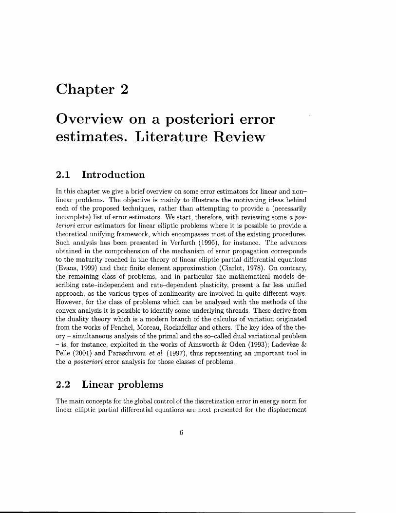
We will consider conforming finite element approximations of the problem(2.1). W ith this regard, let 7^ = {He} be a finite element partition of Q made up of polyhedrons Qe with faces 7 . We denote with £ h,n and £ k'dflt the sets of the faces which are contained in f l (i.e., the interior faces) and in d f l t , respectively. For each face 7 E £ h,ct we denote a fixed unit normal n , chosen arbitrarily from the two possibilities. For the faces 7 E £ h’dci\ n is the outward normal to Q. The definition of the elements f2e,in and f l i t0Ut in relation to n is depicted in Figure 2.1. Let Vq C V

§The symbol : in (2.1) denotes the double contraction operator. W hen it acts between second order tensors it delivers a scalar whereas when it acts between a second order tensor and a vector the outcome is a vector. The symbol ■ is, on the other hand, the inner product between vectors. We also recall th a t the action of a fourth order tensor on a second order tensor is a second order tensor. For the definitions of operations on tensors we refer to G urtin (1981).

7

F ig u re 2.1: Definition of the elements f le,m and i \ out in relation to n

be any conforming finite element space associated with 7^ and {Nf } the basis of the finite element shape functions. The finite element solution G + Vq of the problem (2.1) is given by

Find: u h e u d + Vq

[ C V su h : VrfhdQ = f b • rjh df2 + f t ■ rjh ds V r}h G Vq ^Jn Jn Jdnt

Thus, the discretization error e = u — Uh is solution of the variational problem

Find: e G Vo

/ C(Vse ) : V 77 dfi = / b rj dfl + / t ■ r]ds — / CS7sUh: V 77 dQ, V77 G Vo* / Q J J d$l t */ Q

(2.5)and, one has the error representation formula

lei II2 = / C(Vse): V e d Q = / b-edf i + I t - e d s — I CVsU*: VedQ. (2.6) »/ •/ si J ri

The functional

— / h-77dQ+ / £ - 77ds — / C V .^ : V ^df!, (2.7). / n * / dnt J n

which appears at the right hand side of equation (2.5), is referred to as residual functional of with respect to (2.1). It can be shown that it is an element of the dual topological space* Vq of Vo- From (2.4) and accounting for the definition (2.7) it follows

KuniVh) = [ b-T)h d tt+ [ t - Vhd s - [ C V su h : VTfodfi = 0, Vrjh G V£ (2.8) Jn J dnt J n

* Let V be a topological vector space. The dual topological space V* of V is the vector space of the linear continuous functionals over V. If V is a normed space, a linear continuous functional

v ) over V is a bounded functional, th a t is, sup < 0 0 . In this case, the vector space V* isvev IMIv

endowed with the norm ||.F||v* = sup -jr-Tp - (Brezis, 1986).vev |M |v

that is, the residual functional 7lUh(T]h) vanishes over Vq C Vq. Thus, it is also

(e , rlh)v„ = j CVse : Vr/hd(l = J (&ex - CVsu ^ : Vt}h dfi = 0 , Vrj/, € Vr'‘

(2-9)which is the orthogonality condition between the discretization error e and the finite element space Vq with respect to the inner product defined by (2.2). Condition (2.9) means that the error e E Vo solution of (2.5) presents zero component in the spaceV h vq •

The localization of the integrals in (2.7) over each finite element Qe and use of integration by parts gives

K u d v ) = Y [ r u h r]dn+ [ J uh V ds =ne<=Th 1e£h'dntu£h’n 7

= Y \ [ Y j J 2 h v d s \ . (2 .10)neeTh I Jfle 'yedfie J

In equation (2.10), r Uh = divCVsit/! + b is the regular part of the global residualassociated with the lack of equilibrium of the finite element solution within theinterior of the elements f2e, whereas J 7 has the following definition

77 _Uh[CVsit^: n]^ on 7 G £ h,n

t — CVjW/j : n on 7 E S h,dQt

where [CVaix^: n] denotes the jump of CVsW*: n across the edge 7 E £ h’n \ this value is independent on the choice of n. Thus, J 7 represents the singular part of the global residual due to the lack of equilibrium in the normal tractions across the interelement boundaries and on the boundary dQt, that is, on 7 E £ h'dnt U £ h'n .

Evaluating the discretization error means to solve the same linear elastic model as (2.1) but with different boundary conditions and external loads. Now, the bound­ary conditions are given by e = 0 on dVLd and CVse: n = t — CVsUh'- n on d£lt, whereas the body forces are — divCVgU^ — b over each element £le and [C V5ii/j: n] are the surface loads applied on the faces 7 E £ h,Q.

Nevertheless, problem (2.5) presents the same difficulty as the original problem(2.1), for it is posed in the infinite dimensional space Vo- One could, therefore, think of computing a finite element approximation of e. The adoption of the same finite element space Vq would, however, deliver eh = 0 , because of the orthogonality of e with respect to Vq . If a more accurate approximation for the error e is sought, this would be equivalent to solve the original problem. Furthermore, this would also involve a computational effort that could be directed toward the evaluation of a better approximation for the solution of (2.1). In such a case, however, the error of the new more accurate finite element solution should presumably be estimated in any case, so that the same dilemma re-appears. Keeping at the minimum the

9

computation cost for the assessment of the accuracy of an approximate solution is, indeed, a fundamental feature of any error estimation technique.

The current schemes for accurate and quantitative estimates for the discretiza­tion error are usually classified according to how estimates of a given norm (or linear functional) of e are obtained. Our attention is here mainly directed to the control of the accuracy in energy norm. In particular, we will consider the residual type and the averaging type error estimates.

2.2 .1 R esidu al ty p e error estim ates

The residual functional lZUh(v) is the forcing of the problem (2.5) that defines the finite element error e. As a result, the solution of (2.5) will depend on 1ZUh(v). The starting point for this class of estimators can be assumed to be the equality between the energy norm of the error and the norm of the residual functional in Vq- This follows easily from the definition of norm of residual (see note |) , equation (2.6) and (2.3),

. . . . f C(Vse): V iidfi [ C (V „e): V edfi

l l ^ u J k = »up = sup - — iiMii = - — iiwii = HWH-■ueVo IIMII veVo IIMII IIMII

Estimates for |||e ||| are, therefore, obtained by providing estimates of ||77,uJ|y*. In turn, these can be obtained either through a direct computation using the finite element solution and the available data, or by solving local auxiliary problems, which give a representation of the functional lZUh = 7ZUh(v). The first class of residual error estimates are referred to as explicit whereas the second one is called implicit.

2.2.1.1 E xp lic it residual a poste rio ri e rro r e s tim ates

These estimators were first introduced in Babuska & Rheinboldt (1978b) for the assessment of the accuracy of finite element approximations with higher order ele­ments of ID elliptic problems and then extended to 2D in Babuska & Rheinboldt (1979b). The bound can be expressed, in general, as follows

ll|e ||| < £ { c i M l r u J m n ^ + £ C ^ h l \ \ J l \ \ m x i ^ } (2,11)neeTh 'redQe

where ^ i — 1,2 are interpolation constants (Ciarlet, 1978) which depend on the shape of the element and the local order of the polynomial approximation, whereas he is the diameter of the element Qe.

Apart from the constant all of the quantities on the right-hand side can be computed directly from the finite element approximation and the data for the problem of interest.

The relative importance of the two terms which appear in (2.11), the one associated with the interior residual r Uh and the one associated with the jump

10

were analysed for two-dimensional problems in Babuska & Miller (1987) and in Babuska & Yu (1987) for the case of irregular grids of bilinear quadrilaterals and biquadratic approximations, respectively. In the first case, the dominant term of the estimate was the residual jump whereas in the second case the error could be expressed only in terms of the residual in the interior of each element (see also the work of Carstensen & Verfurth (1999), where it is proven that for general meshes of linear triangles, the energy norm of the error may be estimated by employing only the jump J J J .

Error estimates in norms other than energy norm were analysed in Babuska & Rheinboldt (1981), though for one dimensional problems. However, the theoretical analysis appears quite cumbersome and not providing for an immediate extension. A streamlining of the estimation technique was contributed noteworthily by Johnson and coworkers in Eriksson & Johnson (1991); Johnson &; Hansbo (1992); Eriksson et al. (1995). Their works involve a number of basic ideas which represent also the basis of the estimates for the quantity of interest. The gist of the procedure is the duality argument used by Aubin and Nitsche for the derivation of a priori error estimates in norms other than the energy norm (Ciarlet, 1978). The duality argument is also used for the purpose of deriving a posteriori error estimates through the following points (Johnson, 1994):

1. Error representation formula by means of a dual problem

2. Orthogonality of the Galerkin approximation

3. Interpolation error estimates

4. Strong stability of the dual problem

As an illustration of this procedure, we next sketch the control of the error in L2 norm. Also, for simplicity, we will assume that dQd = dQ. In this case, the error representation formula is given by

[L2(0)] /Jne * e d Q = / CVse: V ^ dfi/Jn

where ip € Vq is solution of the dual problem

CVs v?: V 77 dQ = e • rjdfl V 77 G Vo(2 .12)

As a result of the Galerkin orthogonality (2.9), it is also

CVse : (Vy> — V Tyh<p) dfi (2.13)

11

where l Vh : Vo —> Vq is a suitable Vq-interpolation operator (Clement, 1975; Bernardi & Girault, 1998).

From equation (2.5), the localization of the integral in (2.13) and the use of Cauchy-Schwartz’s inequality, it follows

lle llfL2(n)]3 < ^2 i ll^Jk-C'2 ) ]3!!^ - <Ph\\[mne)}3 +neeTh I

+ ^ 2 HJ nJI[L2(7)]3ll^-^ /i||[L 2(7)]3 •yEdCle

The terms ||(p - ipk\\[L2(ne)]z and ||y? - <Ph\\[L2(dne)]3 describe the weight of the terms llr tiJI[L2(ne)]3 and II JZh\\[L2(dfie)}3 la the local contribution to the error in L2-norm, respectively.

The use of the interpolation error estimates (Ainsworth Sz Oden, 2000)

11 ||[L2(f2e)]3 < C,/e,l||Vv3||[L2(ne)]3x3, Hv?-<^/i||[L2(ane)]3 < C'/e,lllVV?ll[L2(Oe)]3x3’

where Qe is the patch of elements associated with along with the stability of the global dual problem (2.12),

||V y ? ||[L2(n)]3x3 < C'S| |e | | [ L2(fi)]3

where Cs is the stability constant, it finally, gives

He ||[L 2(0)]3 < Cg ^ 2 S C / e )l M * * u J [ L 2 ( f i e ) ] 3 + ^ 2 C ,^ ,2 h e 2 | | ^ u J I [ L 2(7)]3 QeeTh I ~fEdne

The above error estimate does not admit cancellation between different elements Qe and on element level, as well. As a result, it is not very sharp. Furthermore, the mechanism of error propagation is accounted for only through the global stability constant Cs. In order to reflect better the local contribution of the local residual, in the context of control of quantity of interest in linear elasticity, Rannacher & Suttmeier (1997) implement only the steps 1, 2 and 3 of the above procedure. The term || V<£>||[L2(^e)]3x3 is computed numerically by simply taking the first order dif­ference quotient of an approximate solution <ph £ Vq of the dual problem. This procedure was further improved by Suli & Houston (2001) in the case of error con­trol of output of hyperbolic problems. Only the steps 1 and 2 were implemented and an approximation of the dual solution was retained in the bound as a local weight-function.

Given an element Q.e of the mesh 77, the patch of elements associated with f le is the set of elements f li which share an edge with f2e. Given a vertex i of the mesh 77, the patch u>i of elements associated with i is the set of elements fi/ which have i as one of its vertices (Verfurth, 1996).

12

2.2.1.2 Im p lic it residual a p o s te rio ri e rro r e s tim ates

Estimates of the norm of the residual can be also obtained by solving local problems which define approximations to the local representation of the residual as opposite to the explicit estimators described in the previous section, which are computed directly in terms of the norm of the residuals r Uh and . Despite the simplicity of implementation, the main disadvantages of the explicit estimators are the presence of generally unknowns constants and the lack of sharpness of the bound. The latter is consequence of various applications of the Cauchy-Schwartz inequality which provokes the loss of cancellation between the various types of residual (Ainsworth & Oden, 2000).

With the implicit approach, on contrary, in the definition of the estimate, one tries to retain the structure of the equation (2.5), which defines the error, as far as possible.

These estimators have, generally, the following format (Babuska & Strouboulis,2001)

u>i(zTl

where 7Z = {uJi} is a covering of Q and eWi is solution of a boundary value problem of the form

Find: eWi G S(<Ji)(2.14)

CVseWi: VT) dQ = ^ . ( 77), V77 G S(ui)'n

with tS(a>i) a suitable solution space and 1) defined in terms of the residuals

/Jn

Uk 11 'According to the formulation of the auxiliary problems to solve, we distinguish

• subdomain residual error estimators;

• element residual error estimators;

• equilibrated element residual error estimators.

The subdomain residual error estimator was first introduced by Babuska & Rhein­boldt (1978a). The main argument is a localization via a partition of unity of which leads to problems posed on the patch of elements Ui associated with each node i. The solution space S(cJi) is a finite element space with its elements vanish­ing on dtUi — d£lt , continuous and piecewise polynomials of a sufficiently high degree whereas T^Xvi) is given by

^X'n) — / b-r jdQ,+ t r j d s — CVsu h: Vrjdfl.J u>i J du>iC\dnt J u>i

The function eWi is, therefore, solution of a Dirichlet problem with homogeneous essential boundary conditions on dui. Existence and uniqueness of this solution is

13

guaranteed by the Lax-Milgram’s theorem. The local patches used in this techniqueare, however, rather expensive to approximate accurately. In effect, each element is treated several times according to the number of patches with which it is associated. Also, the error indicators ||eWi|| are in this way associated with the patches u>i and not with the single element Qe. This makes more difficult the definition of an optimal adaptive procedure based on ||eWi||. The use of patch of elements Ui is essentially a consequence of imposing Dirichlet boundary conditions on the auxiliary problems and of certain conditions required for the reliability of the error estimator (Verfurth,

On contrary, if only Neumann boundary conditions are imposed on the auxil­iary problems, one can choose u>i = Q,e (Verfurth, 1996). The resulting error estima­tors are referred to as elemental types and an immediate outcome of this approach is to have error indicators defined element by element. However, some care must be taken to insure the local Neumann problems are well posed.

The different estimation techniques differ in the way the well-posedness is achieved. With this regard, we distinguish the equilibrated elemental residual er­ror estimators obtained by choosing the boundary data so that the underlying local problem is well posed and the elemental residual error estimators obtained by choos­

ing the solution space <S(Qe) so that the bilinear form C V ^ : VrjdQ is coercive.

For instance, the second and third version of the error estimates introduced by Bank & Weiser (1985) are of the latter type, whereas the first version is of the former type, which will be described later on.

In the elemental error estimates, the functional J-ne(ri) is given by

where JZh,av is obtained by averaging the jump JZh between the elements sharing the edge 7 E £hfi as follows

In this case, special consideration must be given to the choice of the finite element space <S(fie) in order to guarantee the solvability of the local problems (2.14) and to produce useful error estimators.

In the case of linear finite element approximations of scalar elliptic equations, the space <S(f2e) used by Bank & Weiser (1985) to define the second and third version of their error estimates, is the space of the so-called bubble functions, that is, quadratic functions defined over fle and vanishing at its vertices. This space has been then augmented by cubic bubble functions by Verfurth (1989) in the definition of an error estimator for linear finite element approximations of Stokes equations.

1996).

f b rjdQ+ [ t - T j d C l — f CVsuh: VrjdQ, + f J^hav-r}ds

14

Guidelines for choosing the space <S(Qe) are well established in the case of first order finite element approximations and are discussed in Oden et al. (1989). In the case of higher order finite element approximations, the selection of «S(Qe) is not an easy matter. In general, the criterion is the same as the one underlying the error estimates based on hierarchical bases (Bank &; Smith, 1993): to increase the order of the space used to construct the original finite element approximation and then form the quotient space by subtracting the original finite element space. The influence of the choice of the different spaces on the solution of the local problem has been, however, investigated by Ainsworth (1996). A quite unsatisfactory state of affair has been shown, due to the sensitivity of the estimate to the choice of S(Qe). In some cases the estimator is a gross overestimate, yet in others the estimated error is zero, despite the true error being nonzero. An alternative possibility is given, therefore, by the equilibrated element residual error estimates.

Likewise the estimators described previously, the equilibrated element residual error estimates are obtained by solving local Neumann problems. In this case, the well-posedness of the local problems is achieved by imposing the consistency of the boundary data. The idea is to consider an equilibrated splitting of the interelement flux J£h such that

T7 — T7 .^fi,tn I T'y&l'Out UUh ~ J Uh 1"

f r (2-15) / r„kd n + f J ^ ‘“ds = 0,

and the functional Jrne{ri) giyen by

= [ r Uh ■ 7] dQ + + <f J 2 ? e'in ' V ds.

The second condition in (2.15) is the consistency condition on the data of the fol­lowing local Neumann problem

divCV se^e = r Uh in De

CVse0e: n = on d n e.

which guarantees its well-posedness in [H1 (r^e)]3-Different types of equilibrated element residual error estimates have been given

in literature. These include the techniques proposed by Ladeveze & Leguillon (1983), Kelly (1984), the first version of the error estimate of Bank & Weiser (1985) and the error estimate given in Ainsworth & Oden (1992), among others. These are differentiated between each other, basically, by the assumption on the splitting of the residual jump across the element boundaries.

A unifying theoretical framework for the equilibrated element residual error estimators has been developed by Ainsworth & Oden (1993). The gist of their analysis is a localization of the primal-hybrid variational formulation (Raviart &

15

Thomas, 1977) of the problem (2.5) that characterizes the discretization error. The formulation is posed on the so-called broken Sobolev space Vo(7/l)^ associated with Th and it is obtained by relaxing the interelement continuity with the expense of introducing Lagrangian multipliers /j, = n i y ) E M C V q ^ ) . The latter are the lin­ear and continuous functionals defined over Vo(%) and vanishing over Vo C Vo(%,). The elements of M. permit the characterization of the interelement continuity of elements v E Vo (7^). In this way, one can solve local problems which preserve the type of bound.

The main result is

- 4 l l l e I H 2 = inf sup £ (v ,/i) = sup inf £ (u , / x)> inf' C(v,ti) V)x E M ,2 v€Vo(Th) peM vtVo(Th) veVo(Th)

where is the Lagrangian functional defined as follows

£ { v , n ) = ^ 2 Jne{v) - V* + V

with

J s i S v ) = - f CVsv : V v d Q — j b - v d £ l — f t - v d s +^ Jne Jne Jdnennt

+ / C V su h : Vv dQ + (b g da e • v d sJ Q e J d f l e

a n d

^ ( V) = / * 0 7 - M 7 ds- (2‘16)7efh.n 7

In equation (2.16), g 1 is a smooth vector field associated with each 7 E £h,si and [u]7 is the jump of v E Vo (7^) across 7 (see note ft). The particular choice of g7 determines the error estimation method. Once g7 has been chosen, the vector field gone is defined on d£le for each element f le e T ^ such that

y * 0 9dde • v d s = V grn- JdCl* J-y

7 L j ] 7 d s .neeTh Jdn* 7e£h,n

By choosing /x = /x*, one obtains

nflr* *'eVo<n,)

^ T h e broken Sobolev space Vo(%,) is the space of the functions v of class [H1 (Oe ) ] 3 over each element Q.e G 7^ which meet homogeneous essential boundary conditions on df l e D As aresult, an element v € Vo(%.) may be discontinuous across 7 € £h,n- We define [u]7 = lim u (x +

q|0an) — lim u (x — an). If we let Vo(Be) = j u € [H1 (Oe)]3|v = 0 on df l e D j , it is Vo{Th) =

1 1 Vo(fle).gT/i

16

where Vo(f2e) is the restriction of Vo (Th) to Qe (see note ff).The inequality (2.17) gives the link of the error estimate 77 to the solution of

the following elemental primal problems

Find w 6 V0(ne)

uev0(ne)(2.18)

The complementary principle applied to the solution of (2.2.1.2) delivers

Find p E Wne

Gne(p) = supgeWn,gewne * Jne

q . q dQ

Gne(q)

where W ne is the set of the stress tensors q solution of the following problem over

that is, a concrete realization of an upper bound for depends on the definition °f 9ane and on the choice of q 6 Wne •

The equilibration of the data (2.19), which is necessary for the model problem under consideration, is desirable to realize also when low order terms are present in the elliptic operator. In this case as the mesh size h —> 0, these terms can become preponderant and make the energy of the local solution blowing up. By imposing the equilibration of the data also in this case, the error estimator becomes finite (Ainsworth & Oden, 2000).

The error estimator introduced in Ladeveze & Leguillon (1983) can be casted into the previous framework by choosing gdne to be JZh,av P us a suitable piecewise linear vector field on dQe (Verfurth, 1999). However, this error estimate has been obtained by starting from other considerations which lead to the class of errors in

Q 'ri = gne, on d\le.This set is not empty if the following condition is satisfied

(2.19)

which is the equilibration condition. Since it is

\ V L ^ e{v )= sup gne(q)we Vo (He) q€W{ie

then it follows

e| | |2 < - 2 ^ SUP Gcie( q ) < ~ 2 Gne(q) V g e W n e,n ee r h

17

the constitutive equations and they will be considered next. The previous analysis provides also theoretical support to the heuristic error estimate introduced by Kelly (1984) consisting in the solution of local complementary problems.

Finally, it is worth mentioning that Paraschivoiu et al. (1997) have devel­oped an extension of this theory to the estimates of output of interest. Besides the relaxation of the interelement continuity, an additional constraint is introduced represented by the equilibrium equations over the broken Sobolev space, so that the admissible set is constituted by the only solution of the problem (Patera & Peraire, 2001). The value of this generalization lies in the application to problems which can be expressed in terms of minimization of a convex functional. An instance of such extension to a hyperelastic model has been given in Bonet et al (2002).

The error in the constitutive equation. The Prager-Synge theoremThe notion of error in the constitutive equations has been introduced for the first time by Ladeveze in 1975 (Ladeveze, 1975; Ladeveze, 1995) by exploiting the convex functional structure of the constitutive equations.

For linear elastic problems, this notion can be grasped quite easily. Let crex = crex(x ) and u ex = u ex{x ) be the exact stress field and the exact displacement field, respectively. This means that crex does satisfy the equilibrium equations, u ex is a kinematically admissible displacement field, that is, u ex meets the internal and external compatibility conditions and finally, u ex and a ex are related to each other by the constitutive equation

<Tex ~ c V su ex = 0. (2.20)

Consider now a kinematically admissible displacement field u ad = u ad(x). The energy norm of the error associated with u ad = u ad{x) is defined as

\\\Uad ~ UexlW = ^ I l^ex - C V sU ad\: C_1 [<Tex - CV sU ad] dfi^ (2.21)

Upper bound for (2.21) is obtained as

v ( u ad, (Tad) = ( ^ J Wad ~ CVsu ad] : C_1[cr ad - C V su ad] (2.22)

where crad = crad(x) is any statically admissible stress field, that is, a stress tensor field that satisfies the equilibrium equation. As a result, crad meets also the condition

I (aex - (Tad): (V su ex - V su ad)dQ = 0, (2.23)Jn

which follows, by standard arguments, from the principle of the virtual work.Equation (2.22) is a measure of the extent to which the pair (a ad, u ad) fail to

satisfy the constitutive equation (2.20) and is obtained by reformulating equation

18

(2.20) into an equivalent form which uses the convex free elastic potential and its Legendre transform, given by the complementary potential.

The validity of the bound

Given u ad(2.24)

111 &ex I I I ^ ^ i ^ a d t ^ a d ) ■> ^ & ad

is a simple consequence of the Prager-Synge’s theorem (Prager & Synge, 1947) which states the orthogonality between the fields crex — CV su ad and crad — crex. This reads as

/Jn'Q

= I icr

\(Tad G V s ^ a d ] • G [ ^ a d dfl —

I \crex - CV su ad] : C_1 [crex - CV su ad] dQ + (2.25)Jn

T I \(Ta d GValter] . C [ ^ a d CVsliex] dfi.J n

Proof. In the case of linear elasticity, by accounting for the equivalence

1 1<Te x C(V jW e x ) 0 ~CTex . C & e x "T ~ s ^ e x • G V s Z L e x ( T e x . V s ^ e x — 0

it is an easy matter to show the validity of the following equality

2 0 " a d • G ( T a d T ^ ^ s ^ a d • CV s ^ a d O’a d . V sUad —

= ~ (T ad ■ G (Tad T 2 ^ s'U'ex • C V s U ex O’ad . V s^ e x T

+ -<r„: C -1<xeI + - V 3ua,,: CV„uad- a ex: V su ad +

(o"ex (Tad) ■ ( ^ s'U'ex ^s^ad) i (2.26)

so that by integrating both sides of equation (2.26) and accounting for (2.23), equa­tion (2.25) follows. □

In the case of conforming finite element displacement approximations, one assumes u ad = Uh so that the actual realization of an upper bound rj for the energy norm of the error |||e ex||| resolves in the definition of a statically admissible stress field crad. However, for the efficiency of r) the definition of crad must be linked with the finite element solution crh = CV sUh- This is realized with the so-called prolongation condition introduced by Ladeveze & Leguillon (1983) which is a localization at each element of the Galerkin orthogonality (2.9) which holds for the global residual 7£U/i. This condition distinguishes the statically admissible stress fields crad which satisfy the following equation for every shape function N* and for all the elements Qg,

J (crad - C V su h^ : VNi dft = 0.

19

This condition, finally, corresponds to making an assumption on the splitting of the residual jump across the interelement boundaries and crad is obtained as solution of the following local problem stated for each element fle

div crad + b = 0

where J ^ e is the part of the jump across 7 G dQ,e which is assigned to Qe. Error indicators are obtained simply by the localization of the integral (2.22)

as

where

JfleThe proof of (2.24) has large validity so that the error in the constitutive

equations has also been applied to 2D and 3D elasticity by Ladeveze et al. (1991) and Coorevits et al. (1998), respectively; incompressible elasticity by Gastine et al.(1992) and to anisotropic meshes in Ladeveze (1994) and Ladeveze & Rougeot (1997). In each of these problems, the crunch of the estimation technique was always the definition of the equilibrating element tractions recovered by the finite element solution. A general procedure for such construction in the case of 2 D finite element models has been developed in Ladeveze Sz Maunder (1996).

As we have mentioned earlier, local equilibrium problems with repartition of the residual jump have been proposed on heuristic basis also by Kelly (1984). It can be noted that the repartition that Kelly assumes in ID corresponds to the prolongation condition introduced in Ladeveze & Leguillon (1983).

The concept of using two approximate solutions to build estimates of the error had been put forward also by Synge (1957) in establishing the hypercicle method. By using two approximate solutions located in spaces intersecting at the exact solution Synge builds estimates of solutions of the torsion problem.

We conclude this section by mentioning the work of Fraeijs de Veubeke (1965) that can be cast within the previous framework. Fraeijs de Veubeke provides esti­mates of the energy norm of the exact solution | | |u ei||| starting from the two-sided bounds for the exact free elastic energy in terms of the total elastic energy and the total complementary elastic energy. Let

be the total elastic energy defined over the afRne space of the kinematically admis­sible displacement fields and

20

the total complementary elastic energy defined over the affine space of the statically admissible stress fields. It is (Mikhlin, 1964)

Vltacj, 3 \ u ad) ^ 3 i^ex) Qi&ex) ^ Qi^ad)i ^&ad-N--------V-------- '

1112 2 III 111

Thus, estimates of the energy norm of the exact solution | | |u ei||| were obtained as

l { u ad, (Tad) = y/-2g((Tad) + 2 J ( u ad)

This procedure, however, failed to gain popularity being based on the global solution of the dual finite element method for the model under consideration, and also because the estimate cannot be expressed in terms of the contributions from each element, necessary for the optimization of the finite element meshes.

2.2.2 R ecovery based error estim ators

The recovery based error estimators represent certainly the class of error estimates that has met a big success in the engineering community for its relatively simple implementation. They were first introduced by Zienkiewicz h Zhu (1987) and since then many error estimators have been developed which employ the main idea. This relies on the following fact. The energy norm of the error, given by equation (2.3), can also be re-written as follows

e = (^ J {(Tex - c v su h) : C 1(crex - CVsu h) dQ^ , (2.27)

where the exact stress field crex is unknown. Therefore, estimates to |||e ||| are obtained by assuming in place of a ex in (2.27) approximations cr* recovered by suitable postprocessing of the finite element solution crh = CVgU^, that is

llle lll ~ V = {^J {cr* - CVsu h) : C 1 (cr* - CVsu h) d o j .

The quality and reliability of this type of error estimator is however dependent on the accuracy of the recovered solution. In general, it can be said that if cr* is such that

f (crex - a *): C-1 (crex - a*) d f l < f (cr* - C V su h) : C-1 (a* - C V su h) dfl »/ n >/ n

then

[ ( a * - C V su h) : C~1 (cr*—CV su h) dfl « f (crex- C V su k): C-1 (aex- C V su h) dfi. Jn Jnand one can define

n = ( J (o-* - CVsttft): C-'fo-* - CV.u*) d fi)

21

as an a posteriori error estimator (with respect to the energy norm).The procedures to build a* are, generally, referred to as the stress recovery

or derivative recovery techniques. The definition of these methods finds their mo­tivation in the observation that, under some conditions on the domain, mesh and regularity of the solution, there exist certain points of the domain where the deriva­tives of the finite element solution, CV aUh, which are usually one order lower than that of the finite element solution itself u^, have superior accuracy (Barlow,. 1976). This phenomenon is known as superconvergence. If super convergent derivatives can be recovered by a particular post-processing method, an asymptotically exact error estimator is then obtained (Ainsworth k Oden, 2000).

The recovery technique given initially in Zienkiewicz k Zhu (1987) assumes cr* interpolated by the same functions as the displacements, i.e.

cr* = No-* (2.28)

where cr* are the nodal values of the continuous field cr*. These are obtained by im­posing that cr* — CV sUh is orthogonal to the space described by the shape functions N, that is,

j (cr* — CV sUh) : N dQ = 0.J n

The Zienkiewicz-Zhu (Z 2) error estimator, whose corresponding error indica­tors are obtained simply by localization of the integral, was analysed in Ainsworth et al. (1989). It was found that while the estimator performs quite well for linear triangular and quadratic quadrilateral elements, it is not necessarily asymptotically exact. This property is shown to hold in the case of smooth solutions and parallel meshes by Babuska & Rodriguez (1993) and in Verfurth (1996) who refer to the analysis carried out by Rodriguez (1994). For other types of elements, the Z 2- method was often found to behave poorly with the effectivity index converging to zero in some cases. In others, the error indicators were misleading in steering the dis­cretization process (Strouboulis k Haque, 1992). For this reason, Zhu k Zienkiewicz (1990) introduced first for one dimensional problems a new stress recovery proce­dure, termed as super convergent patch recovery, by means of which superconvergent derivatives of the finite element solution are determined everywhere in the domain. The recovery procedure was then developed for 2D problems in Zienkiewicz k Zhu (1992a) and applied to error estimation in Zienkiewicz k Zhu (1992b). The contin­uous stress field cr* is, as usual, assumed to be given by equation (2.28). The nodal values <r* are obtained by considering a continuous polynomial expansion on an el­ement patch surrounding the nodes where the recovery is desired. This expansion is made to fit locally the superconvergent points, called also sampling points, in a least-squares manner or simply be an L2-projection of the finite element deriva­tives. For the least-squares fitting, the superconvergent recovery is observed by the numerical test; for the local L2-projection fitting, a considerable improvement for the nodal values is achieved.

Improvements of the method were contributed by Wiberg k Abdulwahab(1993) that include the governing equilibrium equation on the recovered derivatives.

22

As in Zienkiewicz &; Zhu (1992a), these are assumed to be interpolated by the same shape functions as the finite element displacement field, that is, cr* is assumed of the form (2.28). The nodal values of the recovered stress field are also here obtained by assuming for the stresses a polynomial expansion over the patch of elements around the given node. The coefficients of this expansion are then computed by minimizing, in a least-square sense, the residual of the stresses at the superconvergent points and the weighted residual in the equilibrium equation over the local patch of elements. This recovery techniques was successively improved by Wiberg et al. (1994) for the recovery of derivatives near the boundaries where either tractions or displacements are prescribed. This was obtained by including seemingly a weighted residual error at the boundary points in the patch recovery and a pronounced improvement in the post processed gradients of the finite element solution was finally observed.

A complete analysis of the several recovery based error estimators in terms of the operator that defines the improved stress as function of the consistent derivatives of the finite element solution can be found in Ainsworth & Oden (2000). Carstensen &; Funken (2000) analyze, on the other hand, their robustness with respect to vio­lated (local) symmetry of meshes or superconvergence and with respect to incom­pressible locking.

These error estimators, however, are justified to varying extent by supercon­vergence properties which are known to hold only in special cases. In Babuska & Strouboulis (2001), therefore, a new definition of superconvergence - the 77%- superconvergence - is considered which generalizes the classical idea of superconver­gence to general meshes. By means of this property one can choose the best position of the sampling points when properties of superconvergence do not hold.R em ark 2 .1 . If the smoothed stress field cr* is chosen as an equilibrated stress field a ad, for instance, with the criteria given in the previous section, then one retrieves the equilibrated element residual error estimates. □

A numerical methodology which determines the quality of a posteriori error estimators has been set up by Babuska et al. (1994b) and Babuska et al. (1994a). The authors observe that the use of general benchmarks to validate a posteriori error estimates can lead to wrong conclusions if they are not properly chosen to isolate the basic factors which influence the performance of the estimator. As a result, an objective and standardized means to assess the robustness of an estimator that exercises all the feature of the particular estimator is given. However, this methodology presents its own limitations. The procedure allows the evaluation of the extreme bounds of the effectivity indices for the estimator when certain effects such as the influence of the singularities, the effect due to the boundary of the domain and mesh grading have been isolated. Moreover, the effectivity indices are those that would be obtained in the asymptotic limit when the mesh size approaches to zero. The preasymptotic behaviour of the estimators might well lead to rather different conclusions concerning the suitability of a particular estimator. Thus, this methodology must be seen not as a means to justify an estimator, but rather as a minimal criterion the estimator must meet. For the details of the procedure and its motivating ideas we refer to the above works and to Ainsworth & Oden (2000).

23

The main general conclusions of the studies carried out in Babuska et al. (1994b) and Babuska et al. (1994a) on the quality of estimators for piecewise affine finite approximations on triangular elements can be summarized as follows

• The performance of an estimator depends on the class of meshes, solutions and materials of interest.

• Among the residual estimators tested by the above authors, the implicit el­ement residual estimator with equilibration was the most robust, namely it gives good results for several mesh types, for highly orthotropic materials and arbitrary grid material orientations. In particular, the equilibration proposed in Ladeveze & Leguillon (1983) was recommended.

• The Superconvergence patch recovery error estimator developed in Zienkiewicz k, Zhu (1992b) gives good results for the class of smooth solutions approxi­mated on patchwise uniform grids of linear and quadratic elements.

• Asymptotic exactness for an estimator can occur for special uniform grids only and cannot give a measure of quality for the estimator for the general meshes employed in engineering computations.

• The quality of the analysed error estimators tends to deteriorate on anisotropic meshes.

The value of the methodology lies also in the fact that it requires only the solution of small problems in the region of interest; it is inexpensive and it can be used to check the quality of any new estimator even if it is only available as a black-box computer subroutine.

2.3 Nonlinear problemsUnlike the linear problems analysed in the previous section, where a certain maturity has been reached in the comprehension of the mechanisms of propagation of the error, in the case of nonlinear problems, and in particular for those dependent also on the time, the theory of error estimation can be considered still in its infancy. This is reflected in the paucity of studies dedicated to the m atter and of originality of the approaches, which usually try to adapt ideas developed for linear problems. Although it is difficult to make a classification of the techniques of estimation, for the nonlinearities are involved in a quite different ways and for the different nature in the approximation of the time and space variable, it may be useful to distinguish the several contributions as follows (Gallimard, 1994):

• Error estimators for problems where the time variable does not appear;

• Error estimators which attempt to estimate also the effects of the time dis­cretization;

24

• Error in the constitutive equations;

• Methods based on heuristic considerations and direct to the development of error indicators.

For each of this class, the more meaningful works will be outlined, especially in relation to plasticity.

2.3.1 N on linear increm ental problem

An approach to a theoretically justified a posteriori error estimate for the finite element approximation of plasticity problems was given in Johnson & Hansbo (1992). These authors analysed the regularized version of the Hencky problem in small strain perfect plasticity with Von Mises yield criterion given by

where and a^ denote the solutions of the regularized problem. In equation (2.29)p represents the regularization parameter, whereas P is the projection operator on the yield surface defined by

well-posed in the usual Sobolev spaces (Duvaut h Lions, 1976). For the original model of perfect plasticity, on contrary, the displacements must be sought in the more technical space of the bounded deformations (Temam, 1985) if one requires to guarantee their existence.

Let the complementary energy norm of the error on the stresses be defined as

linear operator P is called a projection if P 2 = P. If P is a projection, then ||P x || < ||a;|| Vx G V, thus (x , (I — P)x) > 0, i.e. I — P is monotone (Brezis, 1986).

div (Ttl = b

u fl = 0 on dfi,

in O

(2.29)

if llrD H > av(2.30)

where ay is a material constant and t d = r — |T r[r] J is the deviator tensor of r . Equation (2.29) describes also the physical model of viscoplasticity which is

where denotes the consistent finite element stress tensor obtained from the dis- placement finite element approximation of (2.29). From the monotony of the oper­ator I — it follows

V n - r f W e < ^ ( e )

^Let V be a Hilbert space. An operator A : V —> V is called monotone if (x , Ax) > 0 Vx G V. A

25

where e = — u^h and the functional (77) is the residual produced by cr* inthe equilibrium equations, which is given by

- [ <rh \ V 77 df2.J n

Further to a heuristic argument, Johnson & Hansbo (1992) distinguish two contributions into One contribution comes from the part Q,el of the domain0 which remains elastic both in the continuous and in the finite element model, whereas the other contribution comes from the complementary part Qpl = Cl — Qel. As a result, they finally propose the following estimate

k - < t £ i i e < ( f y h c i R ^ w\ j = 1

where

= iVh = div <r£ + 6 on Qe G Th

R2{cTu) = max sup --------------------------- on Qe G Th7C9f2e 2i ft= M : n h on 7 G s h'n

CS = | |V sl tM||[Ll(n)]3x3 4- | |V sUMi/l||[Ll(n)]3X3

and Cj are the usual interpolation constants.The two contributions to the error estimate in (2.31) reflect the type of de­

pendence on the mesh size present in the a priori error estimate found by Johnson (1976b) for finite element approximation of this problem. Therein, the estimate has the following structure

||crM “ ^ W e < 0{h) + 0 (V h )

with the 0(h) and 0(y/h)-terms related to Qel and Q,pl, respectively. However, since the a priori error estimate is sub-optimal, one expects the mesh will be more refined in the plastic part Qpl, where the stresses are suspected to be rather smooth (Fuchs k Seregin, 2000).

Furthermore, the estimate (2.31) is not a full a posteriori error estimate, since Qel and Cs depend on Therefore, the authors suggest to replace with u^h for the computation of Cs and assume for f2eZ only the part of the discrete model which remains elastic. This is quite arbitrary, for it implies that the plastification zone is already correctly captured on the current mesh.

The analysis of the Hencky problem in small strain perfect plasticity with Von Mises yield criterion has been considered also by Rannacher k Suttmeier (1998). As a special case of the control of output of interest, they obtain an a posteriori error estimate of the energy norm of the error on the stresses via duality argument applied

L2(fiel) + Cs J (2.31).7 = 1 /

Kr i fa ) = I b-r jdQJQ

26

to a linearized dual problem. Starting from the non-linear variational equations which describe the regularized version of the Hencky problem and its corresponding finite element approximation, they obtain the non-linear Galerkin orthogonality relation

where the mean integral theorem has been invoked and P ' is the tangent stiffness matrix sampled at V (suM+ (l —s)u^h) with s e]0,1[. By computing the linearization (2.32) at u^h, they consider the solution of the following linear dual problem

in the case of control of the error in energy norm. Following standard arguments, finally, they obtain

whereas the weights are approximated as in the linear case.Since this estimation technique involves a linearization, the resulting estimate

will be valid only asymptotically, that is for close to u lJL. Moreover, one is required to provide an approximation for e in order to define the forcing J s i v ) in the dual problem, which can provoke a deterioration of the quality of the bound.

Duality has also been employed to derive a posteriori error estimates for non­linear variational problems. The work of Repin Sz Xanthis (1996) represents an important1 contribution in this sense. The authors, indeed, develop a rigorous math­ematical analysis based on duality theory of the calculus of variations which leads to the concept of duality error estimators for approximations to nonlinear problems defined by a special class of convex functionals. In particular, the theory is presented for the Nadai deformation theory (Nadai, 1937) of hardening elasto-plastic material

P (C V su M) - P (C V su ^ ) : Vrfadfl = (2.32)

Find </? e V

f f P ' ( V u ^ h)Vrj\ V<pdQds = J(r j) Vry Jo Jn

where J (77) is the output functional of interest which is taken equal to

with the local residuals defined by

Pne = ^ne|lr ^ll[L2(oe)]3 + h^e ^ | |J j J [ L 2(ane)]3'yCdfle

27

which gives rise to two variational problems: the primal for displacements and the dual for the stresses,

Vr G E£q, Q(t ) <Q{(Tex) = sup Q(t ) = J { u ) = inf J ( v ) < J { v ) , Vv e Vtezeq

where J (v ) corresponds to the potential energy of the elasto-plastic body defined over the affine space V of the kinematically admissible displacement fields and Q{r) corresponds to the complementary energy of the elasto-plastic body defined over the affine space Eeq of the statically admissible stress tensor fields. For the definition of the functionals J { v ) and Q(r) associated with the material model under consid­eration we refer to Repin &; Xanthis (1996). Likewise Fraeijs de Veubeke (1965), Repin & Xanthis (1996) assume the difference £(v , t ) = J ( v ) — Q{r) as measure of the energy norm of the approximation error. However, due to the computational cost and difficulty for building equilibrated stress fields r the functional£(v , t ) is extended over the whole space E of the stress tensors. As a result, Repin & Xanthis (1996) obtain the following estimate

^\\\v - u | | | 2 < £(v , t ) = £ \ ( v , t ) + £eq(r).

For the expressions of £a (v , r ) and £eq we refer again to Repin & Xanthis (1996). Here, in relation to further developments we note that the analysis of Repin & Xanthis (1996) shows that £a (v , t ) = 0 if and only if the constitutive equation is satisfied, whereas £eq(T ) = 0 if and only if r satisfies the equilibrium equations. For this reason, £a (v , t ) measures the error in the constitutive law and £eq{T) measures the error in the equilibrium equations. The estimate, which is an extension of the one proposed by Ladeveze h Leguillon (1983) for linear problems, can, therefore, be applied by using the known approximate solution v of the primal problem and the corresponding stress tensor obtained by the constitutive relation, even though this will not meet the equilibrium equations. However, the actual computation of the estimate, which is developed for any conforming approximation, not necessarily meeting an orthogonality condition, requires the solution of a quadratic minimiza­tion problem posed over an infinite dimensional which renders its practical applica­tion rather difficult. Furthermore, the estimate does not distinguish the elemental contributions, which form the basis of any adaptive process.

An a posteriori error estimate for the primal variational formulation of elasto- plasticity with linear hardening given in Han & Reddy (1999) is provided by Al- berty et al. (1999). The a posteriori error estimate refers to the finite element approximation of displacement and plastic strain field in the nonlinear incremental boundary value problem obtained within one time step of the backward Euler. With this formulation, the continuous formulation and finite element discretization of the nonlinear incremental boundary value problem can equivalently be expressed as min­imization of a Lipschitz-continuous non-smooth convex functionals. By exploiting this property Alberty et al. (1999) obtain the following estimate

II47 ~ + lleP ~ e£llfi,2(n)]3><3 + l|Vstx - Vs«fc||fL2(n)]3x3 < C ^ ^ e,neeTh

28

where C is a constant depending on the hardening modulus, the discrete stress field a h is

a h = C(Vsu h - el),

whereas the elemental error indicators 77 are given by

vhe ~ ^nJl’Vllfi,2 )]3 + 2 ^711 11 \ l2 (7)]3icdne

which are the same as in pure elasticity. This circumstance is motivated by the observation that the evolution law in the plastic material law (within one time step) is satisfied exactly on each element whence the material law has a vanishing residual. Thus, excluding the error accumulation for progressing time-steps, the only remaining residuals are those produced in the discrete equilibrium conditions.

2.3 .2 A n alysis o f th e tim e d iscretiza tion error

The error estimates presented in the previous section, though based on solid theoret­ical background, by definition do not account for the effects of time discretization. These estimates, indeed, have been developed by looking at the error associated with the finite element approximation of the non-linear incremental boundary value problem obtained from a one-time step discretization of the initial boundary value problem. Therefore, the error estimate cannot take into account the error deriving from the replacement of the rate quantities appearing in the initial boundary value problem with the difference quotients. It is, indeed, this replacement that produces an error, called the time discretization error, which in certain cases may not be negligible.

An inherent difficulty in obtaining a complete a posteriori error estimation for the solution of the fully discrete scheme is due to the different nature of discretiza­tion: finite difference-type in time and finite element-type in space. With a finite element approximation-type, the error can be linked to the residual associated with the approximation. This is obtained simply by inserting the approximate solution into the exact equation. With a finite difference approximation-type, on the other hand, it seems impossible to insert the discrete solution into the exact equation and compute the residual. In this case, indeed, the error estimates developed for finite difference approximations of ordinary differential equations are traditionally based on predictor-corrector algorithms. In these algorithms the difference in solutions obtained by schemes with different orders of truncation error is used as rough esti­mates of the error. This estimate is in turn used to adjust the time step (Gear, 1971; Reiher, 1987; Abbo & Sloan, 1996). An alternative is the estimate proposed by No- chetto et al. (2000) that develop a posteriori error estimates for the backward Euler approximations of a special class of abstract evolution equations in Hilbert space. In their method it is the accuracy of time interpolant functions of the nodal values, such as continuous piecewise linear or discontinuous piecewise constant functions, to be assessed.

29

This unsatisfactory state of affair, however, does already become clear in the development of a posteriori error estimates for parabolic equations which represent the simplest class of evolution problems. For this reason, it seems appropriate to first recall briefly some works for parabolic problems. This is considered useful in relation to the evolution of elastoplastic systems.

Eriksson & Johnson (1991) develop an adaptive algorithm for the heat equation based on a posteriori error estimates of approximations obtained by the discontinu­ous Galerkin method which is based on space-time discretization. In the context of the error analysis, one of the advantages of using the discontinuous Galerkin method is the availability of a unique global variational structure which provides directly the approximation in space and in time. In this manner, one can represent the error in terms of the residual produced by the approximation in the global variational formulation of the problem which will, therefore, account for the discretization ef­fects in space and time (Estep et al, 2000). The use then of a space-time duality argument allows one to realize the control of the quantity of interest. The main idea of this technique, which extends to time dependent problems the procedure developed for elliptic problems, can be comprehended by considering the following abstract evolution equation in the Hilbert space 7i (Nochetto et al, 2000)

Find u : t G [0, T] —> 7i

u + F{u) = 0 (2.33)

u(t = 0 ) = u0

where T : Tt —► TL is a given (nonlinear) operator of TL in TL. Let 71 be the residual

7l = - U - T { U ) , (2.34)

where U is the approximate solution. By adding (2.33) and (2.34), we obtain the error equation for e = u — U

e + Ue = 7l (2.35)

whereu def f VJ F ( s u + ( l - s ) [ / ) d s .

JoMultiplying (2.35) by tp G Cl (^,T]\TL) and integrating by parts over [0,T] delivers the error representation formula

T r T(e,(fi — U*(p)dt + / {1Z,(p)dt (2.36)

Jowhere U* is the transpose of U. The a posteriori error estimate follows then byselecting ip in (2.36) as the solution of the backward dual problem

Find (p(t) : t G [0,T] —> TL

— U*(p = 0

V(T) = e(T)

<e(T),V(T)) = {e( 0 ) ^ ( 0 ) ) + /Jo

30

and using strong stability properties of </?, such as bound for ip, for evaluating the initial error and the residual terms.

The implementation of these ideas to the discontinuous Galerkin finite ele­ment method dG(0)cG(l), which combines continuous piecewise linear polynomial approximation in space with discontinuous piecewise constant polynomial approxi­mation in time (which then reduces to the backward Euler with the rectangle rule applied to the integrals) delivers the estimate (Eriksson et al., 1996)

| u(tN) - UN ||L2(Q) < L NCi ^ a x ^ (\\h2nR 2{U)\\In + \\h2nf l +

(2.37)

+ | | [ ^ n —l ] | |L 2 ( 0 ) + | | f c n / | | / „ + || - r H ^ n - l l l l ^ O )rCrj.

where

M k = max ||* ||l2(0 ),t n - \ S t S t n

u(tN) = u(9 ,tN),

Ci and L n are constants depending on kn = tn — £n_i and tn,

1 l|[Vt/]||iJ(7)= max su p ----- — ,

’ 7 2 hnHg E 7ftn, with the finite element partition Thn associated with In = [£n_i, tn\}

hn meshsize of 7^n,

and the starred term is different from zero only in presence of change between non­embedded finite element meshes. In equation (2.37) one can distinguish the terms that measure the residual error of the space discretization from those that measure the residual error of the time discretization. Among the latter, we consider further the starred term. This can be interpreted as error of the initial data of the single one step problem due to different interpolation assumption: in presence of non­embedded finite element spaces, V/ln_ 1 <£. Vhn, the L 2 projection of Un -1 E Vhn_x onto Vhn is different from £/n_i.

Phase change phenomena represent a class of problems interesting to consider for they share some common features with the evolution of an elastoplastic medium, such as the presence of variational equations and differential inclusions in the gov­erning equations. In the problem studied by Chen et al. (2000b), for example, we have

Find 0, x

( f t ,r,) + ( ^ , v ) + ( V 0 , V v ) = ( f , v ) , V!}

where e is a small scalar parameter, 6 stands for the temperature of a substance that occupies the domain Q and undergoes solidification, x is the phase variable and A

31

is a multivalued operator given by the inverse of the sign function. The primary variables 9 and x are approximated with continuous piecewise linear finite elements in space and the backward Euler method is employed for the time discretization.

In the error analysis carried out by the same authors, time interpolation func­tions of the nodal values of x and 9, and also the constant interpolant function 0(0 = 0n, with £n_i < t < tn are employed in the definition of the error. Starting from a representation of this error, the authors finally derive an estimate which is expressed as sum of several contributions. These include the term associated with the jump residual, the internal residual, the coarsening, the initial error, the time residual, the quadrature and the error on the data.

The extension of the previous procedures to the control of the error in the dis­placement formulation of an elastoplastic continuum is not straightforward. This is due mainly to two reasons. One is the high nonlinearity involved in the elastoplastic behaviour while the other is the use of primary variables, such as displacements, which do not appear in rate form in the formulation of the problem. Consequently, studies on the global control of the error are rare in the current literature. Rannacher h Suttmeier (1999) present a fairly complete analysis for the mixed-dual formulation of the quasi-static Prandtl-Reuss model defined by the following equations

(<r — C V sv, cr — r ) > 0, Vr E IIW

where V = (u E [L2(Q)]3 : v = 0 on and IIW = { r E W : | | r D|| — ay <0 , a.e. in Q}, with W = [L2(f2)]3x3.

After performing time discretization with the backward Euler method, and the introduction of the nonlinear operator P defined in (2.30), problem (2.38) is transformed into the nonlinear variational equation

Data: (<rn_i,w n_i) E W x V

Find: (crn, u n) E VV x V

( Vi P\cTn— l T knC.Vs('U/n ^n-l)], ") W kn((Tn) ^ P) (^n, tp ) ,

V ( r ^ ) E W x V .

Equation (2.39) describes a material behaviour of Hencky-type in the case kn = 1, crn- \ = 0 and u n_i = 0 which is discretized with standard finite elements in space as follows

Find: cr E IIW, v = u E V

(<r, Vtp) = (b,(p), V VE V (2.38)

(2.39)

Data: (<Tn-i>u n-i) e W h x Vh

Find: ( a ^ u hn) e W h x V h

(o-£ - P[<r£_! + knC V s(u^ - ujj.i)], r h) + kn{ a ^ V<ph) = (6 n, <ph)

V(Th,<ph) E W h x V h.

(2.40)

32

For the control of the global stress error with respect to the energy norm, He^Hf; = {ea ,Q~lea) ) in order to account for effects of time and space discretization Ran- nacher & Suttmeier (1999) consider the split of the total error into the three com­ponents

V ( t n ) - < * n = - ° ’n + ? ’n ~ & n + ? n ~ (2‘41)Cn,ff gjj

where

• cr(t) is the exact solution of problem (2.40),

• crn is the solution of problem (2.39) with data crn- i and wn_i,

• a n is again solution of problem (2.39) with data and u^l_1

• cr% is solution of problem (2.40),

thus

• en>(T is the error produced by time discretization only,

• enjCr is the error due to change of data in the solution of (2.39),

• is the error produced by space discretization only.

While for Rannacher & Suttmeier (1999) provide an a posteriori estimate which is the same as for the discretization error of the Hencky problem, for the other two terms only a rough a priori estimate is given. In particular, for e„iff the following bound is obtained

max ||en J | e < ||e° ||jb+ T1 max {kn max ||cr0<n<JV +l a l<n<A T+l te[ tn, tn+ 1 ] J

which shows that the error due to the incremental loading process grows at most linearly with time provided that the exact solution stayed bounded. As for the error enj<T related to the use of inexact starting values in each incremental loading step, this depends on the stability properties of problem (2.39). Rannacher & Suttmeier (1999) give the following estimate

i < ^ +i ^ t 11

which assumes an unchanged propagation of the full size of the error of the data.The error estimate is finally obtained by combining all the previous results.

Nevertheless, the adaptive algorithm given in Rannacher & Suttmeier (1999) is based only on the estimate of the term e£ ff, for the effects of time discretization are neglected.

The same authors set up also a theoretical framework for a posteriori error analysis for the time discretization error based on duality. To this end, the solution of (2.40) is seen as arising from the use of a space-time approximation which uses

33

discontinuous Galerkin method dG(0) for the time discretization and standard finite element for the discretization in space. Further to a space-time duality argument on the linearized equation that defines the error the following estimate is obtained

N + l 4

\\<r(T) ~<Tn +i \\e < +n = 1 fi?GTfcn i = l

where the local residuals are given by

Pn! = hnlkn* f ll-Ri||[La(ne)]3>df, p ^ = h ^ k ~5 f \ \ r h\\[L2h)]3dt,J t n - l J t n - 1 j c d d ™

Pn! = h^\kn~2 [ \\rah\\[L2 {ne)]zdt, p%* = ||[L2(ne)]3*3 ,J t n - 1

withR , d4 f ffO + 1 (0 -'* - P a " ) - V .«„,

A*whereas the respective weights are obtained by the solution of the linear continuous dual problem. Here, it is interesting to note that the term reflects the low order regularity of the time constant piecewise function due to the presence of the discontinuity jump across the time instant tn.

A similar approach has also been adopted by Larsson et al. (2001) for the control of quantity of interest in the space-time discretization of viscoplasticity. Also here, the latter is realized with space-time finite elements that are based on the use of the discontinuous Galerkin method for the time discretization and standard finite elements for the space discretization. This formulation gives quite naturally the variational setting for the analysis of the global error. Consequently, the general principles of duality given at the beginning of this Section can be applied.

Both the theoretical analysis of Rannacher h Suttmeier (1999) and the study of Larsson et al. (2001) share the same limits. These are inherent to the technique of error estimation based on duality when it is applied to nonlinear problems. One limit comes from the need of linearization of the problem that defines the error, so that the eventual estimate has only an asymptotic character. Another one comes from the need of solving exactly the continuous dual problem. Finally, the lack of a sufficiently developed theory of problems of elasto-plasticity does not allow a complete regularity study, which is very important in the analysis of the weights. All this hampers the practical use of the method.

R em ark 2 .2 . The discontinuous Galerkin method dG(0) applied to time discretiza­tion is the backward Euler method with (•)“ = (•)+ and the rectangle rule applied to the integrals. This method, however, does not accommodate the case of using different starting values, that is, (•)“ ^ (•)«• On other hand, the use of the discontinuous Galerkin method dG (l) in place of dG(0), though it has (• )“ ^ (•)+, would produce a different time scheme different from the backward Euler. □

34

Following an heuristic argument baaed on the comparison of the Prandtl-Reuss elastoplasticity with Hencky’s plasticity, Barthold et al. (1997, 1998) split the total error into spatial and time discretization errors. The error associated with space discretization is captured by three terms. The first term is related to the lack of equilibrium and likewise in the work of Johnson & Hansbo (1992) this term is given by

rleq= { ^ i^ l l^ l lfL ^ n e )]3 + C2h2 H ^ llf i,^ )]3}'yCdQe

with C\ and C2 interpolation constants. The second term is due to the violation of the consistency condition at points of the domain other than the Gauss points, as a result of the interpolation of the variables. This term has been introduced in Barthold et al. (1996) and is given by

iKT — IIA/(<X> a ) ~ OTi)||L2(n) = ||A/l/(<T/l, Of/i)||z,2(fl)

where / ( c r ^ ,^ ) denotes the yield function sampled at (c r^ ,^ ) with ah being the kinematic-internal variable and the plastic multiplier, which are both obtained from the finite element computation. Finally, the last term is the error in the plastic dissipation given by

rlL = \W' (ep -e £ ) ||£ 2(n) + | |H a ( d - d k ) | | |2(fi)

where H is the hardening modulus.The time discretization error, on the other hand, is due to the numerical

integration of the flow rule. The error produced within the time interval [tn, tn+1] is defined as

v i t — ll^n+ O lltL ^pxa II f epdt — Aep||[L2(n)]3X3 (2.42)J t n

where the weight ||cr(tn+1)||[L2(0 )]3x3 has been added by Barthold et al. (1997) in order to be unit consistent with the space discretization error. Further to plausible assumptions, (2.42) is estimated by the maximal change of the normal (with respect to the yield function) between two time (load) steps. It is indeed this result to be interpreted physically as measure of the deviation of Prandtl-Reuss plasticity from Hencky plasticity in the current time step.

However, the aforementioned error measure appears to rely more on heuris­tic considerations motivated by the physics of the phenomenon which is not met, rather than arising from a theoretical argument typical of an error analysis. Fur­thermore, the computation of the several terms is realized by assuming recovered post-processed solutions in place of the unknown exact values. As a result, the estimation technique lends itself to the same type of criticism as for the recovery based error estimators.

A family of error measures with clear physical meaning and capable to account in a simple manner for effects of time and space discretization is represented on the other hand by the error in the constitutive equations, which is the objective of the next section.

35

2.3 .3 Error in th e C on stitu tive E quations

The error in the constitutive equations which has been applied successfully for the assessment of the accuracy of conforming approximations to linear problems is ex­tended in a natural way to nonlinear dissipative problems of evolution.

Fundamental notion of this class of error measures is the definition of the so- called admissible solution. This is a particular approximate solution of the given initial boundary value problem. Its definition depends on the conditions and equa­tions which are satisfied, whereas its quality is assessed in terms of the conditions and equations that are not. The application, then, of this theory to assess the quality of a finite element solution consists in building a corresponding admissible solution that reflects the approximations associated with the finite element solution.

The first error measure which exploits these concepts is the one based on the Drucker’s inequality (Drucker, 1964). The definition of this error is due to Ladeveze (1985) in the context of the nonincremental method LATIN applied to the solution of the evolution of elastoviscoplastic materials which follow the conditions of Drucker’s stability. This error measure was then further investigated in Coffignal (1987) and applied in Ladeveze et al. (1986) to the control of incremental finite element solutions of the same class of problems.

The error in the constitutive equations based on Drucker’s inequality applies to material models defined by the following functional constitutive equations

In particular, the material model is supposed to obey to the Drucker’s inequality. This property of the model can be formulated as follows (Bussy Sz Remond, 1985; Ladeveze & Pelle, 2001). Consider any pair of stress-strain history ( c r ( £ ) ; e ( r ) , r < t) and (or(t)-,e(r),T < t) which meet Vi € [0,T] the constitutive equation (2.43) and the initial conditions, which are assumed equal to zero. The constitutive model defined by the operator A is called stable according to Drucker if the following condition is satisfied

whereas it is strictly stable if also the following additional condition is met

The error in the constitutive equations based on Drucker’s inequality assesses the quality of admissible solutions Sad — (<jad, *w) which are defined by assuming

cr{t) = *4(e(r), r < t) (2.43)

where A denotes the constitutive operator which is function of the strain history!.

V(<r,e), (<7 , e) meeting equation (2.43)

(2.44)

W e [ ° , T1], [ c r ( r ) - <t ( t ) ] : [ e ( r ) - e ( r ) ] d r = 0 =* 5 (2.45)cr = cr

^Recall th a t the restriction of the function / ( r ) to times r not later than the current tim e t is called the history of / up to the tim e t.

36

at any time instant t € [0, T], a kinematically admissible displacement field u ad and a statically admissible stress field <rad. Both u ad and crad are required to meet the initial conditions at t = 0. As a result, Sad is an approximate solution to the initial boundary value problem, for the constitutive equations (2.43) are generally not satisfied. The quality of Sad is characterized by defining first the following two processes meeting the constitutive equation (2.43)

S = (A { V su ad(T,T < t))\ead(r, r < t)"--------------v-------------- '

& ( t )

S = { c T a d i t^ A ^ i c T a d iT , T < t ) )

€(r,t<t)

where A ~ l denotes the inverse operator of A, and then computing the following quantity

' D r u c k e r (T) = sup [ [ [<t(t) - (Tad{r) \ : [cad(r) - e(r)] d r dQ > 0. (2.46)t< T Jo Jo

ri2(x,t)

Indeed, by means of equations (2.44) and (2.45), one can easily check that eDrucker meets the following properties

& D r u c k e r ^ 0

& D r u c k e r — 0

O’ — (J ad

C — €adV x e f i , V £e[o,T ],

that is, eDrucker can be assumed as measure of the extent to which Sad fails to satisfy the constitutive equations, and therefore of the extent to which S ad fails to coincide with Sex, the exact solution of the problem. Elaborating on the expression of r)2( x , t ) in the case of material models described by internal variables, Ladeveze & Pelle (2001) show that rj2( x , t ) can be expressed as sum of the error in the state law and the error in the evolution law,

1- O’): c ‘ (cr - it) + ( X - X ) : (V - y )]

+ 22 JoTdr

where X denotes the set of kinematic-type internal variables, Y are the respec­tive thermodynamic conjugate variable and T > 0 is related to the residual in the evolution law. Without further details related to the definition of these quantities which will be analysed in Section 3.5.1 .2 , here, we want just to observe that this decomposition is consistent with the fact that Sad does not satisfy the complete constitutive equations. A similar structure of the error will be noted also in the extended dissipation error introduced in Ladeveze et al. (1999) for material models with internal variables which admit a standard formulation (Halphen & Nguyen,

37

1975). For this new measure of error, the admissibility conditions include the kine­matic compatibility relations, the equilibrium equations and the initial conditions. As a result, the only equations left apart are the complete constitutive equations, i.e. the state laws and the evolution laws.

The error measure (2.46) has a global character in time and space. Further­more, due to its definition, it is not possible to distinguish the contribution to the error arising from time and space discretization, thus it cannot be used to drive an adaptive process. To remedy this, Gallimard (1994) and Gallimard et al. (1996) have applied the concept of error in the constitutive equations to the problems ob­tained by using only time and space discretization, respectively. In this way, the authors have obtained error indicators that separate the effects of time and space discretization, respectively, which then have been used to control the discretization process.

The first use of the error in the constitutive equations to constitutive models described in terms of internal variables and having an associative flow rule is due to Ladeveze (1989). The admissibility conditions combine the kinematic compatibility relations, the equilibrium equations, the state law and the initial conditions. The only equation which is left out is the evolution law that governs the dissipative phenomenon. By exploiting the convexity structure of these equations, Ladeveze (1989) introduces, therefore, the concept of dissipation error given by the residual in the evolution law, which is appropriately reformulated in terms of the dissipation pseudo-potential and its Legendre-Fenchel transform. The theory of this error will be detailed in Section 3.5.1.1.

Likewise the error measure based on Drucker’s inequality, the dissipation error has then applied in Moes (1996) and Ladeveze &; Moes (1997) to assess the accu­racy of incremental finite element solutions of associative problems. Furthermore, error indicators which separate the sources of the different discretizations have been defined and used to drive the adaptive process in time and space.

As we have already mentioned, another measure of the error in the constitu­tive equations has been introduced in Ladeveze et al. (1999) for material models described by internal variable and admitting standard formulation. The new mea­sure is an extension of the dissipation error obtained by removing the state laws from the admissibility conditions. Applications of this error measure have been given for an elastic-damage coupled model in Ladeveze et al. (1999) solved with the nonincremental LATIN method and to the Prandtl-Reuss plasticity model in Orlando & Peric (2000) solved with the classical incremental finite element method. The extended dissipation error will be detailed in Section 3.5.1.2 and will represent the tool employed to analyse the effects of change of finite element mesh in classical finite element incremental solution of elasto-plastic problems.

The measures of the error in the constitutive equations given in this section apply to associative material models. Their key property is the characterization of the constitutive equations as solution of a scalar equation defined by convex scalar potentials. If the equation is not satisfied, it assumes positive value. This same characterization of the constitutive equations has also been given by de Saxce

38

(1992) to a much larger class of materials, such as the non-associated model of cyclic-plasticity of Chaboque-Marquis and the non-associated model of Drucker- Prager, which are termed implicit standard models. The characterization is based on the introduction of a unique potential, function of the rates and the associated force, which is used by Ladeveze (1999) to extend the notion of dissipation error also to this class of material models, whereas applications of the new measure of error have been given in Hjiaj (1994).

2.3 .4 H euristic Error Indicators

Lately, the emergence of new supercomputer architectures has allowed large-scale simulations of engineering problems and the incorporation of more detailed physics in the model. This has led to a substantial increase in the complexity of the simulation process that also incorporates non-linear mathematical models. As a result, adaptive strategies for the approximate solution of these problems are often based on heuristic error indicators or adaption indicators. A physically based argument is generally adopted as justification of their definition, which is typical for the problem under consideration. The motivation in using error indicators is that their primary quality is to be able to distinguish the elements and time steps which contribute mostly to the global accuracy of the approximation, even though they finally may fail to yield accurate global estimates. As a result, they represent a tool for the adaptive construction of the approximation, that is, they may be used as a guide for a sequence of discrete choices (to refine or not to refine a given element; to reduce or not to reduce a given time step) and not for the definition of the stopping criterion which should be based on an error estimate. It also appears clear that works in this area are much more abundant than in that of the development of error estimate. In the following we give only a brief overview of some error indicators that have been employed in practice.

The recovery based error estimate introduced by Zienkiewicz & Zhu (1987) has been applied in Zienkiewicz et al. (1988) to assess the finite element approximation of the flow formulation of incompressible plastic flow in which elastic effects are neglected. The above authors observe that in extrusion problems the energy norm has a definite meaning as it is simply the error in the rate of energy dissipation. Consequently, the total energy dissipation norm is defined as

Since the basic formulation is mixed and the pressure variable is introduced as a means of ensuring incompressibility, Zienkiewicz et al. (1988) consider the energy

where u is the displacement field, and the error e = u — as

39

norm of the deviatoric part of <r, whose constitutive equation is

. D H De

where D is an appropriate material tensor and ^ is the viscosity which in general is dependent on the strain rate.

As a result, the energy norm of the error is written as

e = / (<r° - a h'D) : (^D )-1 (<td - <rh'D) dfiJ S l

(2.47)

The estimate of the measure of the error defined by equation (2.47) is obtained by replacing the exact solution erD with an approximation crD'* of higher order to that given by the finite element solution and obtained with the recovery technique described in Zienkiewicz & Zhu (1987).

This error indicator by its definition accounts for only effects of space dis­cretization. It is thus used as basis for the refinement of the finite element mesh in the current time step. Furthermore, it does not account for the error in the incom­pressibility condition, which is enforced in a weak sense in the mixed formulation.

A posteriori error estimates based on the Zienkiewicz-Zhu adaptive strategy and the energy norm have been appropriately modified by Peric et al. (1994) to ac­count for the elastoplastic deformation of the conventional and Cosserat continuum model. The corresponding error estimates are based on the rate of plastic work and on the plastic dissipation. After introducing the following definitions of error,

Cyyp —

ex?

^ 2 f \(tr — <7h ) : ( e p — € ^ ) |\ f- /"T" J f2e

dnL neeTh

(2.48)

£ [ | (er — <rh) : (ep — epk) + ( X — X h) : ( a — 6lh) \, ^ J a.

dnfleETh

where a denote the set of kinematic-type internal variables and X the respective conjugate thermodynamics forces, estimates for (2.48)i and (2.48)2 are obtained by simply replacing the exact values with postprocessed solutions of the finite element approximation. The error based on the dissipation functional, in particular, has been then employed as basis for the finite element adaptive solution of a strain localization problem. The latter has been described by resorting to the Cosserat continuum in order to overcome serious limitations exhibited by classical continuous models in the post instability region. The expression of the estimate has been particularized for the classical model of J 2- elastoplasticity which is generalized by introducing additional degrees of freedom within the Cosserat continua. In this case it is shown that the expression of the plastic dissipation involves only classical quantities. Assuming time discretization of the evolution problem is performed by the backward Euler

40

algorithm, within a generic time step In = [tn, £n+i], the a posteriori error estimate €z> based on the dissipation functional is given by the following expression

ep = ] T£le£Th

« + l o P (n+1

R.n+ln+1

^ + i) +

'n+1 ^ a n+l ^ a n+l dff

where P is a second order tensor used to represent the yield function in the seven­dimensional stress space for plane strain J 2-elastoplasticity within a Cosserat con­tinuum, whereas a denotes the accumulated plastic strain and R the conjugate variable. The starred quantities denote the postprocessed solutions. Likewise the previous error estimate, error indicators are simply obtained by localization of the integrals at each element. These error indicators are, in turn, used only to drive mesh refinement, for they reflect only effects of space discretization.

A comparative evaluation of various error estimators for isotropic, elasto­plastic and viscoplastic solids undergoing large deformations has been carried out in Tetambe et al. (1995). Five distinct error estimators are studied. These are the L 2 -norm of the stress error,

h = JJn(cr — crh) : (cr — crh) dfl

h =

the L2-norm of the total strain error,

[ (e - e h): (e - eh) dfl

the L2-norm of the equivalent total strain error,

[ (teq-teq)2^Jfl

h =

where eeq is an equivalent scalar strain given by an appropriate norm of the total strain e; the L2-norm of the incremental total strain given by

h = [ (Ae - A eh) : (Ae - Ae*) dfiJn

and finally the energy rate error norm introduced by Zienkiewicz et al. (1988). As usual, estimates for these measures of error are obtained by simply replacing the ex­act values with approximations of higher order, obtained by a suitable postprocessing of the finite element approximation. This study shows that the error computed using

41

each of these estimators increases from its initial value as the deformation continues in the plastic zone in a large strain analysis. In particular, the error estimators based 011 the energy rate and the L2-norm of the incremental strain were able to predict the region with the maximum error.

Since these error estimators are defined in terms of incremental quantities, they mirror to different extent the effects of only space discretization. As a result, they are not able to predict consistently a monotonically increasing error with the deformation.

The adaptive procedures for large-deformation finite element analysis of elastic and elasto-plastic problems implemented by Lee & Bathe (1994) is based on a pointwise indicator for error in stresses and a pointwise indicator error in plastic strain increments. The pointwise error in stress indicator is a pointwise version of the stress smoothing type of indicators. This indicator estimates the error in the stresses by giving the differences between the unaveraged stress a h and a smoothed stress <t*. In particular, only the pressure and the effective stress (which are related to the first and second stress invariant) are considered in the evaluation of the accuracy of the finite element solution. The error in the plastic strain increment tensor is given by

Ae eP = Aep - A eph (2.49)

wherertn+l

A ep = / epdt.J tn

An estimate of the error (2.49) is computed by considering the L2-norm of the difference between the plastic strain increments obtained using the trapezoidal rule, which is second order accurate, and the Euler backward method. Though this is an indicator on the time discretization error, it is used in Lee & Bathe (1994) as indicator of the space discretization error along with the indicator for the error on the stresses.

In the context of adaptive strategies for problems with localization of defor­mations Ortiz & Quigley (1991) argue heuristically that localized solutions may reasonably expect to be of bounded variation. The total variation of the solution over each element is thus assumed as a suitable adaptor indicator to drive the adap­tive process. For ID problems, the bounded variation of a scalar function v = v(x) is defined as follows

Given: v : [a, b\ C M —► M(2.50)

MBV,[a,b) = SUP EfcLl M x k) - v(Zfc-i)|

where the supremum is taken over all sequences a = x 0 < x\ < . . . < xn = b, VN £ N. Elements are targeted for refinement when the variation of the solution within each element is determined to be too high for the interpolation to adequately resolve it. Ortiz & Quigley (1991) also show that in ID problems this error indicator

42

can be derived from interpolation error bounds, that is, the equidistribution of the indicator (2.50) over the mesh is shown to minimize the L°° interpolation error.

Use of error indicators based on minimization of interpolation error have also been employed by Demkowicz et al. (1985) and Radovitzky & Ortiz (1999), among others. In these works, the methodology set by Diaz et al. (1983) for grid optimiza­tion, that is, for relocation of the nodes within a fixed number of degree of freedom, is employed for mesh refinement. The estimation of the local errors is based on interpolation error bounds and extraction formulas for highly accurate estimates of the derivatives of the exact solution which appear in the bound. In the method­ology proposed by Radovitzky & Ortiz (1999), starting with a very fine mesh, the discretization error can be bounded from above by the interpolation error, once a linearised analysis is carried out. In order to compute the size of the exact solution, which appears in the a priori error bound, Radovitzky & Ortiz (1999) consider the error of a lower order approximation p 1 1 such that the computed finite element approximation p ph represents the finite element nodal interpolation of p ^ 1.

These error indicators are based on a priori error estimates, therefore, usually, they deliver crude estimates. However, they present the advantage since they can be applied for those problems where energy estimates based on the residual break down due to the loss of ellipticity of the governing equation. Therefore, they must be used with judgement, for they imply a certain regularity of the exact solution and require accurate techniques to calculate derivatives of the exact solution.

2.4 Concluding remarksThe considerations of the previous sections show that the formal structure of the theory of a posteriori error estimation for linear problems is well understood, as opposite to the non linear problems. This mirrors the different maturity achieved in the theoretical analysis of the two classes of problems.

In the class of the linear elliptic problems, the recovery based error estimators represent perhaps the most widely used a posteriori estimates in solid mechanics applications for its relatively simple implementation. Also the explicit residual type error estimates are quite easy to use, for they simply require computing norms of the residual, once a certain weight between the jump term and the internal residual has been set. However, the way that the residual influences the error is accounted for by the stability properties of the dual problem, whose solution can pose further difficulties. The implicit residual type estimation of the error, on contrary, deliver much more effective estimates at the fraction of cost of solving additional local finite element problems posed on local higher order finite element spaces. In this class, the error in the constitutive equations developed by Ladeveze &; Leguillon (1983) appears to be the most robust.

For nonlinear problems, very few theoretically based error estimates have been developed. In particular, for time dependent problems, the measures of the error in the constitutive equations have clear physical meaning and are able to account

43

for all the sources of discretization. In the finite element solution of elastoplastic problems discretized in time with the backward Euler method, which will be the class of problems hereafter considered, apart from time and space discretization, another source of error needs to be considered. This arises as a result of the change of finite element mesh from one time step to the other, which introduces a discontinuity jump in the time linear interpolation of the discrete values of the solution. As a result, only measures of error that account for time discretization effects can reflect the low order regularity of the approximation across the time tn when the change of mesh occurs. Thus, the extended dissipation error introduced by Ladeveze et al. (1999) naturally lends itself for this aim.

The theoretical analysis of this measure of error and the way it is able to accommodate discontinuity jump in the admissible solution is the main objective of the next Chapter.

44

Chapter 3

The error in the constitutive equations for dissipative nonlinear problems

3.1 IntroductionIn this chapter the general theory to assess the quality of the so called admissible solutions of dissipative nonlinear problems is presented following Ladeveze h Pelle (2001).

After introducing the set of conditions and equations that govern the behaviour of a standard generalized model with internal variables (Halphen & Nguyen, 1975), and noting the dissipative nature of the elastoplastic problem under examination, a simple error analysis of the following first order ordinary differential equation

u'{t) + a(t)u{t) = /(£),

u(t — 0) — u0

with a > 0, is performed. This is done in order to motivate the use of residual of approximate solutions of dissipative problems as indication of the error produced and also to show the influence on the error of the discontinuity jump which is present in the approximate solution at the time instant tn. An a posteriori error estimation analysis is given, which delivers an upper bound expressed in terms of the discontinuity jump.

As introduction to the error in the constitutive equations, the fundamental no­tion of admissible solution is given. This is a particular approximate solution of the problem under exam. Its definition depends on the conditions and equations which are satisfied, whereas its quality is assessed in terms of the conditions and equations that are not. Consequently, the concepts of dissipation error and extended dissipa­tion error for time continuous admissible solutions, and the one with discontinuity jump at the time instant tn are given. A new measure of error in the constitutive equations of rate-independent plasticity models is defined which is called augmented

45

extended dissipation error. Finally, a definition of error in solution concludes the chapter.

3.2 The reference continuum problem: The Ini­tial Boundary Value Problem for a model with internal variables

3.2 .1 P relim inaries

Consider a generic continuum body B with boundary dB occupying a regular domain Q of the three dimensional Euclidean space. Let dBd and dBt be disjoint parts of dB, with dBdUdBt = dB, where displacements and surface tractions are prescribed, respectively. We will assume displacements to be small in the quasi-static evolutive process of the body so that geometry changes and inertial effects may be neglected. As a result, the analysis will be performed in the reference configuration which is identified with the domain Q while the boundary dB is identified with <9fL Likewise, the identifications dBt with and dBd with dVLd are assumed, as well.

3.2 .2 E quilibrium E quation

Denote with S the linear space of the symmetric second order stress tensors. The statically admissible stress fields, <r = er{x, t ) G S, are such that the weak form of the equilibrium, given by the virtual work, is satisfied, that is,

f cr: Vr/dQ = f b ■ rjdQ,+ f t ■ 77ds V77 G Vo, V£ G X = [0, T] (3.1) Jn Jn Jdfit

where b = b(x, t ) and t = t{ x , t ) are respectively the body force and surface traction fields and Vo is the linear space of the virtual displacements which vanish on dQdi whereas X is the time interval of interest (Gurtin, 1972; Ladeveze, 1999). Whenever necessary, the equilibrium condition will also be written as

{a{x, t ), Vrj{x)) = (b(x, t), rj{x)) + {t{x, t) ,r j(x))dni,

with (•, •) and (•, *)ant denoting integrals over the domain Q and the boundary d£lt where traction conditions have been assigned, respectively.

3.2 .3 C om p atib ility E quations

The compatibility equations refer to the displacements and the associated defor­mation. The conditions which define a kinematically admissible displacement field guarantee internal and external compatibility. In mathematical terms, this means that a displacement field u = u (x , t ) is kinematically admissible if it is time con­tinuous, at least once differentiable in space and meets the boundary conditions on

46

dQd- We refer to V as the space of the kinematically admissible displacements.Let 8 be the linear space of the symmetric second order strain tensors. The kine­matically admissible strain fields, e = e(x ,t) € 8 , are continuous fields which are obtained from the kinematically admissible displacement fields u = u (x , £) € V as follows

e = h v u + VtiT) = V ,u , (3.2)z

i.e., e is the symmetric part of the second order tensor V u.

3 .2 .4 C on stitu tive E quations

3.2.4.1 Therm odynam ic A dm issibility

In the constitutive modelling with internal variables, which is hereafter adopted, the functional dependence of the present state of the material upon the history of the total strain and temperature (which are the observable variables) is replaced by equations that define the current state of the material in terms of only the current value of both the observable variables and additional variables, called generally hid­den or internal variables. They are macroscopic measures of irreversible phenomena (Lemaitre & Chaboche, 1990; Besson et al., 2001). The success of such formulation is due to the simplicity, in general, of the mathematical and numerical analysis of the problem which governs finally the evolution of the whole system.

Our interest, in particular, will focus on constitutive models of rate inde­pendent plasticity in isothermal conditions belonging to the class of the so-called standard generalised materials as introduced by Halphen & Nguyen (1975). By ex­ploiting the convex structure of these models, emphasis will be placed especially on scalar equivalent formulations of the tensorial constitutive equations.

The physical validity of a constitutive model is usually expressed by its thermo­dynamic admissibility (Coleman & Gurtin, 1967; Maugin, 1992), which is obtained by imposing the validity of the Clausius-Duhem inequality. For isothermal processes, the aforementioned inequality represents the difference between the external total power and the rate of variation of the reversible stored energy, that is,

—ip + cr: e > 0, (3.3)

where ip is the free Helmholtz energy per unit volume defined in terms of the state variables which describe the model, and cr: e is the total external power.

The inequality (3.3) is obtained by combining the local form of the first princi­ple of thermodynamics, which expresses the conservation of energy, and the second principle, which refers notably to the direction of irreversible processes.

A thermodynamically consistent model is, therefore, obtained by specifying the state variables along with the functional form of the free Helmholtz energy and the complementary laws which describe the time evolution of the internal variables in respect of (3.3).

47

3.2.4.2 State variables

In the definition of the state variables, which characterise uniquely the state ofthe system, we refer only to the so called kinematic type variables whereas thecorresponding static one are obtained by duality as introduced by the total energy and the dissipation. In particular, we assume the following: (i) temperature to be constant with time and uniform in space so that it will not be considered hereafter; (ii) that the total strain can be uniquely decomposed additively into its elastic and plastic part, that is,

e = ee + ep, (3.4)

and finally (iii) that the local state of the material is described by means of ad­ditional internal variables a which may only include scalar and/or second order tensors (Coleman & Gurtin, 1967; Reddy & Martin, 1994), characterizing the inter­nal changes of the material.

3.2.4.3 Equations of State

The reversible energy density stored under any form in the material is represented by the free Helmholtz energy -0 which is assumed to depend on the variables (ee, a) . In particular, we assume to be expressed as a sum of two proper strictly

CTy

e(t) £

F igu re 3.1: Energy repartition for a linear elastic and linear isotropic hardening model

convex and lower semicontinuous functions of each of its arguments: ipe{^e) which is the stored energy due to elastic strain and ^ p{ol) which is the stored energy due to plastic and internal parameters related to hardening effects (Nguyen, 2000), cf. Figure 3.1, i.e.,

^(ee,a ) = ^e(ee) + ^P(«)-

By expanding the Clausius-Duhem inequality which is required to hold for any admissible thermodynamic process (e,ep,a ) (Coleman h Gurtin, 1967), we obtain the state equations

d'ljje t 4 d'lpp

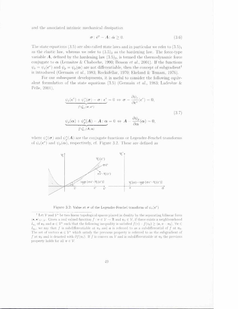
and the associated intrinsic mechanical dissipation

cr: ep — A: cx > 0. (3.6)

The state equations (3.5) are also called state laws and in particular we refer to (3.5) i as the elastic law, whereas we refer to (3.5)2 as the hardening law. The force-type variable A, defined by the hardening law (3.5)2, is termed the thermodynamic force conjugate to a (Lemaitre & Chaboche, 1990; Besson et al., 2001). If the functions

= ^ ( e 6) and = fyp(a ) are not differentiable, then the concept of subgradient^ is introduced (Germain et al, 1983; Rockafellar, 1970; Ekeland & Temam, 1976).

For our subsequent developments, it is useful to consider the following equiv­alent formulation of the state equations (3.5) (Germain et al., 1983; Ladeveze Sz Pelle, 2001),

A ( e e) + VCM - er: ee = 0 <b> a - ^ ( e e) = 0, v ' dee

3elllltl{fT\ee)(3.7)

i>p(a) + - A : a = 0 o A - = 0,V ^ ✓ O C X.

pVl , t (A ' a )

where 'ip*{cr) and 'ipp(A) are the conjugate functions or Legendre-Fenchel transforms of ^ ( e 6) and ipp(a) , respectively, cf. Figure 3.2. These are defined as

F igu re 3.2: Value at cr of the Legendre-Fenchel transform of ijje{ec)

t Let V and V* be two linear topological spaces placed in duality by the separating bilinear form (•, * )v \v - Given a real valued function / : n G V —> R and no £ V, if there exists a neighbourhood /„0 of Vo and a G V* such th a t the following inequality is satisfied f (v) — /(no) > (a , v — no), Vn G

we say th a t / is subdifferentiable at no and a is referred to as a subdifferential of / a t no- The set of vectors a G V* which satisfy the previous property is referred to as the subgradient of / at vq and is denoted with d / ( n 0). If / is convex on V and is subdifferentiable at no the previous property holds for all n G V.

49

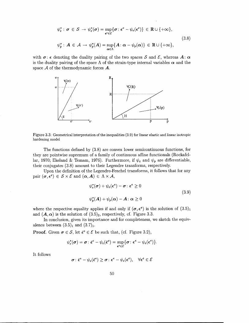
V£ : cr £ S —► ipl(cr) = sup{<r: €e - ^ ( e 6)} G M U {+ 0 0 },«ee£

(3.8)'ip* : A £ A i/>p(A) = sup{A: a - Vt>(°0} ^ {+ 0 0 },

aGA

with cr: e denoting the duality pairing of the two spaces S and £, whereas A: a is the duality pairing of the space A of the strain-type internal variables a and the space A of the thermodynamic forces A.

P P

a

a

F igu re 3.3: Geometrical interpretation of the inequalities (3.9) for linear elastic and linear isotropic hardening model

The functions defined by (3.8) are convex lower semicontinuous functions, for they are pointwise supremum of a family of continuous affine functionals (Rockafel­lar, 1970; Ekeland & Temam, 1976). Furthermore, if ipe and V>p are differentiable, their conjugates (3.8) amount to their Legendre transforms, respectively.

Upon the definition of the Legendre-Fenchel transforms, it follows that for any pair (<r, ce) £ S x S and (a , A) £ A x A,

'ipl(a) + ipe(€e) ~cr: ee > 0(3.9)

V£(A) + V'p(a) ~ A : ol> 0

where the respective equality applies if and only if (<7 , ee) is the solution of (3.5)i and (A , a ) is the solution of (3 .5 )2 , respectively, cf. Figure 3.3.

In conclusion, given its importance and for completeness, we sketch the equiv­alence between (3.5) 1 and (3.7) 1 .

Proof. Given cr £ S, let ee £ S be such that, (cf. Figure 3.2),

ip*e{cr) = cr: ee - V>e(ee) = sup {cr: ee - V'efc6)}-eees

It followscr : i e — 'ij’eic6) > cr : ee — Vee £ E

50

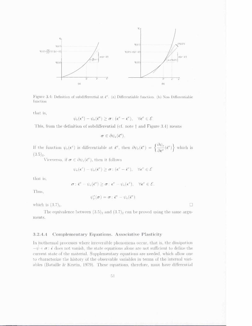
Vt (£ ')

>l't(e’)+t^(E*)[e,- e ’]

£ ' E*(b)

F igu re 3.4: Definition of subdifferential at ee. (a) Differentiable function, (b) Non Differentiable function

that is,^ e ( e e) - ^ ( e 6) > cr : (ee - i e), Vee G £

This, from the definition of subdifferential (cf. note f and Figure 3.4) means

cr G <9t/>e (e e).

dipIf the function i)e(ee) is differentiable at €e, then d ^ e{ee) = |-^ -^ (e e) j which is (3.5)!.

Viceversa, if cr G d ^ e(e e), then it follows

that is,

Thus,

^e(ee) - ^e(€e) > cr: (ee - ee), Vee G £

c r : ee - t/;e(ee) > cr : ee — t/»e(ee), Vee G £ .

ip*e{a) = cr : ee - ^ e{ee)

which is (3.7) i. □

The equivalence between (3.5)2 and (3.7)2 can be proved using the same argu­ments.

3.2.4.4 C om plem en tary E quations. A ssociative P la s tic ity

In isothermal processes where irreversible phenomena occur, that is, the dissipation —ip + cr : e does not vanish, the state equations alone are not sufficient to define the current state of the material. Supplementary equations are needed, which allow one to characterize the history of the observable variables in terms of the internal vari­ables (Bataille & Kestin, 1979). These equations, therefore, must have differential

51

character, that is, they have to relate the rate of the internal variables to the asso­ciated thermodynamic forces. The conjugacy is here meant in the sense of power as defined by the intrinsic mechanical dissipation cr \ ep — A: a which is used to relate by duality the space E = E x A of the rate of internal variables (ep, —at) with the space E = S x A of the thermodynamic forces (cr, A). Here, we have denoted with S the linear space of the rate of the strain tensors ep, and with A the linear space of the tensorial quantities represented by d .

The complementary equations are only restricted to meet the intrinsic mechan­ical inequality (3.6). Since cr: ep — A: at represents the part of the plastic power which is actually dissipated in heat form, assuming the non negativity of the intrin­sic mechanical dissipation means that we require the irreversible processes described by the constitutive model under consideration to produce heat (Besson et al., 2001).

There are several approaches to the definition of the complementary laws in the respect of (3.6) (Chaboche, 1996). A simple way to ensure a priori the thermo­dynamic consistency of the model is given by the class of the standard generalised materials introduced in Halphen & Nguyen (1975). In this model, one assumes the existence of a potential of dissipation tp(ep, — d ) in the space E = E x A of rate of dissipative variables, which is positive, convex in its variables and such that tp(0, 0) = 0. The complementary laws are then given by

(cr, A) e dip(ep, —at) (3.10)

where the symbol d denotes the subdifferential operator (Rockafellar, 1970; Ekeland &; Temam, 1976). As a result of the properties of tp(ep, — at) and the definition (3.10) of the complementary laws, the thermodynamic consistency of the material model follows quite easily:

Proof. From the meaning of sub differential of a convex function, and the duality established by the mechanical intrinsic dissipation, it follows

tp(ep', — at') — tp(ep, —at) > cr: (ep — ep) — A: (at' — a ) , V(ep , —at') E E.

Thus, for (ep/, —a ') = (0,0) one obtains

tp(0 , 0 ) — tp(ep, —d ) > —cr: ep + A : at

and for the properties of cp(ep, —at), it follows finally

cr \ ep — A : cl > tp(ep, — d ) > 0

□The definition of the complementary laws (3.10) in terms of the subdifferen­

tial allows the important class of non differentiable dissipation potentials associated with time independent dissipative processes, which is hereafter considered, such as dry friction, plasticity, brittle fracture and damage, to be included in the same the­oretical framework (Panagiotopoulos, 1985; Nguyen, 1994). The rate independent

52

phenomena, in fact, are characterised by assuming the dissipation potential as a lower semicontinuous convex positive homogeneous function of degree one (Pana- giotopoulos, 1985; Nguyen, 1994). In geometrical terms, such function presents a convex closed set as epigraph, and for the property,

(f(m(ep, d )) = m<p(ep, d ) Vra > 0,

which defines the positivity homogeneity of degree one of the function ip, the epi­graph is, in particular, a cone with vertex in the origin. Consequently, therein, the function is not differentiable, cf. Figure 3.5. A function with the above properties

Figure 3.5: Epigraph of a positive homogeneous function of degree one

is usually called a positive closed gauge (Rockafellar, 1970; Han & Reddy, 1999; Hiriart-Urruty &; Lemarechal, 2001). In this case, it is possible to show (Maugin, 1992; Han & Reddy, 1999; Hiriart-Urruty & Lemarechal, 2001) that the dissipation potential p>(ep, —d ) may be characterized as support function of a closed convex domain E C S , containing the origin (cr, A) = (0 , 0 ), that is,

ip(ep, — d ) = sup {cr: ep — A : a } , V(ep, — d ) G S (3-11)(tr,A)£ E

with E, called the elastic domain, defined by

E = {(<r, A ) £ S | cr: ep — A: d < (p(ep, — d ), V(ep, - d ) £ S}. (3-12)

In the special case of a regular domain, in the space S = S x A of the generalised stresses q = (cr, A), the elastic domain may be expressed as

E = {q = (a, A) e E| f (q ) < 0}

where / = f (cr ,A), named the yield criterion, is lower semicontinuous, convex and such that / ( 0 , 0 ) < 0 .

The set E defines the locus of the admissible generalised stresses. The name derives from the observation that the thermodynamic forces conjugate to (ep, — d ) =

53

(0 , 0 ), i.e., to an instantaneous elastic response, belong to the elastic domain E, that is,

(cr, A) G d<^(0,0) = E (3.13)

and also, if (ep, —d) ^ (0 , 0 ), we have

(cr, A) G dip(ip, —a ) C <9E. (3.14)

As a result, for any (ep, —d ) the associated thermodynamic forces (cr, A ) in this model are constrained to belong always to the elastic domain E. Next, we prove only (3.13), whereas (3.14) can be easily obtained once the equivalent formulation of (3.10) in terms of the Legendre-Fenchel transform of <p is given.

Proof. By definition of subdifferential,

d</?(0,0) = { { a , A ) G £*| <p(ip, —d) — y?(0, 0) > cr : ep - A : a , V(ep, - d ) G E}

and since </?(0, 0) = 0 we obtain finally (3.12), thus <9y?(0, 0) = E. □

In place of equation (3.10), it is usually much more convenient to refer tothe inverse relations obtained by introducing the Legendre-Fenchel transform of <p defined as

</?*(<7, A ) : (cr, A ) G <5 x A —> p*(cr, A ) = sup {cr: ep — A : d — p ( e p, — a)} .( i P , - a ) e t

Since p ( e p, —a ) is the support function of E, the dual dissipation potential <p*(cr, A ) is then the indicator function of E defined as

l^+oo if (cr, A) ^ E,

The evolution equations for the internal variables are therefore given by (Maugin, 1992),

f 0 i f (< r , A) ^ E(ep, - d ) G d(p*(tr, A ) = < (3.15)

{ Ne(ct, A) if (cr, A) G E

where 0 is the empty set whereas the symbol Ne(<t, A) denotes the normal cone at (cr, A) to E. This is a subset of the space E dual to E where E belongs to, and is defined as

NK(cr, A) = {(ep, - d ) G E| ( a — r ) : ep — ( A — B ) : ct < 0, V(r, B) G E}

which is a closed convex cone in E.Since E and E are finite dimensional spaces, the normal cone can be identified

with the cone of the outwards normals at (cr, A) to E, cf. Figure 3.6, which is a subset of E. Therefore, it is easy to conclude that there is a non zero (ep, —a.) at each (cr, A) G <9E whereas Ne(ct, A) = {(0 ,0)} if (cr, A) G E. In particular, then,

54

Figure 3.6: Normal cone to the convex set E

at regular points (cr,A) of the boundary <9E the normal cone N e ( ct, A ) reduces to the one dimensional set spanned by the outward normal at (cr, A), whereas at nonsmooth boundary points N e ( ct, A) is a nontrivial cone, cf. Figure 3.6.

The evolution laws given as in (3.15) are usually described as hypothesis of normal dissipation or associativity of the plastic model.

R em ark 3.1. By definition of subdifferential, equation (3.15) can be interpreted as the following time inequality

Given: (cr, A)

which is an extension of the principle of maximum plastic dissipation, well known

R em ark 3.2. For implementation purposes, one usually resorts to an equivalent formulation of (3.15) given by (Simo & Hughes, 1998; de Souza Neto et al, 2002)

Find: (ep, —a)

Such That:(3.16)

<P*(t , B ) — <p*((T, A ) > (t — (t ) : ep — ( B — A ) : a. V (r , B ) E E.

Since <p * ( r , B ) = /e, then (3.16) reads as

a : ep - A : a > r : ep - B : a V ( t , R ) e E , (3.17)

in perfect plasticity (Hill, 1950), for the class of materials with hardening. □

(3.18)

(3.19)A > 0 , A/(<t,A) = 0, f (< r ,A )< 0

which is complemented by the consistency condition

X f ( t r , A ) = 0,

55

where A is called plastic multiplier.The equations (3.18) are often referred to as the Kuhn-Tucker conditions (Lu-

enberger, 1984) as they express the optimality conditions for the solution of the maximum plastic dissipation principle described by (3.17). □

For our subsequent developments, likewise for the state equations, the evolu­tion laws are recast into an equivalent formulation (Germain et al, 1983; Ladeveze, 1999) which exploits the convexity of the model,

y?(ep, —a ) + ip*(tr, A) — cr: ep + A : a = 0 O (ep, —a ) G d(p*(tr, A) (3.20)

drll,t(<r>A'<ep<<x)

From the properties of the Legendre-Fenchel transform, it follows that for any state (cr, A ; ep, —a ) G E* x E

<p(ep, ri) + <p*{<r, A) — cr : ep + A : d > 0, (3.21)

where the equality holds if and only if (cr, A; ep, d ) is a solution of (3.15). The proof of this equivalence follows the same pattern as for the state equations.

In summary, the constitutive model of standard generalised material is ob­tained by specifying: (i) by means of the Helmholtz free energy the equations of state of the material, which comprise a relationship between the current value of the independent state variables and their conjugates, and (ii) by means of the dissipation potential the evolution laws, which describe the time evolution of the independent internal variables by means of differential inclusions and confer heredity property to the material behaviour (Germain et al, 1983; Besson et al, 2001).

Finally, for the quasi-static process where inertial effects are neglected, the ini­tial conditions for the variables appearing in rate form have to be given to complete the initial boundary value problem. These are given by

ep(x, t = 0) = ep(x) and a.{x, t = 0) — a o(x) (3.22)

3.2.4.5 Exam ples of standard rate independent plasticity m odels

In this section, we present two examples of standard rate independent plasticity models. The first one is a plasticity model with isotropic hardening whereas the second one is a model with isotropic-kinematic hardening.

The state laws (3.7) and the evolution laws (3.20) for the internal variables are formulated within the framework of convex analysis presented in the previous section. For the evolution laws, in particular, given the associativity of the model, it will be sufficient to specify only the elastic domain E C E, for the dual of the dissipation potential is then the indicator function of E.

P lasticity M odel PI: Prandtl R euss M odel w ith linear elasticityThe Prandtl-Reuss plasticity model is a standard model obtained by using the Von Mises yield criterion and an isotropic hardening law (Besson et al, 2001). The

56

internal variables are the plastic strain tensor ep, and the accumulated plastic strain p, while the conjugate variables are cr and R, respectively.

State LawsLinear ElasticityThe model of linear elasticity is obtained by introducing the free elastic potential

4>e(ee) = ±Ce‘ : e‘ (3.23)

with C being a second order positive definite tensor, namely the Hooke tensor. The complementary free energy then follows as

= \ C ~ 1(T: cr’ (3 -24)

which is defined as the Legendre transform of (3.23).The pair (cr, ee) is said to define a model of linear elasticity if (see equation

(3-7)0+ - a . ee = 0,

which, by accounting for (3.23) and (3.24), can also be written as

h e r — Cee) : C_1(<T -C ee) = 0 .

Finally the familiar Hooke law is obtained as (see equation (3.5) i)

cr — Cee = 0.

Hardening LawThe hardening law is the state equation that relates the internal variables to the thermodynamically conjugate ones as a result of imposing the requirements of the second law of thermodynamics. In the following, we give the details on how to com­pute the Legendre-Fenchel transform of the free plastic energy for the more general isotropic hardening law. In particular, it will be concluded that the Legendre- Fenchel transform reduces to the Legendre transform.

Let g(p) be a positive and increasing scalar function of the accumulated plastic strain p with g(p = 0) = 0. The free plastic energy is defined as

rpM p) = / s (£)d£

Jo

and is a strictly convex function.The Legendre-Fenchel transform of ippip) is given by

=s\ip{Rp- i / jp(p)}.

57

equationdp

For given R > 0, solve for p such that

Rp - 'ippip) = sup {Rp - 4>p{p)}.p> o

Since F(p) = Rp — i^p(p) is differentiable and concave, p is obtained by solving thedF = 0 , i.e.,

R - g(p) = 0, (3.25)

and because of the invertibility of g(p), it follows

p = g - \ R ) .

Thus, with p > 0, the Legendre-Fenchel transform of ipp(p) is obtained as follows

r p(R) = F(p) = Rg~\R) - M 9 ~ \R ) ) ,

which is the Legendre transform of V’p(p)-Example 3.2.1: Linear HardeningLet

g(p) = H p\ i)p(p) = p2.

Then equation (3.25) writes as

Hence,

R - H p = 0] P = ^ -

Thus, in summary, the hardening law can be defined in one of the following equiva­lent expressions, (3 .7)2 and (3 .5 )2,

G iven: ^P(p) = p2; = ^ R 2

i>p{v) + 'ipp(R) ~ Rp = 0 <=>

1

2H{R - HpY = 0 <£> R - Hp = 0.

Evolution LawsGiven the closed convex elastic domain,

E = {(<r, R) \\aD\\ — (R + R0) < 0 , R > 0},

the dual of the dissipation potential for this standard model is the indicator function of E,

cp*(cr,R) = IE-

58

The Legendre-Fenchel transform of ip*(o",R), which represents the dissipation po­tential, is therefore the support function of E defined as

¥>(cp, ~V) = SUP {<?'■ ep ~ Rfi],(<r,R)e E

which can be transformed in the following form (Ladeveze, 1999; Han & Reddy, 1999)

cp{ep, -p ) = /?0||€p|| + Ic (3.26)

with Ic being the indicator function of the following closed convex set

C = {(ep, —p) ||ep|| — p < 0 andTr[ep] = 0 }.

P roof. Consider

sup j<7 : ep — j = sup \& d - ep + ^Tr[cr]Tr[ep] — R p \(<t, R ) E J ||<rD|| - (Rq +R) < 0 L 3 J

R > 0

Using the Schwarz’s inequality and noting that the constraint involves only the norm of ||<T£)|| and not its direction, in the search for the supremum we can equivalently consider only the stress tensors cr such that their deviatoric part maximizes <ro'- ep, that is,

sup { crD: ep + ^Tr[<r]Tr[ep] - R p \ =Ikrdl - (Ro + R) < 0

R > 0

sup |||c rD||||ep|| + iTr[<r]Tr[epJ -- (R o + R ) < 0 K 6 J\\<rD\\ - (Ro + R) <

R > 0

Let/ = lki)|| — {Ro + R)

with the constraint that / < 0 , it is also

sup {||<7D||||ep|| + ^Tr[cr]Tr[ep] - R p \ =(Rn 4- < n o jIIo-dII — (Ro + R) < 0

R > 0

sup {tf(||€p|| - p) + f\\ep\\ + Ro||ep|| + iTY[<r]Tr[epj]\\<rD\\ ~ (Ro +R) < 0 J

R > 0

and by using simple properties of the supremum (Hiriart-Urruty Sz Lemarechal, 2 0 0 1 ) it follows also

<p(ep, -p ) = R0 ||ep|| + su p /||e p|| + sup i?(||ep|| - p) + sup iTr[<r]Tr[ep],/< 0 R> 0 Tr [<r] GR'J

59

that is,s u p /||e p|| = 0 , /< o

sup R(||ep|| - p ) =R> 0

sup ^-Tr[<r]Tr[ep]Tr[<r]6K

0 if ||ep|| — p < 0

oo if ||€p|| — p > 0

0 if Tr[ep] = 0

oo if Tr[ep] ^ 0

V£ < T,

which finally delivers (3.26). □Thus, we say that the set (cr(x, £), R(x , £); ep(cc, £), p ( x , £)) satisfies the evo­

lution law at the point x £ if the following differential problem is satisfied

\\crD(x, £)|| - [R0 + R(x, £)] < 0

||ep(cc, £)|| - p(x, t) < 0

Tr[ep(cc, t)] = 0

Ro\\ep( x y £)|| — cr(x, t) : ep( x , t) + R(x, t )p(x , £) = 0

P lasticity M odel P2: Standard M arquis-Chaboche modified m odel w ith Linear E lasticityThe non-associated Marquis-Chaboche plasticity model has been modified into an associated model by Ladeveze & Rougee (1984) and Cofffgnal (1987). The model accounts for both isotropic and kinematic hardening. The internal variables are, therefore, the plastic strain tensor e p , the accumulated plastic strain p and a second order symmetric tensor a with zero trace. The conjugate variables are cr, R, X , respectively. The position of the elastic domain in the space of the generalised stresses is controlled by the internal variable X whereas its amplitude by R.

State LawsThe free elastic and complementary potential are, as usual, given by

^e(ee) = 7}Ce6: ee;

C 1<r: <r,

whereas the free plastic potential and its Legendre transform are

1 f pC ( a > p) = 2Aa: a + JQ g ^ d£'

I rg-HR)rp(X, R ) = - A -1X : X T [ R g '^ R ) - J </(e)d£],

60

where A is a second order positive definite tensor, and g(p) is the same as defined for the previous plasticity model PI.

The state equations can therefore be equivalently expressed as follows

ipe{ee) + ipl(cr) — cr: ee = 0 a — Cec = 0

^ p(a , p) + ^*(X , R) - { X : a + Rp) = 0R - g(p) = o

X - A a = 0

Evo lu t ion LawsThe closed convex elastic domain of this model is defined as follows

E = {(cr, X , fl)|||<rD - X || + ^ | |X | |2 - (R + Ro) < 0, R > 0},

where a > 0, c > 0 are material constants. For the standard formulation of the evolution laws, the dual of the dissipation potential is obtained by setting

V*(<t , X , R ) = Ie .

The Legendre-Fenchel transform of p*{cr, R) is therefore the support function of the domain E,

(f(ep, — d , — p) — sup {cr: ep — Rp — X : a }(<r,R,X)£ E

which can be given by the following explicit expression

(3.27)

</?(ep, - d , -p ) ---- <

c II€p — d ll2^o||ep|| + „ J r " + V>c if ^ o,

2 a eP

Ic

oo

if ep = 0 , d = 0 ,

if ep = 0 , d ^ 0 ,

(3.28)

with the domain C given in the Prandtl-Reuss plasticity model PI.

Proof. Following arguments similar to the one shown in the Prandtl-Reuss model, we obtain

<p(ep, — d, —p) = sup { < x : e p — Rp — X : d } ={a,R,X)eE

= sup {{aD — X + X ) : ep + iTr[<r]Tr[ep] - Rp - X : a ) =(<r,R,X)e E 3

61

= sup {(<7 d — X ) : ep + ^TY[<r]Tr[€p] — Rp + X : (cp — ct)} =(<r,R,X)€ E o

= sup {||<TI, - X | | | |e » | | + iTr[<7] 'IV [^ ] - f lp + ||X || | |£ ’’ - d | | } =(<r,/?,X)eE o

sup {fi(||e»|| - p ) + /He"|l + f io P II +f i > 0 , | | X | | > 0 k

where we have let

2 c 1

f = \ \ a D - X \ \ + - \ \ X \ \ 2 - ( R + R<>)

and made use of the Schwarz’s inequality.Since the variables may vary independently on each other, it follows

c/?(ep, - d , - p ) = i?0 ||ep|| + sup {R(||ep|| - p)} + sup ^Tr[<7 ]Tr[ep] +fl> 0 Tr[<r]eK 3

+ su p / ||e p| |+ sup { ||X ||||ep - d | | - ^ | |X | | 2 ||ep||}./< 0 ||X ||>0

As for the last term, we note

sup { ||X ||||ep - d | | - - | | X | | 2 ||ep||} =;ixii>o

c ||ep - d ll2if ep ^ 0 ,

2 a ||ep||Ic if ep = 0 , d = 0 ,

oo if ep = 0 , d ^ 0 ,

whereas for the other terms the same considerations as expressed for the Prandtl- Reuss model hold, so that finally, the expression (3.28) is obtained. □

3.3 Contractivity of the elastoplastic flowObject of this section is to show the contractivity of the elastoplastic flow for stan­dard generalised materials described by a quadratic Helmholtz energy. For the more general case of strongly convex energy, we refer to Laborde & Nguyen (1990) where, however, the Lipschitz property of the elastoplastic flow with respect to the initial data is shown to hold.

62

Denote by (cr, A; e, ep, a ) the solution of the following problem

(cr, V 77) = (6 , 77) + (t, 77)3^ V77 e Vo

e = ee + ep

cr = Cee

A = H a

(ep, - a ) G d(p*(cr, A)

ep(t = 0 ) = eg

a(£ = 0 ) = a 0

and by (cr, A; e, ep, a ) the solution of the same problem but with initial state given by eg, do- The monotony of the operator dip*, which is the subdifferential of a convex function (Rockafellar, 1970; Ekeland & Temam, 1976; Hiriart-Urruty & Lemarechal, 2001 ), gives

(cr — cr): (ep — ep) — (A — A): (d — d ) > 0 ,

that is,(cr — cr): (ee — ee) + (A — A ) : (d — d ) < 0 , (3.29)

where we have accounted for the additivity of the total strain and the equality

(cr — cr): (e — e) = 0 ,

since <r — cr is self equilibrated and e — e corresponds to the difference of two kinematically admissible displacement fields for the same problem.

By accounting for the state equations in (3.29), it follows

d_ d t < 0,C(ce — i e) : (ee — ee) + H (a — d ) : (a — a )

which shows that the time dependent function

C (e‘ (t) - ee( t) ) : (ee(t) - ? ( t) ) + H (a(t) - a ( t ) ) : (a (t) - d (())

is nonincreasing with time, thus

C (ee(t) - ee(t) ) : (ee{t) - ee(t)) + H (a(f) - a ( t ) ) : (a(t) - a(t)) <

< C(eg - eg): (eg - eg) + H (a 0 - d 0) : ( a 0 - a 0) Vi > 0 ,

which expresses the contractivity of the elastoplastic flow with respect to the norm associated with the Helmholtz energy. In the following section, we show how this property allows the use of the time accumulated residual as indication of the error in solution.

63

3.4 Residual versus Error in SolutionFor the considerations in this section, we basically follow Eriksson et al. (1996), which we refer to for further details.

Consider the scalar initial value problem,

u(t) + a(t)u(t) = f ( t ) t £ [0, T](3.30)

u(0 ) = u0

with a(t) > 0 .The solution of (3.30) is given by

u(t) = exp[-A(£)]u0 + f exp[-(,4(£) - A(r))]f(r) d r (3.31)Jo

where A(t) = / a (r)d r, so that the following a priori estimate can be easily ob- Jo

tained ^

\u(t)\ < \u0\ + f | / ( r ) | d r Vt < T, (3.32)Jo

for the nondecreasing character of A = A(t).Let 0 = ti < . . . < tn < . . . < tpj+i = T be a partition of the time interval

[0, T] of interest and consider a function U = U(t) to be approximation of the problem (3.30), which is differentiable over the intervals [tn, tn+1]. The function U = U(t) may have jump discontinuities at the time instants tn, thus we let [/(£+) — U(t~) = A n. For n = 1, we assume U(tj") -- uq, thus A i = Uq — Uq. This means that U = U{t) is solution of the following problem

For n = 1 , . . . , N

U (t) + a(t)U(t) = f ( t ) + R(t) t e [ t n, tn+1]

U(t+) = U(t-) + A n

where R = R(t) is the residual produced by U — U(t) within each time interval [tn, tn+1] where U = U(t) is differentiable.

The error e(t) = u(t) — U(t) associated with the approximation U = U(t) is, therefore, solution of the following problem

For n = 1 , . . . , N

e(t) + a(t)e(t) = R(t) t £ [tn, tn+1] (3.33)

Using for each subinterval [tn, tn+i\ the result given in (3.31), we obtain

where0 if t < t n

\ 1 if t > tn.In equation (3.34) the term

exp[-A{t - tn) \ k n(3n

gives the propagation at t{> tn) of the discontinuity jump An in the approximate solution U = U(t), whereas

Lt

exp[—{A(t) — A(r))}R(r)dT

can be interpreted as the sum of the time-elemental contributions to the total error at the time t. The time-elemental contributions are obtained by the propagation at time t of the residual error R(r)dr produced within the time-elemental interval [ t , t + dr] at time r < t.

R em ark 3.3. Equation (3.34) shows the influence of the jump discontinuities on the error. Also, note that for a continuous approximation solution U = [/(£), that is, An = 0 , for n = 1 , . . . , N, the error depends only on the residual produced within the time intervals where the approximation is differentiable. □

Applying (3.32) and the triangular inequality, we obtain the following a priori estimate of the solution (3.34),

N r t\ e ( t ) \ < Y ' \ A „ \ 0 n + | f l ( r ) | d r V « < T , (3.35)

n = 1 *^°

which shows the accumulation in time of the jump discontinuities and of the residual as indication of the pointwise error. Prom (3.35), it is immediate to obtain also the following global estimate in time,

TV 'J1sup|e(£)| < V |An| + f \R{r)\ dr. (3.36)

R em ark 3.4. If R(t) = 0, V£ G [tn, tn+1], Vn, that is, the approximate solution U(t) does satisfy exactly equation (3.30) over each time interval [tn, £n+i], the second term on the r.h.s. of equation (3.34) disappears and the error is due to the occurrence of the jumps in U = U(t) across the time nodes tn. Finally, this means that the error of the approximate solution U = U(t) is related to the error in the initial data over each time interval. □

The property of problem (3.30), which has allowed development of an estimate in terms of the jumps and of the residual such as (3.36), is its dissipativity resulting from a(t) > 0. Dissipativity is represented by the contraction of the solution with respect to the initial state, i.e.,

u(t) — U(t) < U q — Uq

65

where U — U(t) denotes now a solution of problem (3.30) with the same / = f ( t ) but different initial state U q .

The contractivity of the elastoplastic flow is enjoyed by the standard gener­alised materials described by a quadratic Helmholtz energy as shown in the previous section. This, therefore, suggests the use of an error estimate (3.36) for the afore­mentioned class of problems.

R em ark 3.5. The link between residual and error is well known in linear algebra. The residual of an approximate solution of the linear system, A x = b, influences the error in solution not only by the residual size but also by the condition number of the system matrix. For those problems which have a condition number not greater than one the residual of the approximate solution can be assumed as an estimate of its error (Stewart, 1973; Estep et al., 2000). In fact, we have the following result (Stewart, 1973)

T heorem . Let A be nonsingular, A x = 6 ^ 0 , and A x = b + r. Then

where k(A) = ||A ||||A 1|| is the condition number of A and r is the residual asso­ciated with the approximation x of the linear system A x = b. □

3.4.1 A sim ple a posteriori error estim a te v ia d iscrete en­ergy d issipation

In this Section we develop a simple a posteriori error estimate of the discretization error obtained by solving an ordinary differential equation of the first order with the backward Euler method. This technique extends the one developed by Nochetto et al. (2000) for a posteriori error estimation of the backward Euler approximations of abstract evolution equations in Hilbert space. In Nochetto et al. (2000) it is assumed that U~ = [/+, whereas in what follows, this hypothesis is removed. The meaning of the notation is kept the same as in the previous Section.

The theory is presented for the model problem

Find: u = u(t)

u(t) + T(u) = 0

u(t = 0 ) = U q

(3.37)

where T(u) is assumed to admit a convex potential 0 = 0 (u), that is,

For the problem (3.30), for example, <j>{u)

(3.38)

66

The use of the backward Euler method as time discretization scheme of (3.37)gives

For n = 1 , . . . , TV

Data: U+

Find: U~+1

U~ — TI+"+1 n + H U ~ + i) = o

f n

(3.39)

where kn + 1 = £n+1 — tn and the data U+ of the algebraic equation relative to the time step [£+, t~+l] is assumed to be different from the solution U~ of the previous time step.

From the definition of differential given in note (f) of Section 3.2.4.3, problem (3.37) is equivalent to the following evolution variational inequality,

Find: u = u(t)

(u(t),u(t) - v(t)} + (f>(u(t)) - 4>{v(t)) < 0, Vu(£) G C°(0,T) (3.40)

where C°(0,T) is the space of the continuous functions over [0,T]. Hence, the problem (3.39) is equivalent to the inequality

For n = 1 , . . . , ./V

Data: £/+

Find: U,n+1 (3.41)

1

kn + l(Un+1 ~ > Un+1 ~ + 0(^n+1) “ 0(^) < 0, Vu G

Hereafter, U = U{t) is the discontinuous function obtained as piecewise linear interpolant of the values U+ and U~+1 over each time step [tn, tn+1] for n = 1 , . . . , N.

The error estimate given in Nochetto et al. (2000) is related to the amount of energy dissipation associated with U = U(t) and it is obtained by exploiting the Lyapunov properties of 0 = </>(£), which decreases along solution paths of both (3.37) and (3.39). In fact, it is known that <f> satisfies the energy identity (Eriksson et al., 1996)

KOI2 + 770MO) = 0) a-e- t g [o, t ]atand the discrete energy inequality

def£n+ 1 —

u - +1 - U+k.n+l

+k

< 0, V0 < n < N,n + l

(3.42)

(3.43)

which follows directly from (3.41) upon choosing v = U+- The discrete quantity £n+i in (3.43) is thus a measure of the residual produced by U = U(t ) in the energy equation (3.42).

67

An a posteriori error bound for the solution (3.41) can be computed as follows

TV TV

max |u(t) - U(t)\ < y 2 kn + iV ^ + l + Y \ \ U ~ - U +1 + \U0 - u 0|, (3.44)t e |0 't,,+ l1 „ = o n = l

where the estimate depends on both £ n+1 and \U~ — £/+|, with the latter vanishing in the classical use of the backward Euler.

P roof. The linear interpolant U = U(t) over [tn, £n+i] is given by

U(t) =K"n+ 1 ™n+ 1

Thus,

U(t) = Un+l U\ V( 6 \tn, tn+1]."'n+l

As a result, it follows

1R “+1 - K , C/n+1 - V ) = ( U , U - V ) ~ ( U, u - U -+1) .

kn+1

Hence, equation (3.41) can be re-written as

(U, U - v ) + m - <t>{v) < (U,U — U~+1) + <f>(U) - 0([/-+1)N------------------------------------------------- V ------------------------------------------------- '

n

which resembles equation (3.40). The next step is to estimate 7Z. With this regard, note that

u - u -+ 1 = ( t - tn+1)U and for the convexity of </>, it follows

m < ^ 0 (c/n-+I) + % ^ ( t / n+)." 'n + l " 'n + l

Hence,A,(TT\ sk( T T~ \ ^ f + 4 \ < >( ^ n + l ) 0 ( ^ n )<f>{U) - (f){Un+1) < { t - tn+1) ---------------------- .

" 'n + l

Thus,

K < (i - tn+1){U, U) + ( t - - t»+i)£n+i." 'n + l

where £n+i has been defined in (3.43). Therefore, equation (3.41) can be written as follows

(U, U - v) + <f>(U) - <f>(v) < ( t - tn+i)£n+u V u e R.

For v = U, one obtains

(U, U - u ) + (f>(U) - < (t - tn+1)£n+1,

68

whereas equation (3.40) for v — U gives

(ii, u — U) + (f){u) — <p(U) < 0.

Summing up the last two inequalities delivers

(ft t/, u U) ^ (t a.e. t E [in,

which can also be written as

\ l i ~~ ^ + i)^ + i , a.e. t € [tn, £n+i].

Integration over the time step under consideration delivers

|u(£n+i) - U~+1\2 < k l+1£n+i + \U+ - u(tn ) | 2

that is,§

|u (^n+]) ^n+11 — ^n+1

< kn+l\/& i+l + I + |^n — u {tn) |

and by induction one finally obtains (3.44). □

3.5 Admissible solution and measure of the errorIn section 3.2 we have described the properties and equations that define the be­haviour of the standard generalised material model, which for the reader’s conve­nience are summarized in Box 3.1.

We assume that the problem of computing the response of such model to given external actions is posed in the set of functions, (<r(x, t), A ( x , t); e(x, t) , ep(x, t), cx(x, t)), which gives a finite value to the global energy

[ e V l A * ’ £e) d ^ + f p ^ , t (A; a ) d n + [ f dr £ t (<7,A; ep,d)d£df t < oo. Jfi Jfi Jn Jo

Also, we assume that the formulation is such that the problem has a solution which is unique.

In this class of functions, we distinguish a subset given by those functions which satisfy only some properties and equations given in Box 3.1. Any element of this set is referred to, in general, as an adm issib le solu tion . It is, therefore, clear that an admissible solution is the exact solution if and only if also the remaining equations are satisfied.

§If a2 < b2 + c2, w ith b, c > 0 , then it is b2 + c2 < (b + c)2, thus it follows a < b + c.

69

B ox 3.1. Initial Boundary Value Problem for Standard Generalised Models with Internal Variables

Find cr(x, £), A ( x , £); u ( x , £), e(x, t), ep( x , £), ot(x, t ) such that the following conditions are satisfied:

K inem atic Compatibility:

Continuity of the Displacement Field, u(x , t ) .

Time continuity of the Total Strain, e(x, t) = V su(x , t) .

Time continuity of the Plastic Strain, ep( x :t).

Time continuity of the Internal Variables, a (x , t ) .

Displacement Boundary Conditions.

A dditivity of the Strain Tensor:

e(x, t) = ee(x, t) + ep(x, £),

Vj jGO, V£ G [0,T].

Equilibrium:

(cr(x, t), Vf/(x)> = (b(x,t),rj(x)) + {t(x,t),v(x))ant

Vv e V0) V* e (O.T-].

Initial Conditions:

ep( x , t = 0 ) = 0 ,Vcc G n

a ( x , t = 0 ) = 0 ,

State Laws:

^ e(ee(a;, £)) + ip*e(<r{x, £)) - ct(x , t) : ee( x , t) = 0 ,

V>p(a(:r, t)) + % ( A ( x , t)) - A (x , t) : a (a, £) = 0,

V® GO, V£ G [0,T].

Evolution Laws:

<p(ep( x , £), -d (jc , £)) + </?*(cr(ah 0 )+

—cr(jc, t ) : ep( x , £) + A(cc, £): a(aj, £) = 0,

V x e Q , V£ G [0,T].

70

If in the conditions defining the admissible solutions all the qualitative prop­erties are included, the approximation quality of an admissible solution is described by the residual, which is produced in the equations defining the admissible subset.

Given the dissipative character of the problem under consideration, as shown in Section 3.3, and following from arguments given in Section 3.4, a direct measure of the residual can be used as an indication of the error associated with the problem.

The notion of error in the constitutive equations for non linear problems as introduced by Ladeveze et al. (1986) implements the above ideas by splitting the equations that govern the behaviour of the continuum in two groups: One group is used to define an admissible solution and combines the kinematic compatibility conditions, the additivity of the strain tensor, the equilibrium equations and the initial conditions. The second group comprises, on the other hand, the constitutive equations and is used to quantify the approximation of the admissible solution by means of the residual produced therein. As far as the measure of this residual is con­cerned, this depends on the type of constitutive formulation which is adopted. In the constitutive formulation with internal variables we exploit the convexity structure of the state laws and evolution laws, as described in Section 3.2.4, by referring to equivalent scalar formulations of the tensorial constitutive equations. These equiv­alent formulations, in turn, can be interpreted as offset of the energetic balance which is not met by the admissible solution. The notion of dissipation error and extended dissipation error are in this way introduced according to whether or not we include the state laws in the conditions that define the admissibility of a solution, respectively.

If a functional formalism is adopted for the constitutive modelling, for ma­terials that strictly follow the conditions of Drucker stability (Drucker, 1964) the notion of Drucker’s error is introduced (Ladeveze et a/., 1986; Coffignal, 1987; Gal- limard, 1994). Here, the Drucker’s inequality is used to quantify the quality of the admissible solution, which is not required to satisfy the constitutive equations.

The violation of a qualitative property, on the other hand, such as time con­tinuity, for instance, requires a more specific treatment and this will be object of a further subsection.

3.5.1 Error in th e con stitu tive equations for tim e continuous adm issib le so lu tion

Throughout this section, in the definition of the admissible conditions we will always consider functions which are time continuous over the time interval of interest. In order to be more specific in the treatment, in the following the internal variables are denoted as p and ot to indicate scalar and tensorial quantities, respectively. The associated thermodynamic forces are thus referred to as R and X , respectively.

71

3.5.1.1 D issipation Error

This measure of the error has been introduced for the first time by Ladeveze (1989) within the context of the LATIN method applied to the solution of the initial bound­ary value problem of a material model formulated with internal variables. Its nu­merical performance has been assessed in Moes (1996); Ladeveze & Moes (1997) and Ladeveze & Moes (1999).

Definit ion of the Admissibil ity ConditionsThe dissipation error is the error in the constitutive equations for a formulation with internal variables obtained by including the state laws in the definition of the admissibility conditions. More precisely, the field (<Jad{x , t ), X ad(x , t ), R ad(x, t)', u ad( x , t ) , e ad{x , t) ,epad( x , t ) , a ad(x , t ) ,pad{x, t)) is an admissible solution with re­spect to the computation of the dissipation error if the following conditions are met:

K inem atic Compatibility:

Continuity of the Displacement Field, u ad(x, t) .

Time continuity of the Total Strain, ead( x , t ) = V su ad(x, t) .

Time continuity of the Plastic Strain, epd(x, t).

Time continuity of the Internal Variables, a ad( x , t ), pad{x^).

Displacement Boundary Conditions.

A dditivity of the Strain Tensor:

ead{x , t) = eead{x , t) + epad{x, t),

V iG f i , vte[o ,T].

Equilibrium:

{cTad(x, t ) , Vt](x)) = (b(x, t ) , T)(X)) + (t(x, t), »?(*))«1,

VjjeVo, v« e [o,T].

Initial Conditions:

€adOM = °) = 0 >\/ x g n

OLad{x , t = 0) = 0, Pad{x i £ — 0) = 0

72

S ta te Laws:

W«£d(®>*)) + W(<7ad(x,t)) ~ (Tad(x, t): €ead{x, t) = 0 ,

i>p{otad(x, t) ,pad(x, t)) + 1p*{Xad( x , £), Radix, 0 ) +

X ad(x, £). Oiad^x, £) + Rad{x , t)pad(x, £) = 0,

Vcc € fi, V£G[0,T].

Definit ion of ErrorThe only equation which in general is not satisfied by an admissible solution is therefore the evolution law. The quality of its approximation does then depend upon the residual produced therein. A natural way to measure this residual is obtained by resorting to a scalar equivalent formulation of the evolution law due to the convexity nature of the law. This formulation is discussed in Section 3.2 .4.4 and especially notable are its properties (3.20) and (3.21). As a result, it is quite natural to assume the following definition of an error

ediS(T ) = 2 f [ S*,t(^ad, X ad, Rad; epad, OLad, pad) d t d n (3.45) Jfl Jo

where we have let

^ a d i Radi ^ ad i Pad) =

= </(<rad(x, t ) , X ad(x, t ) ,R ad(x, t)) + ip(epad( x , £), -6cad( x } £), - pad{x , £)) +

-crad(x,t): epad(x , t ) + X ad(x, t): a ad{x, t) + R ad{x, t)pad{x, t)

and we recall, once again, that the state laws are satisfied by the admissible solution.

R em ark 3.6. Equation (3.45) defines the global error at time T as a sum of elemen­tal contributions arising from the unaltered propagation at t of the error produced by the residual ^ ^ d f i d r within dQ and [r, r + dr] at time r < t. This is in agree­ment with the dissipative nature of the problem under consideration as discussed in Section 3.3 and Section 3.4. □

If we denote by

sad(x, t) = ( a ad( x , t ) , X ad( x , t ) , R ad(x,t)] ead(x , t ) , e pad(x, t) ,cxad{x , t) ,pad( x , t )) ,

and

SexiXit') = l^&ex{Xi 0) X ex{x ) £), Rex(x, £), €ex (x, £), €. x{ x ) £), otex( x , £), pex(x, £)^ ,

an admissible and the exact solution of the initial boundary value problem, respec­tively, the definition (3.45) can be assumed as a global measure of the error of the (kinematic) admissible solution in the following sense:

73

T heorem 3.1.Given an admissible solution sad = sad{x , t ) with respect to the computation

of the dissipation error, it follows

e ls (T ) > 0

edis(T) = 0 •*=*• sad(%,t) = SeI(x ,t) V x 6 f!, V t < T.

Proof. Because of the properties of the Legendre-Fenchel inequality, it follows that drix,t ^ 0 and dr)2 t = 0 if and only if the admissible solution does satisfy the evolution law at time t. As a result, e2dis{t) is a non negative increasing scalar function. Therefore if edis(T) = 0, it is also edis(t) = 0 W < T, which then means that sad( x , t ) does satisfy the evolution law V® G f2, Vi < T, i.e., sad( x , t ) = sex(x, t) V ® e O , V i < T . □

R em ark 3.7. The dissipation error edis(T ) is finite if and only if

(■(Tad, Xad, Rad) € doifTUp* V® G Q, Vi < T

(e£d, a ad, Pad) e dom<p V® G n , Vi < T

where dom stands for the effective domain of the function. These conditions are easy to impose for a model with linear hardening and linear elasticity in case of the convex elastic domain. For more general hardening laws, however, the model is required to be expressed first in normal form as introduced in Ladeveze (1989), that is, the state laws must be transformed in a linear form. For further details on the meaning of transformation of internal variables and conditions under which the above transformation is feasible, we refer to Ladeveze (1999) and Nguyen (2000). □

Finally, note that if we let tn G]0, T[, for the additivity of the integral, equation (3.45) can be also written as

edis(T ) = eL(*n) + 2 [ [ drild(crad, x ad, R ad\ ^ pad)dtdQ (3.46) Jn Jtn

which presents the global error at the time T as a sum of the error at the time tn < T and the error associated with the admissible solution over [tn, T].

3.5.1.2 E x ten d ed D issipation E rro r

This error measure has been introduced for the first time in Ladeveze et al. (1999) and Ladeveze (2001), where an application is given for an elastic-damage coupled model.

Definit ion of the Admissibil ity ConditionsAn immediate extension of the dissipation error introduced in the previous section is obtained by removing the state laws from the definition of the admissibility con­ditions. This allows the recovery of the error in the constitutive equations for an

74

admissible solution which is elastic, as introduced in Section ??. More precisely, the field (crad(,T, *), X ad( x , t), R ad( x , t); wad(®, £), €ad(ab t), epad(x, t),ocad( x , t ) ,pad(x, t)) is an admissible solution with respect to the computation of the extended dissipation error if the following conditions are met

K inem atic Compatibility:

Continuity of the Displacement Field, u ad(x, t) .

Time continuity of the Total Strain, ead(x, t) = V su ad(x, t).

Time continuity of the Plastic Strain, epd(x, t) .

Time continuity of the Internal Variables, ckad(x, t) , pad(x, t).

Displacement Boundary Conditions.

A dditivity of the Strain Tensor:

€ad(x,t) = eead(x, t )+<?ad(x >t )i v ^ g D , W g [ o , t ] .

Equilibrium:

(<yad(x,t),'Vt](x)} = {b(x, t),i](x)) + ( t (x , t ) , r t (x ) )a n,

Vr; s Vo, V « 6 [0 ,T ] .

Initial Conditions:

£Pad(X ’t = °) = °>Vcc G Q

cxad(x , t = 0 ) = 0 , pad( x , t = 0 ) = 0

Def in i t ion o f ErrorIn this case, the equations that are not satisfied by an admissible solution are the state laws and the evolution laws. Therefore, besides the residual in the evolution laws for which the same considerations as in the previous section apply, now also the residual in the state laws must be considered to assess the quality of the ap­proximation associated with the given admissible solution. A natural measure of this residual is provided by the equivalent formulation of the state equations which exploits the convexity properties of the law, as expressed notably by the equations (3.7) and (3.9). Furthermore, given the nature of the state laws that relate the current value of the kinematic variables to the corresponding static one, a global measure of the error is obtained by assuming an L°° accumulation in time of the current value of the error in the state laws. Therefore, it is quite natural to assume

75

the following definition of error

elxt(T) = SUP \ 2 / slr)l,t(<7ad1 X ad) R ad\ eead, ocad, pad)dQ + t<r Jn\ ^ ^

(3.47)

+ 2 ^ l A ^ a d , X ad) R ad] epad, d ad, pad) d r dQ Jn Jo

where, in general, the quantity

^ l x , t ^ adi X ad, R adi £adi ^ adj Pad) =

= 1p*(crad(x,t), X ad(x,t), R ad(x, t)) + i) , OLad{x, t) ,pad{x,t)) +

- { (T ad(x,t): eead(x, t) + X ad(x, t): a ad(x, t) + R ad(x, t)pad(x, £)}

is the residual in the state laws, and, likewise to the dissipation error, the term

^ a d ) Rad) ad’ *-*ad) Pad) =

= P*(<Tad{x, t ) , X ad{x, t), R ad( x , t)) + p(ePad(x, t) , ~dcad(x, t), -Pad(x, t)) +

- C T a d ( x , t ) \ ePad(x, t) + X a d ( x , t ) : Olad{x, t ) + R a d i x , t ) p a d ( x , t ) .

describes the residual produced in the evolution laws.R em ark 3.8. If we recall the result

Given f ( t ) > 0 Vi < T

(sup /(<))* = sup /s( i ) ,t < T t < T

we can also write

^■ext{T) — SUp \ 2 I Tjz.t(&ad) X ad) Rad) ad> ^ ad) Pad)dD+ t < T I JnK n--------------------------- '

w

+ 2 dr)l T{(Tad) Xad) Rad) epad, d ad, pad) d r dQ > .V Jn J°__________________ „_________________________ J

w

Thus, the extended dissipation error has the form of an L°° norm in time of an energy type norm of the error in the state variables. □

76

Definition (3.47) can be assumed as a global measure of the error of the (kinematic) admissible solution in the following sense:

Theorem 3.2.Given an admissible solution sad = sad(x, t) with respect to the computation

of the extended dissipation error, i.e., s ad is not required to meet the state laws, itfollows

4 . CO > oeex(CO = 0 <=* sad{x,t) = Sex(x, t ) V x 6 Q, V t < T.

Proof. Because of the properties of the Legendre-Fenchel inequality, we recall that slVx,t ^ 0 and dr)x,t — 0. Also, slrjl. t = 0, ^ t = 0 if and only if the given timecontinuous admissible solution s ad ( x , t) satisfies the state laws and the evolution laws, respectively. As a result, e2xt{T) appears as supremum of 62sl{t) and 6%(t) which are non negative increasing scalar functions. Therefore, if &\xt{T) = 0, it follows 02sl(£) = 0 Vt < T and 0^(t) = 0 Vi < T. Finally, due to the definition of 92sl(t) and ^ ( i ) , it follows

slr)2xt = 0, Va: e O, Vi < T

dr)ld = 0, Vx E Q, Vt < T.

Thus, the given time continuous admissible solution, s ad ( x , i) satisfies the state laws and the evolution laws, respectively, that is, it coincides with the exact solution,

The viceversa is trivial. □

Remark 3.9. The extended dissipation error e2ext(T) is finite if and only if

(crad, X ad, Rad) £ dom(p*

{epad, d a d , Pad) e dorrnp.

Unlike the dissipation error, where the constraint of the state laws was imposed between kinematic and the conjugate static admissible variables, in this case the model is not required to be a priori transformed into normal form in order to compute the error, for the meeting of the above conditions is quite easy to realize due to the convexity of dom p* and dom p. □

Likewise equation (3.46), for any tn E]0, T[, the extended dissipation error

77

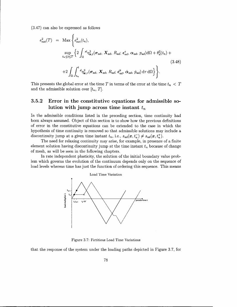
(3.47) can also be expressed as follows

e l J T ) = tv

tn < t< T ' Jn(3.48)

Jn Jtn

This presents the global error at the time T in terms of the error at the time tn < T and the admissible solution over [tn, T}.

3.5 .2 Error in th e con stitu tive equations for adm issib le so­lu tion w ith jum p across tim e instan t tn

In the admissible conditions listed in the preceding section, time continuity had been always assumed. Object of this section is to show how the previous definitions of error in the constitutive equations can be extended to the case in which the hypothesis of time continuity is removed so that admissible solutions may include a discontinuity jump at a given time instant tn, i.e., sad(x, t~) ^ sad(x^t^).

The need for relaxing continuity may arise, for example, in presence of a finite element solution having discontinuity jump at the time instant tn because of change of mesh, as will be seen in the following chapters.

In rate independent plasticity, the solution of the initial boundary value prob­lem which governs the evolution of the continuum depends only on the sequence of load levels whereas time has just the function of ordering this sequence. This means

Load Time Variation

pseudo-tim e t

F igu re 3.7: Fictitious Load Time Variations

that the response of the system under the loading paths depicted in Figure 3.7, for

78

instance, is the same with respect to any value of the fictitious time step A t during which the load level is kept constant. In agreement with this behaviour, it can be assumed that the value of the admissible solution at £+ is also the value at tn + A t and is independent on At. In this way, a fictitious time continuous process over the time interval [tn, tn + At] along which the discontinuity is assumed to be taking place can be defined, and one can analyse the error in the evolution law as the time step A t shrinks to zero.

An example of this process is illustrated in Figure 3.8 which refers to the time

Discontinuous epd(r) Variation

ESd(t„")

Fictitious Continuous £ a d ,A t ( T ) Variation

8«d(tn-l)

. e£d(t);V < ^ 'ir(T) / ......gdfei).

eJd(U)i

(n to+At' tn+At"

Plastic Strain Rate epad A4(t) Variation

[eSd(U)-eTd(t„-)]_L

eJd(u)-£Ed(Ci) t„ - t„_,

[efd(tn) - Efd(tn) ] _L_ At'

E?d(tn.|) ~ £»d(tn) tn.l' tn

{" tn4At' tn+At"

F igu re 3.8: Definition of Fictitious S tate Variables Variation

variation of an admissible plastic strain with discontinuity jump across the time instant tn. Figure 3.8 also hints to the procedure used for the above extension which shows the formation of the 5-Dirac at tn for the plastic strain rate because of the discontinuity jump in eL(t) at tn.

Under constant load level equal to b (x , tn), we consider a family of fictitious time continuous admissible solutions over [tn, tn + At] and parameterized by A t

79

having as limit the given admissible solution, th a t is, we consider

^ad,At{,x i 7")> -^ad,At(«Ej "7”)5 Rad, At(x i <7") >

ead,At(*,T), ead)A4(*,T), a ad)At(*, r ) , Pad,Ai(*>T),

such that, V® E ft,

lim crad,At(x ,r) = &ad{x , r ); lim X adAt(x,T) = X ad{x,r)\At->0+ At—>0+

lim -Rod, At ( a ,7") = Rad(*,r);At—>0+

A1t1iS+ead’A a:;’ ^ = Cad ’ T^; At^+0+^“d’ ^ ^ = €“d^ ’ T^;

^ l im a a d ,A t ( * , t ) = OLad(x, r ) ; J i m + p ad, At (® , r ) = p ad ( ^ , r).

where (•)ad (* ,r) denote the functions with the time discontinuity jump.With regard to each member of this family, the error in the evolution law can

now be computed. Thus, if V x E ft the following limit exists and is finite,

j-tn + A t -

Cd ( X ) ^ n ) = aI^^O-i- I (^ "actA t( * £ , t ) , -X ad , A t (a? , ’7")> ^ a d , A t { X i 7~)) d -J tn

+ <P(<?d>At(a;>'r )> - « a d , A t ( ^ , r ) , -Pad ,A t(x , r ) ) +

- o ’ad .A t^.r): ead,At(x >r ) +

+ ^ad ,A t(^ ,r): a ad, At (a?, r ) + R ad,At ix i T )Pad,At(x i '7") | d r (3.49)

it seems natural to assume the limit to be an error in the constitutive equations at the point x in presence of discontinuity.

R em ark 3.10. The jump in the state variables modifies only the error component that is associated with the evolution law, since these are the equations that involve the rate of the internal variables.

Furthermore, the additional term, A^ ( x , t n), is always non negative as a result of limit of non negative functions due to the Legendre-Fenchel inequality. However, for the material models taken into account, the non negativity of the term A(d(x, tn) will be checked directly. Since A<d{x , tn) > 0, the jump in the admissible solution will always produce an increase of the error component associated with the dissipa­tion. □

80

3.5.2.1 A ugm ented D issipation Error

The dissipation error at the time T of the admissible solution with jump across the time tn E ]0, T[ is given by

Ae2dis(T) = 2 f f drilit(crad, X ad, Rad; epad, 6tad, pad) d t d n + 2 [ A(d(x, tn)dQ. Jn Jo Jn

In order to compute A(sd{x , tv) , the admissible solution is required to satisfy the state equations, which here we present in the following form

<7adAt(X >T) = C[£ad,A*(ah T) ~ (*, t)];(3.50)

X ad,At{x\r) = AotadAt( x ,T ); R adAt{x , T) = g(PadAtix , T))

where A and g(p) are the same as for the plasticity model P2.In the following, we provide the expression for A^d{x, tn) f°r the rate indepen­

dent plasticity models introduced in section 3.2.4.5 by assuming linear hardening. This condition is here invoked in order to guarantee that by assuming a time lin­ear interpolation of the kinematic admissible variables, the corresponding conjugate forces, given by (3.50), will also appear as time linear interpolation of the values at the ends of the time step. This results in the static admissibility of the conjugate forces because of the admissibility of the interpolant values and the convexity of the elastic domain.

Also, for each model, it will be shown that A(d( x )tn) is non negative and that by setting A(,d( x , t n) equal to zero, we infer the time continuity at tn of the admissible solution. This, finally, means that A(d( x , t n) characterizes effectively the discontinuity jump across tn.

Plasticity M odel PI: Prandtl Reuss M odel

Continuous Adm issible F ictitious Solutions.We assume, fl, continuous admissible fictitious solutions defined as follows

□ Kinematic Admissible Solution:£adAt(x iT)'> eadAt(x )r )) PadAt{x i r ) are obtained as linear interpolation over [tn, tn -\- At] of the values at tn and tn + At.

□ Static Admissible Solution:<TadAt(x >T) = C[ead ,A t(^ ,r)-£ ^ )At(cc,r)] and R adAtix , r ) = ^PadAt(x ^r ) are obtained by imposing the state laws. Because of the linearity of these laws, &adAt{x , T) and RadAt{x >r ) are glven by linear interpolation over [tn, tn + At] of the values at tn and tn + At.

□ cradAt(x ,T ) is in equilibrium with b (x , tn) because of the convexity of the equilibrium condition.

81

□ (crad^tiXjT), RadAt{x iT)) £ ® Vr G [£n,£n +A£] because of the convexity of the elastic domain.

Q €ad,At(x iT) is kinematically admissible because of the convexity of the com­patibility conditions.

F inite Value Error RequirementsWe also impose that V x G O the admissible solutions satisfy the following conditions

{(Tad{ x , t - ) , R ad(x , t - ) ) G E

((Tad(x,t+), R ad(x, t+)) G E

=> {&ad(x , t ), R a d i x , r)) G E, Vr G [tn , t n + At], (3.51)

Pad(x ,t+) - Pad(x,t~) > \\epad(x,t+) - e pad(x ,t-)\\,

T r K d & i t n ) - t Pad(X > t n ) ) = 0-

Condition (3.51) occurs because of the linearity of the state laws and convexity of the elastic domain.

D issipation E rror across the tim e discontinuityConsider the expression for the dissipation error for this model given by equation (3.45), we have,

Vx g n

rtn+At (A C ( x , t n ) = AJim / { R o \ \ e Pa d A t ( x ’ T )W +

J tn

~ crad , At (X i T ) ■ £ Pad , At (X ’ T ) + R ad, At ( X >T )P ad ,At (X i T ) } d T =

= flollePad(X ’tn) ~ £Pad(X ’tn)\\ + (3-52)

_ * * ( » , £ ) + * « . ( * , £ ) : (^ (Xj t i ) _ t_ )} +

+ W ) ± ^ M ( h ( l i (+) _ Pad{x> t -))

with the State Equations being satisfied at t~ and £+.

Theorem 3.3.Given the admissible solutions sad(t~) and sad{t^), which satisfy the state

equations at t~ and £+ respectively, and the finite value error requirements, it follows that

ACd(x >tn) > 0

82

P roof. To keep the notation simple, let

c + = crad( x , £+), cr~ = crad( x , £“ );

A c t = cr+ — <j ~\

R + = Radix,t^), R - = Radix, t~)\

A R = R + - R ~ -

Ae = eadix, £+) - ead(x, £~);

AeP = - C O M n );

A p = Pad(iE, £ + ) - Padix, t~).

From the conditions giving a finite value to the error, it follows

Ap > ||Aep|| and R > 0.

Thus we get

i?o|| Aep|| - tr+ : Aep + R +Ap > tf0||Aep|| - er+ : Aep + R+Aep.

Since Tr [A ep] = 0 , we can also write,

cr+ : Aep = cr^ : Aep < ||cr^|| ||Aep||.

Hence,

Ro\\Aep|| - a + : Aep + R +A ep >

> f l„ | |A £l - | | 0-+||||Ae'1|| + R+Ae'- =

= (flo + fl+ - | |o -+ | |) | |A ep|| > 0 ,

that is,i?o|| Aep|| - cr+: Aep + R +Ap > 0. (3.53)

Likewise, it can be proven that

Ro\\Aep|| - (t ~ : Aep + R~Ap > 0. (3.54)

Thus, summing up term by term and for the linearity of the double contractionoperator, it follows

A/-2Q ( x , t n) = 0

T h eo rem 3.4.Given the admissible solutions sad(t~) and sa(*(£+), satisfying the state equa­

tions at t~ and £+ respectively, and the finite value error requirements, the following expressions are valid

' <Tad(x,t+) = (Tad{x, t~)

Rad{X )t^) = R ad(x , tn )

€ad(xt t+) = €ad{x , t - )

ePad(X ^ i ) = €Pad(X ^ n )

k Pad(x,t+) =Pad(x, t-)

P roof. Because of (3.55), by accounting for (3.53) and (3.54), it follows

Ro\\Aep\\ - (T+ : A e p + R + A p = 0

i?o ||A ep|| — & '■ A e p + R~ A p — 0

Thus,

If ACl ( x , t n) = 0

A c t : Aep = A R A p

From equilibrium at t~ and t+ it follows

/ cr~: VrjdQ = / b(x, tn)rjdQ + / t ( x , t n)r)dQ V 7 7 G Vo */ n •/ n J d£it

/ cr+ : V^dQ = / b(x, tn)7jdfi + / t ( x , t n)rjdQ V 7 7 G Vo1/ w n dQt

Hence, since Ae G Vo, subtracting term by term, we get

f A c t: Aedfi = 0 f Acr: (Aee + AepjdQ = 0 Jn Jn

I Acr : A e edfi + f Acr : A e pdQ = 0 Jn Jn

In the dissipation error the state laws are satisfied, i.e.

A ct = C A ee

A R = HAp.

Acr: A ee = C A ee : A ee > 0

A ct : A ep = A R A p = HAp 2 > 0.

Hence, it follows

(3.56)

(3.57)

(3.58)

84

By accounting for (3.56), from (3.57) the following results are obtained

A ct: Aee = 0 A(j = 0 ^ Aee = 0

Acr: Aep = A R A p = 0 => HAp2 = 0 => Ap = 0 ^ Aep = 0

where implication (a) follows from the condition imposed on the admissible solution to deliver a finite error, given by (3.51). □P lasticity M odel P2: Standard variant M arquis-Chaboche m odel

C on t inuous Adm iss ib le Fict i t ious Solut ions .We assume, V x G ft, continuous admissible fictitious solutions defined as follows

□ Kinematic Admissible Solution:£ad,At(x i r )i eldAt(x ’r )’ a adAt(x iT)i Pad,At{x iT) are obtained as linear inter­polation over [tn, tn + At] of the values at tn and tn + At.

□ Static Admissible Solution:o'ad,At(x , T) = C[ead)At(*,T) - epadAt(x,r) \ , X adAt(x , r ) = Aa adAt{x,T) and RadAt(x , T) = Hpad,Ai(®,r).

□ &adAt{x ->T) is equilibrium with b (x , tn) because of the convexity of the equilibrium condition.

Q (<7adAt(x , T)> X adAi{x, r) , R adAti.x i T)) £ E £ [t„, tn + At] because of the convexity of the elastic domain.

□ £adAt{x i r ) *s kinematically admissible because of the convexity of the com­patibility conditions.

Finite Value E rror Requ irem en tsWe also impose that V x G the admissible solutions satisfy the following conditions

(<Tad(x, t"), X ad(x, t~ ) ,Rad( x , t “ )) G E

((Tad( x , T ) , X ad(x ,T ) ,R ad{x,T )) G E

(aad( x , t+ ) ,X ad(x , t+ ) ,Rad(x,t+)) G E(3.59)

Vr G [tn, tn + At].

Padix ,t+) - Pad(x,t~) > IIepad(x,t+) - epad( x , t - ) II,

T ^ K d ^ ^ n ) - ePad(X^n)} = 0 ,

ead(^^n) - cSd(*^n) = 0 =* OLad(x,t+) - a ad(x, t~) = 0. (3.60)

Condition (3.59) occurs because of the linearity of the state laws and convexity of the elastic domain, whereas condition (3.60) derives from the definition (3.28)2 of

85

(p(ep , - a , - p ) .

D iss ipa t ion E rror across the t im e d iscon t inu i tyFor this model we have to distinguish the following two cases in relation to the defi­nition (3.28)2 of the Fenchel-Legendre conjugate of the dissipation pseudo-potential

v x e n

Q IfeS d (* > O -ead0Mn) = 0 then it can also be written OLpad(x, t+)-ocpad{x, t~) = 0 because of (3.60). By accounting for (3.28), the dissipation error takes the following expression

/•tn + AtA ( d ( X > Q = Ajim+ / R a d ,A t(X > T ) P a d A t (X > r )d r =

J tn

= R^ X ’t^ + R<‘<‘(X’tn ) (pad(Xt f+) _ pad(Xi t ~% (3 .61)

with the State Equations being satisfied at t~ and

□ If e^d(x , t^ ) — epd{x, t~) 7 0, and recalling equation (3.28)i, the dissipation error takes the following expression

t'tn+AtA^2,„ / , u ' ~ T)|| +

, C \\epadAt{ x , T ) - a adAt(x,T) \ \2 I \ -p ( \ >2a \ K dAt (x, r ) \ \ <Ta d A x , T). eadAt( x , r ) +

+ X adAt(x,T): OiadAt ( x , T ) + R adAt(X , T)PadA t ( x , T ) } d T =

= Ro\Kd(X ^ i ) ~ ePad(X ^n)\\ +

C W K c i i x , ^ ) - e Pad{ x , t ~) ) - { a ad( x , t + ) - a ad{ x , t - ) ) \ \ 2 2a \\epad( x , t +) - epad(x, t - ) \ \

_ a ad( x A ) + ^ ( x , t ~ ) : (^ (Xj t i ) _ eL(Xi t ; ) ) +

+ X <„ ( x , C ) + X aJ( x , ^ ) : (Qo<j(;Ei(+) _ a a t j ( X i 0 ) +

+ M ^ l ± A i t i S l {pad{^ t+) _ ^ (-)), (3.62)

with the State Equations being satisfied at t~ and

86

T heorem 3.5.Given the admissible solutions sad(t~) and sac/(£+), satisfying the state equa­

tions at t~ and t+ respectively, and the finite value error requirements, it follows that

A(dix i tn) > 0P roof. If Aep = 0 , A a p = 0 ,

A j-O r \ "h R A _Q ( x , t n) = ----- Ap > 0

because of the finite value error requirements.

If Aep ^ 0 ,

O = fioll Ae-ll + ± 11 A | ^ a "2 - +

2 X ~ : A a + —— — Ap. (3.63)

Let us consider the term

«o||Ae'’|| + ^ l |A e ' A 6 ^ Q:|12 - < t : Ae” + X : A a + fiAp, (3.64)

where <r, X , R can all refer either to the time instant t+ or t~. In the following, we will show that (3.64) is non negative, which then determines the non negativity of (3.63).Since,

it follows

Also,

Ap > ||Aep||,

R A p > R\\Aep\\.

a: A ep = a D: Aep = {aD - X + X ) : Aep =

= (aD - X ) : Aep + X : Aep < ||<rD - X\\ ||Aep|| + X : Aep

Hence,-o -: Aep > - \ \ a D - X \ \ \ \ A e p\ \ - X : Aep.

By accounting for the above inequalities, it results

c ||Aep — ArvII f l° ||AePU + Ya ||AeP|| - g : Ae" + X : A a + R A p >

c ||Aep — Arv Ip > Ya ]\AeP\\ + {R° + jR)l|AeP|1 " ll<TD " X |I I |A € P |1 +

- X : (Aep — A a).

87

From the yield condition, it follows

hence,

Also, it follows

(i?0 + R) - \\<rD - X || > - | | X | | 2,Ic

[(Ro + R) - \\<td - X ||] ||A £p|| > - | | X | | 2 ||A£»||

- X : (A ep — A a ) > —||X | | | |Aep — A a | |

so that finally, we have

c IIAep — Arvll^ fio||A6p|| + - l L _ _ .j?ll _ (T: A ep + X : A a + R A p >

+ - H^IIHA^ - Ao.ll ^>

D (365)

T heorem 3.6.Given the admissible solutions sad(t~) and sad(t+), satisfying the state equa­

tions at t~ and t+ respectively, and the finite value error requirements, it follows that

X ad(x, = X ad { x , tn )

ead{x, t+) = ead(x, t~)

^adi.X ^ n ) = cJdOMn)

Oiad( x , t + ) = OLad{x,t~)

Pad{x,t+) = p ad(x, t~)

P roof. We again have to distinguish the two cases in relation to the expression of the dissipation error as given by equation (3.61) and (3.62). We first consider the case of Aep ^ 0 and then Aep = 0 , A a = 0 .

A/-2Cd(X > Ti) — 0

If Aep ^ 0, given the expression (3.62), and accounting for (3.65), it follows

If ACd(x ’ In) = 0 =*■ '

cr+: Ac" = fl0||A«p|| +c ||Aep — A a |

2 a ||Acp||+ R +Ap + X +: Act

■ +

- a d n ii a dii c ||Aep - A a l l «r : A,* = /lo llA el + ||AeP|| " +

+R~ Ap + X ~ : A a

thus,A ct : Aep = A R A p + A X : A a (3.66)

Prom equilibrium at t~ and £+ it follows (see equation (3.57))

/ A ct : AedQ = 0 ^ / Atr: A eedQ + f Acr : AepdQ = 0 (3.67)Jn Jn Jn

In the dissipation error the state laws are satisfied, i.e.

Act CAee

A R = HA p

A X = AA a

hence, it follows

Acr : A ee = CAee : A e e > 0 (3.68)

A ct : Aep = A R A p + A X : A a = HAp2 + A A a : A a > 0

for A is a second order positive definite tensor.By accounting for (3.68), from (3.67) it results

Acr: Aee = 0 => Acr = 0 => Aee = 0

A ct : A ep = A R A p + A X : A a — 0 =>■

HAp2 = 0 => Ap = 0 =£ Aep = 0

A A a : A a = 0 =$■ A a = 0

where implication (a) follows from the condition imposed on the admissible solution to deliver a finite error.

If A ep = 0 , A a = 0 , the dissipation error is given by

H2

A > 2 / ' . \ ^ P R + a H r 4-2 - 2 \Q ( x , t„) = ----- ------A p = - ( p + - p )

89

where we have taken into account the meeting of the state equations at tn and £+. Thus, it follows

ACd(x > tn) = 0 ^ p+2 = p~2 p+ =p~, for p > 0

which deliversAp = 0 =>■ A R = 0

From equations (3.67) and (3.68) we derive also

Aee = 0 => A c t = 0 .

□

3.5.2.2 A ugm ented Extended D issipation Error

The extended dissipation error at the time T of the admissible solution with jump across the time tn G ]0,T[ is given by

A e l x t ( T ) = sup< 2 slr}ltt{<7ad, X ad, R ad] eead, ocad, pad)dHt<r Jn

+

(3.69)

+ 2 [ [ dri i A a «d, X ad, Rad; epad, d ac/, Pad) d r dQ + 2 [ A(d(x, tn)dQ, Jn Jo Jn

where for A(d( x , t n) we consider the same expressions as given in Section 3.5.2.1 . For the applications, it is convenient to rewrite equation (3.69) as follows,

eLt(*n)

A„2 Ieext(T) = m a x ^ sup [ 2 f ^ a n + 2 f [ dn lI t<tn Jn_______ , v Jn Jo

d r d ft

suptt<t<ri

2 f Slll l , t d ^ + e d ( t n ) + 2 [ A £ { x , t n ) d Q + 2 j f dr ] l T d r d n 1 Jn Jn Jn Jtt

(3.70)

A02Atn)

which highlights the different contributions to the error from the parts of the ad­missible solution which are continuous in time.The next result guarantees that definition (3.69) can be assumed as measure of the error in the following sense

90

Theorem 3.7.Given the admissible solutions sad(t~) and sad(£+), meeting the finite value

error requirements and not necessarily the state equations at t~ and £+, respectively, it follows that

A4 t ( r ) > o

A4 t(T) = 0 S a d ( x , t ) = sex(x, t) V a:G ft, V t < T .

P roof. The extended dissipation error Ae\xt(T ) is defined as the supremum of a function which is sum of non negative terms, thus

A „2<xt{T) = 0

e2sl(t) = 0 V t < T <#

ve 2d { T ) = 0 V£ < T

= 0V x G Q, V t < T.

AC = oVrr e SI,

= oVrr G f2, V£ < T.

(a)

( b )

(c)(3 .7i)

Condition (3.71a) means that the admissible solution sad{x, t) satisfies the state laws, V x G ft, V £ < T. This condition along with (3.71b) allows one to conclude also that the jump in all the variables is zero as a result of the argument given in Section 3.5.2.1 for the rate independent plasticity models taken into account. Finally, condition (3.71c) allows to conclude that the time continuous admissible solution satisfies also the evolution law. □

Even for the extended dissipation error a characterization of only the discontinu­ity can be given. Hereafter, the condition is proved only for the Prandtl Reuss model with linear hardening. The argument applies likewise to the standard vari­ant Marquis-Chaboche model with linear hardening. For both the models with more general hardening laws, we believe, however, that similar conclusions can be obtained.

The condition characterizing the discontinuity is next given in a more general format which applies to admissible solutions with jump across time instant t n in the case of rate-independent plasticity.

Denote by

and

{&ad{x, tn), Rad{x , tn) , €ad{x, £n) , €a( (3?,£n), Pad^X, tn))

s ad ( x , tn + At) = ((Tad(x, tn + At), R ad ( x , tn + At)]

€ad(.X, tn -\- At), £ad(x, tn T At), Padix, tn T At))

91

any admissible solution at tn and tn + Ai, respectively, corresponding to the same load level and with sad(t) the admissible solution obtained as time linear interpola­tion over [tn, tn + A i ] of sad{tn) and sad{tn + At). The following theorem, then, can be stated

T heo rem 3.8.Given the admissible solutions sad(tn) and sad{tn + At), corresponding to the

same load level, meeting the finite value error requirements and not necessarily the state equations at tn and tn + At, respectively, it follows Vx G

" Sly, 2 _ Sly, 2 _ S l j lIX, tn lx,tn+ A t 'lx,t

IF < V i G [ in , i n + A i ] .

k ACl,d(X ^n) = 0

tn ) = tn T At)

Radip t tn) = R ad{p i tn T At)

tadipb) tn) = €ad(^, tn + At)

t n ) = ^ a d ( X i + A i )

Padij^i tn) = Padi&i tn T At)

P roof. For the Prandtl-Reuss model with linear hardening, the hypothesis of the theorem concerning the error in the state law writes as

/■Jn(<Tad(t) - Ceead(t)) ■ C (<Tad{t) - C e^ (i))dx +

4 I (Rad(t) - Wpad(t))2dx = const V i G [tn, tn + A i ] .H Jn

Thus, differentiation with respect to time delivers

[ (cTad{t) ~ c eead(t)): C~1(&ad(t) - Ceead(t))dx +Jn

+U / iR ad{t) ~ HPad{t)){Rad{t) - Hpad{t))dx = 0 V i G [ in , i n + A i ]H J Q

which , because of the definition of sad(t), can be written as

(<7ad(t) - c 6 ead(t)): C_1(A(Tad - QAeead)dx +fJn(3.72)

+ U f (R ad{t) - Hpad(t))(ARad - HApad)dx = 0 V i G [ in , i n + A i ]H Jn

where the same notation as in the proof of Theorem 3.3 has been employed provided that t~ is meant as tn and i+ as tn + At.

92

After computing equation (3.72) for t = tn and t = tn + A t and subtracting side to side one obtains

[ (A (Tad ~ C A e ^ ): C- 1(Acrad - C A e ^ d * +Jn

[ (AR ad - HApad) (ARad - HApad)dx = 0 , bl Jn

that is,

[ (Acrad ~ CAeead): C_1(Acrad - CAeead)dx = 0 Jn

pj / (AR ad - HApad)2dx = 0,H Jn

so that the following relations hold

A (Tad - CA€ead = 0

A Rad - HApad = 0,

and the same arguments as in the proof of Theorem 3.3 can now be adopted. □

3 .5 .3 D efin ition o f error in so lu tionLet

S e x ( * £ > 0 = R e x i& i ^)> ^ex(*^5 *^ex(X ) Pexip^i

denote the exact solution of the initial boundary value problem defined in section3.2, that is, sex( x , t ) is the time continuos function that meets all the equations given in Box 3.1.Let

Sa d ( X i t ) = ( u a d ( x , t ) , ^ { x , t ) , a ad( x , t ) , p ad( x , t ) ' ) , (3‘73)

be a kinematically admissible solution with u meeting the compatibility conditions, and e^d(x,t),Oiad(x , t ) ,pad(x,t) meeting the initial conditions. The kinematically admissible solution may also present discontinuity jump across time instants tn. We assume the error in the constitutive equations produced by

Sex,ad = X e x , R e x i ^ a d i ^ a d i ^ a d i ' P a d ' j i

as global measure of the exact error in solution associated with sktd .This is defined as

elx(T ) = s u p ^ x W . ( 3 -7 4 )t< T

93

where

„o , v I «; o «_______ ___^ex( 0 2 I X ex, R exi £adi ^adj Pad)dfi

dO

+ 2 / / S a .r^ e z , X e;r, Rex> ^ad’ ^ad? Pad) dQ. do do

The following heuristic argument show that this definition of error is meaningful. First, note that

( (aex, X ex, Rex) e E V x G fi, Vt < T (a) e2ex{T) FINITE => (3.75)

I «ad, Pad) GC V x G fi, \ / t < T (b)

where E x C is the effective domain of the function dp^(<r, X , /?; ep, a , p)- Forthe plasticity models under consideration, if the admissible solution is discontinuous across the time instant tn, conditions (3.75b) imply that

Apad > | |A < J | . (3.76)

Now, we can give the following result:T heo rem 3.9.

Given a kinematic admissible solution s^ n = ( u ad,e^d,cxad,padj , it followsthat

e2ex(T) = 0 IF and ONLY IF

P roof. Denote with

Sex,ad is time continuous

Sex,ad{x, t ) = Sex( x , t ) Vx G Q, V t < T

o- = C[ead - epd],X A.OLad)

R = g ( P a d )

the forces conjugate to the admissible kinematic variables (ead, e^d,pad, otad).Since e2ex(T) is defined as the supremum of a function which is sum of :terms, it follows

eL(T) = 0 ^ •r s,vi,t = o'i . „

v x g n , V* < T, (a)

I dvl,t = o Vcc G fl, V£ < r . (b)

Condition (a) means that

cf(:r, t) = & ex (® > 0 Vx g n , V£ < T,

X ( x , t ) = X ex(x, £) Vcc G \ / t < T,

R(x, t) = R ex (*®» 0

94

Va: G Q, Vt < T.

Because of the time continuity of (crex( x , t), X ex( x , t), R ex( x , t)) and of the continu­ity of the functional relations that define the state equations, the time continuity of (ead> Pad, otad) also follows. In turn, the time continuity of pad, along with the condi­tion (3.76) implies also the continuity of evad, hence the continuity of ead = e ^ + e ^ , as well. Then, it follows that

Uadi ^ adi ^ adi Pad'j $ex,ad

is time continuous, statically admissible, meets the state laws and the evolution laws. Thus it coincides with the exact solution, sex. □

3.5.3.1 Extension of the Prager-Synge theorem to the D issipation Error

In the case of the dissipation error, for a time continuous admissible solution s ad , Ladeveze (1999) shows that the following equation holds for a normal formulation of the model

I I adi X adi Radi ^ adi Pad) d.T dSl —Jn Jo

— q I (&ex G"ad) ■ C (&ex O’ad)d01 Jn

i f ( X „ - X ad) : A - ^ X ^ - X J )* Jn

« [ {Rex ~ R a d ) ^ 1 ( R ex - Rad)1 Jn 1

f [ dr)lyT{sadi sex) dr dtt Jn Jo

+

+ -

t

dCl

dn (3.77)

where

with

d„2Vx , t ( Sadi S e x ) Vx, t(^ex,ad) Vx , t i Sad,ex)

Sex,ad ex> -^en Rexi u adi a ad,Padj >

$ad,e x — ^&ad, X ad, Rad', U e x i £ Ve x i C X - e x i P e x ' j ,

which can be easily obtained by elaborating on the expression of TQt{sad) andaccounting of the properties of the exact solution sex.

Equation (3.77) can be considered as an extension of the Prager-Synge theorem to the Dissipation Error and, likewise for the linear elasticity, allows one to show easily that the dissipation error is an upper bound for the error in the solution asdefined by equation (3.74). Indeed, we have the following result:Theorem 3.10.

Given an admissible solution, sad, with respect to the computation of the dissipation error, it follows

4i, (T) > e l ( T ) (3.78)

95

P ro o f. Let

= / {^ex ~ ^ad) ■ C 1 {<Tex - a ad)dQJn

+ f {.X ex- X ad):Jn

+ [ {Rex ~ Rad) H 1 {Rex ~ Rad)Jn L

+2 [ [ dr)l,T{sex,ad) drJf2 JO

+t

+

and

= 2 [ f dr)ltT{sad) dr dQ.Jn Jo

Since dr}lT(sez>ad) > 0 and drfcr (sad,ex) > 0, it follows from equation (3.77),

fi(t) > e l { t ) vt < t .

Thus, it issup62d{t) > s\ip92ex{t) = e2ex{T)t< T t< T

wheresup 03(f) = fl3(T) = e L (T),t< T

since 6d(t) is an increasing function of time. □

3.6 Concluding RemarksThis Chapter represents the theoretical core of the thesis. Here, the theory of the error in the constitutive equations for material models with internal variables and associative flow rule has been presented following the works of Ladeveze (1989) and Ladeveze et al. (1999).

The fundamental notion of admissible solution has been given. The error in the constitutive equations developed by Ladeveze et al. (1999) has been extended to admissible solutions with discontinuity jump at the time instant tn in the case of rate-independent plasticity models. Theorem 3.8 represents the main proposition of the Chapter. The theorem provides a characterization of the discontinuity jump in the admissible solution as a function of the augmented term d(x ^n) and of the behaviour of the error component associated with the residual in the state law.

As a result, the augmented extended dissipation error can be employed as a basis of methodology for the assessment of the global accuracy in time of finite element solutions on evolving meshes.

96

With this regard, in the next Chapter we first recall the governing finite element equations and subsequently, we continue discussing the several sources of discretiza­tion errors which are introduced, in particular those arising from the change of finite element mesh from one time increment to the other.

97

Part II

Application to the Finite Element Solution of the IB V P in

Elasto-Plasticity

98

Chapter 4

The Finite Element Solution of the IBV P in E lasto-Plasticity

4.1 IntroductionIn this chapter we report on the displacement finite element method for the solu­tion of the initial boundary value problem of an elastoplastic model with internal variables. After reformulating the general problem in a way which presents the displacement field u = u (x , t ) G V as the sole principal unknown, we continue by discussing the corresponding discrete schemes so that the nature of the ensuing discretization errors can be understood.

With this regard and the aim to set a general framework for handling evolving finite element meshes, we need to invert the usual sequence of first spatial and then temporal discretization by considering first the semidiscrete scheme in time, which is here obtained by a backward Euler integration in time. The initial boundary value problem, continuous in time and space, is transformed into the recursive solution of nonlinear problems, continuous with respect to the space, which are referred to as incremental boundary value problems, henceforth abbreviated as InBVP. In these problems, the state of the system at the time instant tn is a data of the problem, whereas the principal unknown is the displacement field at the time instant tn+

The fully discrete scheme of the initial boundary value problem is therefore ob­tained by a finite element discretization of these incremental boundary value prob­lems. This is obtained by replacing the general infinite dimensional affine spaces where the principal unknown and test functions belong to, with finite dimensional affine spaces. Here, we observe that change of data and/or of finite element mesh from one time interval to the other can be both related to a discontinuity jump of the approximate solution across the time instant tn. As a result of the observations expressed in Section 3.4, in the developments of reliable a posteriori error estima­tors, one needs, therefore, to account also for the jump. With such a posteriori error estimator at hand, indication on how to change the finite element space and define the corresponding data can be given and the assessment of the several transfer operations proposed in literature can be framed in the context of the ensuing error.

99

We, therefore, will give a brief review of some of the current techniques to trans­fer data from one mesh to the other, and recall the numerical techniques adopted for the solution of the nonlinear algebraic system of equations before concluding the chapter.

4.2 The displacement formulation of the IBVPIn section 3.2 the properties and equations that define the behaviour of a standard generalised material model have been given, which for the reader’s convenience have been summarized in Box 3.1. There, the constitutive equations were presented in the alternative scalar equivalent formulations for the purpose of the theory of the error in the constitutive equations. The latter are now given in a more general format, not necessarily restricted to the class of standard models, which is used as basis of the numerical discretization. The general formulation of the problem, therefore, reads as in Box 4.1 where # and 0 denote two multivalued tensorial functions which assure the thermodynamic admissibility of the model and enjoy the necessary regularity properties to guarantee a solution of the constitutive initial value problem for given total strain. Furthermore, as for the specific choice of the functional spaces, that is, of the functional setting in which the initial boundary value problem is posed, in the following we assume, if not stated otherwise, that the spaces are endowed with those minimum regularity properties that make the operations involved meaningful and guarantee at least the existence of a solution, (Brezis, 1986; Fiorenza, 1988). However, given the generality of the formulation in Box 4.1, in the current literature, there are no results on its well-posedness. These are available only for some special classes of material models and for some formulations of the initial boundary value problem, as it can be found, among others, in the works of Moreau (1974); Duvaut & Lions'(1976); Johnson (1976a, 1978); Suquet (1981); Temam (1985, 1986); Han & Reddy (1999); Alberty & Carstensen (2000) and Fuchs & Seregin (2000).

R em ark 4.1. We would like to point out the two main techniques which have been adopted for the proof of existence of solutions and which differentiate mainly in the first part of the proof. One makes a systematic use of Rothe’s method (Kacur, 1985) in which first approximate solutions are constructed by semidiscretization in time, and then one passes to the limit using compactness arguments. The other technique applies the methods of the constructive theory of partial differential equa­tions in which a family of regularized problems is examined before passing to the limit using likewise compactness arguments (Evans, 1999). For both the techniques it is fundamental that uniform a priori estimates of the approximate solutions are available. □

100

Box 4.1. General formulation of the Initial Boundary Value Problem for amodel with internal variables

Given b ( x , t ) on fl, t ( x , t ) on dVLt and the initial state (here assumed as free)

Find W G [0, r]u = u(«, t) G V

ev = ep(*, t ) e £

a. = a(», t) G A

cr = cr(«, t) G S

A = A(», i) £ d

such that the following equations are satisfied:

(<t(x, t), V77(x)> = (b(x, t), f/(x)> + (t(x, t), r)(x))sti,

V r j e V o , Vt 6 [0 ,T],

and, Vx G Vt G [0, T],

e(x, t ) = V5u(x, £)

C onstitutive Initial Value Problem (C IV P)

e(x, t ) = ee(x, t) + ep(x, £)

A(x,£) = ^ ( a ( x , t ) )

dtep( x , t ) G £(<t(x,£), A(x,£))

<9ta(x ,£ )G 0(er(x, i), A(x, £))

ep(x, £ = 0) = 0

a(x , £ = 0) — 0

101

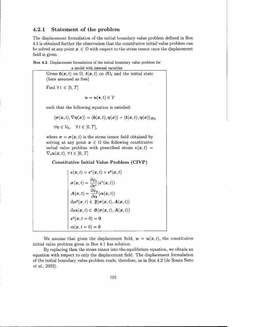
4.2 .1 S ta tem en t o f th e problem

The displacement formulation of the initial boundary value problem defined in Box4.1 is obtained further the observation that the constitutive initial value problem can be solved at any point x e Q, with, respect to the stress tensor once the displacement field is given.

B ox 4.2. Displacement formulation of the initial boundary value problem for a model with internal variables

Given b(x, t) on Q, t(x, t ) on dQ,t and the initial state (here assumed as free)

Find Vt G [0, T]

u .= it(«, t) G V

such that the following equation is satisfied:

( t r (x , t ) ,V rj(x)) = (b(x , t) , i j (x)) + ( t(x, t),rj(x))an,

VrjeVo, V ie [0,71,

where cr = cr(x, t) is the stress tensor field obtained bysolving at any point x G the following constitutiveinitial value problem with prescribed strain e(x, t) =V su ( x , t ) , \ f t e [0, T\

C onstitutive Initial Value Problem (C IV P)

e(cc, t) = ee( x , t) + ep(x, t)

A (x , t ) = ^ ( a ( x , t ) )

dtev(x, t) G $(<T{x,t) ,A(x, t))

dta ( x , t ) e 8 ( ( r ( x , t ) ,A (x , t ) )

ep(x, t = 0) = 0

a ( x , t = 0) = 0

We assume that given the displacement field, u = u(x , t ) , the constitutive initial value problem given in Box 4.1 has solution.

By replacing then the stress tensor into the equilibrium equation, we obtain an equation with respect to only the displacement field. The displacement formulation of the initial boundary value problem reads, therefore, as in Box 4.2 (de Souza Neto et al., 2 0 0 2 ).

102

R em ark 4.2. The solution of the constitutive model with respect to the stress tensor in terms of the displacement field is implied, on a conceptual level and under general smoothness assumptions, by the equivalence of the two type of formulations of a constitutive model, the one in terms of the history of the mechanical variables and the other in terms of the internal variables (Bataille k Kestin, 1979; Ladeveze, 1999). Also, it is worth mentioning that the solution of the constitutive initial value problem (henceforth abbreviated as CIVP) with prescribed strain field e ( x , t ) = V su (x , t ) delivers the field of all the variables which describe the state of the system (Laborde k Nguyen, 1990). □R em ark 4.3. A formal expression of the problem given in Box 4.2 in the case of perfect plasticity with the equation expressed only in terms of the displacement field can be found, for instance, in Rannacher k Suttmeier (1998). This formulation is, in fact, not different from the one given in Box 4.2 since the authors let cr = Il(Vw) where II denotes a very general operator obtained by solving the CIVP with respect to u. □

4.3 The time discrete problemThe displacement formulation of the initial boundary value problem given in Box4.2 is discretized in time by the backward Euler method. This is the time discrete scheme which will be the focus of our considerations in the following because of its stability and accuracy properties for finite time step (Ortiz k Popov, 1985).

Let 0 = t\ < . . . < tn < . . . < tN+i = T be a partition of the time interval of interest [0, T] and set k = max {kn = £n+1 — tn}. A family of fully implicit

l < n < Napproximations of the problem in Box 4.2 is obtained as recursive solution of the non linear spatially continuous variational problems defined in Box 4.4. These are obtained by replacing the rate quantities with backward difference quotients and by sampling all the other functions at £n+i- Thus, the constitutive initial value problem is transformed into the constitutive incremental nonlinear problem (hence­forth, abbreviated as CInNP), and the resulting global problem appears, therefore, in the form of a system of variational equations, which expresses the equilibrium, and unilateral constraints in the presence of the inclusions which define the stress tensor field. This format is much clearer if, for instance, we refer to the model of linear elasticity and associative plasticity with linear hardening (Simo k Hughes, 1998; Rannacher k Suttmeier, 1998; Han k Reddy, 1999), which is given in Box4.3. Here, the CInNP is obtained by backward Euler discretization of the principle of maximum plastic dissipation (3.17).

The effect of replacing the time derivative with backward difference quotients produces an error which is referred to as the time discretization error. The main effect of this error is visualized in Figure 4.1 for a model of perfect plasticity with regard to the error on the direction of the plastic flow under the assumption that the point x experiences plastic loading passing from tn to £n+i. However, also an error in the intensity of the plastic flow must be noted, in general. The magnitude

103

Box 4.3. Fully implicit scheme of the IBVP for the model of linear elasticity andassociative plasticity with linear hardening

For: n = 1 ,2 , . . . , N

G iven: External Loading bn+1(*®) — fr(®, ^ n + l ) , OH ^t n+i(x) = t{9, tn+1), on dQt

State of the system at tn el (x) = e p(»,tn) e £ a n(x) = a(* , tn) G A

Find: Un+l(x) = «(•,£„+1) E V

Such T h a t the following equation is satisfied:

(crn+1(®), Vrj(x)) = (bn+i(x),rf(x)) + (tn+i{x), rj(x))dQt V77 G V0,

with crn+i(x) = <r(x,tn+1) E E n+i(a:), where Xn+i(cc) is obtained by solving at any point x E fl the following variational inequality defined by the prescribed strain e (x , t n+1) = Vsu n+i(cc),

- ^ n + iW ): C 1{r(x) - crn+1(;r))+

+ (H a n(x) - A n+i ( x ) ) : H ~ \ B ( x ) - A n+1(x)) < 0

V ( r , B ) e E

where^ n T i ' M = C(Vsu n+1(x) - epn{x))

of this error depends on the accuracy for finite time step of the time integration scheme. This accuracy is, usually, assessed numerically with the so-called isoerror maps (Krieg Sz Krieg, 1977; Schreyer et al., 1979; Ortiz & Popov, 1985).

In proposing the above time discrete scheme, we are faced with two questions: one refers to the existence and uniqueness of the solution for the single nonlinear variational problem while the second regards the convergence of the family of the approximations with their respective rate. Unfortunately, for the formulation given in Box 4.4, likewise the continuous formulation, there are no general results of well posedness and, a fortiori, of convergence of the approximation. However, some considerations can be done in merit, though of heuristic character, as extension of those holding for formulations for which a complete analysis has been provided by Han & Reddy (1999).

In stating the single one step variational problem relative to [tn, tn+1], the state of the system at the time instant tn defined by ep(x), ctn( x ) is a data of the

104

tn+]

E f (a )= 0

F igure 4.1: Effect of the time discretization error in the direction of the plastic flow, ep(t) «

n+-- with t 6 [£n , tn+i] for a perfect plasticity model with yield surface given by equation

f(<?) = o.

problem whereas the unknown is given by the function u n+\(x). Therefore, we assume that the single nonlinear variational problem has solution, as long as very general regularity properties are met by the data. This can be easily shown, for example, for the time discrete scheme of the dual variational formulation for the model of linear elasticity and associative plasticity with linear hardening, given in Han h Reddy (1999), where (u , ct, A ) are assumed as primary variables and the change of data corresponds to the projection onto a closed convex set at a different point.

Also, we require that e£(:c), a n(x ) are obtained from the pointwise solution of the CInNP relative to the previous time interval [tn- 1, tn] and to the solution u n(x). This condition, which can be expressed as continuity of the piecewise linear interpolant of the discrete solutions { e ^ a ? )} ^ 1, { a n(a;)}^r=j'11, is invoked in order to obtain an a priori estimate for the family of solutions which is independent on k. This is a basic result which is used for a compactness argument to prove finally that as k —> 0, the limit of the interpolants is in fact a solution of the continuous problem. Part of the analysis of the semidiscrete scheme would be also an a priori error estimate of the approximate solutions which would have in general the following format

max. \ \uex( x , t n+1) - u n+i(a;)|| < 0(/c9), q > 0, (4.1)l < n < N

which describes the time discretization error with its dependence on the discretiza­tion parameter k along with its rate of convergence and ||«|| is an appropriate norm.

R em ark 4.4. In relation to the particular constitutive model, the solution of CInNP can result in more or less complex algorithm. The procedures for its solution are generally called constitutive update algorithms. In rate independent plasticity mod­els, in particular, they are also referred to as the stress return algorithms, because the stresses must be returned to the yield surface (Ortiz & Stainier, 1999). For an overview of these procedures, we refer to Simo (1998); Armero & Perez-Foguet

105

Box 4.4. Fully implicit scheme of the problem given in Box 4.2

For: n = 1, 2 , . . . , N

G iven: External Loading

State of the system at tn

bn+1(x) = b(m,tn+i), on n tn+i(x) = * (• ,£ „+ 1)> on

e n ( x ) = e p{»,tn) e £a n(x) = a ( » , t n)G A

Find: u n+l(x) = u (« ,tn+1) G V

Such That the following equation is satisfied:

(an+1{x), Vrj(x)) = (bn+1{x),rj{x)) + (tn+l{x) ,rj(x))dnt V?7 e V0,

where a n+i ( x ) = <r(cc, tn+1) is the stress tensor field obtained by solving, at any point x G Q, the following constitutive nonlinear problem with prescribed strain e ( x , t n+1) = Vsu n+1(cc),

C onstitutive Increm ental Nonlinear Problem (C InN P)

e(x, tn+1) = ee(x, tn+1) + ep(x, tn+1)

. . d'lpe . . . .( T { X , t n + 1) = — ( c ( * , t „ + 1 ) )

. . d'ipp. . .A \ x , t n+1) —

ep(:r,£n+i) - ep(x,£n) N ^

a (®, t n+i) - a ( x , t n) _ \\G ©(<x(£c, ), A \ x , tn-\.\))

rCrJ

(2002) and de Souza Neto e£ al. (2002). □

We conclude this section by observing first that the nonlinear variational prob­lem of Box 4.4 can be given the following compact form of a nonlinear variational

106

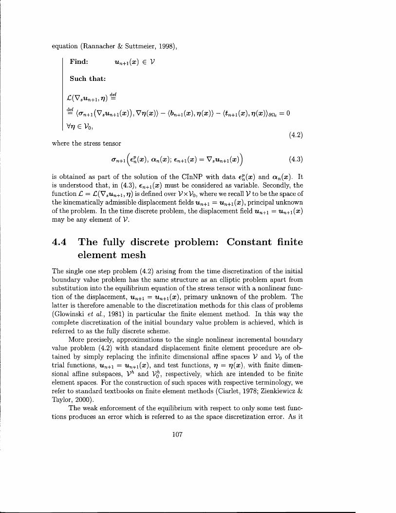
equation (Rannacher & Suttmeier, 1998),

Find: u n+i(x) € V

Such that:

£ { V au n+1 , 77) =f

=f (<rn+i ( V su n+i ( x ) ) , V tj(x )) - (bn+i(x), T}(x)) - (t n+i(x),T](x))dnt = 0

Vry G V0,(4.2)

where the stress tensor

0n+ i( e ^ x ) , olu{x ); en+i(x) = V su n+i(a:)) (4.3)

is obtained as part of the solution of the CInNP with data e^{x) and a n(x). It is understood that, in (4.3), en+i(x) must be considered as variable. Secondly, the function C = £ (V sn n+i, rj) is defined over Vx Vo, where we recall V to be the space of the kinematically admissible displacement fields u n + 1 = u n+i(x) , principal unknown of the problem. In the time discrete problem, the displacement field u n + 1 = u n + 1 (x) may be any element of V.

4.4 The fully discrete problem: Constant finite element mesh

The single one step problem (4.2) arising from the time discretization of the initial boundary value problem has the same structure as an elliptic problem apart from substitution into the equilibrium equation of the stress tensor with a nonlinear func­tion of the displacement, u n + 1 = u n+i(x) , primary unknown of the problem. The latter is therefore amenable to the discretization methods for this class of problems (Glowinski et al, 1981) in particular the finite element method. In this way the complete discretization of the initial boundary value problem is achieved, which is referred to as the fully discrete scheme.

More precisely, approximations to the single nonlinear incremental boundary value problem (4.2) with standard displacement finite element procedure are ob­tained by simply replacing the infinite dimensional affine spaces V and Vo of the trial functions, u n + 1 = u n+i(x), and test functions, 77 = rj(x), with finite dimen­sional affine subspaces, V and Vq , respectively, which are intended to be finite element spaces. For the construction of such spaces with respective terminology, we refer to standard textbooks on finite element methods (Ciarlet, 1978; Zienkiewicz & Taylor, 2000).

The weak enforcement of the equilibrium with respect to only some test func­tions produces an error which is referred to as the space discretization error. As it

107

has been already noted for linear problems in Section 2 .2 , the main effect of this error is the lack of the pointwise equilibrium over the domain fl, along the bound­ary traction dQ,t and the element boundaries. The latter, in turn, means lack of continuity of the stress tensor field therein.

The discrete problem relative to the time interval [tn, tn+1] reads as follows

Given: External Loading bn+i(x) , on Qt n+i(cc), on dQt

State of the system at tn eP(x) G 8 olu{x ) G A

Find: Un+1(*) € V'

Such T h a t(hcrn+1(x), Vr]h(x)) = {bn+1(x),Tjh(x)) + (tn+1(x) ,rjh(x))dni

y v h e v£,(4.4)

where the stress tensor field hcrn+i{x)^ is the function defined by solving at any point x G H the CInNP for any given strain e£+1(a?) = V su^+1(x) and fixed datae n ( X ) > a n ( x ) .

Since a complete theory for the fully discrete approximations to the displace­ment formulation of the initial boundary value problem is still to be developed, the considerations that follow will have, therefore, heuristic character and will assume minimum regularity requirements. In rate independent plasticity with positive hard­ening, this leads, in our case, to the assumption that ep(x, t), cx(x, t ) are continuous in time and in space, whereas ep(x, t), 6l(x, t ) can experience discontinuity in time.

R em ark 4.5. The following observations take their motivation primarily from the analysis of fully discrete approximations to other formulations of plasticity, basically the dual variational formulation of the model of linear elasticity and associative plas­ticity with linear hardening (Johnson, 1976b, 1977; Hlavacek, 1980; Han & Reddy, 1999) and of other evolutive processes, in general, (Kacur, 1985; Evans, 1999) and in particular, parabolic equations (Raviart Sz, Thomas, 1983), and degenerate parabolic equations (Nochetto et a/., 1997; Chen et al , 2000a). Instrumental is also the work by Dorfler k, Wilderotter (2000), though for elliptic problems, on the development of a posteriori error estimates which account for data error. □

Likewise the Galerkin finite element approximation of the primal formulation of an elliptic problem, we can, therefore, assume that the results of well posedness

^ Hereafter, the symbol h(») will refer to secondary variables which are obtained from the solution of the CInNP for the prescribed strain e£+1. They do not have to be confused with the respective finite dimensional discretizations, which are here not considered. Only the interpolation of the prim ary variable, th a t is, the displacement field, has been assumed which is remarked with the superscript h on the right.

108

for the continuous problem (4.2) carry over also to its finite element counterparts represented by problem (4.4); in particular, we emphasize the existence of solution as long as the data ep(x), atn( x ) satisfy general regularity properties.

The result of the approximation which involves only the unknown function u n+i ( x ) is an error whose value depends on the approximation properties of the finite element subspaces. This is usually mirrored by an a priori error estimate of the discretization error which is of the following type

\\un+i(x) — u^+1(x)|| < 0 ( h p)

where h denotes the mesh size of the triangulation 7^ of the domain Q, associated with the finite element space Vh, and u n+i ( x ) is the solution of the continuous problem (4.2). If we combine the above result with (4.1) and use the triangular inequality, finally, we can obtain

max \\uex{x, tn+1) - u^+1{x)\\ < 0 { k q) + 0{hp) (4.5)l<n<JV

which shows the effects of time and space discretization on the full discrete approx­imation along with their respective order of convergence.

In posing problem (4.4), however, the data epl{x)^cxn{x) are unknowns, for being solution at tn of the time discrete scheme. Therefore, a fully discrete approx­imation to the problem (4.2), actually, calls also for an approximation to the data of each nonlinear incremental boundary value problem.

If the finite element space Vh does not change from one time interval to the other, a fully discrete scheme is formulated by assuming the data he^(x)^ hatn(x), which denote the pointwise solution at tn of the CInNP with /le^_1(a?), hatn- i (x ) and prescribed strain €^(x) = Vsit^(x) corresponding to the finite element solution at tn. As a result of this choice, the piecewise linear interpolant of the discrete solutions { ^ ^ ( x ) } ^ 1, {/lo:n(cc)}^j11, is continuous. By exploiting then properties of the equations, one can, therefore, envisage to get a uniform a priori estimate for the family of solutions which proves to be crucial for the error analysis of the fully discrete scheme as it results from the convergence studies carried out in Johnson (1976b, 1977); Hlavacek (1980) and Han & Reddy (1999) which finally deliver an error estimate in the form of relation (4.5).

The above considerations suggest that also other approximations to the data of(4.2) can be imagined, provided that then it is possible to prove the convergence of the resulting fully discrete problems. However, the effects of different approximations to the data from the one proposed above and of change of finite element space from one time step to the other, necessary in the adaptive finite element solution of the given initial boundary value problem, are similar and related somehow to each other. Both can be related, in fact, to the introduction of a discontinuity in the solution as it will be shown in the next Section.

109

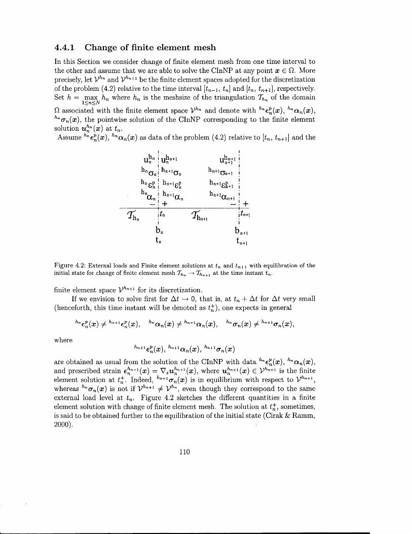
4.4 .1 C hange o f fin ite elem ent m esh

In this Section we consider change of finite element mesh from one time interval to the other and assume that we are able to solve the CInNP at any point x E Cl. More precisely, let Vhn and Vhn+1 be the finite element spaces adopted for the discretization of the problem (4.2) relative to the time interval [£n- i , tn] and [£n, tn+1], respectively. Set h = max hn where hn is the meshsize of the triangulation 7^ of the domain

l<n<NCl associated with the finite element space and denote with hne^(x), hna n{x ), hnern(x), the pointwise solution of the CInNP corresponding to the finite element solution u^n(x) at tn.Assume hnevn(x), hna n( x ) as data of the problem (4.2) relative to [tn, tn+1] and the

u£" U„n+1 i i h n + 1u n+l

hna„ h n + 1 <7n h n + l CTn+1

hnpph na „

h n + l c P

hn+1a n+

hn+1eS+ihn+1a n+i

I tn I

b„t n

Tvh n + l

+-I----\tn+\

n+1

'n+1

F igu re 4.2: External loads and Finite element solutions at tn and t n+1 w ith equilibration of the initial sta te for change of finite element mesh 7/ln —> %,n+1 at the time instant t n .

finite element space V/ln+1 for its discretization.If we envision to solve first for At —> 0, that is, at tn + A t for A t very small

(henceforth, this time instant will be denoted as £+), one expects in general

hne pn {x ) ± hn+' e P ( x ), hna n ( x ) ± hn+lotn( x ), hnarn ( x ) ± hn+1a n { x ),

wherehn+1e l ( x ) , hn+1a n ( x ) , hn+1a n ( x )

are obtained as usual from the solution of the CInNP with data hne^(x), hnatn( x ), and prescribed strain e^n+1( x ) = V su^ n+1 ( x ) , where u!^n+1( x ) G Vhn+1 is the finite element solution at t+. Indeed, hn+1crn( x ) is in equilibrium with respect to Vhn+1, whereas hna n ( x ) is not if Vhn+1 Vhn, even though they correspond to the same external load level at tn. Figure 4.2 sketches the different quantities in a finite element solution with change of finite element mesh. The solution at £+, sometimes, is said to be obtained further to the equilibration of the initial state (Cirak & Ramm, 2000).

110

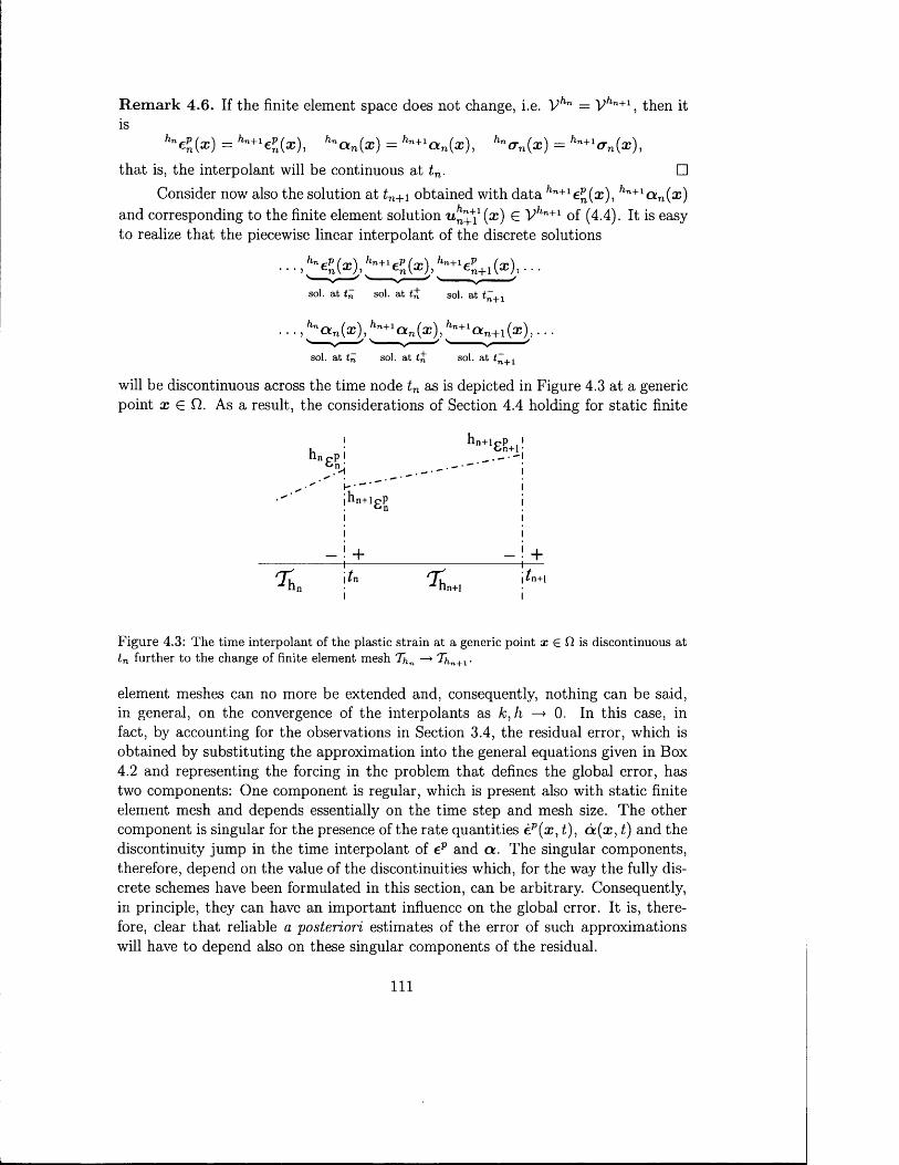
Remark 4.6. If the finite element space does not change, i.e. V hn = V/ln+1, then it is

hnepn{x) = hn+1epn( x ), hna n(x) = hn+1a n{x), hncrn{x) = hn+1crn{x ),

that is, the interpolant will be continuous at tn. □Consider now also the solution at £n+1 obtained with data /ln+1e^(cc), hn+1otn( x )

and corresponding to the finite element solution E y ^ 1 of (4.4). It is easyto realize that the piecewise linear interpolant of the discrete solutions

sol. a t tn sol. a t t£ sol. a t t~+1

.. ■,^ q n(4 ^ 1a n(a ) , illB+1an+1(a!), . . .

sol. a t tn sol. a t sol. a t

will be discontinuous across the time node tn as is depicted in Figure 4.3 at a genericpoint x E fh As a result, the considerations of Section 4.4 holding for static finite

ih n + l£ n + lnn cp i

.•H

• |h n + lp P

11

- ! + +

i^ nI ln1

% n +i^n+1

F igure 4.3: The time interpolant of the plastic strain at a generic point x G is discontinuous at tn further to the change of finite element mesh Thn —» Thn+X-

element meshes can no more be extended and, consequently, nothing can be said, in general, on the convergence of the interpolants as k, h —> 0. In this case, in fact, by accounting for the observations in Section 3.4, the residual error, which is obtained by substituting the approximation into the general equations given in Box 4.2 and representing the forcing in the problem that defines the global error, has two components: One component is regular, which is present also with static finite element mesh and depends essentially on the time step and mesh size. The other component is singular for the presence of the rate quantities ep( x , £), 6t(x, t ) and the discontinuity jump in the time interpolant of ep and a . The singular components, therefore, depend on the value of the discontinuities which, for the way the fully dis­crete schemes have been formulated in this section, can be arbitrary. Consequently, in principle, they can have an important influence on the global error. It is, there­fore, clear that reliable a posteriori estimates of the error of such approximations will have to depend also on these singular components of the residual.

I l l

R em ark 4.7. Convergence studies of fully discrete approximations in presence of changing mesh are completely missing from the current literature, even for those variational formulations of plasticity models which have been investigated in detail in the case of finite element mesh constant in time. Furthermore, it must be noted that the issue of convergence of fully discrete approximations in presence of evolving finite element meshes is shared also by other evolutive processes, in general, as it has been pointed out since by Dupont (1982). This problem, actually, calls for constraints on the type of change of mesh as shown in Nochetto et al. (1997) and Dawson & Kirby (1999) in order to deliver family of discrete schemes that are stable and convergent. Also, it is interesting to note in the a posteriori error estimates of these approximations the presence of terms that are due to change of mesh (Eriksson & Johnson, 1991; Estep et a/., 2000; Chen et a/., 2000a). □

In conclusion, if no change of mesh occurs, k and h are the only parameters that control the accuracy of the approximation, thus, both a priori and a posteriori error estimates will depend somehow on them. On the contrary, if change of mesh occurs, we introduce a discontinuity in the solution which can be arbitrary. The residual will have singular components depending on the jump. Since the error depends on the residual, its estimates, both a priori and a posteriori, will have to account for the discontinuity.

Also, the considerations expressed in this section point out an important issue in presence of change of mesh. This is the development of a posteriori error estimates which by including terms that depend on the jump allow one to assess the effects of change of mesh and data for the solution of (4.4). We will see in Chapter 6 how the error in the constitutive equations will permit to account for the discontinuity in a natural and consistent way.R em ark 4.8. A similar outcome, though starting from a different point of view, can be retrieved from the analysis carried out in Rannacher & Suttmeier (1999), which has been highlighted in section 2.3.2. The authors refer to a dual variational formulation of plasticity and propose a splitting of the error which distinguishes the component due to time discretization, to the space discretization and to the effect, through the stability of the nonlinear incremental boundary value problem, of the error for using different data in posing this problem. □

4.5 Overview on the different definitions of the initial state. Transfer procedures

In the previous section, we have assumed the data hne^(x), hna n( x ) to be known at any point x G f i and equal to the solution at tn relative to the previous time interval [tn- 1, tn]. However, in the actual computation, we do not need in general to know such fields but only their value at discrete points, namely the integration points of each element. In fact, the integrals that appear in the variational formulation (4.4) are seldom computed exactly. Instead, they are approximated through a process of numerical integration, such as, for instance, Gaussian quadrature formula.

112

Let Qgn+1 G Thn+l be a generic element of the triangulation 7^ n+1 and denote with x ^ +1 G Ogn+1 the ith Gauss point of the element Qgn+1 and ngp their number. Problem (4.4), formulated next with generic data e£(cc), a n(x), reads as

G iven: V fign+1 G %in+1 and for i = 1 , . . . , ngp ,

External Loading

State of the system at tn

Find: U n + l ( X ) ^ Vhn+1

Such th a t:ngp

(4.6)where the stress tensor /ln+1o-n+i ( e ^ 1(cCgj"+1) = V ( # e , i +1)) obtained by solving at the CInNP with data e£(cCgi"+1), d n(cCg"+1) and prescribed strain

in Gaussian quadrature scheme for which we refer to Ciarlet (1978); Zienkiewicz & Taylor (2000) and de Souza Neto et al. (2 0 0 2 ). Also, note that for the sake of notation, we have dropped the work of the traction forces in (4.6).

The choice of the quantities in rate form as secondary variables, for which no a priori interpolation assumptions have been made, and the use of backward Euler as time discrete scheme poses, however, the question on how to define the data c£(a3e,i+1) and dtn( x ^ +1) for the InBVP in the case the finite element mesh adopted for its discretization is different from the one used in the previous time interval. In this case, inasmuch as the mesh changes across the time node tn, the Gauss points change as well and it is no more possible to define the history of the secondary variables at these points if they have not been considered from the initial time t = 0 .

The procedures currently in use for the definition of these data, in general, try to compute the value of the unknowns fields e (cCg^+1), a n( x ^ +1) at the new inte-

hnot(x^ ) , solution relative to the previous time interval [£n_i, tn\ at the old integra­tion points, x^2 £ fig71 with Q,^n G %,n.

These procedures are usually known by the name of Transfer of Data and represent a very delicate issue for the global accuracy of a finite element adaptive solution. With this regard, in fact, several vaguely defined properties are usually

( x e +1). The symbols j e we<i retain the usual meaning

gration points, a? ^ +1 G n ^ +1 with Cl^n+1 G % n+1, in terms of the values hn€ l( x ^ ) ,

113

invoked for a mapping scheme in order to prevent corrupting the quality of the resulting finite element solution. These are, for instance, listed in Peric et al. (1996) and Rashid (2002), among others, and are referred to as self-consistency, locality, consistency with the constitutive equations, equilibrium, compatibility of the state transfer with the displacement field on the new mesh, minimisation of the numerical diffusion of these variables, just to mention a few. The remapping schemes proposed in literature attempt somehow to meet these properties and are different from each other according to the main aspect they address. As a result, it appears difficult trying to draw a classification. However, the fundamental approaches and ideas can be referred by some means to the following procedures:

• Variationally Consistent Transfer

• Weak Enforcement Continuity Transfer

• Smoothing Transfer

These transfer processes are in the following described succinctly with reference to the specific problem at hand. This means that only transfer of ep and a will be analysed. It is also worth noting that all the following operations share the same underlying idea of defining first a field for the state variables which depends on the old mesh with its relative distribution of the elemental Gauss points. This field is then transformed, according to the specific procedure, into a new field on the new mesh which allows the sampling at the new Gauss points. In Chapter 6 , in comparing the effects of the above transfer procedures, we will consider the state variables at the new Gauss points after equilibration of the initial state and along with an assumption of prolongation over each element. The resulting function is denoted by /ln+1(*)n. The difference between the two fields, /ln(*)n — / ln+1(* )n >

defines the discontinuity. Finally, it must be observed that it does not have to be of concern that the incremental form of the constitutive equations may be satisfied only at the Gauss points whereas it may be violated in other points of the domain H because of the prolongation operation. The error in the constitutive equations will quantify this discrepancy and in this sense, it must be considered as the error associated with the given assumption for the variables distribution.

4.5 .1 V ariationally consisten t transfer

We define variationally consistent transfers as those remapping procedures where the initial data is obtained from sampling at new Gauss points the solution of the variational formulation of the incremental boundary value problem. For this to happen, the equations that define the secondary variables, and appearing as data of the problem, must be formulated into a variational form and consequently an interpolation for those variables must be explicated. With the aim of shedding light on this class of transfers, which have been analysed by Ortiz and coworkers in Ortiz & Quigley (1991); Camacho & Ortiz (1997) and Radovitzky & Ortiz (1999),

114

it appears appropriate first to consider for motivation the simpler model problem of heat conduction and discuss the several definitions of data in posing the fully discrete scheme obtained by a backward Euler integration in time and finite element interpolation in space. This analysis will serve as a motivation to introduce the so-called variational consistent transfers for the problem at hand.

4.5.1.1 Heat conduction

We consider the classical heat conduction problem in an isotropic body Q, C M.d with heat capacity A = 1 and conductivity fi = 1 described by the following equations

Find u = u(x, t ) with x G Q, t G X = [0, T]

du— Au = / in fi x Idt (4.7)

u ( x , t ) = 0 in dfl x X (boundary condition)

u(x, t = 0 ) = Uq in Q at t = 0 (initial condition)

In (4.7), u ( x , t ) is the temperature at x G ft at time t G X, u q is a given initial temperature and / is a given heat production. The symbol A denotes the Laplacian operator.

In order to define the functional setting in which the weak form of (4.7) is posed, we need first to introduce the following notation. Let Hq(Q) denote the Sobolev space of functions of L2 (Q) with the first derivatives in the sense of distri­butions belonging to L 2{fi) and trace vanishing on dfi, (Raviart & Thomas, 1983) and with (•, •) the inner product in L 2(Q). Also, denote with CQ{I\ V) and L2(T\ V) the space of the vector valued functions defined over the time interval X and with values in the space of functions V which are continuous and square integrable over X, respectively.

By assuming Uq G Hq(£1) and / G L2{1\ L2(Q)), the weak form of (4.7) reads as follows (Raviart & Thomas, 1983)

D ata uQ G f G L2(J; L2(H))

Find u G L2( I ; H ^ n ) ) n C ° ( T t Hi(n))

d <4-8)— (u(t ) , v) + a(u( t ) , v) = ( f ( t ) , v ) Vu G J/<}(fi),

u( 0) = U q

where the time derivative is meant in the sense of distributions over X and the bilinear form a( u( t ) , v ) is defined as follows

. . . ^ du dva(u(t),v) = £ ( _ .

i = l 1 1

115

In (4.8) we have identified the real function u(x , t) defined over fi x l with the vector valued function u(t) defined over X and values in the space of functions of Q into R (Raviart & Thomas, 1983).

We consider fully discrete schemes for the problem (4.8) obtained by a back­ward Euler discretization in time and a Galerkin approximation in space. We refer, therefore, to the same notation as introduced in Section 4.3 and 4.4.1; that is, Xn+i = [£n, tn+1] denotes the generic time interval of the partition of the time inter­val X of interest, and Vhn+1 is the conforming finite element space associated with the mesh TL+i f°r the discretization of the one single step problem relative to Xn+\.

The fully discrete scheme analysed in Dupont (1982) is

For n = 1, . . . , N

D ata : u £ Vhn

Find: unn £ Vhn+1 (4 .9 )

r ( Un + l ^ hn+1) + a ( Un T l i vhn+1) = i f n + U V hn+1) + - j - { u ^ n , Vhn+l )&n nV vhn+1 £ y^n+i

where for n = 1, u^1 denotes any element of the space H q(Q), whose choice is relevant for the error on the initial state uq.

R em ark 4.9. Problem (4.9) is the finite element formulation of an elliptic equation of the form (I — knA)u = knf + un (Thomee, 1997). □

In Dupont (1982) an asymptotic a priori error estimate is obtained under fairly general assumptions on the change of mesh. These are: Each mesh Tn+\ is a refinement of some given coarse partition T of D. Moreover, Tn + 1 is obtained by at most one level of refinement or coarsening of the mesh Tn.

An improvement of the rate of convergence, and with similar constraints on the change of mesh, has been obtained by Eriksson & Johnson (1991) who consider, however, the discontinuous Galerkin discretization in time with order zero, which reduces to the backward Euler.

We note that, in (4.9), we must compute (u^n, vhn+1). That is, we have to compute the L 2 projection of the solution u^n £ Vhn relative to the previous time step, onto y hn+1. If numerical quadrature is used, we get

ngp

( u £ " , tA '+1) = Un" ' ‘) Vh"*'( ea ' 1)■

^ " +1erh„+l i=1

Thus, the data of the one step problem relative to the new mesh y /l" +1 are obtained by sampling the field u%n, solution of the variational problem relative to the previous time step, at the new Gauss points x ^ +1. For this reason, the term (u^n, v hn+1) is referred to as the variationally consistent data.

116

Remark 4.10. The previous sampling does not involve any complication, for the variable u is a primary variable of the formulation, therefore, it is defined over all the domain Cl as finite element interpolation. □

Nevertheless, also other fully discrete schemes have been proposed in relation to the way that the term (u^n, vhn+1) is treated. For example, in the analysis of the two- phase Stefan problem carried out by Nochetto et al. (1997) the aforementioned term is replaced in (4.9) with u^n, vhn+1) , where XVhn+l is the nodal Lagrangianoperator with respect to Vftn+1 (Ciarlet, 1978). The resulting fully discrete scheme is stable and convergent under similar constraints on the change of the finite element mesh.

Another interesting fully discrete scheme is proposed by Dawson & Kirby (1999) for the analysis of ID linear parabolic problems discretized in space with mixed finite element method. A piecewise constant approximation is assumed for the variable u appearing in rate form. The term {u1 , v hn+l) is replaced with

(un,vhn+1)

where now un is a piecewise linear function obtained by ad hoc postprocessing of the piecewise constant function u^n. In this case, the authors prove convergence of the resulting discrete scheme which preserves the optimal convergence rate under very general changes in the mesh.

In conclusion, the definition of data as given in Nochetto et al. (1997) and in Dawson & Kirby (1999) are not variationally consistent, for the data of the one single fully discrete problem is not obtained from sampling at the new Gauss points the solution of the problem relative to the previous time step. Nevertheless, the resulting fully discrete schemes are convergent and stable.

Remark 4.11. For the definition of an a posteriori error estimate, it is not im­portant to have a convergence result of the fully discrete scheme. This result is important, however, in the context of effectivity of the estimate and convergence of the adaptive process. This information is, in turn, implied by bounding above the a posteriori estimate with an a priori error estimate (Eriksson & Johnson, 1991). □

4.5.1.2 Weak enforcement of the constitutive equations

The unambiguous definition of the initial state for the fully discrete scheme has been made possible by the assumption of the state variables appearing as data of the problem as primary variables of the formulation. As a result, their values could then be computed at any point of the domain by means of the respective interpo­lation functions. In a displacement formulation, on contrary, the primary unknown is only the displacement field whereas the secondary variables are obtained from the pointwise solution of the equations used for the reduction of the global prob­lem with respect to only the displacement, that is, the CInNP. If these equations are also imposed in weak form along with an interpolation assumption for the sec­ondary variables involved, it will be the same variational formulation to indicate

117

how to state the data for the fully discrete problem in case of change of mesh. This observation, therefore, hints to enforce the CInNP in a weak form and not in a pointwise manner, as it is implied by a pure use of the displacement formulation. However, inasmuch as we are interested to make transfer of the variables obtained from the displacement formulation, we must make sure that the solution obtained from this more general variational formulation is the same as the one obtained from the displacement formulation.

This can be easily achieved, as it is asserted in Ortiz Sc Quigley (1991), by an appropriate choice of the interpolation functions for the secondary vari­ables and assuming the same element-base quadrature scheme. Since the fields cr(x), ep(x), ct{x) are not involved in spatial derivative in the general variational formulation, unlike the displacement field u(x) , the respective finite element inter­polation functions are not required to be continuous over the element and across the element boundaries (Ortiz &; Quigley, 1991) but only to meet general regularity properties. For example, the interpolated fields (t (x ), ep(x),at(x) must be bounded (Radovitzky Sc Ortiz, 1999) or at most square integrable over Cl. This allows the variational equations of the constitutive equations to be imposed element by ele­ment.

Furthermore, if we assume the values of the field at the quadrature points as degrees of freedom for the element interpolant of the state variable, then the Galerkin finite element approximation becomes equivalent to the set of equations that enforce the constitutive equations at each Gauss point of the element. This equivalence of the displacement formulation based on element quadrature with underlying more general variational formulations will be shown next for the u — p formulation of linear elasticity and for a mixed formulation of plasticity which enforces in weak form some equations of the incremental form of the evolution laws.

In the u —p formulation of linear elasticity, the displacement u and the pressure p are assumed as independent variables. The additional variational equation other than the weak form of the equilibrium equation, is, therefore, given by (Bathe, 1996)

[ ( - + cv)6pdCl = 0, V 6 p e L 2(n) (4.10)J n «

where 5p denotes the weighting function, k, is the bulk modulus,E

K ~ 3(1 — 2i/) ’and ev is the volumetric strain,

T €yy 4" -ZZ'

If we replace the space of the test functions with a finite dimensional space 'P /ln+1

built from discontinuous functions, and the degree of freedom of the element inter­polant are the values of the function at the Gauss points of the element, equation (4.10) can be read element by element

[ ( - + ev)8phn+1 dCl = 0, V6phn+1 e V hn+1. (4.11)Jnhen+1 K

118

If element basis quadrature is adopted, one gets

? ( < " +1) ^ „ ; h e„ = 0

which is the constitutive equation for the pressure enforced at the Gauss point x e™+1. This is an example of limitation principle for mixed formulations introduced by Fraeijs de Veubeke (1965). This principle shows that no particular advantage is gained by the use of the mixed formulation against the displacement one with the above choice of the interpolation functions (Malkus & Hughes, 1978). However, this is of no concern, for here we are interested that such equivalence with an underlying mixed formulation does exist.

In the mixed formulation of plasticity given in Simo et al. (1989) u, a , a and the plastic multiplier A are the independent variables. If we introduce the following set

k p = {a e L 2(n ) \6 \ > o}the additional variational equations, other than the weak form of the equilibrium equation, are obtained by enforcing in a weak sense the following equations of the incremental form of the evolution laws

J [Vsun+i - ep - ^-(<rn+i) - An+i|^(crn+iAn+i)]: 5crdQ = 0, V5a G (L 2( f i) )6

C dip* dil)* 3 fL t ~ ~£a '(A,+l) + "SA (j4n) “ : 5a dO = 0, V«5a e (Z,2 (fi))n'“"'

f f(<rn+l, A n+1)iX<m = 0, 'i&X e K pJ n

where 5 a , Sot, $A denote the weighting functions and equals the number of components of the tensor a with respect to a given basis. All the other equations of the constitutive model, on the other hand, are enforced pointwise.

For illustrative purposes, likewise the previous example, only the affine space of the test functions is replaced with conforming finite element spaces. If these spaces are built from discontinuous functions and the element shape interpolation functions of 5 a , 5a, <5A have the value at the Gauss points as degrees of freedom, the discrete equations can be posed element by element

V f i^ 1 6 Tft„+1

X H"+> [V»u»+1 - - ^ ~ ( <T"+i) - V i- i^ ^ n + i^ n + i)] : <5<r£n+I df2 = 0

/Jn »»+. I ~ J A '(An+l) + (An) ~ ^ i J j ( ^ n +lA n+l)}: da*~« dO = 0d ip * d ip* 3 f— (An+!) + — (An) -

/ f ( a n+1, A n+l)5Xhe^ dQ = 0

119

and after using element based quadrature, one gets

vn£”+> e Tfc„+1

for i = 1 , . . . , ngp

( ^ r 1) - = w x j n § £ ( * K r ^ i o ^ r ) )

- a n+1( x ^ +1)) + a„(x£"+1)) = An+i(x*“+1)|^-(<Tn+1( x ^ +1)A n+1)(xJ”+1)

/(<Tn+i ( ^ +1), A n+1( ^ +1)) = 0

which enforce at the Gauss points x ^ +1 of each element fl^n+1 the equations of the incremental form of the evolution laws which have been considered in weak form.

The previous examples indicate that, in general, the displacement formulation can be obtained from an underlying more general variational formulation which has also ep and a as independent variables and the following interpolation assumptions hold over each element

ngp

= £ e'‘iC?+i(*) e'‘^ v(4.12)

e« n ; r = E e,iN« +I(x ) e,ian+i‘i=1

with the elemental shape functions piecewise continuous and meeting the following requirements

'■iP^?+1 (x5 +1) = <5ilj(4 -13)

where 5itj is the Kronecker symbol and the coefficients e’1 identify with the value of the respective field at the Gauss points Figure 4.4 depicts somepossible choices for e,zNhp+1, for example, where epm denotes a component of theImsecond order tensor ep.R em ark 4.12. The equivalence of the displacement formulation with mixed vari­ational formulations for models of associative plasticity has been object of analysis also in Comi & Perego (1995) and in Alfano et al. (1998). In these studies, the relevant variational equations are obtained as stationary conditions of a suitable functional. Hence, with an appropriate choice of the interpolation functions for the secondary variables, the equations of the displacement formulation using element basis quadrature are retrieved. These interpolations for the state variables may, therefore, be assumed as definition of other variationally consistent transfers in the sense of Ortiz & Quigley (1991). □

120

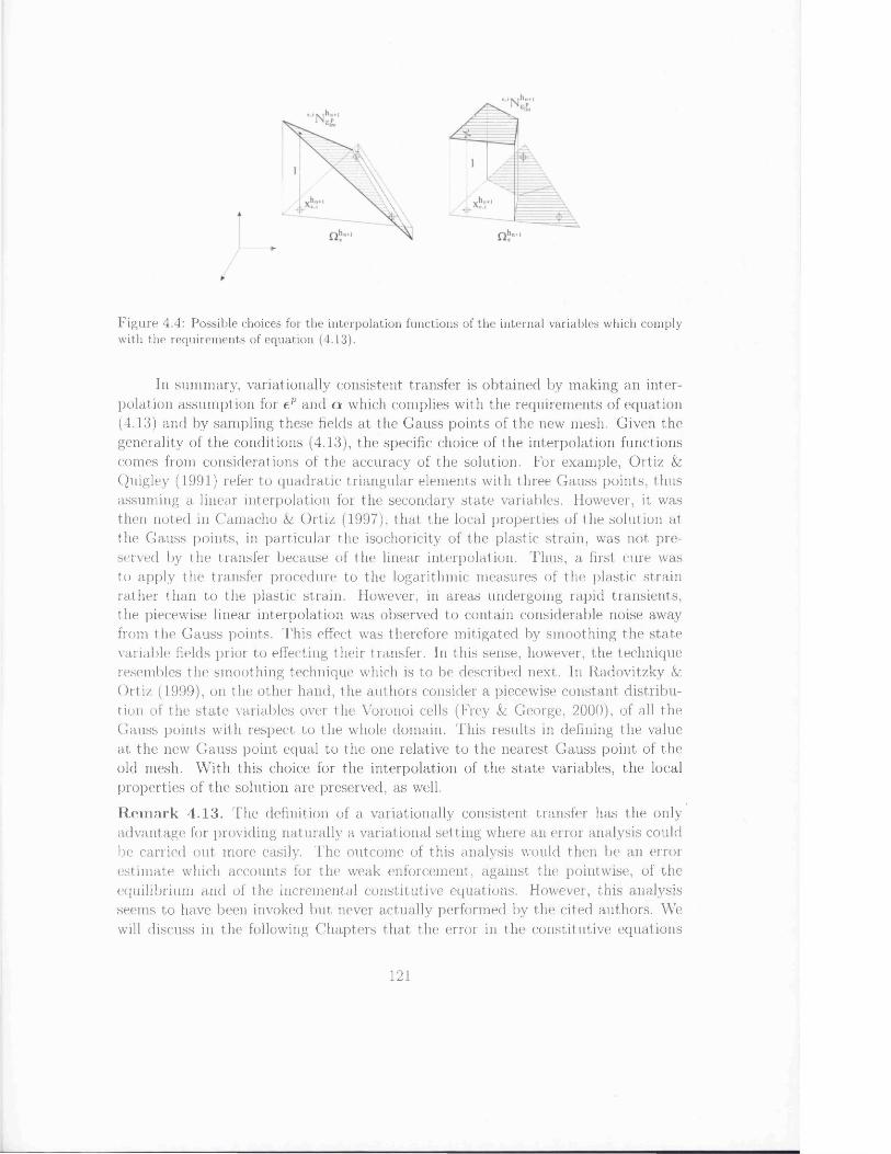
F igure 4.4: Possible choices for the interpolation functions of the internal variables which comply with the requirements of equation (4.13).

In summary, variationally consistent transfer is obtained by making an inter­polation assumption for ep and a which complies with the requirements of equation (4.13) and by sampling these fields at the Gauss points of the new mesh. Given the generality of the conditions (4.13), the specific choice of the interpolation functions comes from considerations of the accuracy of the solution. For example, Ortiz & Quigley (1991) refer to quadratic triangular elements with three Gauss points, thus assuming a linear interpolation for the secondary state variables. However, it was then noted in Camacho &; Ortiz (1997), that the local properties of the solution at the Gauss points, in particular the isochoricity of the plastic strain, was not pre­served by the transfer because of the linear interpolation. Thus, a first cure was to apply the transfer procedure to the logarithmic measures of the plastic strain rather than to the plastic strain. However, in areas undergoing rapid transients, the piecewise linear interpolation was observed to contain considerable noise away from the Gauss points. This effect was therefore mitigated by smoothing the state variable fields prior to effecting their transfer. In this sense, however, the technique resembles the smoothing technique which is to be described next. In Radovitzky & Ortiz (1999), on the other hand, the authors consider a piecewise constant distribu­tion of the state variables over the Voronoi cells (Frey & George, 2000), of all the Gauss points with respect to the whole domain. This results in defining the value at the new Gauss point equal to the one relative to the nearest Gauss point of the old mesh. With this choice for the interpolation of the state variables, the local properties of the solution are preserved, as well.

R em ark 4.13. The definition of a variationally consistent transfer has the only advantage for providing naturally a variational setting where an error analysis could be carried out more easily. The outcome of this analysis would then be an error estimate which accounts for the weak enforcement, against the pointwise, of the equilibrium and of the incremental constitutive equations. However, this analysis seems to have been invoked but never actually performed by the cited authors. We will discuss in the following Chapters that the error in the constitutive equations

121

will be able to account for the effects of the above approximations, in addition to the time discretization error in replacing the initial value constitutive problem with the incremental constitutive problem. In conclusion, it is worth noting that the definition of a variationally consistent transfer, by itself, does not guarantee that the most accurate adaptive finite element solution is delivered, as has been pointed out in the previous Section in the analysis of the heat conduction problem. □

4.5 .2 W eak enforcem ent o f th e continu ity

This transfer procedure is obtained from an approximation a la Galerkin of the variational equation which imposes in weak form the continuity across the time node tn of the variables which appear as data of the InBVP.

Let us assume, in the following, as general regularity property that (*)n G (L2(Q))ndim and also that (*)n G (L2(0 ))ndim, with equal to the number of components of the respective tensor field with respect to a given basis. The field (•)n is the data for the InBVP whereas (»)n is relative to the solution at the previous time interval.

The following condition

<W» - (•)», 0) = 0 , V0 e (L2(n))"“” (4.14)

enforces, in the weak form, the continuity of the field (*)n across the time node tn with {•, •) being an inner product for the space (L2 (Q))ndim.

In Rashid (2002), condition (4.14) is enforced in a Galerkin sense by replacing the infinite dimensional space (L2 (Q,))ndim with finite dimensional spaces defined by piecewise constant functions representing the distribution assumption for the variables and a£. These spaces are defined by constant functions over the Voronoi tessellation of each element with respect to its integration points and are denoted next with Chn and Chn+1 relative to T^n and Thn+1, respectively. If is the Voronoi cell relative to the point x G Q^n, the field hn€%(x), for instance, is defined as follows ngp

h' e l ( x ) = £ £ a „ ; , ( x ) '* ”eS (x^) n?nerh„ *=1

where 3 hn (cc) is the following function

and hnen(x eni) are the computed values from the solution at the previous time in­terval [£n_i, tn].

Likewise, the data field will be represented by

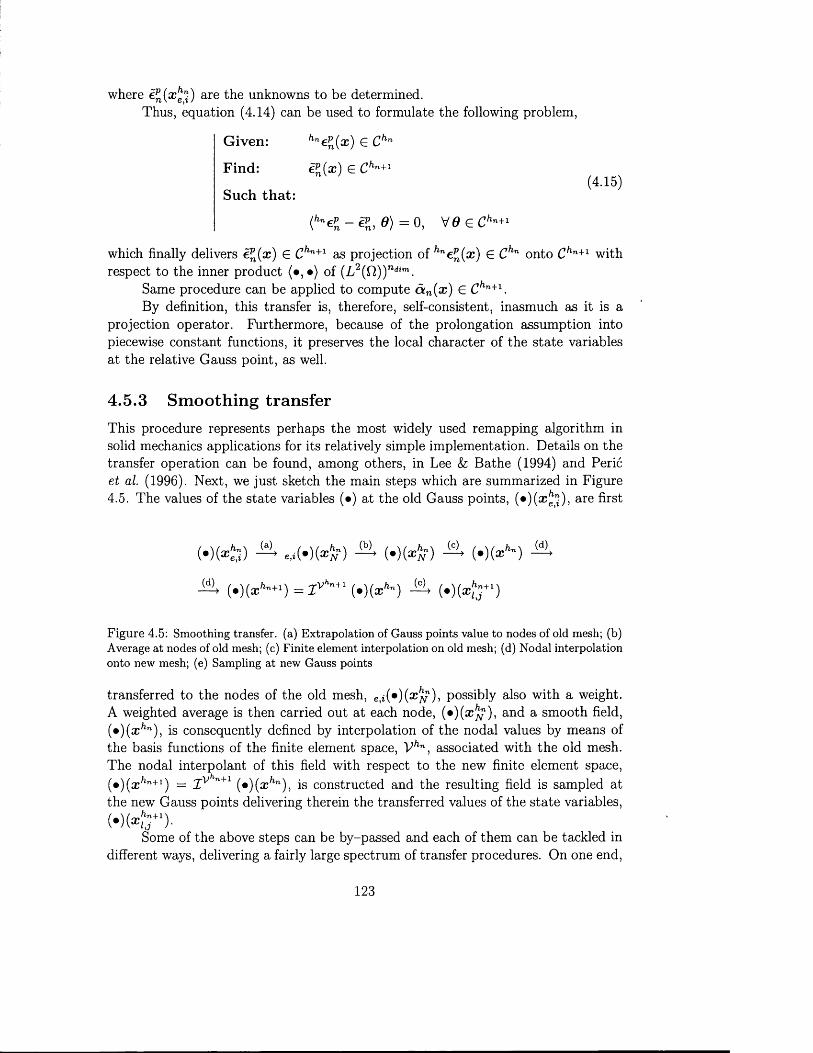
where e ^ ( x ^ ) are the unknowns to be determined.Thus, equation (4.14) can be used to formulate the following problem,

G iven: hnepn(x) G Chn

Find: e^(cc) G Chn+1(4.15)

Such that:

{hnepn - epn, 0) = 0 , V 0 e C hn+l

which finally delivers €.^(x) G Chn+l as projection of hne^(x) G Chn onto Chn+1 with respect to the inner product ( • ,• ) of (L2(Q))ndim.

Same procedure can be applied to compute 6cn(x) G Chn+1.By definition, this transfer is, therefore, self-consistent, inasmuch as it is a

projection operator. Furthermore, because of the prolongation assumption into piecewise constant functions, it preserves the local character of the state variables at the relative Gauss point, as well.

4 .5 .3 S m ooth in g transfer

This procedure represents perhaps the most widely used remapping algorithm in solid mechanics applications for its relatively simple implementation. Details on the transfer operation can be found, among others, in Lee & Bathe (1994) and Peric et al. (1996). Next, we just sketch the main steps which are summarized in Figure 4.5. The values of the state variables (•) at the old Gauss points, (•)(£Ee"), are first

(•)(*$!) ^ e » ( ^ ) ^ (• ) (* £ ) ^ (•)(**-) ^

(.)(x'*”« ) = i v‘"+i « (* * " ) (•) K r 1)

F igu re 4.5: Smoothing transfer, (a) Extrapolation of Gauss points value to nodes of old mesh; (b) Average a t nodes of old mesh; (c) Finite element interpolation on old mesh; (d) Nodal interpolation onto new mesh; (e) Sampling at new Gauss points

transferred to the nodes of the old mesh, e,i(9) ( x ^ ) , possibly also with a weight. A weighted average is then carried out at each node, (•)(# ^ 1), and a smooth field, (•){xhn), is consequently defined by interpolation of the nodal values by means of the basis functions of the finite element space, V^n, associated with the old mesh. The nodal interpolant of this field with respect to the new finite element space, (•) ( x hn+1) = Xv n+1 (•)(cc/ln), is constructed and the resulting field is sampled at the new Gauss points delivering therein the transferred values of the state variables,(•) (*JS+1).

Some of the above steps can be by-passed and each of them can be tackled in different ways, delivering a fairly large spectrum of transfer procedures. On one end,

123

there are those that obtain the values at the new Gauss points directly in terms of the values at the old Gauss points by means of interpolations which can be global or local over predefined neighbourhoods of the new Gauss points, such as in Tabbara et al. (1994); Boroomand & Zienkiewicz (1998) and Villon et al. (2000). On the other end, there are the procedures described in Figure 4.5, such as in Lee & Bathe (1994) and Peric et al. (1996). However, when the extrapolation to the nodes is considered, this represents a delicate point of the whole transfer process. Many studies have been carried out in the field of the so-called recovery procedures and various schemes such as least square fitting (Hinton &; Campbell, 1974), superconvergence-patch recovery (SPR) (Zienkiewicz & Zhu, 1992a), moving least square (Tabbara et al., 1994), etc. have been proposed. Despite its simplicity, the procedure however is not self-consistent and if frequent remeshing takes place diffusion of plastic strain can spread all over the domain because of the smoothing operation. Also, special care must be paid in accepting the transferred values. In fact, some properties can not be inherited by the values at the new Gauss points, namely the incompressibility of the plastic strain, for this constraint does not commute in general with the extrapolation operation.

R em ark 4.14. The previous classification is by no means exhaustive. A fairly general up-date account of current adaptive strategies in elastoplasticity can be found, however, in Ladeveze & Oden (1998). □

4.6 Numerical techniques. Newton-Raphson method

Without loss of generality and only for notational convenience, in the following we refer to the formulations of the discrete problems given in Section 4.4 rather than to problem (4.6), which is the one to be solved in an actual computation. Nevertheless, the considerations are general and can be easily adapted to (4.6).

The discrete problem (4.4), which here we formulate with generic data e£(x ), ctn{x), represents an algebraic system of nonlinear equations that is convenient to

124

write in the following form,

D ata : External Loading bn+i(x), on D,t n+i(x), on dQt

State of the system at t n

Find: u ^ X i i x ) G V^ 1

Such that: £(V.s«!rtT , Vh"+l ) =

el (x ) e £ a„(x) e A

(4.16)

■S (V .U & 1 (a )), V»A+1 (*))+

- ( b n+i{x),Tjhn+1(x)) - (tn+i(x) ,r jhn+1(x))dnt = 0

V77/ln+1 e Von+\

where the stress tensor /ln+1<Tn+i ( e ^ 1(::c) = ^ s u n+i(x ))i we recall, is the function of e^ 1 defined implicitly at any point x £ Q by the solution of the following problem with generic data e£(:r), d n(cc),

Data: e£, a n

G iven: e^ 1 = V a u J ^ a : )

F ind: /ln+1«£+i> hn+len+ \> hn+1otn +15 hn+lcrn+u hn+1A n+1

Such that: = hn+lef. ,, + hn+1epn + l n + 1 ' n + 1

'> - < T „ +1 = g ^ e ^ , ) ; ,‘" +M ( x , t „ +1) = a n+ 1)

hn+1 pP gP =±!-----2 6 3 f “+1cr„+1,'l'vHA>+1)

^ ‘a n+! - a „ e 0 (A„+1(rn+li/.«+1An+l)

(4.17)For the considerations of Section 4.4 we assume that problem (4.16) has solution for generic data e^(x),acn(x) as long as minimum regularity requirements are satisfied.

R em ark 4.15. The functional C = /^ (V s i i^ 1, rjhn+l) is defined over Vhn+1 x Vo"+1. However, next, whenever necessary, we will refer only to the dependence on 6y/ln + l _ □

There exist several techniques to solve the system (4.16) (Crisfield, 1991; Den­nis & Schnabel, 1996) which are mostly of iterative type. They, fundamentally, differentiate each other for their rate of convergence and for being locally or globally

125

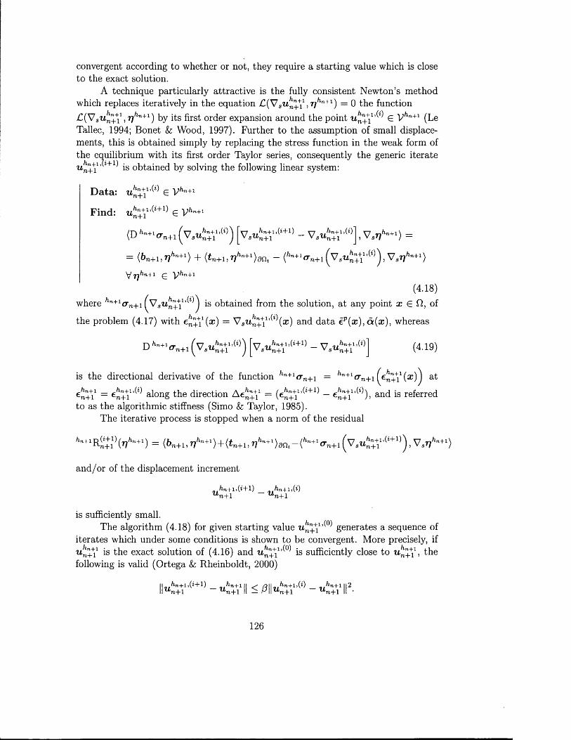
convergent according to whether or not, they require a starting value which is close to the exact solution.

A technique particularly attractive is the fully consistent Newton’s method which replaces iteratively in the equation £ ( V sujj+Y> r]hn+1) = 0 the function £ (V S ; Y , rjhn+1) by its first order expansion around the point w^+Y’ £ y^+ i (Le Tallec, 1994; Bonet & Wood, 1997). Further to the assumption of small displace­ments, this is obtained simply by replacing the stress function in the weak form of the equilibrium with its first order Taylor series, consequently the generic iterate u n+i1 is obtained by solving the following linear system:

D ata : Y’W 6 Vhn+1

Find: wJ+Y’(*+1) e

(D^'a-n+^V.u^,1’'0) [v,tt^V'(i+1) - V,t&Y'(0],V.V,“+') =

= <f>n+l,V*’'+1) + (*n+l>V‘”+1)dn, - (!'"+'Cn+1 ftsu 'n + l ’ V aV “+1)\ J r j h n+l £ y ^ n + 1

(4.18)where /ln+1crn+1 ^Vsi t „ + Y o b t a i n e d from the solution, at any point x € Cl, of

the problem (4.17) with = Vs'tt^Y ’ (x ) and data ep{x), 6t(x), whereas

d W B+1 (vs ;Y’(i)) [vs ;Y)(i+1) - v s ;Y’(i)] (4.19)

is the directional derivative of the function /ln+1<rn+1 = hn+1a n+i ^e^+Y(x )) at

€n+i = en+Y’ along the direction Ae^+Y — (en+Y’ +1 — 6n+Y’ )> an< referred to as the algorithmic stiffness (Simo & Taylor, 1985).

The iterative process is stopped when a norm of the residual

'‘”+1R|,7 iI)^ ' ,”+,) = (6«+i,'?'*”+,>+<tn+i,»?',"+,>a!),-< '‘“+V n+1( v su*;+1' ' (i+1)) ,V sT7',"+1>

and/or of the displacement increment

/ln+li(i+l) _ -.^n+lifi)u n+1 u n+1

is sufficiently small.The algorithm (4.18) for given starting value w£+Y’ generates a sequence of

iterates which under some conditions is shown to be convergent. More precisely, if ■u^Y ls tbe exact solution of (4.16) and w^+Y’ is sufficiently close to Y, the following is valid (Ortega &, Rheinboldt, 2000)

126

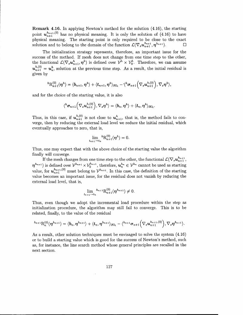
R em ark 4.16. In applying Newton’s method for the solution (4.16), the starting point w^+Y’ has no physical meaning. It is only the solution of (4.16) to have physical meaning. The starting point is only required to be close to the exact solution and to belong to the domain of the function £ (V su^+Y> ??/ln+1). □

The initialization strategy represents, therefore, an important issue for the success of the method. If mesh does not change from one time step to the other, the functional C (V su^+1,Tjh) is defined over Vh x Vq. Therefore, we can assume u n+i = solution at the previous time step. As a result, the initial residual is given by

h^ l i ( r i h) = (bn+i,V h) + <t„+i,V*W -•{Vn+i(v s« tf1)), v sr,h).

and for the choice of the starting value, it is also

V srjh) = (bn, 7]h) + (tn,rih)dnt-

Thus, in this case, if is not close to w£+1, that is, the method fails to con­verge, then by reducing the external load level we reduce the initial residual, which eventually approaches to zero, that is,

, lim ',Ri0j 1(V*)=0.tn+1 >n

Thus, one may expect that with the above choice of the starting value the algorithm finally will converge.

If the mesh changes from one time step to the other, the functional £ ( V sii£+Y j rjb-n+i) is defined over Vhn+l x Vo"+1, therefore, u^n E cannot be used as starting value, for u ^ Y ’ must belong to \?hn+1. In this case, the definition of the starting value becomes an important issue, for the residual does not vanish by reducing the external load level, that is,

lim '‘"+‘R£°j,(V‘"+‘) yt 0.* n + l

Thus, even though we adopt the incremental load procedure within the step as initialization procedure, the algorithm may still fail to converge. This is to be related, finally, to the value of the residual

(»?'*'•+■) = <bm ^ ' > + <tn , ^ ) a n , - (* ” + I<7„+i ,<0>) > V sVl'"+1)■

As a result, other solution techniques must be envisaged to solve the system (4.16) or to build a starting value which is good for the success of Newton’s method, such as, for instance, the line search method whose general principles are recalled in the next section.

127

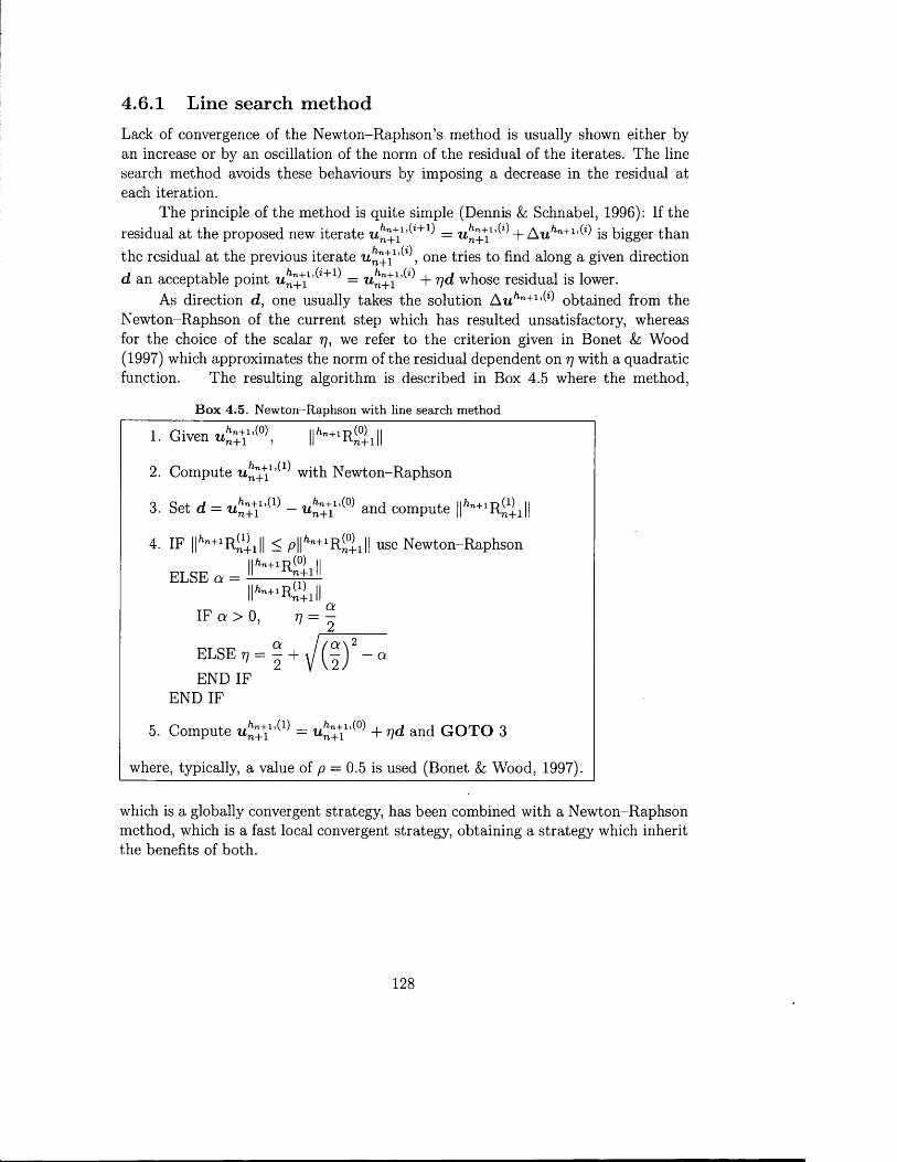
4.6.1 Line search m eth od

Lack of convergence of the Newton-Raphson’s method is usually shown either by an increase or by an oscillation of the norm of the residual of the iterates. The line search method avoids these behaviours by imposing a decrease in the residual at each iteration.

The principle of the method is quite simple (Dennis k, Schnabel, 1996): If the residual at the proposed new iterate = Wn+Y’ + A u /ln+1’ is bigger thanthe residual at the previous iterate u^+Y’ » one tries to find along a given direction d an acceptable point ^ n + 1.6 +1) = w^+Y’ + r]d whose residual is lower.

As direction d, one usually takes the solution A tt/ln+1’ obtained from the Newton-Raphson of the current step which has resulted unsatisfactory, whereas for the choice of the scalar 77, we refer to the criterion given in Bonet & Wood (1997) which approximates the norm of the residual dependent on 77 with a quadratic function. The resulting algorithm is described in Box 4.5 where the method,

END IF END IF

5. Compute mJ[+Y’ = u n + i ' ^ + and G O T O 3

where, typically, a value of p = 0.5 is used (Bonet & Wood, 1997).

which is a globally convergent strategy, has been combined with a Newton-Raphson method, which is a fast local convergent strategy, obtaining a strategy which inherit the benefits of both.

B ox 4.5. Newton-Raphson with line search m ethod

1. Given f - i e i l

2 . Compute u^+Y’ with Newton-Raphson

3. Set d = u hnX l1,(1) - u hn+Y’(0) and compute H ^ R i + J

4. IF ||/ln+1R^1 ^ i+ i l l use Newton-Raphson

ELSE a -

IF a > 0, 77 = -

ELSE 77

128

4.7 Concluding RemarksIn this Chapter we have described the displacement finite element solution of an elastoplastic model with internal variables discretized in time with the backward Euler method. A critical analysis of the nature of the discretization errors introduced in the formulation of the fully discrete scheme has been provided. In particular, the fundamental observation has been made that change of data and/or finite element mesh from one time interval to the other can be both related to a discontinuity jump of the approximate solution across the time instant tn. Also, a critical review of the current techniques to transfer of the data from one mesh to the other has been given.

However, before proceeding to the study of the transfer procedures in terms of the error produced, in the next Chapter we will first consider how to use the extended dissipation error to assess the quality of finite element solutions with meshes constant throughout the loading process. The objective is to show that this error measure is able to account for effects of time and space discretization error, and also to provide the relative importance of the error components associated with the residual in the state law and in the evolution law.

129

Chapter 5

The error in the constitutive equations to assess the quality of the finite elem ent solution w ith mesh c o n s t a n t in tim e

5.1 IntroductionObjective of this chapter is the application of the general theory of the error in the constitutive equations developed in Chapter 3 to the assessment of the quality of finite element solutions of elastoplasticity problems.

The general properties of an admissible solution of the problem under consid­eration have been given and discussed in Section 3.5. For instance, with respect to the computation of the extended dissipation error, an admissible solution is the set of the time dependent fields of the state variables which satisfy the compatibility and equilibrium equations along with the initial conditions. As a result, a finite element solution obtained for instance by a displacement formulation, is not in general an admissible solution. The values are discrete in time and the finite element stresses do not satisfy the equilibrium equations in a pointwise manner.

In order to apply the theory of the error in the constitutive equations, given the finite element solution, a corresponding admissible solution must be therefore defined. However, if the admissible solution must reflect the approximations asso­ciated with the finite element solution, it is understood that some conditions are necessary for its definition (Ladeveze h Pelle, 2001). A rather general one can be expressed in the following terms

Given a family of finite element solutions which converges to the exact solution as the discretization parameters approach their corresponding limit values, then also the family of corre­sponding admissible solutions converges to the exact solution and possibly with the same rate of convergence.

130

In linear elasticity, this condition refers to the definition of the so called prolon­gation conditions, that is, to the conditions posed on the definition of the statically admissible stress fields in terms of the computed finite element stresses, so that the error in the constitutive equation can be bounded above by the exact error in solu­tion. A thorough analysis of the meaning of this condition can be found in Ladeveze & Leguillon (1983) and Ladeveze & Pelle (2001) for the constant triangular element and is referred to as strong prolongation condition.

In this chapter, the finite element mesh is assumed to be constant throughout the time evolution of the continuum. As a result, the admissible solution correspond­ing to the finite element solution will be time continuous. Criteria to build a such admissible solution for the computation of the extended dissipation error are first given in general and then detailed for the Prandtl-Reuss model. Numerical analysis of its performance compared to classical measures of the error are illustrated on a ID model problem. In the second part of the chapter, we recall also the dissipation error and compare its performance to the extended dissipation error.

5.2 Extended Dissipation ErrorIn the definition of an admissible solution for the computation of the extended dissipation error, the statically admissible variables are not constrained to their conjugate variables by means of the state laws as it happens in the dissipation error. This allows more information from the finite element solution to be included in building the corresponding admissible solution and strengthen the link between the two solutions. For example, in the case of a ,/2-plasticity model and of finite element solution which delivers plastic strains meeting the incompressibility condition, the computed plastic strain field can be assumed, in some circumstances, as part of the admissible solution. In particular, in a displacement finite element formulation the plastic strain, known only at the Gauss points of the element used forthe numerical integration of the constitutive equations, can be extended over the element in a field which continues to meet the incompressibility condition. This can be realized, for example, by assuming each element partitioned by the Voronoi cells associated with each Gauss point and assuming a constant distribution of the plastic strain over the cell equal to the value of the strain at the respective Gauss point. In this way we define a plastic strain field whose incompressibility is guaranteed at almost every point of the domain. For elements with only one Gauss point, the field will be clearly constant over the element. Figure 5.1 depicts, for instance, the definition of the Voronoi cells for the triangular element when one or three Gauss points are used for the numerical integration of the constitutive equations, respectively, along with the assumed distribution of internal variables. Clearly, one can envisage also other partitions of the element along with relative definition of the state variables distribution. It will follow that the error in the constitutive equations will have to be considered as the error associated with the given assumption for the state variables distribution.

131

/1 Gauss Point 3 Gauss Points

Figure 5.1: P artition of a triangular element with Voronoi cells relative to its Gauss points along with respective assumed distribution for the internal variables

Likewise, conforming finite element displacements can be used as part of the admissible solution and do not need to be modified, unlike for the definition of the admissible solution to compute the dissipation error, as it will be discussed in the following (Moes, 1996).

A key feature of the analysis and implementation of the error in the consti­tutive equations, however, is in general the definition of an equilibrated stress field <7ad{x,tn+1) linked to the finite element solution hcrn+i ( x ^i). A substantial body of research has been devoted to recover more or less equilibrated stress field on the basis of the computed finite element stresses such as in Stein & Ahmand (1977), Zienkiewicz &; Zhu (1992c), Ainsworth & Oden (1993), Wiberg et al. (1994) and de Miranda & Umbertini (2002), among others. In these works different condi­tions are given to relate the recovered stress field to the finite element stresses. In the following we refer to the techniques initiated by Ladeveze (1975) where the so called prolongation condition depending in general on the regularity of the mesh establishes the aforementioned link (see, e.g., Ladeveze, 1994; Ladeveze Sz Pelle, 2001). In particular, hereafter, we apply the strong prolongation condition as intro­duced and analysed in Ladeveze (1975), Ladeveze & Leguillon (1983) and Ladeveze & Pelle (2001). This condition distinguishes the statically admissible stress fields °rad(^, tn+1) which satisfy the following equation for every shape function Ni(cc) and for all the elements

J (<rad{x, tn+i) - ha n+i{x)^j : VNi(sc)dft = 0 . (5.1)

For anisotropic meshes, the condition (5.1) is required to hold for any element Qe and for any shape function of higher order which is associated with a non vertex node. This condition has been termed as weak prolongation condition in Ladeveze (1994) and Ladeveze & Rougeot (1997).

The only unknowns left apart and necessary to determine a complete admis-

132

sible solution are, therefore,

P a d { ^ t ra+l)> d a d ip t - t ^n+l) >

^ad(®)^n+l)j X.ad{?C) ^n+l)•

For their computation, the general method of minimization of the error introduced in Ladeveze et al. (1999) can be adopted. However, in general, it may be much more convenient to resort to the simpler criterion given in Ladeveze h Moes (1997) which resembles the integration of the evolution law for the constitutive model which is used. Next, we detail this construction for the Prandtl-Reuss model.

5.2.1 C on struction o f th e adm issib le so lu tion

Plasticity M odel P I: Prandtl Reuss M odel w ith Linear HardeningThe essential equations for this model are hereafter recalled, cf. Section 3.2.4.5,

Yield Condition: II^SlI - {Rad + Ro) < 0, Rad > 0

Rad; eead, P ad) = (cTad - C e ^ : C_1 ('(Tad - +

+ ( Rad - HPad) H-1 ( Rad - Hpad'j ;

W x ^ a d , Rad; ePad, pad) = R0 ||e^ || - (Tad ■ e£d + RadPad,

with Tr[e^d] = 0 and pad > 11^11 > where \\q\\ = y/q : q is the norm of the second order tensor q.

In the following, we refer to the solution of a fully implicit conforming finite element displacement formulation of the initial boundary value problem of the plas­ticity model under consideration. The primary variable is given at the discrete time instants tn+i in terms of the finite element displacement field u„+l(x), whereas the secondary variables, such as ha n+i, he^+1, hpn+15 are issued only at the Gauss points

used for the numerical quadrature of the internal virtual work. As a result of the considerations of Section 4.2, we recall that on conceptual level, all the secondary variables can be obtained at any point x G Q provided that at this point and for all the previous discrete time instants tn, the incremental constitutive value problem has been solved. This would require to store the computed finite element displace­ment field at each discrete time instant tn and consequently huge memory capacities would be necessary. By contrast, in an incremental solution procedure, only the accepted solution at the previous discrete time instant is stored at most. The stress field which would be so obtained would not satisfy anyway the equilibrium equations in a pointwise manner, thus the finite element solution cannot be used to compute the extended dissipation error.

Objective of this section is to propose a procedure to build an admissible solution corresponding as close as possible to the computed finite element solution and make use of minimum memory requirements. This is feasible because equation (3.48) shows that the extended dissipation error at the time tn+1 can be expressed

133

in terms of only the error at the time tn and the admissible solution over [in, tn+1]. As a result, the admissible solution can be defined in an incremental manner, as well. Consistently with an assumed linear variation of the external load over each time interval and the convexity of the equilibrium and compatibility conditions, the admissible solution is taken to vary linearly over [tn, £n+i]. Therefore for its complete definition we need to solve the following problem

G iven: the admissible solution at tn,the finite element solution at tn+1,

F ind: a corresponding admissible solution at tn+\.

As far as the definition of the admissible displacement field and the equilibrated stress field are concerned, the general considerations given in the previous section apply. In particular, the equilibrated stress field is obtained with a two-stage pro­cedure. The first consists, by means of the prolongation condition, in defining an equilibrated traction forces along the boundary of each element and the second in solving the equilibrium equations over each element, usually, with higher order el­ements. For technical details we refer to Rougeot (1989), Ladeveze et al. (1991), Ladeveze & Rougeot (1997) and Ladeveze h Pelle (2001). The outcome is the defi­nition of a statically admissible stress field crad { x , tn+1), which is known at any point x E Q and is continuous over Q.

Also, we consider hereafter the computed finite element plastic strain to be extended over the domain with the criterion given in the previous section so that it makes sense to write hepn+l{x) for each x 6 Cl. For the definition of other admissi­ble state variables epd( x , t n+1), Pad(x,tn+i), Rad{x, tn+1) we start from the general procedure indicated by Ladeveze et al. (1999), which considers the minimization of the extended dissipation error over the set of the admissible values for the re­maining state variables. The minimization can be carried out at each point of the domain since there are no spatial derivative involved in the constitutive equations, in particular it will be done at the Gauss points used to compute numerically the space integrals that define the error (cf. Ladeveze & Pelle, 2001). These quadrature points do not have to be confused with those where the constitutive equations are in­tegrated numerically. These points in turn are the one used to compute numerically the integral that appear in the internal virtual power.

The minimization problem in its general terms is described in Box 5.1. An approximate solution of this problem can be obtained as follows. We assume the admissible thermodynamic force R ad{x, tn+i) given by

Radix, tn+1) = Max {Ri, R 2}

where

#1 = \WadiX ^ n + l ) \ \ ~ Ro

R 2 — Radix^tn).

134

Box 5.1. Definition of the state variables as minimization of the extended dissipation error

For each x £ tt

G iven: &ad(.X) in), Radip^i t n ) ,

^-adi& i in), ^n ) ’ P ad ip^ i tn)-

i n + l ) , ^-adi^i i n + l )

Find: R ad(xi i n + l ) ,

ead(* ’ in+l), Vadip^i tn+ l)

such that by assuming a time linear variation over [in, t n+1] of the vari­ables

G’adi.X, t)) Fad{x^ i ) ,

ead(x , t ) , epad(x , t ) ,pad{ x , t ),

we realize the minimum of the following function

F((Jad, R adi ^adi -adi Pad) —

= supf-1

: C- l <Tad{x, t ) - C €ead{ x , t )

+

+

<Tad{x,t) - Ceead(x, t)

Rad{x,t) - Hpad(x, t) H_1 Rad(x, t) - Hpad(x, t)

Ro\\£Pad(x , T)\\ -<Tad(x,r): epad(x , r ) + Rad(x,T)pad(x,T)

+

+

/ d r

under the following constraints

Ik S fo O II - (Rad(x,t) + R 0) < 0,

Pad(x,t) > \\epad{ x , t ) l

V t e [ in, in+i] t)} = 0

ead{x,t) = eead(x, t) + epad(x , t )

Rad{x,t) non-negative and non-decreasing

135

The admissible plastic strain, on the other hand, will be given by

ePad(X >tn+1) = /l<+l(®)

if the following condition is satisfied,

crad( x , t n+1): [hepn+l(x) - epad( x , t n)\ >0 .

Otherwise we choose

(5.2)

<«iOMn+l) =Finally, with regard to the admissible accumulated plastic strain p ad( x , t n+1)

it isPad{x i t n+ 1) — P a d { x , t n ) + j | , ra+l) Caci(*C’^0 ||

which corresponds to the integration of the equation p = \Kd\\ that occurs for the model under consideration by assuming linear variation of the variables over[tni ^n+l]‘

Condition (5.2), which represents the discrete implicit expression of the plastic power, can be interpreted in the light of the minimization of only the pointwise contribution to the error in the evolution law, 6d, within the time interval [tn, tn+1], given by

[tn,tn+i]Cd(®)=f [ [floll€pad( x , r ) \ \ - a ad(x, r) : epad(x, r) + Rad(x, T)pad(x, r)Jtn 1

under the constraints

T)] = °> P a d (x , r) > \\epad(x, t )

d r

(5.3)

(5.4)

Further to the assumption of linear variation of the variables which enter into(5.3), and by accounting for (5.4), after some rearrangements, it also follows

7 5 II A P II &ad{X-> tn+l) T 0 ’a d ( * ^ , tn) A p . Rad(x, tn-\-1) T Rad{.X,tn)^ollA e^J------------------ : Ae£d + ----------------------------------Apad >

> I I Mad I Ro + R a d i x , tn+l) \\cradiX ^tn+l)\\'fl(xD { x , t n-^i): TIA€p (x) +

+ |f lQ + R ad( x , t n) - ||<r^(a,£n) | |n ^ ( c c , in): n A€Pad(x)

where we have let

= tn+1 ) ~ ^ a d (X i ^n )> ^ P a d = P adijX , £n+l) — P a d {x , tn)

and

<?ad{xit) = \ \<r^(x, t) \ \naD ( x , t ) , A e pad{x) = \\Aepad{x) \ \nAePad{x).

136

Finite lower bounds for the function (5.3) can therefore be obtained by the minimization of the expression

ad I2

Ro + Rad(x,tn+1) - \\(T d( x , t n+i)\\n(rDd( x , t n+1): n Aep^(x) . (5.5)

However, by inspection, we note that lower values of this function correspond to Ae^d such that

n aDd( x , tn+1) : n AePad > 0. (5.6)

By choosing the admissible plastic strain e^d( x , t n+1) as described above we respect both condition Tr[Ae£d] = 0 and (5.6), and also we include information pertinent to the finite element plastic strain.

Once all the admissible state variables have been computed at tn+1, the use of a time linear interpolation over [tn, £n+i] guarantees the admissibility of the solution for the convexity of the equilibrium and compatibility conditions. Also, the above procedure delivers an admissible solution which produces a finite value of the error for the convexity of the domains E and C introduced in Section 3.2.4.5.

R em ark 5.1. The use of a time linear interpolation of the computed nodal values has the implied assumption that the accuracy of this time dependent function is thesame as the computed nodal values. This is not the case in general but it holds forsmall values of the time step At. □

External Loads at L External Loads at Ln bn bn+lL tn+1

FE Solution at L FE Solution at t„+iul? u t ,ha„ hCTn+ihe? heR+ihP„ hP*ryH

rh *. % tnH %Uad(*») Uad(/n+l)°ad On) °ad (fn+1)Ead(/n) Ead (tn+i)Pad('") Pad (*n+1)

Adm Solution at tn Adm Solution at tn+i

F igu re 5.2: Finite element solution and admissible solution for finite element mesh Th constant in time.

Figure 5.2 reports schematically the notation relative to the finite element solutions and corresponding admissible solutions in the case of finite element mesh constant in time.

137

5.2.2 Error E xpressions

In the section Error Analysis which follows, comparisons of the extended dissipation error with classical measures of the exact error in solution will be reported. The aim is to illustrate that the extended dissipation error reflects quite well the evolution of the admissible solution with respect to the exact one as described by more classical measures of the error. This section therefore presents the expressions of the classical measures of the error used for the subsequent numerical comparison and recalls, for the reader’s convenience, the expressions of the extended dissipation error and the error in solution.

Classical m easures o f the exact error in so lu t ionAs shown in the previous section, the extended dissipation error applied to the finite element solution measures actually the accuracy of an admissible solution corre­sponding to the finite element solution. The admissible solution is a time dependent function which is obtained as time linear interpolation of the discrete values at the time instants used for the time discretization of the initial boundary value problem under consideration. Thus, it is this time dependent solution that will be assumed in the definition of the exact error. Furthermore, as generalization of the error in elasticity, it has been observed in Section 3.5.3 that the extended dissipation error can be interpreted as a global measure of the error of the kinematically admissible solution skJ = (eady epad, pad)- Thus, it appears quite natural to consider the L°°L2 norm of the exact error of the admissible total strain,

lL°°([0,T];(L2(n))dxd) = SUP \\e£ad(x,t)\\(L2 (njjdxd ='Cad I

= MAX SUP < / U ex(x, t) - ead(x, t)) : (eex(x, t) - ead(x, t)) d x i , i<n<Nte[tn,tn+i] [Jn J

along with the L°° control in time of the free complementary energy norm of the exact error of the generalised stress field conjugate of the kinematically admissible solution. That is, if we let

\\ed-(x, t)\\v — f {<Tex{x,t) - Ceead{ x , t ) ) : C_1 (o-ex(aj,0 - Ceead{x , t)) dx Jn

IIeR(X>t)\\M= ReX{x, t) - H p ad(x, t) H R ex{x, t) - Hpad{x, t) J n L J L

then, it follows

II^gsf||loo([o,t];VxA/1) = SUP { ||e*(x, t ) III + ||e^(® ,£)||^} 5 .

This choice is motivated by the following result T heo rem 5.1.

dx

138

Given a kinematically admissible solution s ^ n = iead, €pd, Pad)>

■adip i t) = Z-exix, 0

lle e | |L oo([0,T];(L2(O))dx d) = 0 £ a d (X > 0 ~ € ex(X ^ )=* V x e n V* < T

l | e GSFlU~([0,T];Vx.M) = 0 f) = £ Pi (X i ()

P a d ( x , t ) = p ex(x, t)The proof follows by the same arguments as in the proof of Theorem 3.9, and

will not be repeated here.

Error in the constitutive equationsThis error measure is given by equation (3.47) which is here rewritten in a form that fits better the incremental origin of the admissible solution sad = i^ad, Rad ] Cad, £PadiVad)-

eL.cn =*(«)

MAX SUP \ f ( a U x ^ - C e ^ t ) ) : - Ce'ad(x , t ) )d x +1 < n < N te[ tn , tn+i] I / q

+ / [Rad( x , t ) - H p ad(x,t)]H 1[Rad(x, t) - Hpad(x , t ) \d x +Jn

+ »2(<„) + 2 j J R o | | £ ^ ( a : , r ) | | - < T „ d ( x , r ) : £ j j ( x , r ) + ^ ( x . r j p ^ x . r ) d r d x >,

(5.7)where

^d(^n) = 2 [ f \ R o\\ePad(x , *)ll “ a ad{x, t) : epad(x, t) -f floras, t)Pad(x, t) Jo Jfl 1

dxdt .

Equation (5.7) basically expresses the global error at the time T in terms of the error at time tn and of the admissible solution over [tn, T}.

Since the admissible solution sad( x , t ) is continuous piecewise linear over each time step, the time integral in the error expression can be computed easily. Hence, we have for t 6 [tn, tn+1],

In It ~~ < ? a d { x , T ) : epad{x,T) + R a d i x , T)pad{x ,T)}dr d x =’n J t

t — tz - f { r o | |a £^ (x ;' Ln Jfl k

& a d i x , i ) T & a d { x , t n )

+

t n+l un Jfl

Radix, t'j + Radi x , in)

: Aead(®) +

&Padix)}dx

139

where

A e a d ( X ) = e?a d ( X > * n + l ) “ *n)

A P a d ( * ~ V a d i p ^ i t n + l ) P a d { X - > ^n)>

whereas a ad(x, t) and R ad( x , t ) are the time linear interpolation over [£n, £n+i] of the respective values at tn and £n+i. Also, it follows

= £ 2 [ ^ ( * ) +i = l L 2

+ f i a J ( x , f i+1) + f l a, ( x , <i) A p a d , ( a ; ) | d a .

with

A e P a d , i ( X ) = ePa d ( X ^ i + 1) - < £ * (* > * 0

A Pad,i{X ) = Padip^i ^i+l) Padip^i i)'

The value of the dissipation error at U = 0, 6d(ti), assumed equal to zero.

E rror in solutionThis error measure is given by equation (3.74) which is the extended dissipation error associated with the admissible solution seXiad = (crex, R ex ; e ad , e pd , p ad).

elx(T ) =

= MAX SUP I [ (aex{ x , t ) - C e ead{x, t)): C 1 (crex{x, t) - Ceead{x, t)) dx +l<n<N te[tn,tn+i} \ Jn '

+ f [Rex(x, t ) - Hpad{x, t)] H-1 [Rex(x, t ) - Hpad(x, t)]dx + 92d ex(tn) + (5.8)Jfi

I fJ J tn+ 2 /?0 ||6 ^ (a 3 ,r ) || - crex( x , r ) : epad(x,T) + R ex(x ,T )p ad( x , r ) d r d x } ,

where, as before, it is

elex(tn) = 2 [ [ \Ro\\epad{x,t)W - ( T ex(x, t): epad(x , t ) + R ex(x, t)pad{x, t)Jo Jfl 1

dx dt.

Unlike the analogous expression (5.7), crex(x , t ) and Rex(x, t), as functions of time, are not in general linear over each time step, therefore the time integral must be computed by accounting for the actual time variation of the functions.

140

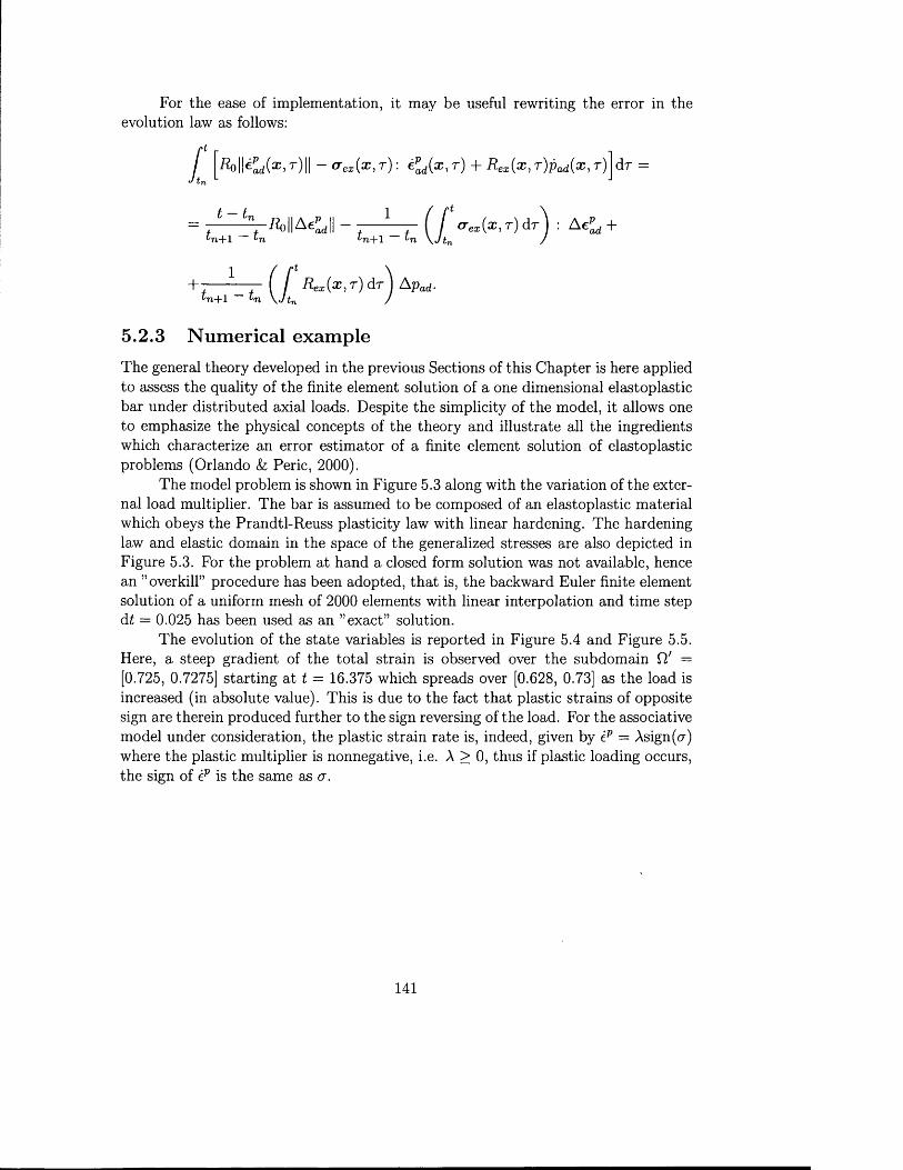
For the ease of implementation, it may be useful rewriting the error in the evolution law as follows:

flolKd(*>T)ll - a ex(x ,r) : epd(x, r ) + R ex{x, r)pad(x, r)

V ^ o l l Aeadll - t— l— r ( f <rex{x,T)dT\ : A epad + t n + l t n \ J t n /

d r =

t — t^ 7 ) 4 - 1

+■'/n+1

]- j - R ex{x,r) d r^ Apad.

5.2 .3 N u m erical exam ple

The general theory developed in the previous Sections of this Chapter is here applied to assess the quality of the finite element solution of a one dimensional elastoplastic bar under distributed axial loads. Despite the simplicity of the model, it allows one to emphasize the physical concepts of the theory and illustrate all the ingredients which characterize an error estimator of a finite element solution of elastoplastic problems (Orlando & Peric, 2000).

The model problem is shown in Figure 5.3 along with the variation of the exter­nal load multiplier. The bar is assumed to be composed of an elastoplastic material which obeys the Prandtl-Reuss plasticity law with linear hardening. The hardening law and elastic domain in the space of the generalized stresses are also depicted in Figure 5.3. For the problem at hand a closed form solution was not available, hence an ’’overkill” procedure has been adopted, that is, the backward Euler finite element solution of a uniform mesh of 2 0 0 0 elements with linear interpolation and time step dt = 0.025 has been used as an ’’exact” solution.

The evolution of the state variables is reported in Figure 5.4 and Figure 5.5. Here, a steep gradient of the total strain is observed over the subdomain Q' = [0.725, 0.7275] starting at t = 16.375 which spreads over [0.628, 0.73] as the load is increased (in absolute value). This is due to the fact that plastic strains of opposite sign are therein produced further to the sign reversing of the load. For the associative model under consideration, the plastic strain rate is, indeed, given by ep = Asign(cr) where the plastic multiplier is nonnegative, i.e. A > 0, thus if plastic loading occurs, the sign of ep is the same as a.

141

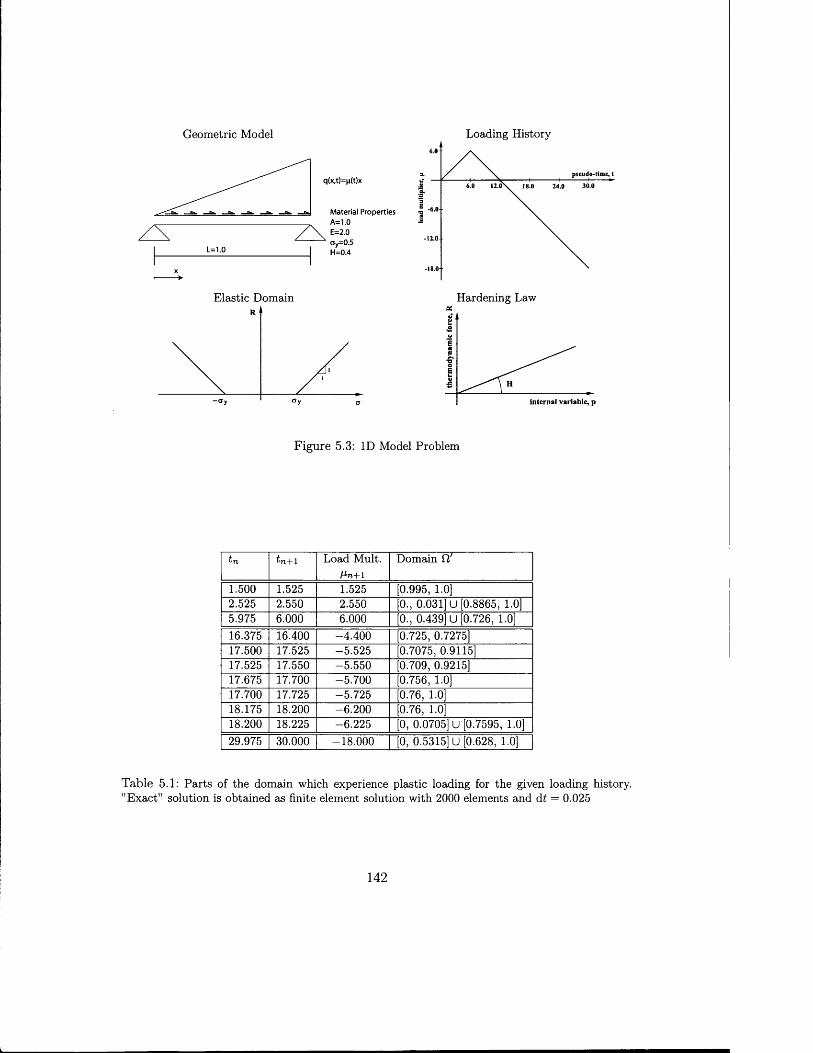
Geometric Model Loading History

q(x,t)=p(t)x

Material PropertiesA=1.0E=2.0Oy—0.5H=0.4

p s e u d o - t im e , t

Elastic Domain Hardening Law

internal variable, p

F igure 5.3: ID Model Problem

tn tn+1 Load Mult.I^n+l

Domain fI'

1.500 1.525 1.525 [0.995, 1.0]2.525 2.550 2.550 [0., 0.031] U [0.8865, 1.0]5.975 6 .0 0 0 6 .0 0 0 [0., 0.439] U [0.726, 1.0]16.375 16.400 -4.400 [0.725, 0.7275]17.500 17.525 -5.525 [0.7075, 0.9115]17.525 17.550 -5.550 [0.709, 0.9215]17.675 17.700 -5.700 [0.756, 1.0]17.700 17.725 -5.725 [0.76, 1.0]18.175 18.200 - 6 .2 0 0 [0.76, 1.0]18.200 18.225 -6.225 [0, 0.0705] U [0.7595, 1.0]29.975 30.000 -18.000 [0, 0.5315] U [0.628, 1.0]

T able 5.1: P arts of the domain which experience plastic loading for the given loading history. ’’E xact” solution is obtained as finite element solution with 2000 elements and d t — 0.025

142

L

Exact Stress Distribution Exact Total Strain Distribution1 5

1

0 5

0

•1•15-2 Space Domain

•........— —

:—

i 0.1 0.2 o.3 0 4 o s 0 6 o!r\'o"i vb>.......V > \ \ \

\ \ \ \ X ‘\ \ \ \ ^

-------- 1=0 75 v o , \ ............ 1=1.5 \ \ \ ^

1=225 \ \ \1=30 \ \ ’i

.......... 1=3 75 \ \1=4 5 V. >

.............. 1=5-25----- 1=6.0

1=675

Exact Stress Distribution

_ ....................:i 0 1 0.2 o.3 0 4 o.5 o - ; o - 8 . . o:d

W : ; ;-------- t=6 75.......... 1=7 5

1=8 25 1=9 0

--------t=9 75------ 1=10 5

1=11.25-------- 1=12.0

t=12 75

Exact Total Strain Distribution2

1

0

-2

-3

-4

-5 Space Domain

I

*=13 5 t= 14 25 1*15.0 1=15 75 1*16.5 1=17 25 1=180 1= 18 75

151

0 5

0-05

-1■15-2

-25

-3

-3.5

1=22.5 1=23 25 1=24 0 1=24 75

5

4

3

213

0

-2-3

1=24.75 1=255 1=26 25 1=27.0 1=27.75 1=285 1=29 25 *=30 0

10

8

64

20-2

-4

-6 Space Domain

F igure 5.4: Exact Stress and Total Strain Distribution at each d t = 0.75 for t € [0 .0 , 30.0]

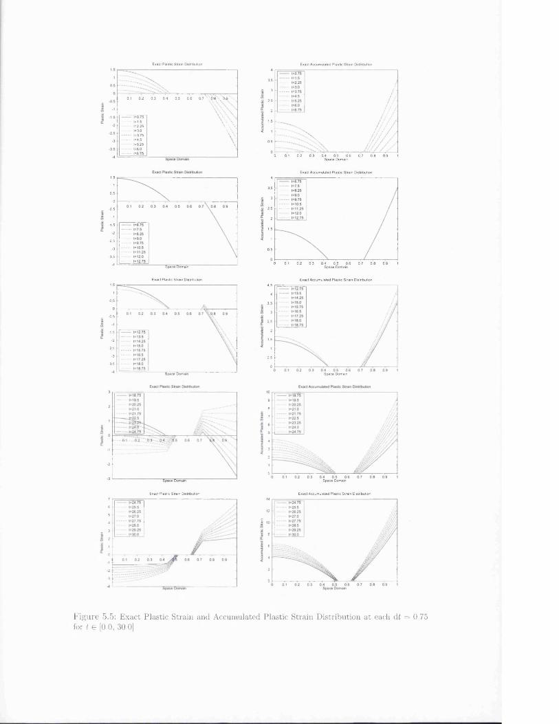
Exact Plastic Strain Distribution

0 1 0 2 0 3 0.4 0 5 0 6 0 7 \ 0 ? 8 \ W ' N

\ \ \\ \ **'

\ \

V\

-------- 1=0.75.......... t=1 5

1=2.25 1=3 0

-------- 1=3 75------ 1=4 5

1=5.25t=601=6.75

Exact Accumulated Plastic Strain Distribution

3 5

3

2.5

215

0.5

00 0 1 0.2 0.3 0 4 0.5 0.6 0 7 0.8 0 9Space Domain

1.5

10 5

0-0.5

-1■1.5

•2-2 5

-3

-3 5

-4 Space Domain

Exact Accumulated Plastic Strain Distribution4

3 5

3

2 5

21.5

10 5

00 0.1 0 2 0.3 0.4 0 5 0 6Space Domain

0 7 0 8 0 9 1

Exact Plastic Strain Distribution Exact Accumulated Plastic Strain Distribution1.5

10 5

0-0 5

■1 5

-2-2 5

-3

-3 5

Space Domain

4 5

4

3 5

3

2 5

21 5

0 5

0Space Domain

Space Domain

109

87

4

3

2

0Space Domain

Exact Plastic Strain Distribution Exact Accumulated Plastic Strain Distribution7

65

4

3

210■1-2-3

-4

I

14

12

8

6

4

20

F igu re 5.5: Exact Plastic Strain and Accumulated Plastic Strain Distribution a t each d t = 0.75 for t e [0.0, 30.0]

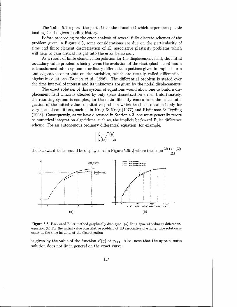
The Table 5.1 reports the parts ST of the domain Q which experience plastic loading for the given loading history.

Before proceeding to the error analysis of several fully discrete schemes of the problem given in Figure 5.3, some considerations are due on the particularity of time and finite element discretization of ID associative plasticity problems which will help to gain critical insight into the error behaviour.

As a result of finite element interpolation for the displacement field, the initial boundary value problem which governs the evolution of the elastoplastic continuum is transformed into a system of ordinary differential equations given in implicit form and algebraic constraints on the variables, which are usually called differential- algebraic equations (Brenan et al, 1996). The differential problem is stated over the time interval of interest and its unknowns are given by the nodal displacements.

The exact solution of this system of equations would allow one to build a dis­placement field which is affected by only space discretization error. Unfortunately, the resulting system is complex, for the main difficulty comes from the exact inte­gration of the initial value constitutive problem which has been obtained only for very special conditions, such as in Krieg & Krieg (1977) and Ristinmaa & Tryding (1993). Consequently, as we have discussed in Section 4.3, one must generally resort to numerical integration algorithms, such as, the implicit backward Euler difference scheme. For an autonomous ordinary differential equation, for example,

V = F(y) y(to) = yo

the backward Euler would be displayed as in Figure 5.6(a) where the slope ——

Appr. Solution corr. to A/* Appr. Solution corr. to A/"

(a)

F igu re 5.6: Backward Euler method graphically displayed: (a) For a general ordinary differential equation (b) For the initial value constitutive problem of ID associative plasticity. The solution is exact at the time instants of the discretization

is given by the value of the function F{y) at yn+\. Also, note that the approximate solution does not lie in general on the exact curve.

145

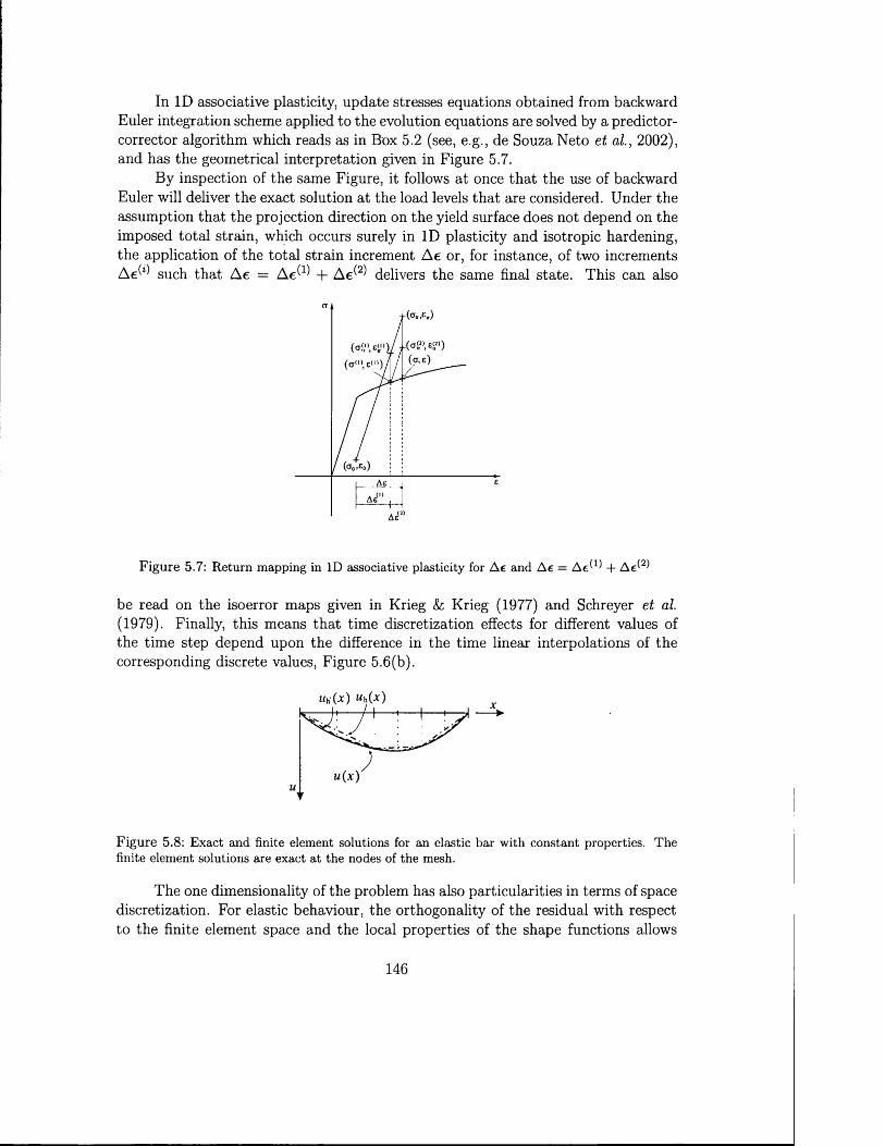
In ID associative plasticity, update stresses equations obtained from backward Euler integration scheme applied to the evolution equations are solved by a predictor- corrector algorithm which reads as in Box 5.2 (see, e.g., de Souza Neto et al., 2002), and has the geometrical interpretation given in Figure 5.7.

By inspection of the same Figure, it follows at once that the use of backward Euler will deliver the exact solution at the load levels that are considered. Under the assumption that the projection direction on the yield surface does not depend on the imposed total strain, which occurs surely in ID plasticity and isotropic hardening, the application of the total strain increment Ae or, for instance, of two increments A e^ such that Ae = A e ^ + A e ^ delivers the same final state. This can also

A e'

F igu re 5.7: Return mapping in ID associative plasticity for Ae and Ae = A e ^ + A e ^

be read on the isoerror maps given in Krieg & Krieg (1977) and Schreyer et al. (1979). Finally, this means that time discretization effects for different values of the time step depend upon the difference in the time linear interpolations of the corresponding discrete values, Figure 5.6(b).

u(x)

F igu re 5.8: Exact and finite element solutions for an elastic bar with constant properties. The finite element solutions are exact a t the nodes of the mesh.

The one dimensionality of the problem has also particularities in terms of space discretization. For elastic behaviour, the orthogonality of the residual with respect to the finite element space and the local properties of the shape functions allows

146

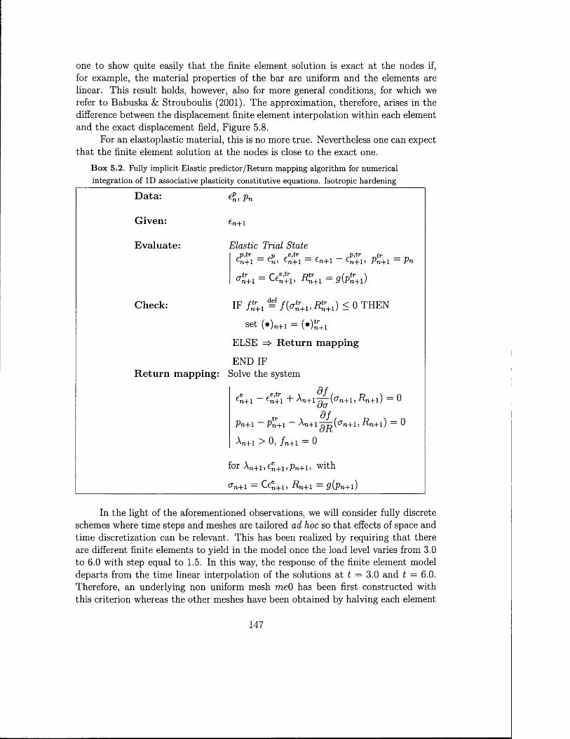
one to show quite easily that the finite element solution is exact at the nodes if, for example, the material properties of the bar are uniform and the elements are linear. This result holds, however, also for more general conditions, for which we refer to Babuska & Strouboulis (2001). The approximation, therefore, arises in the difference between the displacement finite element interpolation within each element and the exact displacement field, Figure 5.8.

For an elastoplastic material, this is no more true. Nevertheless one can expect that the finite element solution at the nodes is close to the exact one.

B ox 5.2. Fully implicit Elastic predictor/R eturn mapping algorithm for numerical integration of ID associative plasticity constitutive equations. Isotropic hardening

Data:

Given:

Evaluate:

C Pn

€n+l

Elastic Trial Statep . t r n e . t r p . t r t r

^n+l > n+1 €n+1 ^n+l > Pn+1 Pn

CT,JT+1 = Ce'-y,, /& .! = < ? (* ,)

Check: I F fS+1 = f W r+ 1 . R ‘n + i ) < 0 THEN

set (•)„+! = ( • ) ^ +1

ELSE => R eturn mapping

END IFR eturn mapping: Solve the system

,e ,tr d f€n+1 ~ €n+1 + An+i ^ ( a „ +i, R n + l) ~ 0

^ J'

Pn+1 ~ Pn+l ~ 777 (crn+1> ^7i+l) = 0d R

^ 7 i+ l 0 ) f n + 1 0

for An+i,e*+1,pn+i, with

71+1 - 71+1) - 71+1 9{Pn+l)

In the light of the aforementioned observations, we will consider fully discrete schemes where time steps and meshes are tailored ad hoc so that effects of space and time discretization can be relevant. This has been realized by requiring that there are different finite elements to yield in the model once the load level varies from 3.0 to 6.0 with step equal to 1.5. In this way, the response of the finite element model departs from the time linear interpolation of the solutions at t = 3.0 and t = 6.0. Therefore, an underlying non uniform mesh me0 has been first constructed with this criterion whereas the other meshes have been obtained by halving each element

147

' I +-*■ * I"

I lHHWHHWIWIH Hl|

meO 7 els

met 14 els

mei 56 els

6.0 -

pseudo-time, t

30.018.0 24.06.0 12.1

-6.0 - -

-12.0 - -

-18.0 —

F igu re 5.9: Fully discrete schemes analysed

of the corresponding parent mesh. Also, uniform partition of the time interval of interest with time steps k = A t = 6.0, 3.0, 1.5, 0.75 have been assumed. The fully discrete schemes are shown in Figure 5.9. These have been analysed using an incremental solution based on the backward Euler stepping scheme and the Newton- Raphson procedure. Only one Gauss point has been used for the integration of the constitutive equations, because linear finite elements are used. Plastic strain he^+1 and accumulated plastic strain hpn+i, obtained at the single quadrature point of each element, are prolongated into uniform field over the respective element.

For the definition of the corresponding admissible solution necessary to com­pute the extended dissipation error the criteria described in the previous Section apply. In particular, if the ID system is statically indeterminated, the statically admissible stress field crad(^, tn+i) is obtained by solving over each element G the following equilibrium problem,

Vf i J = } x he, X he + i [ e %

- - j ^ d O M n + i ) + f { x , t n+l) - ° (5 .9 )

F**1 u dNh f x*+'v ead(x e>t n+ i) = - a ( x ) { x ) dx + f (x, £n+i)Ne (x) dx

J x h dx J x h

where the boundary condition is obtained from the prolongation condition (cf. Ladeveze h Leguillon, 1983)

J h (< f(M n + i) - ha{x)^jv{x)dx V . G V W (5.10)

with V/l(Dg) being the finite dimensional space generated by the element Lagrangian shape functions Ng(a;) and Ng+1 (x) depicted in Figure 5.10.

148

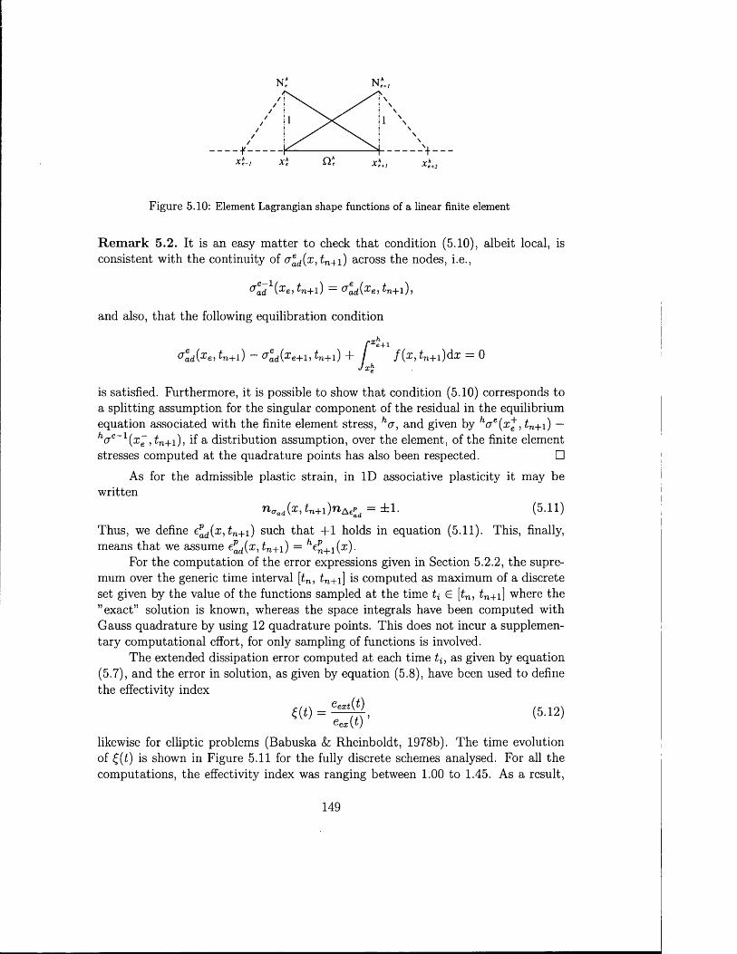
N* N*+/

////

F igu re 5.10: Element Lagrangian shape functions of a linear finite element

R em ark 5.2. It is an easy matter to check that condition (5.10), albeit local, is consistent with the continuity of ald(x, tn+1 ) across the nodes, i.e.,

< d 1(Ze,£n+1) = (Jead{xe, t n+1),

and also, that the following equilibration condition

f Xe+1o ead(xe, tn+i) - a ead{xe+1, tn+1) + / f{x, tn+i)dx = 0

J

is satisfied. Furthermore, it is possible to show that condition (5.10) corresponds to a splitting assumption for the singular component of the residual in the equilibrium equation associated with the finite element stress, hcr, and given by ha e(x* , tn+1 ) — ha e~1(x~, £„+i), if a distribution assumption, over the element, of the finite element stresses computed at the quadrature points has also been respected. □

As for the admissible plastic strain, in ID associative plasticity it may be written

n aad{x, tn+i)nAePd = ±1. (5.11)

Thus, we define e d(x , tn+1 ) such that +1 holds in equation (5.11). This, finally, means that we assume eJdOMn+i) = M + iW -

For the computation of the error expressions given in Section 5.2.2, the supre- mum over the generic time interval [£n, £n+i] is computed as maximum of a discrete set given by the value of the functions sampled at the time U E [£n, £n+i] where the ” exact” solution is known, whereas the space integrals have been computed with Gauss quadrature by using 12 quadrature points. This does not incur a supplemen­tary computational effort, for only sampling of functions is involved.

The extended dissipation error computed at each time £*, as given by equation(5.7), and the error in solution, as given by equation (5.8), have been used to define the effectivity index

m = (5.i2)€ex\L)

likewise for elliptic problems (Babuska & Rheinboldt, 1978b). The time evolution of £(£) is shown in Figure 5.11 for the fully discrete schemes analysed. For all the computations, the effectivity index was ranging between 1.00 to 1.45. As a result,

149

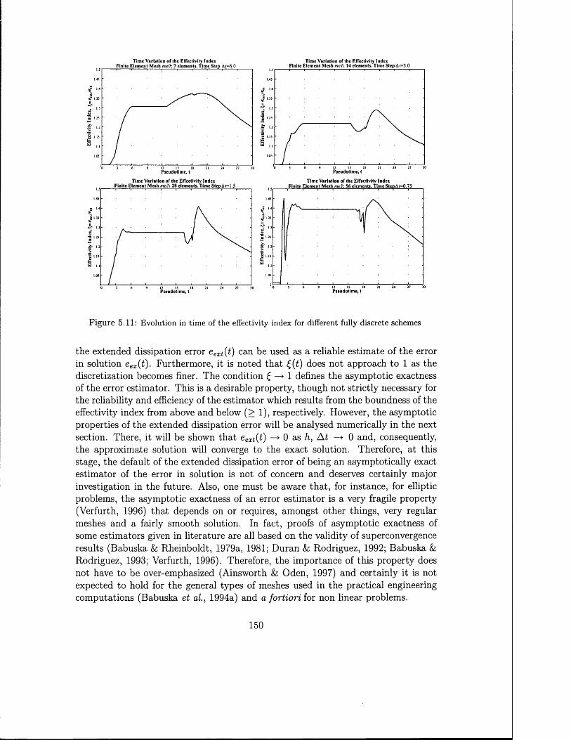
Tim e Variation o f the Effectivity IndexFinite E lem ent iviesn m ev: / elem ents. I im e step Ar=6.0

\

2 1>

I 'hi

Pseudotim e, t

Tim e Variation o f the Effectivity IndexFinite Elem ent iviesn m e/: m elem ents. n m e» tep A f= 1 .5

isf*oa

shiPseudotim e, t

F igu re 5.11: Evolution in time of the effec

the extended dissipation error eexi{t) ca] in solution eex(t). Furthermore, it is nol discretization becomes finer. The condit of the error estimator. This is a desirable the reliability and efficiency of the estirm effectivity index from above and below ('. properties of the extended dissipation er section. There, it will be shown that ee; the approximate solution will converge stage, the default of the extended dissip* estimator of the error in solution is no investigation in the future. Also, one m problems, the asymptotic exactness of a (Verfurth, 1996) that depends on or re meshes and a fairly smooth solution, some estimators given in literature are a results (Babuska &; Rheinboldt, 1979a, 1 Rodriguez, 1993; Verfurth, 1996). Ther< not have to be over-emphasized (Ainswi expected to hold for the general types ( computations (Babuska et al., 1994a) ar

Tim e Variation o f the Effectivity Index Finite Elem ent M esh m e/: 14 elem ents. Tim e Step Ar=3.0

■oQ

£

Pseudotim e, t

T im e Variation o f the Effectivity IndexFinite Elem ent M esh meS: 56 elem ents, l im e Ste^Af=0.7S

TJB

££

Pseudotim e, t

ivity index for different fully discrete schemes

. be used as a reliable estimate of the error ed that £(£) does not approach to 1 as the on £ —> 1 defines the asymptotic exactness property, though not strictly necessary for

tor which results from the boundness of the > 1), respectively. However, the asymptotic or will be analysed numerically in the next t{t) —> 0 as h, At —> 0 and, consequently, to the exact solution. Therefore, at this tion error of being an asymptotically exact ; of concern and deserves certainly major ist be aware that, for instance, for elliptic i error estimator is a very fragile property plires, amongst other things, very regular ’n fact, proofs of asymptotic exactness of 1 based on the validity of superconvergence 981; Duran h Rodriguez, 1992; Babuska & fore, the importance of this property does >rth & Oden, 1997) and certainly it is not f meshes used in the practical engineering d a fortiori for non linear problems.

150

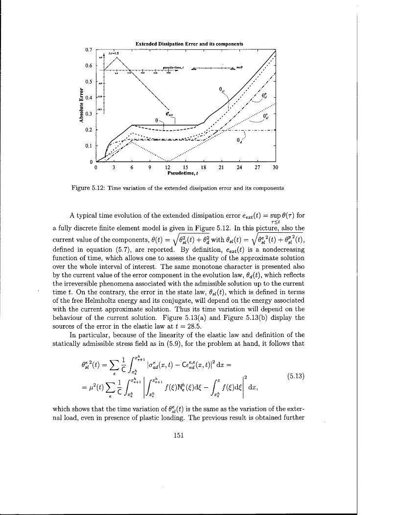
Extended Dissipation Error and its com ponents0.7

0.6 pseudo-lime, /

0.5

0.4

0.3

0.2

0.1

0300 3 6 9 12 15 18 21 24 27

Pseudotim e, t

F igu re 5.12: Time variation of the extended dissipation error and its components

A typical time evolution of the extended dissipation error eext(t) = sup^(r) forT<t

a fully discrete finite element model is given in Figure 5.12. In this picture, also the

current value of the components, 0{t) = y j o 2s l{ t) + 6% with 6si(t) = y J + ^ ( t ) , defined in equation (5.7), are reported. By definition, eext(t) is a nondecreasing function of time, which allows one to assess the quality of the approximate solution over the whole interval of interest. The same monotone character is presented also by the current value of the error component in the evolution law, 6d{t), which reflects the irreversible phenomena associated with the admissible solution up to the current time t. On the contrary, the error in the state law, 0si(t), which is defined in terms of the free Helmholtz energy and its conjugate, will depend on the energy associated with the current approximate solution. Thus its time variation will depend on the behaviour of the current solution. Figure 5.13(a) and Figure 5.13(b) display the sources of the error in the elastic law at t = 28.5.

In particular, because of the linearity of the elastic law and definition of the statically admissible stress field as in (5.9), for the problem at hand, it follows that

I rhe + 1

I - G%(x, t) |2dx =(5.13)

which shows that the time variation of 6esl (t) is the same as the variation of the exter­nal load, even in presence of plastic loading. The previous result is obtained further

151

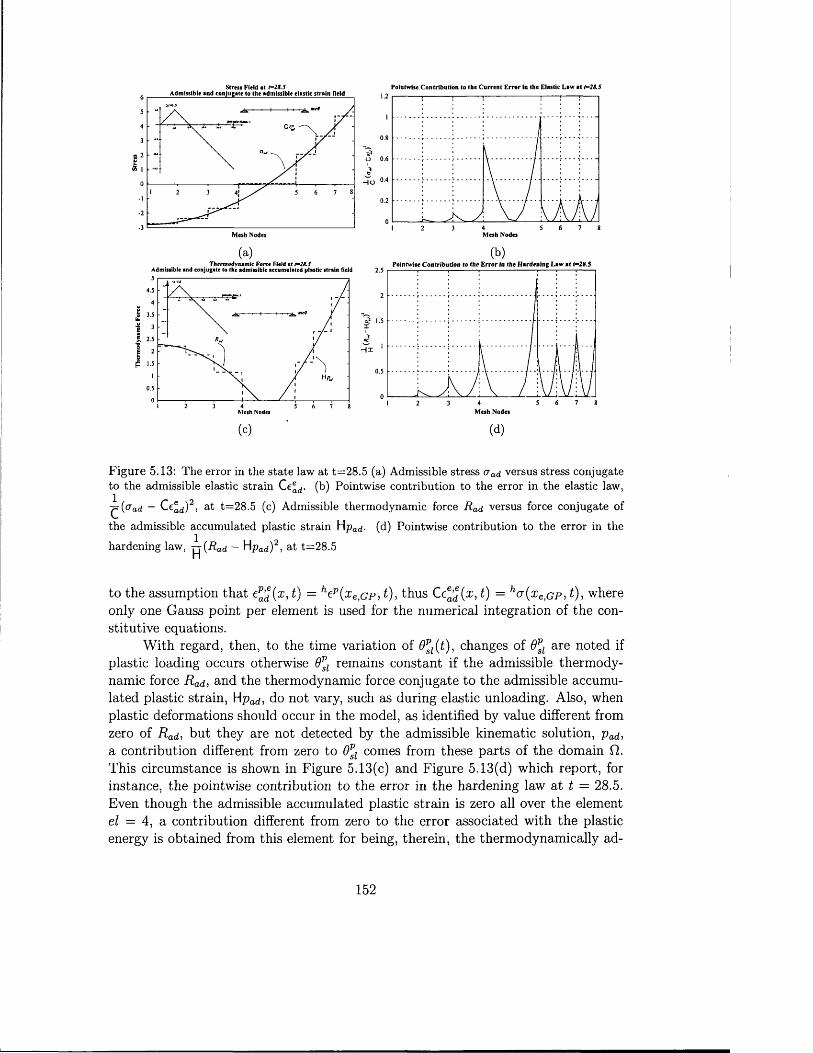
Admissible »nd conjugate to the admissible e listic strain field65

4

3

2

Ho0

■2•3

Mesh Nodes

Pointwise Contribution to the Current Error In the Elastic Law at t=28.51.2

0.8

0.6

0.4

0.2

3 40 6 7 852

Mesh Nodes

(b)Thermodynamic Force Field at t=28.5

Admissible and conjugate to the admissible accumulated plastic strain field5

4.5

4

3.5

3

2.5

21.5

0.5

0 2 3 54 7 86

Po in tw ite Contribution to the Error in the Hardening Law at t=28.52.5

2

1.5

0.5

0Mesh Nodes

(c)Mesh Nodes

(d)

F igu re 5.13: The error in the state law at t=28.5 (a) Admissible stress a ad versus stress conjugate to the admissible elastic strain Ce®d. (b) Pointwise contribution to the error in the elastic law,

Q ^ad ~ C6®d)2, a t t=28.5 (c) Admissible therm odynamic force R ad versus force conjugate of

the admissible accumulated plastic strain Hpad- (d) Pointwise contribution to the error in the

hardening law, j j ( R ad — Hpad)2, at t=28.5

to the assumption that cp’d{x> t ) = hep(xe cp, t), thus Ce^(x, t ) = hcr(xeiGP, £), where only one Gauss point per element is used for the numerical integration of the con­stitutive equations.

With regard, then, to the time variation of 9psl(t), changes of 0psl are noted if plastic loading occurs otherwise 9psl remains constant if the admissible thermody­namic force R ad, and the thermodynamic force conjugate to the admissible accumu­lated plastic strain, Hpad, do not vary, such as during elastic unloading. Also, when plastic deformations should occur in the model, as identified by value different from zero of R ad, but they are not detected by the admissible kinematic solution, pad, a contribution different from zero to 6psl comes from these parts of the domain Q. This circumstance is shown in Figure 5.13(c) and Figure 5.13(d) which report, for instance, the pointwise contribution to the error in the hardening law at t = 28.5. Even though the admissible accumulated plastic strain is zero all over the element el = 4, a contribution different from zero to the error associated with the plastic energy is obtained from this element for being, therein, the thermodynamically ad­

152

missible force different from zero. This may be interpreted as the plastic energy that we have somehow to supply to this part of the domain, since the kinematically admissible solution was not able to describe it.

Major critical insight in the causes that produce variation of the error in the evolution law, Qd, is obtained by analysing the pointwise contribution to 9d within a given time interval [tn, tn+1],

\tn,tn+1]£(x) = f [#o||c£d(a;, £)II -crad(x, t): epad{x, t) + R ad{x, t)pad{x, £)] dt Jtn

which is next considered in its general tensorial notation.By accounting for the definition of the admissible plastic strain and accumu­

lated plastic strain, the assumption of time linear variation for the admissible solu­tion over the time interval [tn, £n+i] and the fact that n aD (®, £): n&€Pd(x) = +1, it follows that

[tn,tn+l\Cd ( X ) —

+

IIAead IH o + R a d (*E, i n + l ) l l ^ a d (* ® » ^ n + 1 ,

Rq T Hacj(®, tn) ||(Jad( x , tn)

+(5.14)

where, in general, Ho + Radix, t) - \\(Tad{x,t)\\ > 0.As a result, if at the point x 6 Q the following expressions are valid

Ho + Radix, tn) - \\(T d{x , tn)\\ = 0 ,

Ho + Radix, fn+l) II adiX> in+l) || = 0,

then there is no local contribution to the error in the evolution law from the current time interval. This, in turn, means that given

D („ +\ £)adt) =

R a d i x , t ) —

i n + l i n

t tni n + l I nt — L

( ® , t n + l ) +

R a d i x , i n + l ) +

t n —l i

i n + l i n

in— 1 i in+1 in

in—i i

<7adiX i in)

Radixj in)

P a d i x , t )

i n + l i nt — t

i n + l i n

i n + l i nA - P a d i x , £n + i ) + t n 1

i n + l i n

^adiX> tn)

Padix, in)

(5.15)

with\\(T°dix, tn) || - (H0 + Radix, £„)) < 0

\\<T°dix, £n+l)|| - (Ho + Radix, tn+l)) < o

Tr[A6^ ] = 0

a Pad = IIAeJJJ

n a D< ( x , t ) : n Aep (x) = + 1 , V£ e [tn, t n+i]

(5.16)

153

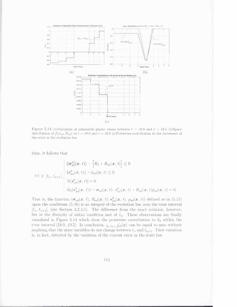
(a)

e.1<

Mesh Nodes

Space Distribution of fftfjj.R jj) = lo«it -(R * j+ a y)

■8

1 2 3 4 7 85 6

(b)0.018

0.016

0.014

0.012

0.01

0.008

0.006

0.004

0.002

0 2 3 4Mesh Nodes

5 6 7 8

(c)

F igu re 5.14: (a)Variation of admissible plastic strain between t = 18.0 and t = 19.5 (b)Space distribution of f(crad-, -Rad) at t = 18.0 and t = 19.5 (c)Pointwise contribution to the increment of the error in the evolution law.

then, it follows that

V t e [tn, £n + i ] ,

I I - R o + R a d ix , t) < 0

U Pad(X i O i l -Pad{x, t ) < 0

T r& la h 01 = 0

R o U Pad(X ’ O i l “ a ad{x, t): ePad( x , t) + Rad{x, t)pad( x , t) = 0.

That is, the function [aad{x, t), Rad{ x , t)\ £pad{x, t), pad (x , t)) defined as in (5.15) upon the conditions (5.16) is an integral of the evolution law over the time interval [£n, £n+i], (see Section 3.2.4.5). The difference from the exact solution, however, lies in the diversity of initial condition met at tn . These observations are finally visualized in Figure 5.14 which show the pointwise contribution to 6d within the time interval [18.0, 19.5]. In conclusion, [tn,tn+1](d{x) can be equal to zero without implying that the state variables do not change between tn and tn+\. Their variation is, in fact, detected by the variation of the current error in the state law.

154

R atio o f C u rre n t E r ro r C om ponen ts to the E r ro r as S u prcm umE xtended D issipation E rro r and its com ponents Finite E lem ent M esh m el: 14 elements. T im e S fepA / = 3 .0 — 0

01 /eexi0.9

0.8

0.7

10.6^ 0.4

% 0.5

* 0.4

0.3

0.2

0.1

00 3 6 9 12Pseudorim e,

15 I Pseudotim e, t

18 21 24 27 30 21 24 27 300 3 6 9 12 18

R atio of C u rren t F.rror C om ponents to the E r ro r as S uprem tExtended D issipation E r ro r and its com ponents Finite E lem ent M esh m e l : 14 elem ents. T im e Step A I = 1.5

0.80.5

w 0.4

0.4

0.2

00 3 6 9 12Pseudotim e, t

15 18 21 24 27 30 27 3012 15 21 240 3 6 9 IXR atio o f C u r re n t F .rro r C om p o n en ts to the Ei

Finite E lem ent M esh m e l : 14 elem ents. T im e step At= 0.750.7

0.6

0.5

u 0 .4

0.3

0.2

0.1

00 3 9 15 8 21 24 27 306 21 24 27 30

F igure 5.15: Extended dissipation error along with its components for different discretizations. Evolution of the error in the state law and in the evolution law with respect to the global error as the time step is reduced.

5.2.4 Analysis o f the error

In this Section the behaviour of the extended dissipation error with respect to the parameters that control the approximation, namely time step size and mesh size, is investigated numerically. We start by analysing the relative importance of the error components 9si arid 9d with respect to the global error eext.

Figure 5.15 describes the influence of the time discretization for a given finite element mesh, which is the mesh m el defined in Figure 5.9, whereas Figure 5.16 shows the influence of the space discretization for given time discretization realized by uniform time step A t = 1.5. In general, one notes a reduction of the absolute error eext along with the variation of the relative importance of its components.

155

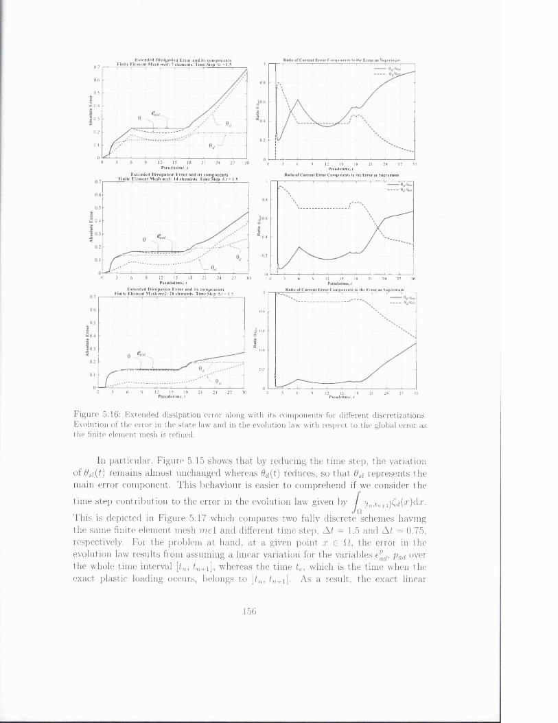
E xtended D issipation E rro r and its com ponents Finite E lem ent M esh meO\ 7 elem ents. Time Step At =1.5

Components to the Ei Suprcmum

0.7

0.6

0.5

£ 0.4

30.3<0.2

0.1

00 3 6 9 12 15P scudotim e, t

18 21 24 27 30 0 96 12> 15Pscudotime,

21 2418 27 30

E xtended D issipation E rro r and its com ponents F inite E lem ent M esh m e l: 14 elem ents. T im e Step A t = 1.5

Components to the Error as SupremiI

Ui 0.4

0.4

0.2

00 3 96 12Pscudotim e,

15P seudotim e, t

2118 24 27 30 30 9 12 156 18 21 24 27 30

Extended D issipation E r ro r and its com ponents F inite E lem ent M esh me2: 28 elem ents. T im e Step A/ = 1.5

Components to the Ei Suprcmum

0.8

J 0.65.

0,4

0.2

00 3 6 9 12 15Pscudotim e, i

18t 21 24 27 30 0 6 9 12 27! 15 IPseudotime, t

21 24 30

F igure 5.16: Extended dissipation error along with its components for different discretizations. Evolution of the error in the state law and in the evolution law with respect to the global error as the finite element mesh is refined.

Iii particular, Figure 5.15 shows that by reducing the time step, the variation of 0si(t) remains almost unchanged whereas Qd{t) reduces, so that 0si represents the main error component. This behaviour is easier to comprehend if we consider the

time step contribution to the error in the evolution law given by / [fnifn+1]C(i(a:)da:.

This is depicted in Figure 5.17 which compares two fully discrete schemes having the same finite element mesh m el and different time step, A t = 1.5 and A t = 0.75, respectively. For the problem at hand, at a given point x E fl, the error in the evolution law results from assuming a linear variation for the variables e^d, pa<i over the whole time interval [tn, £n+1], whereas the time tc, which is the time when the exact plastic loading occurs, belongs to \tn, £n+i[- As a result, the exact linear

156

T im e Step C o n tr ib u tio n to th e E r ro r in the E vo lu tion Lai _________F in ite E lem en t M esh mel: 14 e le m e n ts ._________

T im e Step At=1.5 Tim e Step At=0.75

0.04

0.02

3 15 300 9 12 18 24 276 21P seudo tim e, t

(a)

E x ten d ed D issipa tion E r r o r a n d its co m p o n en ts F in ite E lem en t M esh m e l: 14 e lem en ts . T im e S tep A I = 1.5

E x ten d ed D issipa tion E r r o r an d its c o m p o n en ts F in ite E lem en t M esh m e l : 14 e lem en ts . T im e s te p A i= 0.750.7 0.7

0.6 0.6

0.5 0.5

u 0.4 u 0.4

0.3 0.3.a<0.2 0.2

0.1

021 24 12 15 21 24 27 300 3 6 9 12 15 18 27 30 0 183 6 9I’seu d o tiin e , I

(b)

F igure 5.17: Contribution to the error in the evolution law for given finite element mesh, m el, and different time discretizations, time step A t = 1.5 and At = 0.75 (a) Time step contribution to the error in the evolution law (b) Time variation for the extended dissipation error along with its components

tn

fn+Af" fn+2A<" /n + 3A/'' t„ + 4At"

F igure 5.18: Effect of the time step on the error in the evolution law for different time discretiza­tions At, A t', At", with At = 2A t' and A t' = 2A t"

157

variation of ep and p occurs only over [tc, tn+1].The reduction of the time step reduces the time interval during which the plas­

tic flow contributes to the error because of the linear interpolation. This situation is sketched in Figure 5.18.

Figure 5.16, as well, shows that by refining the finite element mesh size the error component Osi(t) reduces drastically so that 8d constitutes the main error component. The dependence of 8si on the mesh size h, and more specifically of 6esi on h, can also be revealed by a direct analysis of the equation (5.13). Figure 5.16 also shows that the dependence of Qd on the mesh size is not well defined as it can be inferred from comparing the variation of Qd for the meshes meO and m el. Here, it is noted that dd increases by refining the mesh size. This behaviour is visualized in Figure 5.19 which compares the time step contribution to the global error in the evolution law for the previous schemes. This circumstance occurs as a result of alarger area experiencing plastic loading detected by the mesh m el with the elementsel = 7 and el = 8 , as shown in Figure 5.20.

Another aspect taken into account in this section is to motivate the use of the extended dissipation error by showing that this measure of the error does indeed reflect the global quality of an admissible solution. This is proved numerically on the model problem under consideration by investigating the behaviour of the family of finite element approximations corresponding to values of the discretization parameters approaching their limit values, that is,

e-ext 0 as h, A t —> 0

&ext ^ext,At h ► 0 (5.17)

&ext &ext,h <S At ► 0

where eext^ t and eext^ denote the error due to only time and space discretization, respectively. That is, eexttAt is defined as the error associated with the exact solution of the nonlinear incremental boundary value problem obtained by performing only the time discretization of the initial boundary value problem; whereas, eext,h is the error associated with the exact solution of the system of differential algebraic equations obtained by performing only the space finite element discretization of the initial boundary value problem.

We also compare the time evolution of the extended dissipation error (which can be thought of as an estimate of the error of the kinematically admissible vari­ables) with the classical measures of the exact error defined as difference between exact and approximate solution and introduced in Section 5.2.2. The aim of this comparison is to show that the extended dissipation error describes quite well the evolution of the approximate solution compared to the exact one. That is, the occur­rence of (5.17) corresponds effectively to have the approximate solution approaching to the exact one, to the solution of the time discrete scheme and of the space discrete scheme, respectively.

The results of these studies are delivered in Figures 5.21 and 5.22. In particular, Figure 5.21 shows the effects of the space discretization error by comparing fully

158

Tim e Step C o n tr ib u tio n to th e E r r o r in the E volu tion Law T im e Step At = 1.5

14FE mesh met): 7els

12

0.1.08

.06

.04

0.02

00 3 6 9 12 15 18 21 24 27 30Pseudo tim e, t

E x ten d ed D issipa tion E r r o r a n d its com ponen ts F in ite E lem en t M esh meO: 7 e lem en ts. T im e Step At = 1.5

0.7

0.6

0.5

0.4

0.3

0.2

0.1

00 3 6 9 12 15 21 2718 24 30

E x ten d ed D issipa tion E r r o r a n d its c o m p o n en ts F in ite E lem en t M esh m e l : 14 e lem en ts . T im e S tep A I = 1.5

0.5

u

<0.2

90 3 6 12 15 18 21 24 27 30P seu d o tim e, t P s e u d o tim e ,/

(b)

F igu re 5.19: Contribution to the error in the evolution law for given time discretization, time step A t = 1.5, and different finite element mesh, m e0 and m el (a) Time step contribution to the error in the evolution law (b) Time variation for the extended dissipation error along with its components

159

E

Finite E lem ent M esh meO: 7 elem ents. T im e Step At* 1.56

4

3

0

■2

-4

M esh INodes

Space D istribu tion o f f(o»d, R«j) = lo«il - (R«i + a>)F in ite E lem en t M esh meO: 7 e lem ents. T im e Step Ar=1.50

-0.05

-0.1

-0.15

-0.2

-0.25

-0.3

-0.35

-0.4

-0.45

-0.52 3 5 6 74 8

(a) (b)

Fin ite E lem ent M esh m e l: 14 elem ents. T im e Step A t-1 5

I

M esh Nodes

(c)

Space D istribu tion o f f (o * ,R * i) = lo fci l - ( R 1j + o»)Fin ite E lem ent M esh m e l: 14 e lem ents, l im e Step A t=l.5

■3et

M esh Nodes

(d )

F igure 5.20: (a) Admissible plastic strain distribution for mesh meO and tim e step A t = 1.5 (b) Space distribution of / (oad, Rad) for mesh meO and time step At = 1.5 (c) Admissible plastic strain distribution for mesh m el and time step At = 1.5 (d) Space distribution of f(crad, Rad) for mesh m el and time step A t = 1.5

160

discrete schemes which present the same uniform time discretization defined by A t — 1.5 and the finite element meshes depicted in Figure 5.9. The asymptotic behaviour of the error measures, however, is better appreciated by considering the variation for fixed values of the time. These diagrams are reported in the same figure and describe the variation of the error at, t = 1.5, t = 6, t = 24.0 and t = 30.0.

E xtended D issipation E rro r

© 0.3

0 3 6 9 12Pscudotim e,

15 I Pseudo tim e, t

18 21 24 27 30

IT'L N orm of the Exact Er i the Total S tra in

Pseudotim e, t

/- 'C o m p lem en tary E nerg) Norm of the Exact E rro r

E xtended Dissipation Error a t given tim e instants

0.9

0.8

0 .7

c 0.6

0.5

0 4

i0.3

0.2

0.1

030 6 9 12 15 18 21 24 27 30

0.7

0.5

0.4

0.3

0.2

0.1

00 3 126 9 15Pscudotime,

21 24 2718Pscudotim e, t

0.7

0.6

0.5

0.4

0.3

0.2

0.1

0m e3

h=.125m e2h=.25

m e lh=.5

M esh Size h

L T 2 Norm of the Exact Error on the Total Strain a t given tim e instan ts0.9

0 8

0.7

0.6

0.5

0.4

0.3

0.2

0.1

0me2 h= 25

meOh=1

m e lh=.5

0.7

0.6

0.5

0.4

0.3

0.2

0.1

0meOh=1

m e3h=.125

F igu re 5.21: Extended dissipation error and classical measures of the exact error. Effect of space discretization for given tim e discretization. Time step A t = 0.75.

At t — 1.5, the behaviour of the bar is elastic, consequently the extended dissi­pation error along with the other measures of the error, which involve gradient of the displacement, exhibit a linear rate of convergence which is the type of convergence of the error in energy norm for linear elements, (see, e.g., Babuska &; Rheinboldt, 1978b) or (Ciarlet, 1978). In fact, for elastic behaviour it is

&ad(x, t ) = fi{t)crad(x); eead( x , t) = ead{ x , t ) = f.i(t)ead{x)

161

whereas the other state variables vanish. Thus equation (5.7) reduces to the same expression obtained in linear elasticity

e2ext{T )= sup [ (crad{ x ) - C e ead(x)): C ' 1 ((Tad(x) - Ceead(x ) )dx (5.18)t<r Jn

which is the norm of the error induced by the elastic energy once one normalizes the error with respect to the load multiplier.

At the other time instants tn plastic deformations occur in the bar. Hence, in this case, it is interesting to note that the functions eext(tn, h), ||eead||J[(oo([o,fTl];L2(n)(^) and \\eGSF\\L°°([o,tny,VxM){h) take values different from zero for h —» 0. This is due to the presence of the time discretization error. Hence, only enrichment of the finite dimensional space, without also refining the discretization in time, may not improve the accuracy of the numerical solution.

Finally, the diagrams given in Figure 5.22 aim to highlight the effect of the space discretization error. To this end, numerical simulations have been carried out on given finite element mesh whereas the time step size A t was changed. In general a reduction of the extended dissipation error is observed as the time step size A t is reduced, though the reduction is not as pronounced as the one obtained by the enrichment of the mesh. Also here, the error presents a value different from zero as A t —> 0, due to the influence of the space discretization error.

As for the time variation of the classical measures of the exact error, as a result of the little influence of the time discretization, it is interesting to note that, for example, the diagram of the L2L°° of the exact error of the total strain shows that starting from t > 21 we have the same time evolution of the error using different time discretizations. This behaviour is to be related to the one dimensionality of the model problem under consideration. Even considering other time discretizations, the elements of the discrete model experiencing plastic loading are the same for £ > 2 1 . Hence, since at the same load level, we have the same system state, it follows that the variation of state from one time instant to the other is the same.

Figure 5.22 reports as well the variation for the different time discretizations of the error computed at the time instants t = 1.5, t = 6.0 and t = 21.0. These diagrams, likewise the previous one, allow one to appreciate better the asymptotic behaviour of the error with respect to At. At t = 1.5 a constant value is obtained for all the error measures. This is due to the fact that the behaviour of the discrete model is elastic, hence no time discretization error is introduced since the elastic constitutive equation is integrated exactly. The plots relative to t = 6.0 and t = 21.0, on the other hand, show that reducing the time step size beyond a certain limit value has no effect on the error, hence no benefit can be expected on the improvement of the accuracy of the solution, which relates to the error due to the discretization in space.R em ark 5.3. In Orlando &; Peric (2000) by generalizing the error in the constitutive equations for linear elasticity, the extended dissipation error has been interpreted as an estimate of the error of the kinematically admissible variables. For linear elastic behaviour of the discrete model, we have seen that the extended dissipation

162

E x ten d ed D issipa tion E r ro r

kTg

UlJ3"©£i<

0.2

3 9 12 15 18 21 270 24 306

E xte n d ed D issipation Error a t g iven tim e in stan ts

P scu d o tim e , t

LXL 2 N orm o f the E xact E r ro r on the T otal S tra in

0.5

2 0.4

0.3i

15 21 279 12 18 24 303 6P scudo tim e, t

^ C o m p le m e n ta ry Energy Norm of the Exact Erpn the p c n c rif tsc d Stress Eiyld

f 0.25

Pseudotim e, t

0.8

0.7

0.6

0.5

0.4

0 .3

0.2

0.1

0.375 .75 1.5 3 6

Tim e S tep At

L "L2 N orm of the E xac t E rror on the Tota l S tra in a t g iven tim e in s tan ts0 .45

0.4

0 .35

0.3

0 .25

0.2

0.15

0.1

0 .05

0.375 75 1.5 3 6

0.3

0 .25

0.2

0 .15

0.1

0 .05

0.375 .75 1.5 3 6

F igu re 5.22: Extended dissipation error and classical measures of the exact error. Effect of time discretization for given finite element mesh. Mesh with 56 elements.

error reduces to the energy norm of the error in the displacement which shows a linear convergence rate with the mesh size. When plastic loading occurs, several rate of convergence for the state variables are noted, (see, e.g., Johnson, 1977; Han & Reddy, 1999). Since the extended dissipation error account for the error in all the variables, its rate of convergence should be influenced by the lower one. □

5.3 D issipation E rro rThe dissipation error has been defined in Section 3.5.1.1 as the error in the con­stitutive equations produced by a field sad ( x , t ) = (crad(x, t), X ad(x, t), R ad{x, t);

163

u ad{x, t), ead {x , t), epad{ x , t ) , a . ad(x, t ) , p ad(x, t)) which meets the compatibility equa­tions, the equilibrium equations, the initial conditions and the state law. In order to apply this theory for the assessment of the quality of a finite element solution, the general considerations given in Section 5.2 for the use of the extended dissipation error apply. The solution of a fully implicit conforming finite element displacement formulation of the elasto-plastic problem, to which we refer in the following, is in general not admissible, for the finite element stresses do not satisfy the equilibrium equations in a pointwise manner. As a result, to evaluate the dissipation error as indication of the error of the finite element solution, one needs first to build an admissible solution which is as close as possible to the computed finite element so­lution. This will be the object of the first part of this section where such criteria are given for the Prandtl-Reuss model with linear elasticity and linear hardening following the works of Moes (1996) and Ladeveze h Pelle (2001). In the second part, after recalling the expressions of the dissipation error and of the error in so­lution, numerical comparisons of this error with the extended dissipation error will be illustrated on a ID model problem.

5.3.1 C on struction o f th e adm issib le so lu tion

Plasticity M odel PI: Prandtl R euss M odel w ith Linear HardeningThe equations for this model have been recalled in Section 5.2.1. Likewise the extended dissipation error, equation (3.46) expresses the dissipation error at the time tn+1 in terms of its value at tn and of the admissible solution over [tn, tn+1]. As a result, the admissible solution can be obtained in an incremental manner.

Consistently with an assumed linear variation of the external load over each time interval and a normal formulation of the model as introduced in Ladeveze (1989), the admissible solution can be taken to vary linearly over [£n, £n+i] so that for its complete definition one needs to compute only the value at t n+\.

The criteria to build a statically admissible stress field in terms of the computed finite element stresses are the same as the one presented for the extended dissipation error. These criteria, in fact, are not dependent on the constitutive model.

The definition of an admissible displacement field, on the other hand, requires some further consideration because of the constraint imposed by the Hooke’s law,

GadipC) ^n+l) ^n+l)•

In fact, for a plasticity model which does not conserve volume, one can simply assume u ad ( x , t n+1) = Uh (x , tn+1). The associated admissible plastic strain field would then be given by

€od(*> *n+i) = V 8u!^+1(x) - C~l (Tad(x, tn+1). (5.19)

In the case of a J 2-flow theory, such as for the Prandtl-Reuss model under consideration, on the contrary, the choice u ad { x , t n+1) = u^+ l (x) is not always

164

possible. The plastic strain given by (5.19) may not meet the incompressibility condition

Tr[Vsu^+1(a;) - C~lcrad{x, tn+1) - epad{x , tn)\ = 0 (5.20)

and, consequently, the dissipation error would not assume a finite value. In such a case, then, one needs to define u ad(x, tn+1) so that condition (5.20) is met.

A procedure to build such an admissible displacement field is given in Moes (1996) who adapts the method proposed in Gastine et al. (1992) for incompressible elasticity. However, for ID problems and plane stress state problems, one can assume without restriction u ad(x^tn+i) = u!^+1(x) and adjust the transversal component of the plastic strain to realize the incompressibility condition.

As for the definition of the admissible accumulated plastic strain pad(x , tn+1), we can follow the general procedure indicated in Section 5.2.1. This determines P a d ( x , tn+i) as minimizer of the pointwise contribution to the dissipation error within the time step [tn, tn+1] and under the further constraint R ad{x > tn+1) = Hpad{x, tn+i), which imposes the respect of the hardening law.

The general problem given in Box 5.1 would then specialize as in Box 5.3.It is trivial to check that the exact solution of this problem is given by

Pad(tn+1) = max {||<T^(£n+1)|| - Rq; pad(tn) + ||e ^ (^ + i) - < d(£n)||}-

Once all the admissible state variables have been computed at tn+1, the use of a time linear interpolation over [tn, £n+i] guarantees the admissibility of the solution for the convexity of the equilibrium and compatibility conditions and for the linearity of the state law as a result of having expressed the model into normal form. Yet, the above procedure delivers an admissible solution which produces a finite value of the error for the convexity of the domains E and C introduced in Section 3.2.4.5.

5.3 .2 Error E xpressions

E rror in the constitutive equationsIn the previous section we have seen that the admissible solution for the computa­tion of the dissipation error, unlike the one used for the definition of the extended dissipation error, is required to meet the state laws. As a result of this constraint between the admissible static variables and their conjugate kinematic one, the resid­ual in the state law vanishes and the accuracy of the admissible solution is defined only in terms of the residual produced in the evolution equations, which are the only equations of the model not to be satisfied. The error in the constitutive equations is, therefore, given by

edis{t"n+1) = f'disiPn') +(5.21)

'*n +1+2

J trRoUad&i^W -&ad{x, t): ePad{x, t) + R ad{x, t)pad{x, t) dt dQ

165

Box 5.3. Definition of the admissible accumulated plastic strain as minimization of thedissipation error

For each x G Q,

Given: (Tad( x , t n), crad(x ■t tn+i)j

^adiX^n), <dOMn+1),

Vad{p^i^n)t = HPad(*E) tn)

Find: Pad(xy tn+1)

such that by assuming a time linear variation over [£n, in+i] of the vari­ables

crad( x , t ) , R ad{x,t)]

«£*(*, 0 >Pad(®,0 ,

we realize the minimum of the following function

F'iPadix, £n+i)) =

/•in+l

JtnR o\\epad(x , Oil - &ad(x, 0 : epad(x, t) + R ad(x, t)pad( x , t) d t

under the following constraints

lkS(*>OII ~ (Radix, t) + Rq) < 0 ,

Pad{x,t ) > \\epad{x,t)\\,

T r& O M )] = 0

Rad{x, 0 = Wpad(x, t)

v t e [ t n, tn+1]

where

edis(tn) ~

71—1

= £ 2 , ,i=l JSlJtiR 0 \\epad{x,t)\\ -<Tad{x,t): epad{x, t) + R ad(x, t)pad{x, t) dt dfh

The expression (5.21) fits well the incremental origin of the admissible solution as described in the previous section, and because sad( x , t ) is continuous piecewise

166

dt dQ =

linear over each time interval [U, tj+i], it follows

f r ti+l r/ / R 0 \\epad{x , t ) \ \ - (T ad(x, t): epad(x, t) + R ad(x, t)pad(x, t)

Jq Jti

f f d II A P ( M l ^"ad{x, t i + 1) T CTad{^X, p . .= J (^ o l lA e ^ .(x ) ||------------------ : Aepad.{x) +

+ H { P l d ( x , U + l ) ~ P l d ( x, U ) ) }dx where we have let

A f ?ad,i(X ) = e ad( X i t i + l ) - £ Pad(.X , t i )

The value of the dissipation error at t\ — 0, e is(ti), is assumed equal to zero.

E r r o r in so lu t ionIn Section 3.5.3.1, as a result of the inequality (3.78) which represents an extension of the Prager-Synge theorem for the dissipation error, it was shown that 4 . C 0 provides an upper bound for the error in solution, e\x{T), defined as the error in theconstitutive equations produced by sexM = ( a ex, R ex; u ad, epad, pad and given byequation (3.74).

5.3.3 C om parison b etw een th e tw o errors

The numerical performance of the dissipation error has been object of study in Moes (1996) and Ladeveze & Moes (1997). Therein, numerical applications are given for 2D models with constitutive equations obeying the Prandtl-Reuss law and the corresponding viscoplastic law. In the following, we are mainly interested in looking at how the dissipation error compares with the extended dissipation error in the assessment of the quality of the same finite element solution. With this regard, the same ID model problem described in Figure 5.3 and discretized in Figure 5.9 has been considered.

The plots in Figure 5.23 and 5.24 recall the asymptotic behaviour of the dis­sipation error with respect to the discretization parameters h and At, respectively. These diagrams show the ability of the dissipation error to detect effects of time and space discretization, respectively.

Furthermore, it is worth noting that the time evolution of the dissipation error of an elastic finite element solution is not linear, thus the dissipation error does not reduce to the error in the constitutive equations obtained in the case of linear elasticity, unlike the extended dissipation error. The admissible solution corresponding to an elastic finite element solution must be necessarily a plastic solution: if this was not the case, the admissible solution would be the exact solution, for its associated dissipation would be zero.

Nevertheless, the variation of the error e^s at t = 1.5 with the time step size and for the discrete models which present t = 1.5 in the definition of the load levels,

167

1.6m eO[7els]m e1[14els)m e2(28els)m e3[56els)

1.4

1.2

10.8

0.6

0 4

0.2

00 3 6 9 12 18 2115 11 24 27 30

D issipation E rror a t given tim e in stan ts

0.8

0.7

0 t=21 .00.6

■00.5

0.4

0.3

0.2

0.1

0m e3 m e2 me1 meO

h= .125 h= .25 h= ,5 h=1

F igu re 5.23: Time Variation of the Dissipation error. Effect, of space discretization for given time discretization. Time step At = 0.75.

D issipation Error

0.9

0.8

0.7

0.6

0.5

0.4

0.3

0.2

0.1

00 3 6 9 12 15 18 21 24 27 30

D issipation Error a t given tim e in stan ts

0.8

0.7

0.6

0 .5

0.4

■00.3

0.2

0.1

0.375 .75 1.5 63

F igure 5.24: Time Variation of the Dissipation error. Effect of time step refinement for given finite element mesh. Mesh with 56 elements.

show that the time step has no influence on the value of the error. The finite element solution is, in fact, elastic, thus it does not depend on the time discretization and so also the corresponding admissible solution.

Figure 5.25 compares more specifically the time evolution of the dissipation error and of the extended dissipation error for two different discrete schemes. These schemes have been chosen as examples of two extreme situations. In fact, according to the analysis with the extended dissipation error, the error in the evolution law, 6d, for one scheme and the error in the state law, 6si, for the other, represent the main error components, respectively. We recall that both the dissipation error, e^s, and the extended dissipation error, eext, are measures of the error in the constitutive equations, but they assess the quality of different admissible solutions corresponding to the same finite element solution.

In both the discrete models, the dissipation error presents values of the error higher than the extended dissipation error and it is closer to the latter for the discrete model which has 6d as main error component of eext. This behaviour is to be related finally to the major dissipation associated with the admissible solution defined for the computation of the dissipation error. Thus, the previous plots point

168

T im e V aria tio n o f the D issipa tion a n d E x tended D issip a tio n E r ro r T im e S tepA r=0.75 an d F in ite E lem en t M esh: I4cls

1.2

.8U.

0.6

0.4

0.2

0303 6 9 12 15 21 24 270 18

T im e V aria tion o f the D issipation an d E x ten d ed D issipa tion E r ro r T im e S tcpA t= 3 .0 and F in ite E lem en t M esh: 56els

0.5

2 0.3£<

0 3 6 9 12 15 18 21 24 27 30

F igure 5.25: Time variation of the Dissipation and Extended Dissipation error

Time S tep Contribution to the Dissipation Error Time S tep Contribution to the Error in the Evolution law for the E xtended D issipation Error0.3

Time S tep At=3.0; m e3 Time S tep At=0.75; me1

.25

0.2

.15

0.1

.05

00 3 6 9 12 15 18 21 24 27 30P seudotim e, t

(a)

0.3 Time S tep At=3.0; m e 3 Time S tep At=0.75: me1

.25

0.2

15

0.1

.05

00 3 6 9 12 21 24 27 3015 18

Pseudotim e, t

(b)

F igure 5.26: Contribution to the error in the evolution law for the two fully discrete schemes analysed (a) Dissipation error (b) Extended dissipation error

to the higher effectiveness of the extended dissipation error for the assessment of the quality of the finite element solution.

In conclusion, it is interesting to note the strictly increasing character of the dissipation error during the whole time evolution due to the L 1 accumulation in time of the residual of the admissible solution in the evolution law, which is always positive, as it is shown in Figure 5.26. In fact, by adapting the observations of Section 3.5.2, one concludes that there is variation of the state variables if and only if the dissipation error is different from zero.

5.4 C onclud ing R em arksIn this Chapter we have shown how to use the extended dissipation error introduced by Ladeveze et. al. (1999) to assess the quality of finite element solutions of elasto- plastic problems with the mesh constant throughout the loading process. The main problem was, therefore, the definition of a corresponding admissible solution, which reflects the approximations associated with the finite element solution. After giving

169

general guidelines, actual criteria to construct an admissible solution in the case of the Prandtl-Reuss model have been given. The general theory has then been applied to assess the quality of the finite element solution of a one dimensional elastoplastic bar under axial load. The extended dissipation error allows one to appreciate the importance of the effects of time discretization and also to show that the regions at the initial stage of plastic deformation contribute significantly to the error compo­nent associated with the evolution law, whereas already plastified sub-domains add only low values to the error. This circumstance has been justified on the basis of the specific material model under consideration.

Analysis of the relative importance of the error components associated with the residual in the state law, which depends on the current approximation of the finite element mesh, and the error component associated with the residual in the evolution law, which has nondecreasing character and accounts for the error in the history of the variables, has been presented.

Notable has also been the comparison with classical measures of the exact error in solution. This has showed that the extended dissipation error reflects quite well the evolution of the admissible solution with respect to the exact one as described by more classical measures of the error.

Comparison with the dissipation error defined by Ladeveze (1989) has also been given. Extended dissipation error and dissipation error assess the accuracy of different admissible solutions associated with the same finite element solution. The dissipation error delivered values of the error higher than the extended dissipation error and it was closer to the latter for the discrete model which had 6 4 as the main error component of eext.

In this Chapter, the finite element mesh was constant in time. As a result, the time linear interpolation of the discrete values was a continuous function over the time interval of interest. Consequently, also the corresponding admissible solutions were time continuous. Objective of the next Chapter is to prescribe a change of finite element mesh at a given time instant tn. In this case, the time linear interpolation of the computed finite element solutions and the associated admissible solution will have a discontinuity jump at the time instant tn. The global accuracy in time of this solution will be assessed by means of the augmented extended dissipation error developed in Section 3.5.2 .2 .

170

Chapter 6

Numerical studies of transfer operations for adaptive finite elem ent solutions

6.1 IntroductionUse of adaptive strategies in the finite element solution of history-dependent elasto­plastic problems with incremental procedures is of paramount importance. An adap­tive strategy can be defined as a computational procedure which delivers the finite element solution for the problem at hand to the prescribed accuracy. Key ingredients are, therefore, among others, the availability of an error estimator, which accounts for the sources of error associated with the approximation, and of a transfer proce­dure, which defines the data of the one step fully discrete problem in the case the current finite element mesh is different from the one of the previous time step.

In the previous chapter, it has been shown that the extended dissipation error applied to the assessment of the accuracy of the finite element solution obtained by a fully implicit displacement formulation of the elastoplastic problem is able to account for the effects of time and space discretization. Therein, the analysis has been carried out by assuming finite element mesh constant throughout the whole evolution. A property of this error is its non-decreasing character in time due to the accumulation of the discretization errors. As a result, during the computation with incremental procedures, one may need to modify the parameters which define the fully discrete scheme, namely time step size and finite element mesh, in order to obtain the corresponding solution to the prescribed global accuracy.

When only variation of the time step is sufficient to improve the accuracy of the solution, the extended dissipation error presented in the previous chapter can be used to assess the global quality of the finite element approximation because of the time continuity of the associated admissible solution. On contrary, when the finite element mesh is changed at time tn, two finite element solutions are considered for the same load level: the one at t~, which is associated with the mesh 7^n, (henceforth, called old mesh), and the other at £+, which is associated with the

171

mesh 7^n+1, (henceforth, referred to as a new mesh). The solution at is employed to define a time linear interpolation function which we require to satisfy the following property

lim f d(tn + At) = lim /*(£„ + At)Atj.0 AtlO

where /* — fi(tn + At) denotes the time linear interpolation over the time interval [£*, t~+ J of the discrete values /+ and fn+l whereas fd — fd{tn + A t) is the function which associates with any given A t the solution of the discrete scheme corresponding to the given A t and data /+ . Consequently, a discontinuity jump appears in the time linear interpolation of the discrete values across the time node tn as a result of the change of mesh and transfer procedure. The global accuracy in time of the solution, therefore, will have to depend not only on the time step and finite element mesh size but also on the value of the jump.

The extended dissipation error, augmented in Section 3.5.2 .2 by the term which accounts for time discontinuity in the admissible solution, lends itself to be used for this objective. Its applicability will be illustrated on a ID model problem where several type of change of meshes and transfer procedures (Ortiz k, Quigley, 1991; Peric et al, 1996; Rashid, 2002) have been analysed.

6.2 Numerical studies of transfer operations for adaptive finite element solutions

6.2.1 A u gm en ted E xten d ed D issip ation Error

For the implementation of the augmented extended dissipation error, the general concepts given in Section 5.1 remain still valid. An admissible solution as close as possible to the given finite element solution needs first to be defined so that it can mirror all the approximations affecting the finite element solution.

In the following, for the Prandtl Reuss model, we first present, how, given the admissible solution at t~ and the finite solution at £+, we build the corresponding admissible solution at £+. Successively, numerical applications of the augmented extended dissipation error aimed to compare the quality of different transfer pro­cedures will be illustrated. Analysis of the reliability of the new error estimator in reflecting the quality of the finite element solution in the presence of change of mesh will be also performed.

6.2.1.1 C onstruction of the admissible solution

P lasticity M odel PI: Prandtl R euss M odel w ith Linear HardeningThe essential equations of this model are given in Section 3.2.4.5 and are next recalled.

Yield Condition: ||<r^|| — (R ad + R q) < 0 , R ad > 0

172

Vx,t{^adi Radi €adi Pad) (&ad ^"^ad'j ' ^ ad ^"^aclj "b

+ (^Rad ~ Hpad) H_1 ( Rad ~ Hpad j ;

Px,t^Cra i R&di ^adi Pad) -^oll^adll — <Tad • ^ad “I- RadPadiwith Tr[e^d] = 0 and pad > 11e rf11, where ||g|| = y/q: q is the norm of the second order tensor q.

In Section 5.2.1, we have seen in the case of finite element mesh constant in time that the criteria for definition of the admissible solution corresponding to the finite element solution at tn+i were expressed only in terms of the admissible solution at tn and of the finite element solution at tn+\. Therein, the cause of the variation of the state of the system was a change of load. The latter is important only as far as the definition of a statically admissible stress field was concerned. Hence, the same criteria can be used to define the admissible solution corresponding to the finite element solution at the time instant t+, provided that one replaces tn+1 with £+. The general procedure is recalled in Box 6.1.

B o x 6 .1 . Procedure to build an admissible solution at in presence of change of meshDATA:

Adm issible solution a t tn

Fin ite elem ent solution a t tn

FIND:A dm issible solution a t tn |

W H ER E

A dm issible generalised stress field a t tn ■^ a d ( ® i tn ), R a d ix , tn )

Adm issible kinem atic solution a t tn :ad(®i tn )i

^ a d ( * ’ i n ) , P a d ( ® i i n )

in ), Radix, in ),£ a d ( ® i i n ) , i i n ) , P a d ( ® , t r

Unn + 1(x), €nn + 1(x) = Vsti£" + 1(:E)h^ e Pn{x), h* + ' Pn(x), h" + l (Tn(x)

0-ad(x, t£) , Radix, t£)£ a d ( x , t ; t ) , € P d ( x , t £ ) , P a d ( x , t £ )

f <rad(x, t£) : Vrj(x)dn = [ bn{x)r}(x)dfl+J n Jn

+ f tn(x)r](x)ds, Vtj G Vo,Jant

v n e n + 1 £ T h n + 1 , f h n + 1 [<r ad( X , t £ ) - h n + ' < r n ( x ) ] :

V Ni, V vertex nodes iR a d — m a x { ^ i i ^ 2 } where Ri = \\<r dix,t£)\\ - Ro

R2 = Radix, t~)

H a d i x , t n ) — ( ® ) > ^ a d i x , t n ) — ^ s ^ a d i x , t n )

IF a adix , t+) : [h»+ iep ix) - £padix, t~) \ > 0<d(*>^) = '‘n+l£n(®)

ELSE

* a d ( * > * n ) = € a d ( * > )END IF

Padix, tn ) = Padix, tn ) + (*, tn) ~ tn )||

idn = o

Rem arks1 . As already mentioned in Section 4.5, in order to define an admissible solution, a hypothesis on the distribution over each element of the state variables, which are obtained from the finite element solution at £+ at the Gauss points of the new mesh, must be made. This assumption is implicitly required by the transfer procedures

173

described in Ortiz & Quigley (1991) and Rashid (2 0 0 2 ), for example, and we require it to apply also for the variables defined with the smoothing transfer by Peric et al. (1996). Hereafter, we refer to the distributions depicted in Figure 5.1. As a result, the error in the constitutive equations must be considered as the error associated with this given postulation for the variables distribution which will also allow oneto quantify the discontinuity of the fields across the time node tn.2 . The admissible solution at t~ is known at the Gauss points of the old mesh, which are employed to compute numerically the space integrals that define the error at t~. The element based quadrature of the space integrals that define the error at £+, on the other hand, requires the knowledge of the admissible solution at t* at the quadrature points of the new mesh. In order to implement the procedure shown in Box 6.1, the values of the fields e^d(x, t~) and pad{x > t~) also at the quadrature points of the new mesh are necessary. These are obtained simply by suitable interpolation of their values at the Gauss points of the old mesh.3. Finally, a special remark deserve the statically admissible stress fields cra(i { x , t~) and crad(x, t^) which correspond to the same load level but they are defined asprolongation of different finite element stresses. □

External Loads at t External Loacb„ b n+1tn f n+l

FE Solutions at L FE SolutionuS" ■yhn+1

hnC7n hn+l(Jn hn+1<Tn+l j

hneS hn+lgP h - 'E k i ih"P„ hn+lp hn+l„ !

P ., 1— + “+1- j +tn T i n . I1"*'

Uad (*.") Uad(tn) u ad(tn"+i) !

CTad (A ) q ,d (^n+i) i

e£d (fn ) Sad ( t n ) Sad (tn+i) ■

Pad ( ' - ) Pad ('" ) Pad (f c >) ! 1Adm Solutions at L Adm Solution at ti+\

F igu re 6.1: Finite element solutions and admissible solutions for change of finite element mesh Thn —► Thn+1 a t the tim e instant t n.

Figure 6.1 reports schematically the notation relative to the finite element solutions and corresponding admissible solutions in the case of change of finite element mesh at the time instant tn.

6.2.1.2 Error Expressions

We recall hereafter the error expressions for the Prandtl Reuss model under consid­eration by highlighting the terms due to the change of mesh both in the classical measures of the exact error and in the augmented extended dissipation error.

174

Classical measures o f the exact error in solutionFor the same reasons expressed in Section 5.2.2, here we also assume a global control of the exact error, which is of L°° type in time and L2 in space of the exact error of the total admissible strain,

lle €adllL°°([0,T];(L2(O))dxd) = S U P \ \ eead( x , t ) \ \ ( L2(fyyxd =

= M A x {sU P ||e€ad(x ^ ) | |(i2(W xd,. SUP t<tn t t< t< T J

along with the L°° norm in time of the free complementary energy norm of the exact error of the generalised stress field conjugate of the kinematically admissible solution, that is,

||eG5 F||L~([0,T]iVx^) = SUP {\\e&(x, t) \ \ l + \\efi(x,t)\\2M y =

= MAX |||eG5F|lLoo([0it-];VxA1)’ II®GSf ||x,°o([£+ ,T];Vx.M)^■

In both the above expressions, the exact error has been split into two terms corre­sponding to the two different meshes at the time tn. The term relative to the time interval [0 , t~] refers to the old mesh, that is, to the initial mesh, whereas the term relative to the time interval [£+, T] refers to the new mesh, that is, to the mesh with improved approximation. The splitting of the error shows that as a result of the L°° control in time of the error, which is expressed as a suitable norm in space of the current exact error, there is reduction in the value of the error, that is, the error will not increase, if the current error at t+ is not greater than the global error at t~ . These observations will appear clearer in the following.

E rror in the constitutive equationsThis error measure is given by equation (3.70) which we recall for reader’s conve­nience,

eext(t™ )

e"xt CO = MAX ( sup [ 2 f dn + 2 [ f dr,l,r v t< tn v . v J o .

€( t ) of(t)

e°2{t)

sup

(6 .1 )

2 f • lVl t d Q + e f ( t - ) + 2 [ * C 2d ( x , Q d n + 2 [ [ ^ d r d f i l } . Jn Jn JnJ t t J J

e y 2(t) [4 .‘]0” 'c2s v '

6n’c2 (t)

175

In equation (6.1), the notation e™£t (T ) has been adopted in place of Aelxt(T ) used in equation (3.70). Here, the superscripts ”o” and ”n, c” stand for old and new mesh (after change), respectively. The expressions of slr£.t and drj2 t are reported at the beginning of section 6.2.1.1, whereas for the Prandtl-Reuss model, the term A(%(x,tn) is given by equation (3.52), i.e.,

Vcc E n

rtn+At .A £ { x , t n) = ^ l i m + / { ^ o | I C , A i ( a 5 , T ) l l +

j tn

-<radAt(x , r )- £PadAt(x ’T) + R adAt(x , T)PadAt(x >T) } d T =

= R o \ K d ( X ^ n ) - ePa d( X ^ n ) \ \ +

_ crad{ x , t i ) + ^ {<d{Xt t i ) _ ePJx , t-)) +

+ W + ^ M ( p J , i t+n) _ pad(x>t- )}

At this point, some comments are deemed useful on the structure of equation (6 .1) which will help to gain some insight on the error evolution in presence of change of mesh. These observations recall the one exposed previously for the exact error. Similar remarks are also reported in Ladeveze et al. (1986) and Coffignal (1987) with regard to the error in the constitutive equations according to Drucker inequality. However, in this case, no additional term has been assumed to account for the discontinuity of the admissible solution.

In (6.1) we can distinguish primarily two terms. One, 6^, is related to the history of the variables by means of an L l accumulation in time of the error in the evolution law, whereas the other term, 02sl, depends on the current value of the error in the state law. As a result, further to change of mesh, only the term 02sl can be reduced whereas the term 6% increases by the quantity A0\. Therefore, there is an advantage to change mesh for given definition of the initial data if at least the following inequality is satisfied

^ ( a > c / e!( £ ) + A^(« „). (6 .2 )

The occurrence of (6.2) guarantees that 0n'c(t^) < e°xt(i“ ). Figure 6.2 visualizes the meaning of the several terms which appear in (6.1). In the picture, the jump A

is given by yjOf (t~) + A92d(tn) - 0°d{t~).The augmented extended dissipation error gives the same qualitative informa­

tion of the exact error in solution which, finally, is to be related to the type of error control in time. However, it also shows that there will be no convenience to change mesh if the error associated with the evolution law, which is the error component

176

•—ofcUJ

0."/(O • change ofI mesh

tnpseudotime, t

F igure 6.2: Components of the augmented extended dissipation error for change of mesh at tn. Terms relative to the old mesh (o) and to the new mesh (n, c) after change of mesh.

that cannot be reduced for being associated with the quality of the solution up to the current time tn, assumes values close to the prescribed global tolerance, that is, if the error associated with the past history of the solution has been relevant. This circumstance would indicate that if a global control of the solution is sought for, the incremental finite element analysis should be repeated from the beginning by starting with a finer initial mesh (see Ladeveze et al., 1986).

E rror in solution.The expression of the error in solution is given by equation (5.8). The jump term is not included because of the time continuity of the exact static solution (<Tex(x , t ) , R ex( x , t )) as discussed in Section (3.5.3).

6 .2.1.3 N um erical exam ples

The performance of the error (6.1) to assess the quality of the finite element solution obtained with an incremental procedure and in presence of change of the finite element mesh at the time instant t.n is here illustrated on the same ID model problem as introduced in Section 5.2.3.

The initial fully discretization of the model problem is realized with uniform time step A t = 1.5 and the non uniform mesh mel of 14 linear elements depicted in Figure 6.3. A prescribed type of change of mesh along with a certain definition of the initial data is then assumed to occur at the time tn = 25.5. At this time instant plastic loading starts to localize once the load has been reversed in sign. This is shown in Figure 5.5 which illustrates the evolution of the exact solution.

In the following, we will consider first the case of change between embedded meshes, and then the case of not embedded meshes. In both cases, the augmented extended dissipation error (6.1) will then be used to assess the quality of the resulting

177

6.0

30.012.0' 18.0 24.06.0

- 6.0 - - A t = 1.5

C hange Mesh

a t t = 25.5Em bedded M eshes old m esh m e1 (14 els)

new m esh m e2 (28 els)-18.0 - -

F igure 6.3: Change between embedded meshes

finite element solution.

A nalysis of th e erro r: C hange betw een em bedded m eshesThe type of change of finite element meshes which is considered in this section is given in the same Figure 6.3. For this example of change of meshes the condition Vhn C V/,n+1 is realized between the interpolating spaces of the displacement field by means of a refinement of the old mesh me 1. In particular, the new mesh m e2 has been obtained by halving the corresponding elements of the mesh me 1.

Three types of definition of initial state ef^x), pn{x) on the new mesh m e2 to restart the finite element analysis at the time tn = 25.5 have been taken into account. These definitions exemplify the three groups of transfer procedures introduced in Section 4.5: variat.ionally consistent transfer, weak enforcement of continuity and smoothing transfer.

The variationally consistent transfer is obtained by sampling at the Gauss points of the new mesh the fields /iae£(x) and hnpn{x), whose distribution assump­tion must comply with the requirements dictated by equation (4.13). Here, these fields have been obtained over each element as prolongation into a constant func­tion of the value at the respective unique Gauss point used for the quadrature of the elemental contribution to the internal virtual power. Since the elements of the new mesh are obtained by refinement of the corresponding old element, it follows that the mapping of /ln(*)n(x) into (*);i(x) reduces to the identity operator. This transfer particularizes to linear elements the transfer adopted by Ortiz &; Quigley (1991) for quadratic triangular elements and it is consistent with the constant total strain formulation of the element. This definition is, however, different from the transfer proposed by Radovitzky V Ortiz (1999). These authors, indeed, consider the Voronoi tessellation of the whole domain 0 defined by all the Gauss points, whereas here we have assumed the Voronoi tessellation of the element to which the Gauss points belong. Consequently, in the former case, the resulting partition of

178

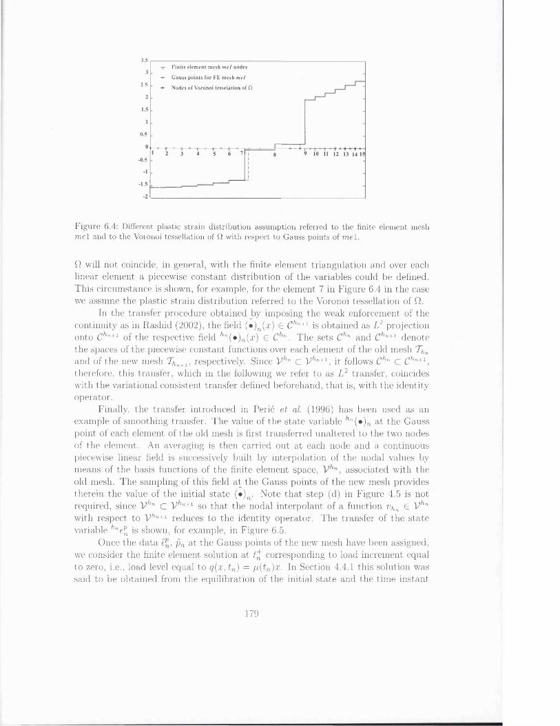
3.5F in ite e le m e n t m esh m e l nodes

G a u ss p o in ts fo r F E m esh m e l

N odes o f V o rono i te s se la tio n o f Q2.5

0.5

-0 .5

-1.5

F igure 6.4: Different plastic strain distribution assumption referred to the finite element mesh m el and to the Voronoi tessellation of Q with respect to Gauss points of m el.

Q will not coincide, in general, with the finite element triangulation and over each linear element, a piecewise constant distribution of the variables could be defined. This circumstance is shown, for example, for the element 7 in Figure 6.4 in the case we assume the plastic strain distribution referred to the Voronoi tessellation of Q.

In the transfer procedure obtained by imposing the weak enforcement of the continuity as in Rashid (2002), the field (*)n(:r) £ Chn+l is obtained as L2 projection onto Chn+1 of the respective field hn(»)n(x) E Chn. The sets Chn and Chn+1 denote the spaces of the piecewise constant functions over each element of the old mesh T^n and of the new mesh Thn+l, respectively. Since V hn C V/ln+1, it follows Chn C Chn+1, therefore, this transfer, which in the following we refer to as L 2 transfer, coincides with the variational consistent transfer defined beforehand, that is, with the identity operator.

Finally, the transfer introduced in Peric et al. (1996) has been used as an example of smoothing transfer. The value of the state variable hn(*)n at the Gauss point of each element of the old mesh is first transferred unaltered to the two nodes of the element. An averaging is then carried out at each node and a continuous piecewise linear field is successively built by interpolation of the nodal values by means of the basis functions of the finite element space, associated with the old mesh. The sampling of this field at the Gauss points of the new mesh provides therein the value of the initial state (*)n. Note that step (d) in Figure 4.5 is not required, since V hn C V/iri+1 so that the nodal interpolant of a function Vhn 6 V '1 with respect to Vhn+1 reduces to the identity operator. The transfer of the state variable /lne£ is shown, for example, in Figure 6.5.

Once the data pn at the Gauss points of the new mesh have been assigned, we consider the finite element solution at t* corresponding to load increment equal to zero, i.e., load level equal to q (x , tn) = fi(tn)x. In Section 4.4.1 this solution was said to be obtained from the equilibration of the initial state and the time instant

179

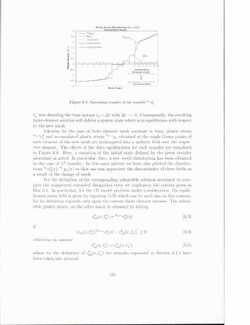
P la s tic S tr a in D i s t r i b u t io n s a t / u= 2 5 .5S m o o th in g 1 r a n s t e r

eSMsm ooth field

nodes old mesh

— i— nodes new mesh

e0.5

—a-

M c s h N o d e s

F igu re 6.5: Smoothing transfer of the variable ,ine£

t* was denoting the time instant tn + A t with A t —> 0. Consequently, the resulting finite element solution will deliver a system state which is in equilibrium with respect to the new mesh.

Likewise for the case of finite element mesh constant in time, plastic strain /'n+1ef1 and accumulated plastic strain hn+1pn obtained at the single Gauss points of each element of the new mesh are prolongated into a uniform field over the respec­tive element. The effects of the data equilibration for each transfer are visualized in Figure 6.6. Here, a variation of the initial state defined by the given transfer procedure is noted. In particular, then, a saw-teeth distribution has been obtained in the case of L2 transfer. In this same picture we have also plotted the distribu­tions hnepi{x), hnpn{x) so that one can appreciate the discontinuity of these fields asa result of the change of mesh.

For the definition of the corresponding admissible solution necessary to com­pute the augmented extended dissipation error we implement the criteria given in Box 6.1. In particular, for the ID model problem under consideration, the equili­brated stress field is given by equation (5.9) which can be used also in this context, for its definition depends only upon the current finite element stresses. The admis­sible plastic strain, on the other hand, is obtained by letting

£ , ( * ,£ ) = ( 6 - 3 )

ifaad{x,t+)[hn+1epn{x) - epad(x ,t~ )\ > 0, (6.4)

otherwise we assumeeadOMn) =eadOMn), (6.5)

where for the definition of epd(x, t~) the remarks expressed in Section 6.2.1 have been taken into account.

180

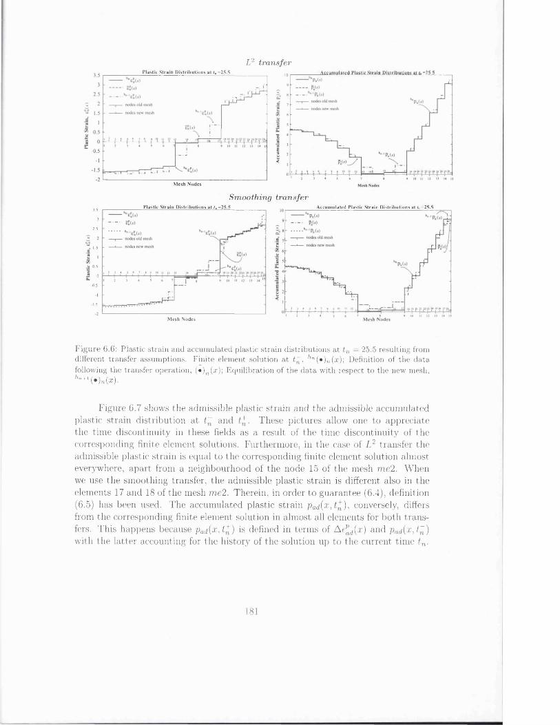
L2 tran sferP la s tic S t r a in D is t r ib u t io n s a t r „ = 2 5 .5

e

'SQm

-0 .5

M esh N odes

-A c c u m u la te d P la s tic S tra in P i$ t r ib u t iQns a t fa = 25 .5109

8

7

6

5

•v

33E3 2<

0

Sm ooth ing tra n sferP lastic S tra in D istrib u tio n s a t / ,= 25.5 A c c u m u la te d P la s tic S tr a in D is t r ib u t io n s a t r„= 25 .5

3.5

3

2.5

1.5c

W 0.5

0-0.5

1.5

M e s h N o d e s M esh Nodes

F igure 6.6: Plastic strain and accumulated plastic strain distributions at tn = 25.5 resulting from different transfer assumptions. Finite element solution a t t~, hn(»)n(x)-, Definition of the data following the transfer operation, (»)n (a:); Equilibration of the data with respect to the new mesh, ^ (•)»(*).

Figure 6.7 shows the admissible plastic strain and the admissible accumulated plastic strain distribution at t~ and t*. These pictures allow one to appreciate the time discontinuity in these fields as a result of the time discontinuity of the corresponding finite element solutions. Furthermore, in the case of L 2 transfer the admissible plastic strain is equal to the corresponding finite element solution almost, everywhere, apart, from a neighbourhood of the node 15 of the mesh m e2. When we use the smoothing transfer, the admissible plastic strain is different also in the elements 17 and 18 of the mesh m e2. Therein, in order to guarantee (6.4), definition (6.5) has been used. The accumulated plastic strain pad (x ,t+), conversely, differs from the corresponding finite element solution in almost all elements for both trans­fers. This happens because pad{x,t+) is defined in terms of Ae^d(x) and pad(x,t,~) with the latter accounting for the history of the solution up to the current time t n.

181

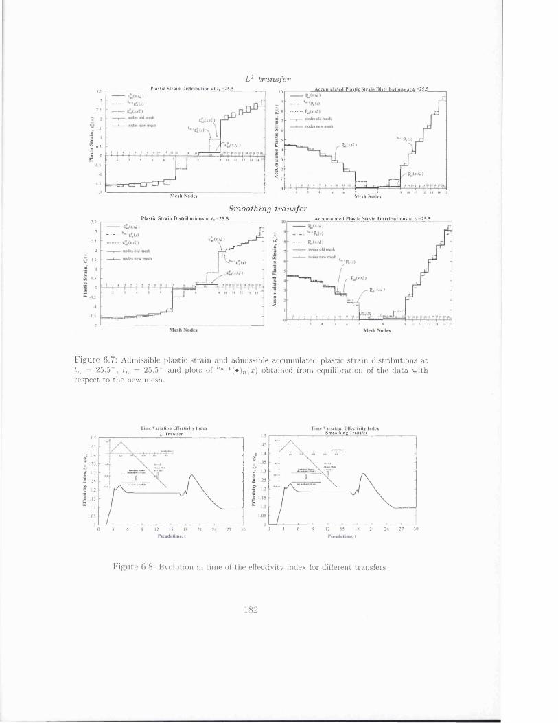
L 2 tran sferPlastic S tra in D istribu tion a t t n= 25.5

3.5

3

2.5

1.5

0.5

0-0.5

1.5

M esh Nodes

A ccum ulated P lastic S train D istribu tions at f,=25.5109

of

50.-o 4

33C3<I

0Mesh Nodes

Sm ooth ing tra n sferPlastic S tra in D istrib u tio n s a t t h= 25.5

3.5

3

2.5

21.5

0 5

0-0.5

1.5

-2

A ccum ulated P lastic S train D istribu tions a t fc=25.5

of=

2-•c3E3<

2 10 II 12 13 14 IS5

F igure 6.7: Admissible plastic strain and admissible accumulated plastic strain distributions at tn = 25.5~, tn = 25.5+ and plots of /,n+1 (•)n(x) obtained from equilibration of the data with respect to the new mesh.

rime V ariation EfTectivity Index L: T ran sfe r

T im e V ariation E ffcctiv itv Index

1.5

I 45

1.4

.35

1.3

.25

1.2

15

II1.05

I0 3 6 12 15 189 21 24 27 30

S m o o th in g T ra n sfe r

1.45

-oe

1=U

0 3 6 15 18 27 309 12 21 24

F igu re 6.8: Evolution in time of the effectivity index for different transfers

182

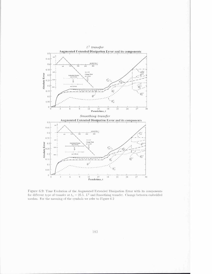
L2 tran sferA ugm ented E xtended D issipation E rror and its com ponents“i— --- 1------- 1------- 1------H------- 1-------- 1------- 1—1-----1--0.5

0.45

0.4

0.35

0.25

0.2

0.05

P seudotim e, t

S m ooth ing tra n sferA ugm ented E xtended D issipation Error and its com ponents

0.45

0.4

0.35

32 0.2•fl<

0.15

0.05

Pseudotim e, t

F igure 6.9: Time Evolution of the Augmented Extended Dissipation Error with its components for different type of transfer at tn = 25.5. L2 and Smoothing transfer. Change between embedded meshes. For the meaning of the symbols we refer to Figure 6.2

183

L2 tran sferS tress F ie ld s a t / n 25.5

A d m issib le an d c o n ju g a te to th e ad m issib le e la stic s tra in field

M esh N odes

Poin tw ise C o n tr ib u tio n to th e C u rre n t E r r o r in the E lastic L aw at =25 .5

W W W

(<*) (bSm ooth ing tra n sfer

Pointw ise C o n tr ib u tio n to the C u rre n t E r ro r in the E lastic Law a t =25.5M ress n e i a s a t t „ = Z5.5 A d m iss ib le a n d c o n ju g a te to th e ad m iss ib le e la s tic s t r a in field

(c) (ri)

F igure 6.10: The error in the elastic law at t = 25.5 + after change of mesh with different transfer assumptions (a) L2 transfer: Admissible stress oaci versus stress conjugate of the admissible elastic

strain Ce^d (b) L2 transfer: Pointwise contribution to the error in the elastic law, ^ ( ( 7ad — C e ^ )2

(c) Smoothing transfer: Admissible stress a(Ui versus stress conjugate of the admissible elastic strain

Ce^(l (d ) Smoothing transfer: Pointwise contribution to the error in the elastic law, — Ce®d)2

184

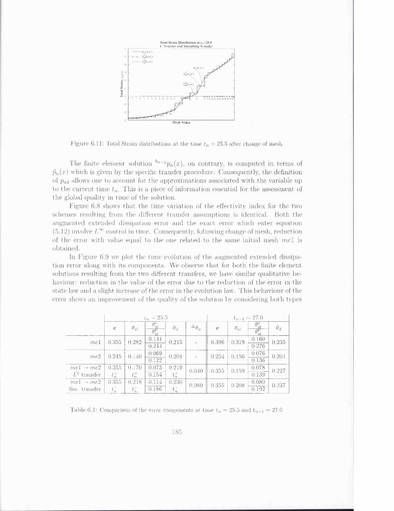
D T ransfer and Sm ooth ing Transfer65

e 2

£ 0

■I

-2

-3Mesh Nodes

F igure 6.11: Total Strain distributions a t the time tn = 25.5 after change of mesh

The finite element solution hn+1pn( x ), on contrary, is computed in terms of pn(x ) which is given by the specific transfer procedure. Consequently, the definition of pad allows one to account for the approximations associated with the variable up to the current time tn. This is a piece of information essential for the assessment of the global quality in time of the solution.

Figure 6.8 shows that the time variation of the effectivity index for the two schemes resulting from the different transfer assumptions is identical. Both the augmented extended dissipation error and the exact error which enter equation (5.12) involve L°° control in time. Consequently, following change of mesh, reduction of the error with value equal to the one related to the same initial mesh mel is obtained.

In Figure 6.9 we plot the time evolution of the augmented extended dissipa­tion error along with its components. We observe that for both the finite element solutions resulting from the two different transfers, we have similar qualitative be­haviour: reduction in the value of the error due to the reduction of the error in the state law and a slight, increase of the error in the evolution law. This behaviour of the error shows an improvement of the quality of the solution by considering both types

tn = 25. 5 71+1 = 27.0

0 i Pi ed A9,i Osl 0d

m el 0.355 0.282 0.141 0.215 0.396 0.319 0.160 0.2350.244 0.276

me 2 0.245 0.140 0.069 0.201 0.254 0.156 0.076 0.2010.122 0.136

m el —> me2 0.355 0.170 0.073 0.219 0.040 0.355 0.159 0.078 0.227L2 transfer t i Ln 0.154 t i 0.139

m el —> m e2 0.355 0.218 0.114 0.230 0.080 0.355 0.208 0.080 0.237Sm. transfer t i t i 0.186 t i 0.192

Table 6.1: Comparison of the error components at time tn = 25.5 and fn+i = 27.0

185

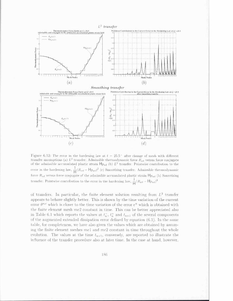
L2 t ran sferT h c rm o d v n a m ic F o rce F ields a t tn = 25.5

Adm issib le a n d c o n ju g a te fo th e ad m issib le accum ul ' ‘ _

R ^ (x .t i)

5' Hpjixji)

Poin tw ise C o n tr ib u tio n to the C u rre n t E r ro r in the H a rd e n in g Law a t =25.5In =u la ted p lastic s tra in Held

H i

M esh N odes

M esh Nodesir~

M esh Nodes

S m ooth ing tra n sfer

tUbul)

3.5 WpjLxJ i )

T h e rm o d y n a m ic F orce F ields a t tn = 25 .5 A dm issib le an d c o n ju g a te to the adm issib le a ccu m u la ted plastic s tra in field

Pointw ise C o n tr ib u tio n to the C u rre n t E r ro r in the H ard en in g Law at =25.5 04 ________________________ afte r Sm ooth ing tra n sfe r____________________

(c) (d)

F igure 6.12: The error in the hardening law at t = 25.5+ after change of mesh with different transfer assumptions (a) L 2 transfer: Admissible therm odynamic force Rad versus force conjugate of the admissible accumulated plastic strain (b) L2 transfer: Pointwise contribution to the

error in the hardening law, y^(Rad — H p af* )2 (c) Smoothing transfer: Admissible therm odynamic

force Rad versus force conjugate of the admissible accumulated plastic strain H p arf (b) Smoothing

transfer: Pointwise contribution to the error in the hardening law, t-t(Rad — Hpad)2H

of transfers. In particular, the finite element solution resulting from L 2 transfer appears to behave slightly better. This is shown by the time variation of the current error 9n,c which is closer to the time variation of the error en which is obtained with the finite element mesh m e2 constant in time. This can be better appreciated also in Table 6.1 which reports the values at t~, £+ and £n+1 of the several components of the augmented extended dissipation error defined by equation (6.1). In the same table, for completeness, we have also given the values which are obtained by assum­ing the finite element meshes m el and me2 constant in time throughout the whole evolution. The values at the time tn+1, conversely, are reported to illustrate the influence of the transfer procedure also at later time. In the case at hand, however,

186

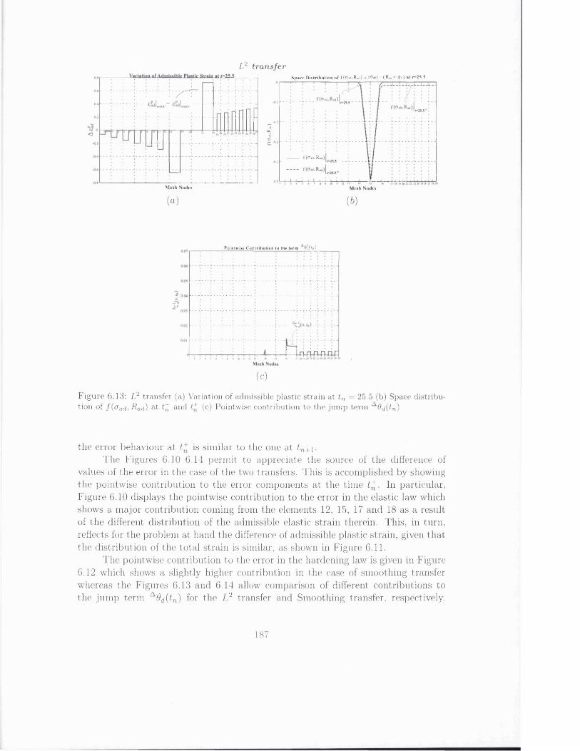
L2 tran sfer

(a)M esh N odes

S p a c e D is tr ib u tio n o f f(0*i,R »d) = I0 » jI - (R * i + cry) a t t= 25.5

-0.21cCi

5 --0 3

f (0*1, Rad)-0.4

-0.5

M esh N odes

(b)

Pointw ise C on trib u tio n to the te rm ©d(*u)

■ I In n n n n n

(c)

F igu re 6.13: L2 transfer (a) Variation of admissible plastic strain at tn = 25.5 (b) Space distribu­tion of f ( o ad, Rad) a t t~ and £+ (c) Pointwise contribution to the jum p term AOd{tn)

the error behaviour at t* is similar to the one at tn+\.The Figures 6.10-6.14 permit to appreciate the source of the difference of

values of the error in the case of the two transfers. This is accomplished by showing the pointwise contribution to the error components at the time £+. In particular, Figure 6.10 displays the pointwise contribution to the error in the elastic law which shows a major contribution coming from the elements 12, 15, 17 and 18 as a result of the different distribution of the admissible elastic strain therein. This, in turn, reflects for the problem at hand the difference of admissible plastic strain, given that the distribution of the total strain is similar, as shown in Figure 6.11.

The pointwise contribution to the error in the hardening law is given in Figure 6.12 which shows a slightly higher contribution in the case of smoothing transfer whereas the Figures 6.13 and 6.14 allow comparison of different contributions to the jump term A0d(t,n) for the L2 transfer and Smoothing transfer, respectively.

187

(a)

Variation of Admissible Plastic Strain at C=IS.

M esh N odes

Sm ooth ing tra n sferS p ace D is tr ib u tio n o f f(c r« i,R * d ) = la »JI - ( R*i + <3y) a t t= 25.5

1o'ic

M esh N odes

(b)Pointw ise C o n tr ib u tio n to the te rm 'O j(tn )

<

M esh Nodes

(c)

F igure 6.14: Smoothing transfer (a) Variation of admissible plastic strain at tn = 25.5 (b) Space distribution of f(crad> R a d ) at t~ and £+ (c) Pointwise contribution to the jum p term Add{tn)

For the latter case, the major contribution comes from the elements 14 and 15. In these elements, the smoothing transfer assumption produces a variation of admissible plastic strain, as shown in Figure 6.14(a), whereas the variation of f ( a ad, R ad), given in Figure 6.14(b) indicates that the behaviour associated with (crad, Rad) should be elastic, since / < 0 therein.

Finally, Figure 6.15 reports the classical measures of the error introduced in Section 6.2.1.2. These error measures exhibit the same qualitative behaviour as the augmented extended dissipation error with the reduction in the value of the error. They also show an improved behaviour of the finite element solution corresponding to the L 2 transfer. This is made clear from the time evolution of the current error of the generalised stress field ||ce ^ F ||, which is closer to the evolution of the global error II^gsfII■ The latter is obtained by assuming the constant finite element mesh m e2 throughout the whole loading process. Therefore, it can be said that the augmented extended dissipation error is capable to mirror the approximation associated with finite element solutions in the presence of change of mesh.

188

L2 tran sfer

* 4 ( 0 /

. -------- ‘< d(0 *4 ( 0 /........... * 4 (0

.................* K .(0 X

c« ”4 ( 0 «c.cd ( 0_

v 4 ( o y 'f

L C om p lem en ta ry Energy N orm of (he E xact E r ro r of the C S F co n juga te to the k inem atica lly adm issib le solution

0.35

1 03 >f 0.25

€ 02

* ~ § 015 ^ 0.1

005

— ecsf( o nc y' — - ‘* 4 ( 0 ' “ ( ' ) / ‘

...........* 4 ( 0 / . .> ..........

........... * 4 ( 0 X i

* c s f (0 / / j * g s f ( 0

^ / " ---------------1---------- — '

............................................................ e c « d ( o‘ .................. „ » r / \ *G.»(0

.......................................................... « W (0

S m ooth ing tra n sferC r N orm o f the E \a c t E r ro r o f the A dm issib le Total S train

(0 (0

(0 *"4(0Vkii(l)

LT C o m p lem en ta ry E nergy N orm o f the E xact E r ro r o f the G SF con ju g a te to the k inem atica lly adm issib le so lu tion

( 0

*gsf(0C°g sf ( 1 )

fk*V)^ ( 0

^ GSF ( 0

F igu re 6.15: Time Evolution of the Exact Error for different type of transfers at t n = 25.5. The meaning of the symbols used is the following: Vf € J , (•)(£) = sup ||(*)(x, r ) | |L2(n) and

T < t

c(*)(0 = ll(*)0M)||L2(n), whereas the superscripts ”o” , ”n, c” and ”n ” retain the usual meaning

189

Analysis of the error: Change betw een non—em bedded m eshesIn this second example, a change between non-embedded meshes is assumed to occur at the time tn = 25.5. As a result, the condition Vhn C Vhn+l is no more realized. Nevertheless, the mesh associated with Vhn+1 is chosen to contain a bigger number of elements. In particular, the new mesh me2es has been obtained by considering 28 linear equally spaced finite elements. Figure 6.16 shows the time discretization and the time instant when the change from the old mesh m el to the new mesh me2es occurs.

6.0 - -

pseudo-time, t

30.012.0 ' 18.0 24.06.0

-6 .0 - - At = 1.5 Change Mesh at t= 25.5Non-embedded Meshes

old mesh mel (14 els)

- 12.0 - -

new mesh me2es (28 els)

-18.0 - -

F igu re 6.16: Change between non-embedded meshes

Likewise the previous example, the three types of transfers introduced in Sec­tion 4.5 are next particularized for the change of mesh considered here.

When one adopts the variationally consistent transfer, the initial state e^(x), pn(x) is obtained by sampling the fields hne^(x) and hnpn(x) at the Gauss points of the new mesh, respectively. Consistently with the choice of one Gauss point per element for the integration of the constitutive equations, the fields hne^(x) and hnpn(x) are in turn assumed constant over each element of the old mesh. The piecewise value is equal to the computed finite element solution at the respective Gauss point of the element. Therefore, in order to determine the value of the data e ^ (x ) , pn(x) at the element Gauss point of the new mesh, x ^ p G f2gn+1, one needs to identify first the element f G T^n of the old mesh such that x ^q p G Then, by denoting with x fyp the Gauss point of the element Vt!}n, one assumes

( * ) n ( :Z:e ,G p ) “ / ln ( * ) n ( ^ G p ) (® -6)

If x^qp lies on the boundary of the element the average value of the variables between the two neighbouring elements is assumed. The definition of the variation­ally consistent transfer of the variable hne^(x) is visualized in Figure 6.17.

The initial state e^(x), pn(x) obtained from the weak enforcement of the con-

190

Pla stic S tra in D is tr ib u tio n s a t t„ = 2 5 .5Variationally consistent transfer

Gauss points

L

a.

Mesh Nodes

F igure 6.17: Variationally consistent transfer of /,ne^(x) for the definition of %( x )

Plastic Strain Distributions at /„=25.5 L ' transfer

---------- h"eH(x)

. .............— i— nodes old mesh

- ---- 1---- nodes new mesh

— x— Gauss points new mesh

a , ?

7 lr it ; f I( r j J1 2 1 4 5 A 10 II 12 13 14 13

Nue-Ctabrddnl Me.Sc.

_ ^ r J 0

■— —

Mesh Nodes

Figure 6.18: Weak enforcement of the continuity between the fields hne^(x) and e^(x)

tinuity with the fields hnepn(x), hnpn(x) as introduced in Rashid (2002) is given by

V e = 1 ,2 ,. . . , N hn+l

/l"(*)n(^)dx (6‘7)

( * ) n W = JXe'n+lhn+1 ~h--------x e - x^n

where N hn+1 is the number of elements in the triangulation T/ln+l and the superscript ”e” stands for element. The transfer defined by equation (6.7) assumes a constant value for (•)n(x) over each element fi£n+1. This value is equal to the weighted average of the field /ln(»)n(x), with the weight given by the area of the so called tributary regions. For the problem at hand, these regions are defined as the parts of the element, Q/eln+I — [x^n+1, x ^ 1], of the new mesh where the field hn(»)n(x) is constant. The definition of evn is visualized in Figure 6.18.

191

R em ark 6.1. Unlike the case V hn C V/ln+1, since now Vhn (£. V/in+1, the L2 transfer and the variat.ionally consistent transfer describe two different procedures which are not coincident with the identity operator. □

Finally, the smoothing transfer has been described in general in Figure 4.5. For the problem at hand, the transfer of the variable /luef1(.x') is given in Figure 6.19.

P lastic S tra in D is tr ib u tio n s a t fB=25.5

Gauss points ne\

c

M esh Nodes

F igure 6.19: Smoothing transfer of the variable hnepn(x)

The stresses obtained by solving the incremental constitutive equations with data e£, pn and the displacement field u^n - Uhn( x , t ~ ) are not in equilibrium with respect to the test functions associated with the new mesh. Therefore, the resulting residual must be equilibrated with consequent redistribution of the stresses and of the state variables. To achieve this, a finite element analysis with the new mesh and load increment equal to zero, i.e., load level equal to q(x, t n ) = p,(tn)x, is performed. In this manner, the ensuing finite element solution will deliver at t* a system state which is in equilibrium with respect to the new mesh.

The computed plastic strain /,n+1e£ and accumulated plastic strain hn+lp n ob­tained at the single Gauss points of each element of the new mesh are prolongated into a uniform field over the respective element. The effects of the data equilibra­tion for each transfer are visualized in Figure 6.20. In general, a variation of the initial state defined by the given transfer procedure is obtained. In particular, when the variationally consistent transfer is used, the initial state e^(x), p n(x) , by defini­tion, presents very little variation with respect to the finite element solution hneprl(x ) , l,np n ( x ) obtained on the old mesh mel. Consequently, the equilibration of the data with respect to the new mesh m e 2 e s produces a non uniform redistribution of plastic strain and accumulated plastic strain with concentration of plastic strain especially in the elements 23 and 27. This delivers a picture of the plastic strain distribution at t * which appears to be substantially different from he„(x) , where ht pn (x) denotes the plastic strain distribution at tn obtained from the finite element solution with mesh m e 2 e s constant throughout the whole evolution.

192

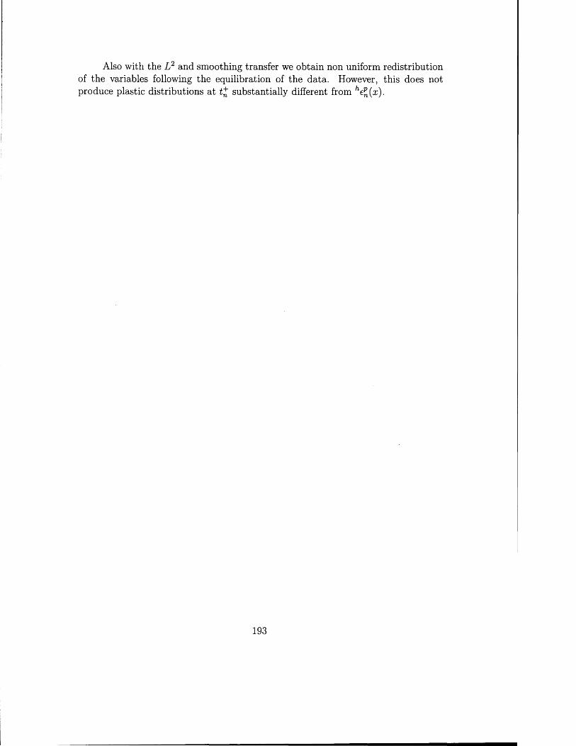
Also with the L 2 and smoothing transfer we obtain non uniform redistribution of the variables following the equilibration of the data. However, this does not produce plastic distributions at t+ substantially different from M M -

193

Plas

tic

Stra

in,

eH<

V aria tion a lly con s is ten t tran sfer

:"p„(x)IWtonodes old mesh nodes new mesh

nodes old mesh nodes new mesh

M esh Nodes M esh Nodes

L ’ tra n sferPlastic S train D istributions at t . =25.5

h"En(*)h*‘'6P„(x)hEP(x)nodes old mesh nodes new mesh

V'Pn(jr)Pn<*> nodes old mesh nodes new mesh

Mesh Nodes M esh Nodes

Sm ooth ing tra n sferPlastic Strain Distributions at l.= 2S.S

“Ejtr)nodes old mesh nodes new mesh

nodes old mesh nodes new mesh

Mesh NodesMesh Nodes

F igure 6.20: Plastic strain and accumulated plastic strain distribution at t n = 25.5 resulting from different transfer operations.

V aria tion a lly con s is ten t tran sferPlastic S tra in D istribution a t r„=25.5

£.

M esh Nodes

L2 tra n sferPlastic S train D istribution at r„= 25.5 Accum ulated Plastic S train D istributions at /,=25.5

c

-a

E<

2Mesh NoSes

10 II 12 13 14 IS

Sm ooth ing tra n sfe rPlastic S tra in D istribution al r. = 25.5

14 152-

2 10 II 12 13M esh Nodes Mesh Nodes

F igure 6.21: Admissible plastic strain and admissible accumulated plastic strain distribution at tn — 25.5“ , tn = 25.5+ and plots of /ln+1 (•)n(x) obtained from equilibration of the data with respect to the new mesh

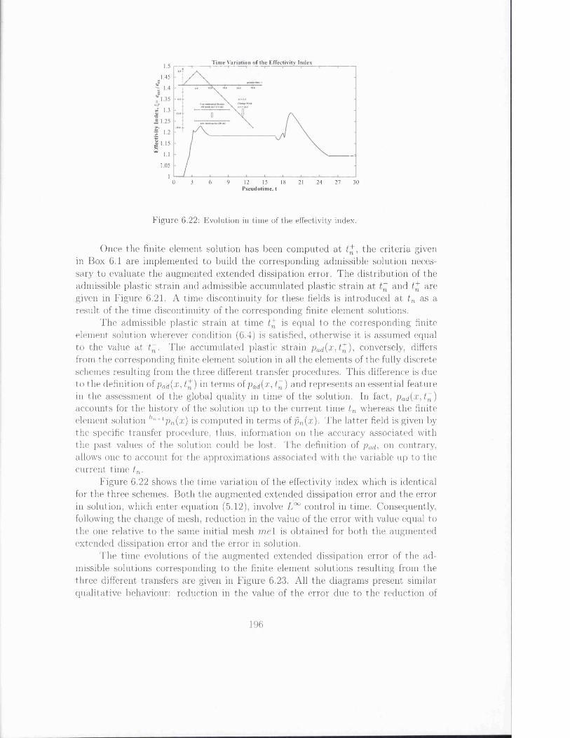
T im e V a r ia t io n o f th e E f f e c tiv ity In d e x

1 45

■as

>

1=u1.05

0 3 6 9 12 15 18 21 24 27 30P s e u d o t im e , t

F igure 6.22: Evolution in time of the effectivity index.

Once the finite element, solution has been computed at t+, the criteria given in Box 6.1 are implemented to build the corresponding admissible solution neces­sary to evaluate the augmented extended dissipation error. The distribution of the admissible plastic strain and admissible accumulated plastic strain at t~ and t* are given in Figure 6.21. A time discontinuity for these fields is introduced at t n as a result of the time discontinuity of the corresponding finite element solutions.

The admissible plastic strain at time t* is equal to the corresponding finite element solution wherever condition (6.4) is satisfied, otherwise it is assumed equal to the value at t~. The accumulated plastic strain p ad(x, £*), conversely, differs from the corresponding finite element solution in all the elements of the fully discrete schemes resulting from the three different transfer procedures. This difference is due to the definition of p„rf(x, t*) in terms of pad{x, t.~) and represents an essential feature in the assessment of the global quality in time of the solution. In fact, pact(x ,t~) accounts for the history of the solution up to the current time tn whereas the finite element solution lln+1pn{x) is computed in terms of pn{x). The latter field is given by the specific transfer procedure, thus, information on the accuracy associated with the past values of the solution could be lost. The definition of pad, on contrary, allows one to account for the approximations associated with the variable up to the current time t.n.

Figure 6.22 shows the time variation of the effectivity index which is identical for the three schemes. Both the augmented extended dissipation error and the error in solution, which enter equation (5.12), involve L°° control in time. Consequently, following the change of mesh, reduction in the value of the error with value equal to the one relative to the same initial mesh mel is obtained for both the augmented extended dissipation error and the error in solution.

The time evolutions of the augmented extended dissipation error of the ad­missible solutions corresponding to the finite element solutions resulting from the three different transfers are given in Figure 6.23. All the diagrams present similar qualitative behaviour: reduction in the value of the error due to the reduction of

196

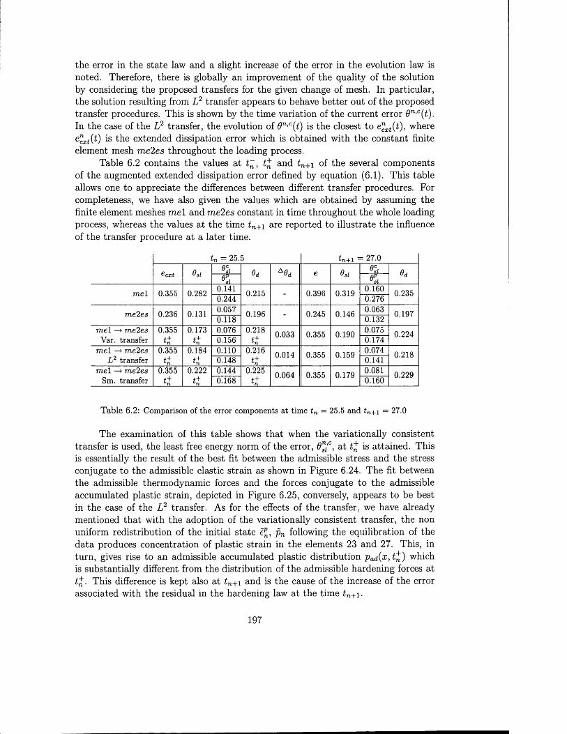
the error in the state law and a slight increase of the error in the evolution law is noted. Therefore, there is globally an improvement of the quality of the solution by considering the proposed transfers for the given change of mesh. In particular, the solution resulting from L2 transfer appears to behave better out of the proposed transfer procedures. This is shown by the time variation of the current error 6n,c(t). In the case of the L2 transfer, the evolution of 0n,c(t) is the closest to e xt(t), where egXf(£) is the extended dissipation error which is obtained with the constant finite element mesh me2es throughout the loading process.

Table 6.2 contains the values at t~, £+ and tn + 1 of the several components of the augmented extended dissipation error defined by equation (6.1). This table allows one to appreciate the differences between different transfer procedures. For completeness, we have also given the values which are obtained by assuming the finite element meshes m el and me2es constant in time throughout the whole loading process, whereas the values at the time tn + 1 are reported to illustrate the influence of the transfer procedure at a later time.

tn = 25.5 tn+l = 27.0

Cext 8 , 8j 8 , Vi 8dPsi

ua ua€

m el 0.355 0.282 0.141 0.215 0.396 0.319 0.160 0.2350.244 0.276

me2es 0.236 0.131 0.057 0.196 0.245 0.146 0.063 0.1970.118 0.132

me 1 —> me2es 0.355 0.173 0.076 0.218 0.033 0.355 0.190 0.075 0.224Var. transfer C 0.156 0.174

m el —> me2es 0.355 0.184 0 .1 1 0 0.216 0.014 0.355 0.159 0.074 0.218L 2 transfer 0.148 0.141

m el —► me2es 0.355 0 .2 2 2 0.144 0.225 0.064 0.355 0.179 0.081 0.229Sm. transfer 0.168 0.160

T able 6.2: Comparison of the error components at time tn = 25.5 and tn+1 = 27.0

The examination of this table shows that when the variationally consistent transfer is used, the least free energy norm of the error, 6™{°, at is attained. This is essentially the result of the best fit between the admissible stress and the stress conjugate to the admissible elastic strain as shown in Figure 6.24. The fit between the admissible thermodynamic forces and the forces conjugate to the admissible accumulated plastic strain, depicted in Figure 6.25, conversely, appears to be best in the case of the L2 transfer. As for the effects of the transfer, we have already mentioned that with the adoption of the variationally consistent transfer, the non uniform redistribution of the initial state e^, pn following the equilibration of the data produces concentration of plastic strain in the elements 23 and 27. This, in turn, gives rise to an admissible accumulated plastic distribution pad(^,t^) which is substantially different from the distribution of the admissible hardening forces at £+. This difference is kept also at tn+\ and is the cause of the increase of the error associated with the residual in the hardening law at the time £n+i-

197

W ith the L2 and smoothing transfer, on contrary, the error in the state law at tn + 1 decreases with respect to £+. This decrease can be considered due mainly to the enhanced approximation properties of the new interpolation space whose effects are soon evident on the variation of admissible plastic strain. Therefore, for these two transfers, unlike the variationally consistent transfer, the values of the error at t* can be assumed to reflect the effects more pertinent to the transfer procedure. For the variationally consistent transfer, on contrary, also the value of the error at tn + 1 must be considered.

Likewise the case of change between embedded meshes, Figures 6.26-6.28 al­low one to compare the different contributions to the jump term A9d(tn) for the transfer procedures under consideration. This appears to be highest in the case of the smoothing transfer assumption. The major contribution arises also here from the elements 15, 16 and 18 and must be related to the plastic strain which is therein introduced with the transfer and to the evolution of the admissible generalised stress field.

Finally, Figure 6.29 reports the classical measures of the error introduced in Section 6 .2.1.2. These diagrams present the same qualitative behaviour as the aug­mented extended dissipation error. Therefore, it is possible to assess the advantage of change of mesh which is to be related to the reduction in the value of the error. They also show a better behaviour of the admissible solution corresponding to the L2 transfer. This does appear from the time evolution of the current error of the generalised stress field \\ceQgF(t)\\. In fact, the variation of \\c€.gsf ( )\\ cl°ser t° the evolution of the global error ||e^5F(£)|| that is obtained by assuming the constant finite element mesh me2es throughout the loading process. Therefore, likewise the previous example, it can be said that the augmented extended dissipation error is capable to mirror the approximations associated with finite element solutions also in presence of change between non-embedded meshes.

198

V aria tion a lly con s is ten t tran sferA ugm ented E xten d ed D issipation E rror and its com p on en ts

0.35

<

0.05

0 3 6 9 12 15Pseudotim e, t

18 21 24 27 30

L2 tra n sferA u g m e n te d E x ten d ed D issip a tio n E rro r an d its co m p o n en ts

0.5

0.45

0.35

0.2

0.15

P se u d o tim e , t

Sm ooth ing tra n sferA u gm en ted E xten d ed D issip a tion E rror and its com p on en ts

i_ 0.3 ©

“ 0.25

<0.15

0 3 12 15P seudo tim e, t

6 9 18 21 27 3024

F igure 6.23: Time Evolution of the Augmented Extended Dissipation Error with its components for different type of transfer at tn = 25.5. Variationally consistent, L 2 and Smoothing transfer.

199

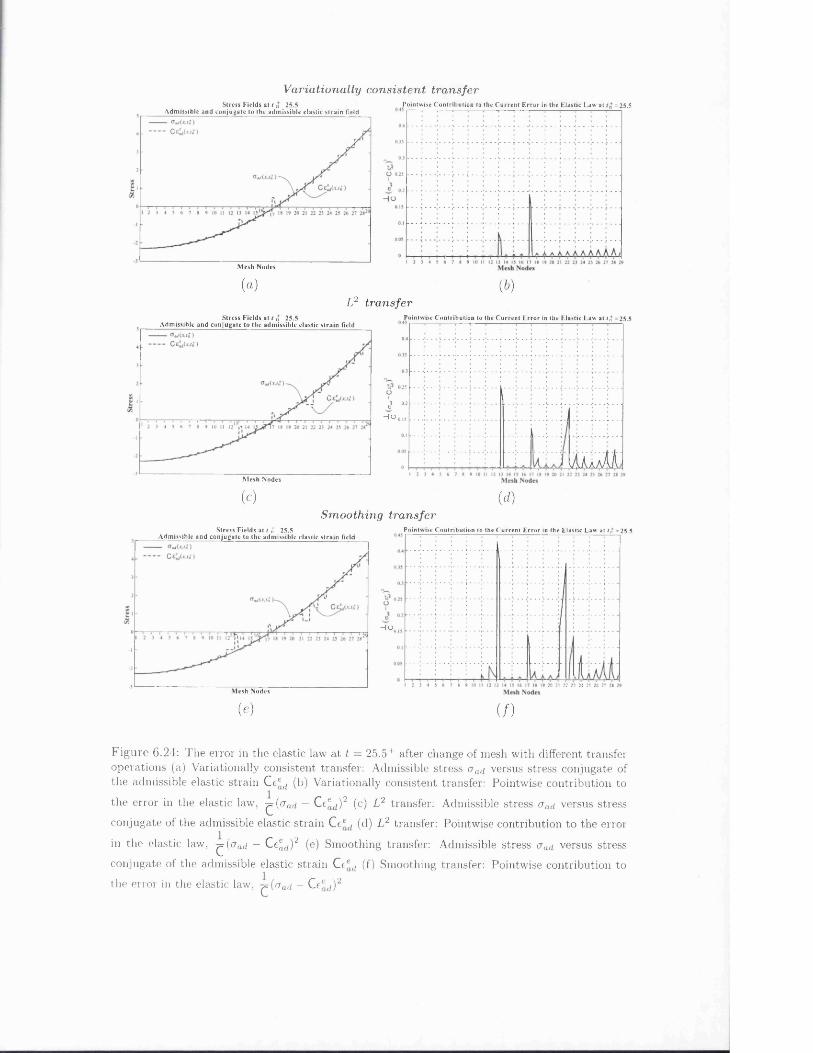
S tress F ie ld s a t t n 25.5 A d m issib le an d co n ju g a te to th e a d m iss ib le e la s tic s t r a in Held

M esh N odes

Varia tion a lly con s is ten t tran sferPoin tw ise C o n trib u tio n to the C u rre n t E r ro r in the E lastic Law a t =25.5

I 1

J...L.:

(a) (b)

S tre ss F ie ld s a t t n 25.5 A d m issib le a n d c o n ju g a te to th e a d m iss ib le e la s tic s t r a in field

M esh N odes

L2 tran sferPointw ise C o n tr ib u tio n to the C u rre n t E r ro r in the E lastic Law a t /„ =25.5

1 02 CH ° * I !

AlaAL( c ) od)

S m ooth ing tran sferS tre ss F ie ld s a t t nf 25.5

A d m iss ib le a n d c o n ju g a te to th e ad m is s ib le c la s tic s t r a in fieldPoin tw ise C o n trib u tio n to the C u rre n t E r ro r in the E lastic Law at /p =25.5

- l o ,

M esh N odes

(e) (/)

F igu re 6.24: The error in the elastic law at t — 25.5+ after change of mesh with different transfer operations (a) Variationally consistent transfer: Admissible stress a ad. versus stress conjugate of the admissible elastic strain Ce®d (b) Variationally consistent transfer: Pointwise contribution to

the error in the elastic law, ^(cra — Ce®d )2 (c) L2 transfer: Admissible stress oad versus stress

conjugate of the admissible elastic strain Ce®d (d) L2 transfer: Pointwise contribution to the error

in the elastic law, ~ (craci — Q tead)2 (e) Smoothing transfer: Admissible stress oad versus stress

conjugate of the admissible elastic strain Ce®fi (f) Smoothing transfer: Pointwise contribution to

the error in the elastic law, -^(aad - Ce®d)2

H qjxjt)

V aria tion a lly con s is ten t tran sferT h erm o d y n am ic F orce F ields a t tn = 25.5 Poin tw ise C o n tr ib u tio n to the C u rre n t E r ro r in the H a rd e n in g Law at

Adm issih le and con ju g a te to* the adm issib le accu m u la ted p lastic s tra in field

L2 tran sferT h erm o d y n am ic Force F ields a t tn = 25.5

A dm issible and co n juga te to the adm issib le accu m u la ted plastic s tra in field

----

Pointw ise C o n tr ib u tio n to th e C u rre n t F .rro r in the H a rd en in g Law a t /,* =25.5

( c )Sm ooth ing

T h e rm o d y n am ic F orce Fields a t tn = 2 5 .5 A dm issib le and co n juga te to*the adm issib le accu m u la ted plastic s tra in field

R«U'i)3 5 ----------

(d)tran sfer

Pointw ise C o n tr ib u tio n to the C u rre n t E r ro r in the H a rd en in g Law at =25.5

(e)

F igure 6.25: The error in the hardening law at t = 25.5+ after change of mesh with different transfer operations (a) Variationally consistent transfer: Admissible thermodynamic force Ra(i versus force conjugate of the admissible accumulated plastic strain Hpot/ (b) Variationally consistent

transfer: Pointwise contribution to the error in the hardening law, y j (R ad ~ Hpad)2 (c) L2 transfer:HAdmissible therm odynamic force R ad versus force conjugate of the admissible accumulated plastic

strain Y\pad (d) L2 transfer: Pointwise contribution to the error in the hardening law, p (Rad —HHpad)2 (e) Smoothing transfer: Admissible thermodynamic force Rad versus force conjugate of the admissible accumulated plastic strain Hpad (f) Smoothing transfer: Pointwise contribution to the

error in the hardening law, p- (Rad — Hpad)2

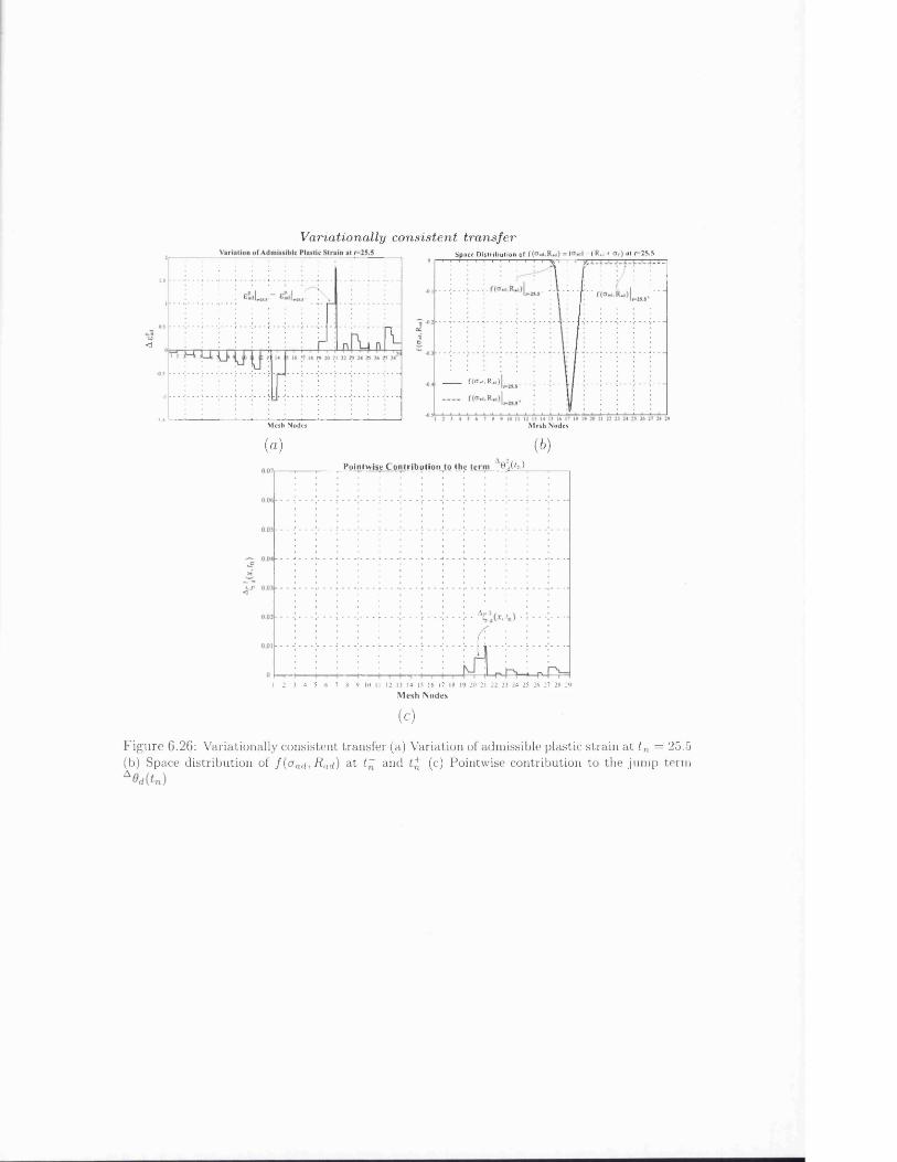
V aria tion a lly con s is ten t tran sfer

<

M esh Nodes

Space D istribu tion o f - ( R*j + a t f=25.5

f(ct«».R»d)

M esh Nodes

(a) (6)P o in tw is e C o n t r i b u t i o n to th e t e r m AB j( 'n )

A<s'

f‘ny '

— 1— — 1— — 1— — 1— — 1— I n r— p-1 2 3 4 5 6 7 8 9 10 II 12 13 14 15 16 17 18 19 20 21 22 23 24 25 26 27 28 29

M e s h N o d e s

(c)

F igu re 6.26: Variationally consistent transfer (a) Variation of admissible plastic strain at t n = 25.5 (b) Space distribution of / (<7ad, Rad) a t t~ and t f (c) Pointwise contribution to the jum p term

Ae

«

L 2 t ran sferV aria tion o f A dm issib le P lastic S tra in at t= 25.5

M esh Nodes

1CtLie>

(a)Pointw ise C on trib u tion to the term 0 d( ,n)

<

M esh N od es

(c)

F igu re 6.27: L2 transfer (a) Variation of admissible plastic strain at tn — 25.5 (b) Space distribu­tion of f ( a ad, Rad) at t~ and t~f (c) Pointwise contribution to the jum p term A9d{tn)

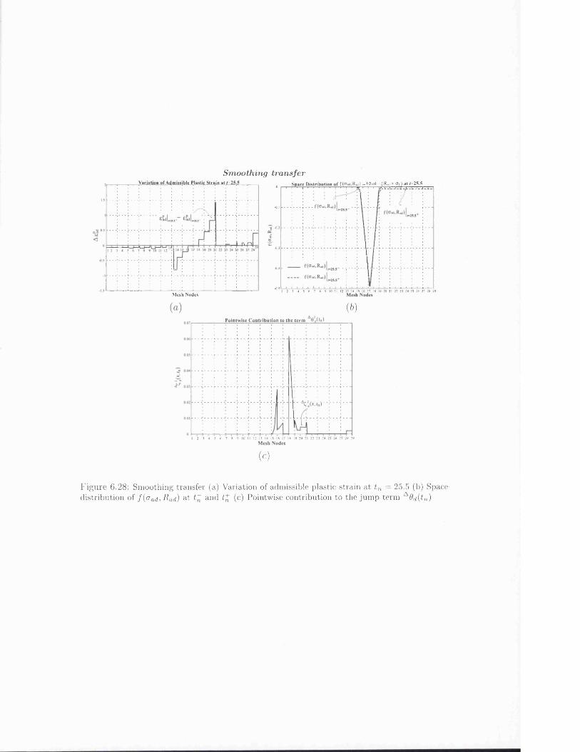
Sm ooth ing tran sferV aria tion of A dm issible Plastic S tra in at r=25

■API

M esh Nodes

S pace D istrib u tio n o f f R . » a ) = ia » i l - ( R ,d + a , ) a t f= 25.5 ! ' ! ■' ; ' ! '' ! ' ! ' f t ' ! 1 / - L - U J - a - L . U J - 4o

-0.1

-02

-0 3

-0.4

-0.58 9 10 II 12 13 14 15 16 1 18 IV 20 21 22 23 24 25 26 27 28 291 2 3 4 5 6

(6)P o in tw ise C o n tr ib u t io n to th e te rm

H<

24 25 26 27 2K 297 8 9 10 II 12 13 14 15 16 17 IK 19 20 21 22 232 3 4 5 6

(c)

F igu re 6.28: Smoothing transfer (a) Variation of admissible plastic strain at tn = 25.5 (b) Space distribution of f ( a ad, Rad) at t~ and t f (c) Pointwise contribution to the jum p term A0(i{tn)

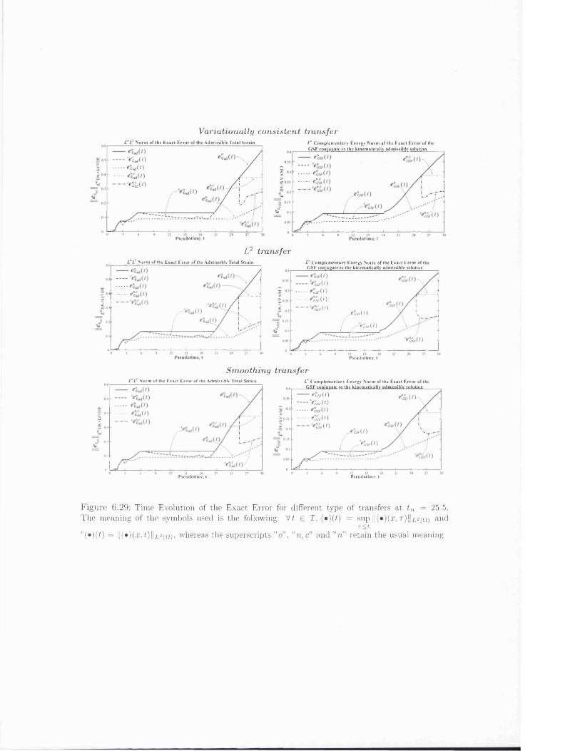
V aria tion a lly co n s is ten t tran sferL Lr N orm o f the E xact E r r o r o f th e A dm issib le T otal S tra in

e°E«i(0

Cad ( 0re'kL(l)

P seudotim e, t

T* C o m p lem en ta ry E nergy N orm o f the Exact E r r o r o f the G S F co n juga te to th e k inem atica lly adm issib le solution

P seudotim e, t

L2 tran sfer/-' / / N orm of the Exact E rro r o f the A dm issible Total S train C C o m plem en tary Energy Norm of the E xact E r ro r o f the

G SE con jugate to the k inem atically adm issible solution

g sf ( 1)

’c s f ( 0eGsr(‘)

Sf(')f c s A t )

*°c sfO )

Pseudotim e, t

S m ooth ing tran sferZ,*l ) N orm o f the Exact E r ro r o f the A dm issible Total S tra in

0.5

04

0.2

0213 6 12 15 IK

Pseudotim e, t24 27

> 0.25

S 0.2

C C o m plem en tary E nergy N orm o f the E xact E r ro r o f the GSF conjugate to the kinem atically adm issible solution____

e g s f ( t )

— C*°c;s f( O

• • • 0 e "asf( 0

ecsAh

‘ csA 0

e 'a sA I )

e'csf( 0

Pseudotim e, t

F igure 6.29: Time Evolution of the Exact Error for different type of transfers a t t n = 25.5. The meaning of the symbols used is the following: V£ £ X, (•)(£) = sup ||( • ) (a;,Tj||L2(n) an<J

T < t

c(«)(£) = ||(»)(x, £ ) ||l2(C2 )> whereas the superscripts ”o” , ”n, c” and ”n ” retain the usual meaning

6.3 Concluding remarksWhen the finite element mesh is changed at time instant tn, a discontinuity jump is introduced in the solution at the time instant tn. The jump produces a deterioration of the global accuracy of the approximation which is due both to the low order regularity of the approximation across the time node tn and to the eventual diffusion of inelastic deformations as a result of the transfer procedure. However, change of mesh along with suitable definition of the data can enhance the quality of the solution because of the improved approximation properties of the new finite element subspace. Therefore, the advantage of changing mesh with a transfer procedure depends on the interplay between the above opposing features.

In this chapter we have presented a general methodology for the assessment of the global quality of displacement finite element solutions of elastoplastic problems discretized in time with the backward Euler method on dynamically changing mesh.

This methodology employs the extended dissipation error, augmented by the term which accounts for the time discontinuity in the admissible solutions. The applicability of this new error estimator has been illustrated on a one dimensional model problem. Here, the behaviour of the finite element solution with respect to several definitions of transfer procedures and type of change of meshes has been considered. We have shown that the proposed error estimator reflects quite well the several sources of approximations, which result from the change of finite element mesh with the time step. Furthermore, the new error estimator accounts also for the improved approximation property, which arises from the enrichment of the finite element space and from suitable definition of the data on the new mesh. Therefore, the augmented extended dissipation error represents an effective tool for the critical assessment of the effects of transfer procedures for evolving meshes in small strain elastoplasticity.

206

Chapter 7

Conclusions

A general methodology for the assessment of the global quality of displacement finite element solutions of elastoplastic problems discretized in time with the backward Euler method on dynamically changing mesh has been presented.

The motivating idea has been the observation that change of data and/or finite element mesh from one time interval to the other can be both related to a discon­tinuity jump of the approximate solution across the time instant tn. Consequently, in the development of reliable a posteriori error estimates one needs to account not only for the time step and finite element mesh size but also for the value of the jump. Two simple error analysis of a first order ordinary differential equation, cho­sen as elementary prototype of the evolution law of the internal variables, show the influence on the error of the discontinuity jump, thus, the need for including such term in an a posteriori error estimate.

As a result, only measures of error that account for time discretization effects can reflect the low order regularity of the approximation across the time instant tn when the change of mesh occurs. Thus, the extended dissipation error introduced by Ladeveze et al. (1999) can be used for this aim. This is a measure of the error in the constitutive equations, that is, the state law and the evolution law, produced by an admissible solution which is time continuous, and satisfies the equilibrium and the kinematic conditions at any time instant.

The extended dissipation error capability to capture the effects of time and space discretization has been shown in the assessment of the quality of finite el­ement solutions of elastoplastic problems with the mesh constant throughout the loading process. Criteria to construct an admissible solution, which mirrors the approximations associated with the finite element solution, have been given for the Prandtl-Reuss plasticity model and illustrated with a numerical example. This has shown that all trends on the state law and dissipation contribution to the error were meaningful. Notable was also the comparison with classical measures of the exact error in solution showing that the extended dissipation error reflects quite well the evolution of the admissible solution with respect to the exact one as described by more classical measures of the error.

However, the extended dissipation error given in Ladeveze et al. (1999) assumes

207

time continuity of the admissible solution. Thus, in the second part of Chapter 3, we have defined a new measure of the error in the constitutive equations which accounts for the discontinuity jump in the admissible solution. The theory has been developed for rate-independent plasticity material models and exploits the observation that the solution of the initial boundary value problem, which governs the evolution of this class of material models, depends only on the sequence of load levels while time has just the function of ordering this sequence. Thus, fictitious continuous admissible processes have been defined over the time interval [tn, tn + At], with At not influential in the solution, along which the discontinuity was assumed to be taking place.

The analysis of the error in the constitutive equations along the aforementioned fictitious processes has lead to the definition of an additional nonnegative term which was depending on the jump, in agreement with the simple a posteriori error analysis of the first order differential equation. This term and the behaviour of the error component in the state law characterize completely the discontinuity jump. This is the content of Theorem 3.8 of Chapter 3 which motivates the use of the augmented extended dissipation error as basis of a methodology for the assessment of the global accuracy in time of finite element solutions on evolving meshes.

Applications of the theory have been presented for the displacement finite ele­ment solution of the Prandtl-Reuss plasticity model solved with incremental proce­dure. For this material model we have given the criteria to build admissible solutions as close as possible to the computed finite element solution.

The applicability of the methodology has been finally illustrated on a one di­mensional model problem where a detailed study of transfer operators (Ortiz &; Quigley, 1991; Peric et al., 1996; Rashid, 2002) has been carried out, with the nu­merical experiments providing confirmation of the theoretical developments. The augmented extended dissipation error was able to mirror the several sources of ap­proximations which are incurred by the change of finite element mesh with the time step. Also, it was able to account for the improved approximation property, which were arising from the enrichment of the finite element space and from suitable defi­nition of the data on the new mesh. Therefore, the augmented extended dissipation error has proven to be an effective tool for the critical assessment of the effects of transfer procedures for evolving meshes in small strain elastoplasticity.

7.1 Suggestions for further researchAlthough notable are the advances in the numerical simulation of more and more complex physical models, very little has been done on the corresponding side of assessment of the accuracy of the produced approximation.

This work has an aim to indicate a new way of designing adaptive strategies for problems solved with incremental procedure. In this sense, still further research is necessary. The following points bring up some issues that deserve special attention.

208

Definition of a new transfer.It has since been recognized that the issues of how to change mesh and the defini­tion of data is a very delicate matter in the adaptive solution of history dependent material models solved with incremental procedures.

To date, the available transfer operations have been introduced upon the re­quest to meet several vaguely defined properties which are invoked to prevent cor­rupting the quality of the resulting finite element solution (Ortiz k, Quigley, 1991; Peric et al., 1996; Rashid, 2002). With the methodology set in this work, a more rational treatment of the transfer operation seems possible to be devised in the con­text of the ensuing error. This should therefore lead to the definition of a transfer operation such as the one that minimizes the error produced. The definition of time step size, mesh size and indication on how to change mesh and to give data are not separate steps arising from heuristic arguments but should result from a unified analysis of the error contribution of each component.

E xtension to higher dim ensional problems.The theory presented in this work has been formulated in tensorial notations. Thus, its application to higher dimensional problems should not give further complica­tions apart from the implementation aspects. Criteria to build statically admissible stress fields are already in place (Ladeveze k Leguillon, 1983; Ladeveze et al., 1991; Ladeveze & Rougeot, 1997) whereas the definition of the other internal variables to build an admissible solution has been indicated in this work.

E xtension to viscoplasticity.The considerations of Section 3.5.2 cannot be carried over as they stand to a viscoplastic model. For example, in the viscoplastic model corresponding to the Prandtl-Reuss plasticity model (Ladeveze k Pelle, 2001), the dissipation potential <p(ep, — p) is given by

¥>(£” , - p ) = R o l l e l + ” + / c

where C is the same domain defined as in the Prandtl-Reuss plasticity model and

k , n are material constants, with n > 0. Thus, it follows that 7 =f > 1 . As an

result, in presence of a discontinuity jump in the internal variable p, p is a £-Dirac type distribution. Hence, (<5) 7 with 7 > 1 is no more a distribution (Schwartz, 1966) and the limit (3.49), which had been assumed as error associated with the discontinuity jump, is not finite.

In this case, it can be worth exploiting the following idea: Starting from the expression of the dissipation error for a time continuous fictitious admissible solution defined over [tn, tn + Tc], where Tc stands for a critical time to be computed, we assume that, for instance, the continuous admissible plastic strain has the following expression

ep(x ,t) = ep(x ,t~) + [ep{x,t+) - ep(x, t~)](p(t)

209

with the jump [ep]tn very small so that [€p]tn<p{t) may be assumed as a variation. Applying the methods of the calculus of the variations, we can state the following problem: For given Tc find the function (p(t) which minimizes the error.

The function <p(t) is required to meet the boundary conditions ip(t = 0) = 0, ip(t = Tc) = 1 and the minimization should be carried out in a-dimensional format so that a certain value for Tc can be computed.

The extension to viscoplasticity should also be such that when the viscoplastic model reduces to the corresponding rate independent model, the expression of the error reduces to the one obtained for the corresponding rate independent model.

210

Bibliography

A b b o , A . J . , & S l o a n , S. W . 1996. A n a u to m a tic lo ad s tep p in g a lg o rith m w ith e rro r con tro l. International Journal for Numerical Methods in Engineering, 39, 1737-1759.

A i n s w o r t h , M. 1996. The influence and selection of subspaces for a posteriori error estimators. Numerische Mathematik, 73, 399-418.

A i n s w o r t h , M., & O d e n , J. T . 1992. A procedure for a posteriori error esti­mation for h-p finite element methods. Computer Methods in Applied Mechanics and Engineering, 101, 73-96.

A i n s w o r t h , M., Sz O d e n , J. T . 1993. A unified approach to a posteriori error estimation using element residual methods. Numerische Mathematik, 65, 23-50.

A i n s w o r t h , M ., Sz O d e n , J . T . 1997. A p o ste rio ri e rro r e s tim a tio n in fin ite elem ent analysis. Computer Methods in Applied Mechanics and Engineering, 142, 1- 88 .

A i n s w o r t h , M., Sz O d e n , J. T. 2000. A Posteriori Error Estimation in Finite Element Analysis. John Wiley Sz Sons and B. G. Teubner.

A i n s w o r t h , M., Z h u , J. Z., C r a i g , A., Sz Z i e n k i e w i c z , O. C. 1989. Analysis ' of the Zienkiewicz-Zhu a posteriori error estimator in the finite element method. International Journal for Numerical Methods in Engineering, 28, 2161-2174.

A l b e r t y , J ., Sz C a r s t e n s e n , C. 2000. Numerical analysis of time-depending primal elastoplasticity with hardening. SIAM Journal on Numerical Analysis, 37, 1271-1294.

A l b e r t y , J., C a r s t e n s e n , C . , & Z a r r a b i , D. 1999. Adaptive numerical anal­ysis in primal elastoplasticity with hardening. Computer Methods in Applied Me­chanics and Engineering, 171, 175-204.

A l f a n o , G., R o s a t i , L., Sz VALORO SO, N. 1998. A displacement-like finite element model for J<i elastoplasticity: variational formulation and finite-step so­lution. Computer Methods in Applied Mechanics and Engineering, 155, 325-358.

211

A r m e r o , F . , Sz P e r e z - F o g u e t , A . 2002. O n th e fo rm u la tio n of c lo se s t-p o in t p ro jec tio n a lg o rith m s in e la s to p la s tic ity -p a r t I: T h e v a ria tio n a l s tru c tu re . Inter­national Journal for Numerical Methods in Engineering, 53, 297-329.

B a b u s k a , I . , &; M i l l e r , A . 1987. A feedback fin ite e lem ent m e th o d w ith a p o s te ­rio ri e rro r e s tim a tio n : P a r t I. T h e fin ite e lem ent m e th o d an d som e basic p ro p e rtie s of th e a p o s te rio ri e rro r e s tim a to r. Computer Methods in Applied Mechanics and Engineering, 61, 1-40.

B a b u s k a , I ., Sz R h e i n b o l d t , W . C . 1978a. E rro r e s tim a te s for ad ap tiv e fin ite e lem ent co m p u ta tio n s . SIAM Journal on Numerical Analysis, 15, 736-754.

B a b u s k a , I . , Sz R h e i n b o l d t , W . C . 1978b. A p o ste rio ri e rro r e s tim a te s for th e fin ite e lem ent m e th o d . International Journal for Numerical Methods in Engineer­ing, 1 2 , 1597-1615.

B a b u s k a , I . , Sz R h e i n b o l d t , W . C . 1979a. A nalysis o f o p tim a l f in ite -e lem en t m eshes in R 1. Mathematics of Computation, 33, 435-463 .

B a b u s k a , I . , Sz R h e i n b o l d t , W . C . 1979b. O n th e re liab ility a n d o p tim a lity of th e fin ite e lem ent m e th o d . Computers & Structures, 10, 87-94 .

B a b u s k a , I . , Sz R h e i n b o l d t , W . C . 1981. A p o ste rio ri e rro r analysis o f fin ite e lem ent so lu tio n s for o n e-d im en sio n a l p rob lem s. SIAM Journal on Numerical Analysis, 18, 565-589.

B a b u s k a , I . , Sz R o d r i g u e z , R . 1993. T h e p rob lem of th e se lection of a n a p o s te rio ri e rro r in d ica to r based on sm o o th en in g techn iques. International Journal for Numerical Methods in Engineering, 36, 539-567.

B a b u s k a , I . , Sz S t r o u b o u l i s , T . 2001. The Finite Element Method and its Reliability. O xford U niversity Press.

B a b u s k a , I . , Sz Y u , D . 1987. A sy m p to tica lly ex ac t a p o s te rio ri e rro r e s tim a to r for b iq u a d ra tic elem ents. Finite Elements in Analysis and Design, 3, 341-354.

B a b u s k a , I . , S t r o u b o u l i s , T . , Sz U p a d h y a y , C . S . 1994a. A m odel s tu d y of th e q u a lity of a p o s te rio ri e rro r e s tim a to rs for linear e llip tic p rob lem s. E rro r e s tim a tio n in th e in te rio r o f pa tchw ise un ifo rm grids of tr iang les. Computer Methods in Applied Mechanics and Engineering, 114, 307-378 .

B a b u s k a , I . , S t r o u b o u l i s , T . , U p a d h y a y , C . S ., G a n g a r a j , S. K ., Sz COPPS, K . 1994b. V alid a tio n of a p o s te rio ri e rro r e s tim a to rs by num erica l ap ­p roach . International Journal for Numerical Methods in Engineering, 37, 1073- 1123.

B a n k , R. E ., Sz S m ith , R. K . 1993. A p o ste rio ri e rro r e s tim a te s b ased on h ie ra rch ica l bases. SIAM Journal on Numerical Analysis, 30, 921-935.

212

B a n k , R . E . , & W e i s e r , A . 1985. Som e a p o s te rio ri e rro r e s tim a to rs for e llip tic p a r t ia l d ifferen tia l e q u a tio n s . Mathematics of Computation, 44, 283-301.

B a r l o w , J. 1976. Optimal stress locations in finite element models. International Journal for Numerical Methods in Engineering, 1 0 , 243-251.

B a r t h o l d , F . - J . , S c h m i d t , M ., Sz S t e i n , E . 1996. E rro r e s tim a tio n an d m esh a d a p tiv ity for e la s to -p la s tic d e fo rm ations. Z. Angew. Math. Mech.: Proceedings ICIAM/GAMM , 76, 159-162.

B a r t h o l d , F. J ., S c h m i d t , M., Sz S t e i n , E. 1997. Error estimation mesh adaptivity for elasto-plastic deformations. Pages 597-602 of: O w e n , D. R. J ., n a t e , E. O Sz H i n t o n , E. (eds), Computational Plasticity: Fundamentals and Applications. CIMNE.

B a r t h o l d , F .-J ., S c h m i d t , M., Sz S t e i n , E. 1998. Error indicators and mesh refinements for finite-element-computations of elastoplastic deformations. Com­putational Mechanics, 2 2 , 225-238.

B a t a i l l e , J., Sz K e s t i n , J. 1979. Irreversible processes and physical interpretation of rational thermodynamics. Journal of Non-equilibrium Thermodynamics, 4, 229-258.

B a t h e , K. J. 1996. Finite Element Procedures. Prentice-Hall.

B e r n a r d i , C ., Sz G i r a u l t , Y . 1998. A local reg u la riza tio n o p e ra to r for tr ia n g u la r a n d q u a d rila te ra l fin ite elem ents. SIAM Journal on Numerical Analysis, 3 5 , 1893- 1916.

B e s s o n , J ., C a i l l e t a u d , G., C h a b o c h e , J. L., Sz F o r e s t , S. 2001. Mecanique Non Lineaire des Materiaux. Hermes Science Publications.

B o n e t , J . , Sz W o o d , R . 1997. Nonlinear Continuum Mechanics for Finite Ele­ment Analysis. Cambridge University Press.

B o n e t , J., H u e r t a , A., Sz P e r a i r e , J. 2002. The efficient computation of bounds for functionals of finite element solutions in large elasticity. Computer Methods in Applied Mechanics and Engineering (in press).

B o r o o m a n d , B., Sz Z ie n k ie w ic z , O. C. 1998. Recovery procedures in error estimation and adaptivity. Adaptivity in non-linear problems of elasto-plasticity behaviour. Pages 383-410 of: L a d e v e z e , P ., Sz O d e n , J. T. (eds), Advances in Adaptive Computational Methods in Mechanics. Elsevier Science Ltd.

B r e n a n , K .E., C a m p b e l l , S.L., Sz P e t z o l d , L.R. 1996. Numerical Solution of Initial-Value Problems in Differential-Algebraic Equations. SIAM, Society for Industrial and Applied Mathematics.

213

B r e z i s , H. 1986. Analisi Funzionale: teoria e applicazioni. Liguori Editore. (In Italian).

B u s s y , P ., Sz R e m o n d , Y. 1985. D u a l i t e e n m e c a n iq u e d e s m a te r i a u x e t d e s

s t r u c u tu r e s . Internal Report 52. LMT-E.N.S. de Cachan, France. Lecture’s notes from the course by P. Ladeveze.

C a m a c h o , G . T . , Sz O r t i z , M . 1997. Adaptive Lagrangian modelling of ballistic penetration of metallic targets. Computer Methods in Applied Mechanics and Engineering, 142, 269-301.

C a r s t e n s e n , C., Sz F u n k e n , S. A. 2000. Averaging technique for FE-a posteriori error control in elasticity. Part I: Conforming FEM. Tech. rept. Mathematisches Seminar, Christian-Albrechts-Universitat zu Kiel, Germany.

C a r s t e n s e n , C., Sz V e r f u r t h , R. 1999. Edge residuals dominate a-posteriori error estimates for low order finite element methods. SIAM Journal on Numerical Analysis, 36, 1571-1587.

C h a b o c h e , J.L . 1996. Unified cyclic viscoplastic constitutive equations: Devel­opment, capabilities and thermodynamical framework. Pages 1-68 of: K r a u s z ,A .S ., Sz K r a u s z , K . (eds), Unified Constitutive Laws of Plastic Deformation. Academic Press.

C h e n , Z., N o c h e t t o , R. H., Sz S c h m id t , A. 2000a. A characteristic Galerkin method with adaptive error control for the continuous casting problem. Computer Methods in Applied Mechanics and Engineering, 189, 249-276.

C h e n , Z., N o c h e t t o , R. H., Sz S c h m id t , A. 2000b. Error control and adaptivity for a phase relaxation model. ESAIM-Mathematical Modelling and Numerical Analysis-Modelisation Mathematique et Analyse Numerique, 34, 775-797.

C i a r l e t , P. G. 1978. The Finite Element Method for Elliptic Problems. North Holland Publisher.

ClRAK, F . , Sz R a m m , E . 2000. A p o ste rio ri e rro r e s tim a tio n an d a d a p tiv ity for e la s to p la s tic ity using th e rec ip ro cal th eo rem . International Journal for Numerical Methods in Engineering, 47, 379-393.

C l e m e n t , P. 1975. Approximation by finite element functions using local regular­ization. Revue frangaise d ’automatique et de recherche operationnelle, 2 , 77-84.

C o f f i g n a l , G. 1987. Optimisation et Fiabilite des Calculs Elements Finis en Elastoplasticite. Ph.D. thesis, Universite Pierre et Marie Curie - Paris 6 , France.

C o l e m a n , B. D., Sz G u r t i n , M. E. 1967. Thermodynamics with internal state variables. The Journal of Chemical Physics, 47, 597-613.

214

C o m i , C., Sz P e r e g o , U. 1995. A unified approach for variationally consistent finite elements in elastoplasticity. Computer Methods in Applied Mechanics and Engineering, 121, 323-344 .

C o o r e v i t s , P ., D u m e a u , J .P ., Sz P e l l e , J. P . 1998. Error estimator and adaptivity for three-dimensional analysis. Pages 443~458 of: L a d e v e z e , P ., Sz O d e n , J. T. (eds), Advances in Adaptive Computational Methods in Mechanics. Elsevier Science Ltd.

C r i s f i e l d , M. 1991. Nonlinear Finite Element Analysis of Solids and Structures. Vol. 1. John Wiley Sz Sons, Inc.

D a w s o n , C., Sz K irb y , R. 1999. Solution of parabolic equations by backward Euler-mixed finite element, methods on a dynamically changing mesh. SIAM Journal on Numerical Analysis, 37, 423-442.

d e M i r a n d a , S., Sz U m b e r t i n i , F. 2002. Recovery of consistent stresses for com­patible finite elements. Computer Methods in Applied Mechanics and Engineering, 191, 1595-1609.

DE S a x c e , G. 1992. Une generalisation de l’inegalite de Fenchel et ses applications aux lois constitutives. Comptes Rendus Academie des Sciences, II, 314, 125-129.

d e S o u z a N e t o , E. A., P e r i c , D., Sz O w e n , D. R. J. 2002. Computational Plasticity: Small and Large Strain Finite Element Analysis of Elastic and Inelastic Solids. In Preparation.

D e m k o w i c z , L., D e v l o o , P h ., Sz O d e n , J. T. 1985. On h-type mesh- refinement strategy based on minimization of interpolation errors. ComputerMethods in Applied Mechanics and Engineering, 53, 67-89.

D e n n i s , J. E ., Sz S c h n a b e l , R. B. 1996. Numerical Methods for Unconstrained Optimization and Nonlinear Equations. SIAM, Society for Industrial and Applied Mathematics.

D i a z , A .R ., K i k u c h i , N., Sz T a y l o r , J .E . 1983. A method of grid optimiza­tion for finite element methods. Computer Methods in Applied Mechanics and Engineering, 41, 29-45.

D o r f l e r , W ., Sz W i l d e r o t t e r , O. 2000. An adaptive finite element method for a linear elliptic equation with variable coefficients. Z. Angew. Math. Mech., 80, 481-491 .

D r u c k e r , D . C . 1964. O n th e p o s tu la te of s ta b ili ty of m a te ria l in th e m echanics o f co n tin u a . Journal de Mecanique, 3, 235-249.

D u p o n t , T. 1982. Mesh modification for evolution equations. Mathematics ofComputation, 39, 85-107.

215

D u r a n , R., & R o d r i g u e z , R. 1992. On the asymptotic exacteness of Bank- Weiser’s estimator. Numerische Mathematik, 6 2 , 297-303.

D u v a u t , G., & L i o n s , J. L. 1976. Inequalities in Mechanics and Physics. Springer Verlag.

E k e l a n d , I., &; T e m a m , R. 1976. Convex Analysis and Variational Problems. North Holland Publisher.

E r i k s s o n , K., & J o h n s o n , C. 1991. Adaptive finite element methods for parabolic problems I: A linear model problem. SIAM Journal on Numerical Anal­ysis, 2 8 , 43-77 .

E r i k s s o n , K., E s t e p , D., H a n s b o , P ., & J o h n s o n , C. 1995. Introduction to adaptive methods for differential equations. Acta Numerica, 105-158.

E r i k s s o n , K., E s t e p , D., H a n s b o , P ., & J o h n s o n , C. 1996. Computational Differential Equation. Cambridge University Press.

E s t e p , D. J ., L a r s o n , M. G., & W i l l i a m s , R. D. 2000. Estimating the Error of Numerical Solutions of Systems of Reaction-Diffusion Equations. American Mathematical Society. Memoirs of the American Mathematical Society.

E v a n s , L. C. 1999. Partial Differential Equations. American Mathematical Society.

F l O R E N Z A , R. 1988. Elementi di Analisi Funzionale ed Applicazioni: Appunti delle Lezioni. Universita’ di Napoli-Italy. {In Italian).

F r a e i j s d e V e u b e k e , B. 1965. Displacement and equilibrium models in the finite element method. Chap. 9, pages 145-197 of: Z ie n k ie w ic z , O .C., &; H O L I S T E R ,

G.S. (eds), Stress Analysis. John Wiley &Sons.

F r e y , P. J ., & G e o r g e , P. L. 2000. Mesh Generation. Hermes Science Publica­tions.

F u c h s , M., & S e r e g i n , G. 2000. Variational Methods for Problems from Plasticity Theory and for Generalized Newtonian Fluids. Springer Verlag.

G a l l i m a r d , L. 1994. Contrdle adaptatif des calculs en elastoplasticite et en vis- coplasticite. Ph.D. thesis, LMT - E.N.S. de Cachan, France.

G a l l i m a r d , L ., L a d e v e z e , P ., & P e l l e , J .P . 1996. Error estimation and adaptivity in elastoplasticity. International Journal for Numerical Methods in Engineering, 3 9 , 189-217.

G a s t i n e , J . L ., L a d e v e z e , P . , M a r i n , P . , & P e l l e , J .P . 1992. A ccuracy an d o p tim a l m eshes in fin ite e lem ent c o m p u ta tio n for n early incom pressib le m a te ria ls . Computer Methods in Applied Mechanics and Engineering, 94 , 303-314.

216

G e a r , C.W . 1971. Numerical Initial Value Problems in Ordinary Differential Equa­tions. Prentice Hall.

G e r m a in , P, N g u y e n , Q. S., & S u q u e t , P. 1983. Continuum thermodynamics. Journal of Applied Mechanics - Transactions of the ASME, 50, 1010-1020.

G lo w i n s k i , R., L io n s , J. L., & T r e m o l i e r e s , R. 1981. Numerical Analysis of Variational Inequalities. North Holland Publisher.

G u r t i n , M. E. 1972. The Linear Theory of Elasticity. Pages 1-295 of: T r u e s d e l l , C., 8z F l u g g e (eds), Handbuch der Physik, vol. V Ia/2 . Springer Verlag.

G u r t i n , M .E. 1981. An Introduction to Continuum Mechanics. Academic Press.

H a l p h e n , B., &; N g u y e n , Q. S. 1975. Sur les materiaux standards generalises. Journal de Mecanique, 14, 39-63.

H a n , W ., & R e d d y , B. D. 1999. Plasticity: Mathematical Theory and Numerical Analysis. Springer Verlag..

H i l l , R. 1950. The Mathematical Theory of Plasticity. Oxford University Press.

H i n t o n , E., & C a m p b e l l , J. S. 1974. Local and global smoothing of discontin­uous finite element functions using a least square method. International Journal for Numerical Methods in Engineering, 8 , 461-480.

H i r i a r t - U r r u t y , J. B., &; L e m a r e c h a l , C. 2001. Fundamentals of Convex Analysis. Springer Verlag.

H j i a j , M. 1994. Sur la classe des materiaux standard implicites: Concept, Aspects discretises et Estimation de Terreur a posteriori. Ph.D. thesis, LMT - E.N.S. de Cachan, Prance.

H l a v a c e k , I. 1980. A fin ite e lem ent so lu tio n for p la s tic ity w ith s tra in hard en in g . Revue frangaise d ’automatique et de recherche operationnelle, 14, 347-368.

J o h n s o n , C. 1976a. Existence theorems for plasticity problems. Journal de Math- ematiques Pures et Appliquees, 55, 431-444.

J o h n s o n , C. 1976b. On finite element methods for plasticity problems. Numerische Mathematik, 26, 79-84.

J o h n s o n , C. 1977. A m ixed fin ite e lem ent m e th o d for p la s tic ity p rob lem s w ith hard en in g . SIAM Journal on Numerical Analysis, 14, 575-583 .

J o h n s o n , C. 1978. On plasticity with hardening. Journal of Mathematical Analysis and Applications, 62, 325-336.

217

J o h n s o n , C. 1994. A new paradigma for adaptive finite element method. Chap. 6 of: W h i t e m a n , J. R. (ed), The Mathematics of Finite Elements and Applica­tions. John Wiley &; Sons.

J o h n s o n , C., &; H a n s b o , P. 1992. Adaptive finite element methods in compu­tational mechanics. Computer Methods in Applied Mechanics and Engineering, 101, 143-181.

K a c u r , J. 1985. Method of Rothe in Evolution Equations. John Wiley & Sons andB. G. Teubner.

K e l l y , D.W . 1984. The self-equilibration of residuals and complementary a pos­teriori error estimates in the finite element method. International Journal for Numerical Methods in Engineering, 20, 1491-1506.

K r i e g , R .D ., &; K r i e g , D.B. 1977. A ccuracies of num erica l so lu tion m e th o d s for th e e la s t ic -pe rfec t ly plas tic m odel. Journal of Pressure Vessel Technology - Transactions of the ASME, 99, 510-515.

L a b o r d e , P ., & N g u y e n , Q. S. 1990. Etude de l’equation devolution des systemes dissipatifs standards. Modelisation Mathematique et Analyse Numerique, 24, 67-84.

L a d e v e z e , P. 1975. Comparaison de modeles de milieux continus. Ph.D. thesis, Universite Pierre et Marie Curie - Paris 6 , France.

L a d e v e z e , P. 1985. Sur une famille d’algorithmes en mecanique des structures. Comptes Rendus Academie des Sciences, //, 300, 41-44.

L a d e v e z e , P. 1989. La methode a grand increment de temps pour l’analyse des structures a comportement non lineaire decrit par variables internes. Comptes Rendus Academie des Sciences, II, 309, 1095-1099.

L a d e v e z e , P. 1994. La methode d ’ evaluation d ’ erreur en relation de comporte­ment appliquee a la MEF: qualite et amelioration. Internal Report 153. LMT- E.N.S. de Cachan, France.

L a d e v e z e , P. 1995. Les bases de la methode des erreurs en relation de comporte­ment pour le controle adaptatif des calculs elements finis: les travaux des annees 1977. Internal Report 163. LMT-E.N.S. de Cachan, France.

L a d e v e z e , P. 1999. Nonlinear Computational Structural Mechanics. Springer Verlag.

L a d e v e z e , P. 2001. Constitutive relation errors for F. E. analysis considering (visco-)plasticity and damage. International Journal for Numerical Methods in Engineering, 52, 527-542.

218

L a d e v e z e , P ., Sz L e g u i l l o n , D. 1983. Error estimate procedure in the finite element method and applications. SIAM Journal on Numerical Analysis, 2 0 , 485-509.

L a d e v e z e , P ., Sz M a u n d e r , E. A. W . 1996. A general method for recovering equilibrating element tractions. Computer Methods in Applied Mechanics and Engineering, 137, 111-151.

L a d e v e z e , P . , &; M o e s , N . 1997. A new a p o ste rio ri e rro r e s tim a tio n for n o n lin ea r tim e d ep en d en t fin ite e lem ent analysis. Computer Methods in Applied Mechanics and Engineering, 157, 45-68.

L a d e v e z e , P ., Sz M o e s , N. 1999. Adaptive control for finite element analysis in plasticity. Computers and Structures, 73, 45-60.

L a d e v e z e , P ., Sz O d e n , J. T. (eds). 1998. Advances in Adaptive Computational Methods in Mechanics. Elsevier Science Ltd.

L a d e v e z e , P ., Sz P e l l e , J .-P . 2001. La Maitrise du Calcul en Mecanique Lineaire et Non Lineaire. Hermes Science Publications.

L a d e v e z e , P ., & R o u g e e , P. 1984. Plasticite et viscoplasticite sous chargement cyclique. Internal Report 44. LMT-E.N.S. de Cachan, France.

L a d e v e z e , P ., Sz R o u g e o t , P h. 1997. New advances on a posteriori error on constitutive relation in f.e. analysis. Computer Methods in Applied Mechanics and Engineering, 150, 239-249.

L a d e v e z e , P . , C o f f i g n a l , G ., Sz P e l l e , J . P . 1986. Accuracy of elastoplastic and dynamic analysis. Chap. 11, pages 181-203 of: B a b u s k a , I . , Z ie n k ie w ic z , O . C ., G a g o , J., S z d e A. O l i v e i r a , E . R . (eds), Accuracy Estimates and Adaptive Refinements in Finite Element Computations. John Wiley & Sons.

L a d e v e z e , P ., P e l l e , J. P ., & R o u g e o t , P h . 1991. Error estimation and mesh optimization for classical finite elements. Engineering Computation, 8 , 69-80.

L a d e v e z e , P . , M o e s , N ., & D o u c h in , B . 1999. C o n s titu tiv e re la tio n e rro r e s tim a to rs for (v isco )p lastic fin ite e lem ent analysis w ith soften ing . Computer Methods in Applied Mechanics and Engineering, 176, 247-264.

L a r s s o n , F ., R u n e s s o n , K., Sz H a n s b o , P. 2001. Computation of goal-oriented a posteriori error measures in space-time finite elements for viscoplasticity. Pages 499-510 of: W a l l , W . A., B l e t z i n g e r , K. U., & S c h w e i z e r h o f , K. (eds), Trends in Computational Structural Mechanics. CIMNE.

L e T a l l e c , P. 1994. Numerical methods for nonlinear three-dimensional elasticity. Pages 465-622 of: C i a r l e t , P .G ., Sz L io n s , J.L (eds), Handbook of Numerical Analysis, vol. 3. Elsevier Science Ltd.

219

L e e , N., Sz B a t h e , K. J. 1994. Error indicators and adaptive remeshing in large deformation finite element analysis. Finite Elements in Analysis and Design, 16, 99-139.

L e m a i t r e , J ., Sz C h a b o c h e , J. L. 1990. Mechanics of Solid Materials. Cam­bridge University Press.

L u e n b e r g e r , D. G. 1984. Linear and Nonlinear Programming. Adison-Wesley Publishing Company, Reading, Mass.

M a l k u s , D. S., Sz H u g h e s , T. J. R. 1978. Mixed finite element methods - Reduced and selective integration techniques: a unification of concepts. Computer Methods in Applied Mechanics and Engineering, 15, 63-81.

M a u g i n , G. A. 1992. The Thermomechanics of Plasticity and Fracture. Cambridge University Press.

M i k h l i n , S. G. 1964. Variational Methods in Mathematical Physics. Pergamon Press.

M o e s , N. 1996. Une methode de mesure d ’erreur a posteriori pour les modeles de materiaux descrits par variables internes. Ph.D. thesis, LMT - E.N.S. de Cachan, France.

M o r e a u , J. J. 1974. On unilateral constraints, friction and plasticity. Pages 175- 322 of: C a p r i z , G., & S t a m p a c c h i a , G. (eds), New Variational Techniques in Mathematical Physics. Edizioni Cremonese.

N a d a i , A. 1937. Plastic behaviour of metals in the strain hardening range. Journal of Applied Physics, 8 , 205-213.

N g u y e n , Q. S. 1994. Bifurcation and stability in dissipative media (plasticity, friction, fracture. Applied Mechanics Review, 47, 1-31.

N g u y e n , Q. S. 2000. Stability and Nonlinear Solid Mechanics. John Wiley & Sons, LTD.

N o c h e t t o , R. H., S c h m i d t , A., Sz V e r d i , C. 1997. Adapting meshes and time steps for phase change problems. Atti Accademia Nazionale dei Lincei, 8 , 273-292.

N o c h e t t o , R. H., S a v a r e , G., Sz V e r d i , C. 2000. A posteriori error estimates for variable time step discretizations of nonlinear evolution equations. Communi­cations on Pure and Applied Mathematics, 53, 525-589.

O d e n , J. T ., D e m k o w i c z , L., R a c h o w i c z , W ., Sz W e s t e r m a n n , T. A. 1989. Toward a universal h-p adaptive finite element strategy. Part 2: A posteriori error estimation. Computer Methods in Applied Mechanics and Engineering, 77, 113— 180.

220

O r l a n d o , A., Sz P e r i c , D. 2000. A study on a posteriori error estimation for elastoplastic solids. In: Proceedings of the 6th International Conference on Com­putational Plasticity - COMP LAS VI.

O r t e g a , J. M., Sz R h e i n b o l d t , W . C. 2000. Iterative Solution of Nonlinear Equations in Several Variables. SIAM, Society for Industrial and Applied Math­ematics.

O r t i z , M ., Sz P o p o v , E . P . 1985. A ccuracy a n d s tab il i ty of in teg ra t io n a lgo r i thm s for e las top las t ic const i tu t iv e re la tions. International Journal for Numerical Meth­ods in Engineering, 21 , 1561-1576.

O r t i z , M ., & Q u i g l e y , J . J . 1991. A d ap tiv e m esh refinem ent in s tra in loca l­iza tio n prob lem s. Computer Methods in Applied Mechanics and Engineering, 9 0 , 781-804.

O r t i z , M ., Sz S t a i n i e r , L. 1999. The variational formulation of viscoplastic constitutive updates. Computer Methods in Applied Mechanics and Engineering, 1 7 1 , 419-444 .

P a n a g i o t o p o u l o s , P . D. 1985. Inequality Problems in Mechanics and Applica­tions. Birkhauser Boston Inc.

P a r a s c h i v o i u , M., P e r a i r e , J ., Sz P a t e r a , A. T. 1997. A posteriori finite ele­ment bounds for linear functional outputs of elliptic partial differential equations. Computer Methods in Applied Mechanics and Engineering, 1 5 0 , 289-312.

P a t e r a , A., Sz P e r a i r e , J. 2001. Implicit a posteriori computation of bounds. In: D e c o n i n c k , H., Sz B a r t h , T. J. (eds), VKI Lecture Series: Error Estimation and Solution Adaptive Discretization in CFD. Von Karman Institute, Belgium & NASA Ames Research Center, USA.

P e r i c , D., Yu, J ., Sz O w e n , D. R. J. 1994. On error estimates and adaptivity in elastoplastic solids: Applications to the numerical simulation of strain localization in classical and Cosserat continua. International Journal for Numerical Methods in Engineering, 37, 1351-1379.

P e r i c , D., H o c h a r d , C h . , D u t k o , M., Sz O w e n , D. R. J. 1996. Transfer operators for evolving meshes in small strain elasto-plasticity. Computer Methods in Applied Mechanics and Engineering, 1 3 7 , 331-344.

P r a g e r , W ., Sz S y n g e , J. L. 1947. Approximations in elasticity based on the concept of function space. Quarterly of Applied Mathematics, 5, 241-269.

R a d o v i t z k y , R., Sz O r t i z , M. 1999. Error estimation and adaptive meshing in strongly nonlinear dynamic problems. Computer Methods in Applied Mechanics and Engineering, 1 7 2 , 203-240.

221

R a n n a c h e r , R . , Sz S u t t m e i e r , F . T . 1997. A feed -back ap p roach to error contro l in finite e lem ent m ethods: app lica t ion to linear elasticity. Computational Mechanics, 19, 434-446.

R a n n a c h e r , R., Sz S u t t m e i e r , F. T. 1998. A posteriori error control in fi­nite element methods via duality techniques: Application to perfect plasticity. Computational Mechanics, 2 1 , 123-133.

R a n n a c h e r , R., Sz S u t t m e i e r , F. T. 1999. A posteriori error estimation and mesh adaptation for finite element models in elasto-plasticity. Computer Methods in Applied Mechanics and Engineering, 176, 333-361.

R a s h id , M . M . 2002. M ate ria l s ta te rem ap p in g in c o m p u ta tio n a l solid m echanics. International Journal for Numerical Methods in Engineering, 55, 431-450 .

R a v i a r t , P. A., Sz T h o m a s , J. M. 1977. Primal hybrid finite element methods for 2nd order elliptic equations. Mathematics of Computation, 31, 391-413.

R a v i a r t , P. A., Sz T h o m a s , J. M. 1983. Introduction a VAnalyse Numerique des Equations aux Derivees Partielles. Masson, Paris.

R e d d y , B. D ., Sz M a r t i n , J. B. 1994. Internal variable formulations of prob­lems in elastoplasticity: Constitutive and algorithmic aspects. Applied Mechanics Review, 47, 429-456.

R e i h e r , T h . 1987. An adaptive method for linear parabolic differential equations. Z. Angew. Math. Mech., 67, 557-565.

R e p i n , S. I., Sz X a n t h i s , L. 1996. A posteriori error estimation for elasto-plastic problems based on duality theory. Computer Methods in Applied Mechanics and Engineering, 138, 317-339.

RlSTlNMAA, M., Sz T r y d i n g , J. 1993. Exact integration of constitutive equations in elasto-plasticity. International Journal for Numerical Methods in Engineering, 36, 2525-2544.

ROCKAFELLAR, R. T. 1970. Convex Analysis. Princeton University Press.

R o d r i g u e z , R. 1994. Some remarks on Zienkiewicz-Zhu estimator. International Journal on Numerical Methods in Partial Differential Equations, 10, 625-635.

R o u g e o t , P. 1989. Sur le contrdle de la qualite des maillages elements finis. Ph.D. thesis, Universite Pierre et Marie Curie - Paris 6 , France.

S c h r e y e r , H.L., K u l a k , R .F ., Sz K r a m e r , J.M . 1979. Accurate numerical solutions for elastic- plastic models. Journal of Pressure Vessel Technology - Transactions of the ASME, 101, 226-234.

S c h w a r t z , L. 1966. Mathemathics for the Physical Sciences. Addison-Wesley.

222

S im o , J. C., Sz T a y l o r , R. 1985. Consistent tangent operators for rate independ- net elasto-plasticity. Computer Methods in Applied Mechanics and Engineering, 48, 101-118.

S im o , J. C., K e n n e d y , J. G., Sz T a y l o r , R. 1989. Complementary mixed finite element formulations for elastoplasticity. Computer Methods in Applied Mechanics and Engineering, 74, 177-206.

S im o , J.C . 1998. Numerical analysis and simulation of plasticity. Pages 183-499 of: C i a r l e t , P .G ., Sz L io n s , J .L (eds), Handbook of Numerical Analysis, vol. 6 . Elsevier Science Ltd.

S im o , J.C ., Sz H u g h e s , T .J .R . 1998. Computational Inelasticity. Springer Verlag.

S t e i n , E., Sz A h m a n d , R. 1977. An equilibrium method for stress calculation us­ing finite element displacements models. Computer Methods in Applied Mechanics and Engineering, 10, 175-198.

S t e w a r t , G. W. 1973. Introduction to Matrix Computations. Academic Press.

S t r o u b o u l i s , T ., S z H a q u e , K. A. 1992. Recent experiences with error estima­tion and adaptivity. Part I: Review of error estimators for scalar elliptic problems. Computer Methods in Applied Mechanics and Engineering, 97, 399-436.

S u l i , E., Sz HOUSTON, P. 2001. Adaptive finite element approximation of hy­perbolic problems. In: D e c o n i n c k , H ., Sz B a r t h , T. J. (eds), VKI Lecture Series: Error Estimation and Solution Adaptive Discretization in CFD. Von Kar- man Institute, Belgium Sz NASA Ames Research Center, USA.

SuQUET, P. 1981. Evolution problems for a class of dissipative materials. Quarterly of Applied Mathematics, 38, 391-414.

S y n g e , J.L . 1957. The Hypercircle in Mathematical Physics. Cambridge University Press.

T a b b a r a , M., B l a c k e r , T . , Sz B e l y t s c h k o , T . 1994. Finite element deriva­tive recovery by moving least square interpolants. Computer Methods in Applied Mechanics and Engineering, 117, 211-223.

Temam, R. 1985. Mathematical Problems in Plasticity. Gauthier-Villars.

T e m a m , R. 1986. A generalized Norton-Hoff model and the Prandtl-Reuss law of plasticity. Archive for Rational Mechanics and Analysis, 95, 137-183.

T e t a m b e , R. P ., Y u n u s , S. M., R a j a k u m a r , C., Sz S a i g a l , S. 1995. Exami­nation of flux projection-type error estimators in nonlinear finite element analysis. Computers & Structures, 54, 641-653.

223

T h o m e e , V. 1997. Galerkin-Finite Element Methods for Parabolic Problems. Springer Verlag.

V e r f u r t h , R. 1989. A posteriori error estimators for Stokes equations. Numerische Mathematik, 55, 309-325.

V e r f u r t h , R. 1996. A Review of A Posteriori Error Estimation and Adaptive Mesh-Refinement Techniques. Wiley-Teubner.

V e r f u r t h , R. 1999. A review of a posteriori error estimation techniques for elas­ticity problems. Computer Methods in Applied Mechanics and Engineering, 176, 419-440.

V i l l o n , P ., B o r o u c h a k i , H., Sz S a a n o u n i , K. 2000. Constrained interpolation based on plasticity criterion. In: Proceedings of the 6th International Conference on Computational Plasticity - COMP LAS VI.

W i b e r g , N. E ., Sz A b d u l w a h a b , F. 1993. Patch recovery based on superconver- gent derivatives and equilibrium. International Journal for Numerical Methods in Engineering, 36, 2703-2724.

W i b e r g , N. E., A b d u l w a h a b , F., & Z i u k a s , S. 1994. Enhanced superconver- gent patch recovery incorporating equilibrium and boundary conditions. Interna­tional Journal for Numerical Methods in Engineering, 37, 3417-3440.

Z h u , J . Z ., Sz Z i e n k i e w i c z , O. C. 1990. Superconvergent recovery technique and a posteriori error estimators. International Journal for Numerical Methods in Engineering, 30, 1321-1339.

Z i e n k i e w i c z , O. C., Sz T a y l o r , R. L. 2000. The Finite Element Method. Fifth edn. Vol. 1-3. Butterworth Heinemann.

Z i e n k i e w i c z , O. C., Sz Z h u , J. Z. 1987. A simple error estimator and adaptive procedure for practical engineering analysis. International Journal for Numerical Methods in Engineering, 24, 337-357.

Z i e n k i e w i c z , O. C., Sz Z h u , J. Z. 1992a. The superconvergent patch recovery and a posteriori error estimates. Part I: The recovery technique. International Journal for Numerical Methods in Engineering, 33, 1331-1364.

Z i e n k i e w i c z , O . C., Sz Z h u , J . Z. 1992b. The superconvergent patch recovery and a posteriori error estimates. Part II: Error estimates and adaptivity. International Journal for Numerical Methods in Engineering, 33, 1365-1382.

Z i e n k i e w i c z , O . C., Sz Z h u , J . Z. 1992c. The superconvergent patch recovery (SPR) and adaptive finite element refinement. Computer Methods in Applied Mechanics and Engineering, 101, 207-224.

224

Z i e n k i e w i c z , O. C., L iu , Y. C., & H u a n g , G. C. 1988. Error estimation and adaptivity in flow formulation for forming problems. International Journal for Numerical Methods in Engineering, 25, 23-42.

225