INTERNATIONAL JOURNAL FOR NUMERICAL METHODS IN ENGINEERING, VOL. 36, 837-854 (1993)

FINITE ELEMENT SIMULATION OF ADAPTIVE BONE REMODELLING: A STABILITY CRITERION

AND A TIME STEPPING METHOD

TIMOTHY P. HARRIGAN AND JAMES J. HAMI1.TON

School of Medicine, Department of Orthopedic Surgery, University of Missouri ut Kansas City Medicul School, 2301 Holmes S t . . Kunsas City, M O 64105, U.S.A.

SUMMARY

Adaptive bone remodelling simulations which use finite element analysis can potentially aid in the design of orthopedic implants and can provide examples which test specific bone remodelling hypotheses in a quantit- ative manner. By concentrating on remodelling algorithms in which the geometry is fixed but the tissue stiffness changes based on strain energy density, we have predicted stability conditions for bone remodelling and we have tested the applicability of thesc conditions using numerical simulations. The stability re- quirements arrived at using a finite element formulation are similar to the requirements arrived at in an earlier analytical study. In order to test the stability conditions, we have developed an Euler backward time stepping technique which uses the derivation for stability. These simulations arrived at solutions which were impossible using Euler forward time stepping as applied in this study. Cases in which a simplified version of the derived Euler backward method are unstable or marginally stable have also been seen, but when the Euler backward method is applied using the full derived matrices, no instabilities arc apparent. The results of the stability tests indicate that the converged density distributions in the examples studied are stable. Although u priori conditions which ensure stability are not found, a test for stability is provided, given an assumed density distribution.

INTRODUCTION

In the vertebrate skeleton, the influence of stress on tissue growth and maintenance is perhaps the most often cited example of mechanical effects in biology. Understanding this central process in animal growth and maintenance has been a focus of a great deal of research. This research has taken two general forms: the reductionist study of the microscopic mechanisms of bone formation in response to stress, and a more globally oriented simulation of bone remodelling, given some general rules for growth adapted from biological observations.

Although global study of bone remodelling through simulation is fundamentally unable to address the actual biologic events which form and resorb bone, an accurate simulation of bone remodelling is an important practical and theoretical tool. Such a simulation could identify prosthetic designs and design features which are likely to lead to problems due to stress shielding, and can show situations in which bone remodelling results in stresses within the prosthesis which could cause failure.3, 5 3 1 3 3 14, l 7 These simulations can also aid in the study of bone remodelling mechanisms, by indicating the mechanical relationships between bone stress and formation which result in a stable structure which accurately mimics actual bones.s366’7’10,11, l 7 Computerized simulations of bone remodelling thus potentially offer both a theoretical limit on the relationships

0029-5981/93/050837- 18$14.00 0 1993 by John Wiley & Sons, Ltd.

Received 13 Nouember 1991 Recised 4 M a y 1442

838 7. P. HARRIGAN AND 1. J. HAMILTON

between stress and bone response to it, and a practical tool for the design of bone repairs and total joint replacements.

In this paper, we use the term stability in the quantitative engineering sense. We are assessing whether we can guarantee that the size of any small perturbation around an equilibrium point will decay to zero with time. More precisely, we wish to guarantee that the eigenvalues of the linearized system equations all have negative real parts.

The process of bone remodelling uses an interrelationship between the microstructure of bone and global stiffness characteristics of the whole bone under load. The mechanism of bone remodelling is one where the stresses at a particular site in the bone cause bone tissue to be deposited or removed, yielding a change in the local stiffness of the bone or a change in the shape of the bone. The macroscopic shape and structure of the bones in the human skeleton are as variable as people themselves are, but they also share the degree of similarity that people share. Thus the microscopic processes which form and resorb bone yield a stable structure which adapt to the variable and common features which humans display.

In this study, we have used a finite element discretization to show an interrelationship between the bone remodelling process on a microscopic scale and the stability of the overall structure of bone on a global scale. We have also arrived at an effective method to simulate temporal changes in bone density distributions in response to stress.

The specific rule we have used for adaptation of bone to stress is one where the geometry of the bone remains constant, but the porosity of the tissue is changed in response to stress. With the algorithm used here, we intend to simulate the adaptation and maintenance of bone subjacent to synovial joints in the skeleton in the activities of daily living. Since we do not mimic changes in shape of the remodelling region in this study, growth and development are not studied here.

A scattered literature exists on mechanical effects in bone remodelling. The interdisciplinary nature of the subject contributes to this, as does the wide array of interested medical and scientific journals. Scientific studies on bone remodelling and on each of the many processes thought to be active in bone remodelling are found in journals as diverse as the processes studied. Mineraliz- ation, cell biology, collagen biochemistry, blood flow, mathematics, mechanics, and other topics of study can be applied to bone remodelling, and are. Thus a complete literature review is beyond the scope of this paper, and we will indicate primarily the literature which is relevant to our study.

The qualitative concepts put forth by W ~ l f f ~ ~ and the early anatomists have been recently explored using numerical models, but the original ideas are unsurpassed. Numerical modelling as applied to bone has primarily been aimed at simulating the bone remodelling concepts as proposed by the early anatomists. These studies are usually aimed at assessing whether the structure of bone can be predicted or developed using a particular mathematical remodelling rule. Considerable success has resulted from many of these studies; the density distribution of bone near joints, and the shape of long bone diaphyses can be predicted in a qualitative sense using the models developed so far. Thus these studies confirm the correctness of the original qualitative postulates made by the early anatomists.

Careful study of the particular artifices needed to arrive at realistic density distributions in these studies shows some theoretical problems, and offers an opportunity to go beyond the qualitative postulates of the early anatomists. The stability of the numerical bone remodelling simulations has been assessed in a number of recent studies. Carter el aL5 discussed convergence issues, as did Fhyrie and Hollister.8 Weinans et ~ 1 . ~ ~ 3 ~ ~ and Huiskes et d . 1 4 have explored the stability of bone remodelling simulations directly. Using a simplified model, Weinans et a1.23 indicated that the origin of the unstable behaviour was the remodelling rule, rather than the details of the finite element approximations. Huiskes et a1.I4 have shown that the density distribution in bone can be simulated, if the strain energy density from an intact bone is used as

FF SIMULATION OF ADAPTIVE BONE REMODELLING 839

the position-dependent ‘attractor state’ in a fairly coarse finite element mesh. The stability of this model was considered tenuous, and refinement of the finite element mesh was not attempted. Harrigan and Hamilton’ have indicated from an analytical model that the stability of bone remodelling simulations depends on the form of the remodelling rule. The analytical model resulted in the derivation of a stability limit for mechanical bone remodelling postulates, and showed that the unstable behaviour which rcsultcd from failure to satisfy the limit was not similar to the behaviour seen in viuo. The temporal stability of bone remodelling theories has been researched in terms of numerical experiments and analytical models, but analysis of the stability of finite element simulations per se has not been done in detail.

The results of a combined analytical and numerical investigation into the stability of bone remodelling simulations using finite element techniques are presented here. Since the Euler forward time stepping simulations used in this study developed instabilities which sccmed to be related to the Euler forward method as implemented here, an Euler backward method for time stepping the remodelling equations was developed. This method used the perturbation theory developed for the stability analysis. The method enabled the calculation of solutions which were impossible to obtain using the Euler forward method.

METHODS

The stability limit and the Euler backward time stepping method derived here are based on a particular hypothesis for bone remodelling, based on strain energy density. Other bone remodelling theories, based on stress and strain measures, have been developed. We chose to concentrate on a hypothesis based on strain energy density since it is mathematically simpler than stress measures, and since it has been shown to result in similar (but not identical) density distributions.’2 As will be seen below, taking the average strain energy density within a finite element is a very simple mathematical operation, especially within a finite element program. Thus in order to develop the mathematical detail necessary for physical insight into thc stability of finite element bone remodelling theories, we chose to use a strain-energy-density-based remodelling rule.

StuhiIity limit bused on finite element dtrrretization

An incremental analysis has been developed in order to study the reaction of the structure being investigated to small perturbations in density. For the purposes of the stability analysis, the structure being analysed is assumed to be at a state of remodelling equilibrium: i.e. we assume the density distribution has evolved to a steady state situation. Stability conditions in this analysis are developed using a standard method for study of a dynamic system, with the eventual tests for stability carried out using numerical methods.

In this development, and the development to follow regarding time stepping, the element matrices are written in global co-ordinates. The two indices are assumed to span the global range of global co-ordinate indices, with non-zero entries only in the positions in which the global co-ordinates couple to the ‘local’ co-ordinates of the element. Thus we never refer to local co-ordinates for the element stiffness matrices we use here. Also, the implied summation over repeated indices is used only when the repeated indices are subscripts which follow displacements or stiffness matrices. When summation over elements is implied, it is explicitly expressed using a summation sign. We also will use the subscripts f ; g, p and q to denote particular (global) degrees of freedom. The subscripts and left superscripts e and s refer to element number. When

840 T. P. HARRIGAN AND 1. J. HAMILTON

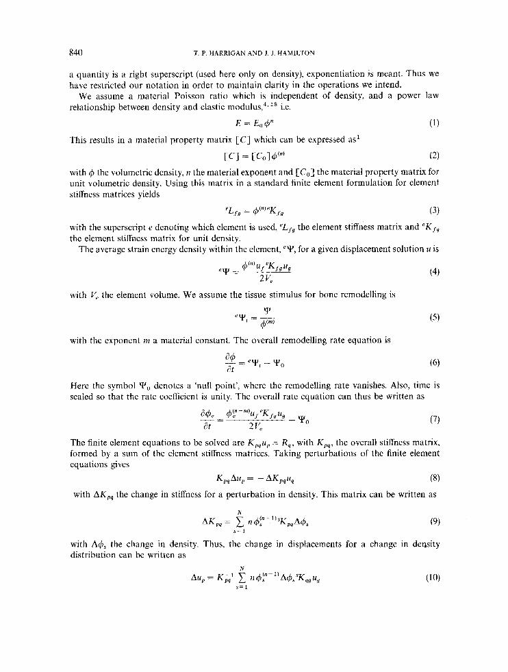
a quantity is a right superscript (used here only on density), exponentiation is meant. Thus we have restricted our notation in order to maintain clarity in the operations we intend.

We assume a material Poisson ratio which is independent of density, and a power law relationship between density and elastic m o d ~ l u s , ~ ~ i.e.

E = E,@’ (1)

CCl = CCOld‘”’ (2)

This results in a material property matrix [C] which can be expressed as1

with $ the volumetric density, n the material exponent and [C,] the material property matrix for unit volumetric density. Using this matrix in a standard finite element formulation for element stiffness matrices yields

eLfq = &‘“’eKfs (3)

with the superscript e denoting which element is used, ‘Lsg the element stiffness matrix and ‘ K f , the element stiffness matrix for unit density.

The average strain energy density within the element, “V, for a given displacement solution u is

with Ve the element volume. We assume the tissue stimulus for bone remodelling is

with the exponent m a material constant. The overall remodelling rate equation is

= Yt - ad, at

Here the symbol Y o denotes a ‘null point’, where the remodelling rate vanishes. Also, time is scaled so that the rate coefficient is unity. The overall rate equation can thus be written as

The finite element equations to be solved are K,,u, = R,, with KP4, the overall stiffness matrix, formed by a sum of the element stiffness matrices. Taking perturbations of the finite element equations gives

K,,Au, = - AK,,u, (8)

with AK,, the change in stiffness for a perturbation in density. This matrix can be written as

with distribution can be written as

the change in density. Thus, the change in displacements for a change in density

FE SIMULATION OF ADAPTIVE BONE REMODELLING 84 1

Perturbations in the rate equation, assuming a converged state, can be written as

~ S(Aq5,) (@-") + (n - m ) @ t m-1)Aq5,)(ufeKJ.gug + 2ufeKfsAu, + AufL'KrqAug) - y o -

at 2 v e

where we have used the fact that the element stiffness matrices are symmctric. Cancelling terms, neglecting higher order terms in perturbations, and substituting for AU gives

with

and

with ii,, equal to 1 if e = s, and zero otherwise. Based on a solution which is an exponential in time, the solutions of equation (9) will decay

with time, and the equilibrium state arrived at will be stable, i f the matrix M , , + D,, is negative definite. A matrix is negative definite if all thc cigcnvalues of the matrix have negative real parts. Since the matrix derived here is non-symmetric, the eigenvalues will be complex numbers, and special techniques for eigenvalue extraction are needed to compute them.

The stability of this matrix can be assessed, however, if two facts are used: (A) the matrix is stable if (and only if) the symmetric part of the matrix is stable;15 and (B) a symmetric matrix is positive definite if (and only if) the LDLT factorization of the matrix yields a diagonal matrix D in which all the diagonal coefficients are greater than zero.2o We use fact (A) by calculating only the symmetric part of the matrix M,, + Des; we use fact (B) by taking the negative of this matrix and doing LDLT factorization. Since the LDLT factorization of a symmetric matrix is available using a standard finite element equation solver,' investigating the stability of the matrix Me, + D,, can be conveniently done using the tools of standard finite element analysis.

Calculation of the coefficients in M e , would appear to be prohibitive, but since the LDLT factorization of the overall finite element stiffness matrix is already available after the finite clement solution for displacements ( K U = R), the cocfficicnts in M,, can he found as follows: calculate the element stiffness matrix [ K o l S , form the product [ K , ] , U , then use back substitu- tion to find [ K - ' ] [ K 0 ] , 9 U . A dot product between [Ko] ,U and [ K - ' ] [ K O ] , U will yield M,,. Thus, the finite element matrix does not need to be inverted to form Me,, but a large number of back substitutions must be performed. Practically, the element matrix dot products and the results of the back substitution [ K - ' I [ K , ] , U are calculated once for each element and stored on disk.

Time stepping algorithms for density changes due to stress

In order to simulate the adjustment of bone to the stresses placed on it, we have used two different time stepping algorithms, referred to as Euler forward' and Euler backward.' In both cases, we chose a uniform initial density distribution and time stepped equation (6) to arrive at a final density distribution. The test for stability was made if the time stepping algorithms were successful in obtaining a solution. As we have seen from other work,g the ability to arrive at

842 T. P. HARRIGAN AND J. J. HAMl1,TON

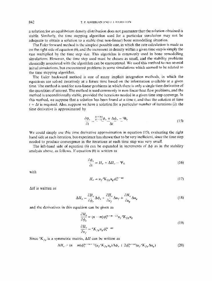
a solution for an equilibrium density distribution does not guarantee that the solution obtained is stable. Similarly, the time stepping algorithm used for a particular simulation may not be adequate to obtain a solution to a stable (but non-linear) bone remodelling situation.

The Euler forward method is the simplest possible one, in which the rate calculation is made as on the right side of equation (6), and the increment in density within a given time step is simply the rate multiplied by the time step size. This algorithm is commonly used in bone remodelling simulations. However, the time step used must be chosen as small, and the stability problems classically associated with the algorithm can be encountered. We used this method to run several initial simulations, but encountered problems in some simulations which seemed to be related to the time stepping algorithm.

Thc Euler backward method is one of many implicit integration methods, in which the equations are solved iteratively at a future time based on the information available at a given time. The method is used for non-linear problems in which there is only a single time derivative of the quantities of interest. The method is used commonly in non-linear heat flow problems, and the method is unconditionally stable. provided the iterations needed in a given time step converge. Tn this method, we suppose that a solution has been found at a time f , and that the solution at time t + At is required. Also, suppose we have a solution for a particular number of iterations (i): the time derivative is approximated by

We could simply use this time derivative approximation in equation (15). evaluating the right hand side at each iteration, but experience has shown that to be very inefficient, since the time step needed to produce convergence in the iterations at each time step was very small.

The left-hand side of equation (6) can be expanded in increments of A$ as in the stability analysis above. as follows. If equation (6) is writtcn as

with

AH is written as

and the derivatives in this equation can be given as

Since ' K f s is a symmetric matrix, AH can be written as

FE SIMULATION OF ADAPTIVE BONE REMODELLING 843

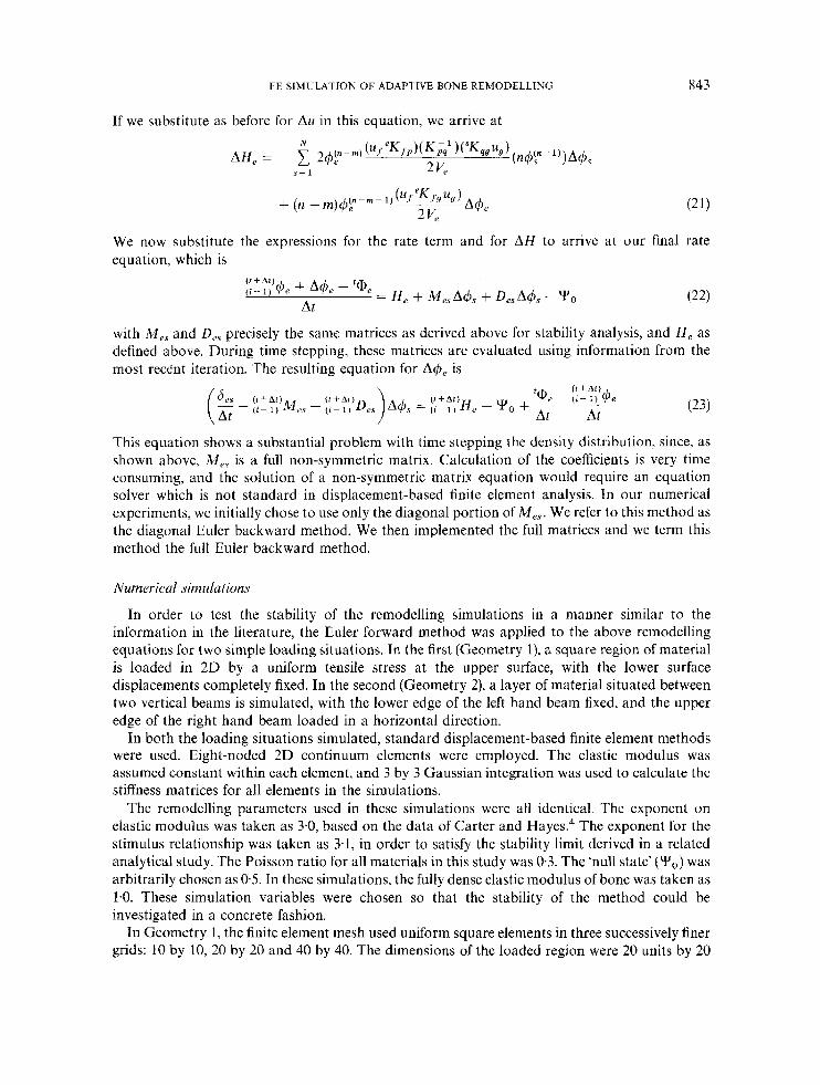
If we substitute as before for Au in this equation, we arrive at

We now substitute the expressions for the rate term and for equation, which is

(21)

AH to arrive at our final rate

with M , , and D,, precisely the same matrices as derived above for stability analysis, and H , as defined above. During time stepping, thcse matrices are evaluated using information from the most recent iteration. The resulting equation for A4, is

This equation shows a substantial problem with time stepping the density diftribution, since, as shown above, M,, is a full non-symmetric matrix. Calculation of the coefficients is very time consuming, and the solution of a non-symmetric matrix equation would require an equation solver which is not standard in displacement-based finite element analysis. In our numerical experiments, we initially chose to use only the diagonal portion of M e s , We refer to this method as the diagonal Euler backward method. We then implemented the full matrices and we term this method the full Euler backward method.

Numer lcal sim ulu t ions

In order to test the stability of the remodelling simulations in a manner similar to the information in the literature, the Euler forward method was applied to the above remodelling equations for two simple loading situations. In the first (Geometry l), a square region of material is loaded in 2D by a uniform tensile stress at the upper surface, with the lower surface displacements completely fixed. In the second (Geometry 2), a layer of material situated between two vertical beams is simulated, with the lower edge of the left hand beam fixed, and the upper edge of the right hand beam loaded in a horizontal direction.

In both the loading situations simulated, standard displacement-based tinite element methods were used. Eight-noded 2D continuum elements were employed. The elastic modulus was assumed constant within each element, and 3 by 3 Gaussian integration was used to calculate the stiffness matrices for all elements in the simulations.

The remodelling parametcrs used in these simulations were all identical. The exponent on elastic modulus was taken as 3.0, based on the data of Carter and Hayes.4 The exponent for the stimulus relationship was taken as 3.1, in order to satisfy the stability limit derived in a related analytical study. The Poisson ratio for all materials in this study was 0-3. The 'null state' (Yo) was arbitrarily chosen as 0.5. In these simulations, the fully dense elastic modulus of bone was taken as 1.0. These simulation variables were chosen so that thc stability of the method could be investigated in a concrete fashion.

In Geometry I, the finite element mesh used uniform square elements in three successively finer grids: 10 by 10,20 by 20 and 40 by 40. The dimensions of thc loaded region were 20 units by 20

844 T P HARRIGAN AND J. J. HAMILTON

units, and a net load of 0.6 force units was applied to thc top of the mesh. This test of the remodelling situation was motivated by the experiences of Weinans et a1.22,23 in which remodel- ling simulations (with n = 3, rn = 1) were found to be unstable for more refined finite element meshes.

In Geomctry 2, the material within the beams did not changc with time, but the stiffness of the material within the layer changed according to the remodelling rule discussed above. The remodelling region was I0 units wide and 100 units tall. Both beams were 5 units wide and 100 units tall. The lcngth of the beams and the remodelling area was spanned by 100 even elements. The remodelling region was 10 elements thick, and both beams were 5 elements thick. The net load on the right hand beam was 0.3 force units.

The initial volumetric density of the remodelling material was chosen as 0.5 for all cases, except for two cases in which the Euler forward method was used in Geometry 1. In these cases, the 10 by 10 and the 20 by 20 finite element simulations were given initial density distributions which were 0.5 in all but a few regions. In these regions, the initial density was moved upward to 0.8 or downward to 0.3 in order to assess the behaviour of perturbations in the initial density distribution as time went on.

Simulation scaling. Since the equations used in the simulations are fairly simple (equation ( 6 ) and KU = R in the finite element modcl), we can scale the simulation variables to solve a number of problems with the same simulation. If the actual finite element stiffness matrices (K), the actual load (k ) and the actual value of the null state (?o) are scaled from the values in the simulations by

I Z = a K , R = f i R , Yo=yYo

then the actual nodal point displacements are the simulation displacements multiplied by x i / . Inserting these scaling factors into equation (6) shows an interrelationship between the three scaling factors which is

-

By choosing the elastic modulus of fully dense bone as 1.0, the null state as 0.5, and by using arbitrary units for the size of the finite clcmcnt analysis regions. we are effectively normalizing the problem. These simulations can be related to a number of loading situations using these scaling factors.

For example, if the loads are in Newtons (N) and the dimensions are in millimetres (mm), the elastic moduli would be in MPa. If the elastic modulus of the remodelling tissue was 17 GPa at the fully dense state (as in cortical bone) then x = 17 000. For a given remodelling response, this leaves the scaling factors for load and +u undetermined. That is, the remodelling response with a given load and a value of ?,, will be the same if the load magnitude were doubled and ?o were quadrupled. In Geometry 1, scaling the applied load up to 6 N (with a 1 mm thick model) gives P = 10, and an actual value for \ire of 0.002941 1 N-mm/mm3, or 2941 Joules per cubic metre. In Geometry 2, scaling the load to 3 N (with a 1 mm thick model) gives P = 10, and the samc value for +,,.

In Geometry 2, the modulus of the two beams would be scaled up to 85 and 206 GPa, for the relative moduli of 5 and 12, respectively. These elastic moduli were chosen primarily to provide a test of the remodelling algorithm in a situation analogous to that between cortical bone and an implant. Although this loading situation is a 2D abstraction of the case for a cylindncal prosthesis inside a bone, the results show a general behaviour similar to that found in uncementcd total joints. The densification at the ends of the beams and the rarefaction in intermediate regions mimics the findings in many total joint replacements. However, much more detail is needed to assess the actual remodelling response within the bone adjacent to a total joint.

FE SIMULAIION OF ADAPTIVE BONE REMODELLING 845

The Euler forward time stcpping method was first used for the square region of material, and the finite element discretization was varied in order to assess the effect of mesh refinement on the solutions for density distribution. This test of the remodelling situation was motivated by the experiences of Weinans et a1.22~23 in which remodelling simulations (with n = 3. rn = 1) were found to be unstable for more refined tinite element meshes.

The Euler forward method was also used to time step the second loading situation, and the elastic modulus of the two beams was varied from case to case (but fixed during time stepping). These simulations were carried out in order to assess the influence of non-remodelling structural components on the stability of the remodelling tissue. Thc elastic moduli of the fixed beam and the loaded beam were chosen as either 5 4 or 12.0, and three cases were run: (A) the elastic modulus of thc fixcd beam was 5.0 and the elastic modulus of the loaded beam was 12.0; (B) the elastic moduli of both beams was 12.0; and (C) the elastic modulus of the fixed beam was 12 and the elastic modulus of the loaded beam was 5.0.

Instabilities in the Euler forward results for cases (B) and (C) (described in the results section) motivated the irnplcmentation of the Euler backward method, as described above. Although, as noted above, the initial results for the Euler backward method were poor if perturbations in displacement due to density changes were not accounted for (i.e. if M,, was not used), the convergence characteristics were substantially better if the diagonal part of M,, was used. This allowed examination of the second loading situation (remodelling between two beams). IJsing the Euler backward method, we were able to assess whether the unstable behaviour noted using the Euler forward method was due to the time stepping method, or a fundamental instability present in the remodelling behaviour as posed mathematically.

Using the diagonal Euler backward method as described above, Geometry 2 was studied. Four cases were studied in which the elastic moduli of the fixed and loaded beams were chosen as 5.0 or 12.0. The cases were: (A) fixed at 5-0, loaded at 12.0; (B) both at 12.0; (C) fixed at 12.0, loaded at 5.0; and (D) fixed and loaded both at 5.0. Loading in the lateral direction, as in thc Euler forward cases, was studied.

Convergence measures for the time stepping algorithms used the usual Eulerian norms, in which the sum of the squared density or rate values was divided by thc number of active elements. In all cases studied here, the density of the tissue was bounded at between 1.0 and 0.001. A non-zero lower bound was necessary to preserve the positive definiteness of the overall displacement solution. The elements which were fixed at the extremes of density were not included in the calculation of the rate and density norms used to establish whether the model had reached steady state. In the iterations used to satisfy the time stepping equation at each time step, the increments in density were bounded so that the density did not go beyond the limits. The norms used to asscss whether the time step iterations converged used the bounded increment in density and the overall density at every remodelling element. Steady state conditions were assumed when the ratio of the rate norm to the density norm was less than 0.001. In the Euler backward method, convergencc was assumcd when the ratio of the norm of the density increment to the norm of the density was less then 0.000 1 .

RESULTS

Euler forward merhod

The results of Geometry 1, using the Euler forward method, were encouraging. The 10 by 10, 20 by 20 and 40 by 40 finite element simulations converged well, in the sense that the Eulerian norm of the rate constant decreased monotonically to less than of the Eulerian norm of the

836 T. P. HARRIGAN A N D J. J. H A M I L T O N

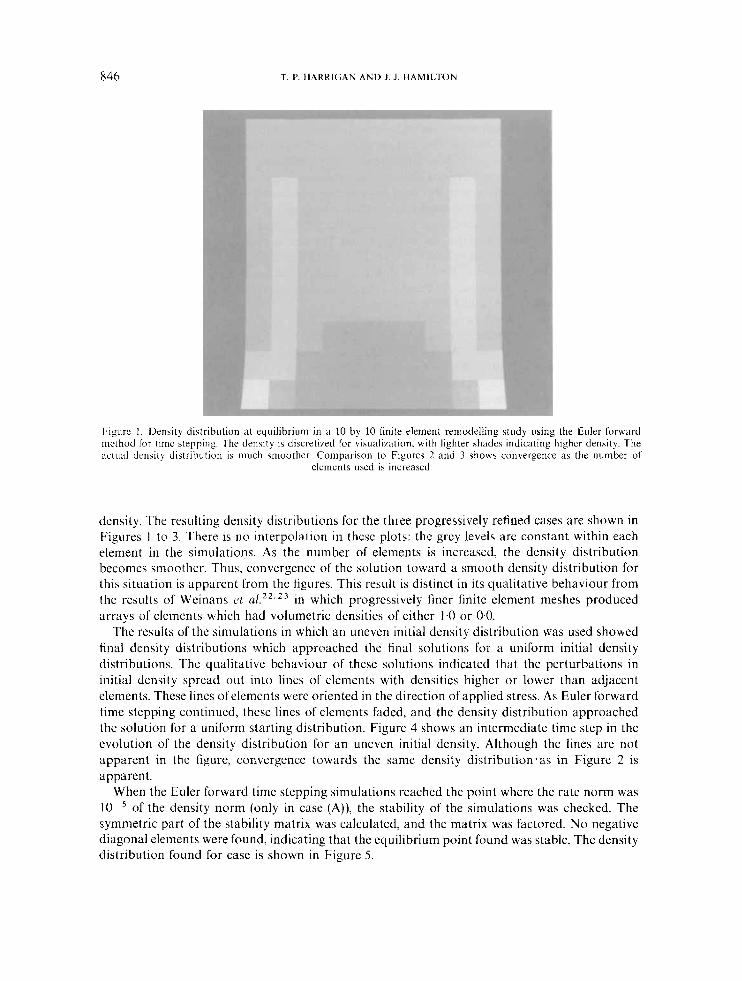
I,.igure I . Density distribution at equilibrium in a 10 by 10 finite element remodelling study using the Etiler forward mcthod for timc stepping. 'l'hc density is discreli7ed for visuali7ation, with lighter shades indicating higher density. The a c ~ u a l density distribution is much smoothcr. Comparison to Figures 2 and 3 shows convergence as the number of

elements used is increased

density. The resulting density distributions for the three progressively refined cases are shown in Figures 1 to 3. There is n o interpolalion in thcsc plots: the grey leveis arc constant within each element in the simulations. As the number of elements is increased, the density distribution becomes smoothcr. Thus, convergence of the solution toward a smooth density distribution for this situation is apparent from the figures. This result is distinct in its qualitative behaviour from the results of Weinans et a l . 2 2 3 2 3 in which progressively finer finite clcment meshes produced arrays of elements which had volumetric densities of either 1-0 or 0.0.

The results of the simulations in which an uneven initial density distribution was used showed final density distributions which approached the tiiial solutions for a uniform initial density distributions. The qualitative behaviour of these solutions indicated that the perturbations in initial dcnsity spread out inlo lines of clcmcnts with dcnsitics highcr or lower Lhan adjaccnt elements. These lines of elements were oriented in the direction of applied stress. As Euler forward time stepping continued, these lines of elements faded, and the density distribution approached the solution for a uniform starting distribution. Figurc 4 shows an intermediate tirnc step in the evolution of the density distribution for an uneven initial density. Although the lines are not apparent in the figure, convergence towards the same density distribution-as in Figure 2 is apparent.

When the Euler forward time stepping simulations reached the point where the rate norm was of the density norm (only in case (A)), the stability of the simulations was checked. The

symmetric part of the stability matrix was calculated, and thc matrix was factored. No negative diagonal elements were found, indicating that the equilibrium point found was stable. The density distribution found for case is shown in Figure 5.

FE SIMULATION OF ADAPTIVE BONE REMODELLING 847

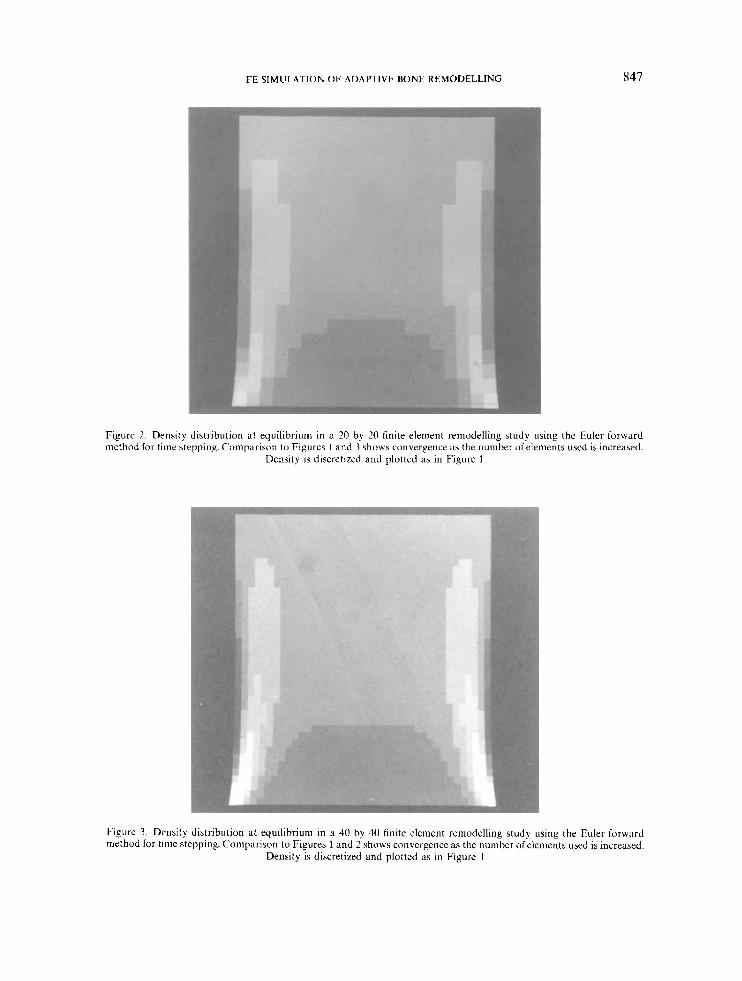
Figure 2. Density distribution at equilibrium in a 20 by 20 finite element remodelling study using the Euler forward method for time stepping. Comparison to Figures I and 3 shows convergence as the number ofelements uscd is increased.

Density is discretized and plotted as i n Figure 1

Figure 3. Density distribution at equilibrium in a 40 by 40 finite element rernodelling study using the Euler forward method for time stepping. Comparison to Figures 1 and 2 shows convergence as the number of clenients used is increased.

Density is discretized and plotted as in Figure 1

848 T. P. HARRIGAN AND J. J . HAMILTON

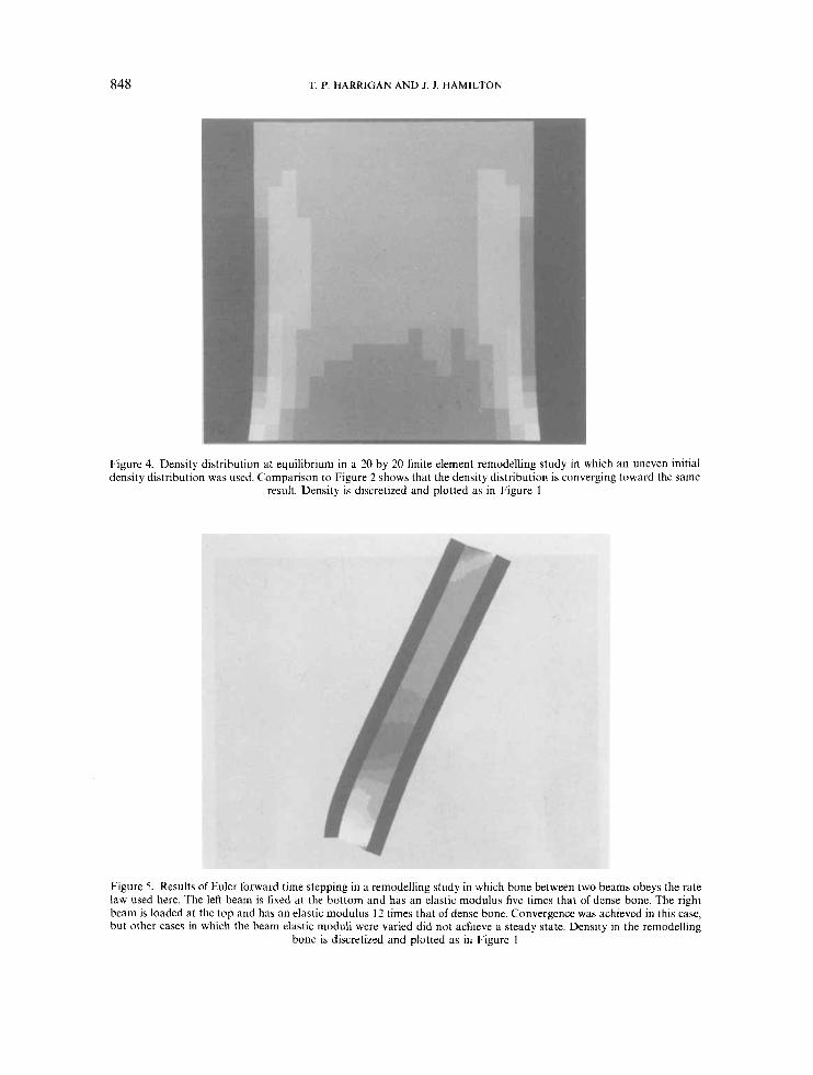
Figure 4. Density distribution at equilibrium in a 20 by 20 finite element remodelling study in which an uneven initial density distribution was uscd. Comparison to Figure 2 shows that the density distribution is converging toward the same

result. Density is discretized and plotted as in Figure 1

Figure 5. Results of Eulcr forward time stepping in a remodelling study in which bone between two beams obeys the rate law used here. The left beam is fixed at the bottom and has an elastic modulus fivc times that of dcnse bone. The right beam is loaded at the top arid has ari elastic modulus 12 times that of dense bone. Convergence was achieved in this case, but other cases in which the beam elastic moduli were varied did not achieve a steady state. Density in the remodelling

bone is discretizsd and plotted as irr Figure 1

Fk SIMULATION OF ADAPTIVE BONE REMODELLING 849

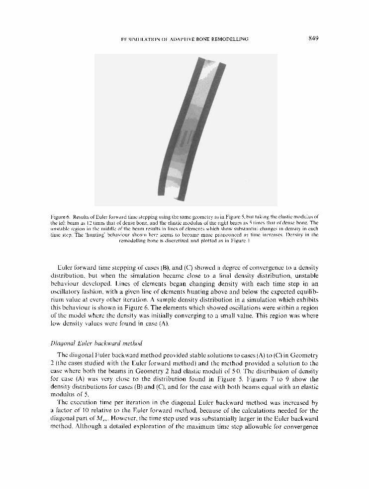
Figure 6. Results of Euler forward time stepping using the same geometry as in Figure 5, hut taking the elastic modulus of the left beam as I ? limes that of dense bone. and the elastic modulus of the right beam as 5 times that of dense bone. The unr;tablc rcgion in rhc middle of the heam results in lines of elements which show suhstantial changes in density in each time step. The 'hunting' behaviour shown here seems to become more pronounced as time increases. Density in the

remodelling hone is discretized and plotted as in Figure I

Euler forward time stepping of cases (B). and (C) showed a degree o f convergence to a density distribution, but when the simulation became close to a final density distribution, unstable bchaviour developed. Lines of elements began changing density with each time step in an oscillatory fashion. with a given line of elements hunting above and below the expected equilib- rium value at every other iteration. A sample density distribution in a simulation which cxhibits this behaviour is shown in Figure 6. The elements which showed oscillations were within a region of the model where the density was initially converging to a small value. This region was where low density values were found in case (A).

D i q o n a l Euler backward method

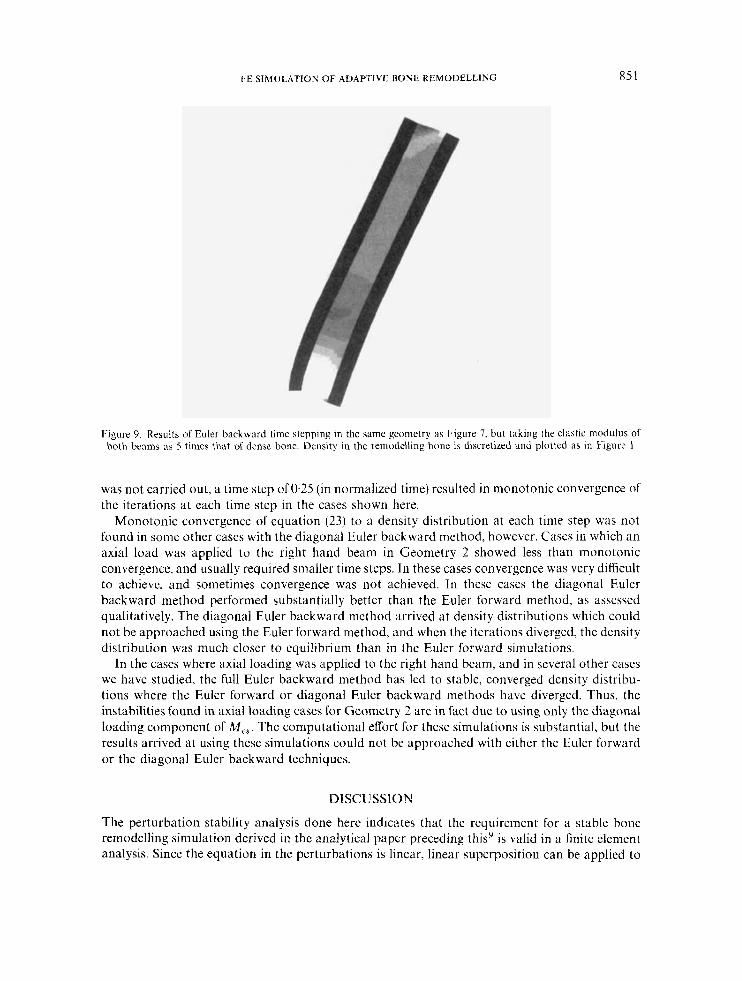
The diagonal Euler backward method provided stable solutions to cases (A) to (C) in Geometry 2 (the cases studied with the Euler forward method) and the method provided a solution to the case where both the beams in Geometry 2 had elastic moduli of 5.0. 'I'hc distribution o f density for case (A) was very close to the distribution found in Figure 5. Figures 7 to 9 show the density distributions for cases (B) and (C), and for the case with both beams equal with an elastic modulus of 5.

The cxccution time per iteration in the diagonal Euler backward method was increased by a factor of 10 relative to the Euler forward method, because of the calculations needed for the diagonal part of M e s . However, the time step used was substantially larger in the Euler backward method. Although a detailed exploration of the maximum time step allowable for convergence

8 50 T. P. HARRIGAN AND J. J. HAMILTON

Figure 7. Results of Euler backward time stepping in the same case as shown in Figure 6 . Note that the density distribution in most rcgions is similar to Figure 6, and that the lines ofclcmcnts arc apparent in thc rcgions of low dcnsity.

Dznsity in the remodelling bone is discretized and plotted as in Figure 1

Figure 8. Results of Euler backward time stcpping in the same geometry as Figure 7, but taking the elastic modulus of both hcams as 12 times that ofdense bone. The Euler hrward time stepping method for this case showed lines of elements

which were similar to h g u r c 6. Density in the remodelling bone is discreti& and plotted as in Figure 1

FE SIMULATION OF ADAPTIVE BONE REMODELLING 851

Figure 9. Results of Euler backward time alepping in the same geometry as Figure 7, but taking the elastic modulus of both beams as 5 times that of dense bone. Density in the remodelling bone is discreti& and ploltcd as in Figure 1

was riot carried out, a time step of 025 (in normalized time) resulted in monotonic convergence of the iterations at each time step in the cases shown here.

Monotonic Convergence of equation (23) to a density distribution at each time step was not found in some other cases with the diagonal Euler backward method, howcvcr. Cases i n which an axial load was applied to the right hand beam in Geometry 2 showed less than monotonic convergence, and usually required smaller time steps. In these cases convergence was very difficult to achieve, and sometimes convergence was not achieved. In these cases the diagonal Euler backward method performed substantially better than the Euler forward method, as assessed qualitatively. The diagonal Euler backward method arrived at density distributions which could not be approached using the Euler forward method, and when the itcrations diverged, the density distribution was much closer to equilibrium than in the Euler forward simulations.

In the cases whcre axial loading was applied to the right hand beam. and in several other cases we have studied, the full Euler backward method has led to stable, converged density distribu- tions where the Euler forward or diagonal Euler backward methods havc divergcd. Thus, the instabilities found in axial loading cases for Geometry 2 are in fact due to using only the diagonal loading component of M e s . The computational effort for these simulations is substantial, but the results arrived at using these simulations could not be approached with either thc Euler forward or the diagonal Euler backward techniques.

DISCUSS I 0 N

The perturbation stability analysis done here indicates that the requirement for a stable bone remodelling simulation derived in the analytical paper preceding this' is valid in a finite element analysis. Since the equation in the perturbations is linear. linear superposition can be applied to

8 52 T. P. HARRIGAN A N D J. J. HAMtLTON

investigate D,, and M,, separately. The equation derived here shows that a negative value for (a -m) is necessary for stability, sincc the matrix D,, is diagonal and every term multiplying (n -m) is positive. This is in agreement with a companion analytic study. Also the diagonal character of D,, agrees with the point-wise instabilities seen analytically with n > m.

In contrast to thc simplc conditions necessary for stability, the conditions which are sufficient for stability are complicated, and seem to depend on the particular structure analysed. We have been unable to find conditions which guarantee negative definiteness in general for the matrix

The diagonal or full Euler backward time stepping algorithm is expensive in terms of computer time, but it allows the calculation of density distributions which are not possible using the Euler forward method. The computations needed are a series of back substitution operations using the factorized stiffness matrix in which each remodelling finite element generates a force vector which is used to solve for a set of displacements. The displacements due to each element force are then used to calculate a change in strain energy within an element due to a stiffness change in another element. The symmctric part of the full matrix A l e , + D,, was Calculated in the stability analysis, and the diagonal part of this matrix was calculated in the diagonal Euler backward method.

The numerical studies and the derivations used here are related specifically to a remodelling rule which is based on strain energy density. Although other remodelling rules exist, and have been studied, we chose to study this rule owing to its mathematical simplicity. This allowed us to concretely develop a prediction for stability which can be used in finite element analyses of remodelling structures.

The asymmetry found in the matrix M e , deserves some comment, since it can be argued that this asymmetry shows that bone remodelling is not an optimal process, at least if it follows this rule. If bone remodelling is an optimal process, then the resulting density distribution is one which minimizes a certain functional with respect to all possible density distributions. If, as in finite element analysis, we discretize the density distribution, then the functional on density becomes a function of the dcnsity at each discretized point within the model. If this ‘potential’ function exists, then the right hand side of equation (7) results from setting a partial derivative equal to Lero. If equation (7) is equivalent to

M e , + D e y ’

then the mixed partial derivatives ought to be equal. That is, if there is a function P which is extremked relative to the density distribution by equation (7), then

(;2P ~- - (PP

Z + e 0 s 0 7 w e

Ales + D,, = M,, + D,, which is not the case. From this point of view, equation (7) is not the result of minimizing a potential function with respect to a dcnsity distribution. In a strict mathematical sense, this bone remodelling rule is not the result of optimizing the density distribution with respect to some sort oi ‘cost’ function.

The density distribution which results from the simulations done in this study can be considered ‘optimal‘ in a certain scnsc, however. If equation (7) IS interpreted as a static or fatigue failure criterion, then it can be said that the material has been arranged so that it is at the strength limit at every point in the structure. Thus, for the specific loads applied to the structure, the

or

IT SIMLLATION OF ADAPTIVE BONE REMODELLING 853

density distribution is at an ‘optimal’ configuration, in some sense. Whether this is the structure which has the minimum weight needed to carry the loads specified (subject to equation (7)) depends on whether the solution is unique.

The solutions obtained here for Euler forward, diagonal Euler backward and full Euler backward agreed to within the convergence tolerances, when convergence was obtained, but we are not able to guarantee uniqueness of thc solutions obtained at this point. Also, since the optimizing characteristics of the remodelling rate equations hare not been fully understood, we can not guarantee path independence for the remodelling equilibrium distributions. Thus, while the simulations here agrcc when arrived at by different paths (Euler forward, diagonal Euler backward and full Euler backward) there is still much to be learned. Even simple bonc rcmodel- ling algorithms such as the one used here are not easily time stepped or understood regarding optimality or solution uniqueness.

The simulation ol bone remodelling is similar to the process of adaptively modifying composite materials in order to minimize weight, but some important differences exist. As in composite design, a resulting structure is sought in which every point of the material studied is at or ncar a defined mechanical statc.’6~iy~21 The method by which the resulting state is achieved is limited in bone remodelling by the processes which change the structure. In bone remodelling, the ‘optimal‘ conditions are only guessed at as yct, and the temporal remodelling processes are simulated, whereas in optimal design of composites, the optimal conditions are usually well known, and there is a wide variety of methods used to arrive at the optimal configuration.

Stability criteria for adaptive changes in density are developed here for a given structure. No criteria are developed to assess the stability of adaptive changes in bone geometry. Cowin‘ has studied the stability of cortical remodelling extensively, but the interaction of geometric and density adaptations remains to be fully assessed.

CONCLUSIONS

A stability criterion for time stepping a particular bone remodelling algorithm is derived in this study, and is explored in two dimensional finite element models. The results indicate that the stability criterion derived is correct. The stability criterion for the density distribution derived ir, a related analytical paper is reflected in the stability requirements seen in this study. Using the finite element method, this study goes further, providing a test which can guarantee the stability of a finite element solution for bone remodelling. This stability guarantee requires a calculation of the converged steady state, however, and can be used in an a posteriori sense only.

Two versions of an Euler backward method for simulating bone remodelling are derived in this paper as well, and both enable us to arrive at equilibrium density distributions which could not be approached with an Euler forward method as implemented here. The diagonal Euler backward method proved superior to the Euler forward method as applied here, and the full Euler backward method has proven to bc a very robust method for bone remodelling simulation.

REFERENCES

1. K. J. Bathe, Finire Elernent Procedures In Engineering Analysis, Prentic-Hall, Englewood Cliffs, N.J.. 1982. 2. G. S. Beaupri-, T. E. Orr and D. R. Cartcr, ‘An approach for timc-dependent hone modeling and remodel-

3 . D. R. Carter, ‘Mechanical loading history and skeletal biology’. ./. Hiomech., 20, 1095--1109 (1987). 4. D. R. Carter and W. C. Hayes, The compressive behavior 01 bone as a two-phase porous structure; J . Bone Joint

5. D. R. Carter, T. E. Orr and D. P. Fhyrie, ‘Relationships between loading history and femoral cancellous hone

ing---Theoretical development’. J . Orihopedic Res., 8, 651 ~ 661 (1990).

Surgery, 59A, 954-962 (1 977).

architecture’, J. Bionirch., 22, 231-244 ( 1 989).

8 54 T. P. HARRIGAN A N D J. .I HAMT1,TON

6.

7. 8.

9.

10.

11.

12. 13.

14.

15. 16. 17.

18.

19.

20. 21.

22.

23.

24.

S. C. Cowin, ‘Mechanical modelling of the stress adaptation process in bone’, Calc$ Tiss. In(., 36, (Suppl. 1) . S98-SI03 (1 984). S. H. Crandall, Engineering Analysis, McGraw-Hill, New York. 1955. D. P. Ehyrie and S. J. Hollistcr? ’Comparison of a trahecular Tissuc strain remodelling theory to experimental results’, Trans. Orthuprdir Res. Soc., 15, 107 (1990). T. P. Harrigan and J. J . Hamilton, ‘An analytical and numerical study of the stability of bone remodelling theories: Dependence on microstructural stimulus’. J. BicJWIeCh.. 25, 477-488 (1992). K. T. Hart and D. T. Davy, ‘Theories of bone modelling and remodelling’, in: S. C. Cowin (ed.). Bone Mechunics, CRC Press, Boca Raton, FL, 1989, pp. 253 277. R. T. Hart. D. T. Davey and K. G. Heiple, ‘A computational method for stress analysis of adaptive elastic materials with a view towards applications in strain-induced hone remodeling’, J . Biomerh. Efig. , 106, 342-350 (1 984). K. Hukkes, Plenary Lecture, First World Congress for Biomechanics, San Diego, 1990. R. Huiskes, €I . Weinans, H. J. Grootenhoer, M. Dalstra, R. Fudala and T. J. Sloof, ‘Adaptive bone rcmodelling theory applied to prosthetic design analysis’, J. Bionirch.. 20, 1135-1150 ( I 987). R. Huiskes, 1% Weinans, B. V. Reitbergen. D. R. Sumner, T. M. Turner and J. 0. Galantc, ‘Validation of strain adaptivc bone-remodelling analysis to predict bone morphology around noncemented TIIA, Orlhopuedic Truns., 15, 399 (1991). P. Lancaster and M. Tismenetsky, 7%e Theory of Matrices, Acadcrnic Prcss, Orlando, FL, 1985. R. A. Meric. ‘Simultaneous material/load/shape variations of thermoelastic structures’, AIA.4 J., 28, 296-302 (1990). T. E. Orr, G. S. Beaupre, D. R. Carter and D. J. Schurman, ‘Computer predictions of bone remodelling around porous-coated implants’, .I. Artl iroplaq, 5, 19 1 - 2 0 (1989). J. C. Rice. S. C. Cowin and J. 4. Bowman, ‘On the dependence or the elasticity and strength of cancellous hone on apparenl densily’, . I . Bionieclz., 21, 1.55-168 (1988). Ci. Sacchi Landriani and M. Rovati, ‘Optimal design for two-dimensional structures madc of composite materials’. J . Eng. Muter. Techno/., 113, 88-92 (1YY1). G. Strang, Inlroduction to Applied ,Mathematics, Wcllesleg-Cambridge Press. Wellesley, MA, 1986. G. N. Vandcrplaats and T. A. Weisshaar, ‘Optimum design of composite structures’, Int. j . nunier. niethods eng., 27, 437-448 (1989). H. Weinans, R. Huiskes and €1. J . Grootenboer, ‘Convergence and uniqueness o f adaptive bonc rcmodelling’, 7ians. Orthopedic Rex Soc.. 14, 31 0 (1 9891. H. Weinans, R. Huiskes and H. J. Grootenboer, ‘Numerical comparisons or strain-adaptive bone remodelling theories’. Truns. First World Congrers of Biomechanics, Vol. 11, 1990, p. 75. J. L. Wolf€, Thi, Law of’Bone Remodelling, Translated by P. Maquet and R. Furlong, Springer-Veriag, Berlin; 1986 (original publication 1982).