Solution-limited time stepping to enhance reliability in CFD ...

Journal of Computational Physics 228 (2009) 4836–4857

Contents lists available at ScienceDirect

Journal of Computational Physics

journal homepage: www.elsevier .com/locate / jcp

Solution-limited time stepping to enhance reliability in CFD applications

Chenzhou Lian *, Guoping Xia, Charles L. MerkleSchool of Mechanical Engineering, Purdue University, ARMS 3142, 701 W. Stadium Ave., West Lafayette, IN 47907-2045, United States

a r t i c l e i n f o

Article history:Received 14 August 2008Received in revised form 25 March 2009Accepted 26 March 2009Available online 7 April 2009

MSC:65B9976M12

Keywords:Computational fluid dynamicsNumerical methodsConvergence and reliability

0021-9991/$ - see front matter � 2009 Elsevier Incdoi:10.1016/j.jcp.2009.03.040

* Corresponding author. Tel.: +1 765 426 8695; faE-mail address: [email protected] (C. Lian).

a b s t r a c t

A method for enhancing the reliability of implicit computational algorithms and decreasingtheir sensitivity to initial conditions without adversely impacting their efficiency is inves-tigated. Efficient convergence is maintained by specifying a large global Courant (CFL)number while reliability is improved by limiting the local CFL number such that the solu-tion change in any cell is less than a specified tolerance. The method requires control overtwo key issues: obtaining a reliable estimate of the magnitude of the solution change anddefining a realistic limit for its allowable variation. The magnitude of the solution change isestimated from the calculated residual in a manner that requires negligible computationaltime. An upper limit on the local solution change is attained by a proper non-dimension-alization of variables in different flow regimes within a single problem or across differentproblems. The method precludes unphysical excursions in Newton-like iterations in highlynon-linear regions where Jacobians are changing rapidly as well as non-physical resultssuch as negative densities, temperatures or species mass fractions during the computation.The method is tested against a series of problems all starting from quiescent initialconditions to identify its characteristics and to verify the approach. The results reveal asubstantial improvement in convergence reliability of implicit CFD applications thatenables computations starting from simple initial conditions without user intervention.

� 2009 Elsevier Inc. All rights reserved.

1. Introduction

Computational algorithms for systems of partial differential equations traditionally use iterative methods to obtainnumerical solutions. The efficiency and reliability of such procedures represent crucial issues for practical applications.An implicit goal of any algorithm is to maximize computational efficiency while minimizing user intervention and thespecification of user defined control variables at input. An ideal algorithm should converge reliably from any physicallymeaningful initial condition while using a standard set of predefined control variables. For example, an ideal time-marchingprocedure would use a fixed Courant (CFL) number for every problem and converge reliably from any easily specified initialcondition to the correct solution without user intervention. Such an ideal is far from conventional experience. Iterativeprocedures are sensitive to initial conditions, are adversely affected by grid stretching and cell aspect ratios and by the non-linearities that are characteristic of fluid mechanics. Issues such as these combine to require significantly different CFL valuesfor various problems and often require changes in CFL during the iteration to preclude divergence and ensure efficiency.Without watchful user intervention, solutions often diverge or ‘blow up’ as nonlinearities cause local Jacobians to drivethe solution in improper directions or produce unrealistic physical variables such as negative temperatures, densities ormass fractions during the iteration.

While convergence acceleration has been the subject of many studies [1–7], methods for ensuring code reliability gener-ally rely upon ad hoc procedures. One common method for enhancing reliability is to add increased artificial dissipation to

. All rights reserved.

x: +1 765 494 0307.

mailto:[email protected]

http://www.sciencedirect.com/science/journal/00219991

http://www.elsevier.com/locate/jcp

Nomenclature

F inviscid flux vectorF v viscous flux vectorH source termsij Reynolds stress tensordij Kronecker deltal molecular viscosityh0 total enthalpyC, Cp matrix coefficientQ conservative transport variablesQp primitive transport variablebQ characteristic transport variables pseudo timeu, v, w Cartesian velocity componentx, y, z Cartesian coordinatei grid point indexCFL Courant–Friedrich–Levy numberA, Ap,i, Ap,v Jacobian matricesq densityp static pressurep0 stagnation pressureT temperatureT0 stagnation temperatureu0, v0, w

0fluctuation of velocity in x, y and z direction

I identity matrixU initial velocity magnitudeRe Reynolds numberb flow angleMa Mach numberDQest

p estimated solution change

DQp solution changeQpref reference variablea max allowable fractional change in solution

C. Lian et al. / Journal of Computational Physics 228 (2009) 4836–4857 4837

the algorithm in the early stages of the computation as, for example, starting with a first-order procedure and then switchingto a higher-order scheme as the solution nears convergence. The first-order algorithm, however, may not be sufficiently dis-sipative to ensure that the initial condition leads to convergence and the choice of when to transition to the desired order ofaccuracy is unknown. Further, even a converged first-order solution may be too far from the final solution to guarantee con-vergence of the higher-order scheme.

A second common procedure for ensuring reliability is to ramp the CFL during the solution process. The iteration is startedfrom a small CFL and increased to an upper limit based on past experience. Again, the starting value, the final value and theallowable rate of increase are all unknown and can vary dramatically from problem to problem. The alternative of usingsmall CFL numbers throughout the iteration, in principle, enhances reliability, but results in inordinately long computationtime. The choice of an a priori CFL schedule, however, remains an open issue and values are generally set arbitrarily as theliterature on optimal strategies for CFL specification is limited [4–7].

A third common procedure is to reset positive-definite variables (such as density or temperature) to a small positive valuewhen computational excursions cause them to change sign. While this action precludes divide checks and NaN’s, such arbi-trary changes often interact adversely with the convergence process requiring increased numbers of iterations. Further,resetting variables does not remove the underlying cause and negative quantities generally reappear in succeeding timesteps.

Often, all three of the above methods are combined with other similar techniques to try to improve code reliability. Amajor limitation is that all are performed in an ‘open-loop’ manner—the correction is devised before the problem appears,and is implemented without regard for why or when the difficulty appears.

The goal of the present article is to investigate a ‘closed-loop’ procedure for improving algorithm reliability that controlsthe local CFL during the iteration on the basis of the convergence process itself rather than by means of an a priori procedure.The method chosen is based upon a concept suggested by Luke et al. [8], but differs from their approach in that it requiresnegligible computational overhead and has been extended to improve its effectiveness. The objectives are to control thechange of all variables at every grid point and iteration in such a manner that a single, pre-specified value of CFL can be used

4838 C. Lian et al. / Journal of Computational Physics 228 (2009) 4836–4857

for all computations while simultaneously reducing sensitivity to initial conditions and grid distribution and ensuring thatnon-physical values are not encountered. The closed-loop control is achieved by specifying a maximum solution change thatallows the code to determine a local CFL in such a manner that this tolerance is not exceeded. Appropriate limits on the frac-tional change of the solution should ensure that the linearization procedure for converting the differential equations to alge-braic form will remain valid so that Newton-based convergence processes do not diverge because of large changes inJacobians and that positive-definite quantities cannot change sign. The approach allows a large CFL in non-sensitive regionsof the convergence process while restricting the CFL in rapidly changing regions. We call this control method the solution-limited time stepping method. Our goal is to demonstrate the characteristics of this automatic method for determining CFLand its impact on code reliability.

In the following sections we first summarize the conservation equations of fluid mechanics along with the representativediscretization procedure that is used for the examples. We then describe the solution-limited time stepping procedure andapply it to a scalar problem and the one-dimensional fluid equations followed by results for a series of problems of increasingdifficulty to assess the effectiveness and generality of the method. We close with a summary of the findings.

2. Governing equations and discretization method

Although the solution-limited time stepping procedure presented here is applicable to any implicit computational algo-rithm, for definiteness we specify the equations of motion and the solution method that are used in the examples. The Na-vier–Stokes equations can be written as:

@Q@sþr � ðF � F vÞ ¼ 0 ð1Þ

where Q = (q, qu, qv, qh0 � p)T is the conservative variables vector, s is a pseudo time used for iterative solution and F andF v are the inviscid and viscous flux vectors that each include three components:

F ¼ E~iþ F~jþ G~k and F v ¼ Ev~iþ Fv

~jþ Gv~k ð2Þ

The inviscid flux vectors are:

E ¼

qu

qu2 þ p

quvquw

quh0

0BBBBBBB@

1CCCCCCCA; F ¼

qvquv

qv2 þ p

qvw

qvh0

0BBBBBBB@

1CCCCCCCA; G ¼

qw

quw

qvw

qw2 þ p

qwh0

0BBBBBBB@

1CCCCCCCA ð3Þ

while the viscous flux vectors are:

Ev ¼

0

sxx

syx

szx

usxx þ vsyx þwszx þ kTx

0BBBBBBB@

1CCCCCCCA; Fv ¼

0

sxy

syy

szy

usxy þ vsyy þwszy þ kTy

0BBBBBBB@

1CCCCCCCA; Gv ¼

0

sxz

syz

szz

usxz þ vsyz þwszz þ kTz

0BBBBBBB@

1CCCCCCCA ð4Þ

The quantities, sij, represent the nine components of the stress tensor:

sij ¼ �23lðux þ vy þwzÞdij þ l @ui

@xjþ @uj

@xi

� �ð5Þ

and, x, y, and z, are the Cartesian coordinates.The conservation equations must be augmented by appropriate constitutive relations for the fluids of interest to obtain a

closed set. A general Gibb’s function, g(p, T) provides a convenient constitutive relation for a broad range of fluids problemsfrom which the density and enthalpy can be found [9]. In addition, the fluid viscosity, l(p, T), and thermal conductivity, k(p,T), are likewise specified as arbitrary functions of pressure and temperature.

Numerical solutions to Eq. (1) require an appropriate discretization procedure and a suitable iterative scheme. We usefinite volume methods to discretize the spatial derivatives and solve the resulting algebraic system by treating the pseu-do-time derivative in Eq. (1) as an iterative variable that can be marched from a selected initial condition to a converged finalresult. Because @Q/@s vanishes as pseudo time goes to infinity and so has no impact on the final solution it can be expressedin non-conservative form without impacting the final solution. Accordingly we use the chain rule to transform from conser-vative variables, Q, to the primitive variables, Qp = (p, u, v, w, T)T so that Eq. (1) becomes:

Cp@Qp

@sþr � ðF � F vÞ ¼ 0 ð6Þ


The pressure and temperature in the primitive variables complement the variables in the constitutive relations while theJacobian matrix, Cp, provides a transformation between Q and Qp. Although the physical Jacobian can be used, both solutionaccuracy and convergence efficiency indicate that artificially defined matrices, Cp, are sometimes preferable. Although suchartificial matrices provide improvements in solution accuracy and convergence in general computations, they can also in-crease sensitivity to initial conditions. The methods described herein decrease sensitivity to initial conditions considerablyfor applications with either physical or artificial pseudo-time coefficients, Cp.

The finite volume discretization of the inviscid and viscous divergence operators is considered separately. The divergenceoperator for the inviscid flux,r � F , can be discretized by central differences [10–12], upwind flux-vector splitting [13–16] orflux-difference splitting [17–19]. Our examples use an upwind, flux-difference splitting method based upon Gauss’ theoremwith the fluxes on each face determined by an approximate Riemann solver. After integrating the continuous divergenceoperator, r � F , over a volume, X, a discrete divergence operator, rD � F , for the inviscid fluxes can be defined as:

rD � F ¼1X

XK

k¼1

12ðF L þ F RÞ �

12

Cp C�1p Ap;i

�� ðQ pR � Q pLÞ� �

kSk ð7Þ

In this expression, the flux Jacobian is defined as Ap;i ¼ @F=@Q p, the vectors, F L and F R, represent the normal components ofthe flux crossing the kth face, and Sk is the face area. The second term in Eq. (7) is an artificial dissipation term introduced in

the approximate Riemann procedure that depends upon the matrices Cp and Ap,i. This matrix Cp C�1p Ap;i

�� must be defined

carefully to ensure a proper amount artificial dissipation. The preconditioning Cp developed by Turkel [20], Van Leer [21],Viviand [22], Briley [23], or Merkle [24] can ensure an appropriate amount of artificial dissipation. The physical matrix Cp

is given by:

Cp ¼

qp 0 0 0 qT

uqp q 0 0 uqT

vqp 0 q 0 vqT

wqp 0 0 q wqT

h0qp � ð1� qhpÞ qu qv qw h0qT þ qhT

0BBBBBB@

1CCCCCCA
For the examples shown below, the physical quantity, qp, in this matrix was replaced by an artificial property term,
q0p ¼ 1V2

p� qT ð1�qhpÞ

qhT, and the preconditioned velocity scale Vp is defined as, Vp ¼min max

ffiffiffiffiffiffiffiffiffiffiffiffiffiffiffiffiffiffiffiffiffiffiffiffiffiffiffiffiu2 þ v2 þw2p

; lqDx ;

lqDy ;

lqDz

� ; c

h i,

where c is the sound speed. Note that the flux Jacobian couples the discretization with the pseudo-time parameter of theiterative procedure.

The divergence operator for the viscous fluxes is discretized by a Galerkin procedure that results in a discrete viscousdivergence operator given as:

rD � F v ¼1X

XK

k¼1

ðF vÞk � Sk ð8Þ

To complete the setup of the iterative procedure we replace the pseudo-time operator in Eq. (6) by an Euler implicit dif-ference and replace the remaining terms by their discrete forms from Eq. (7) to yield the final algebraic system:

CpQkþ1

p � Q kp

Ds¼ �frD � ðF � F vÞgkþ1 ð9Þ

Here, the superscript k represents the running variable in pseudo time.To solve Eq. (9), we linearize the terms on the right side at the new pseudo-time level by Taylor’s series expansions:

ðrD � FÞkþ1 � ðrD � FÞk þrAp;i � DQp ð10aÞ

and

ðrD � F vÞkþ1 � ðrD � F vÞk þrAp;v � DQ p ð10bÞ

where the Jacobians are defined as: Ap;i ¼ @F=@Q p;Ap;v ¼ @F v=@Q p and DQ p � Qkþ1p � Qk

p where the flux Jacobian is defined asAp = Ap,i � Ap,v. Upon rearranging, we obtain the final algebraic system,

I þ DsC�1p ðr � ApÞ

n okDQ p ¼ �Ds C�1

p frD � ðF � F vÞgh ik

ð11Þ

The implicit operator in Eq. (11) is linear but requires a matrix inversion at each pseudo-time step. Because of its wide-banded nature in multi-dimensional problems, it is generally solved by approximate methods such as alternating directionimplicit (ADI) [25,26], point Gauss–Seidel [27–29], line Gauss–Seidel (LGS) [30,31] or GMRES [32]. Here, we use a line Gauss–Seidel method. Because our implementation is based on an unstructured format, a least squares method is used to calculatethe gradients of the primitive variable which are used for the reconstruction on the interface between adjacent cells.


3. The solution-limited time stepping method

As intimated above, large CFL values are needed to ensure efficient convergence, but small CFL’s are needed to ensure reli-able convergence. In general, larger CFL’s can be used as the iteration nears convergence, while smaller values are imperativewhen it is far from the final solution. An important aspect of controlling solution reliability without adversely impacting effi-ciency is to recognize that at a given time in the iteration, some portions of the flowfield will be changing rapidly (and, hence,will need careful protection against divergence and unphysical results) while other portions are changing slowly (andaccordingly can and should be advanced aggressively). The goal of the present work is to devise a means for monitoringthe solution change at every grid point and every step in an effort to determine local CFL values that maximize the progresstoward convergence while simultaneously minimizing the likelihood of divergence. The method involves two importantconcepts: first, an efficient means must be identified for estimating how large the solution change will be, and second, anacceptable magnitude for the allowable solution change must be established. These two items are discussed separatelybelow.

3.1. The estimated solution change

An efficient estimate of the manner in which the solution change, DQp, varies with the local time step size is imperative.Defining acceptable values of Ds at each grid point by computing a series of implicit time steps is computationally intrac-table since the preferred Ds values will be different at every grid point and the change at any grid point will be dependent onthe change at neighboring cells as well as local values. Following the general spirit of the method suggested by Luke et al. [8],we set the estimated solution change (which we designate as DQest

p ) equal to the residual of the implicit update relation in Eq.(11):

DQestp ¼ �Ds C�1

p frD � ðF � F vÞgh ik

ð12Þ

Thus, DQestp is obtained by omitting the divergence terms on the left side of Eq. (11) and is identical to the update relation that

would be obtained from an Euler explicit discretization of Eq. (6). Because the residual must be computed as part of the im-plicit algorithm, the computation of DQest

p requires no additional manipulations or iterations. Thus, in contrast to the proce-dure used by Luke et al. [8] whose procedure required two iterations and was relatively expensive to employ, our estimatehas a negligible impact on the overall CPU time.

The estimated solution change in Eq. (12) is proportional to the time step, Ds. Consequently, for any cell in which DQestp is

deemed large enough to cause convergence difficulties, the local time step is reduced to bring DQ estp to an acceptable mag-

nitude. This time-step-limiting procedure will be useful only to the extent that DQ estp provides a reasonable bound on DQp.

The adequacy of this estimate must be verified, but as a first step in this direction, we compare relative magnitudes of DQestp

and DQp by combining Eqs. (11) and (12) to obtain:

DQestp ¼ I þ DsC�1

p ðrD � ApÞn ok

DQ p ð13Þ

For small pseudo-time steps, Ds, the second term in the brackets are negligible and the actual calculated and estimated solu-tion changes are approximately equal, DQest

p � DQ p. For large Ds, the estimated change, DQ estp , increases linearly without

bound (see Eq. (12)) whereas the actual change, DQp, approaches a constant value. The behavior at these two limits suggeststhat the estimated solution change may serve as a nominal upper bound on the calculated change for all D s and that thenorm of DQp is bounded by the norm of DQ est

p . This supposition must however be verified. In Section 4, we use both analyticaland numerical methods to demonstrate the effectiveness of DQ est

p as a useful estimator of the calculated solution change,DQp.

3.2. Setting the allowable solution change

As a formal procedure for defining the allowable magnitude of the solution change we introduce a reference vector, Qrefp

and a scalar multiplier, a. We then limit the local pseudo-time step in such a manner that the estimated solution change,DQest

p , will be less than the product of a and Qrefp :

DQ estp

�� 6 aQ refp ð14Þ

This limit is to be applied to each variable at each grid point with the local time step being chosen to satisfy the most restric-tive variable. The effectiveness of Eq. (14) depends upon defining appropriate values for both the reference vector and thescalar multiplier. If the method is to be useful, it is imperative that the definitions for both these quantities be applicableover widely varying flow regimes.

Picking a value for a is quite straightforward, whereas the reference quantities require more consideration. For positive-definite quantities such as pressure, density or temperature that are not allowed to change sign, positivity is ensured bychoosing a less than unity. For example, restricting the solution to a 10% change (a = 0.1) will ensure positivity, while also


eliminating strong non-linear effects in Newton-based iteration procedures by precluding large changes in Jacobians fromstep to step while still enabling efficient convergence. Because Dp and DT are only estimates of the change, sign changesare still possible but small values of a provide a substantial margin of safety and we have not observed sign changes fora wide variety of problems.

Indefinite variables such as velocity that must be allowed to change sign require a scaling factor greater than unity, or areference value larger than that in the local cell. As discussed below, our results have shown that pressure is the most sen-sitive variable, whereas velocity is relatively insensitive.

Having defined representative values for the scaling constant, a, we next consider methods for defining the referencevariables with special emphasis on the pressure.

3.3. Scaling the reference variables

The reference vector, Q refp , should be based upon local conditions in the computational domain as defined by the current

iteration. A first choice is to set the reference vector for any cell equal to the current solution vector in that cell, Qrefp ¼ Q n

p;k,where k refers to the local cell, and n refers to the present time step. Of the pressure, velocity and temperature, the pressurechange is more sensitive and requires more care because the pressure gradient, rather than the pressure, appears in theequations of motion. For example, in incompressible flows, the thermodynamic pressure clearly would not serve as anappropriate reference variable. Thus, while the reference value for determining the maximum allowable pressure changeshould depend upon the local pressure in the given cell, this local solution must be scaled appropriately to incorporatethe local flow physics in a proper manner. Improper normalization can allow solution changes that are too large (thus allow-ing divergence) or too small (thereby slowing convergence).

The reference pressure must be determined from the local pressure gradient which can be estimated from the momentumequation with a pseudo-time term added to represent the iterative procedure. The pressure gradient depends upon flowcharacteristics such as the local Mach number, the local Reynolds number, the local acceleration or the local body forcesand is essentially independent of the magnitude of the thermodynamic pressure. A properly defined reference pressureshould reflect these several variations in flow characteristics in a manner that is representative of the local physics. Usingthe one-dimensional momentum equation as an example,

q@u@sþ @qu2

@xþ @p@x¼ l @

2u@x2 þ qg ð15Þ

it is immediately seen that multiple terms can balance the pressure gradient. Pertinent scaling variables can be obtainedfrom formal perturbation expansion methods [33]. For brevity, we here simply tabulate pertinent scalings in the represen-tative limits.

For high Reynolds number flows, the convective term balances the pressure gradient, and the pressure change scales asthe local dynamic pressure resulting in the reference pressure pref = qu2. At low Reynolds numbers, the pressure gradient isbalanced by viscous forces and the pertinent reference pressure is the local shear stress, pref = sij. For problems dominated bybuoyancy or body force terms, the reference pressure depends upon the gravitational term, pref = qgh. Finally, the pressurechange can be determined by local gradients in the solution giving rise to a reference pressure, pref = Dp, where Dp representsthe pressure gradient across the local cell. In a general computation, using the local reference pressure as the largest of theseseveral values along with a choice of a less than unity, ensures small changes in the Jacobians and precludes sign changes inthe pressure.

An appropriate reference temperature is generally somewhat easier to identify than the pressure. Like pressure, the ther-modynamic temperature cannot change sign. In solutions attempted to date, using the local thermodynamic temperature asthe reference condition has proven sufficient to ensure both positivity and insensitivity to initial conditions. Nevertheless,problems for which the local temperature gradient must also be included might be encountered. As a special check on tem-perature scaling, we have included an example in which the flowfield contains substantial amounts of heat transfer (the tem-perature changes by an order of magnitude) as noted later. Ensuring that pressure and temperature are positive and thattheir changes are restricted to a small fraction of their previous values also ensures that the density remains well-behaved.

The reference velocity is somewhat different in that the velocity must be allowed to change sign. The reference velocitycan be based upon the local velocity in a given cell or upon a velocity change imposed by a pressure gradient across the cellas determined by the Method of Characteristics (MOC). For the former limit, we set uref ¼

ffiffiffiffiffiu2

i

qfor each local cell, while for

the latter, we have, uref = cDp/cp. The MOC procedure clearly can lead to velocity changes. Accordingly, we take a = 0.1 for theMOC limit, and a = 2 for the local velocity limit to allow it change sign in non-zero velocity regions. However, regions inwhich the velocity is large, the local velocity limit may have little effect, but a carefully defined pressure limit appears tobe sufficient to protect the solution change in such regions. To circumvent difficulties in cells in which the reference velocityis identically zero by either of these conditions, we have imposed a third reference velocity as 10�9 times some easily iden-tifiable characteristic velocity in the global flowfield. Thus, for the velocity components, ui, in cell k, we limit

jDui;kj 6 2ffiffiffiffiffiffiffiffiffiffiffiffiffiffiffiffiffiffiffiffiffiffiffiffiffiffiffiffiffiffiffiffiffiffiu2

1;k þ u22;k þ u2

3;k

q. Representative solutions given later critically test this limit by starting with initial conditions

in which the entire velocity field is set to zero and the pressure is uniform. This proves to be a rather conservative limit whenthe velocity components are small, but as the solution approaches convergence (or for initial conditions where the velocity is


large) it can be overly lenient and allow large fluctuations in the Jacobians. The special attention to the pressure limit, how-ever, offsets this wider limit on the velocity components and we have found this method to be successful in all solutions todate. The present paper also includes examples containing recirculation regions behind a backward facing step and heataddition in a pipe flow starting from rest to test for difficulties when the local velocity passes through zero during the iter-ation. Other computations (not included) based upon using a global characteristic velocity as the reference speed with thevalue of a set equal to 0.1 as for a positive-definite variable have also proven effective for applications in which such a veloc-ity is easily discerned.

3.4. Summary of solution-limited time stepping procedure

The purpose of the limiting procedure is to define a local time step, Ds, at every grid point such that DQ estp

�� 6 aQ refp . As

shown next, this limit effectively ensures that the L2-norm of the calculated solution change will be bounded by a similarcondition, jDQ pj 6 aQ ref

p . Since DQestp is equal to the residual of the implicit algorithm, it is already computed as a part of

the calculated solution, and therefore requires negligible CPU resources. We implement the solution-limited time steppingmethod in the following manner:

1. Specify a global Courant number, CFLspecified, that is large enough to provide efficient convergence in the limit as the solu-tion approaches convergence. (The value used in the examples is CFLspecified = 1000.) The CFL is defined as:

CFL ¼ k � DtDl

where k is the maximum eigenvalue of the convective Jacobian, Dl is the longest dimension of the cell and Dt is the timestep.

2. Choose the reference quantities, Q refp , based upon local conditions: !

pref ¼maxqu2

2;luiDxi

Dx2j

;qgh;Dp;pglobal � 10�9

uref ¼ maxffiffiffiffiffiu2

i

q;cc

Dpp;10�9 � Vglobal

� �Tref ¼ T

where Vglobal is some global velocity chosen to ensure uref is always greater than zero and pglobal is some global referencepressure chosen to ensure pref is always greater than zero.

3. Set the maximum allowable fractional change, a (we have used a = 0.1 for all variables except the velocity change basedon the local velocity where we have used a = 2).

4. Compute the residual of the implicit algorithm in Eq. (11) which gives the estimated solution change, DQestp as noted in Eq.

(12).5. Compare DQ est

p at every grid point with the allowable solution change, aQ refp , and for those cells that exceed the limit,

decrease the local Courant number according to: CFLallowable ¼ CFLspecifiedaQ refp

.DQest

p

�� . This limiting step takes advantage

of the linearity of DQ estp with Ds and is to be done for each component of Qp with the minimum CFL being selected.

6. Use the resulting sequence of Courant numbers to compute the calculated solution change, DQp, and complete the timestep.

It is important to use the time step limiting procedure for every variable at every iteration and every cell in the compu-tation, starting from the initial condition. The local pseudo-time step at every cell and grid point is based upon the smallestDs from all variables. As shown later, the limiting procedure is typically operative over small portions of the flowfield duringlimited parts of the convergence process. As the computation progresses, the entire field can typically be advanced at theglobal Courant number.

4. Bounding assessment of calculated and estimated solution changes

To understand the effectiveness of the estimated solution change as a bound for the implicit calculated change, we firstlook at solution changes for a scalar wave equation, and then for a one-dimensional vector system to compare the estimatedsolution change with the actual solution change.

4.1. Scalar wave equation

As a first step, we consider the calculated and estimated solution changes for the scalar wave equation,

@u@sþ a

@u@x¼ 0 ð16Þ

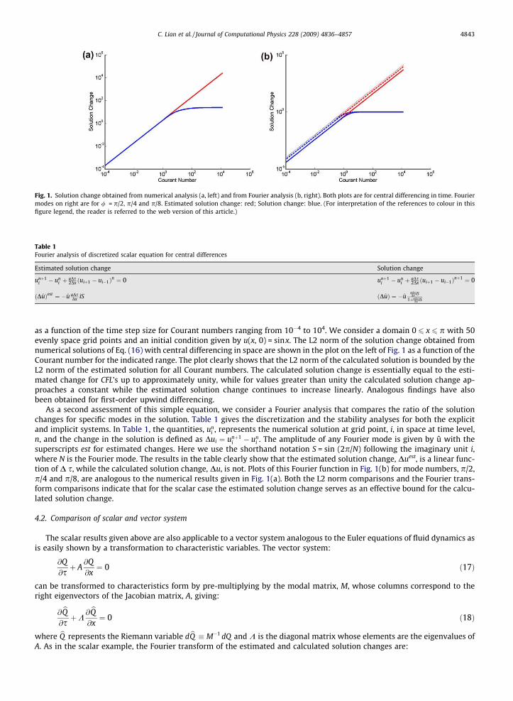
Fig. 1. Solution change obtained from numerical analysis (a, left) and from Fourier analysis (b, right). Both plots are for central differencing in time. Fouriermodes on right are for / = p/2, p/4 and p/8. Estimated solution change: red; Solution change: blue. (For interpretation of the references to colour in thisfigure legend, the reader is referred to the web version of this article.)

Table 1Fourier analysis of discretized scalar equation for central differences

Estimated solution change Solution change

unþ1i � un

i þ aDs2Dx ðuiþ1 � ui�1Þn ¼ 0 unþ1

i � uni þ aDs

2Dx ðuiþ1 � ui�1Þnþ1 ¼ 0

ðDuÞest ¼ �u aDsDx iS ðDuÞ ¼ �u

aDsDx iS

1þaDsDx iS


as a function of the time step size for Courant numbers ranging from 10�4 to 104. We consider a domain 0 6 x 6 p with 50evenly space grid points and an initial condition given by u(x, 0) = sinx. The L2 norm of the solution change obtained fromnumerical solutions of Eq. (16) with central differencing in space are shown in the plot on the left of Fig. 1 as a function of theCourant number for the indicated range. The plot clearly shows that the L2 norm of the calculated solution is bounded by theL2 norm of the estimated solution for all Courant numbers. The calculated solution change is essentially equal to the esti-mated change for CFL’s up to approximately unity, while for values greater than unity the calculated solution change ap-proaches a constant while the estimated solution change continues to increase linearly. Analogous findings have alsobeen obtained for first-order upwind differencing.

As a second assessment of this simple equation, we consider a Fourier analysis that compares the ratio of the solutionchanges for specific modes in the solution. Table 1 gives the discretization and the stability analyses for both the explicitand implicit systems. In Table 1, the quantities, un

i , represents the numerical solution at grid point, i, in space at time level,n, and the change in the solution is defined as Dui ¼ unþ1

i � uni . The amplitude of any Fourier mode is given by û with the

superscripts est for estimated changes. Here we use the shorthand notation S = sin (2p/N) following the imaginary unit i,where N is the Fourier mode. The results in the table clearly show that the estimated solution change, Duest, is a linear func-tion of D s, while the calculated solution change, Du, is not. Plots of this Fourier function in Fig. 1(b) for mode numbers, p/2,p/4 and p/8, are analogous to the numerical results given in Fig. 1(a). Both the L2 norm comparisons and the Fourier trans-form comparisons indicate that for the scalar case the estimated solution change serves as an effective bound for the calcu-lated solution change.

4.2. Comparison of scalar and vector system

The scalar results given above are also applicable to a vector system analogous to the Euler equations of fluid dynamics asis easily shown by a transformation to characteristic variables. The vector system:

@Q@sþ A

@Q@x¼ 0 ð17Þ

can be transformed to characteristics form by pre-multiplying by the modal matrix, M, whose columns correspond to theright eigenvectors of the Jacobian matrix, A, giving:

@ bQ@sþK

@ bQ@x¼ 0 ð18Þ

where bQ represents the Riemann variable dbQ � M�1 dQ and K is the diagonal matrix whose elements are the eigenvalues ofA. As in the scalar example, the Fourier transform of the estimated and calculated solution changes are:


DbQ est ¼ �iSKDsDxbQ ð19Þ

DbQ ¼ � I þ iSKDsDx

� ��1

iSKDsDxbQ ð20Þ

Since the matrix K in Eq. (18) is a diagonal matrix, the scalar analyses of Section 4.1 are also valid for each component of thecharacteristic variable, bQ , so the conclusion that the L2 norm of the calculated solution is bounded by the L2 norm of theestimated solution continues to hold for a system of equations.

Because the magnitude of the calculated solution change is not absolutely bounded by the estimated solution change butonly by its L2 norm, there could (and will) be points in the domain for which the estimated change is identically zero whilethose for the calculated change are finite. This specific point is addressed in the following examples by using problems with auniform initial condition throughout the domain except for a step change at the boundary. The estimated solution change isidentically zero for all grid points except those adjacent to the boundary (the effect of the boundary condition propagatesonly one cell per time step), while the calculated solution change extends over the entire domain (boundary condition effectspropagate over multiple cells in implicit scheme). Thus, in every example, we deal with multiple points for which the cal-culated solution change exceeds the estimated solution change, but the estimator still provides an effective limit on theiteration.

5. Results

To demonstrate the solution-limited time stepping procedure, we start with a simple, one-dimensional problem to testthe general concept and assess its behavior. Following this, we present a series of multi-dimensional examples with an addi-tional physical concept added in each problem to assess its effectiveness in various flow regimes. The initial condition for allcases sets the velocity at all cells in the field to zero and the pressure and temperature to a constant value. The initial densityat every grid point is then obtained from the equation of state. Upstream boundary conditions typically correspond to a spec-ified stagnation pressure, p0, and temperature, T0, and the flow angle. The downstream boundary condition is a specified backpressure, pback. This initial condition is easy to define, simple to implement and broadly useful for a wide variety of problems.

5.1. One-dimensional inviscid flow

As the first step in developing the method, we consider the one-dimensional flow of a perfect gas in a constant area pas-sage. The converged solution for this problem is a trivial uniform flow but it provides a useful first test of the method. Theupstream boundary conditions were chosen as: p0 = 1.4e5 Pa and T0 = 400 K and a series of back pressures were imposedsuch that the Mach number of the converged flow ranged from low subsonic to supersonic speeds. The global CFL was setto 1000 for all cases and the limiting procedure was used to control the local CFL to see if it would respond appropriatelyto the initial condition and provide reliable convergence. There were 100 uniformly distributed cells in the domain. Thegeometry and flow conditions are shown in Fig. 2.

Two sets of constant values were used for the initial condition on pressure. In one case, the initial pressure was set equalto the upstream stagnation pressure while in the second it was set to the back pressure. With the first initial condition, theoutflow boundary is exposed to the back pressure at the first time step and the iterative procedure is initiated by an expan-sion fan propagating into the computational domain from the downstream boundary in pseudo time. We refer to this as anexpansion-initiated case. With the second initial condition, the upstream cell is exposed to the stagnation pressure at thefirst time step and the convergence process starts from a shock wave propagating through the flowfield. We describe thisas the shock-initiated case. In all cases the initial velocity was set to zero and the temperature was set to the upstream stag-nation value.

As a first step, we look in detail at the initial condition and the first several iterative steps using the expansion-initiatedcase as an example. From the initial condition, the velocity in all cells is zero and the pressure is equal to the upstream stag-nation value at every cell except the last one which is equal to the back pressure. The estimated solution change returns amachine zero for Dpest for all cells except the last which returns a finite value. In the companion two-dimensional version ofthis problem (discussed below), the value of Dpest for the entire downstream column of cells was finite, while the Dpest for allremaining cells were round-off zero rather than a machine zero. For this reason, the final limiting terms was added to pref

definition and the reference pressure for all but the last cell was chosen as the nominal value, 10�9pglobal where pglobal

was chosen as the stagnation pressure. The reference pressure in the last cell was limited by the pressure change acrossthe cell, Dp (which in this case was p0 � pback). The corresponding reference velocity was 10�9Vglobal for all but the last cellwhere the reference velocity was set by the MOC limit. In performing the limiting procedure, the Courant number was

Fig. 2. Geometry and boundary conditions for constant area duct.

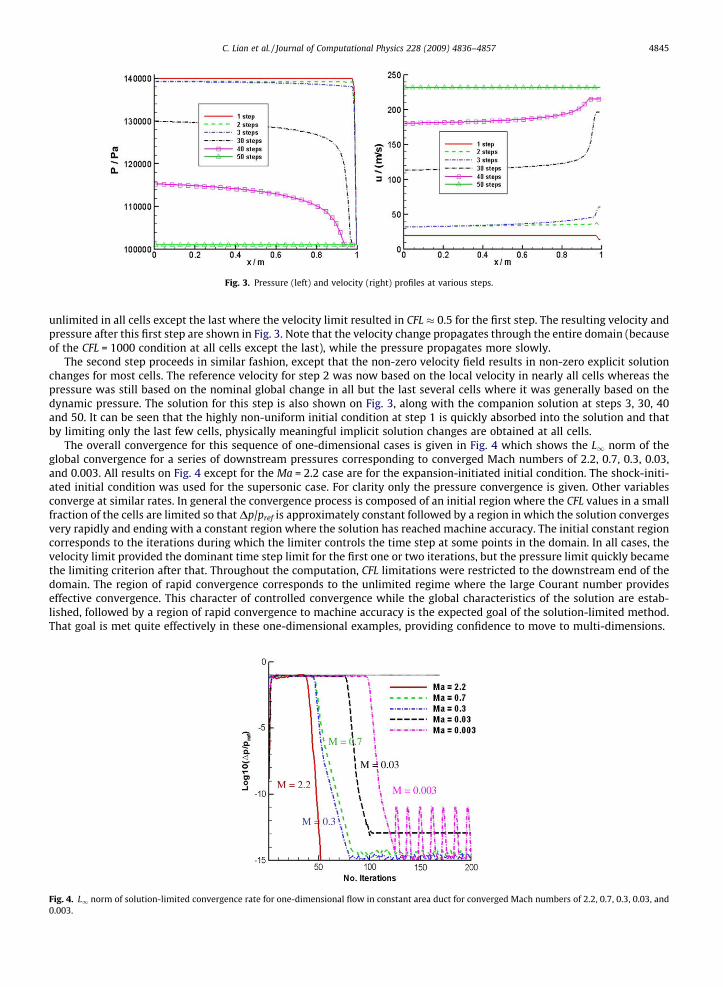
Fig. 3. Pressure (left) and velocity (right) profiles at various steps.


unlimited in all cells except the last where the velocity limit resulted in CFL � 0.5 for the first step. The resulting velocity andpressure after this first step are shown in Fig. 3. Note that the velocity change propagates through the entire domain (becauseof the CFL = 1000 condition at all cells except the last), while the pressure propagates more slowly.

The second step proceeds in similar fashion, except that the non-zero velocity field results in non-zero explicit solutionchanges for most cells. The reference velocity for step 2 was now based on the local velocity in nearly all cells whereas thepressure was still based on the nominal global change in all but the last several cells where it was generally based on thedynamic pressure. The solution for this step is also shown on Fig. 3, along with the companion solution at steps 3, 30, 40and 50. It can be seen that the highly non-uniform initial condition at step 1 is quickly absorbed into the solution and thatby limiting only the last few cells, physically meaningful implicit solution changes are obtained at all cells.

The overall convergence for this sequence of one-dimensional cases is given in Fig. 4 which shows the L1 norm of theglobal convergence for a series of downstream pressures corresponding to converged Mach numbers of 2.2, 0.7, 0.3, 0.03,and 0.003. All results on Fig. 4 except for the Ma = 2.2 case are for the expansion-initiated initial condition. The shock-initi-ated initial condition was used for the supersonic case. For clarity only the pressure convergence is given. Other variablesconverge at similar rates. In general the convergence process is composed of an initial region where the CFL values in a smallfraction of the cells are limited so that Dp/pref is approximately constant followed by a region in which the solution convergesvery rapidly and ending with a constant region where the solution has reached machine accuracy. The initial constant regioncorresponds to the iterations during which the limiter controls the time step at some points in the domain. In all cases, thevelocity limit provided the dominant time step limit for the first one or two iterations, but the pressure limit quickly becamethe limiting criterion after that. Throughout the computation, CFL limitations were restricted to the downstream end of thedomain. The region of rapid convergence corresponds to the unlimited regime where the large Courant number provideseffective convergence. This character of controlled convergence while the global characteristics of the solution are estab-lished, followed by a region of rapid convergence to machine accuracy is the expected goal of the solution-limited method.That goal is met quite effectively in these one-dimensional examples, providing confidence to move to multi-dimensions.

Fig. 4. L1 norm of solution-limited convergence rate for one-dimensional flow in constant area duct for converged Mach numbers of 2.2, 0.7, 0.3, 0.03, and0.003.


5.2. Two-dimensional inviscid flow in constant area channel

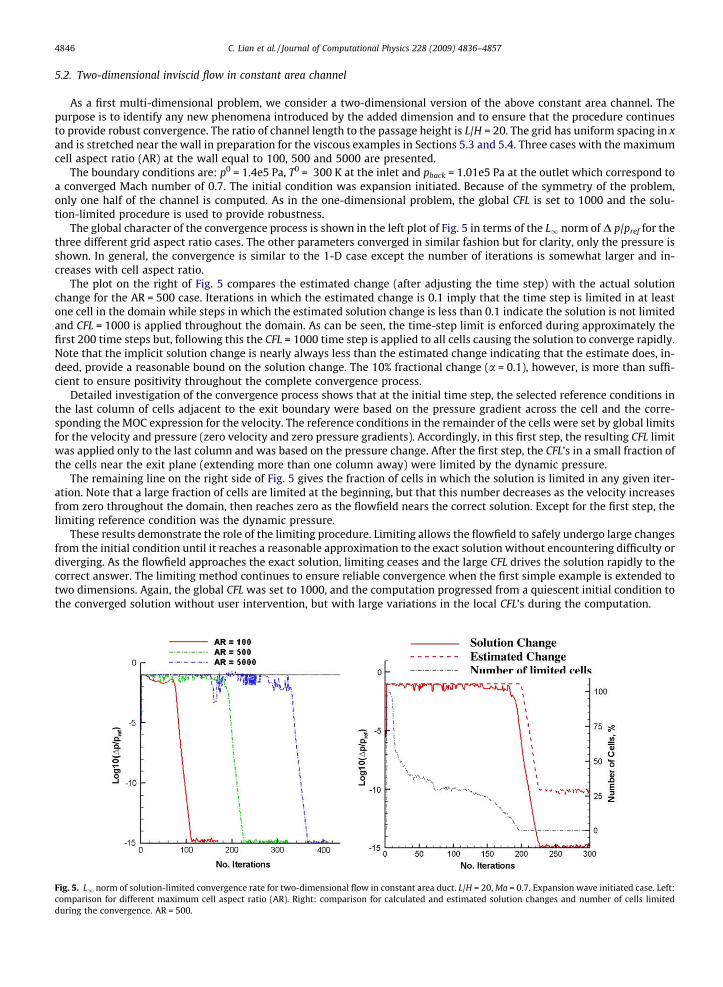
As a first multi-dimensional problem, we consider a two-dimensional version of the above constant area channel. Thepurpose is to identify any new phenomena introduced by the added dimension and to ensure that the procedure continuesto provide robust convergence. The ratio of channel length to the passage height is L/H = 20. The grid has uniform spacing in xand is stretched near the wall in preparation for the viscous examples in Sections 5.3 and 5.4. Three cases with the maximumcell aspect ratio (AR) at the wall equal to 100, 500 and 5000 are presented.

The boundary conditions are: p0 = 1.4e5 Pa, T0 = 300 K at the inlet and pback = 1.01e5 Pa at the outlet which correspond toa converged Mach number of 0.7. The initial condition was expansion initiated. Because of the symmetry of the problem,only one half of the channel is computed. As in the one-dimensional problem, the global CFL is set to 1000 and the solu-tion-limited procedure is used to provide robustness.

The global character of the convergence process is shown in the left plot of Fig. 5 in terms of the L1 norm of D p/pref for thethree different grid aspect ratio cases. The other parameters converged in similar fashion but for clarity, only the pressure isshown. In general, the convergence is similar to the 1-D case except the number of iterations is somewhat larger and in-creases with cell aspect ratio.

The plot on the right of Fig. 5 compares the estimated change (after adjusting the time step) with the actual solutionchange for the AR = 500 case. Iterations in which the estimated change is 0.1 imply that the time step is limited in at leastone cell in the domain while steps in which the estimated solution change is less than 0.1 indicate the solution is not limitedand CFL = 1000 is applied throughout the domain. As can be seen, the time-step limit is enforced during approximately thefirst 200 time steps but, following this the CFL = 1000 time step is applied to all cells causing the solution to converge rapidly.Note that the implicit solution change is nearly always less than the estimated change indicating that the estimate does, in-deed, provide a reasonable bound on the solution change. The 10% fractional change (a = 0.1), however, is more than suffi-cient to ensure positivity throughout the complete convergence process.

Detailed investigation of the convergence process shows that at the initial time step, the selected reference conditions inthe last column of cells adjacent to the exit boundary were based on the pressure gradient across the cell and the corre-sponding the MOC expression for the velocity. The reference conditions in the remainder of the cells were set by global limitsfor the velocity and pressure (zero velocity and zero pressure gradients). Accordingly, in this first step, the resulting CFL limitwas applied only to the last column and was based on the pressure change. After the first step, the CFL’s in a small fraction ofthe cells near the exit plane (extending more than one column away) were limited by the dynamic pressure.

The remaining line on the right side of Fig. 5 gives the fraction of cells in which the solution is limited in any given iter-ation. Note that a large fraction of cells are limited at the beginning, but that this number decreases as the velocity increasesfrom zero throughout the domain, then reaches zero as the flowfield nears the correct solution. Except for the first step, thelimiting reference condition was the dynamic pressure.

These results demonstrate the role of the limiting procedure. Limiting allows the flowfield to safely undergo large changesfrom the initial condition until it reaches a reasonable approximation to the exact solution without encountering difficulty ordiverging. As the flowfield approaches the exact solution, limiting ceases and the large CFL drives the solution rapidly to thecorrect answer. The limiting method continues to ensure reliable convergence when the first simple example is extended totwo dimensions. Again, the global CFL was set to 1000, and the computation progressed from a quiescent initial condition tothe converged solution without user intervention, but with large variations in the local CFL’s during the computation.

Fig. 5. L1 norm of solution-limited convergence rate for two-dimensional flow in constant area duct. L/H = 20, Ma = 0.7. Expansion wave initiated case. Left:comparison for different maximum cell aspect ratio (AR). Right: comparison for calculated and estimated solution changes and number of cells limitedduring the convergence. AR = 500.


As the next step, we impose a no-slip condition on the duct walls and look at the effectiveness of the limiting method inthe presence of viscosity in the entry region of a channel.

5.3. Viscous flow in constant area channel

To investigate the effect of viscous terms on the limiting procedure, we consider developing flow in a channel using thesame geometry as for the above inviscid example. To resolve the boundary layers in the entry region the grid is stretched inboth the axial and radial directions (the radial stretching is the same as that used in the inviscid solution) with a total grid of32,000 cells and a maximum aspect ratio of 500. The channel length to passage height ratio is again, L/H = 20 and the Rey-nolds number is set at 1000. The estimated entry length [34] for this problem is L/H = 44.2, indicating that the boundary lay-ers should grow to a reasonable fraction of the channel in the domain but should not reach the fully developed state. Theboundary conditions chosen for this problem are identical to the conditions that resulted in Ma = 0.7 flow in the above case,specifically: p0 = 1.4e5 Pa, T0 = 300 K at the inlet and pback = 1.01e5 Pa at the outlet. The problem was again started from restwith an expansion wave from the downstream end. Again, the single user-specified quantity for this calculation wasCFL = 1000.

A graphical description of the convergence and limiting process for this viscous problem is given in Fig. 6 showing quan-tities analogous to those for the inviscid problem in Fig. 5. For the viscous problem, the solution change was limited forapproximately the first 150 steps after which it converged rapidly toward the solution. The solution change was generallyless than the estimated change, and never exceeded it by more than a few percent. During the computation, the numberof limited cells increased from the last row of cells in the first step to a maximum and then decreased to zero as a meaningfulflowfield was established. The primary difference was that the reference pressure was sometimes based upon the viscousterm instead of the dynamic pressure, reflecting the different physics in the near-wall regions of the domain. All in all, thiscomputation also converged reliably from the initial quiescent condition to the final converged solution which is shown inFig. 7 for reference.

Fig. 6. L1 norm of solution-limited convergence rate for viscous flow in entry region of channel. L/H = 20, Re = 1000, Expansion wave initiated.

Fig. 7. Converged velocity contours in channel (top) and velocity profiles at various locations (bottom).


5.4. Viscous flow with strong heat addition

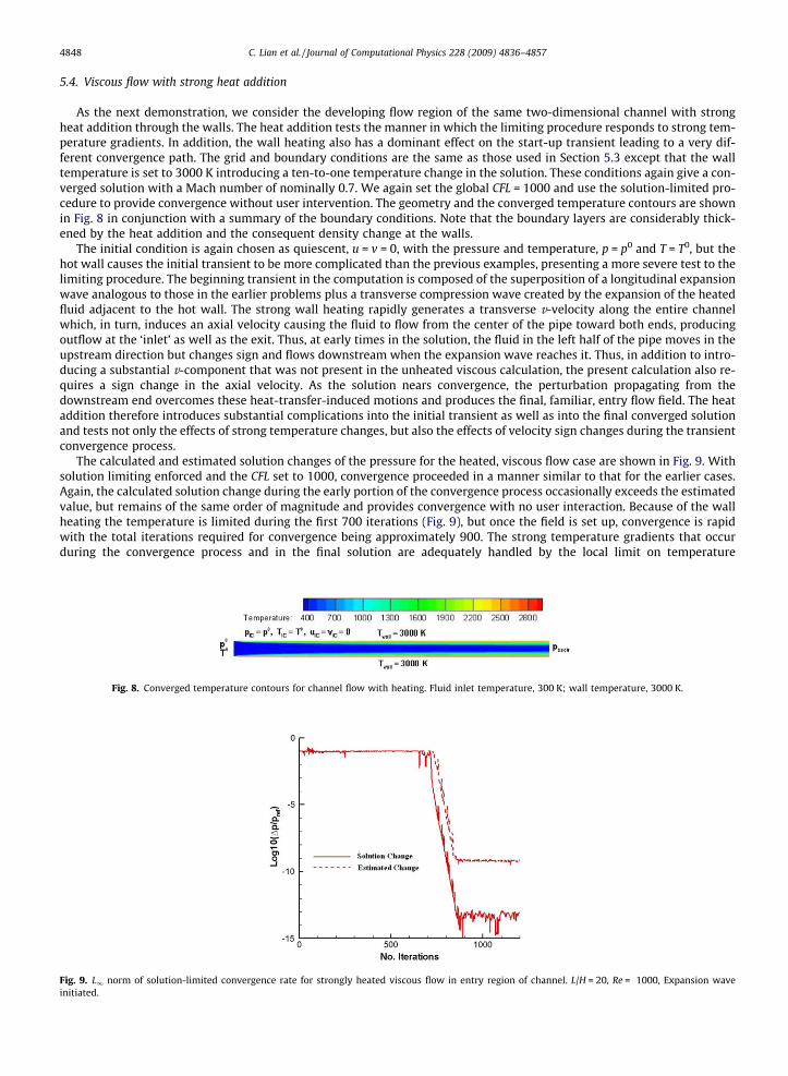
As the next demonstration, we consider the developing flow region of the same two-dimensional channel with strongheat addition through the walls. The heat addition tests the manner in which the limiting procedure responds to strong tem-perature gradients. In addition, the wall heating also has a dominant effect on the start-up transient leading to a very dif-ferent convergence path. The grid and boundary conditions are the same as those used in Section 5.3 except that the walltemperature is set to 3000 K introducing a ten-to-one temperature change in the solution. These conditions again give a con-verged solution with a Mach number of nominally 0.7. We again set the global CFL = 1000 and use the solution-limited pro-cedure to provide convergence without user intervention. The geometry and the converged temperature contours are shownin Fig. 8 in conjunction with a summary of the boundary conditions. Note that the boundary layers are considerably thick-ened by the heat addition and the consequent density change at the walls.

The initial condition is again chosen as quiescent, u = v = 0, with the pressure and temperature, p = p0 and T = T0, but thehot wall causes the initial transient to be more complicated than the previous examples, presenting a more severe test to thelimiting procedure. The beginning transient in the computation is composed of the superposition of a longitudinal expansionwave analogous to those in the earlier problems plus a transverse compression wave created by the expansion of the heatedfluid adjacent to the hot wall. The strong wall heating rapidly generates a transverse v-velocity along the entire channelwhich, in turn, induces an axial velocity causing the fluid to flow from the center of the pipe toward both ends, producingoutflow at the ‘inlet’ as well as the exit. Thus, at early times in the solution, the fluid in the left half of the pipe moves in theupstream direction but changes sign and flows downstream when the expansion wave reaches it. Thus, in addition to intro-ducing a substantial v-component that was not present in the unheated viscous calculation, the present calculation also re-quires a sign change in the axial velocity. As the solution nears convergence, the perturbation propagating from thedownstream end overcomes these heat-transfer-induced motions and produces the final, familiar, entry flow field. The heataddition therefore introduces substantial complications into the initial transient as well as into the final converged solutionand tests not only the effects of strong temperature changes, but also the effects of velocity sign changes during the transientconvergence process.

The calculated and estimated solution changes of the pressure for the heated, viscous flow case are shown in Fig. 9. Withsolution limiting enforced and the CFL set to 1000, convergence proceeded in a manner similar to that for the earlier cases.Again, the calculated solution change during the early portion of the convergence process occasionally exceeds the estimatedvalue, but remains of the same order of magnitude and provides convergence with no user interaction. Because of the wallheating the temperature is limited during the first 700 iterations (Fig. 9), but once the field is set up, convergence is rapidwith the total iterations required for convergence being approximately 900. The strong temperature gradients that occurduring the convergence process and in the final solution are adequately handled by the local limit on temperature

Fig. 8. Converged temperature contours for channel flow with heating. Fluid inlet temperature, 300 K; wall temperature, 3000 K.

Fig. 9. L1 norm of solution-limited convergence rate for strongly heated viscous flow in entry region of channel. L/H = 20, Re = 1000, Expansion waveinitiated.


(a = 0.1) and did not require redefinition of the reference temperature. In addition, the initial backward flow in the upstreamhalf of the tube and the subsequent reversal were handled by the velocity change limit.

Some details of the convergence process are given in Figs. 10 and 11 to support the convergence plots in Fig. 9. Fig. 10shows the CFL distribution for the first step of the iteration. The expansion wave at the downstream end causes the time stepat the outlet plane of cells to be limited. The wall thermal condition imposes a limit at the wall boundary cells from the verybeginning, which is not so clearly shown in the contours plot because of the refined grid near the wall but is shown by themore detailed plots of the CFL profiles on the top left of Fig. 10.

Fig. 11 shows a sequence of axial velocity contour plots throughout the convergence process. At time steps one and two,the velocity profile is seen developing near both ends with larger values in the middle of the channel than along the walls

Fig. 10. CFL distributions for the first step of the iteration. Top: CFL profiles at two different locations. Bottom: CFL contours in the channel.

Fig. 11. Axial velocity contour plots showing solution during convergence. For clarity, the color scheme for the contour plots has been changed for differentiteration steps. Plots not having a color legend follow the legend above them.


because of the smaller time steps on the walls. Note that from 50 to 600 time steps that there are large regions with sub-stantial negative axial velocity components. As the solution approaches convergence (800 steps), the velocity field becomespositive throughout with the solution eventually reaching the familiar pattern for an entry duct.

5.5. Viscous flow in a converging–diverging nozzle

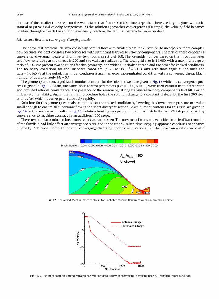
The above test problems all involved nearly parallel flow with small streamline curvature. To incorporate more complexflow features, we next consider two test cases with significant transverse velocity components. The first of these concerns aconverging–diverging nozzle with an inlet-to-throat area ratio of 100. The Reynolds number based on the throat diameterand flow conditions at the throat is 200 and the walls are adiabatic. The total grid size is 14,000 with a maximum aspectratio of 200. We present two solutions for this geometry, one with an unchoked throat, and the other for choked conditions.The boundary conditions for the unchoked cased are: p0 = 1.4e5 Pa, T0 = 300 K and zero flow angle at the inlet andpback = 1.01e5 Pa at the outlet. The initial condition is again an expansion-initiated condition with a converged throat Machnumber of approximately Ma = 0.7.

The geometry and converged Mach number contours for the subsonic case are given in Fig. 12 while the convergence pro-cess is given in Fig. 13. Again, the same input control parameters (CFL = 1000, a = 0.1) were used without user interventionand provided reliable convergence. The presence of the reasonably strong transverse velocity components had little or noinfluence on reliability. Again, the limiting procedure holds the solution change to a constant plateau for the first 200 iter-ations after which it converged reasonably rapidly.

Solutions for this geometry were also computed for the choked condition by lowering the downstream pressure to a valuesmall enough to ensure all supersonic flow in the short divergent section. Mach number contours for this case are given inFig. 14, with convergence results in Fig. 15. Solution limiting was present for approximately the first 200 steps followed byconvergence to machine accuracy in an additional 600 steps.

These results also produce robust convergence as can be seen. The presence of transonic velocities in a significant portionof the flowfield had little effect on convergence rates, and the solution-limited time stepping approach continues to enhancereliability. Additional computations for converging–diverging nozzles with various inlet-to-throat area ratios were also

Fig. 12. Converged Mach number contours for unchoked viscous flow in converging–diverging nozzle.

Fig. 13. L1 norm of solution-limited convergence rate for viscous flow in converging–diverging nozzle. Unchoked throat condition.

Fig. 15. L1 norm of solution-limited convergence rate for viscous flow in converging–diverging nozzle. Choked throat condition.

Fig. 14. Converged Mach number contours for choked viscous flow in converging–diverging nozzle.


conducted for both choked and unchoked conditions. In all cases, the solution-limited time stepping method provided effec-tive convergence with no change in user-specified conditions.

5.6. Flow past a backward-facing step

The next example concerns the flow over a backward-facing step. The backward facing step problem is significant for thesolution-limited time stepping procedure in that the flow must change sign during the convergence process and both veloc-ity components have regions of positive and negative signs in the converged solution. The results verify that the velocity lim-iting procedure does not adversely affect convergence when velocity sign changes are a characteristic of the convergedflowfield. Two different step heights were considered as shown in Fig. 16. The first [35] has a step height to inlet height ratioof 1:9 while the second has a ratio of 1:2 corresponding to the experimental configuration of Armaly et al. [36]. Both casesare compression wave initiated with specified upstream Mach numbers (0.128 and 0.004) and the same upstream temper-ature (300 K) and the same back pressure (1.01e5 Pa). The Reynolds numbers based on step height are 370 and 50. The gridsizes are 17,000 and 23,000 with maximum cell aspect ratio of 300. The convergences for the two cases are similar and onlythat for the second case is shown in Fig. 17. The convergence rate decreases after around 500 iterations because of the recir-culation zone at the backward facing step. The time stepping method is operational only during approximately the first 200iterations. The results clearly show that the limiting procedure remains effective in flow fields characterized by sign changesin both velocity components.

5.7. Transonic flow over an RAE 2822 airfoil

The above problems consider relatively simple problems that test various characteristics of the solution-limited timestepping method. To illustrate the method in more practical applications, we include two additional cases in the next twosections.

The first of these concerns transonic flow over an RAE 2822 airfoil. A grid of 24,000 cells is used. The free stream Machnumber is 0.729 while the static pressure and temperature are 1.0e5 Pa and 273 K, respectively. The solution shown is for an

Fig. 16. Schematic of backward-facing step and converged velocity contours. Top: 1:9 step height ratio; Bottom: 1:2 exit height ratio.

Fig. 17. L1 norm of solution-limited convergence rate for backward-facing step flow. CFL = 1000, a = 0.1.


angle of attack of 2.31�. These conditions correspond to a Reynolds number of 6.5 million based on a chord length of 1.0 ft. Acontour plot of the Mach number near the airfoil is shown in Fig. 18. The pressure coefficient on the airfoil (Cp) is comparedexperimental measurements in Fig. 19.

The turbulence characteristics were simulated by the k–x turbulence model [37]. To apply the limiting procedure, wechoose normalization values for k and x according to the procedure described in Section 3.3. For the turbulent kinetic en-ergy, we choose a reference value kref ¼ 3

2 ðI � Uref Þ2 where I is the turbulence intensity. The turbulence dissipation rate x has a

Fig. 18. Mach number contours near airfoil region.

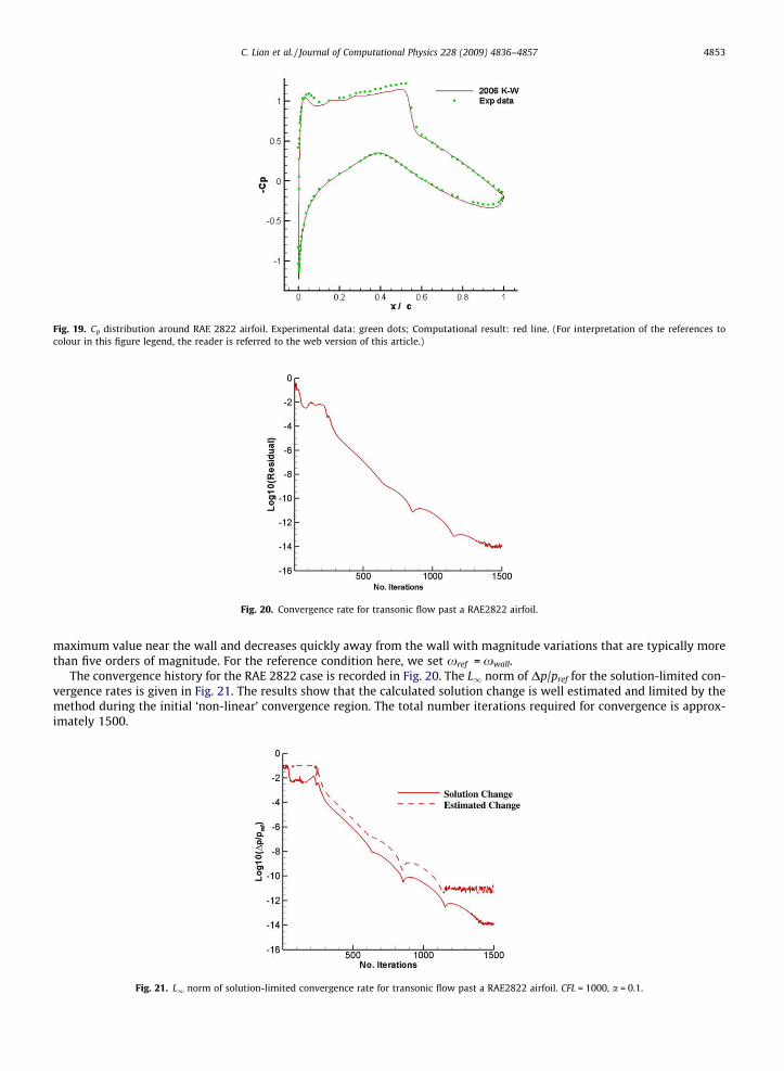
Fig. 19. Cp distribution around RAE 2822 airfoil. Experimental data: green dots; Computational result: red line. (For interpretation of the references tocolour in this figure legend, the reader is referred to the web version of this article.)

Fig. 20. Convergence rate for transonic flow past a RAE2822 airfoil.


maximum value near the wall and decreases quickly away from the wall with magnitude variations that are typically morethan five orders of magnitude. For the reference condition here, we set xref = xwall.

The convergence history for the RAE 2822 case is recorded in Fig. 20. The L1 norm of Dp/pref for the solution-limited con-vergence rates is given in Fig. 21. The results show that the calculated solution change is well estimated and limited by themethod during the initial ‘non-linear’ convergence region. The total number iterations required for convergence is approx-imately 1500.

Fig. 21. L1 norm of solution-limited convergence rate for transonic flow past a RAE2822 airfoil. CFL = 1000, a = 0.1.


5.8. Mixing and combustion of hydrogen (H2) and oxygen (O2) in rocket engine combustor

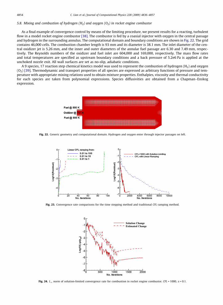
As a final example of convergence control by means of the limiting procedure, we present results for a reacting, turbulentflow in a model rocket engine combustor [38]. The combustor is fed by a coaxial injector with oxygen in the central passageand hydrogen in the surrounding annulus. The computational domain and boundary conditions are shown in Fig. 22. The gridcontains 46,000 cells. The combustion chamber length is 93 mm and its diameter is 38.1 mm. The inlet diameter of the cen-tral oxidizer jet is 5.26 mm, and the inner and outer diameters of the annular fuel passage are 6.30 and 7.49 mm, respec-tively. The Reynolds numbers of the oxidizer and fuel inlet are 604,000 and 169,000, respectively. The mass flow ratesand total temperatures are specified as upstream boundary conditions and a back pressure of 5.2e6 Pa is applied at theunchoked nozzle exit. All wall surfaces are set as no-slip, adiabatic conditions.

A 9 species, 17 reaction step chemical kinetics model was used to represent the combustion of hydrogen (H2) and oxygen(O2) [39]. Thermodynamic and transport properties of all species are expressed as arbitrary functions of pressure and tem-perature with appropriate mixing relations used to obtain mixture properties. Enthalpies, viscosity and thermal conductivityfor each species are taken from polynomial expressions. Species diffusivities are obtained from a Chapman–Enskogexpression.

Fig. 22. Generic geometry and computational domain. Hydrogen and oxygen enter through injector passages on left.

Fig. 23. Convergence rate comparisons for the time stepping method and traditional CFL ramping method.

Fig. 24. L1 norm of solution-limited convergence rate for combustion in rocket engine combustor. CFL = 1000, a = 0.1.

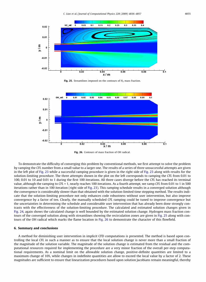
Fig. 25. Streamlines imposed on the contours of H2 mass fraction.

Fig. 26. Contours of mass fraction of OH radical.


To demonstrate the difficulty of converging this problem by conventional methods, we first attempt to solve the problemby ramping the CFL number from a small value to a larger one. The results of a series of three unsuccessful attempts are givenin the left plot of Fig. 23 while a successful ramping procedure is given in the right side of Fig. 23 along with results for thesolution-limiting procedure. The three attempts shown in the plot on the left corresponds to ramping the CFL from 0.01 to100, 0.01 to 10 and 0.01 to 1 during the first 100 iterations. All three cases diverge before the CFL has reached its terminalvalue, although the ramping to CFL = 1, nearly reaches 100 iterations. As a fourth attempt, we ramp CFL from 0.01 to 1 in 500iterations rather than in 100 iteration (right side of Fig. 23). This ramping schedule results in a converged solution althoughthe convergence is considerably slower than that obtained with the solution-limited time stepping method. The results indi-cate that the solution-limiting procedure not only enhances code robustness without user intervention, but also improveconvergence by a factor of ten. Clearly, the manually scheduled CFL ramping could be tuned to improve convergence butthe uncertainties in determining the schedule and considerable user intervention that has already been done strongly con-trasts with the effectiveness of the solution-limiting procedure. The calculated and estimated solution changes given inFig. 24, again shows the calculated change is well bounded by the estimated solution change. Hydrogen mass fraction con-tours of the converged solution along with streamlines showing the recirculation zones are given in Fig. 25 along with con-tours of the OH radical which marks the flame location in Fig. 26 to demonstrate the character of this flowfield.

6. Summary and conclusions

A method for diminishing user intervention in implicit CFD computations is presented. The method is based upon con-trolling the local CFL in such a manner as to ensure that the local solution change is never more than a small fraction ofthe magnitude of the solution variable. The magnitude of the solution change is estimated from the residual and the com-putational resources required for implementing the procedure are a very minor fraction of the overall per-step computa-tional requirements. As a nominal limit on the allowable solution change, positive-definite quantities are limited to amaximum change of 10%, while changes in indefinite quantities are allow to exceed the local value by a factor of 2. Thesemagnitudes are sufficient to ensure that linearization procedures based upon solution Jacobians remain meaningful, thereby


precluding solution migrations to unphysical regions, yet large enough to allow rapid solution convergence. In addition thesolution-change limit ensures that quantities such as pressure, density and temperature cannot become negative, again pre-venting a common difficulty in CFD solutions. Other limiting magnitudes have been tried, but the 10% limit appears to be areasonable compromise between overly conservative changes that slow convergence unacceptably and more aggressivechanges that may fail to keep the solution within reasonable bounds over the complete computation.

Perhaps the most important element for success of the method is determining acceptable reference conditions uponwhich to base the solution change. Our experience indicates that while all variables must be limited, the most critical param-eter is the pressure. The characteristic pressure in a given problem or a series of different problems may be related to thelocal dynamic pressure, the local shear stress, the local flow acceleration or the local body force terms. Proper balancingof these with the pressure gradient is important for controlling the allowable change in pressure. Velocity, likewise, mustbe limited, but in such a manner that the velocity may change sign, whereas temperature limitation based simply uponthe thermodynamic temperature appears sufficient in the conditions computed to date.

As a demonstration of the method, more than a half-dozen different problems, each with an added degree of difficulty, arepresented. All solutions started from a quiescent initial condition with either an expansion fan from the exit boundary or ashock from the inlet boundary. For all cases, a single, user-specified CFL = 1000 was used and in all cases, the solution con-verged reliably and efficiently without user intervention or changes in the control parameters apart from those variationsdetermined by the limiting procedure itself. The specific cases and variables tested along with their relevance include:

� One-dimensional flow: verifies ability to scale the solution change for conditions in which the velocity is zero in all cellsand the pressure is constant everywhere except for one cell;

� Two-dimensional inviscid flow: verifies that findings from one-dimensional solutions are applicable in multi-dimensions;� Two-dimensional viscous flow: incorporates effects of boundary layers and shear stress in solution change limits and ref-

erence conditions;� Viscous flow with strong heating: adds considerable complexity to the starting transient, including directional changes in

the velocity, while also incorporating the effects of strong temperature gradients and tests the effects of solution limits fortemperature;

� Nozzle flows: tests the capability of the solution-limiting method in the presence of flows with large changes in the flowangle for both choked and unchoked conditions;

� Flow over a backward-facing step: incorporates the effect of recirculation, reverse flow and sign changes in the velocity;� Transonic flow over RAE 2822 airfoil: incorporates turbulent flow at high Reynolds number flow along with shocks;� Mixing and combustion of hydrogen and oxygen: tests the capability of the solution-limited time stepping method for

multi-species and reacting flow in a complicated flow field.

In addition to the cases represented here, the method has also been tried for a large number of other problems. Our expe-rience has been that the method greatly decreases the number of unsuccessful runs and nearly eliminates the need for userintervention in a wide variety of problems. Overall, the solution-limited time stepping procedure automatically adjusts theCFL number for each grid according to the estimated solution change and greatly reduces the sensitivity to initial conditionsfor various types of flows. The method requires negligible additional computing time and is easily implemented into anyimplicit CFD code.

References

[1] R.H. Bush, G.D. Power, C.E. Towne, WIND: the production flow solver of the NPARC alliance, in: 36th AIAA Aerospace Sciences Meeting and Exhibit,Reno, NV, January 12–January 15, 1998, AIAA Paper 1998-0935.

[2] N.T. Frink, S.Z. Pirzadeh, P.C. Parikh, M.J. Pandya, M.K. Bhat, The NASA tetrahedral unstructured software system (TetrUSS), in: 22nd InternationalCongress of Aeronautical Sciences, Harrogate, United Kingdom, August 27–September 1, 2000, ICAS Paper No. 0241.

[3] V. Sankaran, C.L. Merkle, X. Zeng, D. Li, Influence of large-scale pressure changes on preconditioned solutions at low speeds, AIAA J. 42 (12) (2004)2490–2498.

[4] W. Mulder, B. van Leer, Experiments with implicit upwind methods for the Euler equations, J. Comput. Phys. 59 (1985) 232–246.[5] E. Issman, G. Degrez, H. Deconinck, Implicit upwind residual-distribution Euler and Navier–Stokes solver on unstructured meshes, AIAA J. 34 (10)

(1996) 2021–2028.[6] D. Vanderstraeten, A. Csk, D. Rose, An expert-system to control the CFL number of implicit upwind methods, Technical Report TM 304, Universiteit

Leuven, March 2000.[7] H.M. Bücker, B. Pollul, A. Rasch, On CFL evolution strategies for implicit upwind methods in linearized Euler equations, Technical Report, RWTH Aachen

University, August 7, 2006.[8] E.A. Luke, X.-L. Tong, J. Wu, L. Tang, P. Cinnella, A step towards ‘Shape-Shifting’ algorithms: reactive flow simulations using generalized grids, AIAA

Paper No. 2001-0897, 2001.[9] C. Merkle, D. Li, V. Sankaran, Multi-disciplinary computational analysis in propulsion, AIAA Paper No. 2006-4575, 2001.

[10] H. Nessyahu, E. Tadmor, Non-oscillatory central differencing for hyperbolic conservation laws, J. Comput. Phys. 87 (1990) 408–463.[11] G. Jiang, E. Tadmor, Non-oscillatory central schemes for multidimensional hyperbolic conservation laws, SIAM J. Sci. Comput. 19 (1998) 1892–1917.[12] P.D. Lax, Weak solutions of nonlinear hyperbolic equation and their numerical computation, Commun. Pure Appl. Math. 7 (1954) 159–193.[13] B. van Leer, Flux-vector splitting for the Euler equation, NASA Langley Research Center Hampton, ICASE Report 82-30, 1982.[14] T. Linde, A practical, general-purpose Riemann solver for hyperbolic conservation laws, in: Seventh International Conference on Numerical Methods in

Fluid Dynamics, Clarendon, 2001.[15] M.-S. Liou, C. Steffen, A new flux splitting scheme, J. Comput. Phys. 109 (1993) 23–93.[16] M.-S. Liou, J. Edwards, Low-diffusion flux splitting methods for flows at all speed, AIAA J. 36 (9) (1998) 1610–1617.


[17] P. Roe, Approximate Riemann solvers, parameter vectors and difference schemes, J. Comput. Phys. 43 (1981) 357–372.[18] S. Godunov, A finite-difference method for the numerical computation and discontinuous solutions of the equations of fluid dynamics, Mat. Sb. 47

(1959) 271–306.[19] S. Osher, F. Solomon, Upwind schemes for hyperbolic systems of conservation laws, Math. Comput. 38 (1982) 339–374.[20] E. Turkel, Preconditioning methods for solving the incompressible and low speed compressible equations, J. Comput. Phys. 72 (1987) 277–298.[21] B. van Leer, W. Lee, P. Roe, Characteristic time-stepping or local preconditioning of the euler equations, AIAA 1991-1552-CP, Computational Fluid

Dynamics Conference, Honolulu, 1991.[22] H. Viviand, Pseudo-unsteady systems for steady inviscid flow calculation, in: F. Angrand et al. (Eds.), Numerical Methods for the Euler Equations of

Fluid Dynamics, SIAM, Philadelphia, 1985.[23] W. Briley, H. McDonald, S. Shamroth, A low Mach number Euler formulation and application to time iterative LBI schemes, AIAA J. 21 (10) (1983) 1467–

1469.[24] Y. Choi, C. Merkle, The application of preconditioning to viscous flows, J. Comput. Phys. 105 (1993) 207–223.[25] W. Briley, H. McDonald, On the structure and use of linearized block implicit schemes, J. Comput. Phys. 34 (1980) 54–73.[26] W. Briley, H. McDonald, An overview and generalization of implicit Navier–Stokes algorithms and approximate factorization, Comput. Fluids 30 (2001)

807–828.[27] J. Thomas, R. Walters, Upwind relaxation algorithm for the Navier–Stokes equations, AIAA J. 25 (4) (1987) 527–534.[28] K. Vanden, D. Whitfield, Direct and iterative algorithms for the three-dimensional euler equations, AIAA 1993-3378-CP, 1993.[29] Joo Sung Kim, Oh Joon Kwon, An efficient and robust implicit operator for upwind point Gauss–Seidel method, J. Comput. Phys. 224 (2007) 1124–1144.[30] C. Lombard, J. Bardina, E. Venkatapathy, J. Oliger, Multi-dimensional formulation of CSCM – an upwind flux difference eigenvector split method for the

compressible Navier–Stokes equations, AIAA Paper No. 1983-1895, 1983.[31] R. MacCormack, G. Candler, The solution of the Navier–Stokes equations using Gauss–Seidel line relaxation, Comput. Fluids 17 (1989) 135–150.[32] Y. Saad, M. Schultz, GMRES: a generalized minimal residual algorithm for solving nonsymmetric linear system, SIAM J. Sci. Stat. Comput 7 (3) (1986)

856–869.[33] H. Guillard, C. Viozat, On the behaviour of upwind schemes in the low Mach number limit, Comput. Fluids 28 (1) (1999) 63–86.[34] Durst Franz, An Introduction to the Theory of Fluid Flows, 2008, ISBN:9783540713425.[35] D. Driver, H. Seegmiller, Features of a reattaching turbulent shear layer in divergent channel flow, AIAA J. 23 (2) (1985) 163–171.[36] B.F. Armaly, F. Durst, J.C.F. Pereira, B. Schonung, Experimental and theoretical investigation of backward-facing step flow, J. Fluid Mech. 127 (1983)

473–496.[37] D. Wilcox, Turbulence Modeling for CFD, second ed., DCW Industries, La Canada, CA, 1998.[38] P. Tucker, S. Menon, C. Merkle, J. Oefelein, V. Yang, An approach to improved credibility of CFD simulations for rocket injector design, in: 43rd AIAA/

ASME/SAE/ASEE Joint Propulsion Conference and Exhibit, July 8–July 11, Cincinnati, OH, 2007.[39] M. Ó Conaire, H.J. Curran, J.M. Simmie, W.J. Pitz, C.K. Westbrook, A comprehensive modeling study of hydrogen oxidation, Int. J. Chem. Kinet. 36 (2004)

603–622.

Solution-limited time stepping to enhance reliability in CFD ...

Documents

Transcript of Solution-limited time stepping to enhance reliability in CFD ...