CFD modelling of Heat Exchanger Fouling - UNSWorks

CFD modelling of

Heat Exchanger Fouling

A Thesis submitted in fulfillment of the requirements for the degree of

Doctor of Philosophy [PhD]

29th July 2005

By Patrick Walker

Department of Chemical Engineering and Industrial Chemistry

University of New South Wales

Sydney

Australia

2

Abstract Heat exchanger fouling is the deposition of material onto the heat transfer surface causing a

reduction in thermal efficiency. A study using Computational Fluid Dynamics (CFD) was

conducted to increase understanding of key aspects of fouling in desalination processes.

Fouling is a complex phenomenon and therefore this numerical model was developed in

stages. Each stage required a critical assessment of each fouling process in order to design

physical models to describe the process’s intricate kinetic and thermodynamic behaviour.

The completed physical models were incorporated into the simulations through employing

extra transport equations, and coding additional subroutines depicting the behaviour of the

aqueous phase involved in the fouling phenomena prominent in crystalline streams.

The research objectives of creating a CFD model to predict fouling behaviour and assess

the influence of key operating parameters were achieved. The completed model of the key

crystallisation fouling processes monitors the temporal variation of the fouling resistance.

The fouling rates predicted from these results revealed that the numerical model

satisfactorily reproduced the phenomenon observed experimentally. Inspection of the CFD

results at a local level indicated that the interface temperature was the most influential

operating parameter. The research also examined the likelihood that the crystallisation and

particulate fouling mechanisms coexist. It was found that the distribution of velocity

increased the likelihood of the particulate phase forming within the boundary layer, thus

emphasizing the importance of differentiating between behaviour within the bulk and the

boundary layer. These numerical results also implied that the probability of this composite

fouling was greater in turbulent flow. Finally, supersaturation was confirmed as the key

parameter when precipitation occurred within the bulk/boundary layer.

This investigation demonstrated the advantages of using CFD to assess heat exchanger

fouling. It produced additional physical models which when incorporated into the CFD

code adequately modeled key aspects of the crystallisation and particulate fouling

mechanisms. These innovative modelling ideas should encourage extensive use of CFD in

future fouling investigations. It is recommended that further work include detailed

3

experimental data to assist in defining the key kinetic and thermodynamic parameters to

extend the scope of the required physical models.

4

Table of Contents

Abstract .................................................................................................................................. 2

Acknowledgments................................................................................................................ 10

Nomenclature ....................................................................................................................... 12

1. Introduction .............................................................................................................. 19

2. Literature Review..................................................................................................... 22

2.1. Introduction.......................................................................................................... 22

2.2. Heat Exchanger Fouling....................................................................................... 23

2.2.1. Definition ..................................................................................................... 23

2.2.2. A basic description of fouling ...................................................................... 23

2.2.3. The Consequences of Fouling...................................................................... 25

2.2.4. The Purpose of this Study ............................................................................ 27

2.3. Influential Aspects of Fouling.............................................................................. 27

2.3.1. Fouling Mechanisms .................................................................................... 28

2.3.2. Fouling Processes......................................................................................... 29

2.3.3. Influential Parameters .................................................................................. 32

2.3.4. Composite Fouling ....................................................................................... 35

2.4. Models Describing Fouling.................................................................................. 36

2.4.1. Fouling Curves: an overall view .................................................................. 36

2.4.2. Modelling the processes and mechanisms ................................................... 38

2.4.2.1. The Induction Period............................................................................ 38

2.4.2.2. The Roughness Delay Period ............................................................... 41

2.4.2.3. Deposition: Resistance ......................................................................... 43

2.4.2.4. Deposition: the Lagrangian modelling approach ................................. 48

2.4.2.5. Deposition: the Eulerian modelling approach...................................... 51

2.4.2.6. Deposition: Composite Fouling ........................................................... 54

2.4.2.7. Removal ............................................................................................... 55

2.5. Techniques for the analysis of Fouling ................................................................ 56

5

2.5.1. Key Experimental Investigations ................................................................. 56

2.5.2. Using CFD to Investigate fouling ................................................................ 57

2.5.3. Advantages of Using CFD over Experimental Techniques ......................... 58

2.6. Closing Statement ................................................................................................ 59

3. Materials................................................................................................................... 60

3.1. Computational Fluid Dynamics – An introduction.............................................. 60

3.2. The Strategy for Validation of the fouling model................................................ 61

3.2.1. Transport Phenomena: Empirical Correlations............................................ 62

3.2.2. Fouling Processes: The Experimental Data ................................................. 68

4. Methodology ............................................................................................................ 71

4.1. CFD: The Governing Equations .......................................................................... 71

4.1.1. The Transport Equation................................................................................ 71

4.1.2. The Turbulence models................................................................................ 72

4.1.2.1. The Standard k-ε model ....................................................................... 73

4.1.2.2. The Low Reynolds number k-ε model................................................. 77

4.1.3. Verification Strategy .................................................................................... 79

4.2. The Energy Transport Equation ........................................................................... 80

4.3. The Crystallisation Mechanism - Eulerian Modelling Approach ........................ 80

4.3.1. The Eulerian Modelling Approach to the homogeneous phase ................... 80

4.3.2. Precipitation in bulk/boundary layer............................................................ 82

4.3.3. Crystallisation Fouling: Precipitation at the surface .................................... 83

4.4. The Particulate Mechanism Lagrangian Modelling Approach ............................ 85

4.4.1. The Lagrangian Modelling Approach to the discrete particulate phase ...... 85

4.4.2. Particulate Generation: Precipitation within bulk/boundary layer............... 85

4.4.3. Particulate deposition: Additional Forces acting on Particle ....................... 86

4.4.4. Particulate Flux: Quantifying the deposition of the Particulate Material .... 88

4.4.5. Composite Fouling: The Combined CFD model ......................................... 89

4.4.6. Assumptions used in the Lagrangian Modelling Approach......................... 90

4.5. The transient nature of foulant deposition ........................................................... 91

6

4.5.1. The Moving Boundary Approach ................................................................ 91

4.5.2. The Distribution of Heat Flux ...................................................................... 92

4.5.3. The Nucleation Relationship........................................................................ 93

4.5.4. The Crystallisation Mechanism - Moving Boundary Technique................. 95

4.5.5. Calculating the Fouling Resistance Using CFX-4.3 .................................... 98

4.5.6. The Combined Code depicting the Moving Boundary Technique: The

developed CFX-4.3 FORTRAN Codes ..................................................................... 100

4.6. The Inclusion of Roughness using CFX-5.7 ...................................................... 101

4.6.1. The Roughness Algorithm ......................................................................... 102

4.6.2. The Lower and Upper Limit of Roughness ............................................... 103

4.6.3. The Roughness Relationship...................................................................... 104

4.6.4. Methodology Calculating the Fouling Resistance ..................................... 106

4.6.5. The Moving Boundary-Roughness Code developed in CFX-5.7 .............. 107

5. Development of 2D model with CaSO4 Precipitation occurring within flow using an

Eulerian modelling approach ............................................................................................. 113

5.1. Introduction........................................................................................................ 113

5.2. Model Boundary Conditions .............................................................................. 113

5.3. Verification of the Precipitation Model ............................................................. 115

5.4. Examination of Calcium Sulphate Precipitation within different flow regimes and

under various conditions ................................................................................................ 119

5.4.1. Precipitation in Laminar Flow ................................................................... 120

5.4.1.1. Observation of Generation ................................................................. 120

5.4.1.2. Effect of Velocity in Laminar Flow................................................... 122

5.4.1.3. Effect of Velocity at Varying Inlet Supersaturation .......................... 126

5.4.1.4. Effect of Velocity at Various System Temperatures.......................... 127

5.4.2. Precipitation in Fully Turbulent Flow........................................................ 128

5.4.2.1. Verification for the Turbulent Conditions.......................................... 128

5.4.2.2. Isothermal Fully Turbulent Flow ....................................................... 129

5.4.2.3. The Effect of Temperature Gradients in Fully Turbulent Flow......... 131

5.5. Validation: Modelling a Particulate Phase......................................................... 134

5.6. Summary: Usefulness of CFD ........................................................................... 136

7

6. Study of CaSO4 Precipitation in Laminar Flows in pipes and slits under Isothermal

Conditions .......................................................................................................................... 138

6.1. Introduction........................................................................................................ 138


6.3. Examination of Precipitation Behavior within different Geometries ................ 139

6.3.1. Effect of Residence Time and Velocity ..................................................... 139

6.3.2. Precipitation in different Geometries ......................................................... 141

6.3.2.1. Equal Shear Stress.............................................................................. 141

6.3.2.2. Equal Velocity.................................................................................... 143

6.3.2.3. Equal Reynolds Number .................................................................... 145

6.4. Summary ............................................................................................................ 147

7. Development of a steady state 2D model of fouling mechanisms to focus on

deposition. .......................................................................................................................... 148

7.1. Introduction........................................................................................................ 148


7.3. Results and Discussions ..................................................................................... 150

7.3.1. Model development.................................................................................... 150

7.3.1.1. Turbulent Models: Developing Flow................................................. 151

7.3.1.2. The Operation of the Lagrangian Model............................................ 153

7.3.2. Key Results and Validation........................................................................ 158

7.3.2.1. Crystallisation Fouling Mechanism: Re ≈ 4000, Tin = 323 K............ 158

7.3.2.2. Crystallisation Fouling Mechanism: Re ≈ 5000, Tin = 343 K............ 159

7.3.2.3. Combined Crystallisation and Particulate Fouling Mechanism: Re ≈

5000, Tin = 343 K ................................................................................................... 161

7.3.2.4. Relative Effect of Supersaturation and Temperature: Re ≈ 5000, Tin =

343 K ............................................................................................................ 162

7.3.2.5. Assessing the Precipitation through examining the calcium ion profiles:

Re ≈ 5000, Tin = 343 K........................................................................................... 164

7.3.2.6. Combined Crystallisation and Particulate Fouling Mechanism: Re ≈

4000, Tin = 323 K ................................................................................................... 166

8

7.3.3. Physical Method: Relating Issues .............................................................. 167

7.3.3.1. The Kinetics of Precipitation ............................................................. 168

7.3.3.2. Solution Thermodynamics ~ The Solubility ...................................... 172

7.3.3.3. Steady State v. Transient.................................................................... 173

8. Development and Validation of an Unsteady State Numerical Model of the

Crystallisation Fouling Mechanism within a Crystalline System...................................... 175

8.1. Introduction........................................................................................................ 175


8.3. Model Verification ............................................................................................. 177

8.3.1. Grid Analysis ............................................................................................. 177

8.3.2. Selection of the Heat Flux Method ............................................................ 178

8.4. Results and Discussion....................................................................................... 180

8.4.1. Using the Nucleation Relationship ............................................................ 181

8.4.2. Numerical Fouling ..................................................................................... 183

8.4.2.1. Operating Parameters ......................................................................... 183

8.4.2.2. Fouling Resistance ............................................................................. 188

8.4.3. Validation of Numerical Results................................................................ 190

9. Derivation and Validation of a Numerical Expression Describing the Influence of

Surface Roughness on Crystallisation Fouling .................................................................. 194

9.1. Introduction........................................................................................................ 194

9.2. Roughness Model Boundary Conditions ........................................................... 195

9.3. Model Verification ............................................................................................. 195

9.4. Results and Discussion....................................................................................... 196

9.4.1. Difference in turbulent models................................................................... 197

9.4.2. Operation of the Roughness Model ........................................................... 200

9.4.3. Use of the Roughness Relationship in the Numerical Fouling Model....... 206

9.4.3.1. The Operating Parameters.................................................................. 206

9.4.3.2. The Fouling Resistances .................................................................... 212

9.4.4. Validation of The Numerical Results......................................................... 214

9.5. Enhancement of the Roughness Model.............................................................. 218

10. Conclusions and Recommendations ...................................................................... 221

9

10.1. Conclusions .................................................................................................... 221

10.2. Recommendations.......................................................................................... 227

References .......................................................................................................................... 230

Appendix A. Papers Produced from this Thesis ................................................... 237

Appendix B. The Simulation Command Files...................................................... 238

B.1 The CFX 4.3 Command Language written for CaSO4 Precipitation in Laminar

Flows in an Annular Geometry ...................................................................................... 238

B.2 The CFX 4.3 Command Language written for CaSO4 Precipitation in turbulent

Flows in an Annular Geometry ...................................................................................... 240

B.3 CFX 4.3 Command Language written for Combined Precipitation, Particulate

fouling and Crystallisation fouling ................................................................................ 242

B.4 The CFX 4.3 Command Language written for the fouling simulations in this

research .......................................................................................................................... 244

B.5 The CFX 5.7 command Language written for the fouling simulations in this

research .......................................................................................................................... 247

Appendix C. The Simulation User-Subroutines ...................................................... 254

C.1 The FORTRAN Codes developed in CFX-4.3 to model CaSO4 Precipitation in

Laminar and turbulent Flows in an Annular Geometry ................................................. 254

C.2 The FORTRAN Codes developed in CFX-4.3 to model CaSO4 Precipitation and

the subsequent transport of particles as a solid phase using a Lagrangian transport

equation .......................................................................................................................... 255

C.3 The FORTRAN Codes developed in CFX-4.3 to model Heat Exchanger Fouling .

............................................................................................................................ 258

C.4 The FORTRAN Codes developed in CFX-5.7 to model Heat Exchanger Fouling .

............................................................................................................................ 261

10

Acknowledgments

I’d like to thank my supervisors Roya Shiehkholeslami and Soji Adesina. Special thanks

goes to Farid Fahiminia and Teresa Chong for sharing their experimental results with me. I

would also like to thank Mike Brungs, the School of Chemical Engineering, Tim Hesketh

and the Faculty of Engineering for their financial assistance.

A final word of thanks goes to Mr. Madden. Mr. Madden, over the past 4 years, you taught

me the patience required to adjust and overcome the changing external demands. This was

of particular significance when, going into the final quarter, all seemed lost. Even a student

needs to posses a selection of schemes within their playbook that are not exclusively related

to the strategy of their project.

I would also like to thank my parents and my wife, Fia.

11

But I firmly believe that any man’s finest hour, the greatest fulfillment of

all the he holds dear, is that moment when he has worked his heart out in

a good cause and lies exhausted on the battle field – Victorious.

V. Lombardi

12

Nomenclature

Symbols

[Ca++] calcium ion concentration [kg/m3]

[Ca++]o initial calcium ion concentration [kg/m3]

[SO4--] sulphate ion concentration [kg/m3]

a Heat transfer surface area [m2]

a Proportionality constant used in roughness relationship [-]

A, B correlation constants in Equation (2.31) [–]

A1 correlation constant in Equation (2.11) [–]

Ac cross sectional area [m2]

ah constant in Equation (2.9) [–]

AInt,i local solid-liquid interface area [m2]

ASurf total surface area [m2]

ASurf,i local heat transfer surface area [m2]

C constant in turbulence wall function (Equation (4.16)) [–]

c0 correlation constant (Equation (2.12)) [–]

c1 correlation constant (Equation (2.14)) [–]

C1ε turbulent constant (Equation (4.10)) [–]

C2 correlation constant (Equation (2.32)) [–]

C2ε turbulent constant (Equation (4.10)) [–]

C3 correlation constant (Equation (2.33)) [–]

CA concentration of species A [–]

Cb bulk concentration [kg/m3]

CD drag coefficient [–]

Cf Friction Coefficient [–]

Cm mean concentration [kg/m3]

CN constant in Equation (2.9) [–]

Cp Specific heat [J/kg K]

CPart concentration of suspended particles [kg/m3]

13

CS surface concentration [kg/m3]

CSat saturation concentration [kg/m3]

Cµ turbulent constant (Equation (4.6)) [–]

Cξ computational velocity vector of particle [m/s]

D dissipation length [m]

DAB species diffusivity [m2/s]

dc collector diameter [m]

dh hydraulic diameter [m]

Di diffusivity of aqueous component i [m2/s]

dL characteristic length [m]

dp particle diameter [m]

DP particle diffusivity [m2/s]

E integration constant (Equation (4.16)) [-]

EA activation energy [J/mol]

Eij mean component of the rate of deformation tensor [1/s]

eij rate of deformation tensor [1/s]

Eφ turbulent parameter (Equation (4.16)) [–]

f Friction factor [–]

f(θ) correction factor for heterogeneous nucleation [–]

f1 wall dampening functions (Equation (4.22)) [–]

f2 wall dampening functions (Equation (4.22)) [–]

Fa,i component of the attachment force [N]

Fd drag force [N]

Fe external force [N]

Fr random force [N]

FR resultant force vector [N]

fµ wall dampening functions (Equation (4.20)) [–]

h heat transfer coefficient [W/m2 K]

hC cold side heat transfer coefficient [W/m2 K]

hH hot side heat transfer coefficient [W/m2 K]

I turbulence intensity [–]

14

J mass flux [kg/m2 s]

JCrys crystallisation flux [kg/m2 s]

jD Chilton and Colburn j-factor [–]

Jj mass flux of species i [kg/m2 s]

Jj,i local mass flux of species i [kg/m2 s]

k kinetic energy of turbulence [m2/s2]

K thermal conductivity of fluid [W/m.K]

k+ non-dimensional roughness value [–]

k+i local non-dimensional roughness value [–]

kB Boltzmann constant [J/K]

kd deposition coefficient [m/s]

kD rate of dissolution [m3/mol s]

kf thermal conductivity of fouling layer [W/m K]

km mass transfer coefficient [m/s]

kR surface crystallisation reaction rate [m4/kg s]

kr volumetric rate of precipitation [m3/mol s]

kR,0 surface crystallisation reaction rate frequency factor [m4/kg s]

kS thermal conductivity of heat transfer surface [W/m K]

Ksp solubility product [kg/m3]

ksp solubility product [mol/kg H2O2]

kt transport coefficient [m/s]

L length [m]

L1/L2 grid stretching factor [–]

mCV,i mass flow rate from control volume [kg/s]

MD (i,t) local mass deposited at time t [kg]

mf mass of deposit per unit area [kg/m2]

mp particle mass [kg]

MWi molecular weight of species i [g/mol]

n coefficient (Equation (3.6)) [–]

NA Avagrado’s number [1/mol]

NP the number of position along the heat transfer surface [–]

15

nrxn order of reaction [–]

Nu Nusselt Number (= h⋅dh/K) [–]

p pressure [N/m2]

ph coefficient relating nucleation rate to nucleation time [–]

Pk turbulence production due to viscous forces (Equation (4.11)) [kg/m s3]

Pkb turbulence production due to buoyancy forces (Equation (4.11)) [kg/m s3]

Pr Prandlt Number [–]

PrT turbulent Prandtl number [–]

q Rate of Heat Transfer [W]

q" heat flux [W/m2]

q"i local heat flux on solid liquid interface [W/m2]

q"initial initial heat flux along the heat transfer surface [W/m2]

R universal gas constant [J/mol K]

RA reaction source term of component A [kg/m3 s

Rca Calcium mass fraction convergence residual [–]

Re Reynolds Number (= νin⋅dh⋅ρ/µ) [–]

Renth enthalpy convergence residual [J]

Rf fouling resistance [m2 K/kW]

Rfc Fouling Resistance on the cold side of heat transfer surface [m2 K/kW]

RHt,i local roughness height [m]

RHt,max maximum roughness height [m]

RHt,min minimum roughness height [m]

ri inner radius [m]

Ri local thermal resistance [m2 K/kW]

Ro i, t – local radial position of interface [m]

ro outer radius [m]

rp particle radius [m]

rppt rate of precipitation [kg/m3 s]

S supersaturation [–]

Sc Schmidt Number [–]

ScT turbulent Schmidt Number [–]

16

Sh Sherwood Number (= km⋅dh/DAB) [–]

Sint,i local supersaturation at the solid-liquid interface [–]

SP sticking probability [–]

Ssurf,I local supersaturation at the heat transfer surface [–]

Sαi source term of mass fraction of species i [kg/m3 s]

Sφ general source term of φ [kg/m3 s]

T temperature [K]

t time [s]

tg growth time [s]

tind induction time associated with nucleation [s]

tind,I local induction time associated with nucleation [s]

Tint,I local temperature of the solid-liquid interface [K]

Tm mean temperature [K]

tn nucleation time [s]

TSurf surface temperature [K]

Tsurf,I local temperature of the heat transfer surface [K]

Tw wall temperature [K]

U overall heat transfer coefficient [W/m2K]

U velocity vector in transport equations [m/s]

u* an alternative velocity scale [m/s]

u` fluctuation velocity [m/s]

u+ dimensionless velocity [–]

Uf fluid velocity [m/s]

um mean velocity [m/s]

Uo overall heat transfer coefficient including fouling [W/K]

Up particle velocity vector [m/s]

Up particle velocity [–]

Ut tangential velocity [–]

uw particle velocity normal to wall [m/s]

uτ friction velocity [m/s]

VCV,i volume of control volume [m3]

17

vint interface velocity [m/s]

Vm molecular volume [m3/mol]

Vx(y) velocity profile [m/s]

W flow rate [kg/s]

x, y spatial co-ordinates [m]

xf fouling layer or deposit thickness [m]

xf,i current local deposit thickness [m]

xfront position of the nucleation front [m]

xi,p position of the particle in the ith dimension [m]

xi,Surf position of the nearest surface in the ith dimension [m]

XRXN the left hand side of Equation (5.1) [L/mol]

y* an alternative length scale [–]

y+p dimensional distance from the wall to first nodal point [–]

yp distance from the wall to first nodal point [m]

yR equivalent sand grain roughness [m]

Greek Letters

∆t time step [s]

∆tC time step considering the induction time [s]

∆Tm mean temperature difference… [K]

∆ycell,i local distance from the wall to first nodal point [m]

ΓΤ turbulent diffusion coefficient [–]

Γφ General Diffusion coefficient [–]

Ω a pre-exponential term (Equation (2.6)) [–]

α0 correlation constants (Equation (2.10)) [m]

α1 correlation constants (Equation (2.10)) [m/s]

αi mass fraction of species i [–]

αi, sat saturation mass fraction of species i [–]

β geometric factor [–]

18

δij Kronecker Delta [–]

ε dissipation rate of turbulence [m2/s3]

φ general transport property [–]

φ` Fluctuation component of general transport property [–]

φcrys rate of crystallisation deposition [kg/m2 s]

φd rate of deposition [kg/m2 s]

φnet net rate of deposition [kg/m2 s]

φpart rate of particulate deposition [kg/m2 s]

φr rate of removal [kg/m2 s]

γ proposed correlation factor (Equation (7.2)) [–]

ϕ potential energy [J]

κ Von Karman’s constant [–]

µ viscosity [kg/m s]

µΤ turbulent viscosity [kg/m s]

ν volume of molecular unit [–]

νin inlet velocity [m/s]

θ contact angle [–]

θI delay period [s]

ρ fluid density [kg/m3]

ρf density of fouling deposit [kg/m3]

ρsol solution density [kg/m3]

σ energy parameter for solid surface [J/m2]

τ time constant [s]

τij shear stress tensor [N/m2]

τs shear stress [N/m2]

τw wall shear stress [N/m2]

ξ, η computational co-ordinates [–]

ψ bond strength [–]

Chapter 1

19

1. Introduction Equation Chapter 1 Section 1

This research is concerned with the numerical investigation of organic fouling associated

with desalination processes. Fouling is a phenomenon that threatens the sustainability of

thermal and membrane desalination processes. The deposition of fouling material on the

heat/mass transfer surface increases the amount of energy required for operation. In heat

exchangers, the consequence of this deposition is a reduction in thermal efficiency which

incurs subsequent increased economic and environmental costs. While preventing fouling

may be impossible, developing methods of prediction would assist in understanding its

behavior and limiting its severity.

Fouling is a transient phenomenon. Extensive research has been able to evaluate the

various processes and mechanisms of this dynamic phenomenon. The processes, like

transport and deposition, often occur simultaneously, within a system experiencing fouling.

The various fouling mechanisms experience these processes for time that fouling persists.

Two mechanisms common to desalination processes are crystallisation and particulate

fouling. Particulate fouling occurs when particles, either entering in the process stream or

forming within the bulk, are transported and deposit onto the solid interface.

Crystallisation fouling occurs when ionic species within the solution are transported and

precipitate directly onto a solid interface. The key operating parameters of the solution

supersaturation, temperature and velocity dictate the severity of these mechanisms. Hence,

the interaction between the key operating parameters with the fouling processes and

mechanism make fouling a complex phenomenon.

Research into fouling within crystalline systems has traditionally been experimentally

based. Experimental investigations examine various fouling mechanisms through

monitoring the impact which different operating parameters have on the fouling rates [1].

Their objective is to develop empirical models that predict the fouling resistance, a key

design variable. Therefore the creation of adequate models requires the understanding of

how the operating parameters interact with each other to influence the observed fouling

phenomenon. However, despite the accumulation of empirical models through the 30 years

Chapter 1

20

of fouling research there exists no satisfactory prediction capability [2]. This is indicative

of the problem that the experimental investigations have inadequately assessing the

interactions of key operating parameters and determining their influence on the fouling

resistance. This motivates the exploration into the use of alternate methods in the

investigation of the fouling phenomenon.

Recent work has explored the use of Computational Fluid Dynamics (CFD) to detail the

transport phenomena within units experiencing fouling. These investigations characterize

the behavior of velocity and temperature on a local level then hypothesize about the

implications they have on fouling. Such investigations offer an improved understanding

but are limited by the model’s dependency on the empirical correlations to define the

behavior of the fouling phase. Hence, the work using numerical models still relies on the

developed empirical correlations for fouling to estimate the fouling resistance. A recent

listing of research priorities [2] states that new methods are required to deliver improved

prediction of the fouling resistance. New methods obviously refer to alternate methods to

the established empirical correlations. It is acknowledged, however, that any developed

model will require some form of dependency on experimental result either in a calibration

or validation capacity. Thus, there appears a need for a method which offers a true

alternative and minimizes the use of using the established correlation.

This project uses Computational Fluid Dynamics (CFD) to develop a numerical model of

the fouling phenomenon. The objective is to use CFD as a tool capable of assessing and

predicting fouling behavior. This involves the development of a model capable of

examining the local behavior of key operating parameters to assess the significance of their

impact on the fouling phenomenon. It differs from other CFD investigations into fouling

by including the fouling phase as well as components of the fouling processes and

mechanisms in the actual CFD simulation. This includes describing the intricate kinetic

and thermodynamic behavior of the fouling phenomenon in the form of various physical

models. Once developed, these physical models are incorporated into the commercial CFD

code through user-defined subroutines. The designed user-defined subroutines must be

compatible with the structure of the CFD code in order to operate properly. Hence,

Chapter 1

21

achievement of these objectives involves conceptualizing the physical model, using

computer code to integrate it into the CFD code and then assessing the results of the

subsequent simulation. This pattern of analysis will be repeated throughout the

investigation as different aspects of the fouling phenomenon are integrated into the CFD. It

is anticipated that the end result of this novel approach will be a numerical module

simulating the fundamentals of fouling and associated water chemistry of the sparingly

soluble salts involved.

This research into fouling commences with a literature review detailing relevant fouling

theory, previously developed models and key investigations from the literature. Where

possible, focus is on studies assessing aspects of fouling common to the saline streams

associated with the desalination industry. Subsequent chapters include the methodology,

which outlines the essential background of the CFD technique. The methodology also

details the physical models and associated subroutines developed as part of this research to

simulate key fouling processes. These physical models are utilized in the CFD throughout

the discussion chapters where the model’s complexity increases as progression is made

from examining steady state to transient conditions. The numerical results are examined in

regard to the information they provide regarding characteristics of the fouling process. This

may be in the form of analyzing the local behavior of key operating parameters or

predicting the temporal behavior of the fouling resistance. The adequacy of the numerical

solutions is continually assessed within the discussion using a pre-determined validation

strategy outlined in the materials chapter. Finally, a more detailed outline of the command

files and subroutines used for the CFD simulations in each chapter is included in the

appendix.

Chapter 2

22

2. Literature Review Equation Chapter 2 Section 1

2.1. Introduction

Taberok et al. [3] in 1972 published an article which suggested that fouling was a major

unresolved problem of heat transfer. Eleven years later, Epstein [4] examined fouling in

depth by developing ideas regarding the types of fouling. He concluded that rather than

being unresolved fouling had become unsolvable. Epstein’s research had discovered

enough to provide the fundamental ideas regarding the processes and mechanisms involved

in the fouling phenomenon.

The research covered in this thesis is concerned with the prediction of the fouling

phenomenon rather than its prevention. Therefore it is essential to review the key work

which has been performed in developing predictive models of the fouling process. These

models examine the various stages of fouling and are based on the understanding of the

fouling phenomena gained through research. The majority of this research has been

experimentally based, the traditional investigative technique. The application of numerical

methods to fouling has emerged as a secondary research technique in more recent years [5-

7]. These numerical investigations use Computational Fluid Dynamics (CFD) and its

ability to examine the behaviour of influential transport phenomena on a local scale. This

numerical approach delivers detail that is unable to be obtained using the traditional

experimental approach.

The following review discusses each of these points. It provides a comprehensive analysis

of the relevant fouling theory, the developed predictive models and the key investigations.

The investigations to be examined from literature include both experimental and numerical

work. It is anticipated that this analysis will establish areas of the fouling where the

knowledge is limited and, hence, introduce the key ideas that will be developed in this

research.

Chapter 2

23

2.2. Heat Exchanger Fouling 2.2.1. Definition

In 1972, Taborek et al. [3] published an article entitled Heat Transfer; Fouling: The Major

Unresolved Problem in Heat Transfer. The article signified the beginning of a continuing

period of research into a phenomenon considered a complex science [8]. Taborek [3]

outlines ideas on the problem through analyzing its stages and suggesting various

predictive models. The problem, fouling, is defined as the unwanted deposition of material

on surfaces involved in the transfer of heat. Mukherjee [9] makes the point that fouling is

the inescapable consequence of heat transfer between two flowing streams across a metal

surface. This surface is referred to as the heat transfer surface. Mukherjee emphasizes the

point that the heat transfer surface in most heat exchangers experiences some form of

fouling [9].

2.2.2. A basic description of fouling

Fouling induces an increase in the thermal resistance and the subsequent decrease in

thermal efficiency. In a heat exchanger, heat is transferred from one liquid to another by

two different modes, convection and conduction. If a clean surface, one that has not

experienced fouling, the heat is transferred from the bulk of the liquid of the hot side by

convection to the heat transfer surface and then is transmitted through the surface by

conduction. Finally heat is transferred from the solid surface interface into the bulk of the

fluid on the cold side by convection. Each of these stages offers a resistance to the overall

heat transfer. The resistance of each stage depends on the thermal properties of the

materials through which the heat passes. For fluids the expression for the heat transfer

coefficient is used, h, and for solid materials the expression for thermal conductivity is

used, k. The overall resistance is quantified in the form of the overall heat transfer

coefficient, U.

1 1 1

H S C

lU h k h

= + + (2.1)

Chapter 2

24

In Equation (2.1), the variables hH, hC and kS represent the heat transfer coefficient of the

hot side, cold side and the thermal conductivity of the heat transfer surface, respectively.

The thickness of the heat transfer surface fouled layer is represented by l.

Fouling acts as an added thermal resistance and therefore affects the value of the overall

heat transfer coefficient. The occurrence of fouling adds an extra obstacle to the transfer of

heat and the mode of transfer is conduction since the foulant deposit is solid. The deposit

has a considerable impact on the overall heat transfer coefficient because the thermal

conductivity of a foulant deposited on a heat exchanger surface is invariably smaller than

that of the metal on which is resides [10]. This impact causes the thermal resistance to

increase and the thermal efficiency to significantly fall. With the deposit on one side of the

solid surface there are now four different resistances to heat transfer. This can be described

by calculating the new value of the overall heat transfer coefficient, U0, where RfC

represents the foulant resistance on the cold side of the heat transfer surface:

0

1 1 1fC

H S C

l RU h k h

= + + + (2.2)

The results from calculating the overall heat transfer coefficient in the above equations for

both clean and fouled surfaces can be used to obtain three important values. These are

values for the total heat transferred and the fouling resistance [11]. The total heat

transferred is calculated using the total heat transfer surface area and the temperature

difference:

0 mq U a T= ∆ (2.3)

The fouling resistance is difference between the inverse value of the overall heat transfer

coefficient for the clean and fouled surface:

Chapter 2

25

0

1 1fR

U U= − (2.4)

These equations are used when fouling is experimentally investigated. Often the fouling

resistance, Equation (2.4), is calculated continuously for an experimental run and the

resulting values are plotted against time. This demonstrates how the behaviour of fouling is

monitored.

A value for the resistance due to the deposit needs to be found in order to calculate the

overall heat transfer coefficient for a system experiencing fouling. This would mean

having to know the value for the RfC expression in equation (2.2). However, exact values

are not available. Epstein, in 1983, describes how the current practice in heat exchanger

design for fouling is to select variables of Rf from Tubular Exchangers Manufacturers

Association (TEMA) [4]. Once these values are found then they are used in the

calculations for the overall heat transfer coefficient. Such tables are the cause for

speculation due to their “questionable accuracy” [3]. These values are constant, most are

associated with the point where fouling is considered to be at its highest, when fouling is a

time dependant process. Also, the values obtained from TEMA are often ranges or

obtained from various correlation diagrams [12] therefore the final choice depends on the

designer’s interpretation of the tables. Another way of estimating the fouling factor is from

knowledge gained through experience [13]. In 1996 [9] it was stated that the designer still

had no well-designed methods for selecting fouling resistances. In 2002, a similar

comment is made by Karabelas [2] who commented which it was still impossible to

satisfactorily predict the fouling resistance and its variation with time.

2.2.3. The Consequences of Fouling

The most significant consequence of fouling is the reduction in the thermal efficiency of a

process unit. For the heat exchanger this means obtaining an outlet stream that is at a

temperature different to that calculated when the unit was designed. By not achieving the

design specification the entire process will be affected. This provides a glimpse of how the

Chapter 2

26

problems of fouling can propagate, affecting more than just a single unit operation. The

significance of fouling can be further investigated by examining the economic

consequences. The key to an industrial operation is whether a process is profitable or not.

The extent of the consequences is further demonstrated when examining the areas that

directly affect the profit margin. This section aims to show the significance of fouling and

the consequential need for further research.

The need to anticipate the effect of fouling causes an increase in expenses when in the

design stage. One method of limiting the effect of fouling is to incorporate a fouling factor

in the design stage (Equations (2.2)-(2.3)). A problem with using the fouling factor is that

it causes the engineer to oversize the heat exchanger to compensate for long-term

degradation of the heat transfer surface [8]. The size of the equipment is dependant on the

choice of fouling factor. In some cases the excessive or over conservative use of fouling

factors can actually increase the potential for fouling [8] and results in the investment of

more on maintenance.

There are a number of other consequences of fouling. These are experienced in the area of

maintenance, energy consumption and economic costs. The main problem in terms of

maintenance is the need for the unit to be taken out of service for cleaning at an

inconvenient and economically undesirable time [14]. Other types of costs in this area are

for anti-foulants and chemical treatments. Not only is the cost economic but

environmental. The waste from chemically cleaning the heat exchanger may have adverse

effects on the local environment if not disposed of properly. In terms of energy

consumption, the heat exchanger fouling requires the energy consumption to be increased

to maintain the outlet stream temperature, a design specification. This involves increasing

fuel consumption, which reduces the thermally efficiency of the overall system further and

hence consumes more of the already depleted natural resource. Finally, the remedies

required to combat the consequences of fouling such as the over sizing on the equipment

and the increased maintenance, puts strain on or increases the amount of capital that is

required to operate. For an example it is estimated that fouling costs the U.S. process

industries over $5 billion dollars per year in lost production, energy and maintenance [8].

Chapter 2

27

2.2.4. The Purpose of this Study

Fouling and its associated problems have been discussed in this opening section of the

review. The objective of this review was to introduce the concept of fouling and

demonstrate the significance of its consequences. The review demonstrates that in the past

30 years Taborek’s problem remains mostly unresolved despite the number of

investigations into the fouling phenomenon. Most of these investigations have been

performed experimentally and have assisted in gaining further understanding of the details

of fouling, as will be discussed. However, with the continuing need to increase the

engineering and the scientific communities understanding of fouling it is important to

continue with the experiments and even to explore other avenues of investigation.

An important motivation for the current research is the ability to adequately describe the

process through a model [4, 11, 15, 16]. Bailey [8] emphasizes this in his discussion on

optimisation of heat exchangers to minimise fouling where he states that it is necessary to

be able to predict the dependence of fouling resistance on both time and operational

parameters [14]. However, Karabelas [2] notes that despite lengthy experimental

investigations the prediction capability is unsatisfactory and that there exists a difficulty in

developing models to predict the temporal variation in the fouling resistance. This

motivates the development of alternate methods to predict the fouling phenomenon. Before

developing an alternate model of fouling, the key processes involved in fouling needs to be

understood and those models that already exist need to be assessed.

2.3. Influential Aspects of Fouling

The classification of various aspects of fouling can be broken down according to the

physical and chemical processes that occur [14]. Epstein [4] suggested a novel approach to

this by stating that there were five primary fouling categories, known as mechanisms, and

for each there are five successive events, processes. Epstein referred to the combination of

the five mechanisms and five processes as the 5×5 matrix. The aim of formulating this

Chapter 2

28

matrix was initially to break the overall fouling problem down into simpler elements that

could be progressively solved. His article attempted to invigorate interest in the challenge

that fouling presented to the scientific and engineering community 10 years before by

Taborek [3].

Epstein now viewed the problem from a different perspective claiming that it was no longer

an unresolved problem. Rather, in his opinion, it had now become an unsolved problem

[4]. Even though efforts continue to obtain further understanding in the field, the basic

factors that are associated with fouling have been covered. This section will present what is

known about the processes and mechanism of fouling as well as identify how equipment

design parameters influence fouling.

2.3.1. Fouling Mechanisms

The five fouling mechanisms depicted in Epstein’s 5×5 matrix [4] are:

1. Crystallisation

2. Particulate

3. Biological

4. Corrosion

5. Chemical Reaction

Crystallisation Fouling can be subdivided into precipitation fouling and solidification

fouling. Precipitation fouling is the precipitation of dissolved substances onto the heat

transfer surface. It occurs within aqueous solutions that are being heated or cooled. The

dissolved substances are required to become supersaturated before precipitation occurs.

This chemical process is highly temperature dependant [14]. Solidification fouling is the

solidification of a pure liquid or constituents of a liquid on a sub-cooled heat transfer

surface.

Particulate Fouling is the attachment of particles from the fluid onto the heat transfer

surface. These particles come in contact with the wall either by gravitational settling or by

Chapter 2

29

impaction as result of a particular for of particle transport. However, if the particles are of

colloidal in size then deposition will result from diffusion or surface forces.

Biological Fouling is the attachment of biological organism to heat transfer surfaces. Both

microorganisms and macroorganisms accumulate and grow on the surface.

Corrosion Fouling occurs when the heat transfer surface reacts with its surrounding to

produce corrosion products. The products can then foul the heat transfer surface and

promote the attachment of other foulants.

Chemical Reaction Fouling is the formation of deposits on the heat transfer surface by

chemical reaction between various constituents of the fouling stream.

2.3.2. Fouling Processes

The initial definition of fouling simplified the processes involve by stating that it was the

deposition of unwanted material. However, it is the numerous processes involved in this

deposition that lead some to believe fouling to be a complex science [8]. The 5×5 matrix is

completed by the listing of the following processes:

1. Initiation

2. Transport

3. Attachment

4. Removal

5. Aging

Lastly, it is noted that fouling is distinctly transient [17, 18] in nature and that the listed

processes can occur simultaneously within a unit experiencing fouling. These are two

points that serve to emphasis the complexity involved in the analyses of the fouling

phenomenon.

Initiation or induction period is the time before a fouled layer begins to form on the heat

transfer surface. During this period only negligible fouling occurs. The size of the period

Chapter 2

30

is dependent on the severity of the fouling that usually occurs with the material used.

Under more severe conditions the initiation becomes shorter. For Crystallisation fouling

the initiation process is associated with the nucleation of crystals on the heat transfer

surface [4]. Nucleation continues throughout the initiation process until a specific point of

time in the initiation process where the amount of nucleation sites become so numerous that

the fouling rate starts increasing rapidly [4].

Transport is the process where solid particles are transferred from the bulk liquid to the

surface of the heat exchanger. The transport step is considered to be a mass transfer

process. Within the fluid there must be an existence of a concentration gradient of a

component through which the components move to reduce the gradient. The mass is

transported to the heat transfer surface by one or a combination of mechanisms [13]. These

mechanisms include Brownian motion, turbulent diffusion or the momentum possessed by

a particle.

Mass is transferred from the bulk to the surface of the heat transfer surface. The trajectory

of this transfer crosses a region of flow close to the wall called the viscous sub-layer or the

laminar boundary layer. This boundary layer is present in turbulent flow as well as where

there is a layer of slow moving fluid adjacent to the solid surface. A boundary layer

represents a resistance to the transfer or momentum, mass and heat therefore it is of great

interest what occurs in this region of flow.

The fluid dictates the motions of particles. The particles that are carried in the fluid

experience inertia forces [13]. Particles that follow streamlines are capable of colliding

with the object surface by interception when the streamlines round the object. However,

when particles are colloidal in size, they are small enough so that the fluid’s molecules

influence the particle’s trajectory. It is this molecular bombardment that causes the particle

to experience the random motion referred to as Brownian motion. If the fluid flow is

turbulent then “eddy diffusion” superimposes on the Brownian motion. The transport of

material across the “boundary layer” is generally possible by Brownian or molecular

motion [13]. Also, the fluid’s solid interface places a decisive role in the characteristic of

Chapter 2

31

the flow close to the wall that could affect the boundary layer. In crystallisation fouling,

both ions and particles are transported to the heat transfer surface.

Attachment is where solid particles interact with the heat transfer surface resulting in an

adherence of the particles to the surface. For the attachment to occur the foulant either

attaches itself directly to the surface or it reacts and the product deposits on the surface.

There are various long-range attractive forces that cause particles to interact with the

surface. These are van der Waals forces, electrostatic forces and gravitational forces. The

surface property is another variable that influences attachment; some surfaces are coarser

than others. This degree of surface roughness will enhance the adhesion forces because of

the availability of larger contact areas associated with rougher surfaces.

Removal of the deposit can coincide with the attachment of particles to the heat transfer

surface. The deposit removal may even begin right after the deposition has commenced

[4]. Two scenarios are present when deposits are removed. The deposits are either small

particles that become loose from a larger deposit that has grown too large or the conditions

within the heat transfer unit may have been altered. For the former, as a deposit grows on

the heat transfer surface the shear force it experiences from the fluid will increase. These

forces may increase to the point that causes part or all of the deposit to break away from the

wall, returning to the fluid’s bulk. The removal is very complicated because the exact

explanation depends on the fouling mechanism experienced.

Aging is the changing of the chemical or physical properties of the deposit. Aging begins

as soon as the deposit has formed on the heat transfer surface. The changes will influence

the strength of the deposit, either decreasing or increasing the deposit’s bond strength.

Changes in crystal or chemical structure, especially at constant heat flux, will strengthen

the deposit with time. Changes in crystal structure, chemical degradation, or developing

thermal stresses may result in the decrease of bond strength with time. An interesting

observation made by Kho [11] was that a variable that influences bond strength is the

surface temperature. A higher temperature favours stronger bond strength. Kho suggested

Chapter 2

32

that as the deposit builds up it causes the surface temperature to decrease and therefore the

bond strength to decrease as well.

2.3.3. Influential Parameters

An essential part of the experimental investigation into fouling is devoted to increasing the

understanding of how the operating parameters impact on the fouling. This is of most

importance when attempting to model the process. Mukherjee [9] states that the most

important parameter is the nature of the flowing fluid. He then compares clean fluids like

light hydrocarbons that cause “virtually no fouling” to heavy waxy substance that are prone

to foul. Mukherjee goes on to suggest a number of other parameters that effect fouling.

Kho [11] and Bott [13] tend to agree with the parameters suggested by Mukherjee but

without explicitly stating that one parameter is more influential than the other. The other

parameters influencing fouling gathered from the various mentioned sources include flow

velocity, temperature, concentration and design.

As mentioned, the flow velocity has a strong to moderate effect on the majority of fouling

processes [3]. A high velocity seems to minimise all types of fouling. By increasing flow

velocity the shear stress being exerted on the deposits will be increased. This will impact

on the removal rate. Shear stress can be maximised by maximising the velocity and the

hydraulic diameter/flow length ratio [8]. Another effect of increasing the velocity is to

reduce the contact time between particles and the heat transfer surface. The velocity will

also affect the transport step that is dependant on the different flow regime. The influence

of velocity on the mass transfer process depends on whether the flow is turbulent or

laminar. Epstein [10] stated the dilemma associated with velocity is that it could promote

both “mass transfer to surfaces and compression of slime but fostering saltation of solids

and removal of deposits or shelter deposits”. Further investigation may be required to

determine the range of velocity within which the effect of velocity is to hinder fouling

rather than promote it. Mukherjee [9] was bold enough to state “ideal velocity ranges of

1.5 to 2.1m/s and 1.0 to 1.5 m/s for liquid inside and outside the tubes respectively”. These

values are different from the value of 1.8 m/s suggested by Epstein for cooling water

Chapter 2

33

purposes. Obviously if an ideal range exists it will depend on the overall process and if the

ideal velocities fall within the range of those specified for operation. One important notion

to take from this is just how important velocity is and how it is considered that there are

specific ranges within which fouling is minimized.

Temperature affects the solubility of dissolved species and chemical reaction. Normal salts

should not be affected too much by an increase in temperature because their solubility

increases with temperature. For normal salts, precipitation will occur when temperatures

are cooled. However, the use of inverse solubility salts like calcium carbonate, magnesium

hydroxide and calcium sulphate causes problems because these salts precipitate at high

temperatures. In particular, the mechanism of crystallisation fouling is highly dependant on

temperature and a degree of supersaturation is required before precipitation occurs [14].

The degree of supersaturation is the ratio of the concentration to its saturation

concentration, a representation of solution solubility. Temperature also affects the rate of a

reaction that may occur between foulants or between foulant and their surrounding

environs. The rate of reaction is commonly known to have an Arrhenius type relationship

with temperature and this is the case for reactions concerning fouling. Temperature plays

an important role in the positions within the geometry where foulants form and therefore,

where they deposit.

A final group of influential parameters are those associated with the construction of the heat

exchanger. These parameters include the material, the surface characteristics [19] and the

configuration of the heat exchanger. The type of material is important for the need to

minimize the possibility of corrosion. Surface roughness influences both the fluid flow and

the sites of deposition. Disturbing the fluid flow may impact on the possibility of

impaction of foulant materials. Surface characteristics include surface roughness and

energy [19]. Both impact on the various fouling processes. A rough surface promotes

fouling, having a shorter induction period than a smooth surface. There are a variety of

treatments that can be used to lower the surface energy that seems to result in lowering

crystalline scale formation substantially [19]. Finally, the layout or the design of the heat

exchanger can influence fouling. Previously mentioned was the fact that a unit can be

Chapter 2

34

oversized to compensate for fouling. The distribution of flow through the unit may be

affected because the unit is too large for the specified flow. Two types of heat exchanger

popular in use are the shell and tube and the plate heat exchangers. There are various

reasons for the choices of one over another. For example, the corrugated structure of the

surface of plate heat exchangers [20] causes a greater the amount of turbulence, which

promotes heat transfer. This increase in the amount of turbulence results in a lower heat

transfer resistance for a lower flow velocity.

Finally, these parameters that influence fouling often interact and have a combined impact

on the behavior of the deposited material and the observed fouling processes. For example,

one source notes how the combined impact of temperature and velocity [17] contribute to

resulting fouling layer having a non-uniform distribution along the heat transfer surface.

Another example of how the parameters can interact with the fouled layer is often observed

experimentally in the form of the roughness delay time [21], detectable through monitoring

the fouling resistance. It is a period often observed following the initiation period prior to

the sustained increase in thermal resistance. The period is actually induced by the growing

crystal deposit. As the crystal deposit grows, it disturbs the boundary layer by penetrating

the viscous sub-layer causing an increase in turbulence [21]. The increased turbulence

promotes heat transfer, lowering the local heat transfer coefficient and may result in a

negative value of the fouling resistance [22]. The negative fouling resistance persists until

the higher thermal resistance of the deposit layer overcomes this advantage of increased

turbulence, which results in the fouling resistance becoming positive. The point where the

fouling resistance becomes positive and remains so is indicative of the end of the roughness

delay period. A final interaction of the key operating parameters is observed

experimentally and is referred to as auto-retardation [22]. Auto-retardation is when the

formation of deposit decreases the rate of fouling as a direct result of the interaction

between the increasing deposit thickness and the local operating parameters. The increase

in the deposit thickness and its associated thermal resistance causes the temperature to

decrease at the solid-liquid interface. A decrease in temperature results in a reduction in the

rate of crystallisation and, hence, fouling.

Chapter 2

35

2.3.4. Composite Fouling

The discussion above considered the fouling mechanism and processes of the five by five

matrix [4]. It is possible that those fouling mechanisms outlined co-exist [23]. The co-

existence of mechanisms is referred to as composite fouling. An example of this

phenomenon is observed in the desalination industry. The varying salt content of the

process streams increases the possibility of precipitation occurring both at within the bulk

as well as at the surface. The fouling mechanisms associated with this are the

crystallisation and the particulate mechanisms, where the particulate matter can be

generated via the precipitation occurring within the bulk or boundary layer. Various

investigations suggest that the likelihood of particulate matter forming with the bulk or

boundary layer is dependant on the solution supersaturation [24-26]. However another

study suggest that the kinetics of the solution do not favour the generation of particulate

matter within the bulk [20]. This study cites the reason as being that most often the bulk

temperature are not high enough [20]. Hence, the two key parameters influencing

composite fouling are supersaturation and temperature. Also it is noted that the emphasis is

on the likelihood of precipitation occurring in the bulk. There appears limited effort in

distinguishing between the bulk and the boundary layer even though the higher temperature

experienced within the boundary layer region adjacent to the heat transfer surface would be

more conducive to precipitation. This final point is difficult to assess experimentally as the

only means of experimental investigation is the comparison of filtered and unfiltered runs

[27, 28]. The results of the runs do show that the amount of the deposition process [28] is

enhanced for the unfiltered run, which is assumed to represent the presence of particulate

matter. However, this method is unable to properly assess the generation of particulate

matter within the heat exchanger itself.

Another important point to note is the impact and relevance of composite fouling. This

phenomenon affects the amount of deposition and also alters the deposit morphology. The

investigations [27, 28] comparing filtered and unfiltered runs have found that a greater

amount of material deposits in the unfiltered case. This considerable enhancement of the

deposition process [28] in the presence of particles demonstrates the synergetic

Chapter 2

36

characteristic that exist when the two mechanism co-exist. Another important concept

relates to the morphology of the resulting deposit. Bramson [28] used analytical techniques

(XRD, SEM) to examine the structure of the deposit. He observed that the tenacity of the

resulting foulant layer was greater for the filtered run, i.e. crystallisation fouling was the

only mechanism. Sheikholeslami [23] highlighted the significance of adequately defining

the deposit’s morphology by arguing the benefit of distinguishing between the fouling

resistance and deposition of mass per unit area. To obtain the fouling resistance from the

deposition of mass, or visa versa, the characteristics of the deposit need to be known.

Therefore, characterization of the deposit and the balance of mechanisms are required to

accurately use either of these variables for their intended predictive use. Also, the author

explained that knowledge of the fouling mechanism is paramount for proper process and/or

mechanical design to mitigate fouling of process equipment [23]. One aspect of doing this

is to develop a method to assess the balance of mechanism occurring in a composite fouling

as the intended model strives to do.

2.4. Models Describing Fouling 2.4.1. Fouling Curves: an overall view

The first step in reviewing the models is to examine a general model. This general model

can be described graphically by plotting the fouling resistance against time, a fouling curve.

Fouling curves demonstrate the transient nature of fouling. The basis of a fouling curve is

the initial model that defines the net fouling rate expressed as the difference between a

deposition and a removal rate and is as follows:

( )f f

d r

d x kdt

φ φ= − (2.5)

The thermal resistance, Rf, is represented by the term xf / k f where xf is the thickness of the

deposit and kf is its thermal conductivity. φd is the term used for the rate of deposition

which accounts for both the transportation and the attachment processes. The rate of

removal is represented by φr. Bowen states [15] that the different types of fouling curves

Chapter 2

37

represent the different predictive models used to describe the fouling process. Each

predictive model is based on the initial model. The difference is in the definition of the

deposition and removal terms in equation (2.5). Changing the definition of these terms

results in differently shaped fouling curves.

The fouling curves proceed through each individual fouling process. A fouling curve plots

thermal resistance against time, beginning with a clean surface and finishing with a fouled

one. The initiation step is identified by the time period where negligible thermal resistance

is observed. The next process is the transportation of foulant to the heat transfer surface

followed by the attachment. Transport and attachment are represented by a linear increase

in the fouling resistance. This symbolises the build up of a deposit. It is assumed that the

linear increase indicates the amount of deposit being removed is negligible. After this point

the gradient of the fouling curve tends to decrease. This reflects the beginning of the

removal process. Further changes in the fouling curve are due to the individual processes

of transport, attachment and removal continuing simultaneously. It is assumed that aging

occurs as soon as a deposit is formed and therefore is a continuous process occurring for the

time period where there is fouling resistance.

Figure 2.1 - The four basic fouling curves [13].

Chapter 2

38

The fouling curves introduce the idea of different type of models by presenting them in a

clear graphical format (Figure 2.1). There are four different types of fouling curves. They

are the linear-rate fouling curve, falling rate fouling curve, the asymptotic fouling curve and

the saw-tooth fouling curve. The number of curves demonstrates various possibilities in

describing the processes of fouling. For example the asymptotic fouling curve begins with

steady depositions followed by an increase in removal rate with the fouling layer thickness.

Finally, the removal and deposition rates become equal, resulting in the curve reaching an

asymptote. The four fouling curves provide good insight into the possible ways that the

deposition and removal steps interact. Taborek [29] envisaged that progress could be made

in formulating better and more reliable methods of fouling curve predictions for all

industrially important types of fouling. To construct such curves requires the development

of more complex models with particular focus on modelling the deposition rate.

2.4.2. Modelling the processes and mechanisms

The previous section introduced the idea of quantitatively describing the fouling

phenomena. By presenting different fouling curves it was shown how the deposition and

removal stages could be expressed in a number of different ways. This section reviews the

mathematical models behind such curves by examining the individual fouling processes.

2.4.2.1. The Induction Period

There seems to be no general model to describe the time delay associated with the

induction period. Induction or the delay period, θI, is dependant on the various operating

parameters. Bott [13] acknowledges the essential fact that the inaccuracy in ignoring the

initiation period is not likely to be great. This is not to say that the initiation period does

not impact on the processes that follow. If the delay period could be extended indefinitely

fouling would never occur but this would require adequate control of the length of the delay

period [26]. The delay period could be better controlled if a greater understanding could be

obtained of the triggers that occur within the initiation period which influence the severity

of the fouling.

Chapter 2

39

In crystallisation fouling [30], this delay period is associated with the crystal nucleation

process. The delay period, θI, tends to decrease as the supersaturation is increased and as

the temperature level is increased, which is similar to the characteristics observed in

nucleation. As such, the Classical Nucleation theory has been used to describe the delay

period observed within systems experiencing precipitation related fouling. The Classical

Nucleation Theory is based on the net thermodynamic processes involved [26] and the

resulting equation is expressed as follows:

( )( )

3 2

23 2 3

1ln lnln

m Aind

V N ft

R v T Sβσ θ⎛ ⎞

= + Ω⎜ ⎟⎝ ⎠

(2.6)

Where the interfacial tension between the crystal and the aqueous solution is represented by

σ, a generalized parameter describing the surface energy between the crystal and the salt

solution. The other parameter of interest is the contact angle, θ, which determines the value

of the f(θ) parameter (Equation (2.6)). The contact angel depends on the nature of the

nucleation, which is either homogeneous or heterogeneous. The variable f(θ) makes

allowance for the presence of foreign bodies such as a heat transfer surface [31], which is

present in heterogeneous nucleation and has the effect of reducing the energy required to

overcome for the nucleation to occur.

( ) ( )( )22 cos 1 cos4

fθ θ

θ+ −

= (2.7)

The induction time calculated by Equation (2.6) is actually the summation of the nucleation

time and the growth time. The growth time, tg, is defined as the time taken for the nuclei to

grow to a size large enough for it to be detected. In fouling experiments, detection of the

induction time coincides with the noticeable deviation in the fouling resistance, often

signifying the commencement of the growth period.

Chapter 2

40

ind n gt t t= + (2.8)

An interesting perspective on the nucleation that occurs prior to fouling in crystalline

systems was presented by Hasson [27]. Hasson defined the nucleation time as the time

required to detect experimentally the presence of a primary deposit at a given axial

position. His expression for nucleation time, tind, appears similar to Equation (2.6). His

objective was to describe the distribution on nucleation along a heat transfer surface for a

single fouling experiment. Hasson put forth a transient nucleation expression that

considered the contact time between the surface and the supersaturated solution in addition

to the key elements of the classical nucleation theory:

( ) ( )3 2

23 3 2 b

Sat

1 1log log2.303Clog C

m A Nind

h h Surf hSurf

v N f uCtp a A p xR T v

βσ θ α τ= + + ⋅

⋅⎛ ⎞⎜ ⎟⎝ ⎠

(2.9)

Equation (2.9) demonstrates that the distribution of nucleation along a heat transfer surface

is considered through the inclusion of variable accounting for the local position, x. Other

relationships that describe the distribution of the nucleation time along that surface

experiencing fouling have been developed based on experimental results. This relationship,

like that in Equation (2.10), correlates the positions of the nucleation sites with the time that

they emerge on the heat transfer surface.

1 0frontx tα α= + (2.10)

The nucleation processes described in both equations (2.9) and (2.10) describe a

phenomenon referred to as the propagation of the nucleation front. Essentially, the

nucleation moves up-stream towards along a heat transfer surface as time progresses [6]. A

final model is the one developed by Ritter [1]. It is an empirical model that quantifies an

overall value of induction time (Equation (2.11)).

Chapter 2

41

12ind

b Satm

Sat

AtC Ck

C

=⎛ ⎞−⎜ ⎟⎝ ⎠

(2.11)

In Equation (2.11) the variable A1 represents an empirical constant and the variable CSat is

the saturation concentration at the heat transfer surface. While the equation does not return

a distribution of induction time along the heat transfer surface, it does give an interesting

insight into the variables impacting the induction time associated with crystallisation

fouling and the nucleation process. Of most interest is the dependence the induction time

has on the mass transfer coefficient, km. The mass transfer coefficient itself is a function of

the hydrodynamic behaviour of the system. Hence, the inclusion of the mass transfer

coefficient could be interpreted partly as a quantification of the hydrodynamic impact on

the induction time. The hydrodynamic impact was also considered in Equation (2.9)

through the inclusion of velocity in the final term.

2.4.2.2. The Roughness Delay Period

Previously, a description was given of the key operating parameters interacting with the

material deposited on the heat transfer surface. It was detailed how these interactions

prolong the period before the commencement of the growth to beyond the induction time.

This occurrence was referred to as the roughness delay period and is related to the surface

roughness imposed by the deposited layer. In 1933, Pigott [32] was likely the first to

observe this impact the deposited layer has on the surface roughness. He attempted to

characterise roughness and concluded that the roughness induced by deposit in small steel

and uncoated cast-iron pipes is largely that of both a reduction in diameter and an increase

of surface roughness [32]. This occurrence was observed through its impact on the overall

pressure drop. Moody [33] also did work on characterizing the surface roughness in this

way. Moody [33] did considerable work quantifying the roughness of various surface but

did not consider the impact of fouling. Recent investigations into crystallisation fouling

only make brief qualitative observations of roughness and the impact it has on the fouling

resistance. There appears no direct work modelling or at least quantifying the impact of the

Chapter 2

42

roughness induced by the fouling layer. In fact Mwaba [6] incorporated the roughness

delay period into a relationship describing the nucleation period by noting the time when

the fouling resistance at a point becomes positive and remains positive for the rest of the

experiment.

This current investigation plans to quantify and then simulate the roughness delay period.

Therefore, it is beneficial to briefly outline the general methods used to quantify roughness

and understand what they physically represent. Moody [33] established a quantifying

expression of roughness through conducting numerous experiments using pipes artificially

roughened with uniform-sized sand roughness and developed a relative roughness

correlation. The resulting correlations allowed engineers to quantify the effect of

roughness using Moody’s correlations through estimating the equivalent sand grain

roughness [34]. Recent investigations have found the use of a single parameter to

characterizes roughness to be somewhat contrived [35]. A single parameter does not

consider flow between the roughness elements and is incapable of differentiating between

the case comparing two rough surface where the equivalent sand grain roughness height is

the same but their surface texture [35] is different. This would impact on the resulting

value of the friction factor. Despite this what remains the same is the physical

interpretation of roughness. Moody stated that there exists a transition between smooth

pipes and “rough pipes”. This transition occurs when the laminar layer becomes small

compared to the surface irregularities due to the increase in Reynolds number.

Consequently, the laminar portion of the flow is broken into turbulence and complete

turbulence is established practically throughout the flow [33]. Schlichting [21] also notes

the importance of appreciation the physical meaning of surface roughness. He emphasizes

this point by stating that the determining factor in quantifying roughness should be the ratio

of height of the protrusions to the boundary layer thickness. The point where this

transitional state of roughness enters the completely rough regime occurs when roughness

protrusions penetrate through the entire laminar sub-layer. So if one is restricted to using

the equivalent sand-grain roughness then care must be taken to ensure that the selected

value has the desired physical impact on the laminar boundary layer.

Chapter 2

43

2.4.2.3. Deposition: Resistance

Deposition is the transport step and attachment step of foulants to the heat transfer surface.

Both of these steps will be discussed in the current section. It has widely [10, 16, 30] been

accepted that the transportation and adhesions steps are difficult to separate. This however

could be said about all the different fouling processes because there is no doubt that one

process affects another, be it indirectly or directly. The review of the deposition models

will be subdivided into sections to classify the different approaches taken to develop the

models.

The resistance in fouling terms is analogous to the resistance encountered in heat transfer.

As the material that contributes to the fouling proceeds from the bulk of the fluid to the

wall, each of the fouling processes that occur translates to a different type of resistance.

The basis for each model is that the deposit flux is proportional to concentration, much like

heat transfer where the heat flux is proportional to temperature. In both cases, the

proportionality constant accounts for the characteristics of physical properties of the

materials through which the flux passes. These proportionality constants dictate the

amount of flux that passes and therefore the resistance.

Table 2.1 displays the deposition models that are applicable to the current study. The final

column of the table demonstrates how different models have been developed for different

purposes. The models are listed chronologically. An initial view shows that all the models

except Parkins’ [36] posses a concentration term. Parkins model has an expression for

mass flux. It is assumed when calculating the value of the flux that concentration is

considered. Hence, in all models the deposition rate is proportional to concentration. The

proportionality constant, resistance term, is the main area of difference and shall be the

main area of comparison.

Chapter 2

44

Author Model of Deposition Flux Purpose [10]

Parkins [36] 0A SurfE RT

d PJS Jc eφ −= = (2.12)

Particulate fouling

Watkinson and

Epstein [37] ( )d m b S Ok C C Saφ = − (2.13)

( )

12

A SurfE RT

Pc eS

uτ

−

= (2.14)

Particulate and chemical

reaction fouling

Beal [38, 39]

( ) ( )1 1b

d d bm w

Ck Ck Su

φ = =+

(2.15)

Particle deposition by

eddy and Brownian

diffusion, and inertial

coasting

Ruckstein and

Prieve [15, 38,

40, 41]

( ) ( )1 1

bd d b

m R

Ck Ck k

φ = =+

(2.16)

A WE RTRk e−∝ (2.17)

Colloidal deposition

across zeta potential

barrier at wall

Epstein [4] 1(1 ) 1 ( )

b Satd n

t R S Sat

C Ck k C C

φ −

−=

+ − (2.18)

t mk k≅ (2.19)

Transport of ions,

molecules or sub

micrometer particles

Epstein [4] 1(1 ) 1 ( )

bd n

t r S

Ck k C

φ −=+

(2.20)

t mk k≅ (2.21)

Modified for colloidal

particle deposition

Table 2.1 - Fouling Transport Models, refer to nomenclature

Chapter 2

45

Following Parkins work a number of other models emerged which attempted to describe

the rate of foulant deposition. The first of these was Watkinson and Epstein [37] who

attempted to quantify the results from experiments in gas oil fouling. Their focus was on

the deposition of particles onto the heat transfer surface in the usual two-step process,

transport then adhesion. It was agreed that the Parkins model which had the deposition rate

proportional to both the mass flux and the sticking probability was an adequate starting

point. However, they made a modification by defining the mass flux as a mass convection

equation similar to:

( )d t b Sk C Cφ = − (2.22)

where Cb is the concentration in the bulk and CS is the concentration at the surface of the

deposit. When the fouling surface is clean CS is equivalent to the wall concentration, Cw.

In addition, the expression used for sticking probability by Parkins was elaborated.

Watkinsons and Epstein concluded that SP was proportional to the adhesive forces that

bound the particles to the wall. The idea that the sticking probability had an Arrhenius

relationship to surface temperature, defined in equation (2.23), was maintained.

( )

12

A SurfE RT

Pc eS

uτ

−

= (2.23)

Their reasoning behind this was that Sp was used to accommodate the phsyico-chemical

nature of these forces. With respect to Parkins, the Watkinson and Epstein model generally

agrees with the placement of the resistance.

Beal [39] was the first to produce a model that completely separated the resistance of the

two consecutive processes. He developed and published his model in 1969 [39]. It

accounted for deposition of particles in turbulent flow due to both momentum and

Brownian or molecular diffusion. By considering both momentum and Brownian diffusion,

Beal’s model is valid for both small and large particles. Beal had researched a theory that

stated that particles only need to diffuse to within one particle diameter from the wall and

Chapter 2

46

by virtue of their momentum the particles would coast to the wall. Hence the developing of

the phenomena referred to as “inertial coasting”. There was concern about what would

happen if some particle does not reach the wall and/or some particles does not stick upon

impact [37]. This led to the use of a sticking probability term that was defined as the

fraction of particles sticking to the wall. By assuming particle flux in the wall region was

equal to the particle flux depositing on the wall, Beal was able to come up with the

relationship seen in equation (2.15). The main difference from the Watkinsons and Epstein

model is the resistance term. In deriving his expression Beal has come up with a combined

resistance term that separates the steps to deposition into individual expressions. The idea

of combining the resistance is similar to the heat transfer model (Equation (2.2)) that

considers the resistance to heat passing through different types of media. It would seem

that Beal has separated the deposition then combined for an overall resistance.

In 1973, Ruckenstein and Prieve [41] developed a model that separates the resistance of the

transport and attachment step in a similar way to Beal. The object of their work was to

develop a model that could predict the deposition rate of colloidal particles by considering

the effects of diffusion, convection, and interaction forces. The difference was in the

consideration of the attachment. The attachment model by Ruckstein and Prieve considers

the surface particle interactions and the requirement for the particle to overcome the

resultant forces acting on it to attach. The expression for this was defined in equation

(2.24) with the constant kR having an Arrhenius relationship to temperature:

d R Sk Cφ = (2.24)

Their corresponding deposition model combined equation (2.24) with a transport

expression. The result was two separated resistances, one for each process, equation (2.16).

In comparison with Beal, these authors attempted to quantify the actual forces rather than

just expressing the resulting interactions as a probability term. In both cases the results

justified the use of the models. Another difference was that Ruckenstein and Prieve

worked exclusively in the case of colloidal particles while Beal focused on a larger range.

A point here is that for colloidal particles momentum could probably be considered

Chapter 2

47

negligible and Beal’s model was based on the momentum, inertia, of the particle.

Therefore, Ruckenstein and Prieve’s model is more relevant to the current work.

Epstein [10], in 1983, developed deposition models for both particulate and crystallisation

fouling. The model for crystallisation fouling was the result of combining equation (2.22)

for transport with the equation that represents ions reacting to form a crystal lattice on the

heat exchanger surface, equation (2.25).

( )nR S Satk C Cφ = − (2.25)

Equation (2.25) represents the equation used for attachment when crystallisation fouling

[30] is being examined. Epstein’s models of equation (2.18) and equation (2.20) only differ

in that the latter neglects the saturation concentration in considering colloidal particles

deposition. The similarity between these two models and previous model of Beal,

Ruckenstein and Prieve is that the denominator has two separate terms. One of these terms

is for transport resistance and the other for attachment resistance. This method ensures that

when one step is controlling, the resulting equation resembles the equation for the

individual process. For example, if transport is controlling in equation (2.18) it becomes:

( )d m b Satk C Cφ = − (2.26)

Equation (2.26) is similar to the transport process, equation (2.22), with the mass transport

coefficient symbolic of the controlling transport process. Similar observations can be

performed for equations (2.15) and (2.16). However, this cannot be done with Equations

(2.12) and (2.13) since the resistance terms cannot be separated in a similar manner. The

most apparent difference between the crystallisation and particle fouling is the reliance that

crystallisation fouling has on the saturation concentration. This means that the resistance

for attachment equation (2.18) would rely on bulk temperature as well as surface

temperature. The reason for this is that saturation concentration is dependant on fluid

temperature.

Chapter 2

48

All models reviewed in this section have been for the type of fouling which will be studied

in the current research. The importance of reviewing the models was to examine the

information that needs to be considered when developing one’s own model. Information on

the various types of phenomena that exist in deposition like convective-diffusive mass

transfer, Brownian motion and surface forces were identified. In addition, in various

models emphasis was placed on the idea of breaking down the deposition into a number of

consecutive resistances that enables one to determine the controlling process. These

models assist in the development of an understanding into the interaction of the consecutive

processes that occur during deposition.

2.4.2.4. Deposition: the Lagrangian modelling approach

Chang [42] and Wiesner [43] use similar methods to derive expressions for particle

deposition. They used a Lagrangian modelling approach to the problem where the frame of

reference moves with the particle. A force balance is performed on a single particle to

develop an expression for its discrete trajectory. Hence, the results return the position of an

individual particle as a function of time. This expression is incorporated in a numerical

algorithm. Their algorithm was designed to check whether or not a particle deposits

depending on its position relative to a collector. Deposition had occurred if the co-

ordinates of a particle during its trajectory were the same as the position of the collector.

The results confirmed that only a certain percentage of the total particles would deposit on

the collector.

The first step in developing the deposition algorithm is to sum all the forces that are acting

on the particle. It is assumed that the particles of concern are colloidal in size and for this

reason the gravitational force is neglected. The force that act on the particle are drag force,

Fd, the external force, Fe, and the random force, Fr. The resulting force balance is as

follows:

pR P d e r

dVF m F F F

dt= = + + (2.27)

Chapter 2

49

Equation (2.27) is commonly referred to as the Langevin equation. The random force

represents the Brownian diffusion [43] experienced by the particle. Brownian diffusion is

the random movement of colloidal particles caused by molecular bombardment [44].

Inclusion of the random force term makes the process depicted in this equation stochastic.

The external forces involved are the surfaces forces experienced by the particle when it

comes close to the collector surface. These forces are London van-der Waals and

electrostatic double layer forces. The remaining force, Fd, is the drag experienced by the

particle in the flow field [42].

To obtain an expression to be used in the numerical algorithm, Equation (2.27) has to be

integrated. Before integration, equation (2.27) should be divided through by the mass of

the particle, mp. Then the expression is integrated twice to obtain an equation for a

particle’s position vector as a function of time, r(t). After the first integration the resulting

equation is for a particle’s velocity vector as a function of time, V(t). It should be noted

that the expression for the external and random forces are complex functions. Once the

integration is complete the resulting equation can be manipulated to form an algorithm with

finite time steps. After each time interval the position of the particle at time t is known. As

well as placing the equation for position and velocity of a particle into the algorithm the

initial condition need to be entered. The initial condition is the starting position of each

particle. The algorithm will take one particle at a time and track it over the complete time

interval. Then starting again from t = 0, the algorithm is used to track the position of

another particle over the complete time interval. This cycle will continue for each particle.

It is important to realise that the difference between cycling through the algorithm for each

particle is that each particle has a different initial position. Each particle will have a result

file containing the position co-ordinates for a particle at each time step over the complete

time interval.

Now that the theory behind calculating the trajectory of the particle has been explained the

method of determining whether or not the particle deposits can be explained. Two sets of

information should be known to determine deposition. The first is the position vector of

Chapter 2

50

the each particle at time, t. The second is the co-ordinates that describe the position of the

collector or the geometry onto which the particle deposits. Through knowing both of these

the position of the particle relative to the collector can be determined. A final concept must

be included in the description of the algorithm in the previous paragraph. This is an

algebraic expression to check the position of the particle relative to the collector at each

time step for each particle. Chang et al. [42] derived a simple expression for this purpose

stating that if the position vector was less than or equal to the position vector of the closest

point of the collector plus a radius of the particle then deposition has occurred. In algebraic

terms his expression is defined as (note this is a 2D model):

( )2c px y d r+ ≤ + (2.28)

Where x and y are the co-ordinates of the centre of the particle, dc is the resultant position

of the collector edge nearest the particle and rp is the radius of a particle. According to the

inequality of equation (2.28) deposition was defined as the particle coming into contact

with the surface. Therefore the final results would be the number of particles, which had

come into contact with the collector signifying that they had deposited. From these results

the percentage of deposited particles could be calculated. This percentage, or efficiency, of

particles that have deposited is similar to the sticking probability used in the resistance

models. However, the value of the sticking probability is known before calculations but the

value of the percentage deposition using the force balance technique is calculated from the

solutions of the particle transport equation.

There is concern whether or not the particles in this method would produce adequate

results. The reason for this is the inclusion of the random Brownian diffusion, defined in

the Fr expression, which represents a stochastic process [43]. By using the described

technique it may be hard to able to reproduce the results from the previous simulation but

the results would emphasize the chaotic behaviour encountered when dealing with colloidal

sized particles. Also, there is the question of whether or not all the particles that do not

deposit would continue downstream. However, Lightfoot [45] states that the trajectory of

any diffusing molecule on average moves ever further from its point of origin with

Chapter 2

51

increasing time despite the fact of the random movements. Hence, the particles continues

pass the collector if they have not been deposited. The validity of the results can be

checked, if a similar simulation was attempted, by making sure that all particles have either

deposited or continued pass the collector.

The Lagrangian approach directly incorporates the various forces to obtain deposition for a

single particle. It offers an alternative method that enables the visualisation of the particle’s

random movements that influences deposition. The amount of particles flux to the wall can

be calculated by comparing the initial amount in the solution and the final amount that have

impacted with the surface. The ability to visualise the particle’s motion before impact

allows the method obtained to be validated and thus to check how closely the model

reflects the actual physical process. The limitations of the Langevin equation are similar to

those for the convection models; the method relies upon specific values. Some of these

limitations are in the calculating the values of the potentials used for surface forces and in

the methods used for the complex calculation of the random quantities.

2.4.2.5. Deposition: the Eulerian modelling approach

Bowen et al. put forth a model that describes the deposition of particles by solving an

equation for concentration distribution [15, 16]. This model uses the Eulerian modelling

approach where the frame of reference is fixed in space. The results return the

concentration of particles as a function of position and time. However, the model produced

by Bowen et al. is for a system at steady state. An expression for flux that provides the

information for fouling is then derived from the concentration distribution. This section

will detail the ideas that the authors had when they developed this model. Then a few

concluding comments will be made on the relevance of this model.

The general partial differential equation that was derived be Bowen et al. resembles the

following:

Chapter 2

52

( ) Part Part P Partx P

B

C C D Cv y Dx y y k T y

ϕ⎡ ⎤∂ ∂∂ ∂= +⎢ ⎥∂ ∂ ∂ ∂⎣ ⎦

(2.29)

The above equation is for a two-dimensional system (x,y). Velocity is in the x direction and

is a function of the y direction. To solve equation (2.29) the velocity profile must be

specified. Other terms in the equation account for concentration and the various forces

involved. The system has been assumed to be at steady state with concentration a function

of position, CPart(x,y). The forces that are represented by terms in equation (2.29) are those

that the particles experience in the continuous phase. Firstly, the hydrodynamic interaction

force is accounted for by using a variable for the particle diffusivity, DP. This diffusivity is

a function of the separation between the particle and the wall. Therefore, it must account

for the viscous interactions too. Secondly, there is the potential energy term, ϕ, which

accounts for the electrical double layer forces and the London van-der Waals forces.

In order to decrease the difficulty in solving the equation various simplifying assumptions

have been made. It is more interesting to note these assumptions rather then going through

the solving of equation (2.29). The assumptions made were possible due to the physical

nature of the problem [15]. Initially it was assumed that the functions of DP and ϕ could be

simplified for ease of solving. It was also assumed that the double layer thickness and

particle size are small compared with the dimensions of the geometry. These assumptions

allowed the velocity and potential energy field to be uncoupled into two regions. One

region is referred to as the wall region where the convective term is neglected. It is in the

wall region where the interaction forces that contribute to the potential energy term have

greatest influence of the movement of mass. The second region, Bowen refers to as the

core region. In this region the potential energy and hydrodynamic term, the second

expression on the RHS, is neglected. Also the hydrodynamic term, D, in the first

expression on the RHS is simplified becoming a constant. This emphasizes the fact that the

complex interaction force only has a significant impact on transportation step transfer close

to the wall of the duct.

Chapter 2

53

There were problems found with the simulation results of this model. It was found that the

deposition rates depicted by the model were orders of magnitude smaller than those

observed experimentally. To account for the difference it was suggested that this could be

explained by uncertainties in the theoretical evaluation of the interaction energy particularly

for the theory on electrical double layer interactions. The second suggestion was to relax

assumptions restricting the range of the interaction forces [16]. It was initially assumed

that the surface interactions are restricted close to the wall [15]. This assumption needs to

be relaxed and the interval over which these interactions apply is increased. Even though

there proved to be some uncertainties, Bowen et al. were able to extend on the initial

convection model and define a complex expression for mass flow by including terms for

the interaction forces that were more detailed. It was shown that for deposition a model

requires adequate descriptions of interaction and surface forces. Also, by solving the initial

equation the distribution of mass could be observed.

A similar differential equation to that of Bowen et al. [16] arises from simplifying the

continuity equation for mass transport. Using the same assumptions from Bowen’s work

the following equation can be derived from Lightfoot [46]:

2

2( ) A Ax AB

C Cv y Dx y

∂ ∂=

∂ ∂ (2.30)

Equation (2.30) closely resembles the core region of the model stated by Bowen et al. It

does not include terms that account for complex interaction forces. This reflects that the

equations proposed by Lighfoot are purely concerned with transport and not attachment.

However, Lightfoot does account for a reaction to occur in the bulk. Since fouling involves

some reactions like precipitation and these can occur in the bulk there is an interest in how

the inclusion of a reaction term would impact upon the results. If there is a reaction

occurring in the system an RA term is added to the RHS of equation (2.30). It is assumed

that the similarity between equation (2.30) and the equation for the core region would mean

that a reaction term could be added to equation (2.30). This would make obtaining a

Chapter 2

54

solution slightly more complex but it has transformed the equation into a form that has the

potential to adequately describe particular aspects of fouling.

2.4.2.6. Deposition: Composite Fouling

Part of this research is concerned with assessing the occurrence of the composite fouling

which is associated with saline streams prominent in desalination processes. The review of

relevant literature reveals that there are two such models which consider the coexistence of

the crystallisation and particulate mechanisms. The first is a simple yet clever adaptation of

the resistance-based empirical fouling models [23]:

part crys rnet A Bφ φ φ φ= ⋅ + ⋅ − (2.31)

Equation (2.31) calculates the net rate of the fouling associated with a saline system

experiencing composite fouling. In Equation (2.31), coefficients are placed in front of the

terms representing the rates of the particulate and crystallisation mechanisms. The

individual models of each mechanism are similar to Equation (2.20) and Equation (2.18)

for the particulate and crystallisation mechanisms, respectively. The expression for

removal will be examined in the following section. The actual coefficients in Equation

(2.31) are used to accommodate for the synergetic behaviour that has been observed

experimentally [27] when these mechanisms simultaneously occur. In context of the

synergism, these coefficients are interpreted as representation of the change in the

thermodynamic and kinetic effects induced by the co-existence of mechanisms. Hence the

inclusions of these coefficients stresses the importance of differentiating between the types

of mechanisms involved as well as the balance in order fully assess the impact of the

fouling phenomenon. However, the difficulty lies in quantifying these coefficients and

whilst there is potential seen in Equation (2.31), the author concedes that more

experimental data is required [23]. Such is the requirement for the further development of

any such model. Kostoglou [24] presents a second model of composite fouling. It is not a

resistance-based model and is developed from first principles based on mass balances of the

species involved. The most interesting aspect is his use of plug flow and assumption of a

Chapter 2

55

uniform radial concentration distribution [24]. However, such flow specifications do not

enable one to differentiate between bulk and boundary flow. The significance of being able

to different between the regions of flow is highlighted by Mori [47]. Finally, another

important point was similar to that raised by Sheikholeslami [23]. Kostoglou [24]

emphasizes the importance of having access to a considerable amount of experimental data

that is very useful in the modelling effort, for both parameter estimation and model

validation [24].

2.4.2.7. Removal

The removal mechanisms may be expressed by considering the force acting on the deposit

[3]. There are three forces that act on the deposit. They are shear force, attachment force

and lift. Fluid shear is defined as the friction component of the fluid against the fouling

deposit [3]. The shear stress of a fluid is associated with the laminar sub layer. In both

turbulent and laminar flow there is a layer of a finite thickness close to the wall where the

velocity gradient is at its maximum. This velocity gradient causes the fluid stress to

increase and the effect of the fluid’s viscosity becomes greatest close to the wall. Another

term for this region is viscous sub layer. It is of great interest in both the removal and the

deposition because of its impact. The force that maintains the attachment of the deposit to

the heat transfer surface is referred to as the bond strength. It is expressed as the adhesive

strength of the deposit per unit strength at the weakest plane of adhesion. A final force that

acts on the deposit is the lift force. At the surface when there is turbulent flow [4] tornado

like vortexes are experienced. Therefore, the lift force is assumed to be a function of the

velocity. The turbulent bursts occur randomly over less than 0.5% of the surface at any

instant [4]. Overall, the bond strength can be interpreted as the force that is opposing the

actions of the shear stress and turbulent bursts.

Taborek et al. [3] proposed a model that considers the shear stress and bond strength:

2S f

r

mC

τφ

ψ= (2.32)

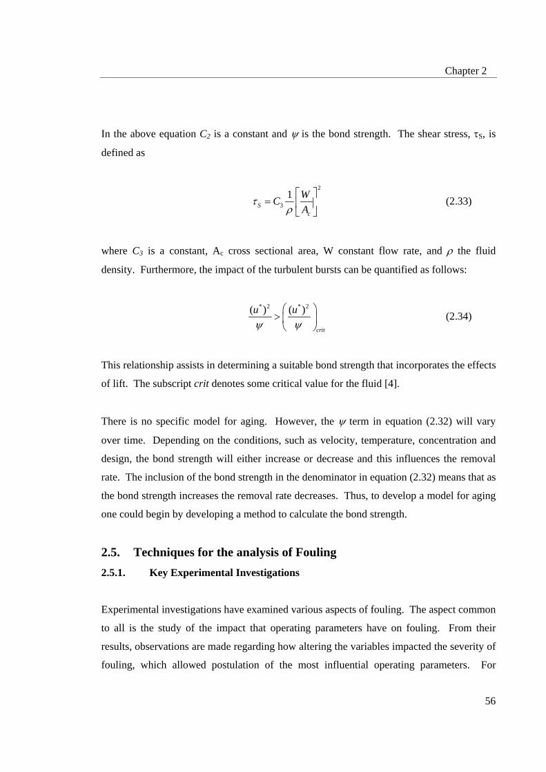
Chapter 2

56

In the above equation C2 is a constant and ψ is the bond strength. The shear stress, τS, is

defined as

2

31

Sc

WCA

τρ

⎡ ⎤= ⎢ ⎥

⎣ ⎦ (2.33)

where C3 is a constant, Ac cross sectional area, W constant flow rate, and ρ the fluid

density. Furthermore, the impact of the turbulent bursts can be quantified as follows:

* 2 * 2( ) ( )

crit

u uψ ψ

⎛ ⎞> ⎜ ⎟

⎝ ⎠ (2.34)

This relationship assists in determining a suitable bond strength that incorporates the effects

of lift. The subscript crit denotes some critical value for the fluid [4].

There is no specific model for aging. However, the ψ term in equation (2.32) will vary

over time. Depending on the conditions, such as velocity, temperature, concentration and

design, the bond strength will either increase or decrease and this influences the removal

rate. The inclusion of the bond strength in the denominator in equation (2.32) means that as

the bond strength increases the removal rate decreases. Thus, to develop a model for aging

one could begin by developing a method to calculate the bond strength.

2.5. Techniques for the analysis of Fouling 2.5.1. Key Experimental Investigations

Experimental investigations have examined various aspects of fouling. The aspect common

to all is the study of the impact that operating parameters have on fouling. From their

results, observations are made regarding how altering the variables impacted the severity of

fouling, which allowed postulation of the most influential operating parameters. For

Chapter 2

57

example, Bansal [20] through examination of the influence that operating parameters had

on the fouling rate determined that the deposition rate was increased with higher

temperatures and higher solution concentration. Another key objective in these

experimental studies is to determine the dominant process and controlling mechanisms.

For example, a study by Helalizadah [14] into crystallisation fouling in an annular test

section postulated the impact of varying operating parameters on the controlling process.

Most notably it was noted that the crystallisation fouling was reaction-controlled at higher

velocities but became diffusion controlled as the velocity decreased, which increased the

thickness of the hydrodynamic boundary layer.

Key observations regarding the most influential operating parameter or the most dominate

mechanism led to the development of empirical models. Most of these were presented in

Table 2.1. Another example, Ritter [1] examined the fouling results for two salts and

developed separate empirical models through the correction of the result with six possible

parameters. For the first salt he placed the fouling rate as a function of the supersaturation

ratio squared and the mass transfer coefficient. For the second salt, the empirical model

derived for the fouling rate was a function of the supersaturation and the surface

temperature. The difference was justified by the fact that the second salt was determined to

be reaction-rate controlled (temperature dependant) while the first was diffusion or mass

transfer controlled. A final example of such efforts to use experimental investigation to

first examine the influence of key parameters then use the results to evaluate a empirical

model predictive models is presented by Mori [48]. These are the main aspects that

experimenters deduce from their results.

2.5.2. Using CFD to Investigate fouling

A number of recent fouling studies have emerged that use CFD to examine components of

the fouling phenomena. Studies like that of Kho [11] and Grijspeerdt [18], use CFD to

evaluate the behaviour of the velocity and temperature within their chosen geometry. The

authors analyse the resulting CFD solutions to hypothesis how the observed transport

characteristics would impact the fouling phenomenon. Such studies do not include models

Chapter 2

58

of the processes involved in fouling. There are two studies that do model the fouling

processes by employing the CFD solutions in empirical resistance-based fouling models.

The first, Mwaba [6], formulates a three-dimensional conduction problem to determine the

impact that a crystal layer depositing on one section of the geometry has on the simulated

temperature field. In the second, Brahim [5] obtains CFD solutions of the velocity field as

well as the temperature field in his investigation that numerically models calcium sulphate

fouling. Utilizing the empirical models of various fouling processes, he simulates the

growth of the crystal layer and achieves an estimate for the temporal behaviour of the

overall fouling resistance. However, Brahim only considers a fictitious growth of the

crystal layer rather than the actual growth because of the complexity involved in altering

the geometry when considering actual or real crystal growth [5]. The “fictitious” method

maintained an unaltered geometry for the duration of the simulation but altered the inlet

velocity in accordance with the crystal layer. The concept of complexity was reinforced in

Grijspeerdt’s comment stating that the difficulty in modelling the fouling phenomena

relates to the fact that the processes involved are intrinsically dynamic [18]. Despite this

justifiable complexity, the research detailed in this paper includes many of the fouling

processes within the CFD component in an effort to describe the effect that real crystal

growth has on the behaviour of the transport variables.

2.5.3. Advantages of Using CFD over Experimental Techniques

Essentially, the experimental approach does provide important information to the

researcher but is limited in the level of detail it is able to achieve. On the other hand, the

CFD approach is capable of providing a greater level of detail. For example, the

experimental technique is restricted to assessing the impact of changing conditions by

examining their overall effect. The CFD technique allows analysis to be conducted on the

impact of operating parameters at a local scale and to determine whether the impact varies

in different regions of the chosen geometry. Obtaining the same level of details

experimentally would require more intrusive techniques that may actually affect the studied

phenomena. For example, a transparent window could be inserted in a heat exchanger to

observe the transient development of a deposit by inserting on the heat exchanger [13].

Chapter 2

59

However, since the window would have different surface properties to the metal, it is likely

fouling material will deposit on the window. Other experimental tools such as

thermocouples inserted into the geometry and any protrusions holding such tools in place

would most likely influence transport characteristics, like the hydrodynamics, which dictate

any deposition. There do exist other, more non-intrusive techniques like laser techniques,

radioactive tracers and moving pictures but they are not commonly used due to their

expense. Hence, CFD provides a relatively cheap technique that is completely non-

intrusive and capable of detailing the interactions of parameters on a local scale.

2.6. Closing Statement

The literature review has introduced the concept of fouling and its key characteristics. This

was followed by an extensive outline of the main fouling models and the different

techniques used to predict its transient behaviour. The resistance-based models are the

most established technique that provides details on the global influence of operating

parameters. The Lagrangian and the Eulerian method both provided a closer examination

of various fouling aspects. However, there existed no comprehensive model predicting the

fouling behaviour. This is despite the growth of fouling investigation using numerical

techniques and, in particular, the CFD approach. The CFD method presents an opportunity

to detail intricate interactions of the various phenomena associated with fouling. The CFD

technology will provide the necessary tools to detail these interactions and, ultimately,

provide an understanding of fouling that is of practical use. Hence, this research is capable

of delivering the alternate methodology that Karabelas [2] called for in his review of

current fouling research priorities.

Chapter 3

60

3. Materials Equation Chapter 3 Section 1

This chapter describes the tools required for both the development and assessment of the

numerical model. The first part of the chapter introduces the numerical technique used and

the software employed for the model development. The following section examines the

tools used to assess the adequacy of the resulting model. A specific strategy has been

selected to ensure each stage of the model is properly evaluated and the likely sources of

error established. This strategy will assist in identifying areas needing improvement in a

model that will become complex in the latter stages of development.

3.1. Computational Fluid Dynamics – An introduction

Computation Fluid Dynamics (CFD) is the numerical modelling of systems that exhibit

fluid flow, heat transfer and mass transfer [49]. The basis for the analysis is the derivation

of equations governing the conservation of the fluid flow, heat transfer and mass transfer

over a given domain of interest. The resulting conservation equations are reminiscent of

the partial differential equations associated with the Naiver Stokes equation. To

numerically solve these equations, they need to be transformed into a finite algebraic form.

Once in this form the equations are then solved using a computer following the

specification of the flow domain and the conditions within. Following the solving of the

numerical equation, the CFD solutions are capable of returning a complete picture of the

behaviour of fluid flow and the other phenomenon under given conditions [50]. It is a very

powerful technique that has far reaching applications in both industrial and non-industrial

areas [49].

It is the ability for the CFD method to return a complete picture of the behaviour of fluid

flow, heat transfer and mass transfer that makes it the method of choice for this research.

Traditionally, experimental methods have been used to investigate fouling. However, as

the literature survey showed, the use of CFD in fouling research is a growing area. The

most obvious reason is in its ability to visualize the complete phenomenon within the

process unit of interest. The ability to visualize allows either the examination of the

Chapter 3

61

variation of flow characteristics within a geometry in relation to the distribution of the

deposit [11] or, for similar purposes, examining the heat transfer characteristics [18]. In

both cases the detail was used firstly to understand the effect a given variable, like velocity,

had on the fouling phenomena and, secondly, as a guide for improving design to minimize

the fouling. The ideas fit into the key objective of this research of creating a predictive

model. One must have a detailed understanding of the intricate interactions are involved

within a process unit experiencing fouling in order to predict such a complex phenomena.

Brahim [5] states another reason being that CFD simulations offer a fast prediction of the

fouling phenomena. This is no doubt relative to the experimental approach.

To use the CFD method required various materials as well as a basic knowledge. For this

research project, which started in 2001, the commercial CFD code of choice was CFX-4.3.

Its internal structure of information made customizing the model a relatively

straightforward task, particularly for an inexperienced user. The commercial code can be

customized through the coding of additional subroutines in the computer language of

Fortran. Hence, the second software required was that of Visual Fortran, which provided a

compiler compatible with the CFD code. In June 2004 CFX-5.7 was released and provided

additional capabilities that were of interest to the investigation. As a result, upon release,

CFX-5.7 was used as the commercial CFD code. It also required the use of Visual Fortran

to customize the code to model aspects of the fouling phenomenon via functions and

subroutines. In terms of hardware a Pentium 3 was used for CFX-4.3 while the upgrade to

a Pentium 4 coincided with the release of CFX-5.7. The focus of the project was centered

on developing extensive subroutines to model the fouling phenomena and, hence, a PC

proved satisfactory in most cases.

3.2. The Strategy for Validation of the fouling model

Validation is the process used to determine whether the development CFD model

adequately represents the real process, which it is attempting to simulate. Formally, it is

defined as the process which ensures the code is “solving the right equations” [51]. The

procedure involves examining various aspects of the numerical solutions. This may include

Chapter 3

62

determining the suitability of chosen numerical methods or equations as well as evaluating

the appropriateness of applied boundary conditions. The most common form of evaluation

is the comparison of the numerical solutions with experimental results. The model that is

developed, as part of this investigation, will be analysed with respect to these aspects where

possible. However, the comparison with experimental data is often considered to be the

main step in the validation.

A two-step form of this validation is adopted within this research. The first involves

comparing the numerical solutions for the basic transport processes with established

empirical relationships. The purpose is to determine whether the selected equations

correctly model the transport phenomenon before increasing the complexity by including

the fouling components of the model and, thus, increasing its complexity. The relevant

empirical correlations for momentum, heat and mass transfer are briefly outlined below.

The second step compares the results of the model components which consider fouling

process. The numerical results are compared with the data obtained from experimental

fouling investigations, detailed below, to ensure the quality of the model’s fouling aspects.

Essentially this strategy is considered ideal for the intended complexity of the model as it

methodically identifies possible sources of error, which will assist in a better evaluation of

the final model.

3.2.1. Transport Phenomena: Empirical Correlations

The hydrodynamic characteristic of the numerical solutions will be assessed through

comparing the values of the friction coefficient. The numerical solution for the shear stress

at a solid boundary can be combined with the bulk velocity to calculate the fiction

coefficient, show in equation (3.1).

212

wf

m

Cu

τρ

= (3.1)

Chapter 3

63

The ability of CFD solutions to describe the local hydrodynamic characteristics means that

Equation (3.1) can be used to calculate the distributed of the friction factor along a solid

boundary. To validate the results a corresponding empirical model is required. For

example, a common geometry used in the investigation of heat exchanger fouling is tubular

geometry and the turbulent flow regime is often the regime of interest. An empirical

correlation that describes the friction factor under these conditions for fully developed flow

is defined in Equation (3.2) [52].

1 50.184 Ref −= (3.2)

The values calculated from Equation (3.2) are only valid over the following range:

[ ]10, 000 Re 100, 000≤ ≤ (3.3)

Finally, the friction coefficient is calculated by substituting the value obtained from

Equation (3.2) into Equation (3.4) and the resulting value compare with the obtained from

the numerical solutions.

4ffC = (3.4)

This examination could also assist in the selection of the most suitable turbulent model.

Other expressions can be found for differing geometry and ranges as well as for laminar

flow.

A variable often used in validating the heat transfer characteristics is the Nusselt Number.

There are two main correlations for the fully developed Nusselt number. These define the

heat transfer characteristics in turbulent flow. The first is the Colburn equation (Equation

(3.5)).

4 5 1 30.023 Re PrNu = (3.5)

Chapter 3

64

The second and preferred version of the Colburn equation is the Dittus-Boelter relationship

(Equation (3.6)). It differs only slightly from the Colburn equation and is of the form.

4 50.023 Re PrnNu = (3.6)

where n = 0.4 for heating (TSurf>Tm) and 0.3 for cooling (TSurf<Tm). These equations have

been confirmed experimentally for the range of conditions.

0.7 Pr 160Re 10, 000

10LD

⎡ ⎤⎢ ⎥≤ ≤⎢ ⎥

≥⎢ ⎥⎢ ⎥

≥⎢ ⎥⎣ ⎦

(3.7)

Equation (3.8) is used to obtain a value for the heat transfer from the numerical solutions by

considering the local heat flux with the corresponding wall and bulk temperatures.

( )Surf m

qhT T

′′=

− (3.8)

The mass transfer coefficient is then use to calculate a corresponding numerical value for

the Nusselt number. Caution needs to be taken to determine whether the heat transfer

coefficient calculated in Equation (3.8) represents fully developed thermal conditions. To

obtain a sound validation the conditions experienced within the numerical results must

correspond with those used in deriving the empirical correlations. The local values of the

heat transfer coefficient calculated from the numerical data are plotted against their position

on the solid surface to determine whether or not those represent the fully developed case.

Fully developed thermal conditions are attained when the local heat transfer coefficient is

constant and independent of position along the solid surface.

Chapter 3

65

The mass transfer phenomenon is the last characteristic to be examined and the mass

transfer coefficient is the variable considered when examining the mass transfer

characteristics. From the numerical results, it is calculated based on the local mass

concentration values at the wall and in the bulk as well as the corresponding value wall

mass flux (Equation (3.9)). However, the mass transfer coefficient can only be calculated if

there exists a mass flux within the CFD simulation.

( )mSurf m

JkC C

=−

(3.9)

It is important to establish the significance of the mass transfer coefficient in the context of

the fouling phenomenon to demonstrate the significance of selecting the most suitable

empirical correlation. A key aspect in experimental investigations of the fouling

crystallisation mechanisms is the determination of the kinetic data associated with the

investigated process. To determine the kinetic data, two components of the previously

described resistance-based models are combined. The first represents the transportation

process (Equation (3.10)):

( )d m b Sk C Cφ = − (3.10)

The second represents the surface attachment (Equation (3.11)) process:

( ) rxnnd R S Satk C Cφ = − (3.11)

These two equations combine to describe the net depositions of the crystallisation

mechanism. There exist two unknown variables in Equation (3.10) and Equation (3.11),

the surface concentration and surface reaction rate constant. The variable of interest is the

surface reaction rate constant. Therefore Equation (3.10) and Equation (3.11) are

rearranged to eliminate the surface concentration. In doing this, the crystallisation

phenomena defined in Equation (3.11) is considered a 2nd order reaction as is confirmed by

various experimental investigations [53]. Lastly, the mass transfer coefficient within

Chapter 3

66

Equation (3.10) is assumed to be a known variable, calculated from a selected Sherwood

number. Following the inclusion of these variables, the rearrangement and factorization,

Equation (3.12) is the resulting equation from which the reaction rate constant is calculated.

( )

( )2

@

12

14

ind

mb Sat

Rff f m

t m mb Sat

R R

k C CkdR

k kdt k k C C

k k

ρ

⎡ ⎤⎛ ⎞+ − −⎢ ⎥⎜ ⎟

⎝ ⎠⎢ ⎥= ⎢ ⎥

⎛ ⎞ ⎛ ⎞⎢ ⎥+ −⎜ ⎟ ⎜ ⎟⎢ ⎥

⎝ ⎠ ⎝ ⎠⎣ ⎦

(3.12)

In Equation (3.12) the value of the deposition rate is calculated from the initial growth rate

of the fouling resistance for a dynamic fouling run [54]. The value of the deposition rate is

attributed to an average surface temperature that is estimates as a constant value. The

deposition rate together with a mass transfer coefficient is then inserted into Equation

(3.12) and a rate constant is calculated. Hence, the calculated rate constant represents the

surface temperature that was attributed to the deposition rate. A number of rate constants

can be calculated if fouling rates are obtained for different surface temperatures. The

resulting array of rate constants and their corresponding surface temperature values are

used in an Arrhenius relationship to estimate kinetic data for the crystallisation.

In this particular discussion the main point of interest is the mass transfer coefficient used

in Equation (3.12). This is because there exists a variety of Sherwood correlations that

describe the same mass transfer characteristics. The resulting value of the reaction rate

constant depends on the selection of the Sherwood correlations used to calculate the mass

transfer coefficient. Values for the mass transfer coefficient are obtained from published

Sherwood number correlations. Similarly to the correlation for the Nusselt number, the

Sherwood number correlations depend on flow conditions and geometry [6]. The

correlation that was used in the literature, which derived Equation (3.12), follow [54, 55]:

0.875 0.330.034 Re ScSh = (3.13)

Chapter 3

67

The correlation defined in Equation (3.13) was based on experimental investigations

examining crystallisation fouling on a heating surface [55]. This correlation has been used

to define mass transfer characteristics in both annular [54] and rectangular [5] geometry. It

requires calculating the viscosity of a CaSO4 solution and the diffusivity of CaSO4 in water.

An alternate correlation used by Mwaba [6] for the same purpose is defined in Equation

(3.14).

0.8 0.33 60.023 Re Sc 1 hdShx

⎛ ⎞= +⎜ ⎟⎝ ⎠

(3.14)

Equation (3.14) takes into account the impact of entrance effects [6] in a tubular geometry.

These entrance effects are accounted for in the final term. They appear to dependant on

both the hydraulic diameter and the displacement from the entrance. It is assumed that the

other component describes conditions for fully developed flow, as it appears similar to a

variety of empirical correlations for the Sherwood number. These correlations consider a

similar mass transport phenomena to that encountered by Mwaba [6] but for fully

developed turbulent flow in tubular geometry. The first of these is the Chilton j-factor

analogy [56]:

0.171 3 0.023 Re

Re ScDShj −= = (3.15)

Another represents turbulent flow in tubes and is a modified Gilliland and Sherwood

correlation for liquids [56]:

0.83 0.440.023 Re ScSh = (3.16)

Finally, there is the Dittus-Boelter Analogy [52] which can be used by considering the n

coefficient being equal to 0.3, the value corresponding to the occurrence of deposition

(Cs<Cm)):

Chapter 3

68

4 5 0.30.023 Re ScSh = (3.17)

Equation (3.17) is included to emphasis the diverse range of possible correlations that can

be used to define the mass transfer coefficient.

Where a mass flux is specified within the CFD model, the numerical value for the fully

developed mass transfer coefficient (Equation (3.9)) will be compared with corresponding

values obtained from Equations (3.13)-(3.17). It is expected these empirical correlations

will return a range of values for the same conditions because differences can be observed in

the form and the coefficients of the various empirical correlations. This makes obtaining a

conclusive result from the validation difficult to perform. Hence, the objective is to assess

which empirical correlation best corresponds with the mass transport phenomena depicted

in the CFD model.

3.2.2. Fouling Processes: The Experimental Data

Having used the empirical correlations to assess the numerical results for the transport

phenomena the next stage of the validation is to examine the fouling components of the

model. This is done through obtaining suitable fouling experimental results to assist in

both the model development and the comparison. There exist two difficulties in attempting

this validation. The first is obtaining data from experimental runs that correspond to the

numerical simulations visa versa. The second difficulty is obtaining a set of experimental

results that enable a comprehensive validation of the modeled fouling phenomena.

Valiambas [57] conducted a study outlining the information required to achieve a complete

set of fouling data which would achieve the desired comprehensive model validation.

However, the study found that there generally does not exist a complete set of such data

[57]. Interestingly, three of the four vital areas where there exists an insufficient amount of

data would be most suited for the purpose of validating CFD solutions. These areas of

deficiency include a lack of measurement of deposit properties and the lack of data to

assess the possible variation of deposition rate along the flow path. Another problem was

that the existing fouling data covered a relatively narrow range of both flow velocities and

Chapter 3

69

wall temperatures. To possess a more complete set of data would be most advantageous in

this investigation considering that the CFD solutions give results of the behavior of

operating parameters on a local scale.

It was fortunate that this investigation was able to obtain two separate sets of experimental

data, which could be used at different stages of model development. The first set of

experimental results obtained is for the thickness distribution of the final deposit along the

heat transfer surface (Figure 3.1). The results are for an annular duct where the heated

section if the inner surface and flow enters with low turbulent Reynolds number to

minimize the occurrence of removal.

0.0000

0.0005

0.0010

0.0015

0.0020

0.0025

0.0030

0.0035

0.0040

0.0 0.4 0.8 1.2 1.6Length m

Expe

rim

enta

l Thi

ckne

ssm

Figure 3.1 – Experimental results [58] representing the distribution thickness of the deposit along the heat

transfer surface.

The second set of data is a collection of fouling curves obtained for the same run but from a

number of thermocouples distributed along a heated section. This experimental data used

in this paper is part of ongoing work of Fahiminia from the University of British Columbia,

Canada. His assistance is greatly appreciated [59]. The run was conducted over a 32-hour

period to investigate fouling of calcium sulphate within a tubular geometry. The geometry

was 0.772 m long and had an inner diameter of 9.02 mm. Calcium sulphate in pure water

was used as the crystalline system. The inclusion of thermocouples distributed at different

Chapter 3

70

intervals along the external surface of the tubular geometry allowed Fahiminia to monitor

the local behavior of fouling through its resistance over time. These results are beneficial

because their local nature is compatible with the abilities of CFD. The fact that Fahiminia

used thermocouples to obtain local fouling curves reflects the sentiment expressed by

Karbaelas [2] that a more intimate understanding of fouling is required. An example of the

results is presented in Figure 3.2. Figure 3.2 shows essentially three sections of the run

namely, the nucleation time, the roughness delay time and the fouling period. In addition,

the observed linear fouling rate leads to the assumption that removal of the fouling film is

negligible. Finally, a fine filter was used and the assumption is made that only

crystallisation fouling occurs. These experimental results included data for the initial and

final values of surface temperature as well as induction time estimates at each

thermocouple. It is noted that the geometry is different for the two data sets and, thus,

requires the numerical model to be altered accordingly.

-6 2Fouling Rate = 4.85×10 m K/kJ

The Fouling Period

RoughnessDelay Time

Nucleation Time

Figure 3.2 – Experimental results [59] of the changing fouling resistance over time obtained at the 10th

Thermocouple. This fouling curves displays two fouling processes the induction period and the fouling

period. The induction period includes a nucleation period and a roughness-delay period.

Finally, various experimental results, both quantitative and qualitative, from literature

concerned with fouling [1, 20, 22, 28] will be used during the model development. Other

data required concerns relationships for the kinetic [54] and thermodynamic [60, 61]

behavior.

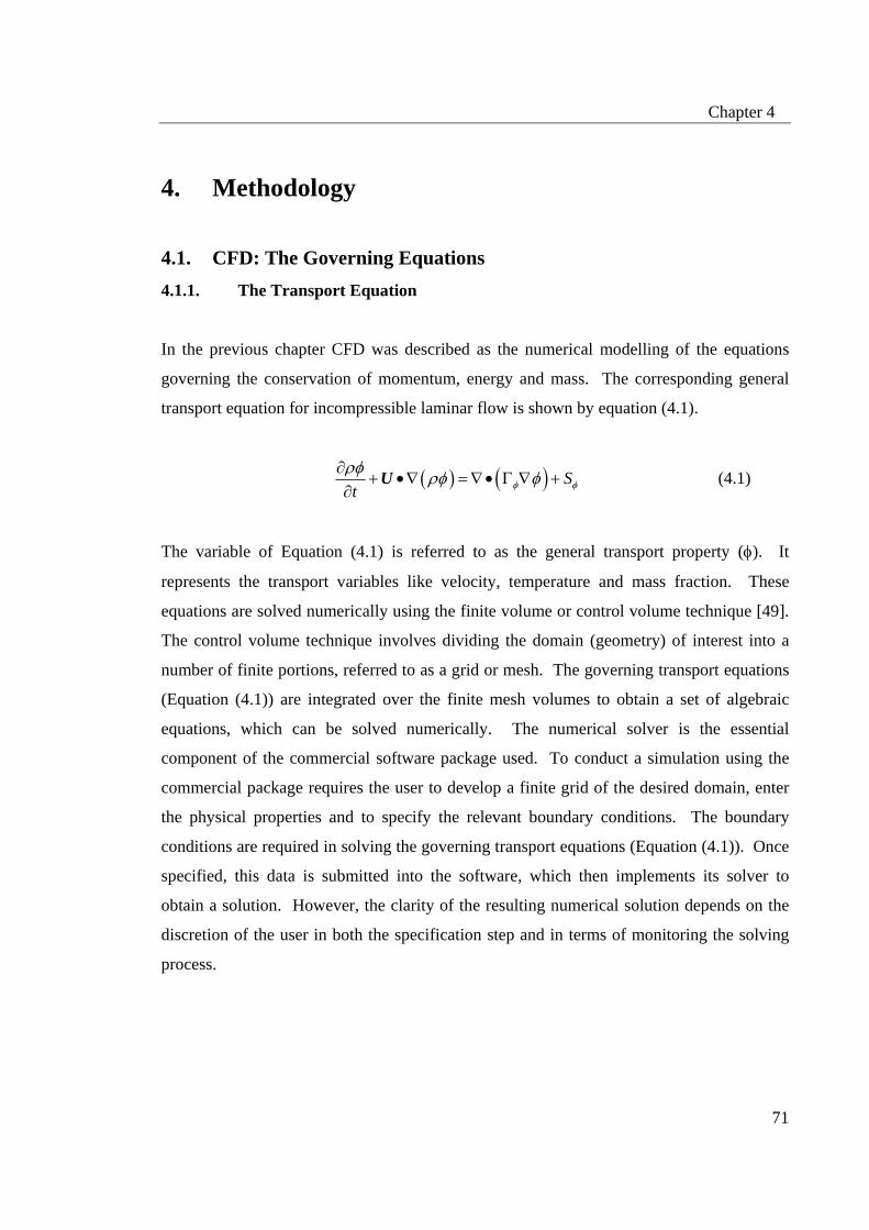
Chapter 4

71

4. Methodology Equation Chapter 4 Section 1

4.1. CFD: The Governing Equations 4.1.1. The Transport Equation

In the previous chapter CFD was described as the numerical modelling of the equations

governing the conservation of momentum, energy and mass. The corresponding general

transport equation for incompressible laminar flow is shown by equation (4.1).

( ) ( ) St φ φ

ρφ ρφ φ∂+ •∇ = ∇ • Γ ∇ +

∂U (4.1)

The variable of Equation (4.1) is referred to as the general transport property (φ). It

represents the transport variables like velocity, temperature and mass fraction. These

equations are solved numerically using the finite volume or control volume technique [49].

The control volume technique involves dividing the domain (geometry) of interest into a

number of finite portions, referred to as a grid or mesh. The governing transport equations

(Equation (4.1)) are integrated over the finite mesh volumes to obtain a set of algebraic

equations, which can be solved numerically. The numerical solver is the essential

component of the commercial software package used. To conduct a simulation using the

commercial package requires the user to develop a finite grid of the desired domain, enter

the physical properties and to specify the relevant boundary conditions. The boundary

conditions are required in solving the governing transport equations (Equation (4.1)). Once

specified, this data is submitted into the software, which then implements its solver to

obtain a solution. However, the clarity of the resulting numerical solution depends on the

discretion of the user in both the specification step and in terms of monitoring the solving

process.

Chapter 4

72

4.1.2. The Turbulence models

Equation (4.1) represents the laminar form of the transport equation. To evaluate the

turbulent form of Equation (4.1) requires the performing of a step known as time averaging

[49]. Essentially, it involves breaking down the velocity into two components. One

represents the mean value and the other is a representation of the fluctuations that are

characteristic of turbulent flow. Equation (4.2) is the result of this transformation.

( ) ( )( ) ( )T u u pt

ρ ρ µ ρ∂ ⎡ ⎤ ′ ′+ •∇ = ∇ • ∇ + ∇ + ∇ • − − ∇⎢ ⎥⎣ ⎦∂U U U U U (4.2)

The main difference between the laminar form of the velocity equation (Equation (4.1)) and

its turbulent form (Equation (4.2)) is the appearance of the second term of the right hand

side of Equation (4.2). This term is representative of the turbulent stresses and is referred

to as the Reynolds Stresses. These are additional to the viscous stresses, which are

prominent within the boundary layer and also appear in the laminar form of the equation.

For the three dimensional form of the equations, the Reynolds Stresses creates six extra

unknowns which make the equations difficult to solve directly as the number of unknowns

out number the number of equations. These extra unknowns are evaluated based on a

theory developed by Boussinesq (1877). For incompressible flow, one recalls Newton’s

law of viscosity, which states that the viscous stress is proportional to the rate of

deformation:

jiij ij

j i

uue

x xτ µ µ

⎛ ⎞∂∂= = +⎜ ⎟⎜ ⎟∂ ∂⎝ ⎠

(4.3)

Boussinesq (1877) developed an analogy for the Reynolds stress stating that the Reynolds

stress was also related to the rate of deformation but utilized a value of the turbulent

viscosity as the proportionality constant:

Chapter 4

73

jiij i j T

j i

uuu ux x

τ ρ µ⎛ ⎞∂∂′ ′= − = +⎜ ⎟⎜ ⎟∂ ∂⎝ ⎠

(4.4)

Using this relationship the values of the Reynolds Stresses can be approximated and, hence,

solved for the turbulent equations for motion. An analogy of Equation (4.4) can be applied

to the general case in the form of the Eddy Diffusivity Hypothesis (Equation (4.5)).

TT

T

u µρ φ φ φ

σ′ ′− = Γ ∇ = ∇ (4.5)

The task now becomes deriving expressions to calculate the turbulent viscosity, µT, which

appears in Equation (4.4) and Equation (4.5). Hence, to complete the description of the

Reynolds shear stresses requires defining the turbulent viscosity. The k-ε model turbulent

model provides an algebraic definition to the turbulent viscosity, µT, and brings closure to

the turbulent form of the transport equations. The Low Reynolds number k-ε model and

the standard k-ε model number, which uses scalable wall functions, are two forms of the

models that will be used in this research.

4.1.2.1. The Standard k-ε model

One of the most prominent turbulence models, the k-ε (k-epsilon) model, has been

implemented in most general purpose CFD codes and is considered the industry standard

model [49]. It has proven to be stable, numerically robust and has a well-established regime

of predictive capability. For general-purpose simulations, the k-ε model offers a good

compromise in terms of accuracy and robustness. This turbulent model defines turbulent

viscosity, µT, using the following algebraic expression:

2

TkCµµ ρε

= (4.6)

Chapter 4

74

Furthermore, the k-ε model uses the turbulent viscosity, µT, in an Extended Boussinesq [49]

approach to define the Reynolds stress:

23

223

jii j T ij

j i

T ij ij

uuu u kx x

E k

ρ µ ρ δ

µ ρ δ

⎛ ⎞∂∂′ ′− = + −⎜ ⎟⎜ ⎟∂ ∂⎝ ⎠

= −

(4.7)

Substituting the Extended Boussinesq expression (Equation (4.7)) for the Reynolds stresses

into the velocity transport (Equation (4.2)) gives:

( ) ( )( )

( )( ) 23

Tsol sol

TT sol

t

p k

ρ ρ µ

µ ρ

∂ ⎡ ⎤+ •∇ − ∇ • ∇ + ∇ =⎢ ⎥⎣ ⎦∂⎡ ⎤−∇ + ∇ • ∇ + ∇ −⎢ ⎥⎣ ⎦

U U U U U

U U δ (4.8)

To calculate the turbulent viscosity and solve Equation (4.7), values for the turbulent

kinetic energy and the dissipation, variable that appears in the k-equation, are required.

The dissipation of turbulent kinetic energy is the work done by the smallest eddies against

the viscous stresses. Therefore, the k-ε model introduces two new variables into the system

of equations. The values of k and ε come directly from the differential transport equations

for the turbulence kinetics energy and turbulence dissipation rate:

( ) Tk

k

k k k Pt

µρ ρ µ ρεσ

⎡ ⎤⎛ ⎞∂+ ∇ • = ∇ • + ∇ + −⎢ ⎥⎜ ⎟∂ ⎝ ⎠⎣ ⎦

U (4.9)

( ) ( )1 2T

kC P Ct k ε ε

ε

µρε ερ ε µ ε ρεσ

⎡ ⎤⎛ ⎞∂+ ∇ • = ∇ • + ∇ + −⎢ ⎥⎜ ⎟∂ ⎝ ⎠⎣ ⎦

U (4.10)

( ) ( )2 33

Tk T T kbP U k Pµ µ ρ= ∇ • ∇ + ∇ − ∇ • ∇ • + +U U U U (4.11)

Chapter 4

75

The interesting component of this two-equation turbulence model is in its use of wall

functions to evaluate the behavior within the viscous sub-layer. These wall functions have

been calibrated to model the universal behavior of near-wall flows:

( )1 ln pUu Eyuτ κ

+ += = (4.12)

pp w

yy ρτ

µ+ = (4.13)

However, there exists a problem in the standard wall function approach when the objective

is to model additional variables, which have a higher Schmidt number. As will be

described in the remainder of this methodology it is the aim of this investigation to model

additional scalar variables with a relatively high Schmidt number. The problem with the

standard wall functions concerns the specification of the scalar version of the E variable,

which appears in Equation (4.12):

0.75

Pr Prexp 9.0 1 1 0.28exp 0.007E E φ φ

φφ φ

κσ σ

⎛ ⎞⎛ ⎞⎛ ⎞⎛ ⎞ ⎛ ⎞⎜ ⎟⎜ ⎟= − + −⎜ ⎟⎜ ⎟ ⎜ ⎟⎜ ⎟ ⎜ ⎟⎜ ⎟⎜ ⎟⎜ ⎟⎝ ⎠ ⎝ ⎠⎝ ⎠⎝ ⎠⎝ ⎠ (4.14)

In Equation (4.14), the value of Eφ has an upper limit 5.0×1035 meaning that it is incapable

of modelling phases that posses a high molecular Prandtl number. The intended additional

phases have what is considered a high molecular Prandtl number of around 400 and are

therefore more compatible with the standard wall functions. However, the standard k-ε

turbulence model in the June 2004 release of CFX-5.7 uses the scalable wall functions.

The scalable wall function method is an improvement on the standard wall functions in

terms of their robustness and accuracy when the near-wall mesh is very fine. Most

importantly these improvements enable the following scalable wall functions to model

Chapter 4

76

phases that have a high molecular Prandtl number. These scalable wall functions are

outlined in Equations (4.15) to (4.17).

1 4 1 2*u C kµ= (4.15)

( )1 log *tU y Cuτ κ

= + (4.16)

( )* *y u yρ µ= ∆ (4.17)

Of additional usefulness is the ability the scalable wall functions have to be modified to

incorporate the case of a rough surface. For rough walls, the same logarithmic profile

exists, but is adjusted so the wall moves closer under the same inlet flow conditions. This

is accounted for by modifying the equation (4.16) as follows:

1 *ln1 0.3

tU y Cu kτ κ +

⎛ ⎞= +⎜ ⎟+⎝ ⎠ (4.18)

where the non-dimensional expression for roughness, k+, is defined as:

*Rk y uρµ

+ = (4.19)

In Equation (4.19), the dimensionless roughness, k+, is a function of the equivalent sand

grain roughness, yR. As explained in the literature review, the equivalent sand grain

roughness is the same as surface roughness that was established by Moody [33]. Caution

needs to be taken when specifying the equivalent sand grain roughness within the

commercial code as instabilities can arise if its value is of the same order or larger than the

distance from the wall to the first mesh point [62].

Chapter 4

77

4.1.2.2. The Low Reynolds number k-ε model

The wall function approach operates well when the Reynolds number is high and the

resulting viscous effects are unimportant [63]. Although, when a lower turbulent Reynolds

number is applied the viscous stresses are more influential and the function approach is not

as suitable. Thus, the Low Reynolds number turbulent k-ε model was proposed to deal

with the Reynolds number range of 5,000 to 30,000. Unlike the standard version, the low

Reynolds number version is able to integrate through the boundary layer by its use of

various assumptions and functions [63]. These functions are known as dampening

functions, which are used to ensure that viscous stress take over from the Reynolds stresses

within the near wall region [49]. Patel [63] reviews eight different versions of the Low

Reynolds k-e model including the Launder-Sharma version. Basically, the difference

between these review models lies in their definition of the dampening functions. In the

commercial code used, the Launder-Sharma version is applied and it replaces Equations

(4.6)-(4.10) of the standard model with the following equations:

2

T solkC fµ µµ ρε

= (4.20)

( )

( ) ( )12

2: 2

Tsol sol

k

TT sol

k k kt

k

µρ ρ µσ

µ ρ ε µ

⎡ ⎤⎛ ⎞∂+ •∇ − ∇ • + ∇ =⎢ ⎥⎜ ⎟∂ ⎢ ⎥⎝ ⎠⎣ ⎦

⎡ ⎤∇ ∇ + ∇ − − ∇⎣ ⎦

U

U U U

(4.21)

( )

( )

( )

2

1 1 2 2

2

:

2

Tsol sol

TT sol

T

sol

t

C f C fk k

ε

ε ε

µρ ε ρ ε µ εσ

ε εµ ρ

µµρ

⎡ ⎤⎛ ⎞∂+ •∇ − ∇ • + ∇ =⎢ ⎥⎜ ⎟∂ ⎢ ⎥⎝ ⎠⎣ ⎦

⎡ ⎤∇ ∇ + ∇ − +⎣ ⎦

∇∇

U

U U U

U

(4.22)

Chapter 4

78

As with the standard k-ε model, the required boundary conditions that need specification

are essentially that at the inlet and the specification of conditions at the wall. To model the

flow entering fully developed the inlet is simply set, in CFX-4.3, as a mass boundary, the

mass flow specified and the velocity components are all extrapolated from upstream then

adjusted to fix desired mass flow rates [64]. However, a similar procedure is not used in

CFX-5.7. The specification of fully developed flow within CFX-5.7 involves the

generation of a fully developed velocity profile, which is then specified at the inlet. The

boundary conditions at the wall are similar with either a value or a flux requiring

specification. The only difference being that the Low Reynolds k-ε model in the

commercial codes used is the mobility to simulate roughness at the wall.

Finally, when using the Low Reynolds k-ε model, a developing flow can be modeled in

part due to the use of the dampening functions. However, the turbulent models do have

difficulty in their prediction of the transition involved in the development of flow [49] but

one can utilize the ability of the dampening functions to achieve a representation of

developing flow. To model the development of flow using the Low Reynolds number k-ε

turbulent model involves varying the turbulent parameters at the inlet to obtain a

development of the boundary layer along the path of the flow that is physically feasible and

correct. The turbulent parameters at the inlet that need specification are the dissipation

length (D) and turbulence intensity (I). These parameters are then used to specify the

turbulent kinetic energy (k), equation (4.23), and the specific dissipation rate (ε), equation

(4.24).

( )232 ink U I= (4.23)

34

32kC

Dµε = (4.24)

The difficulty arises in selecting the values of these parameters that result in the attainment

of a representation of the developing boundary layer that is physically sound. For example,

Chapter 4

79

the CFX manual states that using the hydraulic diameter in specification of the dissipation

length is not a good approximation when the inlet is as wide as the domain, when the

profiles of the turbulence quantities will be more important [65]. Furthermore, there is no

comprehensive theory of transition [49] because the transition that occurs in the

development of the boundary layer cannot be well predicted by the k-ε model [66]. To

resolve these problems and obtain suitable inlet conditions a method used in other

investigations [67, 68] is adopted. Simply, it is considered that the there exists a certain

degree of turbulence at the inlet, which is determined by conducting an analysis on the

dissipation length (D) and turbulence intensity (I). The analysis is essentially a calibration

that compares the resulting behaviour of the friction coefficient, a representation of the

developing boundary layer, with established theoretical data [69]. Finally it should be

noted that varying the level of turbulence in this matter does not impact on the degree of

turbulence that is present further downstream in the fully developed section of flow.

4.1.3. Verification Strategy

In the brief that defined the CFD methodology it was explained how the accuracy and

adequacy of the resulting numerical solution depends on the user’s discretion. One method

of ensuring that a high level of clarity is achieved is to adopt the strategy of verification.

Verification is an analytical method used to ensure that the governing “equations are solved

right” [51]. It involves assessing various aspects of the numerical simulation. There are

three main aspects of verification that are relevant to this study. The first concerns the

generation of a grid and obtaining an adequate spatial discretisation for the mesh points.

There exist a number of guidelines that should be followed to obtain a suitable grid.

However, these guidelines differ according to the flow models to be implemented. This is

particularly the case for the turbulent models. For example, the use of the standard k-ε

turbulent model requires a grid that has all mesh points outside the viscous sub-layer but

has have a minimum number of mesh points inside the boundary layer [70]. While for the

low Re k-ε turbulent model it is recommended that there is at least 15 mesh points for a

sub-layer [70]. The sub-layer has an approximate non-dimensional thickness (y+) of 60.

Therefore, to achieve suitable grids that follow these guidelines requires generation of grids

Chapter 4

80

that have their mesh points non-uniformly distributed to ensure they either do or do not

favor the laminar sub-layer, depending on the flow model used. The second aspect of the

verification is ensuring that a suitable level of iterative convergence and solution stability is

achieved. The final aspects relates to the intended transient simulations. The set-up of

transient simulations involves the specification of time steps, temporal discretisation. Each

of these verification steps requires a number of preliminary simulations to be conducted for

each component of the model. Therefore, the verification steps outlined here will be

followed in each stage of model development.

4.2. The Energy Transport Equation

One of the scalars to be modeled is temperature, which when substituted into the general

transport equation forms the following turbulent energy transport equation:

( ) ( )Pr

Tsol P sol P P

T

C T C T K T C Tt

µρ ρ⎛ ⎞∂

+ •∇ = ∇ • ∇ + ∇ • ∇⎜ ⎟∂ ⎝ ⎠U (4.25)

Equation (4.25) has utilized the Eddy Diffusivity Hypothesis (Equation (4.5)) to account

for the turbulence characteristics of the flow. Hence, the last term of Equation (4.25) does

not appear in the laminar version of the energy transport equation.

4.3. The Crystallisation Mechanism - Eulerian Modelling Approach 4.3.1. The Eulerian Modelling Approach to the homogeneous phase

This investigation is concerned with the modelling of the fouling mechanisms prominent in

saline streams associated with the desalination industry. A number of salts appear in the

streams and are involved in fouling. The simplest is calcium sulphate. It is considered to

be part of the equilibrium expressed in equation (4.26).

( ) ( ) ( )

2 24 4

R

aq aq sD

k

kCa SO CaSO+ − ⎯⎯→+ ←⎯⎯ (4.26)

Chapter 4

81

Equation (4.26) assumes that the combination of the two aqueous ions interact to form a

calcium sulphate precipitate. This is a simplification as the calcium sulphate can appear in

a transitional aqueous form as well as a solid precipitate form. Sparingly soluble salts such

as calcium carbonate or calcium phosphate have more complicated chemistry than this and

are also prominent salts found to cause fouling. However, the simplicity of the calcium

sulphate salt expressed in Equation (4.26) is most suitable in this investigation, whose

prime objective is on model development and the effects of operating parameters. More

complicated chemistry can be applied once the foundations of the model have been

produced.

The innovative part of this research is that the aqueous phase of equation (4.26) is included

in the CFD simulations as two additional transport equations, one for each species. The

general transport equation (Equation (4.27)) for the aqueous phase depicts the behavior of

the mass fractions of the species (αCa, αSO4).

( ) ( )Sc i

Tsol i sol i sol i i i

T

D St α

µρ α ρ α ρ α α⎛ ⎞∂

+ •∇ = ∇ • ∇ + ∇ • ∇ +⎜ ⎟∂ ⎝ ⎠U (4.27)

Equation (4.27) is the turbulent version and is for incompressible flow. As with the energy

transport equations, this species transport equations accommodates for the turbulence

behavior with the inclusion of the Eddy Diffusivity Hypothesis. Another characteristic of

Equation (4.27) is the substitution of the solution density for the fluid density. The solution

density is a function of the fluid density, the local mass fraction of the species and their

corresponding densities. The last term in Equation (4.27) is referred to as the source term.

It is noted that the high Schmidt number obtained from the aqueous species associated with

Equation (4.27) make the model incompatible with any turbulent model that uses standard

wall functions. This concept was raised in section 4.1.2.1. The turbulent models that are

therefore incompatible with this model set-up included the standard k-ε turbulent model

(CFX-4.3 version) and the Reynolds Stress equation model.

Chapter 4

82

4.3.2. Precipitation in bulk/boundary layer

Depending on conditions, calcium sulphate can be generated within the bulk/boundary

layer through the precipitation reaction from the aqueous phase as represented by Equation

(4.26). Equation (4.28) describes the 2nd order kinetic reaction that is usually used

associate with the calcium sulphate precipitation [53].

( )4ppt r soln spr k Ca SO kρ++ −−⎡ ⎤ ⎡ ⎤= −⎣ ⎦ ⎣ ⎦ (4.28)

The rate constant, kr, has an Arrhenius relationship [53] (Equation (4.29)) and the solubility

constant, ksp, (Equation (4.30)) is related to the solubility product and is a function of

temperature [64].

46.49×10

6 35.67×10 m mol.sRTrk e

−= (4.29)

12545.62log 390.9619 152.6264log 0.0818493SPk T TT

= − − + (4.30)

As previously mentioned the consideration of calcium sulphate is a simplification of a

saline stream and Equation (4.28) is the corresponding kinetic model. Equation (4.28) is

usually used in physical modelling the fouling kinetics of sparingly soluble salts [23]. To

model this precipitation in the CFD it will be incorporated into Equation (4.27). This is

simply done by specifying an adjusted form of Equation (4.28) as the source term. The

expression for the precipitation source term describing the consumption of both species of

the aqueous phase follows:

2-2+ 4

2+ 2-4

soln SOsoln Casp

Ca SOMW MWi rS k Kα

ρ αρ α⎛ ⎞⎡ ⎤⎡ ⎤⎜ ⎟⎢ ⎥= − −⎢ ⎥⎜ ⎟⎢ ⎥⎢ ⎥⎣ ⎦ ⎣ ⎦⎝ ⎠

(4.31)

Chapter 4

83

Equation (4.28) is based on the generation of particulate matter or the consumption of ions

in solution is generalized for either case as:

( )( )22 42 2

4 4

2 24

2solnsoln

soln 1i i

Ca SO

SOCar sp CaSO Ca SO

S MW k kMW MWα α

α α

ρ αρ αρ α α α

−+

+ −

+ −

⎛ ⎞⎡ ⎤⎡ ⎤⎜ ⎟⎢ ⎥ ⎡ ⎤⎢ ⎥= − − + +⎜ ⎟⎢ ⎥⎢ ⎥ ⎣ ⎦⎢ ⎥⎜ ⎟⎣ ⎦ ⎢ ⎥⎣ ⎦⎝ ⎠

(4.32)

To incorporate Equation (4.32) into the CFD involves the user writing a subroutine to alter

the source term of the transport equation for each species. CFX-4.3 allows the user to

specify the source terms through a Fortran subroutine known as USRSRC. An additional

function is coded for the solubility product, ksp, and called from within USRSRC. The code

can be found in Appendix B.

4.3.3. Crystallisation Fouling: Precipitation at the surface

Crystallisation Fouling is the result of the calcium sulphate precipitation occurring at the

surface (Equation (4.26)). The formed precipitant adheres to the surface forming a hard

and tenacious crystal deposit. This process is incorporated into the CFD through a

boundary condition imposed on the transport equations of the aqueous phases (Equation

(4.27)) at the solid-liquid interface of interest. The crystallisation fouling boundary

conditions is formulated in similar way to Equation (4.32) but is expressed as a flux (i

Jα )

per unit area and uses a surface reaction rate constant (kR):

( )

22 4

2 24

2 24 4

solnsoln

2

soln 1

Ca SOi

SOCa

Surf Surfi R

sp CaSO Ca SO Surf

MW MWJ MW k

k

α αα

ρ αρ α

ρ α α α

−+

+ −

+ −

⎛ ⎞⎡ ⎤⎡ ⎤⎜ ⎟⎢ ⎥⎢ ⎥ −⎜ ⎟⎢ ⎥⎢ ⎥⎜ ⎟⎣ ⎦ ⎢ ⎥= ⎣ ⎦⎜ ⎟⎜ ⎟⎡ ⎤⎛ ⎞− + +⎜ ⎟⎜ ⎟⎢ ⎥⎝ ⎠⎣ ⎦⎝ ⎠

(4.33)

Chapter 4

84

Equation (4.33) includes a reaction rate constant (Equation (4.34)) and the solubility

product (Equation (4.30)) for a calcium sulphate in a saline stream [64] (Ksp). Both depend

on the local temperature.

,0

A

surf

ERT

R Rk k e−

= (4.34)

The difficulty is that no data is available to describe the crystallisation surface kinetics in a

saline stream. An alternative is to consider the case of the Calcium Sulphate-Water System

(Equation (4.35)) where there exists satisfactory kinetic data [54] (Equation(4.36)).

( )2,i R sol i sol i satJ k ρ α ρ α= − (4.35)

44.04×10

4422.15 m kg CaSO .ssurfRT

Rk e−

= (4.36)

Equation (4.35) uses the saturation concentration [60] (Equation (4.37)) to describe the

solubility in the Calcium Sulphate-Water System. The saturation concentration expression

depends on the local temperature:

( ) ( )( )

4

3 2

, 0.00104 - 273.25 - 0.28772 - 273.25

16.74529 - 273.25 1839.83408

CaSO Sat Surf Surf

Surf

T T

T

α = ⋅ ⋅ +

⋅ + (4.37)

The kinetics values in Equation (4.36) are used as a basis for a validation study to assess the

appropriateness of the kinetic data describing crystallisation flux (Equation (4.33)) within a

saline stream. This study will be discussed in detail within the chapter investigating

precipitation fouling within saline waters.

To incorporate the crystallisation flux boundary condition into the CFD requires the coding

of another user subroutines. In CFX-4.3 the additional code is in the form of a subroutine

Chapter 4

85

known as USRBCS while in CFX-5.7 the boundary condition is entered as a CEL function.

In each case, the corresponding solubility relationships are coded as a separate user

function. These codes are submitted to the solver with the other simulation specifications.

4.4. The Particulate Mechanism Lagrangian Modelling Approach 4.4.1. The Lagrangian Modelling Approach to the discrete particulate phase

An alternate to the Eulerian Modelling approach used to describe the behavior of the

precipitated or particulate phase is the Lagrangian Modelling approach. It is used to

determine the trajectory of discrete particles formed within the aqueous phase. To derive

the Lagrangian equation (Equation (4.38)), the forces that act on a particle are taken into

account with the main force being the drag force.

( )218

pp Drag p D f p f p

dm d C

dtπ= = − • −

UF U U U U (4.38)

This ordinary differential equation (Equation (4.38)) is numerically solved for the trajectory

for a given particle. Solving Equation (4.38) requires the specification of the initial

position and velocity of the particulate matter as well as other characteristics including the

diameter, volume and an associated mass flow rate.

4.4.2. Particulate Generation: Precipitation within bulk/boundary layer

Modelling the particulate phase arises from the interest in assessing the likelihood of

composite fouling. Particular interest is placed on analyzing the impact of the particulate

matter that forms within the geometry. This objective motivated the development of a code

that interrelated the Eulerian and the Lagrangian modelling components. It is within the

Eulerian modelling component that the precipitation occurs through the consumption of the

aqueous phase (Equation (4.28)). However, it is the Lagrangian modelling component that

models the behavior of the discrete particulate phase, which forms as a result of this

precipitation reaction. In relating the two phases it was considered that the precipitation

Chapter 4

86

rate, the rate of particle production, is essentially the mass flow rate of the particulate

matter at the volumetric point of injection and, hence, a corresponding mathematical

relationship was formulated (Equation (4.39)).

( )( )

22 4

2 24,

2 24 4

solnsoln

,

2

soln 1

Ca SOCV i i

SOCa

p R CV i

sp CaSO Ca SO

MW MWm MW k V

k

α αα

ρ αρ α

ρ α α α

−+

+ −

+ −

⎛ ⎞⎡ ⎤⎡ ⎤⎜ ⎟⎢ ⎥⎢ ⎥ −⎜ ⎟⎢ ⎥⎢ ⎥

= ⋅⎜ ⎟⎣ ⎦ ⎢ ⎥⎣ ⎦⎜ ⎟⎜ ⎟⎡ ⎤− + +⎜ ⎟⎢ ⎥⎣ ⎦⎝ ⎠

& (4.39)

4.4.3. Particulate deposition: Additional Forces acting on Particle

For a particle to deposit it has to be under the influence of a force which brings it into

contact with the surface. It is conceivable that inertial or drag forces can cause this contact

but the probability of this is very low if the particles are small and the flow streamlines are

parallel to the surface. Such is the case in this research when the particles produced in the

precipitation are considered to be colloidal in size. Therefore, for the particle to deposit

there has to be alternative forces acting on it. In this investigation, London van der Waals

force is considered as the “attachment force” and acts in the direction of the wall. Its

magnitude is inversely proportional to the distance of the particle from the heat transfer

surface (Equation (4.40)). Hence, it only has significant influence on a particle’s trajectory

in the near field region.

( )attach, i 2

, ,

1

i p i surf

Fx x

∝−

(4.40)

The Lagrangian equation that includes the drag force and this described attachment force is

depicted in Equation (4.41).

Pp Drag Attach

dmdt

= +U F F (4.41)

Chapter 4

87

The problem is that the commercial package (CFX-4.3) does not have the capability of

including additional forces. To overcome this problem the author developed a more

suitable user-Lagrangian code using Fortran. Apart from the attachment forces, it was

required that a complete code be generated, which included the solver linking the CFD

solution to the user-Lagrangian and developing a code to deal with the advent of particle

deposition efficiency.

A user subroutine for the particle transport was developed as a post-processor code and was

linked to the CFD simulation using the CFX4-3 user-subroutine known as USRTRN. The

difficulty in its development was not the addition of the attachment force or the selection

and incorporation of the solver. It was determining the numbers of the nodes surrounding

the spatial position of a particle at a given time. At the nodal position the transport and

physical properties of the fluid are stored. The local values of these properties are required

for the calculation of the forces involved in Equation (4.41). After trying several different

set-ups, it was decided that the only way to do this was by continuously switching between

the physical co-ordinates and the computational co-ordinates. This configuration is actually

the method used by the CFX-4.3 particle transport model as outlined in their online help

menu [71]. However, as expected, the details within the help menu were restricted to only

details on the key equations. Incidentally, the solver used was an implicit Euler method

with an adaptive time step. The implicit Euler method was used to account for the

displayed stiffness in the resulting ODE’s. While the adaptive time step ensured an

efficient number of time steps.

To determine the solution for the particle transport equation involved simultaneously

solving two sets of ordinary differential equations. One set was for the velocity of which

there are two within the set, one for each dimension in what is assumed to be a two

dimensional system. The other set is the ODE for the displacement equation, which also

has two within the set. For the purpose of being able to efficiently and correctly link the

instantaneous position of a discrete particle to the surrounding nodes, the displacement

ODE set needed to relate to the co-ordinate system associated with the nodal positions,

Chapter 4

88

referred to as the computational co-ordinates. Hence, the equation that represents this is as

follows:

ddt ξξ

= C (4.42)

In Equation (4.42), the variable ξ represents the computational co-ordinate vector and C

represents the computational velocity vector. To convert the physical velocity calculated

by Equation (4.41) into computational form for use in Equation (4.42) an inverse Jacobian

(co-ordinate transform) matrix is used (Equation (4.43)).

x xp

y y

ξ η

ξ ξ η

∂ ∂∂ ∂∂ ∂∂ ∂

⎡ ⎤= •⎢ ⎥

⎢ ⎥⎣ ⎦C U (4.43)

To accurately code equations (4.41)-(4.43) requires intensive use of the utility functions

provided in the Fortran component of the commercial code to locate the desired

information within the extensive data stacks. Therefore, to add the addition attachment

force required the user, the author, to develop a complete particle transport code that can

continuously interact with the stacks, which hold the numerical values of the CFD solution,

the solver and the physical position of the particle. The knowledge gained relating to the

location and retrieval of numerical data from the internal data structure of the commercial

assisted in the development of the remaining of the methodology. An outline of the code is

included in Appendix B.

4.4.4. Particulate Flux: Quantifying the deposition of the Particulate Material

The aim is to quantify the deposition of particulate matter and subsequently calculate the

particulate flux. Previous studies using the Lagrangian approach have observed particle

behavior through examining either the particle tracks, the resulting volumetric distribution

[72], concentration profile [73] or a deposition velocity [65]. The deposition velocity is of

most interest in this study as it quantifies the amount of particles that have deposited from

Chapter 4

89

the bulk solution. It is a function of the volumetric flow rate, surface area and particle

efficiency. The efficiency depends on the ratio of particles entering to either those

deposited [42] or those leaving [65]. A value for the deposition velocity is calculated for a

given run and then compared to others where the operating parameters differ, i.e. there is

one value per run. This method of quantifying particle deposition is not suitable for the

current investigation as the objective of this investigation is to obtain a distribution of the

particle flux along the surface where the deposition is occurring. Hence, where previous

investigations were quantifying a variable that represents the overall flux, this study aims to

quantify flux on a local level. To quantify the deposition and evaluate the flux distribution,

the mass flow (Equation (4.39)) associated with the particulate matter is used to calculate

the accumulative flux (Equation (4.44)) at the finite position on the surface where the

deposition has occurred.

,

Part, i Part, iSurf, i

CV npmJ J

A= +

& (4.44)

Equation (4.44) is the accumulative flux that is calculated at each position along the heat

transfer surface following the deposition of a particle. The calculated flux of the particulate

fouling mechanism is based on mass flow produced via rate of precipitation at the control

within which it is formed and “injected”. The surface area is the area of the finite position

where the deposition has occurred. This flux calculation is the first term on the right hand

side of Equation (4.44) while the second term is included to account for any particle that

have been deposited previously at that position.

4.4.5. Composite Fouling: The Combined CFD model

To model the concept of composite fouling within the CFD code involves combining each

of the crystallisation, bulk precipitation and particle transport components. These three

components are incorporated into the CFD code using separate subroutines, as described.

Therefore, to model a system that assesses the possibility of composite mechanisms

occurring involves combining these subroutines. This involves placing the subroutines in

Chapter 4

90

the same Fortran file and stating within the CFX-4.3 command file which subroutines are

contained within that Fortran file. For example, the run assessing the likelihood of

composite fouling would include the subroutine for Crystallisation (USRBCS), bulk

precipitation (USRSRC) and particle transport/deposition (USRTRN). Also within the file is

the function that defines the system solubility as it is called by each of three subroutines.

Other subroutines are included to model the behavior of physical properties on temperature

and concentration. Lastly, if the aim were to model just the crystallisation fouling

mechanism then only the associated subroutine (USRBCS) would be included in the Fortran

file and listed in the corresponding command file. A complete listing of the Fortran files

and corresponding command files are in the Appendix.

4.4.6. Assumptions used in the Lagrangian Modelling Approach

The current section detailed the methodology to be used in simulating particulate fouling

based on a Lagrangian modelling approach depicted by Equation (4.41). It is

acknowledged that the proposed modelling approach overlooks certain aspects of particle

transport. Aspects of particle transport not considered in the proposed model include the

impact of turbulence on particle dispersion, the possible occurrence of collisions or other

interactions between particles and particles entering with the flow. Based on the literature

reviewed in section 2.3.4, it was assumed that the particles more likely to deposit would be

those generated within the laminar sub layer adjacent the heat exchanger surface.

Therefore, the impact of turbulence was considered negligible. A simplification was made

by not including particle-particle interaction to focus on developing and examining the

methodology outlined above for particle deposition. Particle-particle interactions could be

added at a later stage once the described model has been implemented and its performance

assessed. Another useful addition would be the inclusion of a particle size distribution

together with a population balance method to improve the precipitation characteristics.

Chapter 4

91

4.5. The transient nature of foulant deposition

As fouling is a transient process [17], the objective is to extend the model to consider the

unsteady case. The first aspect of this is considering unsteady simulation of the

crystallisation mechanism within a CaSO4-H2O system. The crystallisation mechanism

used for this is that expressed in equation (4.35) with the kinetics from Equation (4.37) and

the solubility defined in Equation (4.36). To completely simulate the unsteady case

additional processes involved in the fouling phenomenon need to be included. These

include a nucleation period and the actual growth of the deposit, formed via the in

crystallisation flux. The models developed to simulate these physio-chemical processes are

outlined below. Also outlined are the key sections of user-subroutines coded to incorporate

these models into commercial CFD code.

4.5.1. The Moving Boundary Approach

Crystal growth is calculated from the crystallisation flux and simulated by employing the

moving boundary technique. The moving boundary approach is often used to simulate

phase change. For example, the solidification of water [74]. In this case, a moving

boundary represents the interface between the liquid and solid phase of the water. New

positions of the solid-liquid interface are determined for successive times steps by solving

an energy balance at the interface. This movement of the interface is represented by a

variable known as the interface velocity [75]. In this investigation the interface velocity

represents the rate at which crystal deposits on the heat transfer surface. The deposition

occurs as a result of a precipitation reaction at the interface, the crystallisation fouling

mechanism. The method used in this investigation was based on theory obtained from

various sources [71, 74-76].

Chapter 4

92

4.5.2. The Distribution of Heat Flux

Most heat exchangers are designed to operate with a specified temperature difference. The

temperature difference is maintained by applying a constant amount of heat, which is

alternatively expressed as a heat flux. However, the occurrence of fouling and the growing

thickness of the deposited layer impacts on the thermal conditions within the heat transfer

unit. Previous researchers [5, 6] who have modelled such systems specify the local heat

flux according to the distribution fouling layer, which is often non-uniform in characteristic

[17]. These studies agreed that the maximum heat flux occurs at the position on the heat

transfer surface where the thickness of the deposit has the minimum value. Hence, the

resulting distribution was assumed inversely proportional to the distribution of the thermal

resistance imposed by the deposit thickness. Considering that the total heat input is

constant, the heat flux at an elemental position along the heat transfer surface is calculated

using Equation (4.45).

,

1

11

1i

i NPSurf i

ii

Rq qA

R=

′′= ⋅ ⋅

∑ (4.45)

Preliminary simulations conducted using the heat flux boundary condition depicted in

Equation (4.45) revealed that a considerable temperature increase was experienced in

regions of minimal fouling, minimum thermal resistance. This increase was not observed

experimentally [59] and, thus, motivated the development of an alternative method. The

basic idea of the alternate heat flux configuration was that the heat applied to the system

would be evenly distributed along the solid-liquid interface and was to remain constant for

the entire simulation. Even though the local heat applied to the system would be evenly

distributed along the solid-liquid interface, the local heat flux (Equation (4.46)) would

change according to the changing local surface area of the solid-liquid interface imposed by

the moving boundary technique which simulates the actual deposition of the fouling layer.

Chapter 4

93

,i Int iqq A

NP′′⋅ = (4.46)

The preliminary analysis that compares both of these heat flux relationships will be

examined in the relevant results and discussion chapter, Chapter 8.

4.5.3. The Nucleation Relationship

A key process in the transient fouling phenomena is the nucleation. Nucleation is the

formation of nuclei on the surface and the time it takes to occur precedes the fouling period.

The nucleation time is the time taken for the nuclei to reach the critical size, which enables

the crystal growth. A relationship (Equation (4.47)) based on classical nucleation theory is

used to determine the local nucleation time as a function of interface temperature and

supersaturation [26]. This relationship required the calculation of empirical constants

before it could be implemented in the code.

( )( ), 23

, ,

lnln

ind i

Surf i Surf i

At BT S

= + (4.47)

The constants in Equation (4.47) were obtained through correlation of the local nucleation

times determined from the work of Fahiminia [59] (Figure 4.1). An effective

heterogeneous surface energy from the classical nucleation equation was calculated as

12.37 MJ/m2, which compares well to other empirical nucleation models [77].

Chapter 4

94

10.0

10.1

10.2

10.3

10.4

10.5

10.6

10.7

10.8

10.9

11.0

5.3 5.4 5.5 5.6 5.7 5.8

(ln(S surf ))-1

ln(ti

nd)

Experimental

Fitted

Figure 4.1 – A plot of the nucleation time against the local surface supersaturation used to correlate the

experimental data to obtain a mathematical expression for the variation of nucleation time as a function of

local conditions (Equation (4.47)).

The developed nucleation relationship (Equation (4.47)) is used to calculate all local

nucleation times at the start of the simulation. It is expected that the variation of

temperature and supersaturation along the heat transfer surface will result in a distribution

of nucleation times. These nucleation times are continuously compared with the advancing

simulation time. When a local nucleation time is surpassed then the crystallisation

boundary condition, Equation (4.35), takes effect and allows crystal growth to occur at the

corresponding axial position. The outline code of this phenomenon appears in Algorithm

4.1 and will be implemented in CFX-4.3 using the USRBCS subroutine.

Chapter 4

95

Algorithm 4.1 - The crystallisation flux mechanism boundary condition along the solid-liquid interface

associated with the (αCa,) transport equation.

4.5.4. The Crystallisation Mechanism - Moving Boundary Technique

The growth of the calcium sulphate crystal deposit is modeled using the moving boundary

technique [75]. This involves altering the geometry at the end of each time step

corresponding to the crystal growth. The thickness (xf) of the growing crystal layer is

related (Equation (4.48)) to the crystallisation flux to obtain the interface position at the

next time step.

4CaSOff Ca

Ca

MWdxJ

dt MWρ

++

= ⋅ (4.48)

The corresponding flux is determined from Equation (4.35) by solving for the aqueous

calcium phase and is then used to estimate the new wall position. The consideration of

both the nucleation and the moving wall technique, used for crystal growth, leads to the

simulation of an experimentally observed phenomenon referred to as the advancing of the

nucleation front [27]. However, there exists a problem in the need to approximate the

subsequent wall position within a region yet to experience nucleation and to define the

behavior of the species with the region where nucleation has already occurred during the

same time step. An innovative solution to this problem was developed as part of this study

and involves concurrently solving two transport equations each for the same aqueous

species. The transport equation for the calcium aqueous species (αCa) is used to detail the

mass fraction behaviour for the current time step. Its flux boundary condition

Loop over local positions on the Solid-Liquid Interface If tind,i < t & Sint,i > 1 then

JCa,i = -kR·(ραCa - ραCa, Sat)2 Else

JCa,i = 0 EndIfClose Loop

Chapter 4

96

Loop over local positions on the Solid-Liquid Interface If tind,i < (t + ∆t) & Sint,i > 1 then

JCa, next,i = -kR·(ραCa, next - ραCa, Sat)2 Else

JCa, next,i = 0 EndIfClose Loop

(Equation(4.48)) operates over the region where nucleation has occurred at the current time

step. While the other transport equation is used to approximate the subsequent position of

the nucleation front (the crystal layer). The approximation is achieved by basing its

corresponding flux boundary condition on the nucleation time associated with the next time

step, which includes regions where nucleation has yet to occur. The variable of the second

of these transport equations is defined as αCa, next.

The crystallisation mechanism (Equation (4.27)) is applied to each of the transport

equations representing the calcium aqueous species, one for each (αCa) and another for (αCa,

next). However, the implementation of the crystallisation as a boundary condition at the

solid-liquid interface is different for each of the two variables. The basic pseudo code for

the boundary condition outlined in Algorithm 4.1 still applies for the regular calcium

aqueous species (αCa). However, the corresponding boundary condition for the other

variables (αCa, next) is altered slightly and is defined in Algorithm 4.2. Besides representing

different transport equations, the difference appears with the first line of the IF-block logic.

In Algorithm 4.2, the condition of flux is based on a comparison between the local

induction time (tind) and the current time (t) value plus the time step size (∆t). Hence, it

operates based on the successive or next time step. The concept represented in Algorithm

4.2 enables the approximation of the subsequent wall position within a region yet to

experience nucleation.

Algorithm 4.2 - The crystallisation flux mechanism boundary condition along the solid-liquid interface

associated with the (αCa, next) transport equation.

Chapter 4

97

Having solved the additional transport equation (αCa, next) and obtaining the value for flux

from Algorithm 4.2 the next step is to approximate the new interface position. This is done

using Algorithm 4.3, which is essentially the finite form of equation (4.48). It resolves the

new position of the solid-liquid interface (xf,i) based on the calculated flux and an assumed

density. Whereas the crystallisation boundary condition utilizes the USRBCS subroutine

during each iteration within a single time step, Algorithm 4.3 is performed at the end of

each time step with using the USRTRN subroutine. Hence, there exists a need to store and

transfer the flux data from USRBCS to USRTRN. At each elemental position the flux data is

used to calculate the amount of mass deposited within that previous time step. If nucleation

occurred during the time step then the mass is scaled appropriately. The mass calculated is

added to the mass already deposited (MD (i,t-∆t)), which was stored from the previous time

step. The final step is to estimate the new position of the solid-liquid interface (xf,i) using

the calculated total deposited mass (MD (i,t)), the elemental surface area of the wall and the

assumed density of the fouling layer (ρf). As stated this procedure involves two user-

subroutines coded in CFX-4.3, USRBCS and USRTRN.

Algorithm 4.3 - Using the crystallisation flux mechanism calculated for the (αCa, next) variable to obtain an

approximation of the new interface position.

The technique of approximating the successive interface positions outlined in Algorithm

4.2 and Algorithm 4.3 obviously depends on the time step size (∆t). A verification step is

Loop over local positions on the heat Transfer Surface If ((t + ∆t) -tind,i) < ∆t then

∆tC = (t + ∆t) -tind,i Else

∆tC = ∆t EndIf JCaSO4, next, i = JCa, next, i·MWCaSO4 /MWCa MD (i,t) = ∆tC·AInt,i·JCaSO4, next, i + MD (i,t-∆t) ASurf, i = AInt, i·(Ro i, t=0 / Ro i, t) xf,i = MD (i,t)/(ASurf, i·ρf)

Close Loop

Chapter 4

98

required to select a suitable time step. A poor choice of time step would result in a poor

estimation of successive interface positions and, consequently, instability in the solution.

As a basis, a concept was found in the literature [76] that suggests the time step size should

be proportional to 25% of the width of the smallest grid element (Equation (4.49)).

Equation (4.49) could be interpreted as placing the time step dependant on both the size of

the elements adjacent the interface and the rate at which the interface position moves.

( )int ,25% cell it MIN yν ⋅∆ ≤ ⋅ ∆ (4.49)

4.5.5. Calculating the Fouling Resistance Using CFX-4.3

The previous section used the CFD solution to analyze the behaviour of the operating

parameters and showed their important interactions. In this section, the CFD solutions are

used to calculate the fouling resistance at the various positions along the interface

corresponding to the thermocouples of the experimental setup. The local fouling resistance

is calculated by Equation (4.50). For the equations in this section, the i-direction is the

direction along the length of the heat transfer surface and the j-direction is perpendicular to

the initial position of the heat transfer surface.

,,

, , 0

1 1f if i

i t f i t

xR

h k h =

= + − (4.50)

Equation (4.50) uses an assumed thermal conductivity for the deposit layer (kf), the local

thickness of the deposited material (xf,i) and the change in the local value of the overall heat

transfer coefficient to calculate the local fouling resistance. The value of the local heat

transfer coefficient can be calculated using Equation (4.51).

, ,

ii

Int i m i

qhT T

′′=

− (4.51)

Chapter 4

99

Equation (4.51) uses the wall heat flux and the difference between its corresponding wall

and bulk temperature to estimate the heat transfer coefficient. To perform this calculation

the wall variables from the boundary elements need to be paired with the corresponding

bulk values, which is associated with the internal elements. Using the systematic ordering

of nodal points provided by the utility routines within CFX-4.3, the bulk value of

temperature, Tm,i, is calculated using internal elements in the following equation:

( )

( ),

,,

i jj

m ii j

j

UATT

UA

ρ

ρ=

∑∑

(4.52)

Other mean variables calculated in addition to the mean temperature are the mean velocity,

Um,i, (Equation (4.53)) and the mean concentration of the calcium species, αm,i, (Equation

(4.54)).

( )

( ),

,,

i jj

m ii j

j

AUU

A

ρ

ρ=

∑∑

(4.53)

( )

( ),

,,

Ca i jj

Ca m ii j

j

AU

AU

α ρα

ρ=

∑∑

(4.54)

The mean variables in Equation (4.53) and (4.54) can be coupled with their corresponding

wall variable to calculate the friction factor and mass transfer coefficient, respectively. The

calculation of the thermal resistance and other important data (Equations (4.50)-(4.54))

required an additional user subroutine to be coded. From this data, the fouling rate can be

evaluated by plotting the fouling resistance against time any given elemental position along

the solid-liquid interface.

Chapter 4

100

4.5.6. The Combined Code depicting the Moving Boundary Technique: The

developed CFX-4.3 FORTRAN Codes

The above description referred to various user-subroutines required for the implementation

of the moving wall technique. The full list of CFX-4.3 User-Subroutines Coded as part of

this research appears below. They include the procedures involved following each time

step in outputting the data along the heat transfer surface representing the behavior of the

transport phenomena as well as that required for the fouling resistance. The list also

includes all the supporting routines required to process the output data, post-simulation.

Note that the formation of the initial grid is a pre-simulation module and does not require

an additional code.

Simulation - Use the user-subroutines that model the fouling process and perform the

intermediate collection of key variables along the solid-liquid interface for each time step.

The following are the User Subroutines Coded For CFX-4.3:

USRTPL

Defines the geometrical information required for the construction of the grid including

labeling of inlet, outlets and wall, specification of number and size of blocks associated

with the grid. Lastly, the cylindrical co-ordinates are set.

USRGRD

Is called at the start of the start time step. It defines the spatial information of each

section of the grid that is associated with the geometrical information provided in

USRTPL. It implements the solution to the moving wall technique (Equation (4.48)) by

using the thickness of the deposit to redefine the geometry and hence, specify the new

wall position, calculated in the subroutine USRTRN.

USRBCS

Implements both Algorithm 4.1 and Algorithm 4.2 for the aqueous phase as the wall

boundary, which becomes the solid-liquid interface as the deposition begins. It also

Chapter 4

101

implements the heat flux configuration which is either Equation (4.45) or Equation

(4.46).

USRCVG

Monitors the converging residuals of each transport variables and terminates when each

of the residuals drop below the specified tolerance.

USRTRN

Completes four tasks using the converged CFD solution at the end of each time step.

Firstly, the program loops through each gird point in the geometry to calculate the mean

variables as described in Equations (4.52)-(4.54). Secondly, at the start of the first time

step Equation (4.47) is applied along the heat transfer surface in order to calculate the

nucleation time at each elemental position. The third part of the subroutine calculates

the accumulated mass deposited and hence, its thickness, a value to be used in USRGRD

defining the new geometry (Algorithm 4.3). This subroutine also calculates the

transient time step to skip the minimum induction time.

Post-simulation - A developed Fortran subroutine called ‘Fouling’ was used to collate the

data collected from each time step into figures representing the temporal variation of the

fouling resistance and key transport variables at locations on the heat transfer surface

corresponding to the positions of each thermocouple in the experiment [59].

4.6. The Inclusion of Roughness using CFX-5.7

CFX-4.3 is not capable of modelling all the processes experienced in the fouling

phenomena. One of these processes is the roughness that is induced by the growth of the

fouling layer. The impact that roughness has is apparent within the experimental results

available for validation [59]. Therefore, it would be beneficial to include the impact of

roughness in an effort to fully assess the fouling phenomena with respect to these results.

The availability of CFX-5.7 in June 2004 and the use of scalable wall functions enabled the

impact of surface roughness to be considered. This required the codes developed for CFX-

Chapter 4

102

4.3 to model various fouling processes to be transferred to the CFX-5.7. However, the

conversion of the code was not a straightforward exercise as the use of the internal data

structure in CFX-5.7 is considerably different from CFX-4.3. This required developing

alternate approaches to achieve the same methodology. Again the program monitors the

variation of fouling resistance over time as a simulated fouling deposit forming on the heat

transfer surface. It includes the aqueous phase at the wall forming a crystal deposit, the

movement of the solid-liquid interface due to the forming of a crystal deposit and the

period of delay in the commencement of crystal growth, the induction period. In addition

to these changes, additional algorithms were required for CFX-5.7 to simulate the impact of

surface roughness, which consequently causes a roughness delay time to occur. The

following sections outlines the technique used to consider roughness and describes the

alternate method developed to calculate the fouling resistance. The final part of the section

explains how all these separate subroutines were combined for use in the commercial CFD

code.

4.6.1. The Roughness Algorithm

It has been established that the crystal layer growing on the heat transfer surface disturbs

the local hydrodynamics and initiates the observed delay time. As time progresses the

impact of roughness increases causing the fouling resistance to reach a minimum negative

value. With time, the fouling resistance becomes positive, indicative of the impact that

roughness has on the fouling resistance being not as significant as the thickness of the

deposited layer. Eventually the impact of the roughness is no longer noticeable, as the

value of the fouling resistance continues to increase. Hence, the key parameter impacting

on the roughness seems to be the changing thickness of the fouled layer.

The objective in the development of a roughness relationship was to create a mathematical

interpretation of the qualitative details provided in the various literature sources [20, 22].

In developing such a relationship one must ensure that it is non-intrusive and that the

solution to the resulting crystallisation fouling mechanism controls the characteristics of the

roughness delay period. A similar concept was applied for the nucleation relationship

Chapter 4

103

where the numerical solutions for surface temperature dictate the value of the nucleation

time (Equation (4.47)). Therefore, this motivated the need to create a suitable algorithm

with the fouling layer thickness being the key parameter. Initially the clean heat transfer

surface has a nominal (minimum) roughness. As the fouling layer grows the roughness on

interface increases until it reaches a maximum value. This maximum value is maintained

for the remainder of the fouling simulation. The increase of the fouling resistance from a

negative to a positive value, as observe experimentally, the model relies on the continued

growth of the fouling layer. Hence, the algorithm balances the influence that roughness and

the thermal resistance of the fouling layer have on the fouling resistance. The concept is

presented in the form of Algorithm 4.4.

Algorithm 4.4- The initial concept developed based on qualitative observations to model the roughness

induced by the growth of the fouling layer.

The above algorithm is a simple representation of the behaviour of roughness. It has a

logic framework consisting of three variables: a lower limit, an upper limit and a

relationship that has roughness a function of the thickness of the fouling layer. These

variables need to be defined.

4.6.2. The Lower and Upper Limit of Roughness

At first glance the specification of the limiting roughness values appears straightforward. A

lower value is based on theory [19] that states the original roughness common for a

stainless steel surface of 0.14 µm. The maximum value, 80 µm, was determined through

Loop over local positions on the Solid-Liquid Interface If xf,i = 0 then

Rht,i = Rht, minElse if xf,i > 0 & xf,i < Rht, max then Rht,i ~ f(xf )

Else Rht,i = Rht, max

Close Loop

Chapter 4

104

preliminary simulations and estimating the impact that it would have on the fouling

resistance by noting the effect it had on the local values of the heat transfer coefficient.

However, the complication is in the form of the moving wall. As the wall moves,

decreasing the channel diameter, the thickness of the boundary layer decreases and the

stated maximum value would possibly violate of the restrictions mentioned in association

with the roughness component of the standard k-ε turbulent model. Violation of these

restrictions causes instability in solution convergence, physically inaccurate results and

may even cause the simulation to stop prematurely.

The simple solution is to replace the specification of roughness height by a dimensionless

representation of roughness, k+, which is defined in Equation (4.19). Hence, as the wall

moves due to the growing crystal layer, the roughness height varies proportional to the

changing thickness of the boundary layer affecting the same level of roughness once the

maximum value is achieved. This enables a more logical choice of the maximum

roughness because it is indicative of the relative size between the roughness element and

the boundary layer. However, it is difficult to properly assess the maximum roughness

without further information of the experimental run. One requires further information like,

for example, the behaviour of the overall pressure drop over time. The overall pressure

drop could assist in the determination of the friction factor, which could assist in adding

detail to the roughness relationship (Algorithm 4.4). The selection of the maximum values

of k+ are relative to their physical meaning, the varying degrees at which the roughness

penetrates the laminar sub-layer creating a transitional level of roughness. Furthermore,

these k+ values are required to be within the limitations prescribed in relation to the grid

and the turbulent model to ensure solution stability is maintained for each time step. Both

the upper and lower limits of roughness height in Algorithm 4.4 are replaced by

corresponding dimensionless values.

4.6.3. The Roughness Relationship

Despite the importance of the previously specified limits, the key to successful operation of

the above algorithm is in the relationship between the roughness and the initial growing of

Chapter 4

105

the crystal layer. This refers to the second expression in the algorithm that defines the

relationship between the degree of roughness and the thickness of the fouling layer. To

evaluate and quantify this relationship the type function used to relate these two parameters

must be resolved. The solution to this problem lies in the experimental results of Mr

Fahiminia. In his experimental results, for example Figure 3.2, the onset of roughness is

signified by the decrease in the fouling resistance. This decrease is observed to be

continuous in nature and hence, the most suitable way to ensure this behaviour is

reproduced numerically is by linearly relating the level of roughness to the thickness of the

fouling layer. These concepts are presented in Algorithm 4.5, the revised version of

Algorithm 4.4.

Loop over local positions on the Solid-Liquid Interface k+

i = (α⋅xf)⋅u*⋅(ρ/µ) If xf,i = 0 then

k+i = k+

min Else if xf,i > 0 & k+

i < k+max then

Rht, i = α⋅xf Else

k+i = k+

max Close Loop

Algorithm 4.5- The revised concept developed based on qualitative observations to model the roughness

induced by the growth of the fouling layer, which presents a linear relation between the thickness of the

deposit and the equivalent sand grain roughness.

In Algorithm 4.5, the value for the minimum roughness has been replaced by a

dimensionless value based on the original roughness common for the metallic material of

the heat transfer surface. The only variable left to define is the proportionality constant, α.

From roughness theory it is known that in small pipes the level of roughness is greater than

the height of the roughness element [32]. This indicates the proportionality constant must

be greater than 1 and is estimated as having a value of 6 based on case studies reported in

literature [21].

Chapter 4

106

4.6.4. Methodology Calculating the Fouling Resistance

A main difference between coding in a CFX-5.7 and CFX-4.3 is the extra subroutines

required to re-assemble, re-organize and operate on the data outputted in a CFX-5.7

solution to calculate the variable used to monitor the fouling phenomena, the fouling

resistance. This complication arises from the way the data is structured in CFX-5.7

internally. The specified grid is imported from a created CFX 4.3 geometry file and is

restructured in the form of CFX-5.7, presumably so that it conforms to the configuration of

the solver. The grid elements are divided into internal and boundary elements. The values

of the transport variables are associated with each single element. This is similar to CFX-

4.3 but in CFX-5.7, once divided into internal and boundary elements, the elements are then

divided into elemental groups. For example, the boundary that is the heat transfer surface

(solid-liquid interface) consists of boundary elements divided into a number of boundary

element groups. The elements within these groups are not organized in a sequence

corresponding to their spatial positions. Hence, dividing elements into such groups makes

finding a value at a specific location difficult. This difficulty is realized when performing

an operation like integration over a spatial area, which requires utilizing a specific set of

elements. These elements required for the integration might actually belong to different

elemental groups. Incidentally, what made CFX-4.3 so easy to work with was that the data

structure provided to the user made performing such procedures straightforward.

Numerically, the local fouling resistance is calculated using Equation (4.51) to calculate the

heat transfer coefficient. This involves a similar procedure that was outlined for CFX-4.3

and included the calculation of Equations (4.50)-(4.54). However, the calculation of these

simple equations was much more difficult due to the organization of the internal and

boundary element groups within the commercial code. Essentially, CFX-5.7 divides the

grid as an unstructured grid making it difficult to determine the internal elements that

correspond to the boundary elements involved in the calculation. Furthermore, the faces of

the elements within the internal element groups are divided into sectors and the area

associated with these elements is actually an a multi-dimensional array area containing the

area of each sector. Simply to calculate the cross-sectional area in Equation (4.52) requires

Chapter 4

107

some rigorous, a multi-dimensional calculation. To remedy this situation additional user-

code was required that re-organized and operated on large sets of data arrays to calculate

the fouling resistance (Equation (4.50)) at the end of each time step. Furthermore, this has

to be done in an efficient manner as to not have a detrimental effect on the speed of the

achieving a solution to this transient fouling problem.

Another consideration that needs to be accounted for due to the organization of the internal

and boundary element groups is specification of the heat flux boundary condition. For

example, to apply the second equation depicting the heat flux (equation (4.46)) requires a

readjustment because the total number of elements of the sold-liquid interface is not readily

accessible due to the division into boundary elements. Therefore, variables for the initial

heat flux and elemental surface area are specified. These variables are then compared to

the current elemental surface area in calculation of the corresponding heat flux. This

calculation is depicted in equation (4.55).

, ,i Int i intial Surf iq A q A′′ ′′⋅ = ⋅ (4.55)

4.6.5. The Moving Boundary-Roughness Code developed in CFX-5.7

Listed below are the subroutines used in customizing CFX-5.7 to model the fouling

processes as well as the subroutines that are required in the calculation of equation (4.50).

Also, all supporting routines like those required to define the initial grid, pre-simulation,

and process the output data are outlined, post-simulation.

Pre-simulation - A subroutine was coded to generate the initial geometry file in a CFX-4.3

format, which was then imported into CFX-5.7.

Simulation - Use the user-subroutines that model the fouling process and perform the

intermediate collection of key variables along the solid-liquid interface for each time step.

The following are the User Subroutines Coded For CFX-5.7 listed in order called over a

Chapter 4

108

whole time step and associated with the ‘FOULING’ library. A more detailed description

can be found within Appendix B and the full subroutines are located on the CD-Appendix.

USER_JCB_MOVE

A junction box routine called at the start of each time step that prepares collates the

calculated thickness of the crystal layer from the various user directories for use in

redefining the position of the ‘wall’ using the subroutine USER_JCB_CRD.

USER_JCB_CRD

A subroutine that uses the thickness calculated at the end of the previous time

step to alter the geometry to simulate the growth of the crystal layer on the heat

transfer surface.

ROUGH_WALL

A CEL Function called during each iteration to assign the value of roughness to the

elemental positions along the solid-liquid interface corresponding to the values

approximated in the USER_JCB_MEAN at the end of the previous time step.

FLUXCANEXT_WALL

A CEL Function called during each iteration of the time step. It specifies the boundary

condition at the solid-liquid interface for species flux according to the local nucleation

time Algorithm 4.2.

FLUXCA_WALL

A CEL Function called during each iteration of the time step. It specifies the boundary

condition at the solid-liquid interface for species flux according to the local nucleation

time Algorithm 4.1.

Chapter 4

109

FLUXHT_WALL

A CEL Function called during each iteration of the time step. It specifies the heat flux

along the solid-liquid interface, which depends on the current interface relative to its

initial position (Equation (4.55)).

USER_JCB_INDUCT

A junction box routine called at the end of each time step calculates the induction time,

the thickness of the crystal layer (Algorithm 4.3) and the adjusted time step with respect

to the estimated induction time. It also calls the USER_JCB_MEAN subroutine.

USER_JCB_MEAN

A subroutine that calculates the mean variables (Equations (4.52)-(4.54)),

outputs the data including the values along the interface for post-simulation

analysis, evaluates the fouling resistance (Equation (4.50)) and estimates the

roughness boundary conditions (Algorithm 4.5).

USER_JCB_ORDER

A subroutine that creates indexes used to efficiently locate elements

required for calculations in the remaining time step associated with the

evaluation of the fouling resistance. This subroutine is called only once,

following the first time step.

A list of Auxiliary Subroutines used for various purposes within the above subroutines:

GEONUMBERING (KSTEP, F)

Used to convert the numbers associated with the elemental groups from

integer (KSTEP) to characters (F).

FILENUMBERING (KSTEP, F)

Used to convert the numbers associated with the time step for labeling the

output files from integer (KSTEP) to characters (F).

CALCMEAN (XSORT, NLEN, NCOUNT, MEAN, ILEN, JLEN, IEPT)

Chapter 4

110

Performs the key operations in calculating the variables in Equations (4.52)-

(4.54).

SORTMEAN (XSORT, NLEN, NCOUNT)

A subroutine that sorts the spatial variables associated in

USER_JCB_ORDER.

CONVERTAREA (NARVIP, NEL, NDIM, NIP, AELG)

Calculates the appropriate normal surface area for a given elemental from

the array of the sector areas.

Post-simulation - Use a subroutine to collate the data collected for each time step into

figures representing the temporal variation of key transport variables at the location on the

heat transfer surface corresponding to the positions of each thermocouple in the experiment

[59]. The following subroutines are developed for this:

KeyVariables.F

TimeStep.F

All_Important_Variables.F

Finally, Table 4.1 lists the User data directories created using the Memory Management

System (MMS). These directories are utilized continuously to transfer data within the

different components of the code during each iteration. It allows data calculated at the end

of the initial or a previous time step to be used in the calculation of boundary conditions

during the current time step. Each of these directories were created, altered and accessed

within the code using utility routines provided by CFX-5.7 as part of the Fortran modules.

Another important aspect is the internal structure of the MMS exhibited in Table 4.1. In the

table there exist three “ZN1BELG” directories within which are variable arrays with

identical names. This is an illustration of the description from the start of this section. The

solid-liquid interface is made up of three boundary element groups and to perform the

calculation using the solid-liquid interface the corresponding groups have to be established.

In Table 4.1 the three “ZN1BELG” directories correspond to the boundary element groups

“BELG” associated with the solid-liquid interface for that particulate grid used. To keep

the data divided like this makes it easier for continual reference of data within the code,

Chapter 4

111

which operates using this structure exits. To obtain a combined array of all values in these

directories for a particular variable a sorted integer array was developed at the end of the

first time step using JCB_TEST_ORDER and is stored in the “ZN1” directory under the

name “IBPT”. Hence, the length of the integer array “IBPT” is equal to the total number of

elements on the solid-liquid interface. Incidentally, the array “IEPT” in the same directory

contains integers representing the internal elements, which have been ordered spatially to

enable ease in the calculation of equations (4.50)-(4.54). The remaining variables within

Table 4.1 have been arranged with similar intentions. Their purposes include the execution

of the moving wall technique.

Table 4.1 - Directories used for in simulating Fouling & Roughness in CFX-5.7

/USER_DATA

THETA REAL

ZN1BELG87 (DIRECTORY)



TMIN REAL

ZN1 (DIRECTORY)

/USER_DATA/ZN1BELG87

CAFLUXNEXT ARRAY REAL

CAFLUX ARRAY REAL

INITIALAREA ARRAY REAL

HFLX_FL1 ARRAY REAL

AMASS ARRAY REAL

INDUCTION ARRAY REAL

THICKNESS ARRAY REAL


CAFLUX ARRAY REAL


AMASS ARRAY REAL



HFLX_FL1 ARRAY REAL



CAFLUX ARRAY REAL

AMASS ARRAY REAL




HFLX_FL1 ARRAY REAL


/USER_DATA/ZN1

HTCINITIAL ARRAY REAL

INDTIM ARRAY REAL

IEPT ARRAY INTR

IBPT ARRAY INTR

Finally, the computer codes for each model component specified within the methodology

are included in Appendix B. Also in the appendix are the boundary conditions used in the

Chapter 4

112

subsequent chapters and are specified in the form of the command files. These command

files are included in Appendix A and are listed in the sequence corresponding to the

following result chapters.

Chapter 5

113

5. Development of 2D model with CaSO4 Precipitation

occurring within flow using an Eulerian modelling

approach Equation Chapter 5 Section 1

5.1. Introduction

The Literature Review examined the fouling processes and mechanisms that are associated

with crystalline systems. In part, the discussion focused on the possible co-existence of the

crystallisation and particulate fouling mechanisms, referred to as composite fouling. It was

explained how the possibility of composite fouling was influenced by the operating

parameters. Previous investigations indicated that the solution supersaturation was the

most influential factor in the occurrence of composite fouling when the particulate matter

was formed via precipitation within the test section.

This chapter is concerned with using Computational Fluid Dynamics (CFD) as a tool to

investigate the effect of flow conditions on precipitation within the bulk and in the

boundary layer. Isothermal conditions were initially used to isolate and study the effect of

velocity without interference of temperature gradients. Once the basic behaviour was

identified, the model was extended to non-isothermal flow to assess the effect of

temperature gradient. Information gained from this first stage of modelling assist in

assessing the possibility of particulate and crystallisation fouling coexisting within a saline

stream.

5.2. Model Boundary Conditions

The Methodology provided a general overview of the model components. This section

outlines those components relevant to the current chapter as well as the corresponding

boundary conditions. It also explains the geometry and co-ordinate system used.

Chapter 5

114

v in

L

r i

r o

A simple 2D annular flow domain is used in this investigation with the fluid entering and

leaving perpendicular to the cross section of the annulus. The simple geometry (Figure 5.1)

allows the physical phenomena to be observed. The effect of flow geometry can be easily

incorporated at later stages for various flow channels and 3D configurations.

The objective of the investigation is to study the precipitation behaviour that occurs within

the flow. To do this, the Eulerian modelling approach was used to model the aqueous

phase as well as the component that depicted the precipitation in the bulk/boundary layer.

As described in the methodology, this involves using additional transport equations to

describe the behaviour of the mass fraction for both the aqueous and particulate phase with

the precipitation phenomena included through an additional

code defining the relevant source terms.

Both the laminar and turbulent regimes were used in this

assessment of the impact the flow has on the precipitation

behaviour. The inlet conditions for both cases assumes flow

entered with a uniform temperature, velocity and particulate

free, equi-molar ionic concentrations. The ionic concentrations

are the inlet boundary conditions for the transport equations

describing the aqueous phase. At the walls, no slip conditions

are applied for the velocity and a zero flux of the aqueous

phase is assumed. Investigations examining laminar flow

assumed isothermal conditions whilst examining the impact that different laminar Reynolds

number, inlet supersaturation and system temperatures had on the precipitation behaviour.

Isothermal conditions were also considered for the turbulent case to assess the similarities

between the two flow regimes and the impact of varying the turbulent Reynolds number.

For the isothermal conditions the heat flux at both the inner and outer wall of the annulus

were set to zero. Additionally, the effect of temperature gradient on precipitation within

turbulent flow was examined. This was performed through setting the heat flux to zero at

the outer wall and applying a constant heat flux at the inner wall. These non-isothermal

Figure 5.1 - The annular geometry in two-dimensions.

Chapter 5

115

conditions were investigated, as they are similar to those encountered in heat exchange

systems. In both analyses the inlet temperature and supersaturation were kept constant.

A cylindrical co-ordinate system was used since the geometry considered is an annulus.

The commercial CFD package CFX 4.3 was used for the simulations and within the

appendix are the expanded equations, the simulation command files and the relevant

components of the user code.

5.3. Verification of the Precipitation Model

An important part of developing any model, regardless of the investigative method used, is

to validate the model by testing if it behaves similarly to the real system. This is a check of

model consistency. It was felt that there were two important physical concepts that needed

to be checked to see how accurately the code defined the physical process. Firstly, the rate

of generation/consumption was to be checked against the experimental data [53] used in the

coded rate expression. Secondly, the solubility limit was tested to determine if it has been

correctly implemented within the code. It was felt that a correct description of both these

two areas would demonstrate the ability of the code to accurately simulate the precipitation

process.

A study by Liu and Nancollas [53] into the kinetics of gypsum crystal growth was able to

determine the activation energy of the system. The experimental data obtained from this

article was used in the added source code. One way of validating the subroutine is to

compare the experimental value of the rate constant used with the rate constant calculated

from the CFD solution of species mass fractions. To perform this the rate equation,

Equation (4.28), is rearranged assuming that the soluble species are present in equal molar

portions. The resulting expression can then be integrated to obtain Equation (5.1).

0

0

1 ln ln2

sp spR

sp sp sp

Ca K Ca Kk t

K Ca K Ca K

++ ++

++ ++

⎛ ⎞⎛ ⎞ ⎛ ⎞⎡ ⎤ − ⎡ ⎤ −⎣ ⎦ ⎣ ⎦⎜ ⎟⎜ ⎟ ⎜ ⎟− =⎜ ⎟⎜ ⎟⎜ ⎟⎡ ⎤ ⎡ ⎤+ +⎣ ⎦ ⎣ ⎦⎝ ⎠⎝ ⎠⎝ ⎠

(5.1)

Chapter 5

116

In Figure 5.2, the slope of the plot of the expression on the left hand side of Equation (5.1)

against time will give the value of the rate constant. A value of 0.02428 L/mol.s was

determined for a solution with a Reynolds number of 500. On comparison with data used

from Nancollas’s study, at the same temperature of 25°C, the percentage error was found to

be 0.08 %. At a lower Reynolds number of 250, a percentage error of 0.20 % was

achieved. For the numerical results to be this close to the data used from the source

demonstrates how the rate expression coded must be accurate.

0.0

0.2

0.4

0.6

0.8

1.0

1.2

0 5 10 15 20 25 30 35 40 45

Time (s)

X RXN

(L/

mol

)

Figure 5.2 – Verification of the coded precipitation reaction expression and its rate, kr, CFD = 0.02428 L/mol.s,

Re = 500. Note the variable XRXN is equivalent to the left hand side of Equation (5.1).

The second study of validation was to test the solubility limit of the code. To perform this

simulation a long two-dimensional geometry was used and the velocity was lowered to

ensure the reaction would proceed to its full extent. The results (Figure 5.3) showed that as

the residence time approached infinity the concentration of the ions reached the saturation

concentration. In addition, a mass balance confirmed that the total amount of species was

constant throughout the flow domain. Therefore, the added code properly models the

precipitation.

Chapter 5

117

0.000

0.005

0.010

0.015

0.020

0.025

0.030

0.035

0 1 2 3 4 5Length (m)

Con

cent

ratio

n (m

ol/L

)

CaPartCs

Figure 5.3 – Examination of the axial concentration behaviour within an infinitely long geometry where

precipitation is occurring

The main objective in verifying the solution is to generate an optimum grid that could be

utilized in studying the impact that different variables have on the system. An optimum

grid is defined as one that adequately describes the phenomena of interest but solves

efficiently. The behaviour of the species involved in the precipitation reaction is the

phenomena of interest for verification. To achieve this, several grids were developed in

CFX-Build. Each grid was a structured two-dimensional grid. The basis for the

development was that each consecutive grid had double the number of elements in the

radial direction whilst maintaining an aspect ratio of approximately 5. This aspect ratio

will provide suitable stability and an efficient amount of grid elements. Use of these

specifications will develop a suitable grid.

Six grids were developed then their performance was compared. The hybrid convective

scheme was found to be the most stable scheme used. The mass tolerance achieved for

each grid was between 0.01 % and 0.10 %. This convergence was satisfactory enough to

proceed with the verification with a high level of confidence for comparison. The first

criterion on which comparison was based was the radial concentration profile for both

soluble and particulate species. The radial concentration profile was taken at the outlet

Chapter 5

118

using a Reynolds number of 1000. Figure 5.4 shows a comparison of six different girds

while Table 5.1 details the corresponding size of each grid. In this figure the finite volume

results have been converted to finite element to incorporate the boundary conditions. It

appears that there is not a lot of difference between the consecutive grids except for at the

walls. However, this area adjacent to the wall is of considerable interest and the

investigation requires that a detailed description of this area be obtained. Grid 2 seems the

most sensible choice when considering what has been previously discussed. It forms a

shape similar to the finer grids, maintaining this shape to the wall with relatively minimal

change. Grid 2 provides enough elements to achieve efficient convergence whilst

maintaining an adequate description of phenomena adjacent to the walls. A similar

conclusion can be drawn upon examination of the profile for the other species.

0.031

0.032

0.033

0.034

0.035

0.036

0.037

0.0 0.2 0.4 0.6 0.8 1.0Position ([r-r i ]/[r o -r i ])

[Ca+

+]

mol

/L

Grid 1 Grid 2 Grid 4


Figure 5.4 – Grid analysis of the outlet radial calcium concentration distribution, Re = 1000, T = 298 K.

The second criterion for comparison is the rate of generation. This comparison further

confirmed that Grid 2 with the dimensions of 20×670 (13,400) elements should be used to

obtain the remaining solutions.

Chapter 5

119

Grid Name Radial Elements Axial Elements Radial Distribution

Grid 1 15 500 Uniform





Grid 7 30 670 Non-Uniform

Table 5.1 – Dimensions of grids used for comparison in Figure 5.4.

5.4. Examination of Calcium Sulphate Precipitation within different

flow regimes and under various conditions

As previously noted, this study aims to examine in detail

the effect of velocity and residence time distribution in

precipitating crystalline systems under both isothermal

and non-isothermal conditions. The investigation

demonstrates that velocity has a decisive influence on

the behaviour of the precipitation process, especially

through its relationship with fluid residence time that

causes concentration gradients to emerge in the bulk

and/or boundary layer depending on the flow region.

These concentration gradients are due to formation of

particulate matter, which can contribute to fouling by

particulate deposition, and in addition have a similar

effect to those induced by temperature gradients in non-

isothermal systems and influence diffusion of species

towards the walls. The following section discusses the

results in laminar and fully developed turbulent flow.

For laminar flow, the velocity effects have been Figure 5.5 - Calcium Ion Distribution, Re = 1000

Chapter 5

120

examined at varying solution supersaturation and system temperatures to see whether or not

the velocity effects would be exacerbated by the degree of supersaturation and system

temperatures. For turbulent flow that is mostly encountered in heat exchange systems, the

effect of temperature gradient is assessed.

5.4.1. Precipitation in Laminar Flow

5.4.1.1. Observation of Generation

It is vital to the rest of the investigation that the important characteristics of the generation

process are identified before discussing the impact that changing the operating parameters

has on the process. This section is devoted to discussing the physical characteristics of the

solution to laminar flow with a Reynolds number of 1000 at 25°C.

Figure 5.5 shows the distribution of calcium ion mass fraction for a Reynolds number of

1000 at 25°C. It is observed that the inlet calcium ion mass fraction is uniform in the radial

direction and as progress is made along the annulus the mass fraction of calcium ion in the

bulk decreases. In some regions of the flow, the mass fraction of calcium ions is 5.5% less

than that at the inlet. For the sulphate ion the distribution and consumption is similar. In

the corresponding distribution for particles the mass fraction increases along the annulus

because the precipitation process is producing calcium sulphate particles.

A distinct observation that can be made in Figure 5.5 is that as progress is made along the

annulus the mass fraction profile in the radial direction does not remain constant. This

suggests that the rate of ion consumption is varying not only in the axial direction but as

well in the radial direction. The observed radial variation in precipitation rate and hence

mass fraction is largest at the outlet.

Figure 5.6 shows the variation in the concentration profiles of species for calcium ion and

particulate matter at two consecutive axial positions. At both of these positions the flow is

fully developed and as such the difference is only due to the effect of residence time.

Examination of Figure 5.6 suggests that the precipitation is greater adjacent to the walls and

Chapter 5

121

more particles are produced closer to either wall than around the middle position. Since the

process is isothermal and the solution supersaturation and hence concentration of species is

uniform at the inlet, the variation in precipitation rate can only be due to the velocity

gradient. Figure 5.7 depicts a plot of the fully developed radial velocity profile, which

corresponds to both axial positions in Figure 5.6, showing that the lower velocity regions

correspond to the regions where more particles have been generated because at lower

velocities the precipitation reaction has more time to proceed before the fluid exits the

annulus. Figure 5.6 also demonstrates that at two points in a fully developed flow the

overall concentration of particles and the concentration gradients for each species are larger

downstream. The emergence of concentration gradients show the decisive influence that

residence time has on the production of particles and their possible contribution to fouling

by mode of particulate deposition and also the ionic concentration gradient which would

induce diffusion of ions to the wall and contribution to fouling by mode of crystallisation.

0.000

0.002

0.004

0.006

0.008

0.010

0.012

0.014

0.016


[Ca++

] m

ol/L

Ca, z = 0.5 Part, z = 0.5Ca, z = 1.5 Part, z = 1.5

Figure 5.6 - Radial Concentration Profile at various axial (z) position for Re = 1000, T =298 K

Chapter 5

122

0.00

0.01

0.02

0.03

0.04

0.05

0.06

0.07

0.08


Velo

city

m/s

Figure 5.7 - Developed Velocity Distribution for Re = 1000, T =298 K

5.4.1.2. Effect of Velocity in Laminar Flow

By changing the inlet velocity, keeping within the laminar regime, the impact can be further

examined. Figure 5.8 demonstrates how at lower Reynolds numbers a greater amount of

soluble ions are converted to particulate matter within the flow domain. In reviewing the

observations made regarding the velocity and the consumption of soluble species, a

connection is made. That connection is residence time, τ. This is apparent in both cases

when the Reynolds number is changed or when the radial profile of the concentration is

compared to the velocity profile. In essence, the longer the species spends in the flow

domain the more time it has to react and the more particulate matter is produced. Velocity

does have a considerable impact on the generation process by affecting the residence time

and, therefore, the amount of species reacted.

Chapter 5

123

0.0125

0.0130

0.0135

0.0140

0.0145

0.0150

0.0 0.2 0.4 0.6 0.8 1.0

Position ([r-r i ]/[r o -r i ])

[Ca++

] m

ol/L

Re =250 Re = 500 Re = 1000 Re = 1500

Figure 5.8 - At outlet radial calcium concentration distribution with varying Reynolds numbers

One observable consequences of the impact that velocity has is the establishment of

concentration gradients adjacent to the walls. In both Figure 5.6 and Figure 5.8 a

concentration gradient can be seen for both particulate and soluble matter. Figure 5.6

demonstrates that at two points in fully developed flow the concentration gradient for each

species is greater further down stream. Even though closer to the wall the reaction rate is

lower than in the bulk due the difference in concentration of soluble species, the

comparative difference in residence time is enough to have considerable impact on the

concentration of species. Figure 5.8 depicts how there are larger concentration gradients

within the flow for lower Reynolds numbers. This demonstrates that a longer residence

time in the flow domain produces a larger concentration gradient. It is known that diffusive

mass transfer is proportional to a concentration gradient, as defined by Fick’s law. Hence,

the significance of concentration gradients being developed in the flow is that there is the

possibility the species present in solution could experience a diffusive flux in the radial

direction. By observing Fick’s law, it is concluded that a larger radial diffusive flux of

species would occur at a lower Reynolds number in a bulk precipitation system.

A convective flux of species can also occur in the radial direction. Convective flux is

proportional to velocity. To determine the dominant mode of radial flux concentration

Chapter 5

124

profiles at different Reynolds numbers with the same residence times were compared. The

results show that the radial concentration profile for the species is identical for each

Reynolds number as seen in Figure 5.9. From this it can be stated that if there was any

radial movement of species, which would impact on the radial concentration profile, then it

is not related to the velocity. Furthermore, if there was no movement at all then at any

nodal position the sum of the concentrations of species should be constant. This was not

observed, the sum of the species concentration at each nodal point along the outlet varied

for each Reynolds number. The variation is in the region corresponding to the

concentration gradients. Therefore, these observations facilitate the conclusion that radial

movement of species does occur and it is predominantly diffusive in nature.

0.034

0.035

0.036

0.037

0.038

0.0 0.2 0.4 0.6 0.8 1.0


[Ca+

+]

mol

/L

Re = 250 Re = 500 Re = 1000 Re = 1500 Re = 2000

Figure 5.9 - Outlet radial calcium concentration: different Reynolds numbers, same residence time

of 15 seconds.

To more closely analyse the differing concentration profiles for different values of

Reynolds numbers shown in Figure 5.9 and to assess the relative effect of convective flow

of momentum in the developing region as opposed to residence time, the concentration

profiles are plotted (Figure 5.10) for a developing flow for various Reynolds numbers at a

given residence time. Figure 5.10 demonstrates that the flux is mainly diffusive and the

degree of convection only affects the profile next to the wall and there is no difference

between these profiles within the bulk.

Chapter 5

125

0.01496

0.01498

0.01500

0.01502

0.01504

0.0 0.2 0.4 0.6 0.8 1.0


[Ca++

] m

ol/L

Re = 250 Re = 500 Re = 1000Re = 1500 Re = 2000

Figure 5.10 - The comparison of the radial calcium ion distribution for different Reynolds number

with the same residence time of 2 seconds in developing flow. T = 298 K.

The occurrence of a diffusive flux impacts upon the aforementioned fouling mechanisms.

Precipitation in the bulk induces the diffusion of soluble species towards the surface. In

crystallisation fouling, soluble species are transported to the heat transfer surface where

they deposit via reaction on the surface. The precipitation of species in the bulk may in fact

promote the crystallisation on the surface. It is to be noted that the reaction on the surface

has different physical and kinetic properties to the reaction in the bulk. A comparison of

these properties reveals that the surface reaction is significantly favoured over the reaction

in the bulk [13]. Even though the precipitation in the bulk is small compared with the

crystallisation on the surface it may be significant enough to induce the transport of ions

towards the surface.

Precipitation in the bulk could also influence the movement of the particulate matter. The

solutions of this investigation suggest that in laminar flow there is a significant amount of

precipitation occurring, especially in the region close to the wall. As a result of this a

significant particulate concentration gradient forms in these regions. Therefore, there may

also be some movement of particles generated in the bulk by diffusion. It is difficult to

Chapter 5

126

conclude the impact it has on the resulting particle motion because other characteristics like

any stochastic behaviour need to be considered. It is most likely that the particulate matter,

which is colloidal in size, will follow the streamlines of the laminar flow. Overall, the CFD

solutions demonstrate that the residence time in the annular section under laminar flow is

sufficient to produce significant amounts of particulate matter.

5.4.1.3. Effect of Velocity at Varying Inlet Supersaturation

The rate of reaction is a function of the degree of solution supersaturation. Figure 5.11 was

constructed to assess the relative influence of velocity at various inlet supersaturation.

Whilst the radial trend described in the previous section exists in each profile, it is obvious

that the velocity effects become more significant and pronounced at higher degrees of

supersaturation.

0.000

0.005

0.010

0.015

0.020

0.025


[Ca++

] m

ol/L

S.S. = 1.5 S.S. = 3 S.S. = 4.5

Figure 5.11 - The radial concentration profile at the outlet for three different inlet concentrations

with equal molar feed of reactants: Re = 1000. T = 298K.

In some situations, the solution is stable above the saturation concentration to a certain

extent. Precipitation does not occur once the solubility limit is exceeded. This physical

phenomenon is referred to as metastability. In the present investigation it is assumed that a

region of metastability does not exist. The effect of metastability can be easily

Chapter 5

127

incorporated into the code. Similar characteristics as discussed would be displayed with the

incorporation of the metastable region. A metastable environment slows the kinetics of the

precipitation process. Hence, the precipitation rates at a given degree of supersaturation

would be less in a metastable system compared with a system that does not experience

metastability.

5.4.1.4. Effect of Velocity at Various System Temperatures

The effect of temperature on precipitation is well established. Comparative simulations

have been carried out (Figure 5.12) to show the relative effect of velocity on the generated

concentration gradients at a given solution supersaturation but varying system temperatures

(25oC to 45oC). The concentration gradient is much steeper at higher temperatures and

further highlight the impact that velocity has on distribution of species at higher

temperatures.

0.010

0.011

0.012

0.013

0.014

0.015

0.016

0.0 0.2 0.4 0.6 0.8 1.0


[Ca++

] m

ol/L

T = 298 K T = 308 K T = 318 K

Figure 5.12 - Effect of temperature on outlet calcium concentration for an inlet supersaturation of 3, Re =

1000

Comparison of Figure 5.11 and Figure 5.12 indicates that temperature and its influence on

the reaction rate constant has a more dominating impact on precipitation and the generated

concentration profile than the degree of solution supersaturation. In heat exchangers, the

Chapter 5

128

accumulated impact of velocity and the existing temperature gradients further induces

concentration gradients and would contribute to the magnitude of soluble species flux

towards the surface and also possibly the particulate fouling by generated particles; this will

be assessed in turbulent flows usually encountered in heat exchanger systems.

5.4.2. Precipitation in Fully Turbulent Flow

5.4.2.1. Verification for the Turbulent Conditions

Two important steps need to be covered before analyzing the occurrence of precipitation

within turbulent flow. The first is the selection of a suitable turbulent model and the second

involves determining the most appropriate grid for the model to be used in the subsequent

analysis.

Selection of the turbulent model was a straightforward procedure. The Low Reynolds

number turbulent models were selected over the other models, like the standard k-ε

turbulent model, because the Low Reynolds number turbulent models are capable of

resolving the behaviour adjacent the wall. The benefit of this was highlighted in the

laminar component of this chapter, which demonstrated that the phenomenon of interest

was that adjacent the wall. Also, the other turbulent model within the commercial CFD

package used for this component of work operated using standard wall functions. As

described in the literature review, standard wall functions are not suitable for the

consideration of the aqueous phase as it has a relatively high Schmidt number.

Grid analysis was an important part in preparation for the examination of the laminar

conditions and remains the case for the turbulent component. With the focus shifting to

turbulent flow, another grid analysis is required to obtain a grid that efficiently describes

the characteristics caused by these changed flow conditions. Figure 5.13 presents the result

of the grid analysis for turbulent flow with a Reynolds number of 10,000. The low

Reynolds k-ε turbulent model is used in this analysis. There is an apparent difference in the

radial distribution of grid points when Figure 5.13 is compared to Figure 5.4. For both

conditions the grids are structured but for the turbulent simulations (Figure 5.13) the grid

Chapter 5

129

points are non-uniformly spaced with more grid points closer to the walls within the

viscous sub-layer. Hence, this grid analysis uses the same number of grid points (30) but

studies the effect of changing the ratio of grid points adjacent the walls to the number

within the bulk. As this ratio is increased it seems to have little impact on the resulting

solution. Hence, the ratio value of ‘50’ is chosen as it seems to capture the behaviour

adjacent the walls that grids with a higher ratio would whilst having more grid points left to

describe the phenomenon in other sections of the flow.

0.03733

0.03734

0.03735

0.03736

0.03737

0.03738

0.03739

0.0 0.2 0.4 0.6 0.8 1.0Position([r-r i ]/[r o -r i ])

[Ca++

] m

ol/L

L1/L2 =30 L1/L2 =50 L1/L2 = 70

Figure 5.13 - Grid analysis of the outlet radial calcium concentration distribution using the Low Reynolds

number turbulent model, Re = 10,000, T = 298 K.

5.4.2.2. Isothermal Fully Turbulent Flow

Experimental studies have focused considerable attention on the fouling phenomenon in

turbulent flows. Turbulent flows increase the shear stress that acts at the wall, which helps

to remove fouled deposits. However, turbulence reduces the resistance to mass transfer that

enable higher mass transfer rates, facilitating ion transport towards the wall. The residence

time behaviour observed in the precious sections also has a similar impact on the

precipitation in turbulent flow. Specifically, in the viscous sub-layer region of the turbulent

flow the behaviour of species is expected to be similar to that identified in laminar flow

because of the similar flow characteristics.

Chapter 5

130

The bulk residence time is so short that the amount of

particles produced in the turbulent bulk is considered to

have a negligible effect on fouling. Figure 5.14

demonstrates the concentration profiles for calcium ions

along the annulus for a Reynolds number of 10,000. In

some regions of this turbulent flow only a maximum of

0.15% of the calcium ions have been consumed which is

much smaller than the corresponding 5.5% experienced in

the laminar flow of Figure 5.5 indicating that the amount

of particles produced in the bulk is insignificant.

Within the viscous sub-layer the concentration gradients

are similar to those that were developed in laminar flow,

which induce a radial, diffusive flux of the species. The

increased residence time adjacent to the walls allows more

particles to form. Figure 5.14 shows that the minimum

calcium ion mass fraction appears adjacent to either walls

of the annulus corresponding to a maximum amount of

particles being produced near the walls. This is explained

by the characteristics of the fully developed turbulent flow having a fairly constant velocity

in the bulk and laminar characteristics in the viscous sub-layer adjacent to the walls where

viscous forces are more dominant than Reynolds stresses. Figure 5.15 shows that although

for both velocities the flow is fully developed, and the average residence times are the

same, the different degrees of turbulence does indeed affect the particle generation and the

concentration profiles.

Figure 5.14 - Calcium Ion Distribution for Isothermal Turbulent flow

Chapter 5

131

0.015006

0.015008

0.015010

0.015012

0.015014

0.015016


[Ca++

] m

ol/L

Re = 10,000 Re = 20,000

Figure 5.15 - The comparison of the radial calcium ion distribution for the Reynolds number of 10,000 and

20,000 for a fully developed flows at a given residence time. T = 298 K.

5.4.2.3. The Effect of Temperature Gradients in Fully Turbulent Flow

Heat exchangers operate under various heat transfer conditions. Important to all is the

impact that the resulting temperature gradient has on fouling. This section will examine the

effect that temperature gradients have on precipitation in turbulent flow, the flow regime at

which heat exchangers operate to minimize fouling. The temperature gradients are

simulated by imposing a constant heat flux as a boundary condition on the inner wall of the

annulus. For a given run, the constant heat flux corresponds to a constant temperature

gradient adjacent the inner wall because the values of viscosity, heat capacity and thermal

conductivity are assumed to be constant.

Figure 5.16 shows the drastic effect that a temperature gradient has on precipitation. As

was noticed in Figure 5.12, the varying temperature has a significant effect on the rate of

precipitation and, hence, the amount precipitated. The position where most ionic species

have been consumed corresponds to the position of highest temperature, at the inner

surface. The temperature decreases toward the bulk and this corresponds to the decrease in

the amount of ionic species consumed in Figure 5.16. The resulting temperature gradient

Chapter 5

132

leads to the establishment of a concentration gradient adjacent to the heat transfer surface.

Furthermore, a comparison of Figure 5.15 and Figure 5.16 suggest that temperature

gradients have a more significant impact on developing concentration gradients than the

distribution in residence time; however, the effect of residence time distribution is not

negligible though it is often neglected.

0.01475

0.01480

0.01485

0.01490

0.01495

0.01500

0.01505

0.0 0.2 0.4 0.6 0.8 1.0


[Ca++

] m

ol/L

q" = 14 kW/m2q" = 7 kW/m2

Figure 5.16 - Comparison of the radial ion distribution with different heat fluxes at the same position for a

Reynolds number of 20,000.

Researchers have drawn general conclusions that higher surface temperatures, higher heat

fluxes, lead to a greater amount of scale forming on the surface. The phenomenon that

causes one to make this conclusion is clearly demonstrated and quantified in Figure 5.16. It

is observed that a higher heat flux causes a more significant concentration gradient to

develop adjacent the heat transfer surface. As previously stated, these concentration

gradients lead to a diffusive flux of ionic species. In terms of fouling, these concentration

gradients would have an influence on the transport mechanism. Hence, at a higher heat

flux there would be a superior diffusive flux, which suggests that a greater amount of scale

would form.

Chapter 5

133

0.01475

0.01480

0.01485

0.01490

0.01495

0.01500

0.01505

0.0 0.2 0.4 0.6 0.8 1.0


[Ca++

] m

ol/L

Re = 10,000Re = 20,000

Figure 5.17 - Comparison of the radial ion distribution for the Reynolds number of 10,000 and 20,000 at the

same residence time and the same heat flux at ri. Tbulk = 300 K.

Various researchers have compared results of different flows to speculate on whether

transport or attachment is the rate-controlling step in the observed scale deposition. Similar

conclusions cannot be drawn from these results because attachment is not examined.

However, this study will provide an insight into how different flows effect the transport

mechanism. Figure 5.17 show the results for two Reynolds numbers for fully developed

flows at a given average residence time, heat flux and bulk temperature. A larger

concentration gradient has emerged for the lower Reynolds number. This implies that a

greater amount ionic diffusive transport occurs for lower Reynolds numbers due to

residence time distribution.

The detail of the CFD results allows a better appreciation of the transition between the two

possible controlling steps of deposition and also different mechanisms of fouling. It was

previously observed that surface temperature relates to the temperature gradient and its

impact on the concentration gradient. For these two runs (Figure 5.17) that were at a given

bulk temperature, given heat flux, and a given average residence time, the lower flow rate

has a higher surface temperature. This is attributed to the lower Reynolds number having a

thicker boundary layer, a larger resistance to heat transfer. It is demonstrated by comparing

the results in Figure 5.17 that as the boundary layer is decreased so too will the difference

Chapter 5

134

between bulk and surface temperature. This has the effect of reducing the size of the

concentration gradient and, consequentially, the magnitude of the diffusive flux. Therefore,

it quantifies how the controlling step of the deposition process alternates from diffusion

controlled to surface reaction controlled as flow increases.

5.5. Validation: Modelling a Particulate Phase

In the verification step of Figure 5.4 it was demonstrated how a satisfactory level of grid

convergence was achieved, which led to the selection of a specific grid to be used for the

laminar simulations. The convergence behaviour observed in the figure demonstrated that

a grid independent solution was obtained, the goal in all grid analysis. However, as Figure

5.18 demonstrates, a similar verification step conducted on the particulate matter does not

obtain the same level of convergence. The figure shows that despite the application of finer

grids the values, particular adjacent the walls do not converge to a point. Rather it seems

that the values at the wall decrease with increasing grid size. This behaviour appears

somewhat confusing in the context of Figure 5.4. The initial interpretation was that the

observed behaviour related to how that data was extracted from the CFD solution in the

post-processing program. If this was the case then a similar occurrence would be observed

in Figure 5.4 and it is clearly not the case.

Chapter 5

135

0.000

0.005

0.010

0.015

0.020

0.025

0.030


[CaS

O4]

mol

/L



Figure 5.18 - At outlet radial calcium sulphate (particulate matter) concentration Distribution Re = 1000

Closer consideration of the results for the particulate matter and their formulation indicated

that the phenomenon exhibited in Figure 5.18 is not a simple verification problem. Rather,

it appears to be related to the specification of the particulate model. This being the case

then the problem is related to the concept of validation, ensuring the right model is solved.

It is explained through comparing the eulerian transport equation specified to describe the

ionic phase and another for the particulates. Examination of the transport equation

representing their corresponding mass fractions reveals that there are three terms the

advection, diffusion and the source term. A comparison of each term reveals that there are

two differences, the first in the source term and the second in the diffusive term. The

source term describes the precipitation in the aqueous phase and in both equations depends

only on variables in the aqueous phase, with the only difference in the conversion factor

used to relate it to either phase. For the diffusive terms, the diffusion coefficient for the

particulate phase is greater than that for the aqueous phase. Since the source terms are

essentially the same, it is the diffusion that is relied upon to “balance” the rest of the

equation. For the aqueous phase, the balance of species applies through each term as each

term has the mass fraction for that phase. However, this is not so for the particulate phase.

As mentioned, only the convective and diffusive terms are left in the particulate equation to

counter the behaviour of the source term, which depends on the aqueous phase. This leads

Chapter 5

136

to the imbalance observed in Figure 5.18 where the larger diffusion coefficient of the

particulate phase is causing the value of the absolute at the wall to increase with decreasing

grid size. Presumably this occurrence is a result of the solution trying to balance the

changing source term. Essentially, it indicates that these transport equations are not

compatible with one another. If the desire was to maintain this set-up and avoid this

problem then the diffusion coefficients for both phases should be the same. It was noticed

in the simulations conducted for the isothermal generation that the solution converged

quicker when the diffusions where set equal. If this is felt to be an unreasonable resolution

then an alternate method is required to model the particulate phase. Alternate methods

included utilizing a non-homogenous or multi-phase model.

5.6. Summary: Usefulness of CFD

Throughout the previous sections the CFD solutions have not only been used to examine

the behaviour of precipitation but also to examine the use of CFD in obtaining accurate

solutions. Verification was performed to ensure that the best possible CFD solutions were

obtained. For example, a grid convergence test was used to demonstrate that a grid

independent solution was obtained and hence, confirmed the quality of the grid. The

iterative convergence was discussed to quantify the adequacy of the conceptual model.

Validation was performed to examine the accuracy of the coded model by a comparison

with some experimental data. However, comparison with the radial profiles of species is

more difficult because there is no analytical method that can extract the results in a similar

form. Consequently, validation can only be performed on selected values calculated from

the CFD solution [49]. Two key ideas evolve from this problem. Firstly, it emphasizes the

importance of rigorously checking the grid convergence, the concepts used in the model

development and making a comparison of numerical solutions to ensure credibility of the

results. This is an attempt to minimize all possible errors. It is analogous to the procedures

performed for the same purpose in other investigative methods. Secondly, the inability to

validate the solution in detail proves the usefulness of CFD and specifically its ability to

gain information unable to be obtained using the traditional experimental methods. Thus,

Chapter 5

137

when used astutely CFD proves to be both a practical and an informative investigative

method.

By using CFD details, the effect of hydrodynamics on kinetics of precipitation will be

obtained that would be unattainable using traditional experimental investigations. CFD is a

non-intrusive investigative technique, which can extract information that is difficult to

obtain experimentally and allows detailed examination of the flow domain and enabling the

intricate relationship between variables to be established. Hence, the advantage of CFD is

that the influence that variables like temperature, velocity, and residence time have on

fouling can be closely analyzed. Also, CFD has the advantage of being able to isolate the

phenomena so it can be understood individually before examining the process as a whole.

The knowledge gained and future developments and refinement of the approach can help to

predict the location within the flow domain where precipitation will take place and would

assist in fundamental understanding of the process.

Chapter 6

138

6. Study of CaSO4 Precipitation in Laminar Flows in

pipes and slits under Isothermal Conditions Equation Chapter 6 Section 1

6.1. Introduction

The previous chapter has shown that the distribution of the fully developed velocity profile

and the associated residence time leads to precipitation within laminar boundary layers or

viscous sub-layers and induces flux of ionic species that could promote crystallisation

fouling in addition to contribution to fouling by particulate deposition.

This chapter examines similar concepts, as it investigates the impact that the

hydrodynamics have on the precipitation of calcium sulphate within the bulk and boundary

layer. It compares the characteristics of this behavior for two different geometries, a tube

and a slit. These types of geometries are present within the desalination industry and both

experience fouling. It is anticipated that the resulting information provides insight into how

the precipitation behavior varies between geometries. The analysis will also enable the

determination of whether or not a particular variable can be used to relate the resulting

fouling phenomena for the two different geometrical configurations. To establish this

possible means of comparison, CFD simulations of calcium sulphate precipitation study the

cases of equal shear stress, equal Reynolds number and equal velocity are compared at the

same average residence time.


The Eulerian modelling approach has been used to describe transport equations, including

the aqueous phase. The source terms of the aqueous phase have been added to simulate the

precipitation reaction kinetics, which occur in the bulk and boundary layer. The model

performance in laminar flow is simulated using a 2D structured grid for both geometries.

Chapter 6

139

The boundary conditions are varied throughout the investigation to assess the impact that

each parameter has on the precipitation. At the inlet, the feed consists of an equi-molar

concentration of ionic species but no solid calcium sulphate is present. At the wall no-slip

conditions are assumed for velocity. To isolate the effect of velocity and residence time

distribution on precipitation and concentration profiles, it is assumed that there are no heat

and mass fluxes at the boundaries and that the system operates under isothermal conditions.

It is acknowledged the practical operation of heat exchangers involves the occurrence of

temperature gradients and heat flux, which would have cumulative effects on precipitation

and concentration gradients. However, the interest here is in examining the impact of the

hydrodynamics with the anticipation of using a hydrodynamic variable to relate the data

from the two geometries.

6.3. Examination of Precipitation Behavior

within different Geometries

The discussion of the results will consist of two related

sections. The first section will briefly review the

important aspects of precipitation in laminar flow. The

second section will draw on the observations made in the

first one as well as relevant fouling knowledge to

compare the solutions of the two geometries.

Comparison will be performed in three ways. It will be

based on the Reynolds number, velocity and shear stress.

The objective is to determine which basis of comparison

provides the most useful information in the pursuit of

fouling knowledge.

6.3.1. Effect of Residence Time and Velocity

Figure 6.1 shows the distribution of calcium ion mass fraction for feed with supersaturation

of 2 at 25°C in the rectangular geometry. The left hand vertical boundary represents the

Figure 6.1 - Calcium Ion Distribution for Re = 2000

Chapter 6

140

plane of symmetry, which was assumed in the development of the grid. In Figure 6.1, the

calcium ion mass fraction is decreasing as flow progresses through the channel. Similar

behaviour is observed for the sulphate ion while the mass fraction for calcium sulphate

increases as progress is made along the geometry. These observations indicate the

occurrence of the precipitation process and, more importantly, the effect of residence time.

They are similar to the observations made for the precipitation within an annular geometry

detailed in the previous chapter.

Figure 6.2 is a graphical representation of the distribution of calcium ion mass fraction

from the Figure 6.1. It shows the radial plot of the calcium ion concentration at consecutive

positions along the geometry, from inlet, midpoint to outlet. The characteristics of the

distributions observed in Figure 6.2 are similar to the behavior within the annulus, the

factor of key importance in the precipitation is the velocity and the influence it has on the

residence time. Essentially, in regions of lower velocity the residence time is greater and

more precipitation occurs. This leads to the emergence of concentration gradients

perpendicular to the flow. These gradients are apparent adjacent to the walls as shown in

Figure 6.1 and Figure 6.2. The significance of the concentration gradients with respect to

both crystallisation and particulate fouling was addressed previously.

0.00998

0.01002

0.01006

0.01010

0.01014

0.01018

0.01022

-1.0 -0.5 0.0 0.5 1.0Position (x/d L )

[Ca++

] m

ol/L

)

Inlet Midpoint Outlet

Figure 6.2 - Radial Concentration Profile at various axial (z) position within the Slit Geometry.

Chapter 6

141

6.3.2. Precipitation in different Geometries

The next step of this analysis is to draw a comparison between the precipitation behaviour

within the two types of geometry. Overall, similar precipitation characteristics were

exhibited in the rectangular and tubular geometries. However, there exist significant

differences between the concentration profiles, which need to be examined in order to

understand how the nature of fouling varies in different geometries. To identify these

differences the solutions for both geometries were compared using three inter-related

parameters. These parameters are Reynolds number, average velocity and shear stress.

Finally, to gain a more meaningful comparison, the radial concentration profiles for fully

developed flow were compared for equal average residence times. In all simulations the

system temperature is at 25°C and the inlet supersaturation is 2, which corresponds to

calcium ion concentration of 1.1082×10-2 mol/L.

6.3.2.1. Equal Shear Stress

Comparison of the results at a given shear stress for the slit and for the pipe in developed

flow, illustrates further the importance of residence time. Figure 6.3 shows the calcium ion

concentration in the two geometries for the same shear stress of 4.22×10-2 Pa and the same

average residence time. For this specification, the flow in the pipe experiences a higher

velocity and higher Reynolds number of 2500.

Chapter 6

142

0.00993

0.00998

0.01003

0.01008

0.01013

0.01018

-1.0 -0.5 0.0 0.5 1.0

Position (x/d L )

[Ca++

] m

ol/L

)

PipeSlit

Figure 6.3 - Calcium concentration profile in different geometries for equal shear stress and equal average

residence time.

Two important observations can be made. Firstly, the same amount of calcium ion is

present within the bulk. This shows that for the same average residence time, the same

amount of calcium ion has been consumed and is consistent with the concept discussed

previously regarding residence time. However, there is a significant difference in the shape

of the concentration profiles adjacent to the walls. Hence, the second important

observation is that the concentration gradients are not the same in the two geometries. This

observation suggests that the shape of the conduit influences the distribution of the

residence time. A greater inlet velocity and a bigger channel cause both the velocity

distribution and the residence time distribution, in the direction perpendicular to the flow,

to be larger (Figure 6.4). Thus, for a given average residence time, the influence that the

velocity and channel size have on the residence time results in more ions being consumed

adjacent to the wall for a pipe. This results in the emergence of larger concentration

gradients in the pipe geometry.

Chapter 6

143

0.0

0.2

0.4

0.6

0.8

1.0

1.2

1.4

1.6

1.8

-1.0 -0.8 -0.6 -0.4 -0.2 0.0 0.2 0.4 0.6 0.8 1.0Position (x/d L )

U/ υ

in

PipeSlit

Figure 6.4 – The comparative velocity profiles for the different geometries for the case of the equal shear

stress

6.3.2.2. Equal Velocity

Figure 6.5, shows the plot at a given inlet velocity and a given average residence time for

which the flow within both geometries is fully developed. In Figure 6.5 the comparative

concentration profiles are similar to those exhibited in Figure 6.3. Since the inlet velocities

are the same, the velocity profile in the slit is much steeper (Figure 6.6) and as such the

shear stress in the slit is higher. The lower shear stress experienced at the pipe wall

translates to higher residence time. Consequentially, more precipitation occurs and larger

concentration gradients develop against the wall. Hence, these results imply that a larger

flux of soluble species towards the wall is induced in the pipe.

Chapter 6

144

0.00978

0.00988

0.00998

0.01008

0.01018

-1.0 -0.5 0.0 0.5 1.0

Position (x/d L )

[Ca++

] m

ol/L

)

PipeSlit

Figure 6.5 - Calcium concentration profile in different geometries for equal inlet velocity of 0.02 m/s and

equal average residence time.

0.0

0.2

0.4

0.6

0.8

1.0

1.2

1.4

1.6

1.8

2.0

-1.0 -0.5 0.0 0.5 1.0Position (x/d L )

U/ υ

in

PipeSlit

Figure 6.6 - The comparative velocity profiles for the different geometries for the case of equal velocity

Chapter 6

145

6.3.2.3. Equal Reynolds Number

To compare the geometries at a given Reynolds number, a value of Re = 95 was used.

Under this condition, the velocity within the slit is an order of magnitude larger than that

within the pipe. Figure 6.7 demonstrates the concentration profile for a given Re for both

geometries and the profiles are similar to those observed in the previous two comparisons.

As with the previous figures, the bulk concentration is almost the same for both geometries

but the concentration gradients are more pronounced within the pipe. For the case of the

same shear stress, the difference in the magnitude of inlet velocities and the channel size

were used to explain the variation in the distribution of residence times and hence the

concentration profiles. For the case of the same Reynolds number, more precipitation

occurs adjacent to the wall in the pipe geometry, which has the lower inlet velocity.

However, as Figure 6.8 demonstrates, the non-dimensional velocity range experienced

within the pipe is significantly larger than that for the slit, which would mean that the

distribution of residence time would be larger. Such observations have previously been

established as factors contributing to the occurrence of larger concentration gradients.

Based on this analysis the fluid at the pipe wall experiences a lower shear stress and a

higher residence time. Figure 6.7 demonstrates that a smaller shear stress causes the

occurrence of more precipitation adjacent to the wall and larger concentration gradients to

emerge.

Chapter 6

146

0.00978

0.00988

0.00998

0.01008

0.01018

-1.0 -0.5 0.0 0.5 1.0Position (x/d L )

[Ca++

] m

ol/L

)

Pipe

Slit

Figure 6.7 - Calcium concentration profile in different geometries for equal Reynolds number and equal

average residence time.

0.0

0.2

0.4

0.6

0.8

1.0

1.2

1.4

1.6

1.8

2.0

-1.0 -0.5 0.0 0.5 1.0Position (x/d L )

U/ υ

in

SlitPipe

Figure 6.8 - The comparative velocity profiles for the different geometries for the case of equal Reynolds

Number.

Chapter 6

147

6.4. Summary

Overall, the geometry appears to have a significant effect on the comparative magnitude of

the concentration gradients. Another contributing factor appears to be shear stress. The

results indicated that the lower value of shear stress could be related to a greater

distribution in residence time, resulting in the emergence of larger concentration gradients.

However, a comparison of all figures that compare the concentration profiles show that the

largest concentration gradients appear in the pipe geometry. Thus, the effect of shear stress

is secondary to the type of geometry.

This study establishes a key idea relevant to fouling in a crystalline system. It relates to the

significance of not being able to inter-relate the results between the two geometries based

on the investigated hydrodynamic parameters. The subsequent stages of the model

development require the incorporation of various thermodynamic and kinetic data into

model boundary conditions. In some cases this involves the use of available empirical data,

which may only be available for a certain type of geometry. Another example exists for the

case of Reynolds number and velocity where the different geometry causes the shear stress

to be higher within the pipe, shear stress being a major factor of consideration for removal

aspect of the fouling processes. So any data obtained from one source has to be scrutinized

in the context of the geometry as well as the conditions it was obtained from. The

relevance of the results that question whether the data from one geometrical configuration

can be related to another may become more apparent upon completion of the final model.

Chapter 7

148

7. Development of a steady state 2D model of fouling

mechanisms to focus on deposition. Equation Chapter 7 Section 1

7.1. Introduction

The possible impact of precipitation occurring within the bulk and the boundary layer has

already been identified in the preceding discussions. The likely impact that this

precipitation has on both the crystallisation and particulate fouling mechanisms has been

proposed. The next stage of model development is to incorporate the fouling mechanisms

into the CFD model to simulate the deposition by both of these mechanisms. The

incorporation of both crystallisation and particulate fouling mechanisms is an effort to

define the deposition attributed to composite fouling.

The objective is to develop and validate a model using Computational Fluid Dynamics

(CFD) to assess both fouling mechanisms. Figure 7.1 shows the key areas that the model

will focus on. It highlights the possible fouling mechanisms that are related to precipitation

within a saline stream. Crystallisation fouling occurs when the ions are transported to and

precipitate at the heat transfer surface. Particulate fouling is associated with the

precipitation of ions within the flow and the resulting precipitant or particulate matter is

transport to the wall where they deposit. Figure 7.1 clearly identifies how the fouling

material associated within the particulate mechanisms can occur in different regions of the

flow. It was described in the literature review how it is extremely difficult for the

experimental methods found to differentiate between these sections of flow. In addition,

models that consider deposition associated with composite fouling also do not differentiate

between these sections of flow. Therefore, it would be beneficial to develop a model with

the ability to differentiate between these two sections of flow and assess the significance of

the fouling from the different sections.

Chapter 7

149

PrecipitationReaction

AnionsCations

Particles BoundaryLayer δ

FluidBulk

AnionsCations

Heat Transfer Surface

Particles

PrecipitationReaction

CrystallisationMechanism

ParticulateMechanism

Figure 7.1 – Schematic of possible scenarios considered in this study.

This required the development of a novel approach using CFD to define the resulting flux

of two mechanisms that occur as a consequence of precipitation. The novel approach

involved the development of a Eulerian-Lagrangian model with the ability to relate the

bulk/boundary layer precipitation with the particulate fouling mechanisms. This also

allows the model to establish whether particles are formed within either the bulk or

boundary layer. This is unable to be determined using experimental means. This model

also required incorporating the key forces that lead to particle attachment and to quantify

the flux associated with an attaching particle. Results representing both scenarios,

crystallisation and composite fouling, are validated against experimental results [58]. The

intention is to then use the CFD model that best fits the experimental data to conduct an

assessment of the impact that various operating parameters have on the magnitude and the

balance of mechanisms on the fouling flux. Through doing this, insight into the interaction

involved between mechanisms and parameters during composite fouling will be provided.


The boundary conditions and geometry implemented in this investigation correspond to

those in Chong [58]. These experiments were carried out in an annular heat exchanger.

For simplicity the CFD simulations will assume the geometry is a two-dimensional annular

slice with the inner wall being the heat transfer surface. Two simulations are run for each

Chapter 7

150

set of deposit thickness data. The first thickness data was obtained for a laminar Reynolds

number and an inlet temperature of 50°C. The second thickness data was obtained for a

turbulent Reynolds number and an inlet temperature of 80°C. For both cases it is assumed

that the flow is developing. An inlet supersaturation of 3 was also specified. A constant

temperature drop of 8°C was imposed which, at fouled conditions, translates to a constant

heat flux of 2.6 kW. Calcium sulphate was used as the representative crystalline system;

however the code can be modified for other salts. The scalar transport equations were

utilized to model the mass fractions of the CaSO4 aqueous phase. The models used here

that were outlined in the methodology are those for precipitation (Equation (4.32)),

crystallisation (Equation (4.33)) and particulate fouling (Equation (4.41)) in a saline

system. The low Reynolds number k-ε model is used for the turbulent conditions.

The position of particle injection corresponded to the position of the grid nodes while the

initial velocity was set to 99 % of the fluid velocity at the node corresponding to the

position of injection.

7.3. Results and Discussions

The results and discussion are divided into three parts. The first discusses the

determination of suitable inlet turbulent parameters to simulate developing flow and the

verification of attachment of particulate matter using the Lagrangian model. The second

section uses the developed Eulerian-Lagrangian model to obtain results at both laminar and

turbulent conditions. These results will be validated. The final section examines the

application of different operating conditions.

7.3.1. Model development

The completion of the Eulerian-Lagrangian model involves calibration of two important

aspects of the model. The experimental apparatus did not have a section where flow was

allowed to develop before entering the heated section where the fouling occurred. In

addition, the flow entered the apparatus perpendicular to the heated surface and created

Chapter 7

151

some degree of cross-flow. This is complicated by the assumption of two-dimensional

flow. Two-dimensional flow was considered to limit the complexity of the flow and,

hence, focus on the operation of the modeled fouling mechanisms. The simulation of the

development of flow using the Low Reynolds number k-ε turbulent model involved the

appropriate specification of the boundary conditions at the inlet of the annular geometry.

7.3.1.1. Turbulent Models: Developing Flow

Figure 7.2 - A plot of the coefficient of friction as a function of distance from the entrance and Reynolds

number: (a) Re = 1.0034×104, (b) Re = 4.0813×104 [78].

Figure 7.2 displays the characteristics that are exhibited for the friction coefficient in

developing flow. The objective is to reproduce these characteristics in this model through

manipulation of the inlet turbulent quantities of the turbulence intensity and the dissipation

length. The significance of adjusting these terms was discussed in more detail within the

Methodology. The first step was performing a grid analysis to find a grid independent

solution of the developed section of the flow. Following this verification, the second step

involved conducting a sensitive analysis of the inlet turbulent parameters, dissipation length

and intensity. Throughout the analysis the results were qualitatively compared to Figure

7.2 with focus on the characteristics in the developing part of the flow. This comparison

Chapter 7

152

was deemed sufficient in achieving a representation of the developing flow that was

physically feasible.

Figure 7.3 shows two of the results obtained in the sensitivity analysis. The figure

compares the distribution of the friction coefficient obtained at the default settings and that

at the final settings. The default settings assumed there was a minimal amount of

turbulence at the inlet (3.70%) and specified that the dissipation length equivalent to the

size of the hydraulic diameter. It was not the purpose of this study to closely investigate the

impact that changing each parameter had on the results. Such studies are found elsewhere

[67, 68]. The turbulent values determined here were based on these studies and the strategy

outlined in Section 4.1.2.2. A distribution of the friction coefficient is obtained using the

adjusted set (Figure 7.3) that compares well with those in Figure 7.2. The amount of

turbulence at the inlet was significantly increased, as was the dissipation length, to affect an

earlier occurrence of flow transition. Such differences agree with the computer code

manual [65] that states the use of the hydraulic diameter in specification of the dissipation

length is not a good approximation when the inlet is as wide as the domain. The higher

values indicate a greater amount of turbulence existing within the flow at the inlet for the

simulated Reynolds number than assumed in the default values. In Figure 7.3 both sets, the

default and adjusted sets, achieve the same characteristics and value for the friction

coefficient near the outlet. The results confirm Lin’s [68] observation that the varying of

inlet turbulence parameters does not effect a change in the turbulent behavior within the

developed section of the flow.

Chapter 7

153

0.0000.0050.0100.0150.0200.0250.0300.0350.0400.0450.050

0 20 40 60 80 100

Length m

Fric

tion

Coe

ffici

ent -

Cf

DefaultAdjusted

Figure 7.3 - Comparison of distributions for friction factor obtained for different inlet turbulent conditions.

Default ~ I = 3.70%; D = 0.019 m., Adjusted ~ I = 40%; D = 0.050 m.

7.3.1.2. The Operation of the Lagrangian Model

As described in the Methodology, the objective is to use the Lagrangian model to quantify

the deposition of particulate matter, generated within the flow by associating their

deposition with a flux. A flux distribution can then be evaluated once the transport of each

particulate has been resolved and the accumulative flux of those deposited has been

determined. The code was extensively tested to ensure it operated in the intended manner.

Firstly, testing focused on the operation of the ODE solver. In doing this only the drag

force was considered. The resulting trajectories, which were resolved, were compared with

those obtained from the commercial code under corresponding conditions. There was good

agreement between models and it was interpreted to mean that the solver operated

correctly. The second part of the testing focused on the quantification of the deposition.

As there was an absence of comparative data available, this step involved scrutinizing each

aspect of the code involved in the flux evaluation. This included the examination of the

components used to effect the deposition as well as those that calculated the accumulative

flux. Three figures will be utilized to illustrate the findings of this preliminary analysis.

Chapter 7

154

Figure 7.4 represents the initial results of the particulate flux where the source of particles

was a precipitation within the geometry. It compares two distributions of the particulate

flux mechanism for the same operating conditions but for different grids. The most

prominent observation is the appearance of a number of multiple broken lines for each case.

There is one major line that is surrounded by other values both above and below. In the

figure, both distributions have some values that indicate there exists a zero flux at various

positions along the length. Therefore, the information obtained from this figure indicate

that the flux derived using the Lagrangian modelling approach is not continuous in the

same fashion that is exhibited when adopting the Eulerian modelling approach. Before

proceeding to the analysis it needs to be determined whether these characteristics relate to

problems within the code or are the distribution associated with fluxes derived from a

discrete phase. The trajectory of each particulate matter is solved individually and

successively.

0.0E+00

4.0E-07

8.0E-07

1.2E-06

1.6E-06

2.0E-06

0.0 0.2 0.4 0.6 0.8 1.0 1.2 1.4 1.6Length m

Parti

cula

te F

lux

kg/

m2 s

Finer Coarser

Figure 7.4 – A preliminary result that highlights key issues that were overcome.

The characteristics of the flux distribution identified in Figure 7.4 relate both to the solver

part of the code and the method of the calculation of the particulate flux. These areas are

identified through examining the method of which the particulate flux is calculated. As

described, the flux distribution is calculated from a finite surface area and the mass flow

Chapter 7

155

associated with depositing discrete phase. Each particle’s trajectory is solved starting at the

point of injection until it either exits the geometry or deposits within finite intervals on the

surface. Figure 7.5, a sample of these trajectories, has been included to assist in the

visualization of this behavior. The particulate matter has been injected at successive

control volume centers, which are adjacent to one another. Additionally, the trajectories

were taken from a section of flow that was fully developed and, hence, uniform. The

integers along the horizontal axis represent the finite intervals on the surface while the

vertical axis represents the computational co-ordinate perpendicular to the surface and

magnitude of the particulate flux. Firstly, the characteristic observed for particulate flux

appears similar to that present in Figure 7.4. The majority of values seem to coincide with

a distinct horizontal line with the existence of some higher and lower values. Again, the

lower values represent zero flux. Now, relating the trajectories to the evaluated values,

there appears to be a distinct pattern. There appears an average particle flux where

consecutive flux values maintain a uniform distribution. The particle transport trajectories

associated with these values of particle flux appear to be more uniform and similar

compared to those where the values of flux experience more variation. Additionally,

Figure 7.5 shows the zero flux actually does coincide with no particle depositing while

more than one particle have deposited at positions with a corresponding flux that is greater

than the average values. This is a good result as it shows that the accumulative flux

calculated is operating as intended. However, the variation within the distribution is

unexplained considered that the flow conditions and the position of injections are the same

for each trajectory.

Chapter 7

156

0.0

0.2

0.4

0.6

0.8

1.0

1.2

804 805 806 807 808 809 810 811 812 813 814 815 816 817 818

0E+00

1E-08

2E-08

3E-08

4E-08

5E-08

6E-08

7E-08

Par

ticle

Flu

x k

g/m

2 s

Figure 7.5 - A sample of the trajectories that lead to the particulate flux.

Figure 7.6 is the flux distribution produced using the Lagrangian model after a number of

modifications were made to the code and its specification. A smoother particulate flux was

obtained. To obtain these improvements the method of gird generation was revised, a vital

part of the code was adjusted and a tighter convergence was specified. It appears that

improving the tolerance of both the grid and the interpolation scheme within the solver had

a considerable impact on the deposition results. The interpolation scheme was the main

part of the code, which was adjusted. The interpolation scheme is used to interpolate the

transport properties from the surrounding control volume to the current position of the

particle. It proved to be one of the more tedious part of the code’s development that was

most sensitive to changes in the problem’s specification. This is a surprising point because

its algorithm was much simpler to code when compare to that of the solver, which uses an

adaptive time step. However, despite these improvements there still exist values in Figure

7.6 which are isolated from the main distribution. These are present close to the inlet where

flow is developing and, which obviously appear to not depend on the areas addressed.

Close examination of the trajectories corresponding to these particles show that they were

generated within the geometry and transported downstream a significant distance until the

attachment force effected their deposition. This behavior is probably related to the varying

flow conditions observed near the inlet, which sees most of the particles from this area exit

Chapter 7

157

the geometry despite being formed and injected close to the surface. After all, the only zero

flux values that occur in Figure 7.6 appear immediately following the entry.

0.0E+00

2.0E-07

4.0E-07

6.0E-07

8.0E-07

1.0E-06

1.2E-06

1.4E-06

1.6E-06

1.8E-06

0.0 0.4 0.8 1.2 1.6

Length m

Parti

cula

te F

lux

kg/

m2 s

Figure 7.6 – The particulate flux distribution following the modification of various aspects of the code

including the developing section and the grid resolution

There is one remaining issue relating to the calculation of particulate flux distribution

which needs to be addressed. It relates to both the effect of gird size and the occurrence of

the isolated values of Figure 7.6. In Figure 7.4 the effect of grid size was examined and

despite the preliminary nature of the study, it showed how the average flux is greater for the

finer grid and the resulting particulate flux distribution appears to be smoother. The latter

point is easily explained in terms of the position of injection for the finer grid. The point of

injection for a finer gird is closer to the wall meaning that it experiences a stronger initial

attachment force and is more likely to deposit. The first point it implied is that changing

the grid size would make more points of injection and would consequently affect the

magnitude of the resulting flux. A finer grid would also mean that more particle transport

equations need solving. This task is daunting when trying to obtain a grid independent

solution. It is conceivable that a grid solution for the transport properties can be obtained

but a similar solution for the particulate flux is slightly more difficult, a point that raises the

issue of available computer power. The alternative is obtaining a distribution that is a

distribution representative of the material deposited along the surface of interest. The

Chapter 7

158

results used in the following discussion is a reasonable compromise between the number of

particles that can be simulated given the available computational facilitates and the number

needed to attain a representative sample. Graham [73] delivers a complete review of this

concept of efficiency and the Lagrangian Particle transport model.

7.3.2. Key Results and Validation

Comparisons are drawn between the experimental thickness of the fouled layer and the

numerical flux, which are both distributed along the length of the heat transfer surface. The

first involves assessing the operation of the crystallisation fouling mechanism for each flow

model. This assessment includes the validation of numerical results for crystallisation flux

using experimental results. The second part discusses the Lagrangian modelling

component of the model. The most important point in this part is the inclusion of the

particulate phase using the Lagrangian technique and inter-relating that with the Eulerian

modelling approach.

7.3.2.1. Crystallisation Fouling Mechanism: Re ≈ 4000, Tin = 323 K

The numerical results obtained for crystallisation fouling are validated using experimental

data. Both experiments, which were run at different inlet temperatures, are compared to

numerical solutions. The first comparison is at an inlet temperature of 50oC and a Reynolds

number of 4000. Flow with a Reynolds number of 4000 is considered to be within the

transitional flow regime. However, since CFD has difficulty modelling transitional flow,

the laminar flow model will be assumed suitable for the purpose of this investigation.

Figure 7.7 depicts the numerical results for the Laminar flow model compared with the

deposit thickness obtained experimentally. The distribution of crystallisation flux, which is

represented by the numerical results, appears to agree well with the experimental thickness.

Both sets of data increase in magnitude from inlet to outlet with the same rapid increase

observed within the entry region. It is within this entry region that the thickness of the

hydrodynamic boundary layer is increasing thus causing the surface temperature and

crystallisation flux to exhibit a similar increase. The similarity between the experimental

Chapter 7

159

results and numerical predictions suggests that this behavior would probably be present in

the experimental system as well. Furthermore, the quality of the comparison and of the

Eulerian modelling component is appreciated when considering that the results in Figure

7.7 support the ideas expressed by previous researchers that the intensity and, hence,

thickness of the fouled layer increases [17] as progress is made from the inlet to the outlet.

0.000

0.001

0.002

0.003

0.004

0.005

0.0 0.4 0.8 1.2 1.6

Length m

Expe

rimen

tal T

hick

ness

m

5.0E-07

5.5E-07

6.0E-07

6.5E-07

7.0E-07

7.5E-07

Num

eric

al F

lux

kg/

m2 s

Experimental ThicknessCrystallisation Flux Only

Figure 7.7 - Comparison of experimental results for thickness with laminar numerical results for

crystallisation flux at the heat transfer surface, Tin = 50oC.

7.3.2.2. Crystallisation Fouling Mechanism: Re ≈ 5000, Tin = 343 K

Validation at the higher temperature of 70oC has also been conducted and the results are

presented in Figure 7.8 using a supersaturation of 3. The experimental thickness in Figure

7.8 does not possess the same distribution as seen for the lower temperature. These non-

uniformly distributed results for experimental thickness were obtained using the low

Reynolds number k-ε turbulent model. The similarity between the distributions in Figure

7.8 appears to be limited. The distribution for the experimental thickness experiences a

general increase along the surface to the halfway point, then there is a drastic decrease,

which is maintained to the outlet but becomes more gradual. The difference between these

results and the numerical results is that the numerical results experience a continued

Chapter 7

160

increase along the geometry. Based on this resulting distribution, the thickness associated

with this Crystallisation Flux should be increasing along the heat transfer surface. Hence,

these numerical predictions are not in agreement with the experimental results. The

inclusion of results for particulate flux may provide a clearer idea of the observed

difference between the experimental and numerical results in Figure 7.8.

0.0000

0.0002

0.0004

0.0006

0.0008

0.0010

0.0 0.4 0.8 1.2 1.6Length m

Expe

rimen

tal T

hick

ness

m

4.0E-07

4.3E-07

4.6E-07

4.9E-07

5.2E-07

5.5E-07

Num

eric

al F

lux

kg/

m2 s

Experimental Thickness

Crystallisation Flux Only

Figure 7.8 - Comparison of experimental results for thickness with low Re k-ε model for crystallisation flux

at the heat transfer surface, Tin = 70oC.

A more substantial comparison could be drawn if the numerical deposition fluxes were

translated to the deposit thickness along the heat exchanger surface. However, this

transformation of results would require further reduction of the data by incorporating the

flux with time and the knowledge of deposit property [23] such as density. It should be

noted that uncertainties in the kinetic data affect the magnitude of the crystallisation flux; a

more tailored value for the kinetic relationships might be required as the activation energy

is unique to the crystalline system and independent of the other factors.

Chapter 7

161

7.3.2.3. Combined Crystallisation and Particulate Fouling Mechanism: Re ≈ 5000,

Tin = 343 K

This section discusses results obtained using the developed Lagrangian-Eulerian fouling

model, which considers particles being generated within the flow and then uses the

Lagrangian equation to model their transport. In modelling the particles, the Eulerian

equations which describe the transport of ions are extended by adding an appropriate source

term, which models precipitation within the bulk and the boundary layer. This precipitation

is the source of the modelled particles and, using an attributed value for mass flow rate, a

particulate flux is calculated if the tracked particle deposits on the heat transfer surface.

The current section examines the distribution along the heat transfer surface of the

particulate flux as well as the crystallisation flux for a precipitating flow. These results will

assist in determining the balance of the particulate flux in a system with co-existing

mechanisms.

Figure 7.9 shows the calcium sulphate flux distribution along the heat transfer surface for

the summation of the individual mechanisms. The conditions used to obtain the results

were an inlet temperature of 70oC, Reynolds number of 5000 and supersaturation of 3. The

flow model used was the low Reynolds k-ε turbulent model. A comparison between Figure

7.9 and Figure 7.8 elucidates the different impact that considering the combined deposition

of crystallisation and particulate has compared to considering the case only when

precipitation occurs at the surface. In fully developed flow, approximately greater than 0.4

m length, the distribution of flux is decreasing in Figure 7.9 while it is increasing in Figure

7.8. The decreasing trend in the numerical flux (Figure 7.9) is attributed to the precipitation

in the bulk and boundary layer and formation of particulate matter, which reduces the

driving force for crystallisation. Again, it is difficult to determine the prevailing

mechanism or mechanisms for these numerical results with the consideration of removal

despite the comparison in Figure 7.9, which indicates the co-existence of mechanisms in

the latter section of the geometry.

Chapter 7

162

0.0000

0.0002

0.0004

0.0006

0.0008

0.0010

0.0 0.4 0.8 1.2 1.6

Length m

Expe

rimen

tal T

hick

ness

m

0.0E+00

3.0E-07

6.0E-07

9.0E-07

1.2E-06

1.5E-06

Num

eric

al F

lux

kg/

m2 s

Experimental Thicknes s

Combined Flux

Figure 7.9 - The flux distribution along the heat transfer surface for the flux of the combined particulate and

crystallisation mechanisms. Re = 5000. Tin = 70oC.

The comparisons in Figure 7.7 to Figure 7.9 have revealed the innovative nature of this

novel approach to the fouling problem. Through the validation analysis, it demonstrates

how the model is capable of determining which mechanisms occur within a saline system

experiencing fouling. As indicated in the literature survey, the level of detail used in

assessing the mechanisms to assess in this investigation has not been able to be achieved in

others.

7.3.2.4. Relative Effect of Supersaturation and Temperature: Re ≈ 5000, Tin = 343 K

An important part of this model is its ability to break down flux into its components and

evaluate which is the dominant mechanism. Figure 7.10 plots the distribution along the

heat transfer surface for the individual crystallisation and particulate flux distributions with

their combined distribution. A comparison of the distributions for the individual

mechanisms reveals that the particulate flux goes through a maximum with the combined

flux but such a maximum is absent at the corresponding position within the crystallisation

flux distribution. This implies that the particulate flux has dominance over the

crystallisation flux. However, once flow is fully developed the trends of the individual

fluxes are similar to each other.

Chapter 7

163

0.0E+00

2.0E-07

4.0E-07

6.0E-07

8.0E-07

1.0E-06

1.2E-06

1.4E-06

0.0 0.4 0.8 1.2 1.6Length m

Flux

CaS

O4/m

2 s

Combined FluxParticulate FluxCrystallisation Flux

Figure 7.10 - The flux distribution along the heat transfer surface for the particulate mechanism, the

crystallisation mechanism and the combined flux of these mechanisms. Re = 5000. Tin = 70oC.

Another important part of the model further highlights the advantage of using CFD. It

relates to the ability to examine and determine the influence that operating parameters have

on the fouling mechanisms. Figure 7.11 is a plot of the distribution of temperature and

supersaturation along the surface. These parameters both influence the precipitation rate as

well as the surface crystallisation rate. The most influential parameter can be determined

by comparing these trends with the results for the fouling mechanisms.

Comparing Figure 7.10 and Figure 7.11, the trend of crystallisation flux appears very

similar to the trend for supersaturation. Both decrease in a similar fashion along the length.

This indicates that the crystallisation fouling mechanism depends on supersaturation more

than temperature. The corresponding results in Figure 7.8 for crystallisation fouling where

precipitation only occurs at the surface displays a trend similar to the surface temperature

distribution. From this analysis, it would seem that the occurrence of precipitation in the

bulk and boundary layer has had a significant impact on the fouling behavior to the extent

that its occurrence dictates which operating parameter is most influential.

Chapter 7

164

340

350

360

370

380

390

0.0 0.4 0.8 1.2 1.6Position m

Surfa

ce T

empe

ratu

re K

]

1.0

1.5

2.0

2.5

3.0

3.5

Supe

rsat

urat

ion

Surface TemperatureSupersaturation

Figure 7.11 – Plot of the distribution of the Surface Temperature and Supersaturation along the heat transfer

surface.

As for the particulate flux, the particulate matter is formed within either the bulk or

boundary layer and then transported to the surface. Therefore, to determine which of the

parameters have most influence on the resulting particulate flux one needs to examine

closely the behavior of operating parameters in these respective regions. Considering the

data provided in Figure 7.10 it is suggested that the difference between crystallisation and

particulate flux results within the entry region is related to the different between

interactions of the operating parameters in the bulk/boundary layer to that at the surface.

Another interesting observation that is made from Figure 7.10 is that the minimum

exhibited in the solution for the particulate flux is further down stream than the maximum

in the combined flux. This demonstrates the effect that fluid velocity has had on the

particles by transporting downstream from their point of injection, at which they obtained

the mass flow attributed to a higher temperature.

7.3.2.5. Assessing the Precipitation through examining the calcium ion profiles: Re

≈ 5000, Tin = 343 K

The previous chapters hypothesized the effect that CaSO4 precipitation had on the both the

crystallisation and particulate fouling mechanisms. It was suggested that the developed

concentration gradients, formed via precipitation, might induce the transportation of soluble

Chapter 7

165

species towards the wall and promote an increase in crystallisation flux. This idea was

developed through the examination of the outlet aqueous calcium concentration profile. It

is evoked when applying a similar method of analysis to the current results. Figure 7.12

compares the outlet aqueous calcium concentration profile for the case where crystallisation

fouling is the only mechanism with that where both crystallisation fouling and precipitation

within the flow is occurring. An interesting observation is, for the case of crystallisation

only, is the emergence of a concentration gradient with similar characteristics to those for

the precipitation in the flow. However, the resulting concentration gradient is not as

significant or prominent. The crystallisation flux values from Figure 7.10 and Figure 7.8 at

the outlet position are used to elucidate how the characteristics observed in Figure 7.12

impact the crystallisation flux. A comparison of the values obtained from these figures

demonstrates the crystallisation flux is greater for the case of “Crystallisation Only”. This

is obviously attributed to the larger degree of supersaturation value that is present at the

wall for the case of “Crystallisation Only” case. Hence, the degree of supersaturation is a

more significant factor in assessing the flux rather the developed concentration gradient.

The analysis of previous chapters is revised based on these observations. Relative to the

case of only crystallisation flux, the occurrence of precipitation in the bulk and boundary

layer appears not to promote crystallisation fouling at the wall. Rather, a more precise

perspective would be that precipitation in the bulk/boundary layer increases the likelihood

of particulate fouling.

Chapter 7

166

0.006

0.008

0.010

0.012

0.014

0.016

0.018


[Ca++

] m

ol/L

Crystallisation Only

Combined: Crystallisation,Bulk/Boundary Layer Precipitation

Figure 7.12 – Composition of the outlet radial ion concentration profile in a system experiencing only

crystallisation flux with one experiencing both precipitation and crystallisation flux for Re ≈ 5000, Tin = 343

K.

7.3.2.6. Combined Crystallisation and Particulate Fouling Mechanism: Re ≈ 4000,

Tin = 323 K

A similar comparison and analysis for the combined mechanisms was conducted for the

inlet temperature of 50oC. These results (Figure 7.13) have been obtained using a laminar

flow model as its suitability for this inlet temperature was confirmed in the previous

section. The result for the combined flux distribution demonstrates that the solution

supersaturation has drastically reduced and produced negligible flux values in fully

developed flow. This is attributed to the effect that the high surface temperatures,

experienced using this flow model, has on increasing the bulk precipitation rate and thus,

reducing the solution supersaturation. Further, from comparing these results with the

experimental thickness distribution, it is obvious that there exists no similarity between

their forms. This may indicate that there is no significant precipitation occurring within the

experimental system. However, there is a similarity between the experimental results and

the crystallisation flux (Figure 7.7), which suggests that the prevailing mechanism of

deposition in the cited experimental results at the lower temperature and lower Reynolds

number must be crystallisation. However, it is acknowledged that this study only examines

Chapter 7

167

the deposition and the effect of removal is not considered. The inclusion of removal would

no doubt produce a more accurate representation of the fouling process but this does not

detract from the current investigation.

0.0E+00

2.0E-07

4.0E-07

6.0E-07

8.0E-07

1.0E-06

1.2E-06

1.4E-06

1.6E-06

1.8E-06

0.0 0.4 0.8 1.2 1.6Length m

CaS

O4

Flux

kg/

m2 s Crystallisation Flux

Particulate FluxCombined

Figure 7.13 - Comparison of CFD results for Crystallisation flux, particulate flux and a combined flux using

Laminar model.

7.3.3. Physical Method: Relating Issues

A secondary objective of this research project is to use different operating conditions in the

developed CFD model and then determine the optimum operating parameters which

minimize fouling. As part of this task, an assessment needs to be made of the model’s

ability to function with different boundary conditions. The following sections discuss the

application of different boundary conditions and analyses any problems which emerge.

The discussion focuses on three key aspects of the developed Physio-Chemical models, the

kinetics of precipitation, the thermodynamics of solution and the consideration of steady

state.

Chapter 7

168

7.3.3.1. The Kinetics of Precipitation

Precipitation is involved in both of the fouling mechanisms modeled in this chapter. It is

involved in simulating the bulk/boundary layer precipitation and that which occurs at the

surface. Deriving both of these components data required the specification of their

respective kinetic behavior. This involved the correct selection of empirical expressions

obtained from literature and subsequent tests to ensure that they operated as intended. For

example, once the kinetic values for the precipitation in the bulk/boundary layer were

chosen and coded their operation was tested. Isothermal laminar flow of the precipitation

system was simulated in a long geometry. The resulting bulk values for the aqueous phase

along the length were plotted against time. Time was based on the position along the

length divided by the corresponding mean velocity. The rate constant calculated from these

numerical results was found to be within 1.25 % of that entered in the source term and this

confirmed the successful operation of the precipitation. Such verification was vital in the

model development and was performed on each of the other aspects that considered

precipitation.

A more extensive validation was conducted following the selection of suitable kinetic data

to investigate the model’s ability to cope with different wall heat fluxes. The initial

selection of appropriate surface kinetics to describe the crystallisation mechanism proved

difficult due to the lack of experimental data. The only established kinetic data for this

particular surface reaction was derived by Bohnet [54] in his work on the fouling of heat

transfer surfaces. This kinetic data and its corresponding solubility relationship were

applied as the boundary conditions for the aqueous phase. Preliminary investigations

revealed that the model examining only crystallisation fouling, using Bohnet’s kinetics,

experienced difficulty in obtaining numerical convergence at the specified thermal

boundary conditions. Further investigations found that a satisfactory level of numerical

convergence was obtained when the wall heat flux was lowered. This implies that

changing the thermal conditions influences the boundary conditions for the aqueous phase

through affecting the kinetics, which are temperature dependant. Table 7.1 summarizes the

Chapter 7

169

key parameter used in this analysis. Closer inspection of the table shows that as the applied

heat flux increases, corresponding to the increase in the temperature difference, the level of

convergence for both the enthalpy (Renth) and the calcium mass fraction (Rca) deteriorates.

While the difference in the listed enthalpy residuals is tolerable when compared to the value

of the overall enthalpy, the same cannot be said about the mass fraction residuals. As Table

7.1 shows the difference in residuals from the first to the last is almost two orders of

magnitude. The impact that these difficulties of convergence have on the resulting

solutions is visualized in Figure 7.14. The figure demonstrates that the higher values of

heat flux (D, E) deliver distributions of flux that appear erratic when compared to that for

the lower flux (A). However, physical meaning needs to be associated with this lack of

convergence to enable definite decisions to be made regarding the suitability of the data

that is used in the boundary conditions.

Run ∆Tm Renth Rca km [m/s]

A 1.27 3.02×10-2 7.12×10-9 5.29×10-6

B 1.91 4.64×10-2 7.24×10-9 5.30×10-6

C 2.16 5.21×10-2 7.26×10-9 5.29×10-6

D 2.42 5.80×10-2 1.04×10-8 2.15×10-6

E 2.54 6.05×10-2 5.20×10-8 3.68×10-6

F 8.01 1.94×10-1 2.83×10-7 6.79×10-6

Table 7.1 – The impact of varying the heat flux on the convergence of two key variables, Re = 5002.3, Pr =

2.5, Sc = 389.3 and Annular geometry

Chapter 7

170

0.00E+00

2.00E-07

4.00E-07

6.00E-07

8.00E-07

1.00E-06

1.20E-06

0.0 0.2 0.4 0.6 0.8 1.0 1.2 1.4 1.6

Length m

Num

eric

al F

lux

kg/

m2 s

A

D

E

Figure 7.14 – The impact of varying the heat flux on the CFD solution for the numerical flux of aqueous

species corresponding to data presented in Table 7.1.

0.00E+00

1.00E-05

2.00E-05

3.00E-05

4.00E-05

5.00E-05

0.0 0.2 0.4 0.6 0.8 1.0 1.2 1.4 1.6

Length m

Mas

s Tra

nsfe

r Coe

ffici

ent

m/s

B C A

D E F

Figure 7.15 - The impact that altering the heat flux has on the development of the mass transfer coefficient,

Re = 5002.3, Pr = 2.5, Sc = 389.3 and Annular geometry.

The above analysis has also shown a degree of caution is required in selecting kinetic

values for use in the boundary conditions. This is more important given the observed

impact that the composite fouling has on the kinetic data. In the literature review, various

sources [27, 28] hypothesized that the kinetics of crystallisation vary with the event of

Chapter 7

171

composite fouling. This likely impact of composite fouling on the kinetics is presented in

an equation used by Sheikholeslami [23] (Equation (2.31)). Two things need to be done to

translate the idea postulated in Equation (2.31) into boundary conditions for CFD purposes.

Firstly, the expression for each component and, secondly, the components of the equations,

need to be broken down as the boundary conditions are applied to each species. The

following would be the resulting expression for the crystallisation flux of the aqueous

phase:

( )4Crys R spJ B k Ca SO K++ −−⎡ ⎤ ⎡ ⎤= ⋅ −⎣ ⎦ ⎣ ⎦ (7.1)

The difference in the boundary condition proposed in Equation (7.1) and that utilized in this

investigation is the appearance of the ‘B’ coefficient. This coefficient represents the

interactivity [23] and the possible synergetic effects of the mechanisms involved in

composite fouling. It is assumed that this coefficient has kinetic implications rather than

thermodynamic as the thermodynamic parameter, the solubility product, is derived from a

relationship that is capable of accounting for changing chemistry within a crystalline stream

[64]. Therefore the occurrence of composite fouling could affect either of the kinetic

parameters. If it does affect the activation energy then a suggested formulation is presented

in Equation (7.2) and could conceivably be implemented in the specification of boundary

conditions.

, @ ,A Crys Composite A CrysE Eγ= ⋅ (7.2)

Ultimately, it is unknown how one would alter the kinetic parameters to accommodate for

composite fouling. Additionally, this research was focused on quantifying the balance of

mechanisms but experimental observations [28] demonstrate that the balance may impact

on the kinetics. This would create a dilemma for the specification of the boundary

conditions as the results could influence the kinetics. This dilemma is best resolved by

utilizing comprehensive experimental data to fully evaluate the impact on the kinetic

behavior and develop a relationship for purposed of use in the CFD. Such a relationship

may be similar to the form hypothesized in equation (7.2).

Chapter 7

172

7.3.3.2. Solution Thermodynamics ~ The Solubility

The correct selection of thermodynamic data for use in the model is as relevant as the

aforementioned kinetic data. The thermodynamics of the model is considered in the use of

relationships depicting the solubility characteristics. The solubility data is used in the

expressions defining precipitation related phenomena, in the bulk/boundary layer and at the

wall. The solubility relationship is dependant on the chemistry of the solution and,

essentially, there are two options. The solubility product is associated with a saline stream

while the saturation concentration represents the solubility of calcium sulphate in pure

water. Figure 7.16 presents the results obtained for the combined crystallisation and

particulate flux using the solubility relationship for the single salt stream. The distribution

for the saline stream is displayed in Figure 7.9. In both cases precipitation is occurring in

the bulk. The aqueous mass fraction at the inlet and the other boundary conditions are the

same. Firstly, the use of different solubility relationships causes the inlet supersaturation to

be different for each case, a value of 1.11 for the saturation concentration and a value of

2.90 for the solubility product. Secondly, despite the considerable difference in the

supersaturation similar characteristics are observed in the resulting flux distributions. As

previously mentioned, the supersaturation appears to be the controlling variable for the

simulated saline stream. While this relationship to the supersaturation is not as obvious in

Figure 7.16, the distribution of the combined flux experiences a slight reduction as it nears

the outlet. This characteristic is more similar to the distribution of supersaturation than that

for the surface temperature. A similarity demonstrating the influential effect that even a

marginal degree of precipitation has in shifting the dominant operating parameter away

from the surface temperature. This decrease in precipitation causes only a minimal amount

of particles being produced and results in a lower amount particulate flux. Even though

Figure 7.16 is a plot of the combined flux, the amount of particulate flux is negligible

compared with the magnitude of the crystallisation flux. Literature [24] suggests that that

particulate fouling is more likely within aqueous solutions experiencing a higher degree of

supersaturation. This idea is confirmed by the negligible amount of particulate flux that

occurs in the results experiencing a lower supersaturation.

Chapter 7

173

0.0E+00

2.0E-06

4.0E-06

6.0E-06

8.0E-06

1.0E-05

0.0 0.2 0.4 0.6 0.8 1.0 1.2 1.4 1.6Length m

Num

eric

al F

lux

kg/

m2 s

Figure 7.16 – The resulting flux distribution for the case of precipitation within flow and at the wall

considering the saturation of aqueous single salt solution.

7.3.3.3. Steady State v. Transient

This steady-state investigation served its purpose by assessing which fouling mechanisms

would dominate in a system which experienced precipitation within the bulk/boundary

layer compared to one that did not. It also identified the operating parameters that appeared

to have a key influence in the result. However, it is acknowledged that fouling is a

transient phenomena [9] and an unsteady state simulation is required to achieve a more

complete description of fouling. This requires the inclusion of the various physical

processes involved in fouling, like that of nucleation and actual deposit growth, that

essentially makes the fouling process so intrinsically dynamic [18]. Inclusions of these

models would allow an assessment to be made of the impact that the changing

hydrodynamic and thermal conditions would have on the balance of mechanisms involved

in composite fouling. However, to incorporate these physio-chemical models into the

transient case would require testing to ensure their operation, at the intended boundary

conditions, was both numerically stable and physically feasible. This point was raised in

the above discussion, as was the need for more detailed experimental results to assist in the

development of a model which could adequately operate under a wider range of boundary

Chapter 7

174

conditions. Hence, the ideal scenario would be to obtain more data to allow a fuller

description of the phenomena occurring within the system. Valiambas [57] categorizes the

key data required from a fouling experiment that would enhance both the development and

validation of a fouling model. This data includes both quantitative data (deposit rates,

deposit thickness) as well as qualitative results (SEM analysis, XRD analysis) and could be

used here to obtain a more thorough validation.

Chapter 8

175

8. Development and Validation of an Unsteady State

Numerical Model of the Crystallisation Fouling

Mechanism within a Crystalline System Equation Chapter 8 Section 1

8.1. Introduction

Previous chapters have observed key characteristics associated with the precipitation

phenomenon both within the flow and at the wall. These characteristics result from the

occurrence of precipitation and have been established through the solution to steady state

stimulations. The use of steady state has also assisted in the development of various model

components used in the assessment of precipitation related phenomena. However, the

literature review indicated that a most significant aspect of fouling was its dynamic nature.

To fully depict the complexity of the fouling behavior a transition needs to be made from

steady state to transient conditions. In this chapter the concepts developed in previous

chapters are taken and incorporated into a model of unsteady conditions. Through

completing this next stage the numerical model will serve to increase the appreciation of

how different fouling processes interact with each other and the operating parameters.

The objective of this study is to assess and validate a CFD model describing both the

induction and deposition processes of fouling. The model examines the crystallisation

mechanism in a crystalline system. The intention is to validate the resulting model using

the strategy outlined in Chapter 3. It is noted that validation does not guarantee the model

returns results that are highly accurate. Rather the employed strategy ensures that if errors

exist then their sources are easily elucidated. A commercial CFD code was used with

additional subroutines developed by the author added to simulate precipitation occurring at

the wall, the crystallisation fouling mechanism. Firstly, the aqueous phase and the

crystallisation mechanism are modelled using transport equations for the mass fractions of

both the calcium and sulphate ions. Secondly, the moving boundary technique is applied to

simulate real crystal growth. Thirdly, a nucleation relationship is developed and utilised in

an additional subroutine for the initiation period. The above components were combined in

Chapter 8

176

an unsteady simulation to obtain results for the development of the fouling layer. It is

anticipated that the results of the model will provide a significant insight into the

interactions of the operating parameters on a local scale. In addition, through calculating

the local and overall fouling resistances from the CFD solution, this model demonstrates its

capability in determining the key influential parameters and predicting key design

variables.


As stated above, the numerical simulation is based on an experimental run conducted

independent from the author’s research. Therefore the set-up of the experiment dictated the

numerical boundary conditions. The experimental apparatus was a tubular channel under

turbulent flow with a Reynolds number of 20,000, an inlet temperature of 55.5°C and a

supersaturation of 1.5 calcium sulphate, in pure water. Heat was applied through an

external electric source and the amount of heat applied maintained a temperature difference

of 10.7°C. The low Reynolds k-ε model selected was the most suitable to model this

turbulent flow. In addition, since the numerical model was developed using CFX-4.3, this

selection of turbulent model allowed the inclusion of additional transport equations to

model the aqueous phase.

The methodology outlined in detail the approach that was taken to model the processes

involved. Firstly, an empirical relationship based on the experimental results was

developed to obtain the local induction time. Secondly, the crystallisation mechanism was

modeled as the boundary condition and thermodynamic relationship corresponding to the

calcium sulphate-pure system. The physical models of these processes were combined and

used in the implementation of the moving wall technique, which was employed to simulate

actual crystal growth. The methodology defined how these models and other components

used in the analysis were included in the CFD solver process as a number of Fortran

subroutines.

Chapter 8

177

The tubular experimental apparatus was modelled as a two-dimensional tubular channel

with flow entering fully developed. This is a sound assumption as the actual experimental

apparatus had a section of geometry leading up to the heated section which was the same

size and was of reasonable length to assume that once flow entered the heat section it would

be fully developed. The benefit of being able to model a two-dimensional tubular channel

was that it allowed the analysis to focus on the development of the model for fouling

phenomena. It was also assumed that the level of supersaturation was maintained at a

constant value through the section of the experimental apparatus used to develop the flow

because this section is unheated and, hence, the likelihood of precipitation occurring within

will be negligible.

8.3. Model Verification

Two areas on model verification required attention prior to the simulation and analysis of

the numerical results of the model. The first involved determining a suitable grid to

describe the flow domain while the other related to the selection of the heat flux boundary

condition.

8.3.1. Grid Analysis

The key component of this simulation is the grid variation that follows each time step as

part of the moving wall technique. The solver continues following the alteration of the grid

in the effort to achieve a suitable level of convergence. Therefore, finding an optimum grid

is critical to the efficient solving of the specified problem. Various grids were tried of

which four are presented in Figure 8.1. The experimental data also appears in this figure

but as only a point of reference and not validation at this stage. In fact it is Grid D that

comes closest to the experimental data although it does not contain the number of cells

within the boundary layer recommended for this particular turbulent model. The grids that

correspond to the other results in Figure 8.1 were each constructed with the recommended

minimum 10 mesh points within the boundary layer. It appears that the solutions

converged sufficiently enough for one to say a grid independent solution was obtained.

Chapter 8

178

Therefore, Grid D is deemed inappropriate in terms of the verification method adopted,

even thought it gives good comparison with the experimental data. In fact, Grid B was the

grid selected and it was coarser compared to Grid D but obviously the difference in

construction is the determining factor. For Grid B, the radial grid points were non-

uniformly distributed to obtain the recommended number of mesh points within the

boundary layer. The degree of stretching used for the non-uniform distribution was

included as part of the code and implemented as part of the grid variation following each

time step.

55

60

65

70

75

80

85

90

0.00 0.10 0.20 0.30 0.40 0.50 0.60 0.70 0.80Axial Position m

Surfa

ce T

empe

ratu

re C

Grid AGrid BGrid CGrid DExperimental Data

`

Figure 8.1 – A comparison of the surface temperature results for a number of different grids with the

experimental results.

8.3.2. Selection of the Heat Flux Method

A constant heat input is required to maintain a constant temperature difference for the

duration of the simulation. Initially it was decided that the distribution of the applied heat

would depend on the thermal resistance of the growing crystal layer. This decision was

made based on ideas of conductive heat transfer from theory [52] and evaluations made

from previous researchers. The data with the prefix “Resistance“ in Figure 8.2 presents the

preliminary results for the simulation conducted based on the objective of the current

chapter. In the figure there are two types of data for each set, one is the heat flux and the

Chapter 8

179

other is for the thickness of the fouled layer. Both are presented as distributions along the

heat transfer surface of the heat transfer surface. Through the comparisons of the

distributions, it is observed how the maximum heat flux is associated with the minimum

fouling layer thickness. This is expected, as thermal resistance is proportional to thickness.

The more thickness, the more resistance and hence, the less heat flux associated with that

particular position on the heat transfer surface.

0

50000

100000

150000

200000

250000

300000

0.00 0.10 0.20 0.30 0.40 0.50 0.60 0.70 0.80Position m

Loca

l Hea

t Flu

x W

/m2

0.00E+00

3.00E-05

6.00E-05

9.00E-05

1.20E-04

1.50E-04

1.80E-04

Foul

ed L

ayer

Thi

ckne

ss

m

Constant Heat Input - Heat Flux Resistance - Heat FluxConstant Heat Input - Thickness Resistance - Thickness

Figure 8.2 – A comparison of the heat flux distribution obtained from using the different boundary condition

methods and the corresponding thickness distributions.

Figure 8.3 is a plot of the temperature distribution along the heat transfer surface

corresponding to the heat flux defined in Figure 8.2. Higher temperatures are associated

with higher heat fluxes and this is the case when Figure 8.3 is compared to Figure 8.2. A

much larger temperature is experienced in the region where the thickness is minimal.

Furthermore, this is only after a short time into the simulation. One postulates that as the

simulation progressed the flux and the resulting temperature would further increase in the

entry region while the temperature lower further up-stream. This phenomenon is not

observed in the experimental data [59]. In the experiment the temperature near the entry

experiences a slight decrease due to the occurrence of the roughness delay time while the

wall temperatures have considerably increased close to the output. An alternative heat flux

Chapter 8

180

boundary conditions is developed and subsequently used based on this analysis. Figure 8.2

plots the heat flux and the thickness while Figure 8.3 plots the corresponding temperature

for the alternate method under the label “Constant Heat Input”. As the label suggests, the

alternative method simply assumes the heat input is evenly distributed along the heat

transfer surface and this configuration remains constant with time. It is only the heat flux

that changes with time due to the changing surface area of the solid-liquid interface caused

by the growth of the crystal. An example of this alternate heat flux is visible in Figure 8.2,

upon closer inspection. Lastly, the average heat flux for each scenario in Figure 8.2 is

calculated in a final verification step and the values were the same. The need for the

alternate method in this case compare to that in previous investigations may be related to

the electrical heating device used in the experiment.

330

335

340

345

350

355

360

365

370

0.00 0.10 0.20 0.30 0.40 0.50 0.60 0.70 0.80

Position m

Inte

rface

Tem

pera

ture

K

Constant Heat Input - Heat Flux

Resistance - Heat Flux

Figure 8.3 – A comparison of the interface temperature obtained using the different boundary condition

methods for the heat flux corresponding to the thickness distribution in Figure 8.2.

8.4. Results and Discussion

The results and discussion are divided into two parts. The first part correlates experimental

data for the nucleation with the previously-stated relationship and examines operation in the

CFD simulation. The second part, discusses the results of using this relationship with the

Chapter 8

181

moving boundary technique in the unsteady numerical simulation of fouling. This second

part includes analysis of the interactions of the key operating parameters and the validation

of the numerical model.

8.4.1. Using the Nucleation Relationship

The relationship describing the nucleation is used with the CFD code to calculate the

nucleation time distribution along the heat transfer surface. Figure 8.4 compares the

resulting distribution of the CFD results with the original experimental data. It is

immediately observed that the CFD based induction time underestimates the experimental

data. Figure 8.4 also compares the CFD and experimental results for surface temperature.

This figure shows that the CFD solutions for surface temperature are higher than the

corresponding experimental value. The difference observed in Figure 8.4 is explained by

noting that surface temperature is inversely related to induction time. There are two

possibilities that explain the reasons for this error in the temperature estimation. Firstly, it

could be inferred that another turbulent model should be tried. Preliminary simulations

showed that the standard k-ε turbulent model gave a better estimation of surface

temperature but its use of standard wall functions within CFX-4.3 restricts it from

incorporating the aqueous phase. Secondly, the turbulent model used assumes that the wall

boundary is completely smooth. In reality the surface of the experimental apparatus would

display a degree of roughness. Surface roughness promotes mixing adjacent the wall,

reducing both the hydrodynamic and thermal boundary layer causing an increase in the

local heat transfer coefficient and hence reducing the surface temperature. However, usable

commercial codes considering roughness and the low Reynolds k- ε turbulent model were

unavailable at the time of the investigation of the current chapter. Therefore, the results

displayed in Figure 8.4 are assumed to justify the use of this particular turbulent model in

the simulation examining fouling.

Chapter 8

182

330

335

340

345

350

355

360

365

0.0 0.1 0.2 0.3 0.4 0.5 0.6 0.7 0.8

Axial Position m

Inte

rface

Tem

pera

ture

K

0

5

10

15

20

25

30

35

Indu

ctio

n Ti

me

hrs

Interface Temperature, CFDInterface Temperature, ExperimentalInduction Time, CFDInduction Time, Experimental

Figure 8.4 – Comparison of the experimental and numerical solutions for the initial surface temperature prior

to the occurrence of fouling as well as the corresponding calculated values of induction time.

The complication of comparing numerical solutions with experimental results is that often

there are errors involved in both sets of data. Therefore, the results from the CFD solution

for various transport phenomena at fully developed conditions are compared to established

empirical correlations. Firstly, for the case of the hydrodynamics the friction factor was

calculated from the numerical solutions using Equation (3.1) and compared with a result

from an empirical correlation (Equation (3.2)). The numerical results is 6.21×10-3 which

compared to a value of 6.34×10-3 from the correlations. This 2.1% difference indicates that

a fairly good agreement is obtained. The second step was to consider the heat transfer

through the comparison of the Nusselt number. A value of 95.69 was obtained from the

numerical solutions while that calculated using the empirical correlations was 97.29, which

is only a 1.6 % difference. The Dittus-Boelter equation, for the case if heating, was used as

empirical correlation (Equation (3.6)) describing the Nusselt number. Hence, the difference

observed in Figure 8.4 for surface temperature may not be indicative of the inadequacy of

the Low Re k-ε turbulent but could relate to experimental sources of error.

Chapter 8

183

8.4.2. Numerical Fouling

The results for the numerical fouling are presented in three sections. Firstly, the behaviour

of key operating parameters and their important interactions are evaluated. The second

section examines the results for the fouling resistance and how it is influenced by the

operating parameters. Thirdly, the numerical model is validated using Fahiminia’s

experimental data for fouling resistance and surface temperature.

8.4.2.1. Operating Parameters

From Figure 8.5 the innovative use of the moving wall technique in conjunction with the

nucleation relationship is observed. The figure presents the position of the solid-liquid

interface, the moving boundary, over a time interval of about approximately 13 hours of

which fouling is experienced only for 8 hours, which includes 4.7 hours for the shortest

nucleation period where fouling did not occur. Prior to the occurrence of nucleation, the

position of the interface is equal to the inner radius of the tubular geometry (4.51 mm),

which represents the position of the heat transfer surface. The figure demonstrates that

crystal growth is occurring in both the axial and radial directions. At a given axial position,

the operation of the moving wall techniques is observed with the wall position decreasing

over time causing reduction in the channel width. This reduction corresponds to the growth

of a crystal deposit on the heat transfer surface. At any given time this growth is restricted

to a specific axial interval on the heat transfer surface and the size of this interval increases

with time. This is an observation of the operation of the nucleation relationship, which is

more apparent if Figure 8.4 and Figure 8.5 are directly compared. The combined effect of

the moving boundary and nucleation leads to the growth of the crystal layer along the heat

transfer surface as well as in the radial direction. Hasson [27] observed this phenomenon

experimentally referring to it as the propagation of the nucleation front. The changing

interface position observed in Figure 8.5 indicates that the model correctly simulates what

physically occurs in a crystalline fouling system. The use of the moving wall technique

with the nucleation model enables the reproduction of fouling.

Chapter 8

184

0.00420

0.00425

0.00430

0.00435

0.00440

0.00445

0.00450

0.00455

0.0 0.1 0.2 0.3 0.4 0.5 0.6 0.7 0.8

Axial Position m

Inte

rface

Pos

ition

m

t < 4.7 hrst = 6.0 hrst =9.0 hrst = 12.0 hrs

Figure 8.5 – The changing solid-liquid interface position over time, which represents the growth of a crystal

layer on the heat transfer surface via the crystallisation fouling mechanism.

Now that the behaviour of the crystal growth has been established, the impact that it has on

the local operating parameter can be evaluated. It is anticipated that a greater detail of the

intricate interactions between operating parameters will assist in furthering the

understanding of fouling. The use of CFD enables such level of detail to be obtained and

analysed. While results are for only a single run, they are enough to observe these

interactions and evaluate the parameters that possess the greatest influence. The parameters

to be investigated included the shear stress, the interface temperature and the interface

supersaturation. The variation of these parameters with time are presented in a simple

graphically format.

Figure 8.6 demonstrates the operation of the heat flux boundary condition (Equation (4.46)

). A constant heat input is maintained but the local heat flux changes with the varying local

interface surface area. It plots the temporal variation of the interface heat flux at a local

position corresponding to thermocouple 6 in the experimental set-up (axial position 0.620

m). The decrease in the local interface position is also depicted in Figure 8.6. Its decrease

Chapter 8

185

causes a decrease of the interface surface area. In accordance with the specific boundary

conditions, a decrease in local interface surface area causes the increase in local heat flux

(Figure 8.6). Therefore, over the course of the simulation, the local heat input remains

constant as the deposition of the crystallisation flux causes the interface position to alter

and, consequently, the heat flux to change also.

125000

127000

129000

131000

133000

135000

137000

139000

0 10000 20000 30000 40000 50000

Time Seconds

Inte

rfac

e H

eat F

lux

W/m

2

0.00420

0.00425

0.00430

0.00435

0.00440

0.00445

0.00450

0.00455

Wal

l Pos

ition

m

Heat FluxWall Position

Figure 8.6 – Examination of the impact that the change in wall position over time has on the specified

boundary condition of heat flux at a local position corresponding to thermocouple 6 in the experimental set-

up.

The growth of the crystal layer alters the channel width, impacting on local hydrodynamic

characteristics. Figure 8.7 plots the x- and y- component of the local shear stress at a local

position on the solid-liquid interface corresponding to thermocouple 6 in the experimental

set-up. For this simulation the x- and y- directions correspond to the radial and axial

directions, respectively. It shows that for the fully developed flow the shear stress is

constant along the interface in the time preceding the minimum nucleation time, when the

surface is free from fouling. Following the commencement of the fouling at this particular

location the local shear stress (Figure 8.7) increases as the crystal layer builds, decreasing

the interface position as shown in Figure 8.6. This behaviour in shear stress reflects a

variation in the local boundary layer thickness. Furthermore, the variation in shear stress

Chapter 8

186

from the initial value suggests that the flow is no longer fully developed in regions

experiencing crystal growth. An examination of the corresponding Y shear stresses

supports this observation. Its significance is that where flow is not fully developed flow

there exists fluid motion in both directions, which would affect the movement of species.

0.0

0.5

1.0

1.5

2.0

2.5

3.0

3.5

4.0

0 10000 20000 30000 40000 50000

Time Seconds

Inte

rface

X-S

hear

Stre

ss

Pa

0.340

0.345

0.350

0.355

0.360

0.365

0.370

0.375

0.380

Inte

rface

Y-S

hear

Stre

ss

Pa

X-Shear StressY-Shear Stress

Figure 8.7 – The temporal behaviour of shear stress at the solid-liquid interface for the axial position

corresponding to thermocouple 6 in the experimental set-up.

The thermal variables important to fouling are also affected by the moving solid-liquid

interface. Apart from the interface heat flux, these thermal variables include bulk

temperature, interface temperature, wall temperature and the heat transfer coefficient.

Figure 8.6 demonstrates how the reduction in the channel diameter induces an increase in

the local heat input whilst maintaining a constant heat flux. Figure 8.8 displays the

corresponding behavior of a plot of interface temperature. It shows that the interface

temperature experiences only a slight reduction over the period of the simulation time.

Such a minimal change is also experienced with the temperature distribution along the

interface. The bulk temperature remains constant over time maintaining the 10.7°C

temperature difference along the geometry. Hence, during the fouling period the difference

between local bulk and interface temperatures remains relatively constant, a characteristic

which was also observed experimentally [59]. As for the heat transfer coefficient, build up

Chapter 8

187

of the deposit layer contributes towards reduction in the hydrodynamic boundary layer and

also causes the local heat transfer coefficient to increase (Figure 8.9). This is an example of

how the operating parameters interact and the changes in the hydrodynamics induced by the

moving interface affect changes in the thermal conditions.

352

353

354

355

356

357

358

0 10000 20000 30000 40000 50000

Time Seconds

Inte

rface

Tem

pera

ture

K

1.45

1.50

1.55

1.60

1.65

1.70

1.75

Inte

rface

Sup

ersa

tura

tion

TemperatureSupersaturation

Figure 8.8 – The temporal behaviour of temperature and supersaturation at the solid-liquid interface for the

axial position corresponding to thermocouple 6 in the experimental set-up.

The key difference between this research into fouling using CFD and others is the use of

additional transport equations to model the aqueous phase. This enables an analysis of the

solution supersaturation to be conducted. Figure 8.8 also displays a result for the change in

interface supersaturation over time, which was calculated from the CFD solutions of

temperature and the aqueous species mass fraction. The most notable observation is the

rapid decline of supersaturation after a period where a constant value is sustained. This

occurrence is indicative of the overall time becoming greater than the nucleation time at the

axial position on interface represented in the figure and the subsequent commencement of

operation for the local crystallisation flux at that position. This commencement of the local

crystallisation flux induces a rapid decline in the interface supersaturation following the

local induction time. However, as Figure 8.8 shows, this decrease is sustained only for a

short period and then the local interface supersaturation begins to increase. This increase is

Chapter 8

188

evidence of the interaction between the hydrodynamics and mass transfer. Once crystal

growth is established, the interface supersaturation increases with time. Given that the

constant interface temperature only experiences minimal change, the interface

concentration increases as the interface changes position. This occurrence is explained by

considering the changing hydrodynamics. The plot of the local mass transfer coefficient

(Figure 8.9) demonstrates how the changing hydrodynamics causes the resistance to mass

transfer to decrease. Hence, it is the changing hydrodynamics that results in the build-up of

species at the solid-liquid interface.

0

2000

4000

6000

8000

10000

0 10000 20000 30000 40000 50000

Time Seconds

Hea

t Tra

nsfe

r C

oeffi

cien

t W

/m2 K

0.0E+00

3.0E-05

6.0E-05

9.0E-05

1.2E-04

1.5E-04

Mas

s Tr

ansf

er C

oeffi

cien

t m

/s

Heat Transfer CoefficientMass Transfer Coefficient

Figure 8.9 - The temporal behaviour of the local heat and mass transfer coefficients at the solid-liquid

interface for the axial position corresponding to thermocouple 6 in the experimental set-up.

8.4.2.2. Fouling Resistance

The previous section analyzed the behaviour of the operating parameters and showed their

important interactions. With the objective of developing a predictive model, one needs to

understand and quantify the impact that these interactions have on the fouling rate. This is

achieved through analysing the operating parameters in reference to the fouling resistance.

Figure 8.10 consists of three fouling curves representing the variation of the fouling

resistance with time at different axial positions.

Chapter 8

189

0.00

0.05

0.10

0.15

0.20

0.25

0.30

0 10000 20000 30000 40000 50000Time Seconds

Loca

l Fou

ling

Resis

tanc

e m

2 K/k

W

Thermocouple 4

Thermocouple 6

Thermocouple 10

Figure 8.10 – The numerical results depicting the local behaviour of fouling resistance over time calculated

using Equation (4.50) from the CFD solutions at each time step. The curves correspond to the positions of

thermocouples located along the tube in the experimental set-up. Thermocouple 4, 6 and 10 are axially

located at the position 0.42 m, 0.62 m and 0.76 m, respectively.

In Figure 8.10, the fouling processes of the nucleation period and the subsequent fouling

period are clearly identifiable. The time period until the commencement of the fouling

period, the nucleation time, is greatest at the thermocouple furthest from the outlet,

Thermocouple 4, and decreases towards the outlet. As described in Figure 8.4, this

observed distribution in the nucleation time along the heat transfer surface is related to the

distribution of the temperature. This distribution in temperature obviously impacts on the

subsequent fouling period. Each of the curves illustrates a different linear fouling rate. The

distribution of the fouling rates along the heat transfer surface is similar to that of the initial

surface temperature. Hence, these results indicate that the surface temperature plays an

important role in the resulting characteristics of the fouling phenomena along the heat

transfer surface. Furthermore, the analysis of the operating parameters at the solid-liquid

interface demonstrates how the impact of the crystal growth causes the interface

temperature to be constant while the interface supersaturation to gradually increase once

Chapter 8

190

growth is established. With the knowledge that the crystal growth is dependent on both

interface temperature and supersaturation the linear fouling rate is then related to the

dominance of the constant interface temperature over other operating parameters. This is

confirmed by the observation that despite the changing concentration of species adjacent to

the growing crystal layer the fouling rate remains constant.

The analysis suggests that in this investigation the controlling mechanism is possibly the

surface-reaction because of the purported dominance of the interface temperature. Previous

experimental researchers [14] note that the decrease in the mass transfer boundary layer

shifts the controlling mechanism from mass transfer towards surface-reaction controlled.

Indeed, CFD results showed the growing crystal layer causes resistance to mass transfer to

reduce, shifting the controlling mechanism towards the surface reaction. However, a

definite conclusion on the controlling mechanism is difficult to make at this stage.

8.4.3. Validation of Numerical Results

The experimental results provided by Fahiminia [59] allows a thorough validation of the

numerical model to take place which will assist in determining the adequacy of the modeled

fouling phenomena. The validation of the numerical model is performed through

comparison with fouling resistance and surface temperature. Referring to Figure 8.10, the

axial positions of fouling resistance used correspond to positions where the thermocouples

were positioned in Fahiminia’s experiments. Therefore Fahiminia’s results for local

fouling rates (Figure 3.2) are compared to that obtained from the fouling curves in Figure

8.10. Comparison of the fouling curves for the various thermocouples demonstrates that

the numerical results correctly predict the linear behaviour of the fouling rate. Comparing

magnitude, the linear fouling rate at thermocouple 10 [59] is calculated to be 4.85×10-6

m2K/kJ while the corresponding value from Figure 8.10 is almost double at 8.06×10-6

m2K/kJ. This comparison demonstrates the numerical estimate for the fouling rate is the

correct order of magnitude. Further comparison of the numerical (Figure 8.10) and

experimental (Figure 3.2) reveals the absence of the roughness delay period in the

Chapter 8

191

numerical results. Hence, complete validation can only be achieved with the inclusion of

the roughness delay period through the incorporation of surface roughness.

The difference in magnitude could relate to the selection of kinetics, which were originally

calculated with the use of a empirical Sherwood number correlation [54]. Figure 8.9 was

used to analyze the behaviour of the mass transport. It showed the behavior of the mass

transfer coefficient could be analyzed because of the occurrence of a surface flux. The

ability to numerically calculate the mass transfer coefficient allows a comparison to be

drawn with the result obtained from the correlation used to obtain the kinetics. The average

Sherwood number corresponding to the results in Figure 8.9 is 423 whereas the Sherwood

number value calculated using the correlation in the crystallisation fouling investigations

[54] is 1450. There is a large difference between the values. Normally the empirical

correlations are for fully developed conditions and it is assumed that the correlation used in

the crystallisation fouling investigations (Equation (3.13)) considers fully developed

conditions. Secondly, the mass transfer coefficient calculated for these experimental

investigations is based on the inlet Reynolds number. Therefore the correlations are based

on fully developed initial or “clean” conditions, not those in Figure 8.9 where the fouled

layer thickness is causing an increase in the local shear stress (Figure 8.7) and the local

Reynolds number would experience continual change.

The need to calculate a mass transfer coefficient for conditions similar to those obtained for

the empirical correlations leads to the adoption of an alternate method of comparison. The

concept is based on the “steady-state” simulation of the surface crystallisation from the

previous chapter which considered a crystallisation flux operating along the heat transfer

surface for the original clean geometry. Figure 8.11 presents the values of the Sherwood

Number obtained using this concept. It gives the numerical value for the corresponding

mass transfer coefficient for fully developed conditions. The fully developed section of

Figure 8.11 returns a value of 394, which is similar to the average from Figure 8.9 and

considerably less than that calculated using Equation (3.13). Various alternate Sherwood

number correlations were trialled to determine if a correlation exists that gives a similar

value from the numerical one from Figure 8.11. The closest was the Dittus-Boelter Mass

Chapter 8

192

transfer analogy (Equation (3.17)) using the coefficient representing cooling (Cinterface <

Cbulk), which gives a value of 392.9, a 0.30% difference. This analysis highlights two

points. Firstly, the steady state method used in Figure 8.11 proves to be a reasonable

method of obtaining a representation of the mass transfer behaviour based for the range of

the results experienced in Figure 8.9. Secondly, the numerical values for these mass

transfer variables do not agree with the values calculated by the correlation used to

calculate the surface crystallisation kinetics (Equation (3.12)). The large difference in mass

transfer variables could indirectly explain the numerical over-prediction of the experimental

fouling rates.

0

200

400

600

800

1000

1200

1400

1600

1800

0.00 0.10 0.20 0.30 0.40 0.50 0.60 0.70 0.80

Axial Position m

Loca

l She

rwoo

d N

umbe

r

Figure 8.11 – Steady-state simulation of the surface crystallisation flux used to obtain the mass transfer

coefficient in fully developed flow for comparison with Figure 8.9 results and the empirical mass transfer

correlations.

A secondary aspect of the validation is the comparison between the wall temperature

profiles of the tubular geometry. In both results the wall temperature increases (Figure

8.12) in the region experiencing fouling with the highest wall temperature occurring near

the outlet. The wall temperature dramatically decreases upstream from the outlet, a trend

that follows the axial distribution of the crystal layer. However, this agreement is not

achieved closer to the inlet. The experimental results report fouling in this area but the wall

temperature has declined rather than increased. A hypothesis is that within this region of

Chapter 8

193

the experimental apparatus material has deposited but it is not substantial enough to

increase the fouling resistance. Rather it has served only to increase surface roughness and

reduce the local heat transfer coefficient thus causing the wall temperature to decrease.

This is indicative of how the deposition of crystal matter has impacted on the surface

roughness and, subsequently, causes a reduction in the interface temperature. Given the

significance of interface temperature established in the above discussion, such a reduction

would facilitate a lower fouling rate. It could also explain the observed difference between

the Nusselt number calculated numerically with that calculated using the empirical the

correlations, which was previously attributed to experimental error.

350

355

360

365

370

375

380

385

390

0 10000 20000 30000 40000 50000

Time Seconds

Wal

l Tem

pera

ture

K

Figure 8.12 – The behaviour wall temperature over time at thermocouple 6 calculated from the numerical

results for interface temperature and wall position.

Chapter 9

194

9. Derivation and Validation of a Numerical

Expression Describing the Influence of Surface

Roughness on Crystallisation Fouling Equation Chapter 9 Section 1

9.1. Introduction

The previous chapter completed the stage of transition from a steady state to a transient

simulation. The result was a CFD model capable of monitoring the temporal behaviour of

fouling resistance and delivered a predictive tool of the crystallisation fouling mechanism.

This achieved a concept raised in the literature review by Karabelas [2, 57], the need to use

methods alternate to the traditional empirical approach to predict the temporal fouling

behaviour.

A number of areas were identified for improvement when the results were compared with

the corresponding experimental results as part of the validation strategy outlined in Chapter

3. One particular area concerned the observed absence in the numerical results of a

roughness delay time, only the fouling processes of nucleation and deposition were

considered. Another area identified was that the numerical results for the fouling rates over

predicted the corresponding experimental data [59]. Therefore, the objective of this chapter

is to consider the surface roughness induced by the simulated growth of the crystal layer.

The consideration of roughness will allow a roughness delay time to occur and is likely to

affect a decrease in the predicted fouling rates. In addition, the numerical solutions provide

a unique insight into the interaction of the operating parameters within the fouling layer at a

local level, which will contribute to furthering the understanding the fouling phenomenon.

Furthermore, the inclusion of the effects of roughness will allow a more comprehensive

validation to be performed and, consequently, a thorough evaluation of the main sources of

error.

Chapter 9

195

9.2. Roughness Model Boundary Conditions

The boundary conditions for this chapter are essentially the same as the previous because it

is an extension of the work simulating the unsteady crystallisation fouling mechanism. It

considers a tubular geometry with flow with a Reynolds number of 20,000, an inlet

temperature of 55.5°C and a supersaturation of 1.5 calcium sulphate, in pure water. Heat

was applied through an external electrical source and the amount applied maintained a

temperature difference of 10.7°C. Compared to the previous chapter, the most significant

difference is the use of CFX-5.7 and the standard k-ε turbulent, using scalable wall

functions, to model the impact of surface roughness. In the Methodology the use of this

turbulent model’s ability to consider roughness was detailed and the roughness relationship

to the growing fouling layer was outlined in the form of the intended algorithm. For the

surface roughness, the key aspect relates to have the roughness of the solid-liquid interface

increasing with the changing interface position but once the maximum roughness is

achieved then it maintains this value for the remainder of the simulation time. It was

demonstrated that the inclusion of the defined roughness relationship required the

conversion of the user-subroutines from CFX-4.3 into a form corresponding to CFX-5.7.

The complexity involved in this conversion was discussed in the Methodology. The

method used for modelling surface roughness is expected to induce the occurrence of a

roughness delay time [22]. Finally, the use of a different turbulent required the generation

of a suitable grid and a velocity profile to simulate the fully developed conditions at the

inlet.

9.3. Model Verification

Figure 9.1 compares the final grid selected from the CFX-5.7 with that used in the CFX-4.3

simulations. The difference in the grid is indicative of the different turbulent models

applied with each grid. Figure 9.1 demonstrates the significant difference is in the

definition of the grid adjacent the solid surface, the right hand side, where less mesh points

are required for the standard k-ε turbulent model. This point was raised in the

Methodology. The advantage of using the standard k-ε turbulent model was that a large

Chapter 9

196

number of mesh points adjacent the surface is not required because the wall functions are

employed to depict the behaviour within the viscous region. This would allow a reduction

in the total mesh points used and serves to decrease the time for the overall simulation.

Therefore, a specific grid was generated with the mesh point adjacent the surface having a

dimensionless distance from the wall (y+) of approximately 20, as recommended [70]. The

results from the low Reynolds number version were used to obtain an initial approximation

of the mess point position that corresponded with the desired y+ value. Once the position

was located, a suitable grid was generated and the flow simulated based on the initial

conditions. Results demonstrated that the position of the y-value required adjustment. This

was done accordingly either through varying the non-uniform distribution of the grid point

or the stretching. The final grid appears in Figure 9.1 with a y+ value of 21.69.

0.0

0.2

0.4

0.6

0.8

1.0

1.2

1.4

0.0 0.2 0.4 0.6 0.8 1.0

Position r/r o

Velo

city

m

/s

Low Reynolds k-e modelStandard k-e model

Figure 9.1 – Comparison of the turbulent models used to simulate fouling using the moving wall technique.

9.4. Results and Discussion

Similar observations made about the modelled phenomena in the previous chapter can be

made in the current chapter. The key difference here is the impact that roughness has on

the variables influencing nucleation. The inclusion of the roughness and the need to switch

from CFX-4.3 to CFX-5.7 meant that the turbulence model changed. Hence, the first

section of the discussion will focus on the observed differences between the behaviour of

Chapter 9

197

key transport phenomena using both the turbulence models. The following section involves

a step-by-step analysis of the developed roughness relationship. Once the key parameters

of the relationship have been quantified the impact that roughness model has on the fouling

resistance and operating parameters are assessed. The remaining parts of the discussion

focus on determining whether the roughness is the factor contributing to the differences

observed in the predicted results as well as examining aspects of the roughness model that

could be enhanced.

Note that the total time used in the numerical simulations was estimated from the

experimental results. The maximum value of the fouling resistance in the experimental

results [59] was experienced at thermocouple 10 and was approximately 0.40 m2K/kW.

Therefore, the total time assumed for the numerical simulation is the time taken for the

numerical values for the fouling resistance to reach this value at the position corresponding

to thermocouple 10. No benefit would be gained from running the simulation longer until

the adequacy of the model was thoroughly assessed using the intended validation

procedures.

9.4.1. Difference in turbulent models

The need to include the affect of surface roughness motivated the use of an alternate

turbulence model. Therefore, before analysing the results of incorporating roughness one

should begin the discussion by firstly examining the impact of using a different turbulence

model. In CFX-4.3 the low Reynolds k-ε turbulent model was used while for CFX-5.7 the

standard k-ε turbulent model, which utilizes the scalable wall functions, was used. A

comparison of the surface temperature obtained by using the different turbulent models

with the corresponding experimental data (Figure 9.2) enables an assessment of the

difference in using these models.

Chapter 9

198

330

335

340

345

350

355

360

0.0 0.1 0.2 0.3 0.4 0.5 0.6 0.7 0.8

Axial Position m

Surfa

ce T

empe

ratu

re K

CFX-4.3CFX-5.7Experimental

Figure 9.2 – A comparison of the solution at the initial clean conditions (time zero) for surface temperature

and calculated nucleation times obtained by using the different turbulent models.

The solution for the surface temperature of the standard k-ε turbulent model is lower than

that of the low Reynolds k-ε turbulent model. Hence the calculated nucleation times are

higher since the nucleation time is inversely proportional to temperature. This is a further

demonstration of the advantage of using the classical nucleation equation that is a function

of these changing operating conditions. Comparison of these results to the experimental

results demonstrates that the standard k-ε turbulent model delivers a better prediction. This

is an encouraging sign as the purpose of this investigation it to improve the previous

numerical predictions of the data associated with the fouling observed experimentally. This

includes the possible improvement in fouling rate as it was previously established that

lower fouling rates coincided with the lower temperatures.

The complication of comparing numerical solution with experimental results is that often

the errors involved in obtaining both sets of data are overlooked. However, in both cases

comparisons with alternative data sets or correlations are often performed to ensure

confidence in the results. The CFD solutions for the transport phenomena are validated

against established empirical relationship. As seen in Figure 9.3 solutions were obtained

Chapter 9

199

for the Nusselt and Sherwood numbers. Also the friction factor was evaluated from the

CFD solutions of interface shear stress. The Sherwood number was obtained for the

consideration of flux along the whole heat transfer surface at steady conditions for the sole

purpose of validation. The results from the CFD and those calculated using the correlation

compared well. For the friction factor, 6.24×10-3 from the numerical solutions compared

with 6.34×10-3 from the correlations (Equation (3.2)). This is a slight improvement on

6.21×10-3, which was calculated for the low Reynolds k-ε turbulent model in CFX-4.3. A

fully developed Nusselt number of 100.2 was obtained from the numerical solution, which

is 2.9% greater than the empirical correlations (Equation (3.6)). A result that is interesting

since the corresponding value for the low Reynolds k-ε turbulent model obtained in the

previous chapter was 1.6% less than that from the correlations. According to these

correlation results the surface temperature should lie between the values obtained for the

two turbulence models. However, the experimental surface temperatures imply that the

Nusselt number is even greater that that calculated using the standard k-ε model. One

possibility is the advent of roughness within the experimental apparatus causes this.

Preliminary simulations using a nominal roughness associated with the particular material

used experimentally (stainless steel) demonstrate that such a variation in surface

temperature is not feasible. It is worth noting that the information regarding the error

assessment for the experimental data was not available.

The previous chapter put forth a method to assess the mass transfer characteristics of the

system (Figure 8.11). The method involved using operating conditions from the

experimental data [59] in a steady state simulation for the original or “clean” geometry with

the specification of a crystallisation flux along the length of the heat transfer surface. This

enables a numerical value of the mass transfer coefficient to be estimated for fully

developed conditions. The numerical estimate of the fully developed value of the

Sherwood Number for the standard k-ε turbulent model is 551. This value is greater than

that calculated in the previous chapter using CFX-4.3. It is not surprising when the values

estimated for both the friction factor and the Nusselt numbers were greater for the standard

k-ε turbulent used in CFX-5.7 than the low Reynolds k-ε turbulent model in CFX-4.3.

Now comparing the value obtained for standard k-ε turbulent model with the empirical

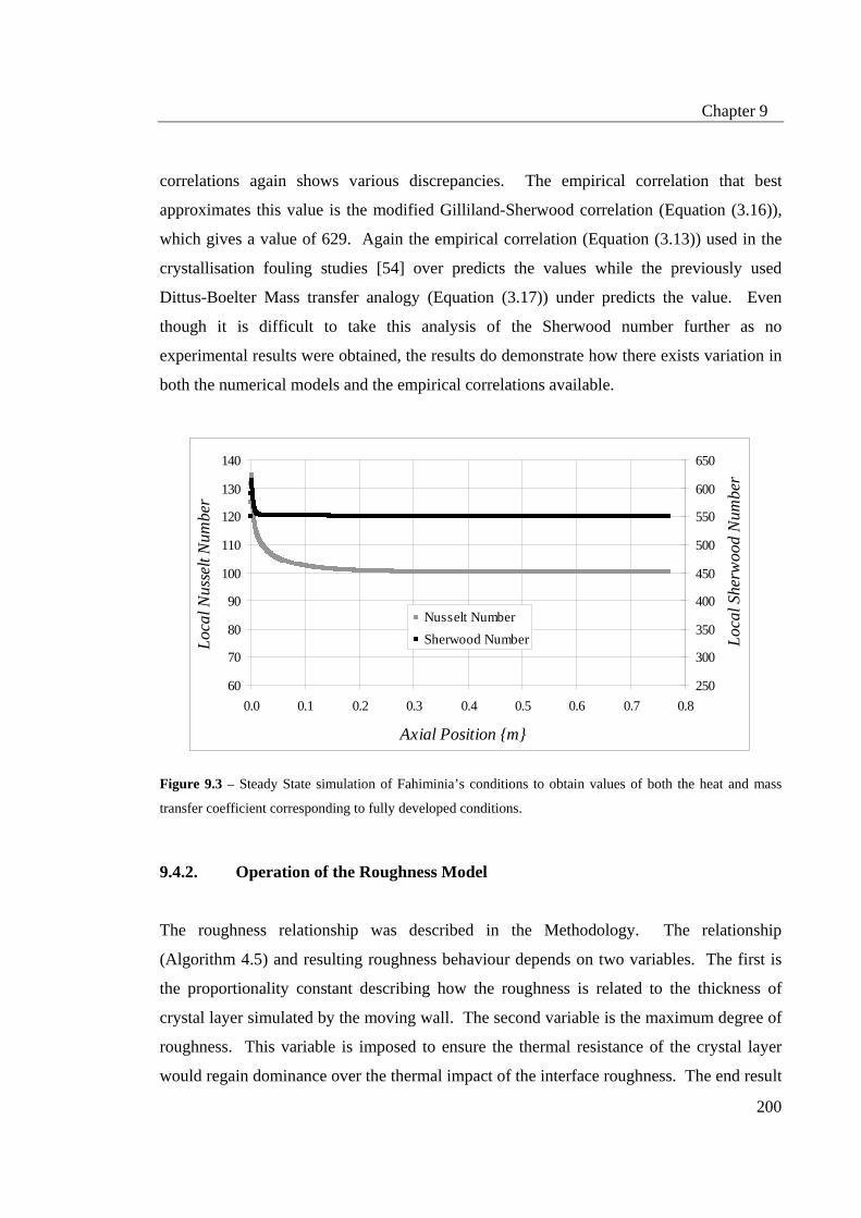
Chapter 9

200

correlations again shows various discrepancies. The empirical correlation that best

approximates this value is the modified Gilliland-Sherwood correlation (Equation (3.16)),

which gives a value of 629. Again the empirical correlation (Equation (3.13)) used in the

crystallisation fouling studies [54] over predicts the values while the previously used

Dittus-Boelter Mass transfer analogy (Equation (3.17)) under predicts the value. Even

though it is difficult to take this analysis of the Sherwood number further as no

experimental results were obtained, the results do demonstrate how there exists variation in

both the numerical models and the empirical correlations available.

60

70

80

90

100

110

120

130

140

0.0 0.1 0.2 0.3 0.4 0.5 0.6 0.7 0.8

Axial Position m

Loca

l Nus

selt

Num

ber

250

300

350

400

450

500

550

600

650

Loca

l She

rwoo

d N

umbe

r

Nusselt NumberSherwood Number

Figure 9.3 – Steady State simulation of Fahiminia’s conditions to obtain values of both the heat and mass

transfer coefficient corresponding to fully developed conditions.

9.4.2. Operation of the Roughness Model

The roughness relationship was described in the Methodology. The relationship

(Algorithm 4.5) and resulting roughness behaviour depends on two variables. The first is

the proportionality constant describing how the roughness is related to the thickness of

crystal layer simulated by the moving wall. The second variable is the maximum degree of

roughness. This variable is imposed to ensure the thermal resistance of the crystal layer

would regain dominance over the thermal impact of the interface roughness. The end result

Chapter 9

201

is a relationship that has the roughness as an indirect function of time as the key variable,

fouling layer thickness, changes with time. Figure 9.4 presents some preliminary results of

how this relationship operates. The figure plots the three variables involved in specifying

the roughness wall boundary condition; the thickness of the crystal layer, the non-

dimensional roughness and the equivalent sand grain roughness height. In the figure the

roughness variables are related to the thickness of the crystal layer. All variables in this

part of the figure are increasing linearly but with the roughness variables increasing with a

greater rate. This is an observation of how the proportionality constant, which relates the

thickness to the roughness variable, works. Another feature within the figure is the

enforcement of the constant roughness value whilst the crystal layer grows and its thickness

continues to increase. These two aspects were the fundamental ideas in the conceptual

development of the roughness relationship. Lastly, it is interesting to compare the two

roughness parameters. The comparison highlights how the two variables interact with each

other and the growing crystal deposit. Through specifying the maximum roughness via the

non-dimensional value a constant level of roughness is maintained while the actual

roughness decreases. This decrease is related to the changing hydrodynamic conditions

imposed by the movement of the interface.

0.0E+00

2.0E-05

4.0E-05

6.0E-05

8.0E-05

1.0E-04

1.2E-04

0 10000 20000 30000 40000 50000 60000

Time Seconds

Hei

ght

m

0

3

6

9

12

15

18

k+

Fouling LayerRoughnessk+

Figure 9.4 – Operation of the roughness model, a plot of the changing fouling layer height, roughness height

and dimensionless roughness parameter over time at a given position along the heat transfer surface (z = 0.76

m).

Chapter 9

202

Evaluating the impact that the aspects described in Figure 9.4 have on the fouling resistance

is possible through analysing Figure 9.5. The thermal resistance data for the

proportionality constant of six (a = 6) in Figure 9.5 corresponds to the roughness behaviour

of Figure 9.4. Immediately, it is observed that inclusion of the developed roughness

relationship has resulted in the occurrence of a rough delay time. Thus, confirming that the

initial idea behind the roughness component and its relation to the thickness operates as

intended when incorporated into the fouling model. Another important point that can be

made regards the selection of a suitable proportionality constant, ‘a’. The figure compares

two values of the proportionality constant a value of 6 and a value of 1. The latter was

included to confirm the assumption that roughness is not equivalent to the value of the

thickness.

-0.05

0.00

0.05

0.10

0.15

0.20

0.25

0 10000 20000 30000 40000 50000 60000

Time Seconds

Foul

ing

Resis

tanc

e m

2 K/k

W

Roughness 15 - a = 6Roughness 15 - a = 1

Figure 9.5 – Impact on the roughness on the fouling resistance over time and a comparison of using different

linear proportionality constants in the roughness algorithm at a given position along the heat transfer surface

(z = 0.7600 m).

The final aspect in verifying the operation of the roughness relationship is the assessment of

the impact of the maximum value for the dimensionless roughness factor (k+max). Three

values of the appropriate maximum value for the dimensionless roughness factor (k+max)

were selected for this assessment. The values of these variables were selected such that

Chapter 9

203

they fall within the completely rough regime [21]. The significance is that the completely

rough regime is where the roughness element protrudes through the laminar sub-layer to

produce high levels of roughness. Figure 9.6 demonstrates the results of using these

different maximum values through showing the impact theses values have on fouling

resistance. From the figure it is observed that the fouling rate experienced within the

growth period varies for the different maximum values. The fouling rate is greatest for the

lowest value of roughness and decreases for the maximum values of roughness. This is to

be expected because an increase in surface roughness is known to reduce the resistance to

heat transfer causing the surface temperature to drop. Higher temperatures result in

increased rates of crystallisation and hence, greater fouling rates. Turning the attention to

the induced roughness delay period it is apparent that the maximum value of roughness has

two effects. The first being the duration of the roughness delay time. The length of the

delay time appears to increase with increasing maximum roughness value. Again, this is

assumed to be related to the impact roughness has on crystal growth through temperature

but more detailed analysis will be conducted in the remaining sections. The second and

more interesting observation relates to the value of the minimum resistance. In Figure 9.6,

the minimum fouling resistance experienced varies from the lowest to the median value but

is identical when the median is compared to the highest. Without a more detailed

examination of the CFD solutions, it is a difficult to hypothesize as to why the minimum

fouling resistance is the same in these two cases making selection of the most suitable

upper limit difficult.

Chapter 9

204

-0.05

0.00

0.05

0.10

0.15

0.20

0.25

0 10000 20000 30000 40000 50000 60000

Time Seconds

Foul

ing

Resis

tanc

e m

2 K/k

W

Roughness 45Roughness 30Roughness 15

Figure 9.6 – A comparison of the impact that different maximum roughness values have on the characteristics

of an induced roughness delay period at the position corresponding to thermocouple 10 (z = 0.7600 m).

Figure 9.7 provides a detailed examination of the fouling resistance and is included to

evaluate the characteristic observed in Figure 9.6 regarding the minimum fouling

resistance. It plots the behavior of the non-dimensional roughness together with the fouling

resistance against time. Despite the data in Figure 9.6 belonging to a different axial

position, the same minimum characteristic is observed. It appears that increasing the

maximum value for the roughness beyond a certain magnitude has no impact on the

minimum value of the fouling resistance. Comparison of the two variables at the time that

minimum value occurs reveals that the minimum fouling resistance is surpassed before the

maximum roughness is attained. This confirms that the minimum fouling resistance indeed

has some kind of limit. The reason for this becomes apparent when the only factor that

could cause the increase in fouling resistance, producing the minimum, is considered. In

reference to the equation defining the fouling resistance, the only variable that could cause

the increase is the thickness of the fouling layer. Obviously the time taken for the fouling

thickness to have a noticeable impact of the fouling resistance, when also considering

roughness, is greater than that taken for the roughness to reach its maximum value. Hence,

for the case of a 45 level of roughness, the rate at which the fouling layer grows is quicker

Chapter 9

205

than the time taken for the roughness to reach its maximum. In both cases the rate depends

on the crystal growth, which is defined by the kinetics of surface crystallisation.

0

10

20

30

40

50

60

0 10000 20000 30000 40000 50000 60000

Time Seconds

k+

-0.05

0.00

0.05

0.10

0.15

0.20

0.25

Foul

ing

Resis

tanc

e m

2 K/k

Wk+

Fouling Resistance

Figure 9.7 – Comparing the temporal variation of fouling resistance with the corresponding roughness

relationship, which has a maximum non-dimensional roughness value of 45. The data was obtained at the

axial position corresponding to thermocouple 6 (z = 0.620 m).

This section described how the roughness relationship operates. The selection of the most

suitable maximum roughness value was made difficult by the occurrence of the minimum

fouling resistance that appeared independent of the maximum roughness value beyond a

certain value. Added to this problem, the experimental results did not provide any

information to justify the selection of one variable over another. Additional information is

required to more accurately evaluate the roughness relationship. The variable that would

provide most assistance is that of the behaviour of the overall pressure drop over time.

Most investigations that consider roughness examine the impact it has on the friction factor,

which is evaluated via the estimation of the overall pressure drop. Figure 9.8 is included to

emphasise this point and it compares the changing pressure drop for each case presented in

Figure 9.7 with that for the case where roughness is not considered. From Figure 9.8 it is

obvious that the inclusion of roughness imposes a drastic change in the pressure drop. If

Chapter 9

206

data could be obtain for pressure drop then a more sound value of the maximum roughness

variable could be ascertained.

0

500

1000

1500

2000

2500

3000

3500

0 10000 20000 30000 40000 50000 60000 70000 80000

Time Seconds

Pres

sure

Dro

p P

a

Roughness 45Roughness 30Roughness 15No Roughness

Figure 9.8 – The temporal change in the pressure drop experienced using different values for the maximum

roughness compared with the pressure drop experienced when roughness is not considered.

9.4.3. Use of the Roughness Relationship in the Numerical Fouling Model

9.4.3.1. The Operating Parameters

In this chapter the operation of the moving wall is similar to the previous. Observation of

the changing position of the solid-liquid interface shows how the propagation of the

nucleation front is simulated. Also, the comparison between the interface heat flux and the

interface position demonstrates how the wall boundary conditions operate. The difference

between the current chapter and the previous is the inclusions of roughness. Therefore this

section is devoted to highlight how the roughness influences and interacts with the

operating parameters.

Figure 9.9 plots the normal shear stress at the solid-liquid interface as calculated using the

scalable wall function approach. The plot is indicative of the hydrodynamic behavior

caused by both the movement of the interface and the impact it has on roughness. The

Chapter 9

207

shear maintains a constant value until the conclusion of the nucleation period. The initial

movement of the solid-liquid interface coincides with the increase of the roughness, which

depends on the solid-liquid interface position. Such an increase in the level of roughness,

towards its maximum value, causes a rapid increase in shear stress. The significance of

which is realized when compared to the behavior of the shear stress after the maximum

roughness value has been attained. Comparing the shear stress in Figure 9.9 with the

changing roughness in Figure 9.7 demonstrates that the rate at increase experienced by the

shear stress is more gradual once the maximum roughness value is reached. Within this

period it is only the movement of the interface surface that affects further change in the

hydrodynamics. Hence, the roughness induced by the growth of the crystal layer has a

significant impact on the hydrodynamics at the local positions along the solid-liquid

interface by increase the shear stress, which implies that there is a reduction in the

boundary layer thickness. An observed drop in the thickness of a boundary layer is

interpreted to mean that there is also a decrease in the resistance to transport and,

consequently, an increase in transport of species toward the solid-liquid interface. Finally,

the changing hydrodynamics in Figure 9.9 indicated that no longer is the flow fully

developed above the simulated crystal deposit in this two dimensional channel.

0123456789

10

0 20000 40000 60000 80000 100000

Time Seconds

Inte

rface

She

ar S

tress

Pa

Figure 9.9 – The impact of roughness on the temporal behaviour of shear stress at the solid-liquid interface

for the axial position corresponding to Thermocouple 6 (z = 0.620 m).

Chapter 9

208

The thermal properties have been established as having a dominant impact on the fouling

phenomenon and the resulting curves. This is still the case with the inclusion of roughness.

Analysis of the thermal properties assists in explaining how roughness causes both a

reduction in the fouling rate and the occurrence of the delay time. Figure 9.2 displayed the

initial distribution of temperature along the solid-liquid interface. Once the nucleation time

is surpassed the temperature distribution experiences considerable change. Figure 9.10 is a

plot of the temporal behaviour of the temperature distribution at a given local position.

There are three distinct characteristics in Figure 9.10, which correspond to the various

stages of surface roughness. The first is the aforementioned nucleation period where the

interface temperature maintains a constant value. Following this the temperature goes

through a rapid and significant decrease over a relative short time period. When compared

to Figure 9.7, this rapid drop in surface temperature coincides with the development of the

roughness and the commencement of the roughness delay time. Once the maximum

roughness is reached the temperature decrease becomes more gradual. This final

characteristic is maintained throughout the growth period and the rate of the growth period

experienced in Figure 9.7 is linear. Hence, despite a gradual temperature decrease, a linear

fouling rate is maintained. It would be interesting to test if the linear fouling rate is

maintained for a longer simulation time.

Chapter 9

209

346

348

350

352

354

356

358

0 20000 40000 60000 80000 100000

Time Seconds

Inte

rface

Tem

pera

ture

K

1.45

1.50

1.55

1.60

1.65

1.70

1.75

Inte

rface

Sup

ersa

tura

tionTemperature

Supersaturation

Figure 9.10 – The impact of roughness on the temporal behaviour of temperature and supersaturation at the

solid-liquid interface for the axial position corresponding to Thermocouple 6.

Another thermal variable that experiences considerable changes with the consideration of

roughness and influences the temporal behavior of the fouling resistance is the heat transfer

coefficient. Figure 9.11 is a plot of the local heat transfer coefficient and the thickness of

the deposited crystal layer against time. These are the two variables involved in the

calculation of the fouling resistance. The figure shows that the period where the local heat

transfer coefficient experiences a rapid increase is the same as that where the surface

roughness moves towards it maximum value (Figure 9.7). The roughness causes this

change in the local heat transfer coefficient, which is indicative of a reduction in the

resistance to heat transfer at the solid-liquid interface. It is similar to how the roughness

has impacted on the hydrodynamic behaviour, increasing the level or turbulence and

reducing the thickness of the boundary layer. These changes also have a significant

influence on the fouling resistance and induce the commencement of the roughness delay

period (Figure 9.7). Since the thickness of the fouled layer is minimal, the drastic decrease

in the thermal resistance causes the fouling resistance to obtain a negative value. This

behavior persists for a period of time until the thickness of the fouled layer (Figure 9.11)

causes its thermal resistance to balance the increased heat transfer. Eventually, the thermal

resistance of the fouled layer, which is proportional to its thickness, becomes more

Chapter 9

210

dominant than the reduction in heat transfer resistance caused by the roughness and causes

the fouling resistance to move into positive values. This method of operation, a balance

between the two resistances imposed by the use of a maximum fouling value was the

intention of the initial development of the roughness model. Such phenomenon has been

described in literature [22] where the occurrence of roughness has increased the turbulence

resulting in the roughness delay time.

0

2000

4000

6000

8000

10000

12000

14000

16000

0 20000 40000 60000 80000 100000

Time Seconds

Hea

t Tra

nsfe

r Coe

ffici

ent

W/m

2 K

0.0000

0.0001

0.0002

0.0003

0.0004

0.0005

0.0006

0.0007

0.0008

Foul

ed L

ayer

Thi

ckne

ss m

Heat Transfer CoefficientThickness

Figure 9.11 – Comparison of the changing thickness of the fouling layer and the impact of roughness on the

temporal behaviour of the local heat transfer coefficient at the solid-liquid interface for the axial position

corresponding to Thermocouple 6.

Roughness also has a noticeable impact on the interface supersaturation and the mass

transfer behavior. Figure 9.10 also plots the temporal variation in the supersaturation at the

solid-liquid interface. When compared to the corresponding plot from the previous chapter,

the most significance difference is the short but sudden increase in the supersaturation after

its initial drop. Following on from the previous analysis, this sudden increase is assumed to

be the influence of the surface roughness. There is no doubt that there surface roughness

impacts the resistance to mass transfer resistance in a similar way to the impact it had on

both the hydrodynamic and thermal boundary layers. Hence, the sudden rise in increase is

related to both an increase in the saturation concentration, induced by the drop in

Chapter 9

211

temperature, and a build up of concentration at the interface. Figure 9.12 is a plot of the

mass transfer coefficient and confirms that the sudden increase in roughness has caused a

similarly sudden drop in the resistance to mass transfer. It is concluded from this analysis

that the inclusion of roughness has promoted the transport of species towards the interface.

Finally, once the maximum roughness value has been achieved the supersaturation

experiences a steady increase, which is continued for the remainder of the simulation. An

increase in the supersaturation at the wall would increase the crystallisation flux but it

affects seem negligible as the corresponding fouling rate is a constant value through this

period (Figure 9.7).

0.00E+00

2.00E-05

4.00E-05

6.00E-05

8.00E-05

1.00E-04

1.20E-04

0 20000 40000 60000 80000 100000

Time Seconds

Mas

s Tr

ansf

er C

oeffi

cien

t m

/s

Figure 9.12 – The temporal behaviour of the local mass transfer coefficient at the solid-liquid interface for

the axial position corresponding to Thermocouple 6.

In this section the impact that the occurrence of roughness has on the various parameters

was apparent. However, it is worth acknowledging how that roughness value was

calculated. The uniqueness of the developed roughness relationship was that the degree of

roughness within the roughness delay period depended on the thickness of the simulate

crystal layer (Figure 9.11). The thickness is a variable whose values rely on those same

variables that were impacted by the development of a roughness towards a maximum value.

Chapter 9

212

Hence, the analysis provides an insight into how the key parameters and the thickness of

the fouled layer interact to produce the resulting phenomenon.

9.4.3.2. The Fouling Resistances

Figure 9.7 previewed the impact the developed roughness model has on the fouling

resistance. Figure 9.13 is included to gain a full appreciation of its influence. Figure 9.13,

which compare the solution for a smooth case and the roughness scenario. The comparison

demonstrates that the consideration of roughness impacts on each fouling process. The

nucleation time is lengthened as the nominal roughness of the geometry causes a slight

decrease in surface temperature, which translates to a slight increase in the induction time

(see classical nucleation equation). As previously discussed, the inclusion of the roughness

induced by the growing crystal layer results in the occurrence of the delay time. Lastly, the

inclusion of roughness causes a lower local fouling rate within the growth period. This

decrease is attributed to the previously observed sudden drop in the interface temperature.

The temperature drop was brought about by the roughness induced by the growth of the

fouling. Hence, the occurrence of fouling combined by the association of a level of

roughness has brought about a decrease in fouling rate relative to the conditions

experienced when no roughness was considered. In part, this is an observation of a process

referred to as auto-retardation, the formation of the deposit acting to inhibit the rate of

deposition [20]. However, in full, auto-retardation refers to the sustained decrease in the

fouling rate imposed by the reduction in the interface temperature. The observation of the

operating parameters showed there was a decrease in the interface temperature but the

linear fouling rate was maintained. Perhaps the interface temperature needs to experience a

larger variation within the growth period than it does in Figure 9.10 for a decreasing fouling

rate to be observed.

Chapter 9

213

-0.05

0.00

0.05

0.10

0.15

0.20

0.25

0.30

0.35

0.40

0 20000 40000 60000 80000 100000Time Seconds

Foul

ing

Resis

tanc

e m

2 K/k

W

No RoughnessRoughness 45

Figure 9.13 – Comparing the temporal variation of fouling resistance for the case of roughness and for the

case where roughness is not considered for the axial position corresponding to Thermocouple 10.

Figure 9.14 shows how these observed characteristics in the fouling resistance is present for

the curves at along the solid-liquid interface. These figures show that at different positions

the nucleation time is greater and the fouling rate is lower farther from the inlet. The

temperature at the positions in the figure is highest at that closest to the outlet during the

respective periods of nucleation and growth. As previously shown it is within the

roughness delay period the temperatures experience the most considerable change. From

Figure 9.14 it is difficult to differentiate between the behaviour within this period at each

position. Numerical analysis in the form of Table 9.1 shows that there is a trend in the

characteristics of the roughness delay time. Firstly, the length of the roughness delay time

is lowest closest to the outlet where the initial temperature is greatest. A similar

observation that associated shorter roughness delay times with an increased interface

temperature was made by Bansal [22] as well as from the experimental result of Fahiminia

[59]. However, Bansal’s statement was based on the overall fouling curves but these show

that idea hold when comparing the local fouling behaviour. The second characteristic

related to the minimum fouling resistance with the lowest experienced at the thermocouple

with the highest temperature, that closest to the outlet. Again one would relate this to the

rate’s dependency on temperature. It is difficult to ascertain a trend for this characteristic

Chapter 9

214

from the experimental result of Fahiminia [59] that would either confirm or repute these

numerical results. In addition, the closeness of the values in Table 9.1 makes it difficult to

draw any significant conclusions. Even though, the interface temperature does appear to be

the most influential parameter.

-0.05

0.00

0.05

0.10

0.15

0.20

0.25

0.30

0.35

0.40

0 20000 40000 60000 80000 100000

Time Seconds

Foul

ing

Resis

tanc

e m

2 K/k

W

Thermocouple 6Thermocouple 8Thermocouple 10

Figure 9.14 – The temporal variation of the fouling resistance at axial positions along the solid-liquid

interface position corresponding to thermocouples 6, 8 and 10 in the experimental set-up.

Axial Position Roughness

Delay Time Rf,min

Thermocouple

[m] [hr] [m2K/kW]

6 0.62 2.17 -0.0172

8 0.69 2.10 -0.0175

10 0.76 2.04 -0.0177

Table 9.1 – Numerical assessment of the fouling phenomena considering roughness using CFX-5.7

9.4.4. Validation of The Numerical Results

The purpose of this investigation was to include all the fouling processes observed

experimentally [59] in an effort to improve the numerical approximation of the fouling

Chapter 9

215

rates. In each of the fouling curves from the experiment [59] there occurred a nucleation

period and a roughness delay period. At those closer to the outlet there was also a growth

period with a linear fouling rate. The developed roughness relationship allows these three

processes to be duplicated in the numerical model with the results presented in Figure 9.14.

In Table 9.2, the values of the fouling rate for the roughness case indicates that the

roughness improves the numerical estimates for the fouling rates. A comparison of results

using CFX-5.7 demonstrates that the consideration of roughness improves the fouling rate

estimate calculated for smooth conditions by approximately 13%. However, there is a

difference of about 40 % between the numerical and experimental results. Acknowledging

that a maximum roughness of 45 is considerably large reinforces the significance of this.

Therefore, whilst including the impact that the growing layer has on roughness with the

other processes there still is a significant difference in the estimated value for the fouling

rate.

Experimental

Value CFX-4.3

CFX-5.7

Smooth

CFX-5.7

Roughness Thermocouple

[m2K/kJ] [m2K/kJ] [m2K/kJ] [m2K/kJ]

6 * 7.64×10-6 7.41×10-6 6.38×10-6

8 4.27×10-6 7.86×10-6 7.65×10-6 6.62×10-6

10 4.85×10-6 8.06×10-6 7.88×10-6 6.86×10-6

Table 9.2 – Comparison of fouling rates obtained from CFX-4.3, CFX-5.7 for no roughness and CFX-5.7 for

roughness with that from the experimental data. The * denotes an inability to extract a reliable value for

fouling rate as the experimental data plot ends shortly after the end of the roughness delay time.

The secondary part of the validation is to compare the resulting wall temperature. The wall

temperature in Figure 9.15 was calculated based on the corresponding interface

temperature, the heat flux and the thermal resistance of the fouled layer. The thermal

resistance is a function of the thickness of the fouled layer and its assumed thermal

conductivity. Only the final of the wall temperature distribution is available from

experimental data [59] for a comparison. The final value at the corresponding

thermocouple is significantly less than that in Figure 9.15. The behaviour in Figure 9.15

Chapter 9

216

and the decrease experienced within the roughness delay period is confirmed by comparing

the final temperatures at the positions along the interface that are still experiencing the

roughness delay period at the termination of the experiment.

350

360

370

380

390

400

410

420

0 20000 40000 60000 80000 100000

Time Seconds

Wal

l Tem

pera

ture

K

Figure 9.15 – A plot of the variation of the wall temperature with time the axial position corresponding to

position 0.620 m (Thermocouple 6).

Completion of the validation allows a closer examination of the reasons behind the

differences in the fouling rate to be elucidated. Comparisons of all the figures for the

numerical fouling results in this chapter and the previous chapter with the experimentally

data demonstrated that the time taken to reach the same level of fouling resistance was

much shorter in the numerical case. Furthermore, the assessment of the roughness

relationship indicated that an increase in maximum roughness would have no impact since

the minimum value of the fouling resistance is surpassed before the maximum roughness

value is achieved. The minimum values obtained numerically did not compare well with

the corresponding experimental values, which were much less. Finally, the observed value

of the final wall temperature thermocouple represented in Figure 9.15 was much larger than

that experienced experimentally. These parameters are functions of time and demonstrate

that the fouling phenomenon is occurring significantly faster in the numerical results than

the experimental. The most apparent explanation lies in the specification of the

Chapter 9

217

crystallisation kinetics for the surface reaction. The kinetic data was obtained from

literature [54] and utilized within the numerical model does not appear to match the given

experimental results [59].

It is worthwhile recalling the method used to evaluate the surface crystallisation kinetics

considering that they appear to be the key area influencing the over-prediction of the

fouling rates. The material section reviewed how Bohnet [54] experimentally evaluated

surface kinetics based on the empirical resistance based models and the overall fouling

resistance (Equation (3.12)). It was explained that the important role of the mass transfer

coefficient played in the assessment of the kinetics. The values used for the mass transfer

coefficient were derived from a selected Sherwood number correlation by Equation (3.13).

Previous analysis of the Sherwood number, in this chapter, showed that the Sherwood

numbers calculated numerically was considerably less than that calculated. Using the

temperature variation of mass transfer coefficient (Figure 9.12) the corresponding

Sherwood number can be calculated (Figure 9.16). Again, it is exhibited that the range of

Sherwood number experienced is considerably less than the value calculated for the same

conditions using Equation (3.13). Hence, it is possible that a difference between the mass

transfer coefficient from the simulations and the empirical correlation used in

Crystallisation studies could indirectly explain the over-prediction of the fouling rate.

Perhaps if the CFD models were used to revise the Sherwood correlations then a value of

the reaction rate constant could be established that would better predict the fouling rates.

However, the difficulty is that the numerical results of the Sherwood numbers vary

significantly for the different turbulent models.

Chapter 9

218

0

200

400

600

800

1000

0 20000 40000 60000 80000 100000

Time Seconds

Loca

l She

rwoo

d N

umbe

r

Figure 9.16 – The temporal behaviour of the Sherwood Number based on the mass transfer coefficient in

Figure 9.12.

9.5. Enhancement of the Roughness Model

The roughness model applied in this investigation was based on experimental observations.

It specified the degree of roughness to be dependant on the thickness of the crystal layer

and hence, modelled the roughness induced by the developing crystal layer. A plot of the

temporal variation in the fouling resistance demonstrated that this relationship produced a

roughness delay period, a phenomenon observed within the experimental results used for

validation. However, there exists a difference in the characteristics of the two types of data

for the roughness delay period. This final section compares the characteristics or shape of

the roughness delay period in both sets of data in an effort to establish possible areas where

the roughness model could be enhanced.

The roughness delay period in Figure 9.7 appears not to be symmetrical in form. This lack

of symmetry within the roughness delay period is also observed in the experimental fouling

curves (Figure 3.2). In the numerical results, the rate at which the fouling resistance

decreases towards its minimum value is greater than that at which it ascends from the

minimum. This form of the roughness delay period is not observed in the experimental

Chapter 9

219

fouling curves. In fact the form is actually opposite to the numerical results. Using the

knowledge gained from examining the numerical results it is possible to establish a reason

for this difference. In the numerical results, it is observed that the increasing roughness

corresponds to a decrease in temperature and a reduction in the crystallisation and, hence,

fouling rate. Based on this knowledge, the increase in the fouling rate observed in the

experimental results, from the minimum value of the fouling resistance, implies the

interface temperature has experienced an increase. Such an increase appears only possible

if there is a reduction experienced in the interface roughness, which causes the surface

temperature to increase.

In an effort to improve the roughness model, it is beneficial to evaluate possible reasons for

the implied reduction in surface roughness experienced experimentally following the

minimal value of the fouling resistance. This assumed change in roughness could relate to

the interaction between the crystal characteristics and the changing hydrodynamic forces at

the interface. For example, as the thickness of the crystal layer grows and the channel

narrows, the shear force experienced at the solid-liquid interface would increase. The

change in shear force at the interface is likely to affect the crystal characteristics including

its surface texture. In a previous investigation by Helalizadeh [14] into crystallisation

fouling, the texture of the crystal deposit was examined and quantified by defining its

fractal dimension. This concept of interface texture has also appeared in work by Scaggs

[79] that attempts to characterise surface roughness. Scaggs states how traditional

approaches to the roughness problem suffered from the omission of texture information.

The omission of texture overlooks cases where two surfaces with the same average

roughness height can have significantly different friction coefficients. An idea supported

by Tarada [80], who states that the gaps between roughness elements are important in the

characterization of surface roughness. The fractal dimension determined by Helalizadeh

[14] is a variable that represents this concept It is defined as the efficiency of an object to

take up space [62]. Another reason for the change in the surface texture of the crystal layer

surface is the occurrence of secondary nucleation would cause crystals to grow in gaps of

the crystal layer. Secondary nucleation is the nucleation which occurs on the crystal

deposits. This nucleation often occurs within the gaps of the deposit and, consequently has

Chapter 9

220

an impact on the texture of the deposit’s surface. By changing the texture of the surface

and this would impact on the roughness based on the idea suggested by Tarada [80].

These possibilities serve to demonstrate the complexity of modelling the surface roughness

at the crystal interface. It implies that there exist limitations by having just the equivalent

sand grain roughness to specify roughness. An alternate candidate is the ratio of the

apparent wall shear stress due to form drag on the roughness elements to the total wall

shear stress [35] although it is still a representation of roughness with a single variable.

Also, it is conceivable that a variable like the fractal dimension could be used to

characteristic the roughness. Tarada [80] suggested using a number of variables to give a

full description of the finite roughness elements. However this is restricted by the

capability of the turbulence model, which only uses the equivalent sand grain roughness to

quantify the roughness.

Chapter 10

221

10. Conclusions and Recommendations Equation Chapter 10 Section 1

10.1. Conclusions

This project demonstrated the usefulness of adopting the Computational Fluid Dynamics

(CFD) method in examining heat exchanger fouling and associated phenomena. The

project’s objective was to develop a model using CFD that would detail the fouling

common to crystalline streams. Once completed, the model would assist in furthering the

understanding of fouling as well as the intricate interactions of key operation of parameters

on a local scale. Model components were developed and assessed using a progressive

stage-wise strategy. The first stage examined the Eulerian approach to the occurrence of

calcium sulphate precipitation within the flow. It was revealed that the Eulerian modelling

approach was suitable for the aqueous phase but not for the precipitated particulate phase.

A revised Lagrangain approach for the particulate phase was adopted for the next stage of

evaluating the combined crystallisation and particulate mechanisms. This ability to change

approaches but to continual progress demonstrates the benefit of adopting a stage-wise

strategy in its ability to progressively assess the suitability of individually components.

These initial stages were conducted assuming steady state conditions. It allowed an

assessment of the operation and physical accuracy of the precipitation occurring both

within the flow and at the heat transfer surface. Another significant stage was the transition

from steady state to transient conditions. It would have been difficult to evaluate the

operation of all the individual model components using the transient case where the use of

the moving wall technique significantly increased the model’s complexity. This stage wise

development was accompanied by verification and validation techniques, which were

continually used to determine the adequacy of the model. These techniques detected the

suitability of the applied methods and identified areas requiring improvement. Another

benefit of employing this overall approach was the characteristics revealed in the analysis

of each stage that contribute to increasing the knowledge of fouling and associated

precipitation phenomena.

Chapter 10

222

The first stage in model development was the examination of calcium sulphate precipitation

in both laminar and turbulent flow. Precipitation occurs in saline streams where there is a

significant level of sparingly soluble salts. Based on a modified rate equation, the

governing transport equations for the aqueous species were altered to simulate their

consumption within the geometry. Extensive verification techniques showed how a

reaction rate equation and corresponding kinetic data from literature could be successfully

incorporated into the model. Further testing demonstrated how the kinetic value

incorporated into the model could be calculated from the actual numerical solutions. Use

of this precipitation model in both laminar and turbulent flow revealed some intriguing

characteristics relevant to the fouling phenomena. The findings inferred that velocity and

residence time distribution influences the behavior of the precipitation process. The

velocity and residence time distribution causes the emergence of a concentration gradient of

the aqueous species adjacent the wall. These induced concentration gradients could

conceivably cause species to diffuse towards the transfer surface and promote deposition by

the crystallisation mechanism at the surface. The alternate is that the increased

precipitation could result in the deposition via the particulate mechanism. A study of the

impact which operating conditions had on this precipitation behavior revealed that the

severity of these concentration gradient were influence by velocity, temperature and inlet

supersaturation. The difference in flow conditions was that in turbulent flow these

concentration gradients were confined to the sub layer where in the laminar flow the

gradients extend into the bulk. This ability of the CFD approach to effectively simulate

precipitation process has assisted in gaining improved understanding of velocity,

temperature, and concentration gradients affecting the fouling mechanisms.

The precipitation component of the model was utilized in chapter 6 to observe its behavior

in different geometries and to establish whether there existed a link between the observed

characteristics in these geometries. In attempting to establish a link the behavior was

compared based on three key hydrodynamic variables that are often used in the

characterization of the fouling phenomenon. The three key hydrodynamic variables are

velocity, shear stress and the Reynolds number. However, the effort to inter-relate the

precipitation behavior in rectangular slits to tubular geometries proved unsuccessful. It

Chapter 10

223

seemed that these hydrodynamic variables are not suitable measures of comparing the

results for different geometries. Results indicated that the geometry was the main factor

contributing to the observed difference in the precipitation and consequently concentration

gradients. In fact, the concentration gradients formed within the tubular geometry were

consistently greater than that for the rectangular slit. It would appear that, based on the

previously mentioned diffuse idea and its relation to the concentration gradients, the tubular

geometry would be more prone to possible crystallisation fouling and possible particulate

fouling.

The second stage involved continuing the precipitation concept from the previous chapter

with the consideration of both the crystallisation and particulate flux at the heat transfer

surface. This required altering the model to consider the occurrence of precipitation to both

within the bulk/boundary layer and at the wall, as part of the overall crystallisation

mechanism. Particulate fouling was also included as the emphasis of the investigation was

to assess the likelihood of composite fouling through validation even though the numerical

simulations were conducted at steady state. The most intriguing of this Eulerian-

Lagrangian model was its ability to convert the transport of a discrete particle to a value for

flux provided the particulate matter deposited. The resulting accumulated particulate flux

was distributed along the heat transfer surface.

The numerical solutions for the particulate and crystallisation flux were validated with

corresponding experimental thickness distributions to provide an insight into factors

determining the likelihood of the fouling mechanisms. The numerical results considered

the case where precipitation occurred within the bulk/boundary layer and the case where

precipitation only occurred at the surface. For laminar flow, the results comparison of the

two cases with the experimental results indicated that no precipitation occurred within the

bulk/boundary layer and crystallisation was the only fouling mechanism present. For the

turbulent case, the experimental results compared best with the case where precipitation

was occurring within the bulk/boundary layer and, thus, implying both mechanisms

occurred. Closer analysis of the flux distributions for the turbulent case proves the valuable

insight that this model could give into composite fouling. Firstly, the ability of modelling

Chapter 10

224

the individual flux mechanisms allowed the balance of mechanisms to be evaluated.

Secondly, it showed the ability to evaluate the dominant fouling mechanism, the particulate

mechanism in the turbulent case. Thirdly, the model showed how it was able to

differentiate between the precipitation within the bulk, boundary layer and that at the

surface. It revealed that the deposited particles were generated within the boundary layer

and not the bulk, emphasizing the importance of possessing the capability to assess the

interactions within the boundary layer. The detail used in making these assessments was

also applied to the local operating parameters and assisted in elucidating the most

influential parameter on a local scale. The supersaturation proved to be most influential

when precipitation was occurring within the bulk/boundary layer but in its absence the

surface temperature was the dominant variable. This type of analysis is another example of

the level of detail enable to be achieved when using CFD. The final point of significance in

this section relates to the impact the inclusion of the crystallisation flux had on the

emerging concentration gradients within the flow. The results portrayed that a higher

amount of crystallisation flux was achieved when precipitation was not occurring within the

flow despite the emergence of the aforementioned concentration gradients. It appears the

higher degree of supersaturation at the surface was the determining factor rather than the

diffusion of species induced by the emergence of the concentration gradients. Therefore,

the correct assessment would be that the occurrence of precipitation within the flow,

particularly the boundary layer, increase the likelihood of particulate fouling and reduces

the possible amount of crystallisation flux.

The following stage required the transition from the steady state scenario to considering

dynamic behavior of the deposition using transient simulations. The significance of this

stage was the development of various physical models and numerical methods to allow the

true dynamic nature of fouling to be reproduced. This involved using experimental results

to create a relationship describing the nucleation and a relationship to account for the effect

of the changing wall position on the local interface heat flux. Central to the operation of

this transient simulation was the adoption of the moving wall technique to simulate the

actual deposit growth. The impact that deposit growth had in terms of fouling was

observed through the calculation of the fouling resistance and monitoring its temporal

Chapter 10

225

variation. The resulting fouling curves were used to estimate numerical values for the

fouling rate. Validation with experimental work confirmed the successful reproduction of

the transient crystallisation fouling. It also demonstrated the CFD ability to satisfactorily

predict the fouling rates. Hence, the key objective of creating a predictive fouling model

was successfully achieved. Another key objective achieved was in the ability of the CFD

method employed to examine the behavior of operating parameters on a local scale over

time. The detail of the CFD method gave a new insight into the intricate interactions

occurring between key operating parameters on a local scale. The moving wall also

imposed a change on the local hydrodynamic behaviour. This changed caused a movement

and subsequent buildup of species adjacent the wall. Despite this continual build up of

species and increase in the local interface supersaturation the fouling rate maintained a

constant value, which is indicative of the dominant influence of the interface temperature.

The only concern with this numerical model was it’s over prediction of the experimentally

determined fouling rates. However, it was hard to make a comprehensive analysis to

explain the reasons for this over prediction without the inclusion of a roughness delay

period, which was present in the experimental results.

The final stage saw the inclusion of the impact that the depositing material had on the

roughness of the solid-liquid interface into the unsteady crystallisation model. This

interface roughness was included in an effort to allow a comprehensive analysis of the

difference observed between the numerical and experimental fouling rates. A validation of

the initial unsteady crystallisation model demonstrated the absence of a roughness delay

period. An innovative model was developed based on the concept that the roughness delay

period was a balance between the interaction of the local variables and the interface

roughness induced by the crystal deposit. Through successfully reproducing the roughness

delay period, the numerical results demonstrated precisely what had been observed

experimentally. The thermal resistance of the growing deposit eventually countered the

advantage that the interface roughness has on promoting heat transfer. This inclusion of

roughness provided further insight into the interaction of the developing deposit and the

local behavior of the operating parameters. At a local level, the occurrence of roughness

considerably increased the build up of the species adjacent the wall and at the same time

Chapter 10

226

caused a significant drop in the local temperature at the interface. Analysis of the predicted

fouling rates indicated that the behavior of the interface temperature was more influential

than the interface supersaturation because the predicted fouling rates dropped. Relative to

the case of the smooth wall, the predicted fouling rates dropped and the occurrence of local

roughness delay period was testimony to the successful operation of the roughness

relationship. However, the predicted fouling rates were still high compared with the

experimental results. As roughness has been modeled, a thorough analysis of possibilities

indicated that the used kinetic values from literature were most likely the significant factor

in the over-prediction of the fouling rates.

The completion of various stages continually provided evidence that CFD was a worthy

tool in modelling the intricate fouling processes. It was observed that the developed model

components operated satisfactorily at the intended conditions for comparison. However, in

various chapters the inability of the various components to operate for a broader range of

conditions was discussed. This was initially referred to in chapter 7 whilst examining the

operation of the derived physical models and the combined fouling mechanisms. The

objective was to examine the behavior of these mechanisms for a range of operating

conditions. However, it was discovered that there existed limitations in the operation of

key components in the developed CFD model. The most interesting point raised was the

implication that the kinetic data used within the crystallisation boundary conditions

operated only for a certain range of both thermal and supersaturation conditions. The

significance of these findings was questioned by the use of steady state conditions when

fouling is a dynamic phenomenon. However, similar issues were raised concerning the

kinetics in the remaining chapters investigating transient conditions. These issues surfaced

when the predicted fouling rate significantly over-predicted the experimental results even

though the impact of the interface roughness was considered. Ultimately, the same level of

fouling resistance was achieved numerically over a shorter time period than was observed

experimentally. Hence, for the second time within the investigation the kinetics of the

crystallisation boundary condition appeared to be a contributing factor in the problems

observed numerically. Both of these cases were revealed based on the same strategy of

validation. Early in the investigation this simple but comprehensive strategy of validation

Chapter 10

227

was devised. It consisted of separately validating the transport phenomena and the fouling

processes. Its importance to the study was revealed in the above assessment regarding the

appropriateness of the crystallisation boundary conditions and, in particular, the kinetic data

incorporated from the literature.

The application of the CFD method has proven to be beneficial in investigating various

aspects of fouling associated with crystalline streams. In both the literature review and the

materials section, the advantages of using the CFD method with its ability to provide detail

of the behaviour of key operating parameters on a local scale was emphasized. This aspect

was utilized in the analysis of the results for key operating variables at local level to

provide an insight into fouling. In addition, the commercial CFD model was successfully

modified with developed user subroutines to model the true transient nature of fouling. The

ability of the resulting CFD model to predict the temporal variation of fouling resistance

proves the numerical method is an effective alternative to the traditional experimental

approach.

10.2. Recommendations

The recommendations for further research cover two areas. The first continues from the

final point in the conclusion and focuses on the need to obtain suitable experimental data.

Suitable experimental data would assist in improving key components of the current model

and allow its use over a wider range of operating conditions. Once this improvement has

been achieved then the model can be extended further to complete the modelling, which is

the second area recommended to be investigated in further research. Ultimately, the goal

should be to complete a transient CFD model capable of operating over a range of

conditions that predicts composite fouling.

An important part of developing a model of any phenomena is to ensure it reliably operates

over wider range of boundary conditions. The analysis of the CFD model developed in this

research indicates that additional work is required to enable the use of a wider range of

boundary conditions. Additional work should initially focus on further evaluating the

Chapter 10

228

kinetics used in the boundary conditions. It was implied that the mass transfer coefficient

could perhaps be the determining factor. Given the right experimental information this

could be established. More suitable crystallisation kinetic data could have been elucidated

from the results used for validation if more detail was provided. Hence, a co-operation is

necessary between the experimental and numerical investigations with the emphasis on

making sure a complete set of data required for validation is obtained. Another example,

which encapsulates this idea, relates to the nucleation model. The nucleation relationship

in this thesis represented only a portion of the actual work conducted on the nucleation.

Most of the work involved attempting to developed a universal relationship based on

various investigations mentioned in the literature review. However, the objective was

hampered by the lack of suitable data available and it was not until a complete set of data

become available that a nucleation relationship could be developed. In this instance the

complete data was in the form of a local distribution of both induction time and

temperature, which facilitated the derivation of a suitable empirical model. The depth of

information in this set of data was not enough to generalize the model and evaluate the

values of the key thermodynamic aspects defined in the classical nucleation theory,

particularly on a local level. Similar issues were raised in the discussions regarding the

accurate assessment of the roughness delay period and the need for information about the

temporal behavior of the pressure drop. The most sensible solution is for the parallel

running of the experimental and numerical investigations. To run the experimental and

numerical investigations in parallel is the most desirable scenario when conducting any

type of CFD investigation. However, it is difficult to do so when the additional subroutines

required take a considerable amount of time to both develop and verify.

Once a complete set of experimental data is obtained and the scope of the existing CFD

model broadened then it can be extended. The most obvious extension is the completion of

an unsteady model of composite fouling. This would involve revising some of the existing

physical models like nucleation, which is known to vary in the presence of particulate

matter. Also, the occurrence of composite fouling is known to significantly impact the

kinetic data and, hence, the corresponding boundary conditions would need to be re-

evaluated. The drawback of pursuing this unsteady simulation of composite fouling would

Chapter 10

229

be the time required following each time step to obtain the particulate flux by running the

Lagrangian modelling component. Such a simulation would take longer than running a

corresponding experimental run. An alternative is to run a number of simulations to obtain

a table of reference covering the key variables, like the balance of mechanisms, over a

range of operating conditions. This seems reasonable as it coincides with the next step that

involves investigating the effect of operating parameters to determine the optimal operating

condition for minimizing the occurrence of fouling. Other key areas include considering

removal and, thus, considering the net fouling rate rather than just the deposition. Another

extension would be transferring the model from 2D to 3D. However, the initial focus

should be on ensuring that the model developed in this project operates for the intended

processes over a range of operating conditions. By broadening the scope of the model

components and ensuring its operation then work could commence on its extension.

References

230

References 1. Ritter, R.B., Crystalline Fouling Studies. Transactions of the ASME, 1983. 105: p.

374-378.

2. Karabelas, A.J., Scale formation in tubular heat exchangers—research priorities.

International Journal of Thermal Science, 2002. 41: p. 682–692.

3. Taberok, J., Ritter, R. B., Palen J. W., Heat Transfer; Fouling: The Major

Unresolved Problem in Heat Transfer. Chemical Engineering Progress, 1972.

68(2): p. 59-67.

4. Epstein, N., Thinking about Heat Transfer Fouling: A 5x5 matrix. Heat Transfer

Engineering, 1983. 4(1): p. 43-56.

5. Brahim, F., Ausgustin, W., Bohnet, M., Numerical simulation of the fouling

process. International Journal of Thermal Sciences, 2003. 42: p. 323-334.

6. Mwaba, M.G., Analysis of Heat Exchanger Fouling in Cane Sugar Industry. 2003,

Technische Universiteit Eindhoven: Eindhoven. p. 132.

7. Kho, T.C.S., Effect of Flow Distribution on Scale Formation in Plate and Frame

Heat Exchangers, in Chemical and Process Engineering. 1998, Surrey: Guildford.

p. 292.

8. Bailey, K., Optimise Heat Exchanger Operations By Minimising Fouling.

Hydrocarbon Processing, 1999(July): p. 113-127.

9. Mukherjee, R., Conquer heat exchanger fouling. Hydrocarbon Processing, 1996: p.

121-127.

10. Epstein, N. Fouling in Heat Exchangers. in Proceedings of the 2nd International

Conference Heat Transfer. 1978.

11. Kho, T., Muller-Steinhagen, H., An experimental and numerical investigation of

heat transfer fouling and fluid flow in flat plate heat exchangers. Trans IChemE,

1999. Part A, 77: p. 124-130.

12. Sinnott, R.K., Coulson, J. M., Richardson, J. F., Coulson & Richardson's Chemical

Engineering. 2 ed. Vol. 6. 1996, Oxford: Butterworth-Heinemann.

13. Bott, T.R., Fouling of Heat Exchangers. 1995: ELSEVIER science B.V.

14. Helalizadeh, A., Muller-Steinhagen, H., Jamialahmadi, M., Mixed salt

crystallisation fouling. Chemical Engineering and Processing, 2000. 39: p. 29-43.

References

231

15. Levine, S., Bowen, B., Epstein, N., Fine Particle Deposition in Smooth Parallel-

Plate Channels. Journal of Colloidal and Interface Science, 1976. 54(3): p. 375-390.

16. Bowen, B., Epstein, N., Fine Particle Deposition in Smooth Parallel-Plate

Channels. Journal of Colloidal and Interface Science, 1979. 2(1): p. 81-97.

17. Schreier, P.J.R., Heat Exchanger Fouling: a model study of Laboratory Data.

Chemical Engineering Science, 1995. 55(8): p. 1311-1321.

18. Grijspeerdt, K., Hazarika, B., Vucinic, D., Application of computation fluid

dynamics to model the hydrodynamics of plate heat exchangers for milk processing.

Journal of Food Engineering, 2003. 57: p. 237-242.

19. Muller-Steinhagen, H., Zhao, Q., Helali-Zadeh, A., Xiao-Guang Ren, The effect

surface properties of CaSO4 scale formation during convective heat transfer and

subcooled flow boiling. The Canadian Journal of Chemical Engineering, 2000.

78(February): p. 12-20.

20. Bansal, B., Muller-Steinhagen, H., Chen, X. D., Performance of plate heat

exchangers during calcium sulphate fouling - investigation with an in-line filter.

Chemical Engineering and Processing, 2000. 39(6): p. 507-519.

21. Schlichting, H., Boundary Layer Theory. 6th ed. 1968, New York: McGraw-Hill

Book Co., Inc.

22. Bansal, B., Muller-Steinhagen, H., Crsytallization Fouling in Plate Heat

Exchangers. Transactions of the A.S.M.E., 1993. 115(August): p. 584-591.

23. Sheikholeslami, R., Calcium Sulfate Fouling - Precipitation or Particulate; A

Proposed Composite Model. Heat Transfer Engineering J., 2000. 21(2): p. 24-33.

24. Kostoglou, M., Andritsos, N., Karabelas, A. J., Flow of supersaturated solutions in

pipes. Modelling bulk precipitation and scale formation. Chemical Engineering

Communications, 1995. 133: p. 107-133.

25. Amjad, Z., Calcium Sulfate Dihydrate (Gypsum) Scale Formation on Heat

Exchanger Surface: The Influence of Scale Inhibitors. Journal of Colloid and

Interface Science, 1988. 132(2).

26. Sheikholeslami, R., Nucleation and Kinetics of Mixed Salts in Scaling. AIChE

Journal, 2003. 49(January): p. 194-202.

References

232

27. Hasson, D., Zahavi, J., Mechanism of Calcium Sulfate Deposit on Heat-Transfer

Surfaces. I&EC Fundamentals, 1970. 9(1): p. 1-10.

28. Bramson, D., Hasson, D., Semiat, R., The roles of gas bubbling, wall crystallisation

and particulate deposition in CaSO4 scale formation. Desalination, 1995. 100: p.

105-113.

29. Taberok, J., Ritter, R. B., Palen J. W., Heat Transfer: Part 2; Predictive Methods

for Fouling Behaviour. Chemical Engineering Progress, 1972. 68(7): p. 69-78.

30. Forster, M., Bohnet, M., Influence of the interfacial free energy crystal/heat transfer

surface on the induction period during fouling. International Journal of Thermal

Science, 1999. 98(11): p. 944-954.

31. Forster, M., Augustin, W., Bohnet, M., Influence of the adhesion force crystal/heat

exchanger surface on fouling mitigation. Chemical Engineering and Processing,

1999. 38: p. 499-461.

32. Pigott, R.J.S., The Flow of Fluids in Closed Conduits. Mechanical Engineering,

1933(August): p. 497.

33. Moody, L.F., Princeton, N. J., Friction Factors for Pipe Flow. Transactions of the

A.S.M.E., 1944(November): p. 671-684.

34. Fred Farshad, H.R., James Garber, New developments in surface roughness

measurements, characterization, and modelling fluid flow in pipe. Journal of

Petroleum Science and Engineering, 2001. 29: p. 139-150.

35. Scaggs, W.F., Taylor, R. P., Coleman H. W., Measurement and Prediction of Rough

Wall Effects on Friction Factor - Uniform Roughness Results. Journal of Fluids

Engineering, 1988. 110(December): p. 385-391.

36. Parkins, W.E., Paper 9. 1961, Atomic Energy of Canada Ltd.: Chalk River,

Ontario.

37. Watkinson, A.P., Epstein, N. Paper HE 1.6. in Proc. 4th IHTC. 1971: Elsevier.

38. Beal, S.K. Paper No. 76-C. in 65th Annual Meeting AIChE. 1972. New York.

39. Beal, S.K., Nuclear Science and Engineering, 1970. 40(1).

40. Epstein, N., Particulate Fouling of Heat Transfer Surfaces: Mechanisms and

Models. Fouling Science and Technology, 1988: p. 143-164.

References

233

41. Ruckstein, E., Prieve, D. C., Journal of Chemical Society Faraday II, 1973. 69: p.

1522.

42. Chang You-Im, W.J.-J., Particle Deposition Behaviour Simulated by the Stochastic

Method. Journal of Petroleum Science and Engineering, 1999: p. 189-203.

43. Wiesner, M.R., Morphology of Particle Deposits. Journal of Environmental

Engineering, 1999: p. 1124-1132.

44. Pomeau, Y., Resibois, P., Time dependant correlations functions and mode-mode

coupling theories. Physics Reports, 1975. 19(2): p. 63-139.

45. Lightfoot, E.N., Building Randomness. The Chemical Engineer, 1990(July 12th): p.

18-19.

46. Lightfoot, E.N., Bird, R. B, Stewart, W. E., Transport Phenomena. 1960: John

Wiley & Sons.

47. Walker, P., Sheikholeslami, R., Assessment of the effect of velocity and residence

time in CaSO4 precipitation flow reaction. Chemical Engineering Science, 2003.

58(16): p. 3807-3816.

48. Mori, H., Nakamura, M., Toyama, S., Crystallisation Fouling of Calcium Sulfate

Dihydrate on Heat Transfer Surfaces. Journal of Chemical Engineering of Japan,

1996. 29(1): p. 166-173.

49. Versteeg, H., Malalasekera, W., An introduction to Computational Fluid Dynamics.

1995, Harlow: Pearson Education Limited.

50. Orszag, S.A., Staroslefky, I, CFD: Progress and Problems. Computer Physics

Communications, 2000. 127: p. 165-171.

51. Roache, P.J., Perspective: A method for uniform reporting of grid refinement

studies. Journal of Fluids Engineering, 1994. 116(September): p. 405-413.

52. Incropera, F.P., DeWitt, D. P., Fundamentals of Heat and Mass Transfer. 1996:

John Wiley & Sons.

53. Liu, S., Nanacollas, G. H., The kinetics growth of crystal calcium sulphate

dihydrate. Journal of Crystal Growth, 1970. 6: p. 281-289.

54. Bohnet, M., Fouling of Heat Transfer Surfaces. Chemical Engineering Technology,

1987. 10: p. 113-125.

References

234

55. Krause, S., Fouling of heat transfer surface by crystallisation and sedimentation.

International Chemical Engineering, 1993. 33(3): p. 355-401.

56. Hines, A.L., Maddox, R. N., Mass Transfer Fundamentals and Applications. 1985,

New Jersey: PTR Prentice-Hall Incorporated.

57. Valiambas, S., Andritsos, N., Karabelas, A. J., An Assessment of data and

Predictive Tools For Cooling Water Fouling of Heat Exchangers, in Energy

Efficiency in Process Technology, P.A. Pilavachi, Editor. 1993.

58. Chong, T., Comparison of CaSO4 experimental fouling results with numerical data,

in Department of Chemical Engineering and Industrial Chemistry. 2002, UNSW:

Sydney.

59. Fahiminia, F. 2003, University of British Columbia.

60. Power, W.H., Fabuss, B. M., Transient Solubilities in the Calcium Sulfate-Water

System. Journal of Chemical and Engineering Data, 1964. 9(3): p. 437-442.

61. Raju, K.U.G., Atkinson, G., The thermodynamics of Scale Mineral Solubilities 3.

Calcium Sulfate in Aqueous NaCl. Journal of Chemical Engineering Data, 1990. 35:

p. 361-367.

62. Gleick, J., Chaos - Making a New Science. 1987: Cardinal.

63. Patel, V.C., Rodi, W., Scheurer, G., Turbulence Models for Near-Wall and Low

Reynolds Number Flows: A Review. AAIA Journal, 1985. 23(9): p. 1308-1319.

64. Marshall, W., Slusher, R., Aqueous Systems at High Temperature: Solubility to

200oC of Calcium Sulphate and Its Hydrates in Sea Water and Saline Water

Concentrates, and Temperature-Concentration Limits. Journal of Chemical and

Engineering Data, 1968. 13(1): p. 83-93.

65. Greenfield, C., Quarini, G., A Lagrangian simulation of particle deposition in a

turbulent boundary layer in the presence of thermophoresis. Applied Mathematical

Modelling, 1998. 22: p. 759-771.

66. Schroder, K., Gelbe, H., Two- and three-dimensional CFD-simulation of flow-

induced vibration excitation in tube bundles. Chemical Engineering and Processing,

1999. 38: p. 621-629.

References

235

67. Huiren, Z., Songling, L., Numerical simulation of transitional flow and heat

transfer in a smooth pipe. International Journal of Heat and Mass Transfer, 1991.

34(10): p. 2475-2482.

68. Lin, C.X., Ebaduan, M. A., The effects of inlet turbulence on the development of

fluid flow and heat transfer in a helically coiled pipe. International Journal of Heat

and Mass Transfer, 1999. 42: p. 739-751.

69. Kakac, S., Shah, R. K., Aung, W., Handbook of Single-Phase Convective Heat

Transfer. 1987, New York: Wiley.

70. CFX 5.7 User Manual. ANSYS CFX. 2004.

71. CFX 4.3 User Manual. CFX International, AEA Technology, Harwell, Didcot,

Oxfordshire, UK.

72. Gosman, A.D., Ioannides, E., Aspects of computer simulation of liquid fueled

combustors. Journal of Energy, 1983. 7(6): p. 482-490.

73. Graham, D.I., Moyeed, R. A., How many particles for my Lagrangian simulation?

Powder Technology, 2002. 125: p. 179-186.

74. Yeoh, G.H., Behnia, M., De Vahl Davis, G., Leonardi, E., A Numerical Study of

Three-Dimensional Natural Convection During Freezing of Water. International

Journal For Numerical Methods in Engineering, 1990. 30: p. 899-914.

75. Wei Shyy, H.S.U., Madhukar M. Rao, Richard W. Smith, Computational Fluid

Dynamics with Moving Boundaries. 1996.

76. Zhang, H., Prasad, V., Moallemi, M. K., Numerical Algorithm using Multizone

Adaptive Grid Generation for Multiphase Transport Processes with Moving and

Free Boundaries. Numerical Heat Transfer, Part B, 1996. 29: p. 399-421.

77. Hasson, D., Drak, A., Semiat, R., Induction times induced in an R.O. system by

antiscalants delaying CaSO4 precipitation. Desalination, 2003. 157: p. 193-207.

78. Ames, W.F., Non-linear ordinary differential equations in transport processes.

1968, Academic Press: New York.

79. Scaggs, W.F., Taylor, R. P., Coleman H. W., Measurement and Prediction of Non-

uniform Surface Roughness on Turbulent Flow Friction Coefficients. Journal of

Fluids Engineering, 1988. 110(December): p. 380-384.

References

236

80. Tarada, F., Prediction of rough-wall boundary layers using a low Reynolds number

k-ε model. International Journal of Heat and Fluid Flow, 1990. 11(4): p. 331-345.

Appendix A

237

Appendix A. Papers Produced from this Thesis

Walker, P., Sheikholeslami, R., Assessment of the effect of velocity and residence

time in CaSO4 precipitation flow reaction. Chemical Engineering Science, 2003.

58(16): p. 3807-3816.

Walker, P., Sheikholeslami, R., Preliminary Numerical Study of CaSO4

Precipitation in Laminar Flows in pipes and slits under Isothermal Conditions. The

9th APCChE Congress and CHEMECA 2002, 2002: p. 612-621.

Walker, P., Sheikholeslami, R. A novel approach, development and validation of a

comprehensive model for prediction of fouling from saline waters. in IDA World

Conference on Desalination and Water Reuse. 2003. Paradise Island, Bahamas.

Walker, P.G., Sheikholeslami, R. Development and Validation of an Unsteady

Numerical model of Fouling within a Crystalline System. in Chemeca 2004 -

Sustainable Processes. 2004. Sydney, Australia.

Appendix B

238

Appendix B. The Simulation Command Files

B.1 The CFX 4.3 Command Language written for CaSO4 Precipitation in Laminar

Flows in an Annular Geometry

COMMAND FILE:

Version = 4.3

OPTIONS TWO DIMENSION, BODY FITTED GRID

CYLINDRICAL COORDINATES

AXIS INCLUDED

LAMINAR FLOW

HEAT TRANSFER

INCOMPRESSIBLE FLOW

STEADY STATE

USER SCALAR EQUATIONS 3

USER FORTRAN USRDEN

USRSRC

VARIABLE NAMES USER SCALAR1 'PART'

USER SCALAR2 'CA'

USER SCALAR3 'SO'

DIFFERENCING SCHEME ALL EQUATIONS 'HYBRID'

PHYSICAL PROPERTIES FLUID 'WATER'

VISCOSITY 9.000E-04

THERMAL CONDUCTIVITY 6.100E-01

Appendix B

239

FLUID SPECIFIC HEAT 4.1800E+03

SCALAR DIFFUSIVITIES PART 4.8400E-09

CA 1.8100E-06

SO 1.8100E-06

SOLVER DATA PROGRAM CONTROL

MAXIMUM NUMBER OF ITERATIONS 20000

MASS SOURCE TOLERANCE 1.0000E-06

MODEL BOUNDARY CONDITIONS See Appendix for definitions

INLET BOUNDARIES

PATCH NAME ‘INLET’

NORMAL VELOCITY 5.000E-01

TURBULENCE INTENSITY 3.7000E-02

DISSIPATION LENGTH SCALE 9.00E-03

TEMPERATURE 2.9800E+02

PART 0.0000E+00

CA 1.500E-03

SO 3.600E-03

WALL BOUNDARIES

PATCH NAME ‘WALLIN’

HEAT FLUX 0.000E+00

WALL BOUNDARIES

PATCH NAME ‘WALLOUT’

HEAT FLUX 0.000E+00

PRESSURE BOUNDARIES

PATCH NAME 'PRESS'

PRESSURE 0.0000E+00

STOP

Appendix B

240

B.2 The CFX 4.3 Command Language written for CaSO4 Precipitation in

turbulent Flows in an Annular Geometry

COMMAND FILE:

Version = 4.3



AXIS INCLUDED

TURBULENT FLOW

HEAT TRANSFER

INCOMPRESSIBLE FLOW

STEADY STATE


USER FORTRAN USRDEN

USRSRC


USER SCALAR2 'CA'

USER SCALAR3 'SO'



VISCOSITY 9.000E-04



TURBULENCE MODEL

Appendix B

241

TURBULENCE MODEL 'LOW REYNOLDS NUMBER K-EPSILON (OMEGA)'


CA 1.8100E-06

SO 1.8100E-06





INLET BOUNDARIES





PART 0.0000E+00

CA 1.500E-03

SO 3.600E-03

WALL BOUNDARIES


HEAT FLUX 0.000E+00

WALL BOUNDARIES


HEAT FLUX 0.000E+00

PRESSURE BOUNDARIES

PATCH NAME 'PRESS'

PRESSURE 0.0000E+00

STOP

Appendix B

242

B.3 CFX 4.3 Command Language written for Combined Precipitation, Particulate

fouling and Crystallisation fouling

COMMAND FILE:

Version = 4.3



AXIS INCLUDED

TURBULENT FLOW

HEAT TRANSFER

INCOMPRESSIBLE FLOW

STEADY STATE


USER FORTRAN USRBCS

USRSRC

USRTRN

USRGRD

USRTPL


USER SCALAR2 'CA'

USER SCALAR3 'SO'

USER SCALAR4 'USRD TMEAN'

USER SCALAR5 'X SHEAR STRESS'

USER SCALAR6 'REAL PRESSURE'

USER SCALAR7 'YPLUS'

MODEL TOPOLOGY See USRTPL

Appendix B

243



DENSITY 9.775500E+02

VISCOSITY 4.010E-04



TURBULENCE MODEL TURBULENCE MODEL 'LOW REYNOLDS NUMBER K-EPSILON'


CA 1.0300E-06

SO 1.0300E-06




EQUATION SOLVERS - PRESSURE 'AMG'

CREATE GRID See USRGRD


INLET BOUNDARIES





PART 0.0000E+00

CA 6.5500E-04

Appendix B

244

SO 1.5720E-03

WALL BOUNDARIES


HEAT FLUX 3.150E+04

WALL BOUNDARIES


HEAT FLUX 0.000E+00

PRESSURE BOUNDARIES

PATCH NAME 'PRESS'

PRESSURE 0.0000E+00

OUTPUT OPTIONS WALL PRINTING - FINAL SOLUTION

STOP

B.4 The CFX 4.3 Command Language written for the fouling simulations in this

research

COMMAND FILE:

Version = 4.3



AXIS INCLUDED

TURBULENT FLOW

HEAT TRANSFER

INCOMPRESSIBLE FLOW

TRANSIENT FLOW

TRANSIENT GRID


USER FORTRAN USRGRD

Appendix B

245

USRBCS

USRTPL

USRTRN

USRCVG


USER SCALAR2 'CA'

USER SCALAR3 'SO'

USER SCALAR4 'CANEXT'

USER SCALAR5 'SONEXT'

USER SCALAR6 'USRD TMEAN'

USER SCALAR7 'X SHEAR STRESS'

USER SCALAR8 'REAL PRESSURE'

USER SCALAR9 'YPLUS'

USER SCALAR10 'CONVECTIVE HEAT FLUX'

MODEL TOPOLOGY See USRTPL



DENSITY 9.781300E+02

VISCOSITY 4.380E-04



TURBULENCE MODEL TURBULENCE MODEL 'LOW REYNOLDS NUMBER K-EPSILON'


CA 1.0300E-06

Appendix B

246

SO 1.0300E-06

CANEXT 1.0300E-06

SONEXT 1.0300E-06

TRANSIENT PARAMETERS

See USRTRN

FIXED TIME STEPPING

TIME STEPS 140* 3.6000E+03




EQUATION SOLVERS - PRESSURE 'AMG'

TRANSIENT CONTROL

CONVERGENCE TESTING ON VARIABLE

ENTHALPY

CONTROL PARAMETERS

MINIMUM RESIDUAL VALUE 2.78E-01

MAXIMUM RESIDUAL VALUE 1.00E+00

See USRCVG

CREATE GRID See USRGRD


MASS FLOW BOUNDARIES

FLUXES -5.97780E-02

MASS FLOW SPECIFIED

INFLOW VARIABLES

PATCH NAME 'OUTLET'




PART 0.0000E+00

CA 9.2000E-04

Appendix B

247

SO 2.2080E-03

CANEXT 9.2000E-04

SONEXT 2.2080E-03

WALL BOUNDARIES

See USRBCS


HEAT FLUX 1.2890E+05

PRESSURE BOUNDARIES

PATCH NAME 'PRESS'

PRESSURE 0.0000E+00

OUTPUT OPTIONS WALL PRINTING - FINAL SOLUTION

STOP

B.5 The CFX 5.7 command Language written for the fouling simulations in this

research

COMMAND FILE:

Version = 5.7

Results Version = 5.7

RUN DEFINITION:

Definition File = d:/recfx/induction_time_step/recfx4_length.def

Initial Values File = d:/recfx/induction_time_step/recfx4_length_122.res

FUNCTIONS

OUTOF

Spatial Fields = y, z

Profile Data: Turbulence Eddy Dissipation, Turbulence Eddy Frequency,

Turbulence Kinetic Energy, Velocity u, Velocity v, Velocity w

CaFlux

Appendix B

248

Argument Units = [kg m^-3,K,kg m^-3,m]

Result Units = [kg m^-2 s^-1]

CaFluxNext

Argument Units = [kg m^-3,K,kg m^-3,m]

Result Units = [kg m^-2 s^-1]

HtFlux

Argument Units = [m,m,W m^-2]

Result Units = [W m^-2]

Rough

Argument Units = [m,m,m]

Result Units = [m]

EXPRESSIONS:

AreaWall = area()@wall

FLUX = Flux(Calcium,T,density,xGlobal)

PressureDrop = massFlowAve(Pressure )@INTO –massFlowAve(Pressure)

@OUTOF

Qin = 126692 [W m^-2]

Rhtmax = 8.00E-05 [m]

Rhtmin = 1.40E-07 [m]

Vout = massFlow()@OUTOF

User CEL Function

CaFlux : - user_caflux

CaFluxNext:- user_next_caflux

HtFlux: - user_htflux

Rough: - user_rough_wall

Library Name = Fouling

Library Path = d:/recfx/Induction_Time_Step/

Junction Box Routine

Appendix B

249

Movement:- jcb_test_move

Junction Box Location = Start of Time Step

Induct: - jcb_test_induct

Junction Box Location = End of Time Step

Library Name = Fouling

Library Path = d:/recfx/Induction_Time_Step/

ADDITIONAL VARIABLE

CalciumNext - Volumetric [kg m^-3 ]

Calcium - Volumetric [kg m^-3 ]

MATERIAL: Water

Material Description = Water (liquid)

Material Group = Water Data,Constant Property Liquids

Option = Pure Substance

Thermodynamic State = Liquid

Dynamic Viscosity = 0.000438 [kg m^-1 s^-1]

Density = 978.13 [kg m^-3]

Reference Pressure = 1 [atm]

Reference Specific Enthalpy = 0.0 [J/kg]

Reference Specific Entropy = 0.0 [J/kg/K]

Reference Temperature = 25 [C]

Specific Heat Capacity = 4209 [J kg^-1 K^-1]

Thermal Conductivity = 0.645 [W m^-1 K^-1]

SOLUTION UNITS:

Angle Units = [rad]

Length Units = [m]

Mass Units = [kg]

Solid Angle Units = [sr]

Temperature Units = [K]

Appendix B

250

Time Units = [s]

DOMAIN: Slab

Domain Type = Fluid

DOMAIN MOTION:

Option = Stationary

MESH DEFORMATION:

Option = Junction Box Routine

Junction Box Routine = Movement

ADDITIONAL VARIABLE: Calcium

Kinematic Diffusivity = 1.0530E-09 [m^2 s^-1]

Option = Transport Equation

ADDITIONAL VARIABLE: CalciumNext

Kinematic Diffusivity = 1.053e-009 [m^2 s^-1]

Option = Transport Equation

HEAT TRANSFER MODEL: Thermal Energy

TURBULENCE MODEL: k epsilon

WALL FUNCTIONS: Scalable

SIMULATION TYPE:

Option = Transient

INITIAL TIME:

Time = 0 [s]

TIME DURATION:

Total Time = 25 [s]

TIME STEPS:

Timesteps = 0.01 [s]

BOUNDARY CONDITIONS:

BOUNDARY: INTO

Boundary Type = INLET

Appendix B

251



Additional Variable Value = 0.900 [kg m^-3]


Additional Variable Value = 0.9 [kg m^-3]

FLOW REGIME:- Option = Subsonic

HEAT TRANSFER:

Option = Static Temperature

Static Temperature = 328.65 [K]

MASS AND MOMENTUM:

Option = Cartesian Velocity Components

U = OUTOF.Velocity u(y,z)

V = OUTOF.Velocity v(y,z)

W = OUTOF.Velocity w(y,z)

TURBULENCE:

Epsilon = OUTOF.Turbulence Eddy Dissipation(y,z)

Option = k and Epsilon

k = OUTOF.Turbulence Kinetic Energy(y,z)

BOUNDARY: wall

Boundary Type = WALL



Option = Flux in

Additional Variable Flux =

CaFlux(Calcium,T,density,xGlobal)


Option = Flux in

Additional Variable Flux =

CaFluxNext(CalciumNext,T,density,xGlobal)

HEAT TRANSFER:

Appendix B

252

Option = Heat Flux

Heat Flux in = HtFlux(x,y,Qin)

WALL INFLUENCE ON FLOW:

Option = No Slip

Wall Velocity Relative To = Mesh Motion

WALL ROUGHNESS:

Option = Rough Wall

Roughness Height = Rough(Rhtmin,Rhtmax,x)

BOUNDARY: OUTOF

Boundary Type = OUTLET


FLOW REGIME:- Option = Subsonic

MASS AND MOMENTUM:

Option = Static Pressure

Relative Pressure = 0 [Pa]

BOUNDARY: SymAx

Boundary Type = SYMMETRY

BOUNDARY: Symm

Boundary Type = SYMMETRY

SOLVER CONTROL:

ADVECTION SCHEME:

Blend Factor = 1.0

Option = Specified Blend Factor

CONVERGENCE CONTROL:

Maximum Number of Coefficient Loops = 10

CONVERGENCE CRITERIA:

Residual Target = 0.000001

Appendix B

253

Residual Type = MAX

JUNCTION BOX ROUTINES:

Junction Box Routine List = induct

TRANSIENT SCHEME:

Option = Second Order Backward Euler

OUTPUT CONTROL:

MONITOR POINT: Expression Value = PressureDrop

MONITOR POINT: Expression Value = AreaWall

EXPERT PARAMETERS:

min mode el = 750

Appendix C

254

Appendix C. The Simulation User-Subroutines

Below is a more detail description of the subroutines called the actual subroutines can be

found on CD with file name the same as listed below.

C.1 The FORTRAN Codes developed in CFX-4.3 to model CaSO4

Precipitation in Laminar and turbulent Flows in an Annular Geometry

A List User Subroutines Coded For CFX-4.3

USRSRC

USRDEN

An Outline Description of the User Subroutines Coded For CFX-4.3

USRSRC (IEQN, ICALL, CNAME, CALIAS, AM, SP, SU, CONV, U, V, W, P,

VFRAC, DEN, VIS, TE, ED, RS, T, H, RF, SCAL, XP, YP, ZP, VOL,

AREA, VPOR, ARPOR, WFACT, IPT, IBLK, IPVERT, IPNODN,

IPFACN, IPNODF, IPNODB, IPFACB, WORK, IWORK, CWORK)

• Find the variables number corresponding to the particle species.

• Use variable number to find the source term for the transport equation

corresponding to the particulate matter.

• To alter the source term of the transport equation, loop over each control volume of

the geometry

o Calculate Solubility

o Calculate Reaction Rate

o Summate the mass fraction of all species present within the flow.

o Determine the appropriated concentration values using the mass fractions of

the aqueous species and the solution density.

Appendix C

255

o Alter the source term based on the appropriate reaction rate equation to

simulation the Generation of Particles. This involves altering only the SU

component of the source term.

• Repeat for the two aqueous species where the only difference is in the definition of

the sources term. The sources term simulates the consumption of ionic species.

This involves specifying both components of the source term as it is recommended

that the second component, SP, should not be a positive value.

USRDEN (DENN, U, V, W, P, VFRAC, DEN, VIS, TE, ED, RS, T, H, RF, SCAL,

XP, YP, ZP, VOL, AREA, VPOR, ARPOR, WFACT, DRHODP, CP,

RGAS, WMSINV, FLUFRC, DENSIT, WMOLF, WMOLS, CPRES,

VARAMB, URFVAR, IPT, IBLK, IPVERT, IPNODN, IPFACN, IPNODF,

IPNODB, IPFACB, WORK, IWORK, CWORK)

• Calculate the local fluid density for the control volume as a function of the local

temperature.

o The density function is a quadratic spline developed using established data

from literature [52].

• Calculate the local solution density using a weighting function based on this

calculated fluid density with the local mass fractions and their corresponding

density.

o Requires calculating the mass fraction of the fluid.

C.2 The FORTRAN Codes developed in CFX-4.3 to model CaSO4

Precipitation and the subsequent transport of particles as a solid phase using a

Lagrangian transport equation


USRSRC

USRDEN

USRTRN

Appendix C

256

Note that the subroutines USRSRC and USRDEN are similar to those described in the

previous section. Hence, only the subroutine USRTRN will be outlined below.


USRTRN (U,V,W,P,VFRAC,DEN,VIS,TE,ED,RS,T,H,RF,SCAL,XP,YP,ZP,VOL,

AREA,VPOR,ARPOR,WFACT,CONV,IPT,IBLK,IPVERT,IPNODN,IPFA

CN,IPNODF,IPNODB,IPFACB,WORK,IWORK,CWORK)

• Specify the number of individual particles to be injected as well as the individual

size, density and mass.

• Specify the total time, which each set transport equation will be solved.

• Use CFX-4.3 utility subroutines to locate spatial information and information

relating to the aqueous species mass fraction

• Loop over the boundary elements along the wall

o Use Fortran utility subroutines to determine which block the section of wall

is locate within

o Loop over the internal cells perpendicular to the position at the wall

o Retrieve the temperature and species mass fraction at the current nodal

position.

o Use the kinetic data for the precipitation reaction to calculate the volumetric

rate of precipitation.

o Calculate the corresponding mass flow, which will be attributed to the

particle(s) injected at the current position.

o Determine the initial computational position.

o Set initial velocity and the spatial position

o Call the Lagrangian Solver - TRANSPORT

• Loop over wall and output the resulting flux distribution to file.

Appendix C

257

TRANSPORT (XPI,YPI,UPI,VPI,dp,Mdotp,ILEN,JLEN, JD,IPFACB,IPNODB,U,

V,L,dh,Tl,Nit,Vfr,JPFLUX,IE,JE,DEN,VIS,IPT,WIPT,IWNPT,NNODE,NC

ELL,NFACE,NPHASE,NBDRY,YP,XP,mp,ro,ri,AREA,IPNODN,IPFACN

,WFACT,IBLK,NBLOCK,IPVERT,WORK,IWORK,CWORK,XVERT,YV

ERT)

• Read in/set the computational co-ordinates and velocities.

• Enter while loop setting the maximum and minimum limitations of spatial co-

ordinates that if reached the solver will stop.

o Using the CFX-4.3 data stacks for both spatial co-ordinates and the transport

phenomena locate the computational position within the geometry of the

current particle.

Involves the continue use of transformation between physical and

computational co-ordinate as detailed in the methodology.

o Interpolate the velocity and other transport phenomena to the position of the

particle using the spatial co-ordinates of the particle with that of the

surrounding nodes using the subroutine LWI.

o Calls IMPLEUL to use the implicit Newton Raphson solve for the first half

time step followed by the second.

o Check convergence is achieved and if not then precede to the next time step

o Before entering the next time step check the step size and if appropriate

changing according to the stiffness of the current ordinary differential

equation.

IMPLEUL (tpt,cept,cnpt,ept,npt,vpt,xpt,ypt,upt,EPSILON,A,dh,L,UH,VH,DENH,

VISH,dp,BETA,UFUN,mp,TOLR,h,DEDY,DNDY,DEDX,DNDX,DYDE,

DXDE,DXDN,DYDN,YWALL,xptm,yptm,ceptm,cnptm,eptm,nptm,uptm,v

ptm)

• Subroutine employs an algebraic form of the Implicit Euler method to solve each

ODE for the current time step (tpt) using the stated step size (h).

Appendix C

258

• Solves the equations outlined in the methodology for the particle transport. The

equations are the computational space ODE (Equation (4.42)) and the physical

forces ODE (Equation (4.41)). Each dimension of these equations solved as

separate algebraic equations.

• Performs the transformation outlines by Equation (4.43) before exiting the

subroutine.

LWI (P,Pt,F,Ft,N,M,L,ro,ri,Len)

• Subroutine called within TRANSPORT to interpolate in two dimensions based on

the principle of Hermite interpolation.

• Once the data from the main program is inserted into matrices they are then solved

using the fundamental matrix operations of inversion, transposition and

multiplication.

C.3 The FORTRAN Codes developed in CFX-4.3 to model Heat Exchanger

Fouling


USRGRD

USRTPL

USRTRN

USRBCS

USRCVG


USRTRN (U, V, W, P, VFRAC, DEN, VIS, TE, ED, RS, T, H, RF, SCAL, XP, YP,

ZP, VOL, AREA, VPOR, ARPOR, WFACT, CONV, IPT, IBLK, IPVERT,

IPNODN, IPFACN, IPNODF, IPNODB, IPFACB, WORK, IWORK,

CWORK)

Appendix C

259

• Calculating the distribution of the induction time along the heat transfer surface

using the Nucleation Relationship

• Manipulation of time step such that the minimum induction time where there is not

change is bypassed by altering the step size for the initial time step appropriately

and then reverts the step size to the originally specified value of for the remaining

time steps.

• Output to the following file the mean and wall variables at the end of each time

step:

o 'MeanVariable' xp, UM, TM, CM

o 'CurentVarbls' xp, Tinter, Cinter

o 'Next__Varbls' xp, τyx, JCa

o 'Wall__Varbls' xp, τxy, y+, q”

o ‘WallPosition’ xp, mD, xf, Ri

• Calculation of mass deposited, thickness and the new position of the solid-liquid

interface.

USRTPL (NBLOCK, NPATCH, NGLUE, NDBLK, CBLK, INFPCH, CPATCH,

INFGLU, IBBPP, IBBPD, WORK, IWORK, CWORK)

• Define the name and size in computational co-ordinates of desire blocks

• Specify the name, position and orientation on each blocks of the associated patches.

• Apply glue to join two meeting blocks

• Specify that the geometry is cyclic

USRGRD (U, V, W, P, VFRAC, DEN, VIS, TE, ED, RS, T, H, RF, SCAL, XP, YP,

ZP, VOL, AREA, VPOR, ARPOR, WFACT, XCOLD, YCOLD, ZCOLD,

XC, YC, ZC, IPT, IBLK, IPVERT, IPNODN, IPFACN, IPNODF, IPNODB,

IPFACB, WORK, IWORK, CWORK)

• Set time step, transferred via COMMON BLOCK.

Appendix C

260

• Determine the minimum value of the induction time.

• Read from file the new position of the solid-liquid interface from the file called

'WallPosition'.

• Incorporate the new position of the solid-liquid in generating the new position of the

vertices for the grid used in the succeeding time step.

USRBCS (VARBCS, VARAMB, A, B, C, ACND, BCND, CCND, IWGVEL,

NDVWAL, FLOUT, NLABEL, NSTART, NEND, NCST, NCEN, U, V, W,

P, VFRAC, DEN, VIS, TE, ED, RS, T, H, RF, SCAL, XP, YP, ZP, VOL,

AREA, VPOR, ARPOR, WFACT, IPT, IBLK, IPVERT, IPNODN,

IPFACN, IPNODF, IPNODB, IPFACB, WORK, IWORK, CWORK)

• Determine the position and corresponding flux of the aqueous species with respect

to the local induction time and transport variables.

• Determine the local Heat flux based on the current position of the solid-liquid

interface relative to its original position.

USRCVG (U, V, W, P, VFRAC, DEN, VIS, TE, ED, RS, T, H, RF, SCAL, XP, YP,

ZP, VOL, AREA, VPOR, ARPOR, WFACT, CONV, IPT, IBLK, IPVERT,

IPNODN, IPFACN, IPNODF, IPNODB, IPFACB, CMETH, MNSL,

MXSL, RDFC, RESOR, URFVAR, LCONVG, WORK, IWORK,

CWORK)

• Calculate the residuals of each variable for the current iteration.

• Test the convergence and terminate the current time step if all the calculated

residuals have achieved the pre-defined tolerance.

Additional Subroutines and Functions:

NUMBERING (KSTEP, D, C, E)

CSATPAR (TI, RHOW)


Appendix C

261

Post-simulation:

Use a subroutine to collate the collected data from each time step into figures representing

the temporal variation of key transport variables at the location on the heat transfer surface

corresponding to the positions of each thermocouple in the experiment [59]. The following

subroutine:

CFX_4_3_Data.f – Data_Collation

• Input from files generated in USRTRN

o MeanVariableCTSTEP.dat Tm

o Wall__VarblsCTSTEP.dat q”inter

o CurentVarblsCTSTEP.dat Tinter

o WallPositionCTSTEP.dat – xf

• Calculations – Local values

o Heat Transfer Coefficient h = q”inter/(Tinter- Tm)

o Initial fouling resistance Rf,0 = (1/h) + (xf/1.11)

o Fouling resistance R f,t = (1/h) + (xf/1.11) - Rf,0

• Output – Local values

o Axial position.

o Interface temperature.

o Fouling thickness

o Fouling resistance.

A more general subroutine (Data.f) was developed to extract data to calculate local values

of the shear stress, the heat and mass transfer coefficient for each time step.

C.4 The FORTRAN Codes developed in CFX-5.7 to model Heat Exchanger

Fouling


Appendix C

262

Name referred to in command file: File name of corresponding Fortran code

Junction Box Routines:

Movement: USER_JCB_MOVE

Called at the Start of each Time Step.

Induct: USER_JCB_INDUCT

Called at the End of each Time Step.

User CEL Functions:

Rough: ROUGH_WALL

Called during each iteration.

CaFlux: FLUXCA_WALL


CaFluxNext: FLUXCANEXT_WALL


HtFlux: FLUXHT_WALL


Additional Junction Box Routines:

USER_JCB_CRD - JCB_TEST_CRD (VX,NVX,ATK,NATK,UVX,IUVX_S,

IUVX_F, CZONE,CZ,DZ,IZ,LZ,RZ)

Called within JCB_TEST_MOVE

USER_JCB_MEAN - JCB_TEST_MEAN (CZ,DZ,IZ,LZ,RZ)

Called within JCB_TEST_INDUCT

USER_JCB_ORDER - JCB_TEST_ORDER (CZ,DZ,IZ,LZ,RZ)

Called within JCB_TEST_MEAN

Auxiliary Subroutines:

Called at various stages within the above subroutine and functions

GEONUMBERING (KSTEP, F)

Appendix C

263


CALCMEAN (XSORT, NLEN, NCOUNT, MEAN, ILEN, JLEN, IEPT)

SORTMEAN (XSORT, NLEN, NCOUNT)

CONVERTAREA (NARVIP, NEL, NDIM, NIP, AELG)


USER_JCB_MOVE.f – JCB_TEST_MOVE (CZ, DZ, IZ, LZ, RZ)

To prepare for the calculated thickness of the crystal layer for use in redefining the

geometry, the position of the ‘wall’.

• Extract thickness from the directories and place into one array...

• Then transfer this created thickness array into an ordered thickness array using the

boundary indexes, ‘IBPT’…

• Makes a call to the JCB_TEST_CRD subroutine...

• Set the new co-ordinates

JCB_TEST_INDUCT.f – JCB_TEST_INDUCT (CZ, DZ, IZ, LZ, RZ)

Calculates the induction time, the thickness of the crystal layer and the adjusted the time

step with respect to the estimated induction time. It also calls the subroutine that calculates

the output variables,

• Calculate the distribution of the induction time over the heat transfer surface using

the Nucleation Relationship and places them into a directory for use in other

subroutines.

o Uses the subroutine of BELGGET (C, Z, N) to obtain the list of boundary

element groups that for the solid-liquid interface. A list generated by the

subroutine LOCATBELG (C, Z), defined later.

o Uses the function of CSATPAR (TI, RHOW) to obtain saturation

concentration.

o The induction times array are stored in the user directories are associated

with their boundary element group for the purpose of easy reference and

Appendix C

264

implementation in the CEL functions as part of the boundary conditions in

the succeeding time steps.

o The minimum induction time and the total induction time array are stored in

the user directories.

• Makes a call to the JCB_TEST_MEAN subroutine

o See description of the JCB_TEST_MEAN subroutine for details.

• Calculation of the mass deposit and the thickness of the crystal layer using flux of

the next calcium additional variable, induction time, the area of the clean surface,

the mass already deposited and deposit density.

o Also uses the subroutine of BELGGET (C, Z, N).

o The arrays of accumulate deposit mass and total thickness are stored in

directories associated with the boundary element groups from which their

variables were extracted for calculated. It is done this way for ease of

reference when this data is extracted in the subroutine that alters the

geometry.

• Skip the induction period through adjusting the time step according to the minimum

induction time value.

o The next time and time step is dumped into a ‘Time Step Manipulation’ file

for use in the post-simulation data collation.

USER_JCB_MEAN.f – JCB_TEST_MEAN (CZ, DZ, IZ, LZ, RZ)

Calculates the local fouling resistance at each position along the heat transfer

surface at the end of each time step. This requires calculating the local heat transfer

coefficient using the corresponding values of mean and surface temperatures as well as the

local heat flux.

• Makes a call to the JCB_TEST_ORDER subroutine at the end of first time step.

o Only used the ‘current’ time step is the first.

o See description of the JCB_TEST_ORDER subroutine for details.

• Loop over all the internal element groups and place the values in an array.

o Temperature, Density, Calcium, Velocity, Co-ordinates (via LocVxEl).

Appendix C

265

o Uses the subroutine of CONVERTAREA to calculate the Cross-sectional

Area from the array of the area sector for the integration points (via NarvIp).

o Use INFDAT to extract geometric data as their stacks are listed as

vulnerable.

o Use LOCDAT and GETVAR for all other variables.

• Loop over all the boundary element groups and place the values in an array.

o Temperature, Density, Calcium, Velocity, Turbulence Kinetic Energy,

HTFLUX, CAFLUX, THICKNESS, Co-ordinates (via LocVxEl)

o Calculates USTAR from the Turbulence Kinetic Energy

o Uses the subroutine of CONVERTAREA to calculate the Cross-sectional

Area.

o Below summarizes of variables outputted per to file time step:

'WallVariables' – xc, T, K, CCA

'WallFluxes' – xc, JCANEXT, JCA, q”

• Locate from the USER_DATA stack the integer arrays developed in

JCB_TEST_ORDER containing the integer indexes that provide the desired spatial

sequence of both the boundary and internal element groups.

• Using the subroutine CALCMEAN with the array of internal element variables and

the ordered integer area to calculate the integrate values of velocity, temperature

and calcium over the cross-section to calculate the corresponding mean values.

o Uses the subroutine of CALCMEAN to calculate the mean values from the

array of data from the internal element groups.

o Due to the developed indexes, the calculated mean values can be positioned

within an array so that they correspond correctly with each wall position.

• On the first current time step the initial heat transfer coefficient is calculate at each

position along the heat transfer surface using the mean variables, the surface

variables and the indexes from the USER_DATA stack. The resulting array the

initial heat transfer coefficient is stored in the USER_DATA stack.

• Extract the initial local heat transfer coefficient array from the USER_DATA stack.

Appendix C

266

• Loop along the heat transfer surface calculating the heat transfer coefficient of the

current time step. Then use the initial and current coefficient as well as the

thickness of the crystal layer to calculate the corresponding fouling resistance.

o Below summarizes of variables outputted to file per time step and gives

values at each elemental position along solid-liquid interface:

'Transport' - xc, τ, xf, JCA, um

'MeanOut' - xc, Tm, Tinterface, Cm, Cinterface

'Fouling' - xc, ho, km, h, Rf

• Using the data from the end of each time step to calculate the surface roughness

conditions in the roughness CEL function in the next time step.

o Includes extracting data from the stack specified in the roughness CEL

function, ROUGH_WALL: yR,MIN, yR,MAX, k+MIN, k+

MAX

o Then relate this data to the local thickness of the crystal in a devised

algorithm:

o To ensure suitable convergence it was decided to approximate roughness per

time step then transfer the associated data to the ROUGH_WALL CEL

function. The alternative was to calculate the values directly in the CEL

function per iteration. However, to calculate roughness requires the use of

turbulent parameters that in turn are impacts the turbulence parameters and

hence, may results affect the convergence in this complex roughness

distribution.

o Below summarizes of variables outputted to file per time step:

'ROUGH' - xc, τ, k+, yR, u*

USER_JCB_ORDER.f – JCB_TEST_ORDER (CZ, DZ, IZ, LZ, RZ)

Produces an integer array of indexes for the both the internal and boundary element groups

that are sequentially ordered. The subroutine constructs an integer array whose order

corresponds to the spatial co-ordinates of all internal elements sorted with respect to the y-

cord then to the x-cord. This is repeated for all the boundary elements. The result is two

integer arrays of indexes for the purpose of use in the calculation of mean variables and the

Appendix C

267

associated transport phenomena. Once formed, these arrays are stored in the USER_DATA

stack to allow continual access during the remaining time steps.

• Loop over all the internal element groups placing the spatial co-ordinates of each

element and an element number into one array.

• Makes a call to the subroutine SORTMEAN to sort the spatial co-ordinates. This

results in the element numbers within the array being rearranged accordingly.

• The re-arranged element numbers are converted to integers and stored as indexes in

the USER_DATA stack under the label ‘IEPT’, i.e. internal elements point

(indexes) array.

• Makes a call to the subroutine BELGGET.

• Loop over all the boundary element groups placing the reference co-ordinates of

each element into the one array.

• Use the subroutine SORTMEAN (XSORT, NLEN, NCOUNT) to sort the array and

re-arrange the boundary element number.

• The re-arranged element numbers are converted to integers and stored as indexes in

the USER_DATA stack under the label ‘IBPT’, i.e. internal elements point

(indexes) array.

USER_JCB_CRDS.f – JCB_TEST_CRD (VX, NVX, ATK, NATK, UVX,

IUVX_S, IUVX_F, CZONE, CZ, DZ, IZ, LZ, RZ )

Uses the thickness to change the geometry appropriately.

• Estimate theta

o The value of theta is stored in the user directories.

• Transfer the thickness array from the element centers to the vertices by assuming a

geometric average between the two elements either side of a vertex.

• Generate new vertices Co-ordinates by using the thickness area in the geometry

creation algorithm.

o Need to be careful to ensure indexing of the vertices coincide with the order

of the CRDVX array obtained from the stack. (This indexing procedure is

not related to ‘IBPT’ or ‘IEPT’.)

Appendix C

268

• Input new vertices Co-ordinates into the array (VX) for updating…

ROUGH_WALL.f - USER_ROUGH_WALL (NLOC, NRET, NARG, RET,

ARGS, CRESLT, CZ, DZ, IZ, LZ, RZ )

Uses specifies the roughness of the wall according to the values approximated in the

JCB_TEST_MEAN at the end of the previous time step.

FLUXCANEXT_WALL.f – USER_NEXT_CAFLUX (NLOC, NRET, NARG,

RET, ARGS, CRESLT, CZ, DZ, IZ, LZ, RZ )

Uses to specify the flux of calcium next species along the solid-liquid interface.

• Place the FluxCaNext into the user data stacks…

• Involves relating the induction time to the flux calculation in a developed algorithm.

FLUXCA_WALL.f – USER__CAFLUX (NLOC, NRET, NARG, RET, ARGS,

CRESLT, CZ, DZ, IZ, LZ, RZ )

Uses to specify the flux of calcium species along the solid-liquid interface.

• Place the FluxCa into the user data stacks…

• Involves relating the induction time to the flux calculation in a developed algorithm:

FLUXHT_WALL.f – USER_HTFLUX (NLOC, NRET, NARG, RET, ARGS,

CRESLT, CZ, DZ, IZ, LZ, RZ )

Uses to specify the heat flux along the solid-liquid interface, which depends on the current

interface relative to its initial position.

a. Place the initial Area into the user data stacks…

b. Calculate heat flux based on current area, initial area and original flux.

c. Place the Heat Flux into the user data stacks…

Pre-Simulation:

Appendix C

269

GeoCreation.f - A program that creates a geometry file (m99.geo) in a CFX-4 format

through specifying the co-ordinates of vertices for the initial geometry. It utilizes the same

algorithm as used in JCB_TEST_CRD to specify the new co-ordinates.

• Size of grid: Number of grid points in each dimension

• Patch specification

• Stretching

• Specification of spatial co-ordinates

• Grid generation: Mapping Spatial onto Computational

Post-simulation:

Use a subroutine to collate the collected data from each time step into figures representing

the temporal variation of key transport variables at the location on the heat transfer surface

corresponding to the positions of each thermocouple in the experiment [59]. The following

subroutine:

All_Important_Variables.f – Data_Collation

• Specified

o Fluid Density.

o Axial Position.

o NTSTEP – 1 to CTSTEP

• Input from files generated in USER_JCB_INDUCT

o PressureDropCTSTEP.dat – Pi, Po

o TimeStepManipulationCTSTEP.dat – t

• Input from files generated in USER_JCB_MEAN

o FoulingCTSTEP.dat – Rf

o MeanOutCTSTEP.dat – Tmean, Cmean, Tinter, Cinter

o WallFluxesCTSTEP.dat – q”, Jca

o ROUGHCTSTEP.dat – k+, yR

o TransportCTSTEP.dat – xf

• Calculations

Appendix C

270

o Pressure drop – ∆P = Po-Pi

o Mass transfer coefficient –

o Heat Transfer Coefficient –

o Wall Temperature (assume kf) –

o Interface supersaturation - Cinter /CSat

o Overall Fouling resistance -

• Output – Local values

o Axial position.

o Interface values of heat flux, temperature, concentration and supersaturation.

o Wall values of temperature.

o Transport variable of heat and mass transfer coefficients.

o Roughness height and corresponding dimensionless value.

o Fouling thickness and fouling resistance.

• Output – Overall values

o Time and Pressure drop, overall fouling resistant

CFD modelling of Heat Exchanger Fouling - UNSWorks

Documents

Transcript of CFD modelling of Heat Exchanger Fouling - UNSWorks