Heat exchanger fouling model and preventive maintenance scheduling tool

www.elsevier.com/locate/apthermeng

Applied Thermal Engineering 27 (2007) 2791–2802

Heat exchanger fouling model and preventive maintenancescheduling tool

V.R. Radhakrishnan, M. Ramasamy *, H. Zabiri, V. Do Thanh, N.M. Tahir,H. Mukhtar, M.R. Hamdi, N. Ramli

Chemical Engineering Department, Universiti Teknologi PETRONAS, Bandar Seri Iskandar, 31750 Tronoh, Perak, Malaysia

Received 5 November 2006; accepted 22 February 2007Available online 12 March 2007

Abstract

The crude preheat train (CPT) in a petroleum refinery consists of a set of large heat exchangers which recovers the waste heat fromproduct streams to preheat the crude oil. In these exchangers the overall heat transfer coefficient reduces significantly during operationdue to fouling. The rate of fouling is highly dependent on the properties of the crude blends being processed as well as the operatingtemperature and flow conditions. The objective of this paper is to develop a predictive model using statistical methods which can a priori

predict the rate of the fouling and the decrease in heat transfer efficiency in a heat exchanger. A neural network based fouling model hasbeen developed using historical plant operating data. Root mean square error (RMSE) of the predictions in tube- and shell-side outlettemperatures of 1.83% and 0.93%, respectively, with a correlation coefficient, R2, of 0.98 and correct directional change (CDC) values ofmore than 92% show that the model is adequately accurate. A case study illustrates the methodology by which the predictive model canbe used to develop a preventive maintenance scheduling tool.� 2007 Elsevier Ltd. All rights reserved.

Keywords: Heat exchanger fouling; Crude preheat train; Prediction model; Neural network; PCA; PLS

1. Introduction

Reduction of energy consumption is a major objective inall manufacturing processes. Refinery operations involveheating of large quantities of crude oil prior to their phys-ical and chemical processing. For improved energy effi-ciency of the refining process, it is imperative to recoveras much heat as possible from the product stream back intothe input crude stream, to minimise the use of fresh energy,which is achieved by a battery of heat exchangers called thecrude preheat train (CPT). Generally, crude oil flowsthrough the tube side while various other hot streamsand pump-around streams flow through the shell side inthe heat exchangers. These fluids are highly fouling and

1359-4311/$ - see front matter � 2007 Elsevier Ltd. All rights reserved.

doi:10.1016/j.applthermaleng.2007.02.009

* Corresponding author. Tel.: +60 5 368 7585; fax: +60 5 365 6176.E-mail address: [email protected] (M. Ramasamy).

the heat transfer coefficient and energy recovery can godown as low as 30% compared to their clean values. Theannual loss attributable to heat exchanger fouling in USand UK together is of the order of USD 16.5 billion[1,2]. Hence, heat exchanger performance is very importantfor the overall refinery economics.

Fouling in heat exchangers has been the subject of inten-sive research by several groups of investigators. Crittendenet al. in a series of papers [3–7] reported their research onthe mass transfer and chemical kinetics in hydrocarbonfouling. Ebert and Panchal [8] were the first to introducetheoretical concepts to the phenomenon of fouling. Theymodeled the fouling process using a rate equation andintroduced the concept of threshold temperature belowwhich fouling is minimum. They also investigated the effectof tube inserts on the reduction of fouling. Watkinson[9,10] investigated the fouling of exchangers by organic flu-ids. Watkinson and Epstein [11] investigated the effect of

mailto:[email protected]

Nomenclature

t time, [day]ti tube inlet temperature, [�C]to tube outlet temperature, [�C]Ti shell inlet temperature, [�C]To shell outlet temperature, [�C]Vs shell flow rate, [m3/hr]

x variable to be normalized in Eq. (1)xnorm normalized variablexmin minimum value of the variable x

xmax maximum value of the variable x

y variable under test for CDC in Eq. (2)

Table 1Characteristics of the heat exchanger studied

Parameter Value

Heat duty 2650 kWHeat transfer area 186 m2

Overall heat transfer coefficient – Designclean value

293 W/m2 K

Overall heat transfer coefficient – Designfouled value

217 W/m2 K

Number of shell passes 1Number of tube passes 6, CounterflowNumber of tubes 548Tube OD 19.05 mmTube pitch 25.4 mm square pitchShell side fluid Crude oilTube side fluid Low sulfur waxy residue

(LSWR)Shell-side design DT 9.2 �CTube-side design DT 42 �C

2792 V.R. Radhakrishnan et al. / Applied Thermal Engineering 27 (2007) 2791–2802

particulates on fouling. Saleh et al. [12] studied the effect ofblending on the rate of fouling of Australian crude oils.Several researchers [13–15] have published theoretical mod-eling of the fouling behavior in crude oil heat exchangers.Muller-Steinhagen [16] has given a complete review of thestate of the art in the area of fouling mitigation by varioustechniques. Markowski and Urbaniec [17] have presentedan optimal scheduling of cleaning interventions in a heatexchanger network based on a computational approachto minimize losses.

ESDU [18] report gives a comprehensive review of theeffect of various properties of the crude oil such as asphal-tene content on the rate of fouling. A new model has beenproposed by Nasr and Givi [19] that includes terms forfouling formation and removal. They have also reportedthe fouling rate of Australian light crude oil and drawnthreshold curves to identify fouling and no fouling forma-tion zones. Negrao et al. [20] have shown prediction of heatexchanger effectiveness from classical literature relations asa function of NTU and heat capacity ratio.

The performance reduction due to fouling is mitigatedby periodic cleaning of the heat exchangers. However, dur-ing cleaning, the heat exchanger is out of the heat recoveryloop and hence the overall heat recovery goes down. If therate of fouling can be predicted a priori, cleaning of heatexchangers can be prescheduled to minimize operationaldisruptions. Development of such a prediction model isthe aim of the current research work. Artificial neural net-work (ANN) is an important class of empirical techniqueto model nonlinear, complex or little understood processeswith large input–output data sets. ANNs have been suc-cessfully used for a number of chemical engineering appli-cations such as inferential measurements and control[21–25], fault-diagnosis [26], process modeling, identifica-tion and control [27,28]. A step-by-step practical methodol-ogy for data processing and network training of aninferential measurement system have been presented byBhartiya and Whiteley [21] and Warne et al. [24]. In thepresent paper, one of the heat exchangers in CPT from arefinery in Malaysia has been modelled. Principal compo-nent analysis (PCA), and projection to latent structures(PLS) were used as tools for outlier removal and input var-iable selection. The fouling model was developed usingneural network (NN) techniques. The prediction modelwas used in a case study to develop a preventive mainte-nance scheduling tool.

2. Fouling behavior of a refinery heat exchanger

2.1. Equipment studied

In the CPT studied in this work, there are 11 heatexchangers with a total rating of 66.5 MW. The unit chosenfor this study from the CPT is one of the principal heatexchangers for the recovery of heat. The important charac-teristics of the heat exchanger are shown in Table 1.

2.2. Heat exchanger historical performance

The heat exchanger underwent mechanical cleaning dur-ing a turnaround in May 2002 and the overall heat transfercoefficient was equal to the clean design value (Uclean). Theperformance of the chosen heat exchanger for a period of3 years starting from the turnaround is shown in Fig. 1.The heat transfer coefficient under fouled condition (Udirty)was calculated using the actual log mean temperature dif-ference (LMTD). The heat transfer efficiency was calcu-lated as Udirty/Uclean. As seen in Fig. 1, by June 2003 theefficiency dropped to almost 20%. The exchanger was thencleaned by a process known as ‘hot melting’ in which hotdiesel with other cleaning chemicals are circulated overthe heat transfer surface for several hours till the depositswere dissolved and removed. The maximum efficiencyrestored after the hot melting or turnaround is called the

0

0.2

0.4

0.6

0.8

1

1.2

28-May-02 24-Nov-02 23-May-03 19-Nov-03 17-May-04 13-Nov-04

Date

Eff

icie

ncy

0

10

20

30

40

50

60

70

80

Tem

pera

ture

Dif

fere

nce,

Co

Efficiency Tube-side ΔT Shell-side ΔT

Fig. 1. Heat exchanger performance.

V.R. Radhakrishnan et al. / Applied Thermal Engineering 27 (2007) 2791–2802 2793

peak efficiency. It is observed that the peak efficiency wasnot completely restored to its clean value after the firsthot melting, but only to a value of around 60%. This wasbecause of two reasons: (i) the cleaning was done only onthe shell-side by hot melting, and the fouling on tube-sidewas not removed; and (ii) the deposits on the shell-sidewere not removed completely by the hot-diesel solvent.With further operation, the reduction in efficiency was evenmore accelerated, and it dropped to 20% in 6 months.Moreover, hot melting at this point of time restored theefficiency only to about 45%. The increased rate of foulingand decreased restored peak efficiencies after subsequenthot-meltings continued until February 2005 and theheat exchanger was taken out of service for anotherturnaround.

3. Selection of model variables

3.1. Candidate variables by Delphi technique

The variables which affect the fouling in the heatexchangers can be classified into four broad grouping,viz., (i) operational variables, (ii) maintenance variables,(iii) scheduling variables, and (iv) crude property variables.Operational variables include the inlet and outlet tempera-tures and flow rates of the crude and LSWR. This has beenwell documented by previous researchers [16,22]. The fluidtemperatures play two important roles. Depending on thefluid temperatures, fouling material may be precipitatedout of suspension. Asphaltene drop out plays a very impor-tant role in the fouling of CPT exchangers. Asphaltenedrop out is the precipitation of the large molecular weightasphaltene compounds. Moreover, the fluid temperaturesfix the wall temperatures of the tubes, which strongly affectthe bonding and calcification of the foulants on the metalsurfaces.

In the case of the tube side and the shell side flowrates, both the instantaneous values of the flow ratesand the cumulative flows which have taken place overthe surface after the turnaround or hot melting must beconsidered. The instantaneous flow rates determine theturbulence and consequently affect the attachment anddetachment rate of the precipitates to the solid surfaces.Since fouling is a cumulative process, the fouling thick-ness at any point of time depends on how much of fluidthat has been processed since the last cleaning of thesurface.

The only maintenance related variable included is thepeak efficiency restored after the hot melting or turn-around. The scheduling variables are the fractional compo-sition with respect to each of the five crude oils andcondensates in the blend being processed.

Another group of variables which has profound effecton the fouling rate is the properties of the crude blendbeing processed. A standard physical property manualused by refiners lists over 60 properties of importance.Among these properties, only those which have a directbearing on fouling need to be considered. A Delphi-typeapproach was used to identify the important crude prop-erties. In this approach, the opinions of a number ofprocess experts were considered. By this approach, atotal of 44 properties, as shown in Table 2, were identi-fied as candidate variables for the development of themodel.

3.2. Data collection

Data for the CPT heat exchanger consisting of 42 pre-dictors and 2 predicates was collected for 996 days, on adaily average basis from 20 May 2002 (day of turnaround)to 16 February 2005. The efficiency was calculated usingthe heat balance for each set of data. Thus, the initial

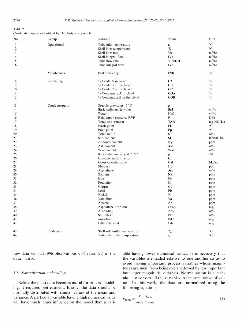
Table 2Candidate variables identified by Delphi-type approach

No. Group Variable Name Unit

1 Operational Tube inlet temperature ti �C2 Shell inlet temperature Ti �C3 Shell flow rate Vs m3/hr4 Shell integral flow IVc m3/hr5 Tube flow rate VPROD m3/hr6 Tube integral flow IVt m3/hr

7 Maintenance Peak efficiency IND %

8 Scheduling % Crude A in blend CA %9 % Crude B in the blend CB %

10 % Crude C in the blend CC %11 % Condensate A in blend COA %12 % Condensate B in the blend COB %

13 Crude property Specific gravity at 15 �C q –14 Basic sediment & water Sed vol%15 Water H2O vol%16 Reid vapor pressure, RVP P KPa17 Total acid number TAN mg KOH/g18 Flash point Fl �C19 Pour point Pp �C20 Total sulfur S wt%21 Salt content Sl lb/1000 bbl22 Nitrogen content N2 ppm23 Ash content Ash wt%24 Wax content Wax wt%25 Kinematic viscosity at 70 �C l cSt26 Characterization factor CF

27 Gross calorific value Cal MJ/kg28 Mercury Hg ppb29 Asphaltene Asp wt%30 Sodium Na ppm31 Iron Fe ppm32 Potassium K ppm33 Copper Cu ppm34 Lead Pb ppm35 Nickel Ni ppm36 Vanadium Va ppm37 Arsenic Ar ppm38 Asphaltene drop out Drop mg/l39 Aromatics Aro wt%40 Saturates PN wt%41 iso-octane ISO mg/l42 Filterable solid Fils mg/l

43 Predicates Shell side outlet temperature To �C44 Tube side outlet temperature to �C


raw data set had (996 observations · 44 variables) in thedata matrix.

3.3. Normalisation and scaling

Before the plant data becomes useful for process model-ing, it requires pretreatment. Ideally, the data should benormally distributed with similar values of the mean andvariance. A particular variable having high numerical valuewill have much larger influence on the model than a vari-

able having lower numerical values. It is necessary thatthe variables are scaled relative to one another so as toavoid having important process variables whose magni-tudes are small from being overshadowed by less importantbut larger magnitude variables. Normalisation is a tech-nique to convert all the variables to the same range of val-ues. In this work, the data are normalized using thefollowing equation:

xnorm ¼x� xmin

xmax � xmin

ð1Þ

Fig. 2. Score plot of first two principal components.


Being industrial data which are normally distributedwith mean at set points, variable transformation was notrequired.

3.4. Outlier removal and reduction of predictors

3.4.1. Principal component analysis (PCA)

Principal component analysis (PCA) identifies patternsin data, and expresses the data in such a way as to highlighttheir similarities and differences. Once these patterns havebeen found, the data can be compressed, i.e., number ofdimensions reduced, without much loss of information[29]. In the present work, PCA was used to remove outliersand to reduce the dimensionality of problem. Fig. 2 showsthe score plot of the first two principal components t[1] andt[2] generated using SIMCA-P software [29]. Similar plotsbetween t[1] with the subsequent principal componentst[3]. . .t[5] were also constructed. The ellipse in the diagramrepresents the Hotelling’s T2 at 95% confidence level. 63outliers lying outside the ellipse were identified andremoved, leaving 933 observations for the model develop-ment. Points lying close to each other in the score plot indi-cate the observations with similarities in their behaviour.For example, the cluster of points colored blue in Fig. 21

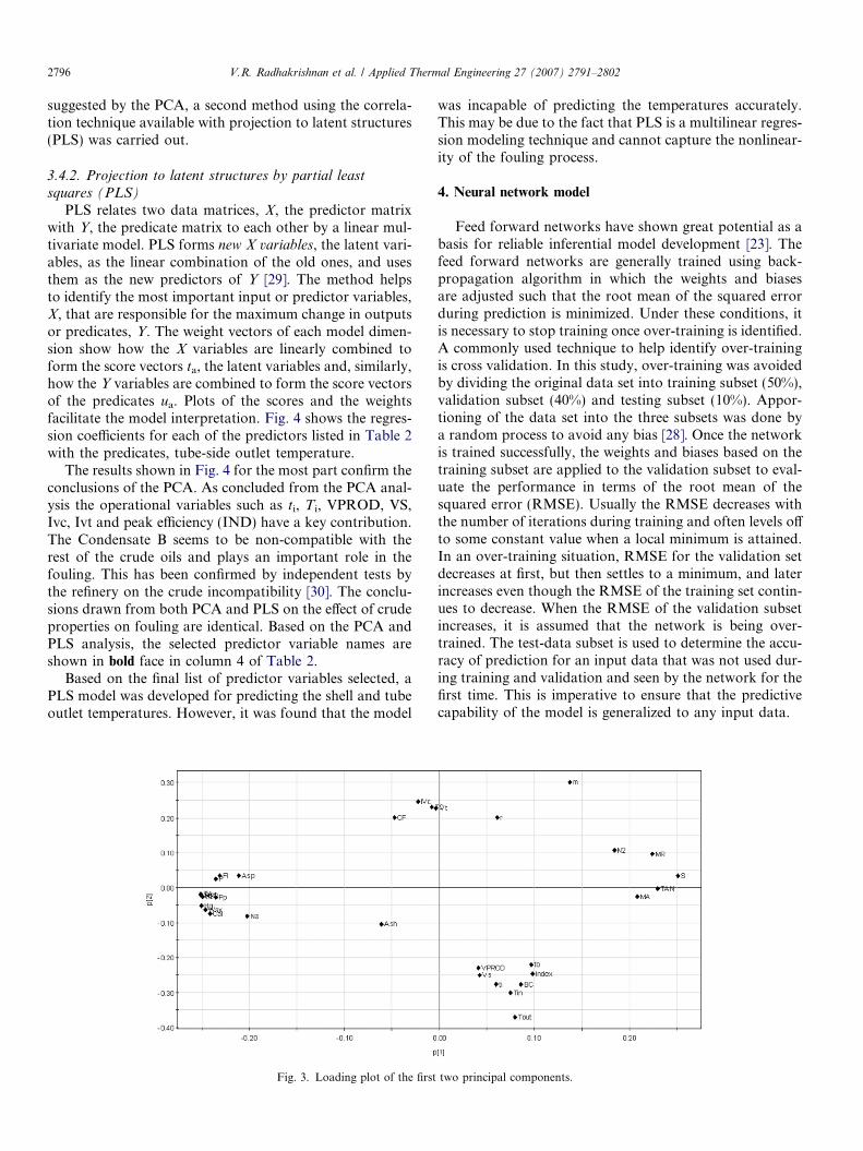
belongs to peak efficiency (IND) of one.A useful conclusion from the loading plot (Fig. 3) was

obtained by looking at the clustering of the variables. Itwas observed that a large number of crude properties arerelated with the percent of Crude A in the blend. Theseinclude basic sediments and water (Sed), salt (Sl), water

1 For interpretation of color in Fig. 2, the reader is referred to the webversion of the article.

(H2O), pour point (Pp), total acid number (TAN) and sul-fur (S). Similarly, mercury (Hg), wax content (Wax), andgross calorific value (Cal) lie close together. The third dis-tinct cluster consisted of flash point (Fl) and Reid vaporpressure (P). This is obviously because Crude A was themajor constituent of the blend used by the refinery and itplays a major role in the model. In view of the high corre-lation among some of these variables, the redundant vari-ables are omitted. Water (H2O) and salt (Sl) lie one overthe other and we may keep only one variable, say Sl. Sim-ilarly, between sulfur and total acid number, sulfur wasdropped. From among gross calorific value (Cal), mercury(Hg) and wax, wax was retained in the predictor set, drop-ping the other two variables. Flash point (Fl) was selectedfrom the third cluster. Minor mineral constituents such aspotassium, copper, lead, iron, nickel, vanadium and arsenicdid not play any significant role in the fouling process asevidenced by their non appearance in the loading plot. Sim-ilarly aromatics, saturates and iso-octane did not play anysignificant role. It was expected that filterable solids (Fils)and asphaltene drop out (Drop) to have a significant effect.However, there was insufficient data regarding these twovariables for the period of study and hence they couldnot be included in the model.

Another useful conclusion was that the blending ofother crudes such as COB, CB and CA contributed signif-icantly to the fouling as observed from the distance of thesepoints from the origin. The two integrated flow rates, Ivcand Ivt, are closely related as expected since both are timeintegral flows. The operational variables of shell- and tube-side flows and inlet and outlet temperatures formedanother cluster of variables. By the PCA analysis, the rela-tive importance of the different predictor variables on thepredicates is identified. Before dropping the variables


suggested by the PCA, a second method using the correla-tion technique available with projection to latent structures(PLS) was carried out.

3.4.2. Projection to latent structures by partial least

squares (PLS)

PLS relates two data matrices, X, the predictor matrixwith Y, the predicate matrix to each other by a linear mul-tivariate model. PLS forms new X variables, the latent vari-ables, as the linear combination of the old ones, and usesthem as the new predictors of Y [29]. The method helpsto identify the most important input or predictor variables,X, that are responsible for the maximum change in outputsor predicates, Y. The weight vectors of each model dimen-sion show how the X variables are linearly combined toform the score vectors ta, the latent variables and, similarly,how the Y variables are combined to form the score vectorsof the predicates ua. Plots of the scores and the weightsfacilitate the model interpretation. Fig. 4 shows the regres-sion coefficients for each of the predictors listed in Table 2with the predicates, tube-side outlet temperature.

The results shown in Fig. 4 for the most part confirm theconclusions of the PCA. As concluded from the PCA anal-ysis the operational variables such as ti, Ti, VPROD, VS,Ivc, Ivt and peak efficiency (IND) have a key contribution.The Condensate B seems to be non-compatible with therest of the crude oils and plays an important role in thefouling. This has been confirmed by independent tests bythe refinery on the crude incompatibility [30]. The conclu-sions drawn from both PCA and PLS on the effect of crudeproperties on fouling are identical. Based on the PCA andPLS analysis, the selected predictor variable names areshown in bold face in column 4 of Table 2.

Based on the final list of predictor variables selected, aPLS model was developed for predicting the shell and tubeoutlet temperatures. However, it was found that the model

Fig. 3. Loading plot of the first

was incapable of predicting the temperatures accurately.This may be due to the fact that PLS is a multilinear regres-sion modeling technique and cannot capture the nonlinear-ity of the fouling process.

4. Neural network model

Feed forward networks have shown great potential as abasis for reliable inferential model development [23]. Thefeed forward networks are generally trained using back-propagation algorithm in which the weights and biasesare adjusted such that the root mean of the squared errorduring prediction is minimized. Under these conditions, itis necessary to stop training once over-training is identified.A commonly used technique to help identify over-trainingis cross validation. In this study, over-training was avoidedby dividing the original data set into training subset (50%),validation subset (40%) and testing subset (10%). Appor-tioning of the data set into the three subsets was done bya random process to avoid any bias [28]. Once the networkis trained successfully, the weights and biases based on thetraining subset are applied to the validation subset to eval-uate the performance in terms of the root mean of thesquared error (RMSE). Usually the RMSE decreases withthe number of iterations during training and often levels offto some constant value when a local minimum is attained.In an over-training situation, RMSE for the validation setdecreases at first, but then settles to a minimum, and laterincreases even though the RMSE of the training set contin-ues to decrease. When the RMSE of the validation subsetincreases, it is assumed that the network is being over-trained. The test-data subset is used to determine the accu-racy of prediction for an input data that was not used dur-ing training and validation and seen by the network for thefirst time. This is imperative to ensure that the predictivecapability of the model is generalized to any input data.

two principal components.

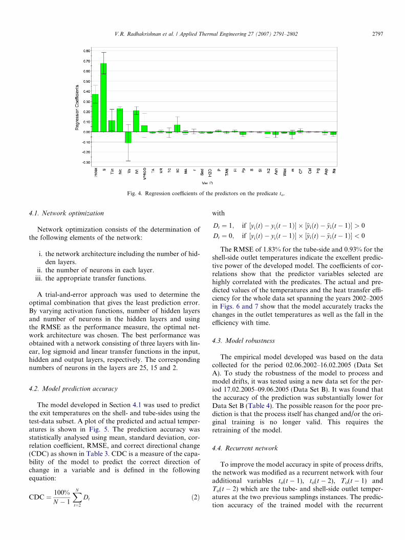
Fig. 4. Regression coefficients of the predictors on the predicate to.


4.1. Network optimization

Network optimization consists of the determination ofthe following elements of the network:

i. the network architecture including the number of hid-den layers.

ii. the number of neurons in each layer.iii. the appropriate transfer functions.

A trial-and-error approach was used to determine theoptimal combination that gives the least prediction error.By varying activation functions, number of hidden layersand number of neurons in the hidden layers and usingthe RMSE as the performance measure, the optimal net-work architecture was chosen. The best performance wasobtained with a network consisting of three layers with lin-ear, log sigmoid and linear transfer functions in the input,hidden and output layers, respectively. The correspondingnumbers of neurons in the layers are 25, 15 and 2.

4.2. Model prediction accuracy

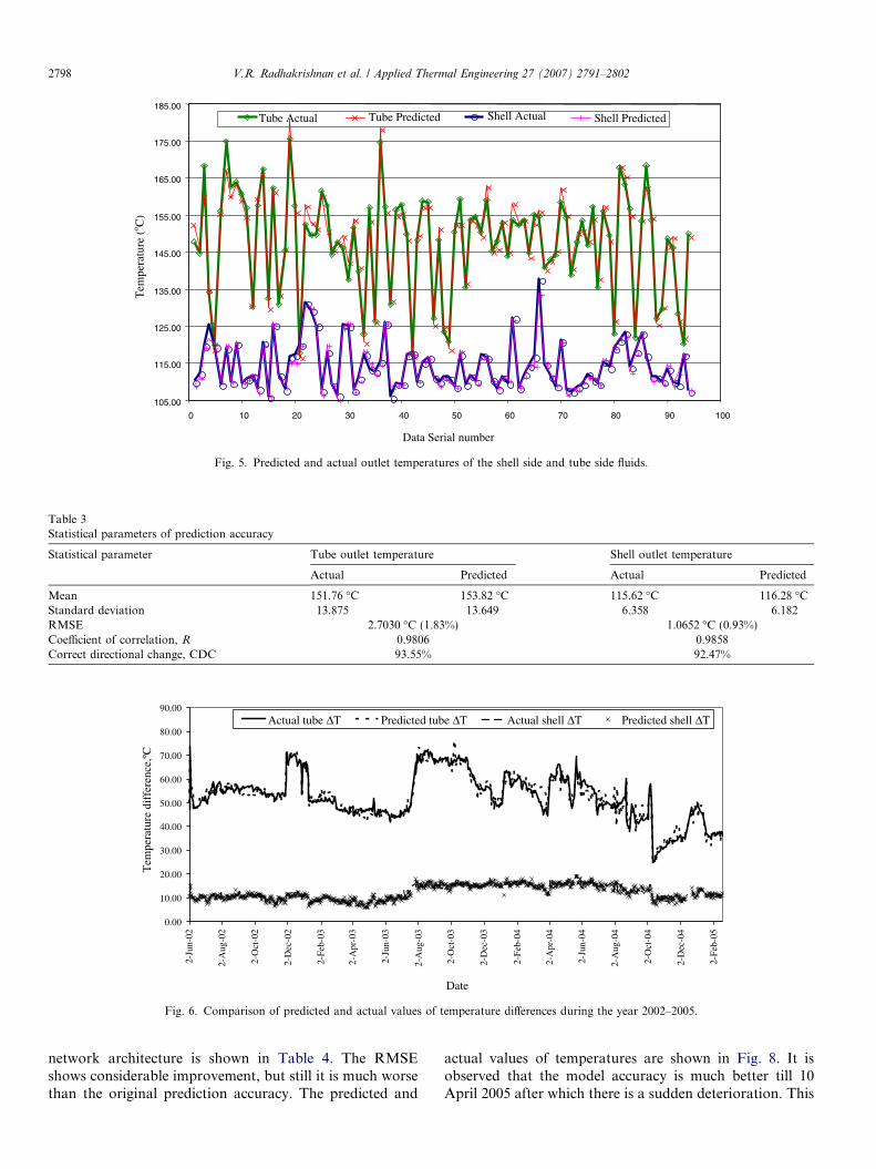
The model developed in Section 4.1 was used to predictthe exit temperatures on the shell- and tube-sides using thetest-data subset. A plot of the predicted and actual temper-atures is shown in Fig. 5. The prediction accuracy wasstatistically analysed using mean, standard deviation, cor-relation coefficient, RMSE, and correct directional change(CDC) as shown in Table 3. CDC is a measure of the capa-bility of the model to predict the correct direction ofchange in a variable and is defined in the followingequation:

CDC ¼ 100%

N � 1

XN

t¼2

Dt ð2Þ

with

Dt ¼ 1; if yiðtÞ � yiðt � 1Þ½ � � ~yiðtÞ � ~y iðt � 1Þ½ � > 0

Dt ¼ 0; if yiðtÞ � yiðt � 1Þ½ � � ~yiðtÞ � ~y iðt � 1Þ½ � < 0

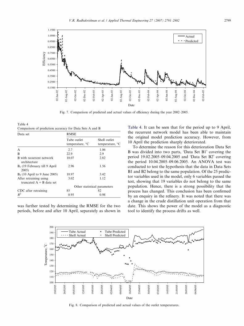
The RMSE of 1.83% for the tube-side and 0.93% for theshell-side outlet temperatures indicate the excellent predic-tive power of the developed model. The coefficients of cor-relations show that the predictor variables selected arehighly correlated with the predicates. The actual and pre-dicted values of the temperatures and the heat transfer effi-ciency for the whole data set spanning the years 2002–2005in Figs. 6 and 7 show that the model accurately tracks thechanges in the outlet temperatures as well as the fall in theefficiency with time.

4.3. Model robustness

The empirical model developed was based on the datacollected for the period 02.06.2002–16.02.2005 (Data SetA). To study the robustness of the model to process andmodel drifts, it was tested using a new data set for the per-iod 17.02.2005–09.06.2005 (Data Set B). It was found thatthe accuracy of the prediction was substantially lower forData Set B (Table 4). The possible reason for the poor pre-diction is that the process itself has changed and/or the ori-ginal training is no longer valid. This requires theretraining of the model.

4.4. Recurrent network

To improve the model accuracy in spite of process drifts,the network was modified as a recurrent network with fouradditional variables to(t � 1), to(t � 2), To(t � 1) andTo(t � 2) which are the tube- and shell-side outlet temper-atures at the two previous samplings instances. The predic-tion accuracy of the trained model with the recurrent

Data Serial number

105.00

115.00

125.00

135.00

145.00

155.00

165.00

175.00

185.00

0 10 20 30 40 50 60 70 80 90 100

Tube Actual Tube Predicted Shell Actual Shell Predicted

Tem

pera

ture

(o C

)

Fig. 5. Predicted and actual outlet temperatures of the shell side and tube side fluids.

Table 3Statistical parameters of prediction accuracy

Statistical parameter Tube outlet temperature Shell outlet temperature

Actual Predicted Actual Predicted

Mean 151.76 �C 153.82 �C 115.62 �C 116.28 �CStandard deviation 13.875 13.649 6.358 6.182RMSE 2.7030 �C (1.83%) 1.0652 �C (0.93%)Coefficient of correlation, R 0.9806 0.9858Correct directional change, CDC 93.55% 92.47%

0.00

10.00

20.00

30.00

40.00

50.00

60.00

70.00

80.00

90.00

2-Ju

n-02

2-A

ug-0

2

2-O

ct-0

2

2-D

ec-0

2

2-Fe

b-03

2-A

pr-0

3

2-Ju

n-03

2-A

ug-0

3

2-O

ct-0

3

2-D

ec-0

3

2-Fe

b-04

2-A

pr-0

4

2-Ju

n-04

2-A

ug-0

4

2-O

ct-0

4

2-D

ec-0

4

2-Fe

b-05

Date

Tem

pera

ture

dif

fere

nce,

ºC

Actual tube ΔT Predicted tube ΔT Actual shell ΔT Predicted shell ΔT

Fig. 6. Comparison of predicted and actual values of temperature differences during the year 2002–2005.


network architecture is shown in Table 4. The RMSEshows considerable improvement, but still it is much worsethan the original prediction accuracy. The predicted and

actual values of temperatures are shown in Fig. 8. It isobserved that the model accuracy is much better till 10April 2005 after which there is a sudden deterioration. This

0.1500

0.2500

0.3500

0.4500

0.5500

0.6500

0.7500

0.8500

0.9500

1.0500

1.1500

02-J

un-0

2

02-A

ug-0

2

02-O

ct-0

2

02-D

ec-0

2

02-F

eb-0

3

02-A

pr-0

3

02-J

un-0

3

02-A

ug-0

3

02-O

ct-0

3

02-D

ec-0

3

02-F

eb-0

4

02-A

pr-0

4

02-J

un-0

4

02-A

ug-0

4

02-O

ct-0

4

02-D

ec-0

4

02-F

eb-0

5

Date

Eff

icie

ncy

ActualPredicted

Fig. 7. Comparison of predicted and actual values of efficiency during the year 2002–2005.

Table 4Comparison of prediction accuracy for Data Sets A and B

Data set RMSE

Tube outlettemperature, �C

Shell outlettemperature, �C

A 2.7 1.06B 22.9 2.9B with recurrent network

architecture10.07 2.82

B1 (19 February till 9 April2005)

2.96 1.56

B2 (10 April to 9 June 2005) 10.97 3.42After retraining using

truncated A + B data set3.02 1.12

Other statistical parametersCDC after retraining 85 82R2 0.95 0.98


was further tested by determining the RMSE for the twoperiods, before and after 10 April, separately as shown in

100

110

120

130

140

150

160

170

180

190

200

19/0

2/05

26/0

2/05

05/0

3/05

12/0

3/05

19/0

3/05

26/0

3/05

02/0

4/05

09/0

4/05

D

Tem

pera

ture

,o C

Tube Actual Tube PredictedShell Actual Shell Predicted

Fig. 8. Comparison of predicted and actu

Table 4. It can be seen that for the period up to 9 April,the recurrent network model has been able to maintainthe original model prediction accuracy. However, from10 April the prediction sharply deteriorated.

To determine the reason for this deterioration Data SetB was divided into two parts, ‘Data Set B1’ covering theperiod 19.02.2005–09.04.2005 and ‘Data Set B2’ coveringthe period 10.04.2005–09.06.2005. An ANOVA test wasconducted to test the hypothesis that the data in Data SetsB1 and B2 belong to the same population. Of the 25 predic-tor variables used in the model, only 6 variables passed thetest, showing that 19 variables do not belong to the samepopulation. Hence, there is a strong possibility that theprocess has changed. This conclusion has been confirmedby an enquiry in the refinery. It was noted that there wasa change in the crude distillation unit operation from thatdate. This shows the power of the model as a diagnostictool to identify the process drifts as well.

16/0

4/05

23/0

4/05

30/0

4/05

07/0

5/05

14/0

5/05

21/0

5/05

28/0

5/05

04/0

6/05

ate

al values of the outlet temperatures.


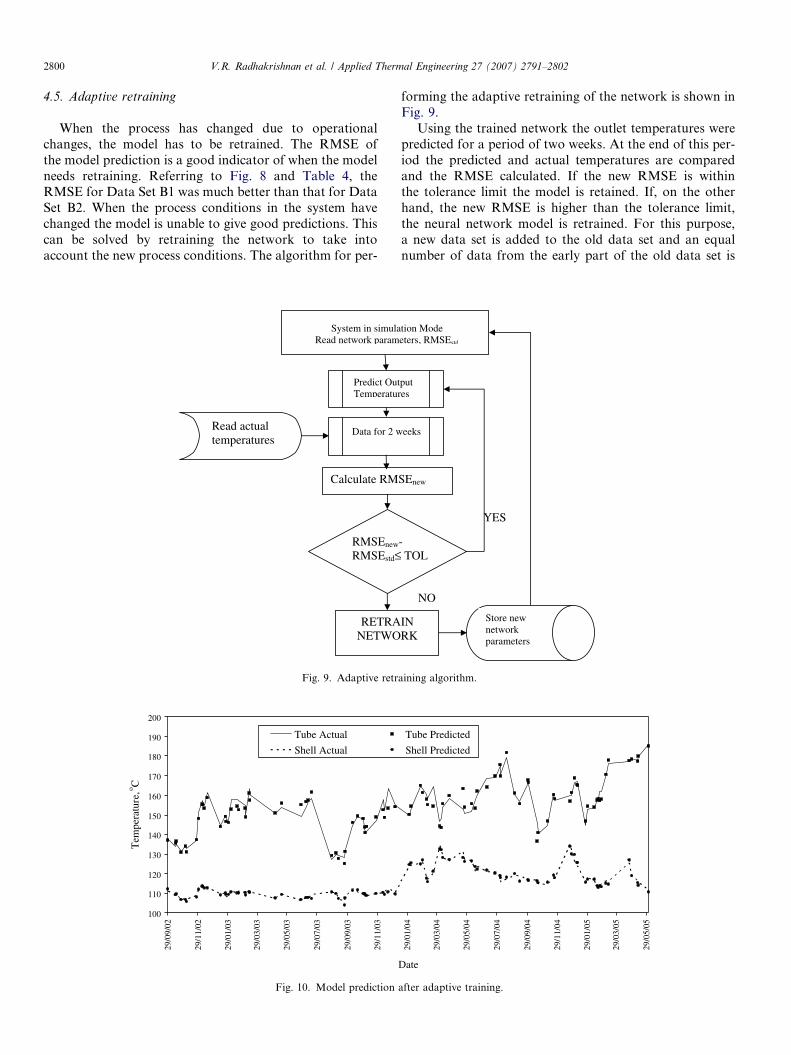
4.5. Adaptive retraining

When the process has changed due to operationalchanges, the model has to be retrained. The RMSE ofthe model prediction is a good indicator of when the modelneeds retraining. Referring to Fig. 8 and Table 4, theRMSE for Data Set B1 was much better than that for DataSet B2. When the process conditions in the system havechanged the model is unable to give good predictions. Thiscan be solved by retraining the network to take intoaccount the new process conditions. The algorithm for per-

Predict OutTemperatur

Read actual temperatures

Data for 2 w

RMSEnew

RMSEstd≤

Calculate RM

System in simulaRead network param

RETRANETWO

Fig. 9. Adaptive retr

100

110

120

130

140

150

160

170

180

190

200

29/0

9/02

29/1

1/02

29/0

1/03

29/0

3/03

29/0

5/03

29/0

7/03

29/0

9/03

29/1

1/03

Tem

pera

ture

,o C

Tube Actual

Shell Actual

Fig. 10. Model prediction

forming the adaptive retraining of the network is shown inFig. 9.

Using the trained network the outlet temperatures werepredicted for a period of two weeks. At the end of this per-iod the predicted and actual temperatures are comparedand the RMSE calculated. If the new RMSE is withinthe tolerance limit the model is retained. If, on the otherhand, the new RMSE is higher than the tolerance limit,the neural network model is retrained. For this purpose,a new data set is added to the old data set and an equalnumber of data from the early part of the old data set is

put es

eeks

- TOL

YES

SEnew

tion Mode eters, RMSEstd

NO

INRK

Store new networkparameters

aining algorithm.

29/0

1/04

29/0

3/04

29/0

5/04

29/0

7/04

29/0

9/04

29/1

1/04

29/0

1/05

29/0

3/05

29/0

5/05

Date

Tube Predicted

Shell Predicted

after adaptive training.


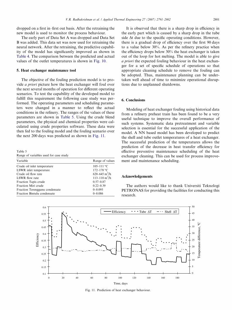
dropped on a first in–first out basis. After the retraining thenew model is used to monitor the process behaviour.

The early part of Data Set A was dropped and Data SetB was added. This data set was now used for retraining theneural network. After the retraining, the predictive capabil-ity of the model has significantly improved as shown inTable 4. The comparison between the predicted and actualvalues of the outlet temperatures is shown in Fig. 10.

5. Heat exchanger maintenance tool

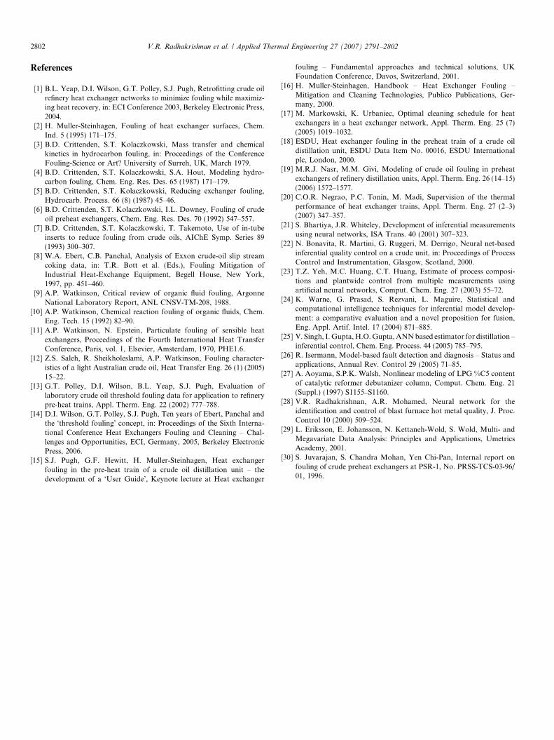
The objective of the fouling prediction model is to pro-vide a priori picture how the heat exchanger will foul overthe next several months of operation for different operatingscenarios. To test the capability of the developed model tofulfill this requirement the following case study was per-formed. The operating parameters and scheduling parame-ters were changed in a manner to reflect the actualconditions in the refinery. The ranges of the values of theseparameters are shown in Table 5. Using the crude blendparameters, the physical and chemical properties were cal-culated using crude properties software. These data werethen fed to the fouling model and the fouling scenario overthe next 200 days was predicted as shown in Fig. 11.

Table 5Range of variables used for case study

Variable Range of values

Crude oil inlet temperature 105–111 �CLSWR inlet temperature 172–178 �CCrude oil flow rate 620–645 m3/hLSWR flow rate 113–118 m3/hFraction Tapis crude 0.57–0.87Fraction Miri crude 0.22–0.39Fraction Terengganu condensate 0–0.095Fraction Bintulu condensate 0–0.086

0.1

0.15

0.2

0.25

0.3

0.35

0.4

0.45

0.5

0.55

0.6

0 20 40 60 80 10

Time,

Eff

icie

ncy

Efficie

Fig. 11. Prediction of heat

It is observed that there is a sharp drop in efficiency inthe early part which is caused by a sharp drop in the tubeside Dt due to the specific operating conditions. However,there is a gradual drop of efficiency over the first 90 daysto a value below 30%. As per the refinery practice whenthe efficiency drops below 30% the heat exchanger is takenout of the loop for hot melting. The model is able to givea priori the expected fouling behaviour in the heat exchan-ger for a set of specific schedule of operations so thatappropriate cleaning schedule to remove the fouling canbe adopted. Thus, maintenance planning can be under-taken well ahead of time to minimize operational disrup-tions due to unplanned shutdowns.

6. Conclusions

Modeling of heat exchanger fouling using historical datafrom a refinery preheat train has been found to be a veryuseful technique to improve the overall performance ofsuch systems. Systematic data pretreatment and variableselection is essential for the successful application of themodel. A NN based model has been developed to predictthe shell and tube outlet temperatures of a heat exchanger.The successful prediction of the temperatures allows theprediction of the decrease in heat transfer efficiency foreffective preventive maintenance scheduling of the heatexchanger cleaning. This can be used for process improve-ment and maintenance scheduling.

Acknowledgements

The authors would like to thank Universiti TeknologiPETRONAS for providing the facilities for conducting thisresearch.

0 120 140 160 180

days

0

5

10

15

20

25

30

35

40

45

50

Tem

pera

ture

dif

fere

nce,

ºC

ncy Tube ΔT Shell ΔT

exchanger behaviour.


References

[1] B.L. Yeap, D.I. Wilson, G.T. Polley, S.J. Pugh, Retrofitting crude oilrefinery heat exchanger networks to minimize fouling while maximiz-ing heat recovery, in: ECI Conference 2003, Berkeley Electronic Press,2004.

[2] H. Muller-Steinhagen, Fouling of heat exchanger surfaces, Chem.Ind. 5 (1995) 171–175.

[3] B.D. Crittenden, S.T. Kolaczkowski, Mass transfer and chemicalkinetics in hydrocarbon fouling, in: Proceedings of the ConferenceFouling-Science or Art? University of Surreh, UK, March 1979.

[4] B.D. Crittenden, S.T. Kolaczkowski, S.A. Hout, Modeling hydro-carbon fouling, Chem. Eng. Res. Des. 65 (1987) 171–179.

[5] B.D. Crittenden, S.T. Kolaczkowski, Reducing exchanger fouling,Hydrocarb. Process. 66 (8) (1987) 45–46.

[6] B.D. Crittenden, S.T. Kolaczkowski, I.L. Downey, Fouling of crudeoil preheat exchangers, Chem. Eng. Res. Des. 70 (1992) 547–557.

[7] B.D. Crittenden, S.T. Kolaczkowski, T. Takemoto, Use of in-tubeinserts to reduce fouling from crude oils, AIChE Symp. Series 89(1993) 300–307.

[8] W.A. Ebert, C.B. Panchal, Analysis of Exxon crude-oil slip streamcoking data, in: T.R. Bott et al. (Eds.), Fouling Mitigation ofIndustrial Heat-Exchange Equipment, Begell House, New York,1997, pp. 451–460.

[9] A.P. Watkinson, Critical review of organic fluid fouling, ArgonneNational Laboratory Report, ANL CNSV-TM-208, 1988.

[10] A.P. Watkinson, Chemical reaction fouling of organic fluids, Chem.Eng. Tech. 15 (1992) 82–90.

[11] A.P. Watkinson, N. Epstein, Particulate fouling of sensible heatexchangers, Proceedings of the Fourth International Heat TransferConference, Paris, vol. 1, Elsevier, Amsterdam, 1970, PHE1.6.

[12] Z.S. Saleh, R. Sheikholeslami, A.P. Watkinson, Fouling character-istics of a light Australian crude oil, Heat Transfer Eng. 26 (1) (2005)15–22.

[13] G.T. Polley, D.I. Wilson, B.L. Yeap, S.J. Pugh, Evaluation oflaboratory crude oil threshold fouling data for application to refinerypre-heat trains, Appl. Therm. Eng. 22 (2002) 777–788.

[14] D.I. Wilson, G.T. Polley, S.J. Pugh, Ten years of Ebert, Panchal andthe ‘threshold fouling’ concept, in: Proceedings of the Sixth Interna-tional Conference Heat Exchangers Fouling and Cleaning – Chal-lenges and Opportunities, ECI, Germany, 2005, Berkeley ElectronicPress, 2006.

[15] S.J. Pugh, G.F. Hewitt, H. Muller-Steinhagen, Heat exchangerfouling in the pre-heat train of a crude oil distillation unit – thedevelopment of a ‘User Guide’, Keynote lecture at Heat exchanger

fouling – Fundamental approaches and technical solutions, UKFoundation Conference, Davos, Switzerland, 2001.

[16] H. Muller-Steinhagen, Handbook – Heat Exchanger Fouling –Mitigation and Cleaning Technologies, Publico Publications, Ger-many, 2000.

[17] M. Markowski, K. Urbaniec, Optimal cleaning schedule for heatexchangers in a heat exchanger network, Appl. Therm. Eng. 25 (7)(2005) 1019–1032.

[18] ESDU, Heat exchanger fouling in the preheat train of a crude oildistillation unit, ESDU Data Item No. 00016, ESDU Internationalplc, London, 2000.

[19] M.R.J. Nasr, M.M. Givi, Modeling of crude oil fouling in preheatexchangers of refinery distillation units, Appl. Therm. Eng. 26 (14–15)(2006) 1572–1577.

[20] C.O.R. Negrao, P.C. Tonin, M. Madi, Supervision of the thermalperformance of heat exchanger trains, Appl. Therm. Eng. 27 (2–3)(2007) 347–357.

[21] S. Bhartiya, J.R. Whiteley, Development of inferential measurementsusing neural networks, ISA Trans. 40 (2001) 307–323.

[22] N. Bonavita, R. Martini, G. Ruggeri, M. Derrigo, Neural net-basedinferential quality control on a crude unit, in: Proceedings of ProcessControl and Instrumentation, Glasgow, Scotland, 2000.

[23] T.Z. Yeh, M.C. Huang, C.T. Huang, Estimate of process composi-tions and plantwide control from multiple measurements usingartificial neural networks, Comput. Chem. Eng. 27 (2003) 55–72.

[24] K. Warne, G. Prasad, S. Rezvani, L. Maguire, Statistical andcomputational intelligence techniques for inferential model develop-ment: a comparative evaluation and a novel proposition for fusion,Eng. Appl. Artif. Intel. 17 (2004) 871–885.

[25] V. Singh, I. Gupta, H.O. Gupta, ANN based estimator for distillation –inferential control, Chem. Eng. Process. 44 (2005) 785–795.

[26] R. Isermann, Model-based fault detection and diagnosis – Status andapplications, Annual Rev. Control 29 (2005) 71–85.

[27] A. Aoyama, S.P.K. Walsh, Nonlinear modeling of LPG %C5 contentof catalytic reformer debutanizer column, Comput. Chem. Eng. 21(Suppl.) (1997) S1155–S1160.

[28] V.R. Radhakrishnan, A.R. Mohamed, Neural network for theidentification and control of blast furnace hot metal quality, J. Proc.Control 10 (2000) 509–524.

[29] L. Eriksson, E. Johansson, N. Kettaneh-Wold, S. Wold, Multi- andMegavariate Data Analysis: Principles and Applications, UmetricsAcademy, 2001.

[30] S. Juvarajan, S. Chandra Mohan, Yen Chi-Pan, Internal report onfouling of crude preheat exchangers at PSR-1, No. PRSS-TCS-03-96/01, 1996.

Heat exchanger fouling model and preventive maintenance scheduling tool

Documents

Transcript of Heat exchanger fouling model and preventive maintenance scheduling tool