This article was downloaded by:[Technical University of Eindhoven][Technical University of Eindhoven]

On: 9 March 2007Access Details: [subscription number 731872791]Publisher: Taylor & FrancisInforma Ltd Registered in England and Wales Registered Number: 1072954Registered office: Mortimer House, 37-41 Mortimer Street, London W1T 3JH, UK

Heat Transfer EngineeringPublication details, including instructions for authors and subscription information:http://www.informaworld.com/smpp/title~content=t713723051

Validated Numerical Analysis of CaSO4 FoulingM. G. Mwaba a; C. C. M. Rindt a; A. A. Van Steenhoven a; M. A. G. Vorstman ba Department of Mechanical Engineering, Eindhoven University of Technology.Eindhoven. The Netherlandsb Department of Chemical Engineering, Eindhoven University of Technology.Eindhoven. The Netherlands

To link to this article: DOI: 10.1080/01457630600745160URL: http://dx.doi.org/10.1080/01457630600745160

Full terms and conditions of use: http://www.informaworld.com/terms-and-conditions-of-access.pdfThis article maybe used for research, teaching and private study purposes. Any substantial or systematic reproduction,re-distribution, re-selling, loan or sub-licensing, systematic supply or distribution in any form to anyone is expresslyforbidden.The publisher does not give any warranty express or implied or make any representation that the contents will becomplete or accurate or up to date. The accuracy of any instructions, formulae and drug doses should beindependently verified with primary sources. The publisher shall not be liable for any loss, actions, claims, proceedings,demand or costs or damages whatsoever or howsoever caused arising directly or indirectly in connection with orarising out of the use of this material.© Taylor and Francis 2007

Dow

nloa

ded

By: [

Tech

nica

l Uni

vers

ity o

f Ein

dhov

en] A

t: 16

:58

9 M

arch

200

7

Heat Transfer Engineering, 27(7):50–62, 2006Copyright C©© Taylor and Francis Group, LLCISSN: 0145-7632 print / 1521-0537 onlineDOI: 10.1080/01457630600745160

Validated Numerical Analysisof CaSO4 Fouling

M. G. MWABA, C. C. M. RINDT, and A. A. VAN STEENHOVENEindhoven University of Technology, Department of Mechanical Engineering, Eindhoven, The Netherlands

M. A. G. VORSTMANEindhoven University of Technology, Department of Chemical Engineering, Eindhoven, The Netherlands

In scaling experiments, the formation of fouling layers on heat transfer surfaces usually proceeds in a non-uniform manner.The result is a non-uniform layer, and hence a varying thermal resistance over the area covered with scale. Consequently, anon-uniform heat flux distribution results over the heat transfer surface. To evaluate the changes in the heat flow distributionresulting from a non-uniform scale layer, numerical calculations have been performed using a case where CaSO4 scalesform on a heated copper plate subjected to a shear flow. The calculated heat flux is used to calculate fouling resistances frommeasured temperatures. The results of the numerical calculations confirm that a non-uniform heat flux distribution occursover the surface when the plate is partially covered with scale. Further, it is seen that the heat flux, the surface temperature,and the driving force all decrease with increase in scale accumulation.

INTRODUCTION

Scaling, or crystallization fouling, is the accumulation ofsolid matter on a heat transfer surface due to crystallization. Inheat transfer equipment, scaling is normally encountered whenthe solubility limit of dissolved salts is exceeded under processconditions. Normal solubility salts cause scaling on cooled sur-faces, while inverse solubility salts lead to scaling on heatedsurfaces. Because the material of the scale layer is usually oflow thermal conductivity, its presence on a heat transfer sur-face leads to a reduction in the effectiveness of the heat transferequipment. Further, flow and thermal conditions prevailing inthe system coupled with the probabilistic nature of scale ini-tiation may lead to a scale layer developing in a non-uniformmanner.

A lack of models to accurately predict the rate at which de-posits form on heat transfer surfaces makes scaling a nuisanceto both designers and operators of heat exchange equipment.Designers need models that can help them to calculate the size

The authors acknowledge the Netherlands Organization for InternationalCooperation in Higher Education (Nuffic) for funding this project.

Address correspondence to Dr. M. G. Mwaba, Department of Mechanicaland Aerospace Engineering, Carleton University, 1125 Colonel By Dr., Ottawa,Ontario, K1S 5B6, Canada. E-mail: mmwaba@mae.carleton.ca

of heat transfer surfaces, and operators can utilize the models toaccurately predict the mean time between cleaning (MTBC). Inthe meantime, designers have to rely on values like those pub-lished in the TEMA standards [1] to accommodate scaling atthe design stage, while operators turn to experience as a guide indeciding when to shut down for cleaning. There is no doubt asto the potential benefits of deriving good predictive models. Todevelop such models, knowledge of the fundamental processesand parameters that affect scaling is required. Understandingthe underlying physics of the scaling process is a subject thatis currently receiving a lot of attention from researchers [2, 3].Most of the work is focused on experimental work. In experi-ments, however, not all required parameters can be measured.Parameters such as surface heat flux and surface temperatureare difficult to measure. Yet these parameters are paramountto unraveling the complexity of scaling. The influence of theseparameters on scaling can be analyzed by performing numeri-cal simulations. The objectives of this study were two-fold: tocomplement the experimental effort by numerically calculatingvariables that are difficult to measure, and to provide a simulationtool that can assist heat exchanger designers in evaluating the in-fluence of geometrical and physical parameters on heat transferrate.

In this paper, the simulation of scaling using simple mod-els is reported. The numerical results are used to accurately

50

Dow

nloa

ded

By: [

Tech

nica

l Uni

vers

ity o

f Ein

dhov

en] A

t: 16

:58

9 M

arch

200

7

M. G. MWABA ET AL. 51

calculate fouling resistance to heat transfer as a function of timeand position.

PROBLEM STATEMENT

In scaling experiments, a commonly used approach is to mea-sure changes in the thermal system and estimate the thermalresistance arising from the presence of a scale layer. Such anapproach is realized by using a pair of thermocouples: one ther-mocouple suspended in the bulk and the second placed in thewall, very near to the surface. For such an arrangement the re-sistance of the scale, R f,x , at each position is determined from:

R f,x =(

Tw,x − Tb

q ′′

)t

−(

Tw,x − Tb

q ′′

)0

(1)

where Tw,x and Tb are the wall and bulk temperatures respec-tively, and q ′′ is the heat flux. The subscripts t and 0 representthe conditions at present time and initial time, respectively.

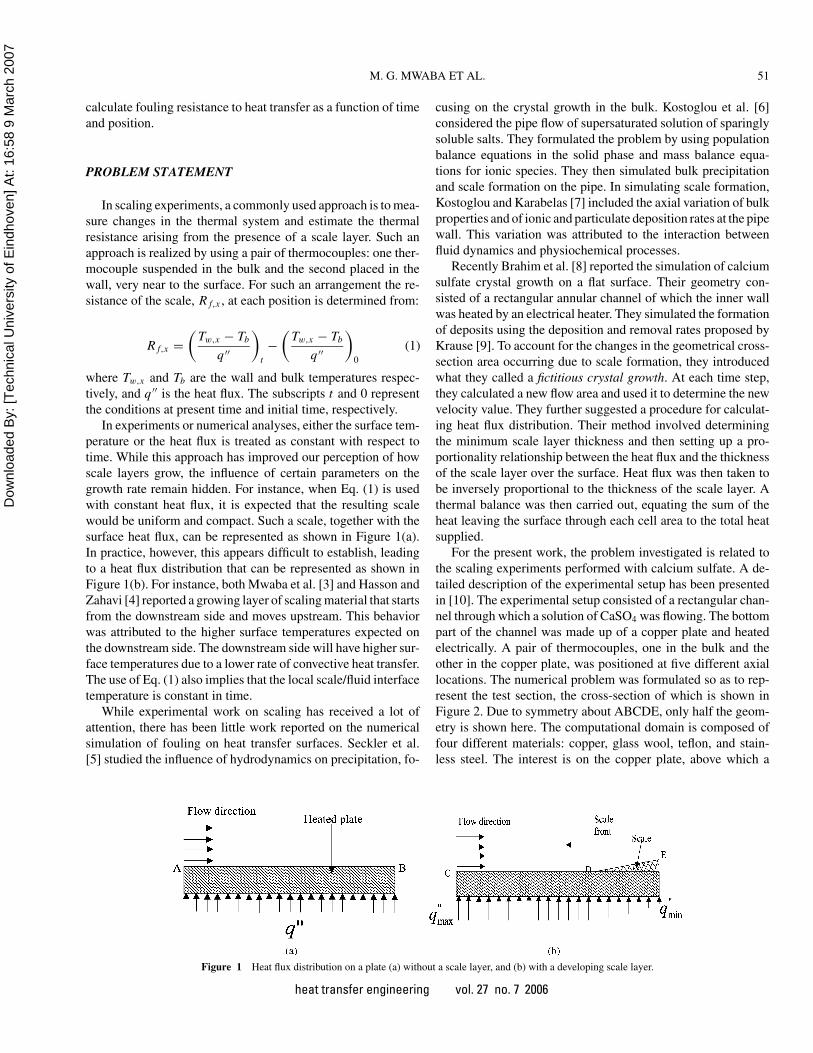
In experiments or numerical analyses, either the surface tem-perature or the heat flux is treated as constant with respect totime. While this approach has improved our perception of howscale layers grow, the influence of certain parameters on thegrowth rate remain hidden. For instance, when Eq. (1) is usedwith constant heat flux, it is expected that the resulting scalewould be uniform and compact. Such a scale, together with thesurface heat flux, can be represented as shown in Figure 1(a).In practice, however, this appears difficult to establish, leadingto a heat flux distribution that can be represented as shown inFigure 1(b). For instance, both Mwaba et al. [3] and Hasson andZahavi [4] reported a growing layer of scaling material that startsfrom the downstream side and moves upstream. This behaviorwas attributed to the higher surface temperatures expected onthe downstream side. The downstream side will have higher sur-face temperatures due to a lower rate of convective heat transfer.The use of Eq. (1) also implies that the local scale/fluid interfacetemperature is constant in time.

While experimental work on scaling has received a lot ofattention, there has been little work reported on the numericalsimulation of fouling on heat transfer surfaces. Seckler et al.[5] studied the influence of hydrodynamics on precipitation, fo-

Figure 1 Heat flux distribution on a plate (a) without a scale layer, and (b) with a developing scale layer.

cusing on the crystal growth in the bulk. Kostoglou et al. [6]considered the pipe flow of supersaturated solution of sparinglysoluble salts. They formulated the problem by using populationbalance equations in the solid phase and mass balance equa-tions for ionic species. They then simulated bulk precipitationand scale formation on the pipe. In simulating scale formation,Kostoglou and Karabelas [7] included the axial variation of bulkproperties and of ionic and particulate deposition rates at the pipewall. This variation was attributed to the interaction betweenfluid dynamics and physiochemical processes.

Recently Brahim et al. [8] reported the simulation of calciumsulfate crystal growth on a flat surface. Their geometry con-sisted of a rectangular annular channel of which the inner wallwas heated by an electrical heater. They simulated the formationof deposits using the deposition and removal rates proposed byKrause [9]. To account for the changes in the geometrical cross-section area occurring due to scale formation, they introducedwhat they called a fictitious crystal growth. At each time step,they calculated a new flow area and used it to determine the newvelocity value. They further suggested a procedure for calculat-ing heat flux distribution. Their method involved determiningthe minimum scale layer thickness and then setting up a pro-portionality relationship between the heat flux and the thicknessof the scale layer over the surface. Heat flux was then taken tobe inversely proportional to the thickness of the scale layer. Athermal balance was then carried out, equating the sum of theheat leaving the surface through each cell area to the total heatsupplied.

For the present work, the problem investigated is related tothe scaling experiments performed with calcium sulfate. A de-tailed description of the experimental setup has been presentedin [10]. The experimental setup consisted of a rectangular chan-nel through which a solution of CaSO4 was flowing. The bottompart of the channel was made up of a copper plate and heatedelectrically. A pair of thermocouples, one in the bulk and theother in the copper plate, was positioned at five different axiallocations. The numerical problem was formulated so as to rep-resent the test section, the cross-section of which is shown inFigure 2. Due to symmetry about ABCDE, only half the geom-etry is shown here. The computational domain is composed offour different materials: copper, glass wool, teflon, and stain-less steel. The interest is on the copper plate, above which a

heat transfer engineering vol. 27 no. 7 2006

Dow

nloa

ded

By: [

Tech

nica

l Uni

vers

ity o

f Ein

dhov

en] A

t: 16

:58

9 M

arch

200

7

52 M. G. MWABA ET AL.

Figure 2 Arrangement of thermocouples (left) and cross-section of the problem domain (right). Dimensions are in millimetres.

supersaturated solution of calcium sulfate was flowing. The platehad a width of 14 mm and a length of 600 mm. The plate washeated by an electrical heater of which the center axis was posi-tioned at a distance of 25 mm below the surface. The electricalheater, with unheated lengths on either side, was in contact withthe copper plate on curve BC and supplied with constant electri-cal power. The unheated lengths were 60 mm on the flow inletside and 5 mm on the exit side. The copper plate was insulatedusing glass wool with a thickness of approximately 5 mm. Fur-ther, the copper plate was separated from the stainless steelhousing by a teflon strip, 5 mm in thickness. The initial bulkconcentration, the inlet velocity, and the bulk temperature wereknown. The task at hand was to predict the rate of deposit for-mation and calculate the heat flux and the surface temperatureat the solid-liquid interface.

The problem was formulated subject to the following assump-tions:

• The surface of the plate was assumed to be smooth. This as-sumption enabled the use of published heat transfer coefficientcorrelations for smooth surfaces.

• The heat transfer coefficient was assumed to vary only in theflow direction.

• The surface of the scale layer was smooth and its presencedid not change the flow conditions.

• Scale movement was assumed to be governed by nuclea-tion for lateral movement and crystal growth for layerthickness.

• The probabilistic nature of nucleation was neglected. Nucle-ation was assumed to commence at the exit side of the plateand then move upstream. A simple model derived from ex-perimental measurements was used to track the movement ofthe nucleation front.

• The scale was assumed to adhere very strongly to the plate,rendering its removal less important. This assumption is basedon experimental evidence showing that removal was restrictedto a thin layer lying on top of a strong adherent layer [3].

• Because scaling is a very slow process, temperature changesin the solids were assumed to be quasi steady.

• Crystals forming on the surface were of the gypsum phase.

A three-dimensional conduction problem was formulated andsolved using the commercial software package CFX. The growthof the scale layer was modeled as a time-dependent resistanceon top of the copper surface. The fluid-to-wall heat transfercoefficient varied axially due to thermal entrance effects.

MODELS FOR NUCLEATION AND GROWTH RATES

The source of the crystals forming on a heated plate are theions, originally dissolved in the flowing fluid. Crystal formationtakes place only when the dissolved species are in a supersat-urated state and is governed by two kinetic processes, nucle-ation and crystal growth. Nucleation refers to the formation ofminute particles. Various types of nucleation have been identi-fied and a comprehensive review can be found elsewhere [11].When nuclei form on a foreign body, it is referred to as hetero-geneous nucleation. It is this type of nucleation that occurs inheat exchange systems. In general, heterogeneous nucleation ona foreign substrate can be calculated from:

J = A′ exp

(− 16πN V 2

m σ3

3R 3g T 3

i (ln S)2

)(2)

where A′ is the pre-exponential factor, N is Avogadro’s number,Vm is the molar volume, σ is the specific interfacial energy, Rg

is the universal gas constant, Ti is the solid/liquid interface tem-perature, and S is the supersaturation. Supersaturation is definedas:

S = Cb

Cs(3)

where Cb and Cs are the bulk concentration and saturationconcentration, respectively. Saturation concentration is obtained

heat transfer engineering vol. 27 no. 7 2006

Dow

nloa

ded

By: [

Tech

nica

l Uni

vers

ity o

f Ein

dhov

en] A

t: 16

:58

9 M

arch

200

7

M. G. MWABA ET AL. 53

from the solubility curve for gypsum [12]. By using curve-fittingtechniques on the solubility curve for gypsum, an expression forthe saturation concentration is obtained as:

Cs (Ti ) = 2.0 × 10−6 (Ti − 273)3 − 4.0 × 10−4 (Ti − 273)2

+ 0.0222 (Ti − 273) + 1.7557 (4)

where Ti is the temperature at the solid-liquid interface expressedin K. Equation (4) is valid for the temperature range 313 K to363 K.

Scale formation has been observed to commence from thedownstream end moving toward the upstream end (seeFigure 1b). The lateral movement of the scale and the increase inlayer thickness are due to a combination of complex mechanismsthat may include nucleation, agglomeration, crystal growth, re-moval, and aging. A procedure used for monitoring the move-ment of the nucleation front is now explained.

The stochastic nature of nucleation and the lack of accurateknowledge of the many factors that influence initiation of nu-cleate formation make it difficult to predict the position wherenucleation will start. Data from experiments [10] in combina-tion with an empirical expression for induction time have beenused to formulate an expression for monitoring the nucleationfront. The experimental results showed that nucleation and sub-sequently growth of crystals started at different times on theplate. Fouling curves generated by plotting fouling resistanceagainst time at five measuring points were examined. The timetaken for each fouling curve to cross the abscissa was taken asthe local induction time. Induction time, tind, can be related tosupersaturation by the following expression [13]:

ln (tind) = ln (B1) + B2

(ln S)2 (5)

where B1 is an empirical constant and B2 depends on a numberof variables, and is given by:

B2 = aσ3V 2m N f (θ)(

2.3RgTi)3 (6)

where a is a geometrical factor and f(θ) is a correction factor,taken as unity for homogeneous nucleation and 0.01 for hetero-geneous nucleation.

The local supersaturation at each measuring point was cal-culated using Eqs. (3) and (4). Plots of ln(tind) against 1/(ln S)2

were used to obtain B1 and B2, giving the empirical expressionfor the induction time as:

tind = 7.36 exp

[0.1668

(ln S)2

](7)

The application of Eq. (7) to the results in [10] showed thatthe position of the nucleation front can be predicted by:

xfront = −3.0 × 10−4tind + 1.5 (8)

Equation (8) is valid for 0 < xfront < 0.6, and was used totrack the position of the nucleation front on the heated plate.

Nucleation front forms when xfront = 0 and ceases when xfront =0.6.

The process of nucleation is followed by crystal growth. Var-ious models have been proposed to describe crystal growth. Forinstance, in [14], it has been shown that the rate of mass depositedper unit area of heat transfer surface due to crystallization, in theabsence of removal, is:

dm ′

dt= β

[1

2

(β

kr

)+ (Cb − Cs)

−√

1

4

(β

kr

)2

+(

β

kr

)(Cb − Cs)

](9)

whereβ is the mass transfer coefficient and kr is the rate constant.The mass transfer coefficient can be obtained from the Sher-

wood relation:

Shx = 0.023 Re0.8Sc0.33

(1 + 6dh

x

)(10)

with the Sherwood number defined as Sh = βdh/Dl , whereDl is the diffusivity of the ions and dh is the hydraulic diameter.Entrance effects are accounted for by using the guidelines similarto those given for the heat transfer coefficient, as explained laterusing Eqs. (14) and (15).

The expression for the rate constant kr calculated from theexperimental results (as explained in [10]) is:

kr = 93900 exp

(−7820

Ti

)(11)

NUMERICAL MODELS

Temperature Model

Scaling is a very slow process, and changes in the thermalsystem arising from scale formation are correspondingly slow.On the basis of this, temperature changes in the solids can betreated as quasi-steady, allowing the problem to be treated assteady-state conduction. Steady-state conduction is governed bythe Laplace equation, which can be expressed as:

∂2T

∂x2+ ∂2T

∂y2+ ∂2T

∂z2= 0 (12)

The heat flux is given by Fourier’s law:

q ′′ = −λ∇T (13)

where λ is the material thermal conductivity and ∇T is thetemperature gradient. The temperature gradient can be obtainedfrom knowledge of the temperature distribution, which in turnis obtained by solving Eq. (12) subject to appropriate boundaryand initial conditions.

heat transfer engineering vol. 27 no. 7 2006

Dow

nloa

ded

By: [

Tech

nica

l Uni

vers

ity o

f Ein

dhov

en] A

t: 16

:58

9 M

arch

200

7

54 M. G. MWABA ET AL.

Table 1 Initial conditions

Parameter Value

Copper plate temperature, Tw 303 KInsulation wall temperature, Ts,air 323 KInlet fluid temperature, Tb 313 KAir temperature, Tb,air 293 KInlet bulk concentration, Cb 3.0 kg/m3

Heat flux, q ′′ q ′′ = 93 kW/m2

Nucleation front xfront = 0 m

Initial and Boundary Conditions

The initial conditions used are straightforward and are sum-marized in Table 1. Boundary conditions, presented in Table 2,on the other hand need to be explained. On surfaces AO, ON,NM, ML, LK, and KJ (see Figure 2), the test section was incontact with air, and the heat losses occurred by a combinationof natural convection and radiation. Heat loss due to each ofthe mechanisms was estimated. The total heat loss obtained wasused to estimate an equivalent heat transfer coefficient to use inthe Robin-type boundary condition on these surfaces. The valueobtained was Ueff = 7.0 W/m2 K.

The CaSO4 solution was in contact with the test section onsurfaces DF, FG, GH, and HI; hence, heat transfer was by con-vection. Here, the heat transfer coefficient was adjusted to ac-commodate entrance effects. The following guideline was pro-posed for use when calculating the heat transfer coefficient inshort ducts [15]:

Nux = 0.023 Re0.8Pr0.4

(1 +

(dh

x

)0.7)

(14)

for 2 < xdh

< 20, and

Nux = 0.023 Re0.8Pr0.4

(1 + 6dh

x

)(15)

for 20 < xdh

< 60.Equations (14) and (15) are valid for variable velocity and

temperature profiles along the axis of flow. For the problemunder consideration, the flow is fully developed while the ther-mal boundary layer is still developing. No model was found inliterature for a case with a fully developed velocity boundarylayer and a developing thermal boundary layer. Therefore, itwas decided to use the above expressions for this case. The testsection used had a length of 600 mm and a hydraulic diameterof 23.7 mm, giving the length-to-diameter ratio, L/dh , as 25.3.However, both equations cannot be used together over the en-

Table 2 Boundary conditions

Portion (with reference to Figure 2) Boundary condition

AB, CD, Front and Back Symmetry plane: ∇T = 0Curve BC Heat Flux, q ′′ = 93 kW/m2

DF, FG, GH, and HI q ′′ = U (Tw − Tb)AO, ON, NM, ML, LK, and KJ q ′′ = Ueff(Ts,air − Tb,air)

Figure 3 Measured and numerically calculated surface temperature in theabsence of a scale layer at Re = 23,000.

tire plate, as doing so introduces a discontinuity at x/dh = 20.The selection of the appropriate equation was made on the basisof the initial surface temperatures. Initial surface temperaturesare important because they influence both the rate of nucle-ation and the rate constant for crystallization. In [10], the build-up of a fouling layer was observed to start in the downstreamregion of the heated plate (20 < x/dh < 25.3). To simulatethe beginning of the scaling process, accurate temperatures aretherefore needed in this region. Figure 3 shows plots of themeasured temperatures and of the temperatures calculated withEqs. (14) and (15). It is seen that the temperatures calculatedwith Eq. (15) show a better agreement with the measured val-ues in the region where fouling begins. Equation (15) is there-fore selected and used over the entire plate. The implication ofthis choice is that the heat transfer coefficient is over-predicted,and the surface temperature is under-predicted for the regionx/dh < 20.

The local overall thermal resistance, 1/Ux , on the face wherethe CaSO4 solution was flowing is equal to the sum of the con-vection resistance and the fouling resistance:

1

Ux= 1

hx+ R f,x (16)

where Ux is the overall heat transfer coefficient at position x .To calculate R f,x , a scaling model was required. Details of thescaling model used are given in the next section.

Scaling Model

The rate of scaling is described by Eq. (9), which is a modi-fication of the scaling model that was first proposed by Bohnet[14]. A major modification was the omission of the removal

heat transfer engineering vol. 27 no. 7 2006

Dow

nloa

ded

By: [

Tech

nica

l Uni

vers

ity o

f Ein

dhov

en] A

t: 16

:58

9 M

arch

200

7

M. G. MWABA ET AL. 55

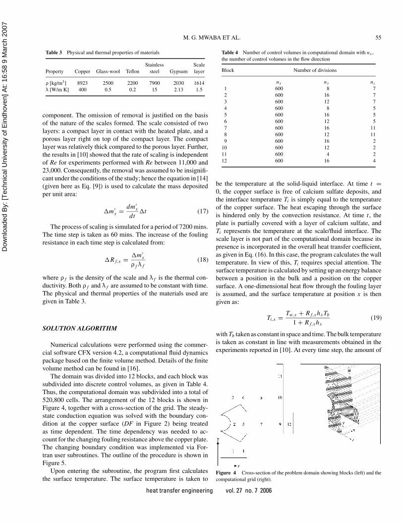
Table 3 Physical and thermal properties of materials

Stainless ScaleProperty Copper Glass-wool Teflon steel Gypsum layer

ρ [kg/m3] 8923 2500 2200 7900 2030 1614λ [W/m K] 400 0.5 0.2 15 2.13 1.5

component. The omission of removal is justified on the basisof the nature of the scales formed. The scale consisted of twolayers: a compact layer in contact with the heated plate, and aporous layer right on top of the compact layer. The compactlayer was relatively thick compared to the porous layer. Further,the results in [10] showed that the rate of scaling is independentof Re for experiments performed with Re between 11,000 and23,000. Consequently, the removal was assumed to be insignifi-cant under the conditions of the study; hence the equation in [14](given here as Eq. [9]) is used to calculate the mass depositedper unit area:

�m ′x = dm ′

x

dt�t (17)

The process of scaling is simulated for a period of 7200 mins.The time step is taken as 60 mins. The increase of the foulingresistance in each time step is calculated from:

�R f,x = �m ′x

ρ f λ f(18)

where ρ f is the density of the scale and λ f is the thermal con-ductivity. Both ρ f and λ f are assumed to be constant with time.The physical and thermal properties of the materials used aregiven in Table 3.

SOLUTION ALGORITHM

Numerical calculations were performed using the commer-cial software CFX version 4.2, a computational fluid dynamicspackage based on the finite volume method. Details of the finitevolume method can be found in [16].

The domain was divided into 12 blocks, and each block wassubdivided into discrete control volumes, as given in Table 4.Thus, the computational domain was subdivided into a total of520,800 cells. The arrangement of the 12 blocks is shown inFigure 4, together with a cross-section of the grid. The steady-state conduction equation was solved with the boundary con-dition at the copper surface (DF in Figure 2) being treatedas time dependent. The time dependency was needed to ac-count for the changing fouling resistance above the copper plate.The changing boundary condition was implemented via For-tran user subroutines. The outline of the procedure is shown inFigure 5.

Upon entering the subroutine, the program first calculatesthe surface temperature. The surface temperature is taken to

Table 4 Number of control volumes in computational domain with nx ,the number of control volumes in the flow direction

Block Number of divisions

nx ny nz

1 600 8 72 600 16 73 600 12 74 600 8 55 600 16 56 600 12 57 600 16 118 600 12 119 600 16 2

10 600 12 211 600 4 212 600 16 4

be the temperature at the solid-liquid interface. At time t =0, the copper surface is free of calcium sulfate deposits, andthe interface temperature Ti is simply equal to the temperatureof the copper surface. The heat escaping through the surfaceis hindered only by the convection resistance. At time t , theplate is partially covered with a layer of calcium sulfate, andTi represents the temperature at the scale/fluid interface. Thescale layer is not part of the computational domain because itspresence is incorporated in the overall heat transfer coefficient,as given in Eq. (16). In this case, the program calculates the walltemperature. In view of this, Ti requires special attention. Thesurface temperature is calculated by setting up an energy balancebetween a position in the bulk and a position on the coppersurface. A one-dimensional heat flow through the fouling layeris assumed, and the surface temperature at position x is thengiven as:

Ti,x = Tw,x + R f,x hx Tb

1 + R f,x hx(19)

with Tb taken as constant in space and time. The bulk temperatureis taken as constant in line with measurements obtained in theexperiments reported in [10]. At every time step, the amount of

Figure 4 Cross-section of the problem domain showing blocks (left) and thecomputational grid (right).

heat transfer engineering vol. 27 no. 7 2006

Dow

nloa

ded

By: [

Tech

nica

l Uni

vers

ity o

f Ein

dhov

en] A

t: 16

:58

9 M

arch

200

7

56 M. G. MWABA ET AL.

Figure 5 Flowchart of the calculation procedure.

mass deposited on each cell face is calculated using Eq. (17).Next, the resistance is calculated using Eq. (18). The new valueof R f,x is then substituted in Eq. (16) to calculate the overallheat transfer coefficient for the new time step.

The decrease in bulk concentration is proportional to theamount of mass deposited on the plate. The total mass depositedin unit time is determined by summing the mass deposited oneach nodal face. This is then subtracted from the mass of solutepresent in the bulk, and a new value of the bulk concentration isfound from

Cb(t + �t) = Cb(t) − 1

V

n∑i=1

�m ′i�xi�zi (20)

where V is the total volume of the calcium sulfate solutionpresent in the system, n is the number of cells on the surface,and the product of �x and �z is the area of a computational

cell. Because the axial variation of bulk concentration is verysmall, it is assumed to be constant over the plate length at eachtime step. The procedure is repeated until the specified time isattained.

RESULTS

The formation of deposits on a heat transfer surface may resultin changes to the heat flux and surface temperature distributions.The deposit formation was simulated by considering a CaSO4

solution flowing over a heated copper plate. The results obtainedare presented below.

Numerical Results

Heat Flux

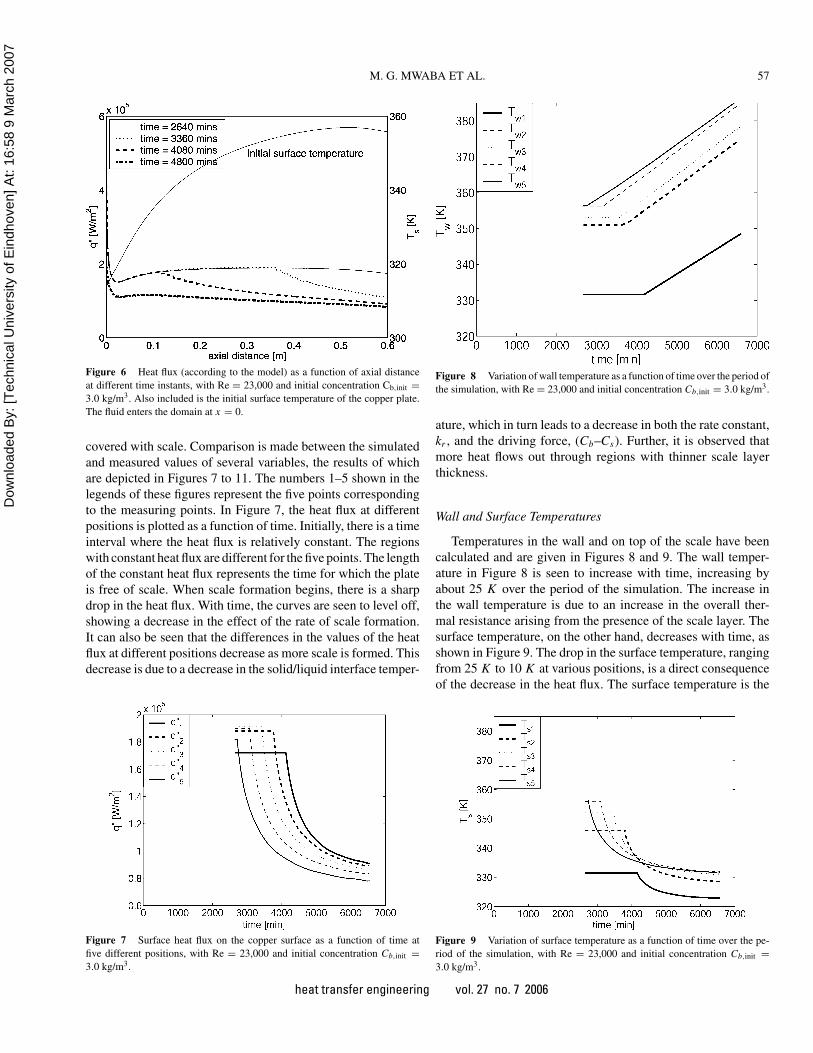
Surface heat flux has been calculated on the surface in con-tact with the fluid. In Figure 6, the surface heat flux in the axialdirection is shown for different time instants. Included in thisfigure is the surface temperature before the commencement ofdeposit formation. The thick solid line represents the heat fluxwhen the plate is free of scale. Three regions can be identi-fied. The first region is that of very high heat flux, occurringat the beginning of the plate. The high heat flux here is dueto the theoretically infinitely high heat transfer coefficient atx = 0 (see Eq. [15]). Because of the high heat transfer coeffi-cient in this region and the no-heat zone in the first 60 mm, thesurface temperature is low, approaching the bulk temperatureof the solution. In the region between 0.05 mm and 0.2 mm,the heat flux increases steadily and becomes constant, due tothe decreasing influence of the entrance effects and the attain-ment of a balance between heat input and heat convected awayby the fluid. For points 0.2 mm to 0.5 mm, the heat flux isrelatively constant. Toward the end of the plate, the heat fluxstarts decreasing, mainly due to the presence of the no-heatzone.

In Figure 6, the non-solid lines represent the heat flux dis-tribution when the plate has a scale layer on it. The dotted lineshows a decrease in the heat flux after 0.36 m. The part wherethe decrease is observed corresponds with the region on the platethat is covered by a scale layer. The heat flux reduction observedis due to the high resistance of the scale layer. A similar trend isobserved with the other curves. The heat flux reduces where thescale deposits have formed. The last curve represents conditionswhen the plate is fully covered with scale. Here the decrease ofheat flux in the axial direction is gradual. In general, the surfaceheat flux decreases with an increase in the scale layer thickness.With a constant heat flux boundary condition, the surface heatflux should remain constant. In this case, however, the surfaceheat flux decreases because more heat is lost to the environmentas scaling progresses. The results in Figure 6 further show thatthe flux distribution tends to be uniform when the entire plate is

heat transfer engineering vol. 27 no. 7 2006

Dow

nloa

ded

By: [

Tech

nica

l Uni

vers

ity o

f Ein

dhov

en] A

t: 16

:58

9 M

arch

200

7

M. G. MWABA ET AL. 57

Figure 6 Heat flux (according to the model) as a function of axial distanceat different time instants, with Re = 23,000 and initial concentration Cb,init =3.0 kg/m3. Also included is the initial surface temperature of the copper plate.The fluid enters the domain at x = 0.

covered with scale. Comparison is made between the simulatedand measured values of several variables, the results of whichare depicted in Figures 7 to 11. The numbers 1–5 shown in thelegends of these figures represent the five points correspondingto the measuring points. In Figure 7, the heat flux at differentpositions is plotted as a function of time. Initially, there is a timeinterval where the heat flux is relatively constant. The regionswith constant heat flux are different for the five points. The lengthof the constant heat flux represents the time for which the plateis free of scale. When scale formation begins, there is a sharpdrop in the heat flux. With time, the curves are seen to level off,showing a decrease in the effect of the rate of scale formation.It can also be seen that the differences in the values of the heatflux at different positions decrease as more scale is formed. Thisdecrease is due to a decrease in the solid/liquid interface temper-

Figure 7 Surface heat flux on the copper surface as a function of time atfive different positions, with Re = 23,000 and initial concentration Cb,init =3.0 kg/m3.

Figure 8 Variation of wall temperature as a function of time over the period ofthe simulation, with Re = 23,000 and initial concentration Cb,init = 3.0 kg/m3.

ature, which in turn leads to a decrease in both the rate constant,kr , and the driving force, (Cb–Cs). Further, it is observed thatmore heat flows out through regions with thinner scale layerthickness.

Wall and Surface Temperatures

Temperatures in the wall and on top of the scale have beencalculated and are given in Figures 8 and 9. The wall temper-ature in Figure 8 is seen to increase with time, increasing byabout 25 K over the period of the simulation. The increase inthe wall temperature is due to an increase in the overall ther-mal resistance arising from the presence of the scale layer. Thesurface temperature, on the other hand, decreases with time, asshown in Figure 9. The drop in the surface temperature, rangingfrom 25 K to 10 K at various positions, is a direct consequenceof the decrease in the heat flux. The surface temperature is the

Figure 9 Variation of surface temperature as a function of time over the pe-riod of the simulation, with Re = 23,000 and initial concentration Cb,init =3.0 kg/m3.

heat transfer engineering vol. 27 no. 7 2006

Dow

nloa

ded

By: [

Tech

nica

l Uni

vers

ity o

f Ein

dhov

en] A

t: 16

:58

9 M

arch

200

7

58 M. G. MWABA ET AL.

Figure 10 Changes in the driving force at five different positions as a functionof time, with Re = 23,000 and bulk temperature Tb = 40◦C.

most important temperature as far as scaling is concerned. It isthis temperature that controls the rate of scaling through the rateconstant and the saturation concentration. The saturation con-centration for an inverse solubility salt such as CaSO4 increaseswith a decrease in temperature. Therefore, a decrease in the sur-face temperature will lead to a corresponding decrease in thedriving force, (Cb–Cs).

The deposition process is driven by the difference in the bulkand saturation concentrations. In Figure 10, the local drivingforce at selected points is plotted as a function of time. In general,it is observed that the driving force decreases with time. Thedecrease is a combination of a decrease in bulk concentration,Cb, and an increase in Cs . On places that are covered with ascale layer, the surface temperature decreases, and this leads toan increase in the saturation concentration. With Cb being equalin the test section at any time instant, the driving force is lowerin regions covered by scale. Bulk concentration decreases due tothe deposition of mass on the plate. The changes in the drivingforce over the plate are not uniform. This may explain why thecurves in Figure 10 are seen to cross at some points at about

Figure 11 Fouling resistance at five different positions as a function of time,with Re = 23,000, initial concentration Cb,init = 3.0 kg/m3, and bulk tempera-ture Tb = 40◦C.

the same time (4,500 mins) as the temperature curves cross inFigure 9. The overall decrease in the driving force is about 25%,which leads to a decrease in the crystallization rate of 45%. Inaccordance with Eq. (11), the rate constant kr also decreaseswith a decrease in temperature, up to a maximum amount of75%.

Fouling Resistance

The fouling resistances due to the developing scale have beencalculated and are plotted as a function of time in Figure 11.The curves are seen to exhibit a falling rate. This means that thefouling resistance increases continuously but at a progressivelyslower rate. The decrease with time in the fouling rate is due tothe combined effect of the decrease in the driving force and inthe crystallization rate constant. Each curve starts at a differenttime period to reflect differences in the induction period. It canbe seen from Figure 11 that the initial slopes of the curves,which represent the rate of scaling, increases in the downstreamdirection from position 1 to position 5. This is expected in view ofthe initial temperature distribution on the copper/liquid interface,as shown in Figure 6.

Comparison with Experimental Data

Bulk Concentration

In the numerical calculation, the bulk concentration was de-termined by subtracting the total amount of mass deposited fromthe amount of solute present in the solution. Figure 12 shows thetime rate variation of bulk concentration plotted alongside theexperimental values. The calculated values decrease at a lowerrate than the measured ones. At the end of the time periodshown, the bulk concentration in the experiments decreased byabout 5%. On the other hand, the calculated values show a de-crease of about 2%. Two reasons could be cited for this dif-ference. First, in the experiments it was observed that crystalsformed not only on the copper plate but also on other parts

Figure 12 Variation of bulk concentration, measured and calculated as a func-tion of time, with Re = 23,000, initial concentration Cb,init = 3.0 kg/m3, andbulk temperature Tb = 40◦C.

heat transfer engineering vol. 27 no. 7 2006

Dow

nloa

ded

By: [

Tech

nica

l Uni

vers

ity o

f Ein

dhov

en] A

t: 16

:58

9 M

arch

200

7

M. G. MWABA ET AL. 59

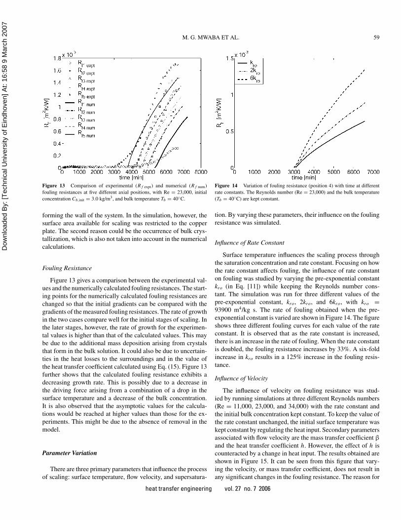
Figure 13 Comparison of experimental (R f expt) and numerical (R f num)fouling resistances at five different axial positions, with Re = 23,000, initialconcentration Cb,init = 3.0 kg/m3, and bulk temperature Tb = 40◦C.

forming the wall of the system. In the simulation, however, thesurface area available for scaling was restricted to the copperplate. The second reason could be the occurrence of bulk crys-tallization, which is also not taken into account in the numericalcalculations.

Fouling Resistance

Figure 13 gives a comparison between the experimental val-ues and the numerically calculated fouling resistances. The start-ing points for the numerically calculated fouling resistances arechanged so that the initial gradients can be compared with thegradients of the measured fouling resistances. The rate of growthin the two cases compare well for the initial stages of scaling. Inthe later stages, however, the rate of growth for the experimen-tal values is higher than that of the calculated values. This maybe due to the additional mass deposition arising from crystalsthat form in the bulk solution. It could also be due to uncertain-ties in the heat losses to the surroundings and in the value ofthe heat transfer coefficient calculated using Eq. (15). Figure 13further shows that the calculated fouling resistance exhibits adecreasing growth rate. This is possibly due to a decrease inthe driving force arising from a combination of a drop in thesurface temperature and a decrease of the bulk concentration.It is also observed that the asymptotic values for the calcula-tions would be reached at higher values than those for the ex-periments. This might be due to the absence of removal in themodel.

Parameter Variation

There are three primary parameters that influence the processof scaling: surface temperature, flow velocity, and supersatura-

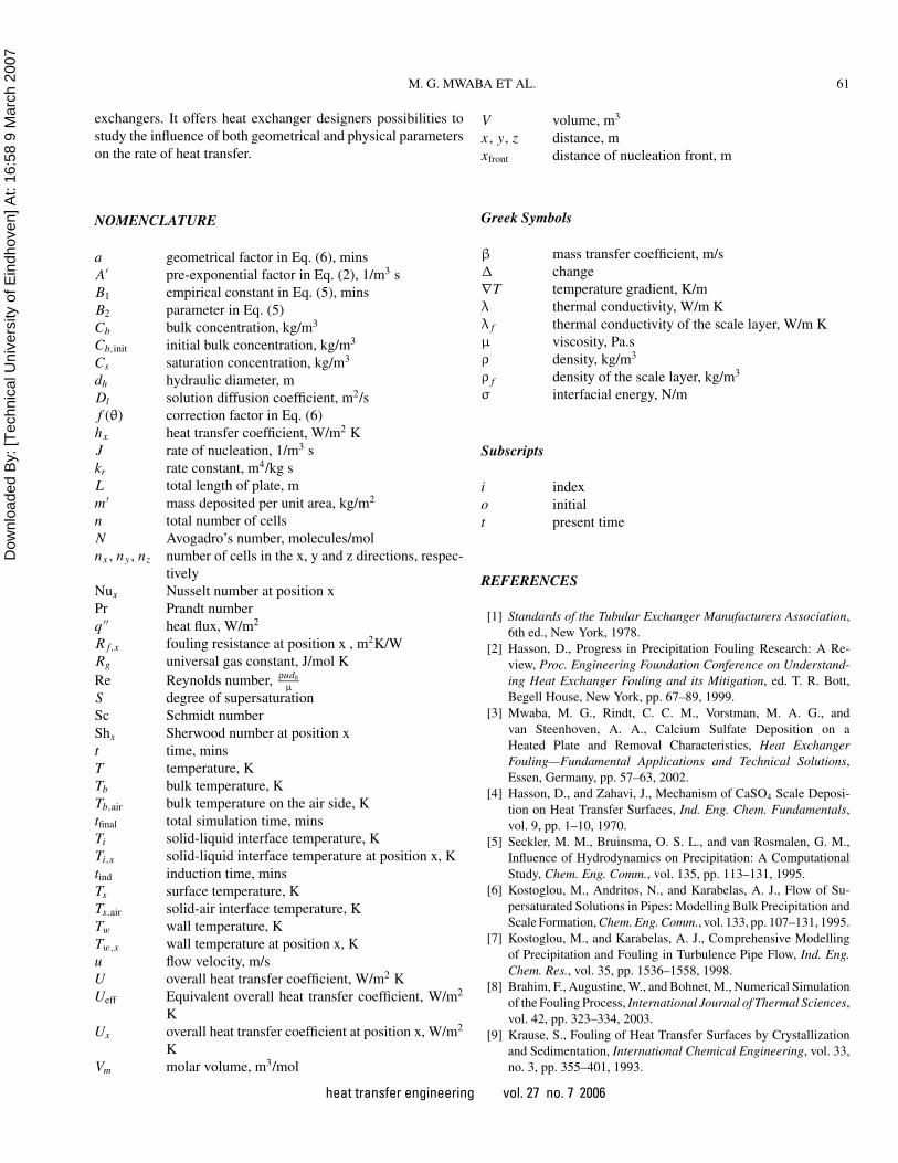
Figure 14 Variation of fouling resistance (position 4) with time at differentrate constants. The Reynolds number (Re = 23,000) and the bulk temperature(Tb = 40◦C) are kept constant.

tion. By varying these parameters, their influence on the foulingresistance was simulated.

Influence of Rate Constant

Surface temperature influences the scaling process throughthe saturation concentration and rate constant. Focusing on howthe rate constant affects fouling, the influence of rate constanton fouling was studied by varying the pre-exponential constantkro (in Eq. [11]) while keeping the Reynolds number cons-tant. The simulation was run for three different values of thepre-exponential constant, kro, 2kro, and 6kro, with kro =93900 m4/kg s. The rate of fouling obtained when the pre-exponential constant is varied are shown in Figure 14. The figureshows three different fouling curves for each value of the rateconstant. It is observed that as the rate constant is increased,there is an increase in the rate of fouling. When the rate constantis doubled, the fouling resistance increases by 33%. A six-foldincrease in kro results in a 125% increase in the fouling resis-tance.

Influence of Velocity

The influence of velocity on fouling resistance was stud-ied by running simulations at three different Reynolds numbers(Re = 11,000, 23,000, and 34,000) with the rate constant andthe initial bulk concentration kept constant. To keep the value ofthe rate constant unchanged, the initial surface temperature waskept constant by regulating the heat input. Secondary parametersassociated with flow velocity are the mass transfer coefficient β

and the heat transfer coefficient h. However, the effect of h iscounteracted by a change in heat input. The results obtained areshown in Figure 15. It can be seen from this figure that vary-ing the velocity, or mass transfer coefficient, does not result inany significant changes in the fouling resistance. The reason for

heat transfer engineering vol. 27 no. 7 2006

Dow

nloa

ded

By: [

Tech

nica

l Uni

vers

ity o

f Ein

dhov

en] A

t: 16

:58

9 M

arch

200

7

60 M. G. MWABA ET AL.

Figure 15 Fouling resistance (position 4) as a function of time at differentReynolds numbers. The rate constant (according to Eq. [11]) and the bulk tem-perature (Tb = 40◦C) are kept constant.

this is that the crystallization process of the salt (CaSO4) usedis controlled by the rate constant rather than the mass transfereffects. An increase of the Reynolds number at a constant heatinput would lead to a decrease in fouling rate due to the loweringof the surface temperature.

Influence of Bulk Concentration

The initial bulk concentration was used as a measure of super-saturation. To study the influence of supersaturation on foulingresistance, the bulk concentration was varied while the veloc-ity remained unchanged. The rate constant was kept constantby maintaining the same initial surface temperature. Maintain-ing the same initial surface temperature distribution also kept the

Figure 16 Fouling resistance as a function of time at different values of bulkconcentration. The rate constant (according to Eq. [11]), the Reynolds number(Re = 23,000), and the bulk temperature (Tb = 40◦C) are kept constant.

saturation concentration constant. Changing the bulk concentra-tion therefore changed the level of supersaturation. The resultsof changing the supersaturation are shown in Figure 16. Shownin this graph are three curves at different values of Cb,init. Theresults show that increasing the level of supersaturation resultsin an increased rate of fouling.

CONCLUSIONS

In this study, the influence of a developing scale layer on heatflow distribution was numerically investigated. A scale layerof CaSO4 was simulated on a copper plate, and the tempera-tures and the surface heat flux were computed. From the resultspresented, it is seen that a developing scale alters the heat fluxdistribution, decreasing the heat flux on areas covered by scale.Further, a scale on top of a heat transfer surface leads to a de-crease in the surface temperature. A comparison of the numeri-cal and experimental results shows very good agreement in theinitial rate of growth.

On the basis of the above, the following conclusions are madefrom this study:

1. The non-uniformity of the heat flux distribution is more pro-nounced when the plate is only partially covered with a scalelayer. This is because the increased thermal resistance due tothe scale layer leads to more heat flowing to areas with lowerthermal resistance.

2. The rate of nucleation increases with an increase in tem-perature, as predicted by Eq. (2). The probability of nucleiforming on areas with higher temperature will be higher. Con-sequently, nuclei form first on the downstream side, and withtime, a nucleation front is seen to move upstream.

3. The surface temperature decreases with an increasing scalethickness and consequently leads to a reduction in the drivingforce for crystallization.

This last conclusion leads to two others:

a. The reduction in the driving force due to a decrease in tem-perature is consistent with the existing crystallization theory[17]. The growth rate depends on the rate constant, which inturn is a function of temperature (see Eq. [11]). Further, forCaSO4, the decrease in temperature increases the saturationconcentration Cs . The combined effect is a reduction in therate of growth.

b. The drop in the interface temperature could also partly ex-plain the asymptotic behavior observed in the experiments[10] at Re = 11,000 and Re = 23,000. As explained ear-lier, removal is not important under these conditions; yet thefouling curves exhibited asymptotic behavior.

In conclusion, it can be said that the numerical modelpresented can be used to investigate CaSO4 fouling in heat

heat transfer engineering vol. 27 no. 7 2006

Dow

nloa

ded

By: [

Tech

nica

l Uni

vers

ity o

f Ein

dhov

en] A

t: 16

:58

9 M

arch

200

7

M. G. MWABA ET AL. 61

exchangers. It offers heat exchanger designers possibilities tostudy the influence of both geometrical and physical parameterson the rate of heat transfer.

NOMENCLATURE

a geometrical factor in Eq. (6), minsA′ pre-exponential factor in Eq. (2), 1/m3 sB1 empirical constant in Eq. (5), minsB2 parameter in Eq. (5)Cb bulk concentration, kg/m3

Cb,init initial bulk concentration, kg/m3

Cs saturation concentration, kg/m3

dh hydraulic diameter, mDl solution diffusion coefficient, m2/sf (θ) correction factor in Eq. (6)hx heat transfer coefficient, W/m2 KJ rate of nucleation, 1/m3 skr rate constant, m4/kg sL total length of plate, mm ′ mass deposited per unit area, kg/m2

n total number of cellsN Avogadro’s number, molecules/molnx , ny , nz number of cells in the x, y and z directions, respec-

tivelyNux Nusselt number at position xPr Prandt numberq ′′ heat flux, W/m2

R f,x fouling resistance at position x , m2K/WRg universal gas constant, J/mol KRe Reynolds number, ρudh

µ

S degree of supersaturationSc Schmidt numberShx Sherwood number at position xt time, minsT temperature, KTb bulk temperature, KTb,air bulk temperature on the air side, Ktfinal total simulation time, minsTi solid-liquid interface temperature, KTi,x solid-liquid interface temperature at position x, Ktind induction time, minsTs surface temperature, KTs,air solid-air interface temperature, KTw wall temperature, KTw,x wall temperature at position x, Ku flow velocity, m/sU overall heat transfer coefficient, W/m2 KUeff Equivalent overall heat transfer coefficient, W/m2

KUx overall heat transfer coefficient at position x, W/m2

KVm molar volume, m3/mol

V volume, m3

x , y, z distance, mxfront distance of nucleation front, m

Greek Symbols

β mass transfer coefficient, m/s� change∇T temperature gradient, K/mλ thermal conductivity, W/m Kλ f thermal conductivity of the scale layer, W/m Kµ viscosity, Pa.sρ density, kg/m3

ρ f density of the scale layer, kg/m3

σ interfacial energy, N/m

Subscripts

i indexo initialt present time

REFERENCES

[1] Standards of the Tubular Exchanger Manufacturers Association,6th ed., New York, 1978.

[2] Hasson, D., Progress in Precipitation Fouling Research: A Re-view, Proc. Engineering Foundation Conference on Understand-ing Heat Exchanger Fouling and its Mitigation, ed. T. R. Bott,Begell House, New York, pp. 67–89, 1999.

[3] Mwaba, M. G., Rindt, C. C. M., Vorstman, M. A. G., andvan Steenhoven, A. A., Calcium Sulfate Deposition on aHeated Plate and Removal Characteristics, Heat ExchangerFouling—Fundamental Applications and Technical Solutions,Essen, Germany, pp. 57–63, 2002.

[4] Hasson, D., and Zahavi, J., Mechanism of CaSO4 Scale Deposi-tion on Heat Transfer Surfaces, Ind. Eng. Chem. Fundamentals,vol. 9, pp. 1–10, 1970.

[5] Seckler, M. M., Bruinsma, O. S. L., and van Rosmalen, G. M.,Influence of Hydrodynamics on Precipitation: A ComputationalStudy, Chem. Eng. Comm., vol. 135, pp. 113–131, 1995.

[6] Kostoglou, M., Andritos, N., and Karabelas, A. J., Flow of Su-persaturated Solutions in Pipes: Modelling Bulk Precipitation andScale Formation, Chem. Eng. Comm., vol. 133, pp. 107–131, 1995.

[7] Kostoglou, M., and Karabelas, A. J., Comprehensive Modellingof Precipitation and Fouling in Turbulence Pipe Flow, Ind. Eng.Chem. Res., vol. 35, pp. 1536–1558, 1998.

[8] Brahim, F., Augustine, W., and Bohnet, M., Numerical Simulationof the Fouling Process, International Journal of Thermal Sciences,vol. 42, pp. 323–334, 2003.

[9] Krause, S., Fouling of Heat Transfer Surfaces by Crystallizationand Sedimentation, International Chemical Engineering, vol. 33,no. 3, pp. 355–401, 1993.

heat transfer engineering vol. 27 no. 7 2006

Dow

nloa

ded

By: [

Tech

nica

l Uni

vers

ity o

f Ein

dhov

en] A

t: 16

:58

9 M

arch

200

7

62 M. G. MWABA ET AL.

[10] Mwaba, M. G., Rindt, C. C. M., Vorstman, M. A. G., and vanSteenhoven, A. A., Experimental Investigation of CaSO4 Crystal-lization on a Flat Plate, Heat Transfer Engineering, vol. 27, no. 3,pp. 42–54, 2006.

[11] Melia, T. P., Crystal Nucleation from Aqueous Solution, J. App.Chem., vol. 15, pp. 345–357, 1965.

[12] Amjad, Z., Calcium Sulfate Dihydrate (Gypsum) Scale Formationon Heat Exchanger Surfaces: The Influence of Scale Inhibitors, J.Colloid and Interface Science, vol. 123, no. 2, pp. 523–536, 1988.

[13] Mahmoud, M. H. H., Rashad, M. M., Ibrahim, I. A., and Abdel-Aal, E. A., Crystal Modification of Calcium Sulfate Dihydrate inthe Presence of Some Surface-Active Agents, Journal of Colloidand Interface Science, vol. 270, pp. 99–105, 2004.

[14] Bohnet, M., Fouling of Heat Transfer Surfaces, Chem. Eng. Tech-nol., vol. 10, pp. 113–125, 1985.

[15] Welty, J. R., Wicks, C. E., Wilson, R. E., and Rorrer, G., Fun-damentals of Momentum, Heat and Mass Transfer, 4th ed., JohnWiley & Sons, New York, 2001.

[16] Versteeg, H. K., and Malalasekera, W., An Introduction to Compu-tational Fluid Dynamics—The Finite Volume Method, Longmann,Essex, England, 1995.

[17] Mullin, J. W., Crystallization, 3rd ed., Butterworth-Heinemann,Oxford, UK, 1993.

Misheck Mwaba obtained his Ph.D. in 2003 fromEindhoven University of Technology, the Nether-lands. He obtained his B.Eng. degree in 1989 from theUniversity of Zambia and his M.Sc. degree in 1992from UMIST, Manchester, UK. His MSc. degree the-sis was on the prediction of stresses in a solidifyingmelt. For his Ph.D., he worked on the problem offouling in industrial heat exchangers, focusing on theproblem of scaling in cane sugar factories. He is cur-

rently working as a Postdoc at Carleton University, Ottawa, Canada. His mainresearch interests are in fouling mitigation and in transport phenomena in HeatPipes and Fuel Cells. He is a member of the American Society of Mechani-cal Engineers (ASME) and the Canadian Society for Mechanical Engineering(CSME).

Camilo Rindt received his M.Sc. and Ph.D. de-grees from Eindhoven University of Technology, theNetherlands. Until the end of 1990, he worked in thefield of biomechanics; since then, he has been a lec-turer on thermal transport phenomena in the field ofenergy technology. His main research interests are inthe fields of conjugate heat transfer, radiation mod-eling, and fouling of heat exchangers. Regarding thelatter topic, he is focusing on the fouling problemsin waste incinerators and sugar plants.

Anton van Steenhoven is a professor of Energy Tech-nology at the Department of Mechanical Engineer-ing at the Eindhoven University of Technology, theNetherlands. He gained his Ph.D. in 1979 on a the-sis about fluid mechanics of heart valves. His currentresearch interests are the numerical and experimentalanalysis of fluid flow and heat transfer and its appli-cation to the design of energy equipment.

Marius Vorstman is an assistant professor in theProcess Development Group of the Department ofChemical Engineering at the Eindhoven Universityof Technology, the Netherlands. He graduated fromthe same university in 1965. His research interests arein crystallization and separation technology.

heat transfer engineering vol. 27 no. 7 2006