Processes of carbonate precipitation in modern microbial mats
Upload
khangminh22Category
view
5download
0
PRECIPITATION OF CALCIUM CARBONATE
AND ITS IMPACT ON
HEAT EXCHANGERS OF COOLING WATER SYSTEMS
BY
CHENG HOONG KUO
B.Sc. (Hons), Singapore, M.App.Sc., Australia
A thesis submitted to the University of New South Wales
for the degree of
Doctor of Philosophy
November, 1984
SR.P.T10
CERTIFICATE OF ORIGINALITY
I hereby declare that this thesis is my own work and that, to the best of my knowledge and belief, it contains no material previously published or written by another person nor material which to a substantial extent has been accepted for the award of any other degree or diploma of a university or other institute of higher learning, except where due acknowledgement is made in the text of the thesis.
UNIVERSITY OF N.S.W.
4 DEC 1985
LIBRARY
This thesis has not been previously presented
in whole or part, to any University or Instituition for
higher degree.
CHENG HOONG KUONovember, 1984

Dedicated to
MY WIFE
i
fUuiyll.d ^ JABSTRACT
The solubility of calcium carbonate decreases with increasing
temperature. It can therefore precipitate in cooling water systems, causing a loss of thermal efficiency. In order to be relevant to cooling water systems, the calcium carbonate precipitation was studied in an unseeded batch stirred reactor. All three crystallogra
phic forms of calcium carbonate (calcite, aragonite and vaterite) were observed in the experiments covering a wide range of degrees of supersaturation, stirring speeds and temperatures. The interfacial energies of calcite and vaterite were calculated. An empirical expression for secondary nucleation incorporating power was derived.The mechanism of crystallization was established as surface-reaction controlled and the kinetics expressed by the Davies and Jones equation. This led to the calculation of overall growth rate constants of calcite and vaterite.
Scaling in the heat exchangers was studied at pilot plant scale
by a test rig constructed to model the Lake Liddell power station cooling water system. The threshold Langelier Index for scaling to occur was found to be 1.40 and 1.25 with ion pair consideration. This indicates that the traditional +1.0 Langelier Index recommended for power station cooling water practice is justified. The threshold Langelier Index calculated at the heat transfer surface temperature was 1.69 and
1.52 with ion pair consideration. This successfully correlated with
literature data and that generated at Wallerawang power station.
ii
Scaling was found to be completely prevented due to high velocity shear stress especially when the threshold Langelier Index based on surface temperature was moderately exceeded. From the precipitation study, the formation of discrete aragonite at 35°C and beyond
also explained the fact that higher threshold Langelier Indexes were tolerable. The overall growth rate model based on the concept of the
surface-controlled mechanism used to derive crystallization kinetics in the precipitation study was developed to predict the scaling rate. When combined with the Hasson's diffusion model, the former overesti
mated the scaling rate whereas the latter underestimated the scaling rate. The failure to incorporate the actual reaction/mass transfer surface area in both models was considered to be critical.
i
ABSTRACT
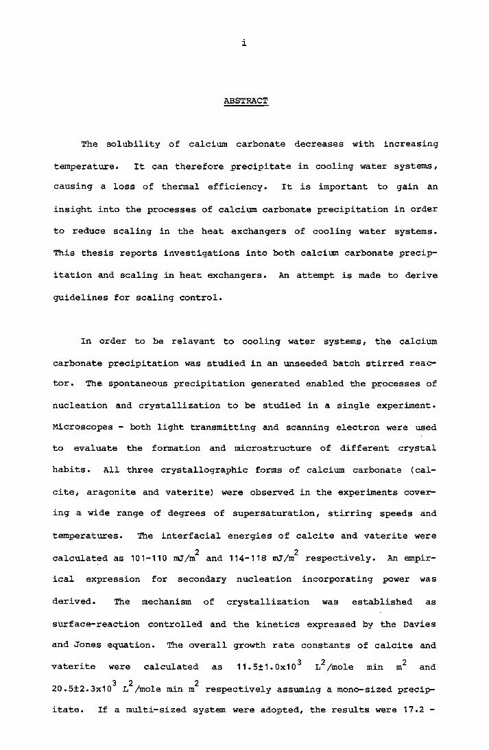
The solubility of calcium carbonate decreases with increasing
temperature. It can therefore precipitate in cooling water systems, causing a loss of thermal efficiency. It is important to gain an
insight into the processes of calcium carbonate precipitation in order to reduce scaling in the heat exchangers of cooling water systems. This thesis reports investigations into both calcium carbonate precip
itation and scaling in heat exchangers. An attempt is made to derive
guidelines for scaling control.
In order to be relavant to cooling water systems, the calcium carbonate precipitation was studied in an unseeded batch stirred reactor. The spontaneous precipitation generated enabled the processes of nucleation and crystallization to be studied in a single experiment. Microscopes - both light transmitting and scanning electron were used to evaluate the formation and microstructure of different crystal habits. All three crystallographic forms of calcium carbonate (cal-
cite, aragonite and vaterite) were observed in the experiments covering a wide range of degrees of supersaturation, stirring speeds and
temperatures. The interfacial energies of calcite and vaterite were2 2calculated as 101-110 rrvJ/m and 114-118 rtvJ/m respectively. An empir
ical expression for secondary nucleation incorporating power was
derived. The mechanism of crystallization was established as
surface-reaction controlled and the kinetics expressed by the Daviesand Jones equation. The overall growth rate constants of calcite and
. 3 2 2vaterite were calculated as 11.5±1.0x10 L /mole min m and3 2 220.5±2.3x10 L /mole min m respectively assuming a mono-sized precip
itate. If a multi-sized system were adopted, the results were 17.2 -
ii
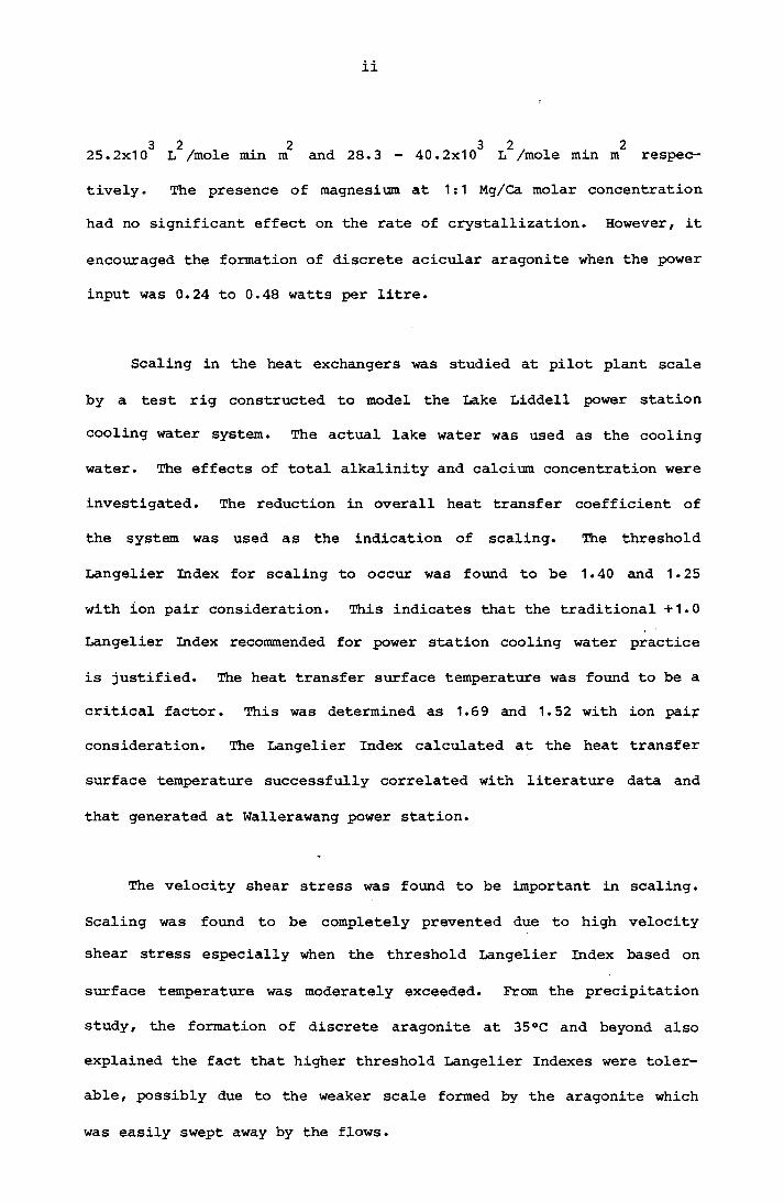
25.2x10 L /mole min m and 28.3 - 40.2x10 L /mole min m respec
tively. The presence of magnesium at 1:1 Mg/Ca molar concentration
had no significant effect on the rate of crystallization. However, it
encouraged the formation of discrete acicular aragonite when the power
input was 0.24 to 0.48 watts per litre.
Scaling in the heat exchangers was studied at pilot plant scale
by a test rig constructed to model the Lake Liddell power station
cooling water system. The actual lake water was used as the cooling
water. The effects of total alkalinity and calcium concentration were
investigated. The reduction in overall heat transfer coefficient of
the system was used as the indication of scaling. The threshold
Langelier Index for scaling to occur was found to be 1.40 and 1.25
with ion pair consideration. This indicates that the traditional +1.0 Langelier Index recommended for power station cooling water practice
is justified. The heat transfer surface temperature was found to be a
critical factor. This was determined as 1.69 and 1.52 with ion pair
consideration. The Langelier Index calculated at the heat transfer
surface temperature successfully correlated with literature data and
that generated at Wallerawang power station.
The velocity shear stress was found to be important in scaling.
Scaling was found to be completely prevented due to high velocity shear stress especially when the threshold Langelier Index based on
surface temperature was moderately exceeded. From the precipitation
study, the formation of discrete aragonite at 35°C and beyond also
explained the fact that higher threshold Langelier Indexes were toler
able, possibly due to the weaker scale formed by the aragonite which
was easily swept away by the flows.
iii
The overall growth rate model based on the concept of the
surface-controlled mechanism used to derive crystallization kinetics
in the precipitation study was developed to predict the scaling rate.
When combined with the Hasson's diffusion model, the former overes
timated the scaling rate whereas the latter underestimated the scaling
rate. The failure to incorporate the actual reaction/mass transfer surface area in both models was considered to be critical.

iv
ACKNOWLEDGEMENTSI would like to express my sincere appreciation to my supervisor,
A/Prof. D. Barnes, for his constant support, enthusiasm and guidance;
my co-supervisor, Mr. P.J. Bliss, for his encouragement and understanding throughout this study;
The Electricity Commission of New South Wales, for the provision of the University Scholarship to carry out this project;
Mr. A.G. Willard of the School of Mining Engineering for the use of the Microvideomat 2 Image Analyzer;Dr. V.N.E. Robinson of the School of Textile Technology for the use of the Scanning Electron Microscope.
I would also like to express my sincere thanks to many of the technical staff at the School of Civil Engineering. Their assistance during various crucial periods of the project have proved to be most invaluable.
Special thanks also go to Caroline Loong, Ching Long Lim and Edward
Tang for their efforts in preparing the final copy of this thesis.
Finally, my deepest appreciation goes to my wife, who has always been the source of my strength and perseverance.
V
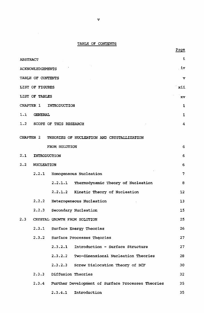
TABLE OF CONTENTSPage
ABSTRACT 1
ACKNOWLEDGEMENTS ivTABLE OF CONTENTS V
LIST OF FIGURES xiiLIST OF TABLES xvCHAPTER 1 INTRODUCTION 11.1 GENERAL 11.2 SCOPE OF THIS RESEARCH 4
CHAPTER 2 THEORIES OF NUCLEATION AND CRYSTALLIZATIONFROM SOLUTION 6
2.1 INTRODUCTION 62.2 NUCLEATION 6
2.2.1 Homogeneous Nucleation 72.2.1.1 Thermodynamic Theory of Nucleation 82.2.1.2 Kinetic Theory of Nucleation 12
2.2.2 Heterogeneous Nucleation 132.2.3 Secondary Nucleation 15
2.3 CRYSTAL GROWTH FROM SOLUTION 252.3.1 Surface Energy Theories 262.3.2 Surface Processes Theories 27
2.3.2.1 Introduction - Surface Structure 272.3.2.2 Two-dimensional Nucleation Theories 282.3.2.3 Screw Dislocation Theory of BCF 30
2.3.3 Diffusion Theories 322.3.4 Further Development of Surface Processes Theories 35
2.3.4.1 Introduction 35
vi
Page
2.3.4.2 Surface Reaction Models of Doremus 352.3.4.3 Surface Adsorption Model of Walton 372.3.4.4 Davies and Jones Double-layer Model 38
2.3.4.5 Surface Reaction Model of Konak 392.3.4.6 Nielsen Electrolyte Crystal Growth Theory 41
2.4 CONCLUSIONS FOR CHAPTER 2
CHAPTER 3 WATER CHEMISTRY OF CALCIUM CARBONATE/COMPUTER PROGRAMMESFOR CHEMICAL COMPOSITION CALCULATIONS 44
3.1 BASIC CHEMISTRY OF CALCIUM CARBONATE IN AQUEOUS SYSTEM 44
3.1.1 Introduction 443.1.2 Carbonate Species Distribution in a Closed System 45
3.1.3 Carbonate Species Distribution in an Open System 473.1.4 Ion Pairs Consideration 483.1.5 Ionic Strength Consideration 493.1.6 Temperature Consideration 503.1.7 Calcium Carbonate Solubility in a Given Aqueous Matrix 52
3.2 COMPUTER PROGRAMMES 553.2.1 Programmes for Chemical Composition Calculation 55
3.2.1.1 Pure Calcium Carbonate System (PROG-CS) 553.2.1.2 Calcium Carbonate in the Presence of
Magnesium (PROG-CMS) 56
3.2.1.3 Calcium Carbonate in the Presence of Magnesium and Sulphate - Lake Liddell
WATER (PROG-CMSS) 563.2.2 Programmes for Precipitation Calculation 57
3.2.2.1 Pure Calcium Carbonate System (PROG-PCS) 57
3.2.2.2 Calcium Carbonate in the Presence ofMagnesium (PROG-PCMS) 59
vii
PageCHAPTER 4 EXPERIMENTAL STUDIES OF PRECIPITATION OF
CALCIUM CARBONATE 60
4.1 NUCLEATION AND CRYSTALLIZATION OF CALCIUM CARBONATE -A LITERATURE REVIEW 604.1.1 Introduction 614.1.2 Nucleation of Calcium Carbonate 61
4.1.3 Crystallization of Calcium Carbonate 664.2 EXPERIMENTAL METHOD - A GENERAL SURVEY 79
4.2.1 Nucleation Studies 794.2.1.1 * Homogeneous Nucleation Studies 794.2.1.2 Metastable Zone Width 824.2.1.3 Induction Period Method 84
4.2.2 Crystallization Studies 864.2.2.1 Conventional Methods 864.2.2.2 Population Balance by MSMPR Crystallizer 88
4.3 INTERPRETATION OF DESUPERSATURATION CURVE 924.3.1 Chronomal Analysis 934.3.2 Turnbull's Characteristic Curve 964.3.3 Size Distribution Consideration 974.3.4 Overall Growth Rate (Simplified) 1014.3.5 Overall Growth Rate with Size Consideration 104
4.4 EXPERIMENTAL 1064.4.1 Introduction 1064.4.2 Equipment 1074.4.3 Procedures 110
4.4.3.1 Batch Stirred Reactor Crystallization
Experiments 1104.4.3.2 Microscopic Observation and Crystal
Number Count 112
viii
Page4.4.3.3 Crystal Size Measurement 113
4.5 RESULTS 1144.5.1 Primary Nucleation of Calcium Carbonate Precipitation 114
4.5.1.1 Experiments at Constant Stirring Speed 114
4.5.1.2 Experiments at Different Stirring Speed 115
4.5.1.3 Experiments at Different Stirring Speedof 1:1 Mg/Ca Molar Concentration 115
4.5.2 Secondary Nucleation of Calcium CarbonatePrecipitation 1154.5.2.1 The Calculation of Power Input in a
Stirred Reactor 1164.5.2.2 Experiments of Pure Calcium Carbonate
System 1194.5.2.3 Experiments on 1:1 Mg/Ca Molar Concentration 119
4.5.3 Crystallization of Calcium Carbonate Precipitation 1204.5.3.1 Bulk Crystallization of Pure Calcium
Carbonate System 1204.5.3.2 Bulk Crystallization of Calcium
*
Carbonate in 1:1 Mg/Ca Molar Concentration 122
CHAPTER 5 DISCUSSION OF CALCIUM CARBONATE PRECIPITATION STUDIES 1235.1 NUCLEATION OF CALCIUM CARBONATE 123
5.1.1 General 123
5.1.2 Visual Induction Period Data 1235.1.3 Latent Period Data 1285.1.4 An Explanation for the Formation of Different
Crystallographic Forms of Calcium Carbonate 1325.1.5 Secondary Nucleation of Pure Calcium Carbonate
System 134

ix
5.1.6 Secondary Nucleation of 1:1 Mg/Ca MolarPage
Concentration System 1395.2 CRYSTALLIZATION OF CALCIUM CARBONATE 139
5.2.1 Crystal Surface and Volume Shape Factors 1425.2.2 Overall Growth Rate of Crystallization of Pure
Calcium Carbonate System 1445.2.3 Formation of Different Crystal Habits in Pure
Calcium Carbonate System 1545.2.4 The Effect of Magnesium in Calcium Carbonate
Bulk Crystallization 156
CHAPTER 6 CALCIUM CARBONATE SCALING IN HEAT EXCHANGERS 1586.1 INTRODUCTION 1586.2 MATHEMATICAL MODELS OF FOULING 160
6.2.1 Rate of Deposition 1616.2.1.1 Driving Force 1626.2.1.2 Kinetic 162
6.2.2 Rate of Removal 1636.3 FACTORS AFFECTING SCALING 165
6.3.1 Velocity 1656.3.2 Temperature 1666.3.3 Tube Surface 1666.3.4 Water Chemistry 167
6.4 CALCIUM CARBONATE SATURATION INDEXES 1676.4.1 Langelier Index (LI) 1686.4.2 Ryznar Stability Index (RI) 1706.4.3 Driving Force Factor (DFI) 1706.4.4 Aggressiveness Index (AI) 1716.4.5 Momentary Excess (ME) 1716.4.6 Calcium Carbonate Precipitation Potential 172
X
Page6.4.7 Comparison of Indexes 174
6.5 LITERATURE REVIEW ON CALCIUM CARBONATE SCALING(PRECIPITATION FOULING) 175
6.6 CONCLUSIONS OF CHAPTER 6 190
CHAPTER 7 INVESTIGATION OF SCALING POTENTIAL OF LAKE LIDDELLWATER TO POWER STATION CONDENSER TUBES 192
7.1 INTRODUCTION 192
7.2 EXPERIMENTAL 1947.2.1 Experimental Design 1947.2.2 Experimental Apparatus 195
7.2.2.1 Heating System 1951.2.2.2 Cooling System 197
7.2.3 Experimental Procedure 198
7.3 RESULTS AND DISCUSSION 2007.3.1 Methyl Orange Alkalinity Experiments 2007.3.2 Calcium Hardness Experiments 2017.3.3 Threshold Langelier Index Calculated based on
Bulk Inlet Temperature 2027.3.4 Threshold Langelier Index Calculated based on
Heat Transfer Surface Temperature 205
7.4 CONCLUSIONS 211
CHAPTER 8 PREDICTION OF CALCIUM CARBONATE SCALING IN THE HEATEXCHANGER OF A COOLING WATER SYSTEM 212
»
8.1 INTRODUCTION 2128.2 CALCULATION OF CALCIUM CARBONATE SCALING RATE IN THE
HEAT EXCHANGER 2138.3 SOME INVESTIGATION ON CALCIUM CARBONATE SCALING REPORTED
IN THE LITERATURE 216
xi
Page8.3.1 Morse and Knudsen 2168.3.2 Coates and Knudsen 218
8.3.3 Watkinson 219
8.4 COMPARISON OF CALCULATED AND EXPERIMENTALLY MEASURED
SCALING RATE 2218.5 EFFECT OF SURFACE TEMPERATURE AND VELOCITY 225
8.6 WALLERAWANG POWER STATION - ELECTRICITY COMMISSION OFNEW SOUTH WALES 229
8.7 EFFECT OF MAGNESIUM 233
CHAPTER 9 CONCLUSIONS AND RECOMMENDATIONS 2369.1 CONCLUSIONS 2369.2 RECOMMENDATIONS 245
NOTATION 249APPENDIX A RESULTS OF SPONTANEOUS CRYSTALLIZATION EXPERIMENTS 258APPENDIX B PHOTOMICROGRAPHS OF CRYSTALS FROM SPONTANEOUS
CRYSTALLIZATION EXPERIMENTS 288APPENDIX C GRAPHS OF SPONTANEOUS CRYSTALLIZATION EXPERIMENTS
- THE CALCULATION OF THE OVERALL GROWTH RATE CONSTANTS 297
APPENDIX D RESULTS OF FINAL CRYSTAL SIZE MEASUREMENT 331APPENDIX E COMPOSITION OF SCALE 341APPENDIX F LISTINGS OF PROGRAMMES 364
LIST OF REFERENCES 379
FIGURE2-1
2-2
3- 1
4- 1 4-2
4-3
4- 45- 1 5-2
5-3
5-4
5-5
5-6
5-7
5-8
5-9a
xii
LIST OF FIGURES
Surface Energies at the Boundaries Between Three
Phases (Two Solids, One Liquid)Surface Structure of CrystalDistribution of Carbonic Species with pH for
-31.0x10 M Total Carbonic Concentration A Typical Desupersaturation Curve Schematic Representation of the Apparatus for
CaCO^ Precipitation StudyCross-sectional View of the Stirred ReactorSchematic Representation of Geometry A and Geometry B
-2 -3The Plot of LOG Induction Period Against (LOG S) T The Plot of LOG 0^ Against LOG a Using Data from Geometry A, 220 r.p.m. Experiments at 25°C The Plot of Reciprocal of Induction Period Against Degree of Supersaturation using Data from Geometry A, 220 r.p.m. Experiments at 25°C
-2The Plot of LOG 0 Against (LOG S) using Dataidtfrom the Homogeneous Nucleation Region at 25°C
The Plot of Induction Period Against Power Input
for S = 57 - 63 at 25°CThe Plot of Latent Period Against Power Input for
S = 57 - 63 at 25°CThe Plot of Induction Period Against Power Input
for 1:1 Mg/Ca System (S = 24) at 25°CThe Plot of Latent Period Against Power Input
for 1:1 Mg/Ca System (S = 24) at 25°CThe Final Number of Crystals per Litre at Different
Page
13a
27a
47a
92a
108a108b108c123a
128a
128b
130a
131a
131b
132a
132a
Stirring Speed at 25°C (S = 57 - 63) 134a
xiii
FIGURE Page
5-9b The Final Number of Crystals per Litre at Different
Stirring Speed at 25°C 134a5-10 The Number of Crystals Counted with respect to
Time for Experiment PE21 (220 r.p.m., Geometry A) 135a5-11 The Linear Relationship of Secondary Nucleation Rate
with respect to Power Input for S = 57 -63 at 25°C 136a5-12 Empirical Correlation of Secondary Nucleation Rate
of Calcium Carbonate at 25°C in a Batch Stirred
Reactor 137a5-13 The Number of Crystal Counted with respect to Time
for Experiment PE19 (400 r.p.m., Geometry B) 139a5-14 Schematic Representation of Rhombohedral Calcite 143a7-1 Schematic Representation of Test Rig 195a7-2 Gibault Fittings and Removable Condenser Tube 196a7-3 Change of Overall Heat Transfer Coefficient with
Time, Expt. 4 201a7-4 Change of Overall Heat Transfer Coefficient with
Time, Expt. 8 201b✓7-5 Change of Overall Heat Transfer Coefficient with
Time, Expt. 11 201c7-6 Change of Overall Heat Transfer Coefficient with
Time, Expt. 12 201d7-7 Change of Overall Heat Transfer Coefficient with
Time, Expt. 13 201e7-8 Change of Overall Heat Transfer Coefficient with
Time, Expt. 14 201f7-9 Langelier Index According to Larson and Buswell
at Bulk Inlet Temperature 203a7-10 Langelier Index with Ion Pair Consideration at
Bulk Inlet Temperature 203b
xiv
FIGURE Page7-11 Langelier Index According to Larson and
Buswell at Surface Temperature 209a
7- 12 Langelier Index with Ion Pair Consideration at
Surface Temperature 209b
8- 1 Schematic Representation of the CaCO^ Scalingon a Heat Transfer Surface 214
8-2 Comparison of Measured and Predicted ScalingRate by Overall Growth Rate Model 221a
8-3 Comparison of Measured and Predicted Scaling Rateby Hasson's Ionic Model 221b

XV
LIST OF TABLESTABLE Page4-1 Values of Interfacial Energies Obtained for
each Variety of Calcium Carbonate 624-2 Induction and Latent Period of Calcium Carbonate
Nucleation Determined in Geometry A Stirred Reactor at 220 r.p.m. 114a
4-3 Calculation of Results for Calcium CarbonateInduction and Latent Period Determined in Geometry A Stirred Reactor 114b
4-4 Induction and Latent Period of Calcium CarbonateNucleation in Geometry B Reactor at 25°C under Different Stirring Speed and Supersaturation 115a
4-5 Calculation of Results for Calcium Carbonate Inductionand Latent Period Determined in Geometry B Stirred Reactor 115b
4-6 Induction and Latent Period of Calcium CarbonateNucleation of S = 24 Determined in Geometry B Reactor
with 1:1 Mg/Ca Molar Ratio at 25°C 115c4-7 Secondary Nucleation of Calcium Carbonate at 25°C 119a4-8 Secondary Nucleation of Calcium Carbonate in 1:1
Mg/Ca Molar Concentration System at 25°C 120a
4-9 Bulk Crystallization of Calcium Carbonate at Various* Temperatures at 220 r.p.m. (0.3218 J/L s) Stirring
Speed in Geometry A 120b4-10 Bulk Crystallization of Calcium Carbonate at 25°C at
Various Stirring Speeds (Simplified) 121a4-11 Bulk Crystallization of Calcium Carbonate at 25°C at
Various Stirring Speed (Size Consideration) 121b
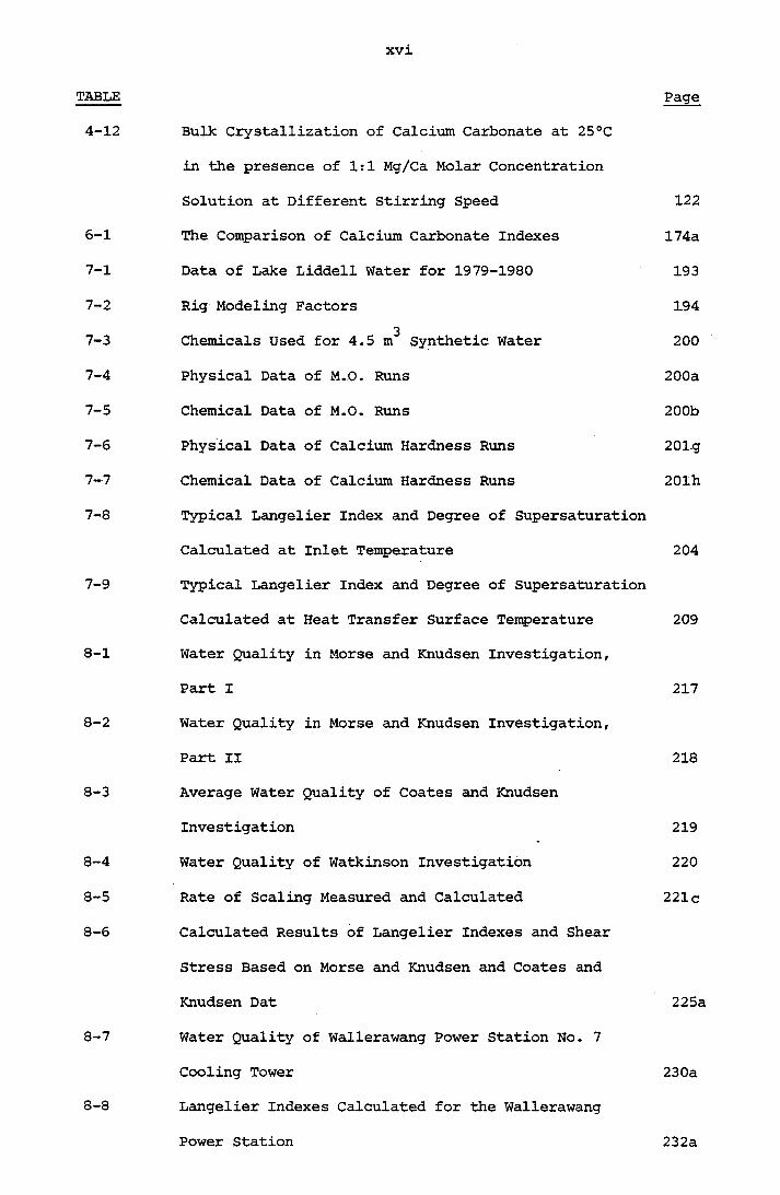
TABLE Page4-12 Bulk Crystallization of Calcium Carbonate at 25°C
in the presence of 1:1 Mg/Ca Molar Concentration Solution at Different Stirring Speed 122
6- 1 The Comparison of Calcium Carbonate Indexes 174a
7- 1 Data of Lake Liddell Water for 1979-1980 1937-2 Rig Modeling Factors 194
37-3 Chemicals Used for 4.5 m Synthetic Water 200
7-4 Physical Data of M.O. Runs 200a7-5 Chemical Data of M.O. Runs 200b7-6 Physical Data of Calcium Hardness Runs 201g7-7 Chemical Data of Calcium Hardness Runs 201h7-8 Typical Langelier Index and Degree of Supersaturation
Calculated at Inlet Temperature 2047- 9 Typical Langelier Index and Degree of Supersaturation
Calculated at Heat Transfer Surface Temperature 2098- 1 Water Quality in Morse and Knudsen Investigation,
Part I 2178-2 Water Quality in Morse and Knudsen Investigation,
Part II 2188-3 Average Water Quality of Coates and Knudsen
Investigation 2198-4 Water Quality of Watkinson Investigation 220
8-5 Rate of Scaling Measured and Calculated 221c8-6 Calculated Results of Langelier Indexes and Shear
Stress Based on Morse and Knudsen and Coates and Knudsen Dat 225a
8-7 Water Quality of Wallerawang Power Station No. 7Cooling Tower 230a
8-8 Langelier Indexes Calculated for the WallerawangPower Station 232a

1
CHAPTER 1
INTRODUCTION
1.1 GENERAL
Calcium carbonate is the major constituent of limestones, mar
bles, chalks, oyster shells, and corals. It is a white powder that is
insoluble in water but becomes soluble in the presence of carbon diox
ide. Natural water containing dissolved calcium carbonate is called
'hard' water. Calcium carbonate obtained from natural sources is used
as a filler for various products, such as ceramics and glass, and as
starting material for the production of calcium oxide.
Calcium carbonate is also prepared synthetically by passing car
bon dioxide gas through milk of lime (calcium hydroxide) or by combin
ing solutions of calcium chloride and sodium carbonate. The product
is called 'precipitated' calcium carbonate and is used when high pur
ity is required. For example in medicine (antacid and dietary calcium
supplement), in food (baking powder), and in laboratory chemical syn
thesis. Pure calcium carbonate has a specific gravity ranging from
2.70 to 2.93 and decomposes when heated to about 825°C.
There are five known polymorphs of calcium carbonate (Encyclo
pedia Britannica, 1984), namely calcite, aragonite, vaterite, calcite
II and calcite III. Calcite II and calcite III are only found in the
laboratory under pressures of the order of 20,000 atm. at room
2
temperature. The commonest polymorph of calcium carbonate in nature
is calcite, while aragonite is the next most common and vaterite is
comparatively rare.
Calcium carbonate will precipitate out from solution if it
exceeds its solubility product. The crystallographic forms of calcium
carbonate are dependent on the condition of precipitation. Although
calcium carbonate precipitates in nature to form stalactites and
stalagmites in limestone caves, their precipitation in heat exchangers
and water transmitting pipelines is an unwanted phenomenon. The pre
cipitation of calcium carbonate in the heat exchangers also known as
precipitation fouling or more commonly, scaling, will significantly
reduce the design heat transfer capacity because of the poor heat con
ductivity of the calcium carbonate deposit on the heat transfer surfaces .
Scaling of the heat exchangers is commonly encountered in the
cooling water systems. There are three types of cooling water systems.
1. Once-through systems, in which the water is discharged, after
use, usually to the source from which it was originally with
drawn .
2. Open recirculating systems, in which the water is used repeat
edly. The heat picked up by the water during the passage through
the heat exchangers is dissipitated by direct contact with atmos
pheric air in the evaporative cooling device such as a cooling
pond, a spray pond, or a cooling tower.
3. Closed recirculating systems, in which the water is also used
repeatedly but the heat which is picked up is removed by some
3
form of heat exchanger where there is no direct contact between
the water and the coolent. The typical examples of such systems
are the cooling systems of diesel and other internal combustion
engines.
The closed recirculating systems are generally more susceptible to
corrosion because they are often made up of a number of dissimilar
metals in contact and consequently increase the risk of corrosion.
Both once-through and open recirculating systems are widely used in
the large scale practice. The heat exchangers of these systems are
susceptible to both scaling as well as corrosion depending on the
quality of the water. The indexes to indicate the corrosivity and
scale-forming potential of the water will be discussed in Chapter 6.
Calcium carbonate is a natural constituent of water. Unfortunately
its solubility is inversely proportional to temperature. This makes
the hot surfaces of the heat exchangers more susceptible to calcium
carbonate precipitation due to local temperature gradients. The
increase in concentration in the open recirculating systems due to
evaporation also increases the risk of scaling. The current state of
art to deal with calcium carbonate scaling in heat exchangers consists
of two areas of management. Firstly, the heat exchangers are designed
to incorporate a safety factor called a fouling factor caused by the
calcium carbonate deposit. Secondly, the cooling water system will be
operating with some forms of treatment and monitoring programme to
avoid calcium carbonate precipitation in the heat exchangers. In the
first instance, the capital installation cost is increased because of
the fouling factor incorporated. It was estimated in United Kingdom
that in 1977 the extra capital cost on heat exchangers attributed to
all forms of fouling was approximately 40 million pounds (Thackery,

4
1979). If the ancilliary items such as boilers, water treatment
plants etc. were included, the approximate total was 100 millions
pounds. Obviously, the cooling water management has already generated
on entire industry to keep the heat exchangers clean. The problem of
heat exchangers fouling is a very real one. Because of the huge extra
capital cost involved in catering for large heat transfer surface, the
choice of fouling factor has to be realistic. However, this requires
a better understanding of fouling mechanisms involved in each type of
fouling. In the case of fouling in water cooling systems, the fouling
due to calcium carbonate precipitation is the most widely reported.
The precipitation of calcium carbonate is the obvious starting
point to achieve a better understanding of calcium carbonate scaling
in heat exchangers. The detailed study of such a process falls into
the areas of chemical nucleation and crystallization of inorganic
salts from the solution.
1.2 SCOPE OF THIS RESEARCH
This study was initiated to provide information on the mechanism
of calcium carbonate precipitation and the control of the precipita
tion in full scale plants. The following are the areas of this
research:
1 . To investigate the bulk nucleation of calcium carbonate in the
solution.
2. To investigate the bulk nucleation of calcium carbonate in the
presence of magnesium.3. To investigate the effect of mechanical power absorbed by the
5
solution to the precipitation of calcium carbonate.
4. To investigate the kinetics of calcium carbonate bulk crystalli
zation in pure calcium system as well as in the presence of mag
nesium.
5. To investigate the scale-forming potential of Lake Liddell water
used for Liddell power station cooling water system.
6. To establish a threshold of scaling for Liddell power station
cooling water system as indicated by Langelier Index and con
trolled by dosing sulphuric acid into the cooling pond (Lake Lid
dell) .
7. To test the general applicability of such a scaling threshold
represented by the Langelier Index on cooling water systems.
8. To apply the kinetics of calcium carbonate bulk precipitation in
explaining and predicting the rate of scaling in the heat
exchangers of the cooling water systems.
6
CHAPTER 2
THEORIES OF NUCLEATION AND CRYSTALLIZATION FROM SOLUTION
2.1 INTRODUCTION
Although crystallization is a common phenomenon observed, a
detailed understanding of the mechanism is still limited. In the
chemical industry where crystallization processes are exploited to
produce chemicals, it is still as much an art as a science. Crystall
ization is generally considered to take place in three stages: nuclea-
tion, growth and recrystallization (Buckley, 1951; Van Hook, 1961;
Nielsen, 1964; Strickland-Constable, 1968; Mullin, 1972). Recrystall
ization is sometimes further classified into ripening and recrystalli
zation (ageing) (Lieser, 1969). Nevertheless, the above classifica
tion of crystallization is only a convenient description of the process because the various steps overlap dur»ing the crystallization pro
cess .
2.2 NUCLEATION
In order for crystallization to occur, firstly the dissolved sub
stance in the solution must be supersaturated. Secondly there must be
centres of crystallization, seeds, embryos or nuclei present in the
solution. Nucleation is the process of phase transformation of dis
solved substances (ions or molecules) into submicroscopic particles.
Nucleation can be either homogeneous (spontaneous) or heterogeneous.
7
Homogeneous nucleation can only occur due to the availability of suf
ficient chemical potential, namely supersaturation. The dissolved ions or molecules combine together to form clusters. Heterogeneous
nucleation takes place on small particles of foreign matter (seeds) on which ions or molecules are deposited (eg. by adsorption) until a
nucleus has been formed. These types of nucleation are also known as primary nucleation. On the other hand, nuclei are always generated in
the vicinity of crystals present in a supersaturated system. This phenomenon is known as secondary nucleation.
2.2.1 Homogeneous Nucleation
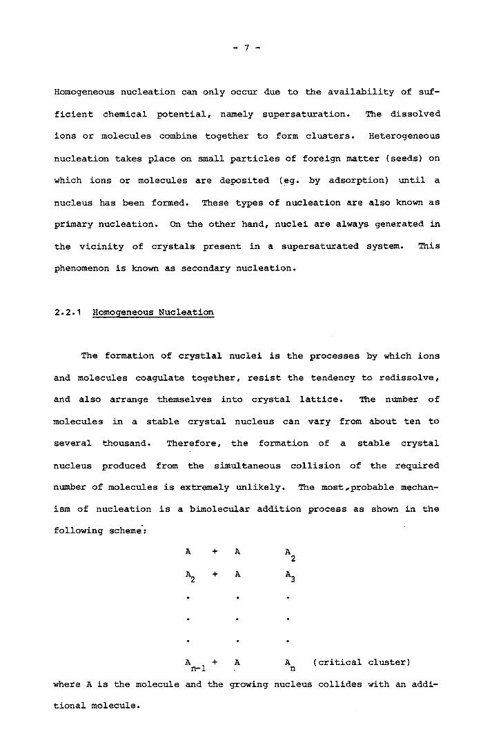
The formation of crystlal nuclei is the processes by which ions and molecules coagulate together, resist the tendency to redissolve, and also arrange themselves into crystal lattice. The number of molecules in a stable crystal nucleus can vary from about ten to several thousand. Therefore, the formation of a stable crystal
nucleus produced from the simultaneous collision of the required number of molecules is extremely unlikely. The most,, probable mechanism of nucleation is a bimolecular addition process as shown in the following scheme:
A + A A2
A +n-1where A is the molecule and the
A A (critical cluster)ngrowing nucleus collides with an addi
tional molecule.
8
The nature of the critical cluster (nucleus) is still not cer
tain. They could be miniature crystals or could be a structure
without a clearly defined surface (Christiansen, 1954; Khamskii, 1969;
Mullin, 1972). The size of nuclei and the short existence of nuclei
in the crystallization process present both theoretical and practical
difficulties to the study of this phenomenon. Nevertheless, some
attempts have been made to describe this phenomenon using both thermo
dynamic and kinetic approaches.
2.2. 1. 1 Thermodynamic Theory of Nucleation
The classical theory of nucleation is derived from the work of
Gibbs (1928), Volmer (1939), Becker and Doring (1935) and is based on
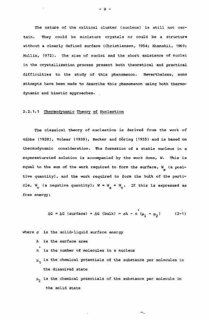
thermodynamic consideration. The formation of a stable nucleus in a
supersaturated solution is accompanied by the work done, W. This is
equal to the sum of the work required to form the surface, W (a posi-stive quantity) , and the work required to form the bulk of the parti
cle, (a negative quantity); W = . If this is expressed as
free energy:
AG = AG (surface) + AG (bulk) = crA - n (^ - ^ ) (2-1)
where a
A
n
1
^2
is the solid-liquid surface energy
is the surface area
is the number of molecules in a nucleus
is the chemical potentials of the substance per molecules in
the dissolved state
is the chemical potentials of the substance per molecule in
the solid state

9
Assuming spherical nuclei,
2 4 34-jir a - (rrcr /v )(ll. - 3 m ^1 ^2> (2-2)
where V is the molecular volume of the crystal and the radius of the mnucleus.
H - (I = KTln(a /a ,) (2-31 2 sol sod
where a , and a , are activities of the solution and the solid res- sol sodpectively
K is the Boltzman constant
T is the absolute temperature
If the concentration and saturation concentration are used as approxi
mation for the activities,
H m = KTln(c /c ,) (2-4)1 2 sol sod
Therefore Equation (2-2) becomes
AG = 4rcr2a - (“nr3/V )KTln( c /c ) (2-5)3 m sol sod
When c , /c is less than 1, the solution is not supersaturated, AG sol sodis always positive or zero. This implies that all of the nuclei will
dissolve. Alternately, if r is sufficiently large, AG will tend to
become negative and nucleation will occur. Therefore there is a crit- *ical AG which represents an energy barrier for nucleation.
10
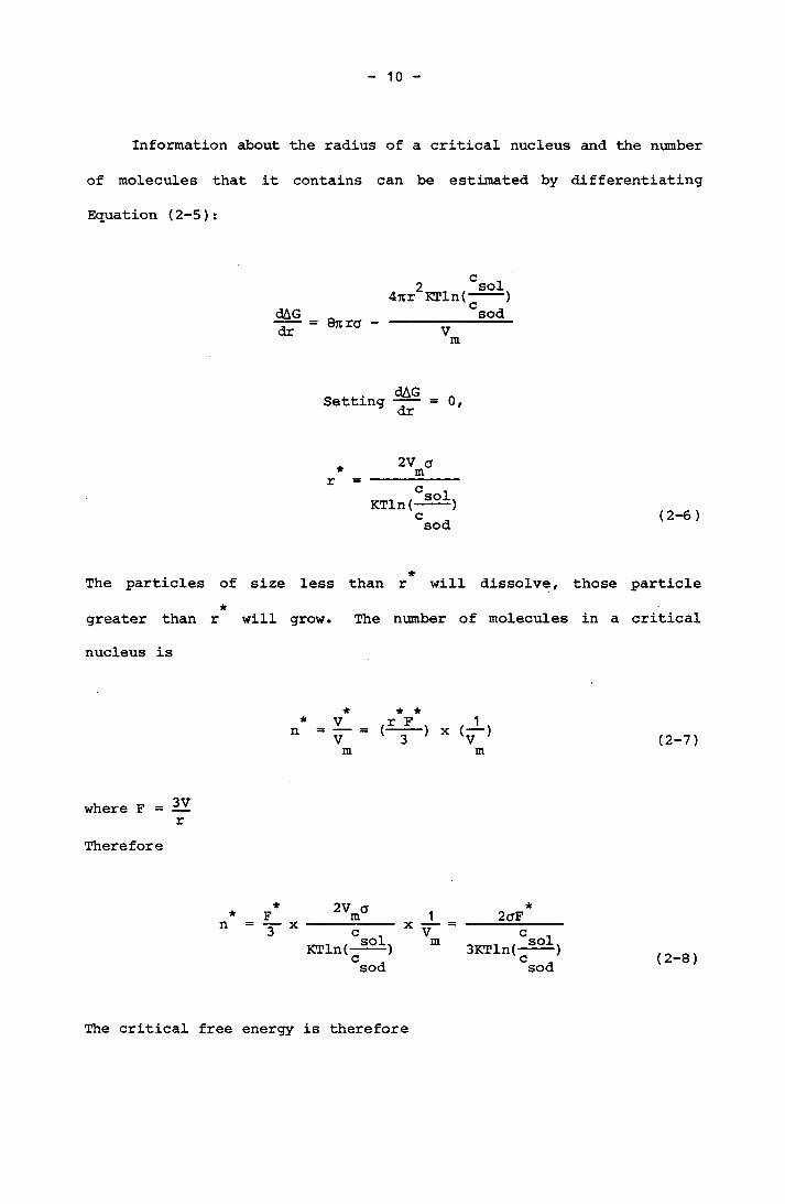
Information about the radius of a critical nucleus and the number
of molecules that it contains can be estimated by differentiating
Equation (2-5):
dAGdr Qrtra -
2 sol4ur KTln(---“)
CsodVm
Setting dAGdr 0,
*r2V a _____m
KTln(~~~)Csod (2-6)
*The particles of size less than r will dissolve, those particle*greater than r will grow. The number of molecules in a critical
nucleus is
*n★ *r F 1(—> X (-,
m (2-7)
where F = — rTherefore
F_3
2v am 2aFKTln(—^——) 3KTln(-^)
sod sod (2-8)
The critical free energy is therefore

11
c* * sol *AG = - n KTln(---- ) + aFCsod
*2qF3
*+ aF aF3 (2-9)
with the aid of Equation (2-8)
★F2 2 a V in
[(KTln(-^)]2Csod (2-10)
Iwhere (3 is a geometric shape factor
(2-11)
V[(3 = 16.76 (spheres), 2.22 (icosahedron), 22.30 (dodecahedron), 27.71
(octahedron), 32 (cube), 55.43 (tetrahedron)].Therefore the number of molecules in a critical nucleus will be in the
form
*n3 2 a Vmsol 3[KTln(---- )]
Csod (2-12)
The first equation for the rate of nucleation was described by Volmer
and Weber (1922;1929) and subsequent work was by Becker and Doring
(1935), also Nielsen (1964) and Kahlweit (1960). The rate of nuclea
tion (number of nuclei formed, cm ^s S is estimated by calculating
the rate at which the nucleus attains its critical size; ie.
12
J = A^exp[-AG /KT] = A^exp[-„ ' 3 2- p ° vm
(KT^lnf-^)2sod (2-13)
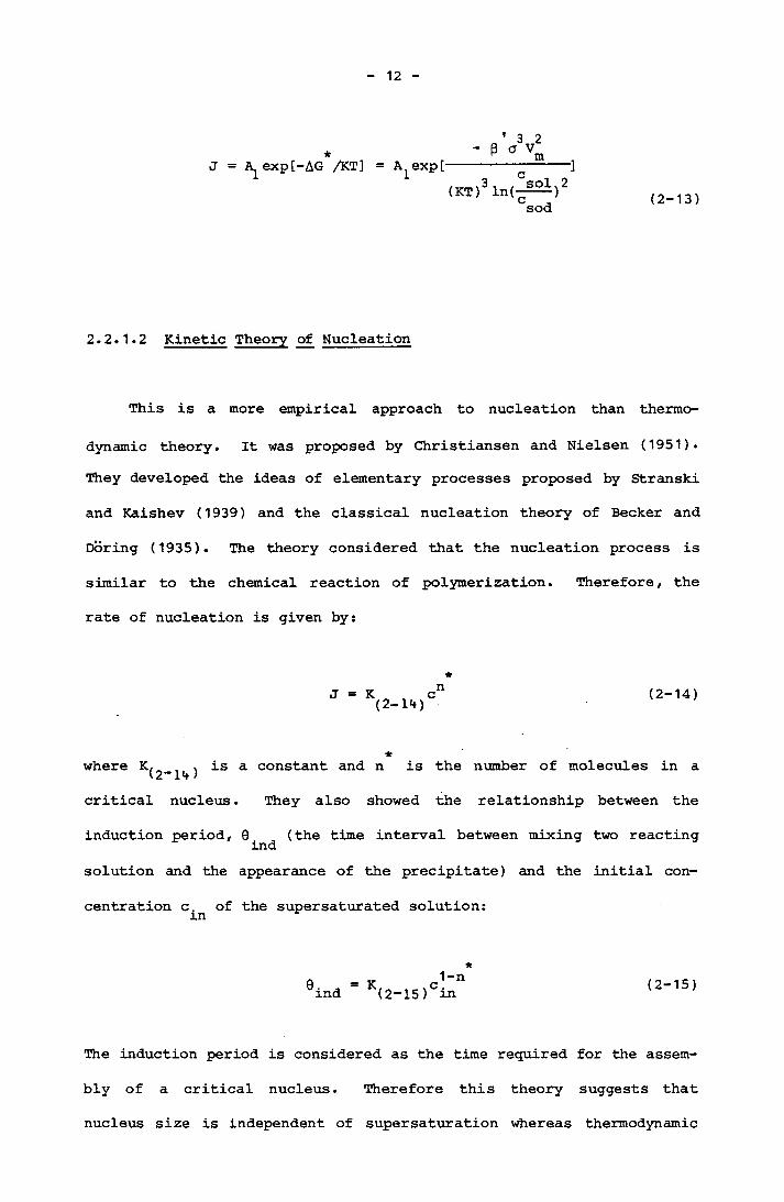
2.2.1.2 Kinetic Theory of Nucleation
This is a more empirical approach to nucleation than thermo
dynamic theory. It was proposed by Christiansen and Nielsen (1951). They developed the ideas of elementary processes proposed by Stranski
and Kaishev (1939) and the classical nucleation theory of Becker and
Doring (1935). The theory considered that the nucleation process is
similar to the chemical reaction of polymerization. Therefore, the
rate of nucleation is given by:
★J = K cn (2-14)(2-14)
*where K^-^) as a constant and n is the number of molecules in a
critical nucleus. They also showed the relationship between the
induction period, 9 (the time interval between mixing two reactingindsolution and the appearance of the precipitate) and the initial con
centration c of the supersaturated solution:
9.xnd K(2-15)*
c 1-nin (2-15)
The induction period is considered as the time required for the assem
bly of a critical nucleus. Therefore this theory suggests that
nucleus size is independent of supersaturation whereas thermodynamic

13
(classical) theory indicates a supersaturation-dependent nucleus size.
2.2.2 Heterogeneous Nucleation
Homogeneous nucleation only takes place when the solution is
dust-free. This is virtually impossible to achieve in practice.6 8Water that is prepared in the laboratory usualy contan 10 - 10 per
3cm of dust particles and under careful filtration, the number can be3 3reduced to less than 10 per cm . Nucleation from solution therefore
takes place in the presence of dust particles. From the theory of
homogeneous nucleation the. rate of nucleation is governed by the
overall free energy change associated with the formation of the criti
cal nucleus. It has been noticed that many reported cases of spon
taneous nucleation on further examination were found to be induced in
some way (Melia, 1965). Since heterogeneous nucleation takes place at
lower critical. supersaturation than homogeneous nucleation, the
overall free energy change is less than for homogeneous nucleation,
ie.
AG*' = <j)AG* (2-16)
* iwhere AG is the critical free energy change associated with
heterogeneous nucleation.
<j> is a factor that is less than unity
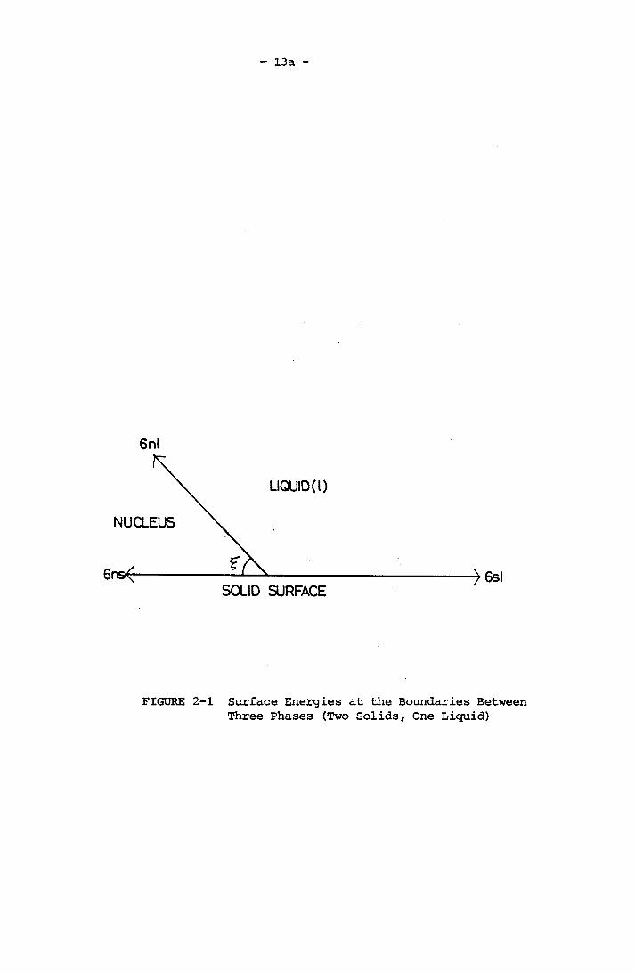
Figure (2-1) shows the balance of interfacial energies between solu
tion, nucleus and dust particles.
13a
6nl
LIQUID (l)
NUCLEUS
SOLID SURFACE
FIGURE 2-1 Surface Energies at the Boundaries Between Three Phases (Two Solids, One Liquid)
14
a , ,a and a are the interfacial energies of nucleus-liquid, nl si nssolid-liquid and nucleus-solid respectively. £ is the contact angle.
For 180° > £ > 0°
a , = a , + a , cos£ nl nl nl
Volmer (1945) derived the factor <{>, where
(2 +cos£)(1 - cos£)
(2-17)
(2-18)
if £ = 180°, this is the case of complete non-wetting,
l = 1, AG*' = AG*
This implies homogeneous nucleation.
If £ lies between 0° and 180°,<{) < 1; therefore
* • *AG < AG
This is the case of heterogeneous nucleation.
If £ = 0, which implies complete wetting of the solid-liquid system.
Therefore <£ =0, nucleation takes place on the solid which in this
case is a tiny crystal seed of the solution.
Turnbull and Vonnegut (1952) considered the catalytic potency of
the solid particles to nucleation in the solution based on crystallo
graphic theory. The basic postulate of this theory is that the inter
facial energy between nucleus and the catalytic surface element is a
minimum when the nucleus forms coherently. When the nucleus does not
15
match the solid particle, strain is induced in the crystal nucleus.
In general the nucleus will not match the solid particles perfectly
but are strained by an amount E,
E = (x - d0)/cL0 (2-19)
where x and d^ , are the lattice parameters of the nucleus in the
strained and strain-free condition respectively.
IThe lattice mismatch, 6 (disregistry), between the two solids is
defined as
6' = Ad/d0 (2-20)
where Ad is the difference in lattice parameter between solid and
nucleus.
If 6 > E/ the interface is said to be coherent. If 5 > E > 0,
the nucleus is said to be incoherent with the catalytic solid. In
general, the nuclei form coherently with the catalyst when the disre
gistry (6) ~ 0.005 - 0.015. The boundary condition for epitaxis or
oriented overgrowth is ~ 0.20. Nevertheless, Johnson (1951) had found
oriented overgrowth for 5 as large as 0.50.
2.2.3 Secondary Nucleation
Secondary nucleation is nucleation induced by crystals. It is a
special case of heterogeneous nucleation where the nucleation sites
are the crystal themselves. The fact that the supersaturated solution
16
nucleates much faster under crystal seeded condition is well known
(Mullin, 1972). This is sometimes called self-nucleation. Mason and
Strickland-Constable (1966) conducted extensive studies on secondary
nucleation and identified three types of crystal nucleation mechanisms .
1. Initial breeding - this was seeding due to microscopic particles.
They were attached onto dry seed-crystals and then swept off to
become new seeding sites.
2. Needle breeding - this was observed under very high supersatura
tions. The dentritic growth from the face of crystals broke off
and formed new nuclei.
3. Collision breeding - new nuclei were generated due to collision
of crystals with one another and also with the other solid parts
such as impeller and surface of the crystallization vessel.
Strictly speaking, the first two mechanisms cannot be classified as
secondary nucleation. The third mechanism is often considered as the
major source of secondary nuclei. Lai et. al. (1969) were among the
first to demonstrate conclusively the existence of collision breeding.
They carried out studies on MgSO^.TH^O, KC1 and KBr crystals. The
following conclusions were drawn:
1. Fluid shear alone did not give rise to nucleation.
2. High rates of nucleation resulted when a crystal maintained con
tact with a surface while moving about in a stirred solution.
3. Nucleation occurred when a crystal touched a solid object.
4. The rate of nucleation was strongly dependent on the supersatur-
tion.
17
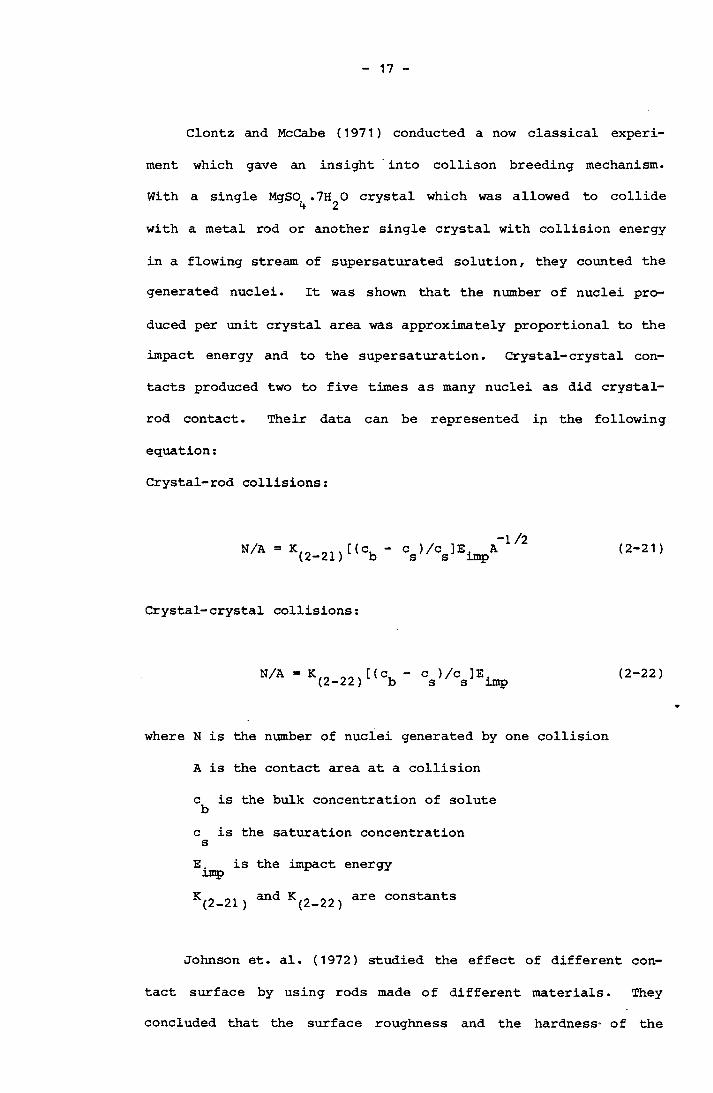
Clontz and McCabe (1971) conducted a now classical experi
ment which gave an insight into collison breeding mechanism.
With a single MgSO^.71^0 crystal which was allowed to collide
with a metal rod or another single crystal with collision energy
in a flowing stream of supersaturated solution, they counted the
generated nuclei. It was shown that the number of nuclei pro
duced per unit crystal area was approximately proportional to the impact energy and to the supersaturation. Crystal-crystal con
tacts produced two to five times as many nuclei as did crystal-
rod contact. Their data can be represented ip the following
equation:
Crystal-rod collisions:
N/A = K.0 , [(c, - c )/c ]E. A(2-21) b s s imp-1 /2 (2-21)
Crystal-crystal collisions:
N/A K(2-22)[(Cb c )/c ]E. s s imp (2-22)
where N is the number of nuclei generated by one collision
A is the contact area at a collision
c is the bulk concentration of solute bc is the saturation concentration sE, is the impact energy impK(2 21) and K(2 22) are constants
Johnson et. al. (1972) studied the effect of different con
tact surface by using rods made of different materials. They
concluded that the surface roughness and the hardness of the
18
crystal as well as the rod affected collision breeding. Only materials as hard as or harder than the crystal surface were capable of causng contact nucleation. Secondary nucleation was
referred to as "micro-attrition".
Cise and Randolph (1972a, 1972b) studied the effect of
secondary nucleation of potassium sulphate crystals in a seeded backmixed magma (MSMPR) crystallizer. The nuclei were conducted
in the 1.3 - 26 micron size range by a multi-channel coulterautomatic particle counter. Nucleation increased with supersa
turation, seed crystal mass and with the size and stirring rate. Nucleation also depended on crystal habit. They observed that
under the same size and mass concentration condition, polycrystalline habit generated more secondary nuclei than the microcrystalline habit crystals. This indicated that secondary nucleation occurred on a favoured face. In addition, at a given mass concentration, larger crystals were noticed to be more effective than smaller crystals in generating secondary nuclei.
The '’growth rates of crystals were size dependent, and decrease with decreasing size.
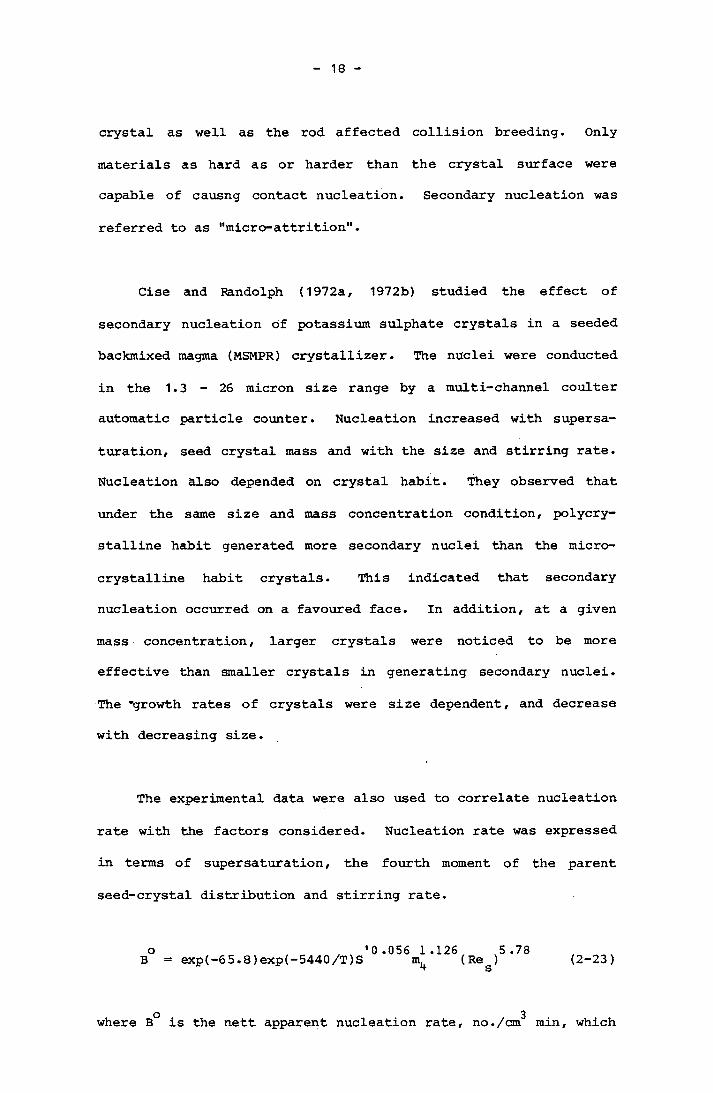
The experimental data were also used to correlate nucleation
rate with the factors considered. Nucleation rate was expressed
in terms of supersaturation, the fourth moment of the parent seed-crystal distribution and stirring rate.
o ' 0 .056 1 .126 5 .78B = exp(-65.8)exp(-5440/T)S m^ (Re^) (2-23)
where B° is the nett apparent nucleation rate, no./cm^ min, which
19
was obtained by extrapolating the measured CSD of macro
sized crystals back to zero sizeI
S is the solute supersaturation, g/L
m^ is the 4th moment about zero of population distribution
T is the absolute temperature, °K
Re is the Reynolds number for stirring s
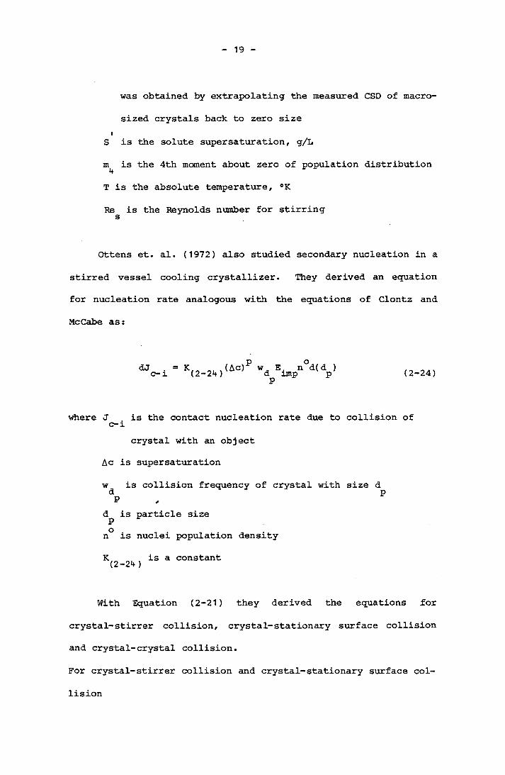
Ottens et. al. (1972) also studied secondary nucleation in a
stirred vessel cooling crystallizer. They derived an equation
for nucleation rate analogous with the equations of Clontz and
McCabe as:
r ■ = oi n(Ac)P w E. n°d(d )c-i (2-24) d imp pP (2-24)
where J is the contact nucleation rate due to collision ofc-i
Ac
wd
crystal with an object is supersaturation
is collision frequency of crystal with sizeP
d is particle size Pn° is nuclei population density
K is a constant(2-24 )
dP
With Equation (2-21) they derived the equations for
crystal-stirrer collision, crystal-stationary surface collision
and crystal-crystal collision.
For crystal-stirrer collision and crystal-stationary surface col
lision

20
J c-ms K(2-25) (Ac)PeMx (2-25)
where K p are constants
e is dissipated energy per unit mass of slurry by the
stirrer
M is total crystal mass above size, dX x
For crystal-crystal collision
J = K,„ . (Ac)PeM2 (2-26)c-c (2-26) x
In the experiments it was concluded that the nucleation rate is
determined by nucleation due to crystal-stirrer collisions.
Youngquist and Randolph (1972) studied the Ammonium-
Sulphate-Water system by using an MSMPR crystallizer, and corre
lated the experimental data of nucleation by the equation:
B° = 1.04x10"l8(rev./min.)7‘84Gl*22(MT)°’98 (2-27)
where B° is nucleation rate in no./cm minG is the crystal growth rate in microns/min
, 3is the solids concentration in g/cm
The experiment was tested at low supersaturation and it was
concluded that the nuclei were formed by micro-attrition of seed
crystals 1.26 to 25.4 microns in size. Nucleation rate was3determined from the birth distribution function B(L) as no./cm
micron. B(L) was calculated from population density data gen
erated from Coulter counter data with the growth term suppressed

21
in the population balance linear dependence on solids concentra
tion. This implies that secondary nuclei are generated by colli
sions of the seed crystals with the impeller blades. The growth
rate of the nuclei was very small compared to that of large cry
stals .
Bauer, Larson and Dallons (1974) also studied contact
nucleation of MgS0^.7H^0 in a continuous MSMPR crystallizer.
They mounted a MgS01+.7H20 crystal in a specialy designed crystal
contactor and immersed the crystal and contactor into the crys
tallizer.
The concentration of the nuclei in the solution was measured
with a Coulter counter. The number of nuclei generated due to
the controlled energy and frequency of contact between a perspex
rod and the mounted parent crystal were calculated from crystal
size data (CSD). This was related back to super saturation,
residence time, contact energy and frequency of contact. The
number of nuclei produced was found to increase with supersatura
tion. The nuclei production also increased with contact energy,
but decreased at energy inputs in excess of 15,000 ergs. Lower
nuclei production per contact was observed as frequency of the
contact increased. It was noticed that size-dependent growth
occurred as the number of nuclei increased with residence time
and indicated that the small crystals grew much slower than the
large crystals.
22
Sung et. al. (1973) demonstrated the effect of shear force
of a flowing stream in creating nuclei. They found that nuclei
were created from the parent crystal growing in a slightly
saturated solution by high fluid shear rates across the surface
of the crystal. The shear created nuclei were believed to be of
the size of the critical nucleus. This experiment is interesting
because it suggests the presence of the adsorption layer which is
in agreement with the crystal growth theory.
Randolph and Sikdar (1976) investigated the formation of
secondary nuclei of potassium sulphate in a MSMPR crystallizer.
They investigated the observation by Randolph and Cise (1972) and
Youngquist and Randolph (1972) of the very large population of
small-sized crystals in a MSMPR. This portion of population
disappeared in long-retention MSMPR experiments. In order to
explain this phenomeon, they conducted experiments on:
1. Short residence time MSMPR.
2. Long residence time MSMPR.
3. Seed trap experiments to test the hypothesis that nuclei
near 1 |im in size reattached on the parent macrocrystals, and
4. Ripener experiments by withdrawing a measured volume of
nuclei-laden crystallizer effluent and allowing it to ripen
for a period of time.
They concluded that only a fraction of originally formed secon
dary nuclei survived to populate the large size ranges. The
fraction of surviving nuclei increased with supersaturation,
23
therefore the correlated nucleation kinetics was based on observ
able, not viable nuclei.
Garside and Larson (1978) observed secondary nucleation for
potash alum and magnesium sulphate heptahydrate directly by
microscope examination. A crystal, approximately 3 mm in size,
was glued onto a support rod in the saturated solution contained
in a cell. The temperature of the solution was controlled by
thermostatically-controlled criculating water outside the cell.
The contact nucleation was achieved by rotating a contacting rod.
Photomicrographs were taken to record the crystals and nuclei
generated. The data indicated:
1. Secondary nuclei were readily produced as a result of attri
tion of a crystal surface by a solid object, even at very
low contact energies.
2. The nuclei were formed in both supersaturated and unsa
turated solutions. But the nuclei dissolved rapidly in
unsaturated solution.
3. Secondary nuclei produced in supersaturated solution were
over the size range 1 to 50 ^m. The number of large
'nuclei' was found to relate to the level of supersatura-
tion.
4. Many of the nuclei smaller than about 10 |im seemed to grow
very slowly or did not grow at all.
In a recent paper given by Larson (1982), he made a very
interesting suggestion on the mechanism of secondary nucleation.
Studies of sliding contact on the crystal produced more crystals
24
and nearly all appeared to have the characteristic habit immedi
ately (Garside and Larson, 1979; Rusli et. al., 1980; Berglund
et. al., 1981), even sliding contact had less energy than direct
contact. This piece of information strongly suggests the
existence of a semi-order partially desolvated layer near the
surface of the growing crystal, which is the starting point for
many crystal growth theories and must be the prime source of
secondary nuclei.
In Larson's paper, he also listed the findings of secondary
nucleation works by all investigators in the past decade:
1. It occurs as a strong function of supersaturation, more spe
cially, as a function of the rate of growth of the contacted
surface.
2. A variety of sizes are produced ranging from 2 ^,m to 40 p,m.
3. Number and size distribution are dependent on contact
energy, supersaturation , hardness of contactor. Sliding
contacts produce more nuclei.
4. Most particles immediately exhibit a characteristic habit.
5. Number is an inverse function of temperature.
6. Certain highly charged anions as well as certain dyes and
surface active agents inhibit nucleation.
7. Fluid shear causes nucleation.
Similarly for the growth of nuclei:
1. Very small nuclei tend not to grow unless the supersatura
tion is increased above that at which they were produced.
25
2. Intermediate size nuclei exhibit growth dispersion.3. Growth is a strong function of initial size.
4. Impurities change the growth dispersion characteristics.
2.3 CRYSTAL GROWTH FROM SOLUTION
Phase change from solution to solid takes place in the supersa
turated solution governed by the principles of thermodynamics. After
the formation of a stable nucleus, they continue to grow into cry
stals. Crystal growth rate is dependent on supersaturation, but other
factors such as relative velocity of crystal in the solution, crystal
size and impurities are able to affect the crystal growth. The degree
of dependence on these factors varies greatly between the molecular
compound being formed because of the different crystal growth mechan
ism. The theories of crystal growth are numerous, but there is still
no universal theory to explain crystal growth rate. All the theories
are only applicable to certain aspects of crystal growth. Crystal
growth is a complex process. The crystallization of ionic substances
from aqueous solution can involve the following processes (Mullin, 1972 ) :
1 . Bulk diffusion of solvated ions through the diffusion boundary
layer.
2. Bulk diffusion of solvated ions through the adsorption layer.
3. Surface diffusion of solvated or unsolvated ions.
4. Partial or total desolvation of ions.
5. Integration of ions into the lattice.
6. Counter-diffusion of released water through the adsorption layer.
7. Counter-diffusion of water through the boundary layer.

26
Theories of crystal growth can be broadly classified under sur
face energy theories, surface processes theories and diffusion
theories. Surface energy theories have failed to gain general accep
tance. The rest of the theories are still very popular and continue
to improve and expand in order to explain the experimental crystal
growth data.
2.3.1 Surface Energy Theories
In an isolated drop of liquid there is minimum free energy and
area. Gibbs (1928) suggested that the growth of crystal could be
treated as a special case of this principle. This means that the
total free energy of a crystal in equilibrium with its surroundings at
constant temperature and pressure would be a minimum for a given
volume. Accordingly, the shape of such a crystal would be
n£A,G, = minimum. i i (2-28)
where A is the area of the ith face of a crystal bounded by n faces,
is the surface free energy per unit area of the ith face.
In other words, the crystal would grow in such a manner to main
tain a minimum surface free energy for a given volume developed into an 'equilibrium' shape.
This simple concept of crystal growth was developed by Wulff
(1901). Mathematical proof was given by Hilton (1903), Liebman
(1914), Von Lane (1943), Strickland-Constable (1968). However, the

27
analogy of liquid droplet for crystal is an over simplification. In a
liquid atoms and molecules are randomly dispersed whereas crystal
molecules have to incorporate into a crystal lattice structure. The
presence of impurities, solvent molecules and solution flow condition
always change the growth rate of the individual crystal face. In gen
eral this theory fails to explain the effects of supersaturation and
solution movement on the crystal growth rate. As a result, it is not
generally accepted.
2.3.2 Surface Processes Theories
2.3.2.1 Introduction - Surface Structure
The majority of the crystal growth theories have been derived
from fundamental studies of the surface structure of crystals by Kos-
sel (1934) and Stranski (1928, 1930, 1939). According to these dis
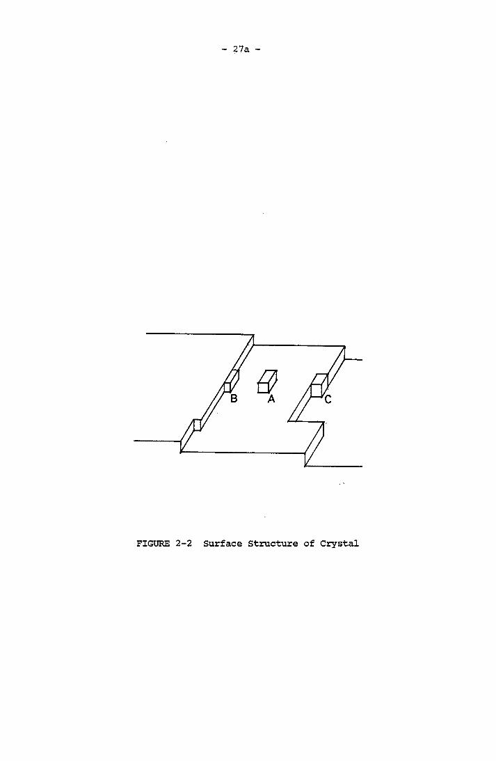
cussions, there are various energetically favorable sites for the attachment of solute molecules or growth units. (Figure (2-2)).
The flat area of a crystal face is energetically unfavourable for
molecule incorporation onto the crystal. This is position A in Figure
(2-2). Position B is more energetically favourable where the molecule
is attached and bonded onto the step face as well as to the surface.
The most energetically favourable location is indicated by C, where
three sides of the molecular cube are bonded. It is said to be kink-
bonded because the molecule is bonded in a kink of a step. Growth
molecules diffuse from the bulk of the solution onto the crystal sur
face and incorporate into kinks. The kinks move along the step and
eventually cover the face. Based on Kossel-Stranski's view of surface
27a
FIGURE 2-2 Surface Structure of Crystal
28
structure, Volmer (1939) used the Becker-Doring theory (1935) of
nucleation to describe the growth of crystals by a surface-nucleation
mechanism. This established the basis of surface processes for subse
quent growth theories. The growth molecules arrive at the surface of
the crystal, and migrate freely over the surface (surface diffusion).
The molecules eventually incorporate into crystal lattice or desorb
along the migration. Therefore, there will be a loosely adsorbed
layer of growth molecules at the crystal interface.
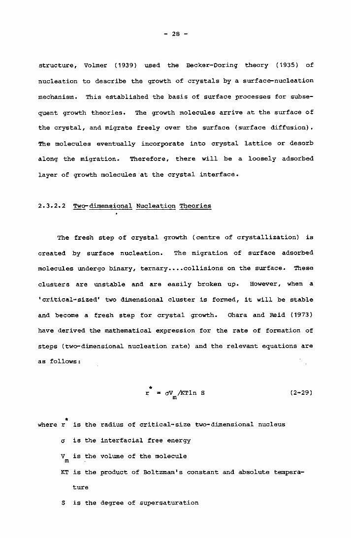
2.3.2.2 Two-dimensional Nucleation Theories
The fresh step of crystal growth (centre of crystallization) is
created by surface nucleation. The migration of surface adsorbed
molecules undergo binary, ternary....collisions on the surface. These
clusters are unstable and are easily broken up. However, when a
'critical-sized' two dimensional cluster is formed, it will be stable
and become a fresh step for crystal growth. Ohara and Reid (1973)
have derived the mathematical expression for the rate of formation of
steps (two-dimensional nucleation rate) and the relevant equations are
as follows:
★r = qV /KTln S (2-29)m
★where r is the radius of critical-size two-dimensional nucleus
a is the interfacial free energy
V is the volume of the molecule mKT is the product of Boltzman's constant and absolute tempera
ture
S is the degree of supersaturation
29
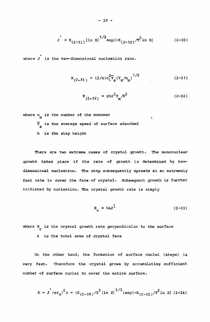
(2-30)
where J is the two-dimensional nucleation rate
K (2-31)
K (2-32)
where n is the number of the monomerm •
v is the average speed of surface adsorbed sh is the step height
There are two extreme cases of crystal growth. The mononuclear
growth takes place if the rate of growth is determined by two-
dimensional nucleation. The step subsequently spreads at an extremely
fast rate to cover the face of crystal. Subsequent growth is further
initiated by nucleation. The crystal growth rate is simply
where R is the crystal growth rate perpendicular to the surface cA is the total area of crystal face
On the other hand, the formation of surface nuclei (steps) is
very fast. Therefore the crystal grows by accumulating sufficient
number of surface nuclei to cover the entire surface.
R = hAJ (2-33)c

30
K(2-35) “ 2vs(anmA)2hl/2vm/2 (2‘35>
Obviously there are intermediate rate models between these two
extremes such as Nielsen's (1964) birth and spread model.
2.3.2.3 Screw Dislocation Theory of BCF
The two-dimensional nucleation theories predict the requirement
of sufficient supersaturation in order for surface nucleation to take place. However, many crystal faces in solutions of relatively low
supersaturation can grow at a rate much faster then surface nucleation
mechanism can explain. Therefore it seems that the surface nucleation
mechanism and Kossel's model are not a correct explanation of the cry
stal growth rate. Frank (1949) postulated that the role of crystal
dislocations in crystal growth is important. These dislocations espe
cially screw dislocations provide crystal growth sites. The step is
produced on the face at a height equal to the Burger's vector. This
step is perpetuated on the face 'up a spiral staircase' as the crystal
grows by adsorption of molecules. Since t£e step is self-
perpetuating, it by-passes the requirement of surface nucleation and
provides an explanation for the crystal growth rate at relatively low
supersaturation.
Subsequently Burton, Cabrera and Frank (1951) developed the well
known BCF crystal growth kinetics based on Frank's spiral growth con
cept. In this model, if the surface is considered to contain multiple
straight steps or islands, molecules are adsorbed onto the surface and
then diffuse along the surface toward energetically favourable kink
sites. Some molecules proceed directly toward the kinks, others
impinge onto the step and diffuse along the step toward kinks (ledge

31
or edge diffusion) . The velocity of a straight step in a group of
parallel straight steps equally spaced by a dimension Y is:o
Vv = (V /hX ) (2D C Bay )tanh(Y /2X ) (2-36)0° m x s SE r 0 os
where X is the mean diffusion distance on the surface in time sD is the surface diffusion coefficient, sC is the equilibrium concentration of surface adsorbed SEmolecules at the given temperature
6 is the rate of removal of molecules from a molecular rcluster
a' = S-1 where S is the degree of supersaturation
y is the kink retardation factor oIf screw dislocations exist on the surface/ the growth rate perpendic
ular to the surface is calculated by the apparent angular velocity of
the spiral, go* The radius of curvature can be related to go and also
to the step spacing between spiral, Y . The final equations are:
R = vVYo = K(2-38 )Ta' 2tanh(K(2_3g } /To' ) (2-37)
(2-38 )2D C KB y s SE ^r’o
19X a s (2-38)
where a is the interfacial energy between crystal and solution,
= 19aV /2KX(2-39) m s (2-39)
If a is very low, tanh ( K ^ )/Ta) ~ 1
32
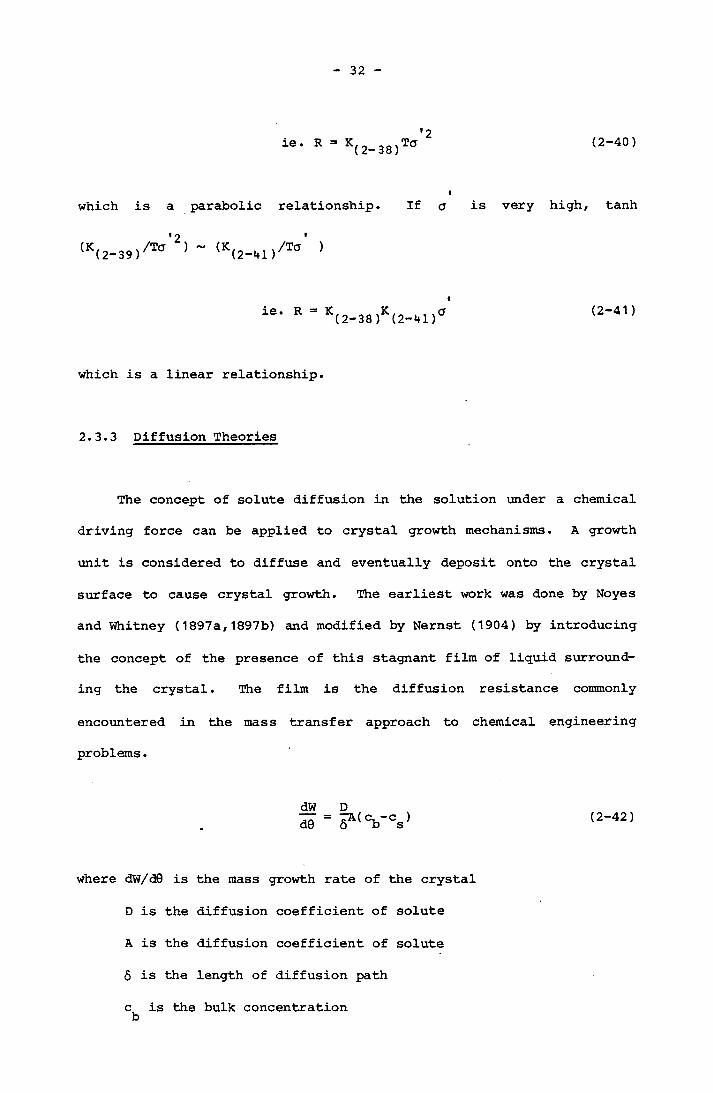
iS* R = K(2-38)TCJ'2 (2-40)
which is a parabolic relationship. If a is very high, tanh
(K(2-39)/TCT’2> ~ <K(2-41)/TO’ 1
1S* R K(2-38)K(2-41)a (2-41)
which is a linear relationship.
2.3.3 Diffusion Theories
The concept of solute diffusion in the solution under a chemical
driving force can be applied to crystal growth mechanisms. A growth
unit is considered to diffuse and eventually deposit onto the crystal
surface to cause crystal growth. The earliest work was done by Noyes
and Whitney (1897a,1897b) and modified by Nernst (1904) by introducing
the concept of the presence of this stagnant film of liquid surround
ing the crystal. The film is the diffusion resistance commonly
encountered in the mass transfer approach to chemical engineering
problems.
dW D(2-42)
where dW/d0 is the mass growth rate of the crystal
D is the diffusion coefficient of solute
A is the diffusion coefficient of solute
6 is the length of diffusion path
c is the bulk concentration b
33
c is the equilibrium concentration
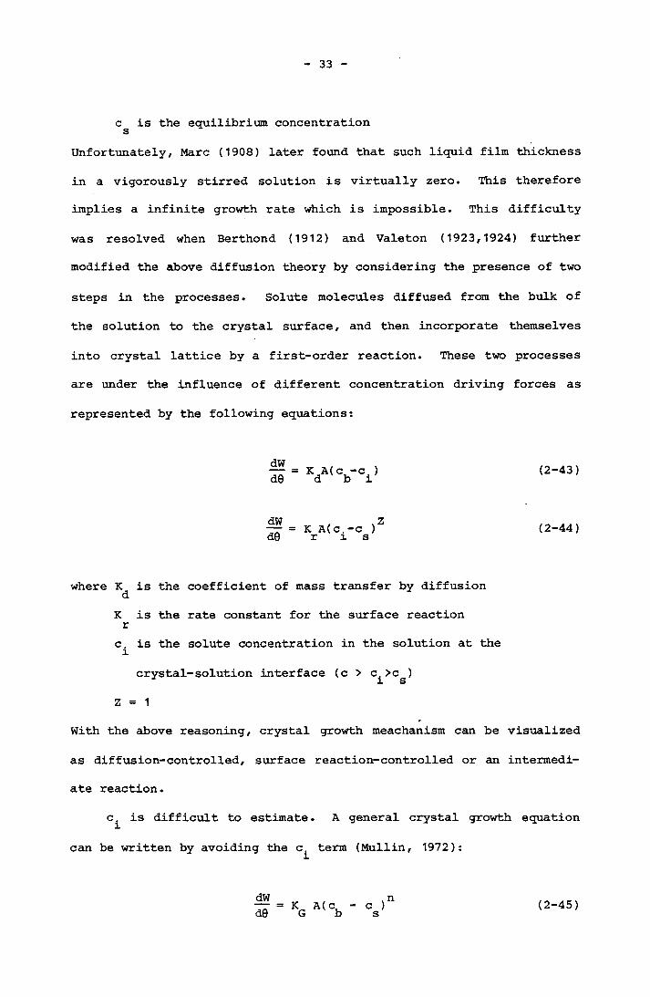
Unfortunately, Marc (1908) later found that such liquid film thickness
in a vigorously stirred solution is virtually zero. This therefore
implies a infinite growth rate which is impossible. This difficulty
was resolved when Berthond (1912) and Valeton (1923,1924) further
modified the above diffusion theory by considering the presence of two
steps in the processes. Solute molecules diffused from the bulk of
the solution to the crystal surface, and then incorporate themselves
into crystal lattice by a first-order reaction. These two processes
are under the influence of different concentration driving forces as
represented by the following equations:
dWd0 K A(c -c d b (2-43)
dWd0
, . ZK A(c.-c ) r is (2-44)
where KdKrc.l
is the coefficient of mass transfer by diffusion
is the rate constant for the surface reaction
is the solute concentration in the solution at the
crystal-solution interface (c > c >c )
Z = 1
With the above reasoning, crystal growth meachanism can be visualized
as diffusion-controlled, surface reaction-controlled or an intermedi
ate reaction.
c^ is difficult to estimate. A general crystal growth equation
can be written by avoiding the c^ term (Mullin, 1972):
A( cb c ) sndW
d0 (2-45)

34
where is the overall crystal growth coefficient
n is the so called 'order' of overall crystal growth process
This empirical equation is commonly used in interpreting crystal
growth data.
Burton, Cabrera and Frank (1951) also carried out rigorous
mathematical calculation to derive the rate of crystal growth by
applying the concept of bulk diffusion to two-dimensional steps or
dislocation steps. The molecules diffuse directly to the kinks
without surface adsorption followed by surface diffusion and ledge
diffusion, the final equation contains the concentration boundary
layer thickness. Certain assumption used in the calculation were cri
ticised by Ohara and Reid (1973). Chernov (1961) simplified BCF bulk
diffusion model by assuming a step as a line sink, ie. neglecting
kinks. Therefore the diffusion fields considered were only created by
the bulk concentration and steps. Again the final crystal growth
equation contains the concentration boundary layer thickness. These
two theoretical approches deal with diffusion controlled growth
mechanism. Other theoretical treatments were also published in the
literature (Frisch and Collins, 1952,1953; Ham, 1958; Goldstein, 1968;
Cable and Evans, 1967). For many sparingly soluble salts the con
trolled mechanism is not diffusion controlled because growth rate does
not increase with stirring. Referring to the previous equations sug*-
gested by Berthond and Valeton, the first order surface reaction is
questionable because this will render n in Equation (2-45) to be
unity. In fact many inorganic salts growth data published in the
literature require n=1.5 to 2 to fit Equation (2-45). Therefore, a
more realistic model for surface reaction will have Z > 1. This also
suggests the existence of intermediate rate controlled mechanisms

35
between the diffusion and surface reaction. A quantitative measure of the degree of diffusion or surface reaction control was proposed by Garside (1971) through the concept of effectiveness factors.
ri = (measured over-all growth rate) / (growth rate expected when the rcrystal surface is exposed to conditions in the bulk solution)
K (c - c ) r b s (2-46)
When n 1/ the surface reaction mechanism is increasingly dominant
2.3.4 Further Development of Surface Processes Theories
2.3.4.1 Introduction
Most sparingly soluble inorganic salts grow by surface reaction (processes) controlled mechanisms. The growth rate is controlled by the molecules or ions incorporate into the crystal lattice through
dehydration and migration to the kinks. The following theories are a further development of surface processes theories mentioned in Section
(2.3.2) concentrating on the role of growth unit incorporation into crystal lattice as the rate controlling step for crystal growth from
solutions.
2.3.4.2 Surface Reaction Models of Doremus (1958,1970)
Two models were proposed, based on the following mechanisms:
36
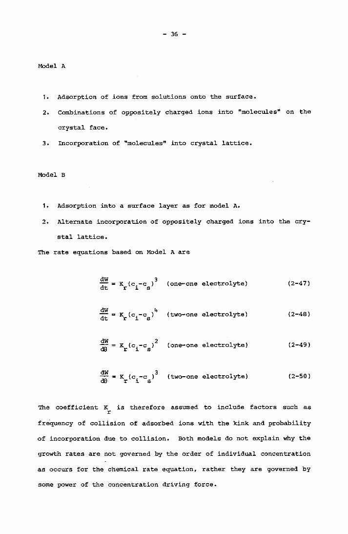
Model A
1. Adsorption of ions from solutions onto the surface.
2. Combinations of oppositely charged ions into "molecules" on the
crystal face.
3. Incorporation of "molecules" into crystal lattice.
Model B
1. Adsorption into a surface layer as for model A.
2. Alternate incorporation of oppositely charged ions into the cry
stal lattice.
The rate equations based on Model A are
dWdt
dWdt
K (c.-c ) r i s
K (c.-c ) r i s
(one-one electrolyte)
(two-one electrolyte)
(2-47)
(2-48)
dW 2— = K (c.-c ) (one-one electrolyte) d0 r i s (2-49)
— = K (c.-c )3 (two-one electrolyte) (2-50)d9 r i s
The coefficient K is therefore assumed to include factors such as rfrequency of collision of adsorbed ions with the kink and probability
of incorporation due to collision. Both models do not explain why the
growth rates are not governed by the order of individual concentration
as occurs for the chemical rate equation, rather they are governed by
some power of the concentration driving force.
37
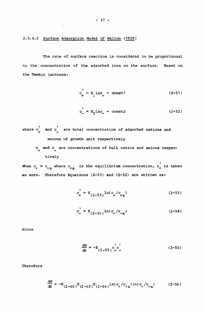
2.3.4.3 Surface Adsorption Model of Walton (1920)
The rate of surface reaction is considered to be proportional
to the concentration of the adsorbed ions on the surface. Based on
the Temkin isotherm:
c = K Inc + constl (2-51)+ 1 +
c_ = I^lnc^ + const 2 (2-52)
I fwhere c and c are total concentration of adsorbed cations and +anions of growth unit respectively
c^ and c are concentrations of bulk cation and anions respec
tivelyI
When c = c where c is the equilibrium concentration, c, is taken + +s + s +as zero. Therefore Equations (2-51) and (2-52) are written as:
°i = K(2-53,ln(C+/C+s) (2'53)
■0 " K(2-54)ln(c-/c-s) <2'54>
Since
dWd0
I tK o re (2-55) c c + - (2-55)
Therefore
dWd0 -K(2-55)K(2-53)K(2-54)ln<C+/C+s,ln(C-/C-s) (2-56)
38
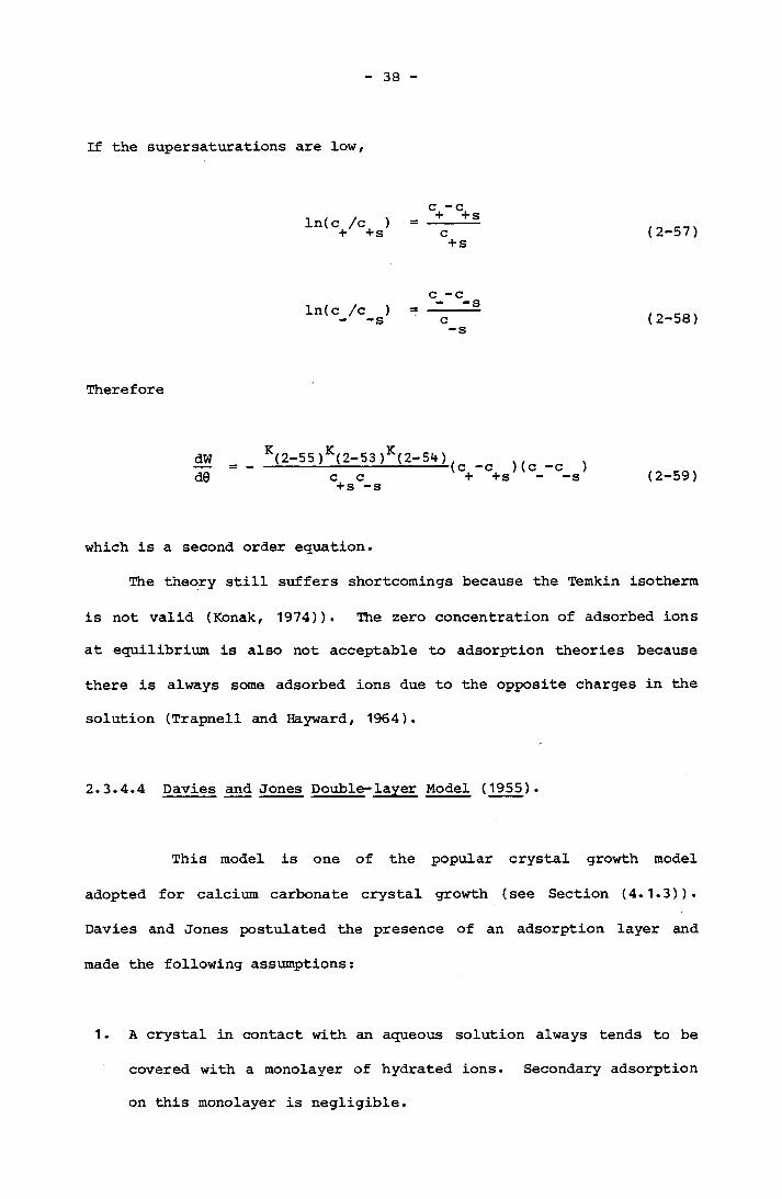
If the supersaturations are low,
ln(c /c ) + +s c+ s (2-57)
ln(c /c )- -s (2-58)
Therefore
dWd0
K(2-55)K(2-53)K(2-54) _ ,--------------------—(c -c )(c -c )c c + +s - -s+ s -s (2-59)
which is a second order equation.
The theory still suffers shortcomings because the Temkin isotherm
is not valid (Konak, 1974)). The zero concentration of adsorbed ions at equilibrium is also not acceptable to adsorption theories because
there is always some adsorbed ions due to the opposite charges in the
solution (Trapnell and Hayward, 1964).
2.3.4.4 Davies and Jones Double-layer Model (1955 ) .
This model is one of the popular crystal growth model
adopted for calcium carbonate crystal growth (see Section (4.1.3)).
Davies and Jones postulated the presence of an adsorption layer and
made the following assumptions:
1. A crystal in contact with an aqueous solution always tends to be
covered with a monolayer of hydrated ions. Secondary adsorption
on this monolayer is negligible.

39
2. Crystallization occurs through the simultaneous dehydration of
pairs of cations and anions.
3. Every ion striking the surface from a saturated solution enters
the mobile adsorbed monolayer.
A brief account of the derivation of the rate equation is given
in Section (4.1.3). The final equation is in the form
dc 1/2 2- ¥ = kdjn[(°+°-) - °s) <2'60)
where C is the solute concentration at any instant
K is the constant for the Davies and Jones model DJN is the number of particles per unit volume at any instant.
2.3.4.5 Surface Reaction Model of Konak (1971,1974)
Konak (1971) surveyed the crystal growth theories available and
extracted the important aspects of these theories to formulate a new model for surface reaction - controlled growth of crystals from solu
tion. He considered the crystallization process consisted of mass transfer followed by surface reaction, and then adsorption, dehydra
tion and counter diffusion. He explained that the growth rate was
proportional to (c-c ) instead of to the concentration of the solutesbecause the free energy of the adsorbed layer at equilibrium concen
tration of crystal is a minimum. In order to maintain such a minimum,
excess ions will have to be "rejected" by deposition on the crystal
surface. Adsorption layer concentration can be expressed as (De Boer,
1968)
40
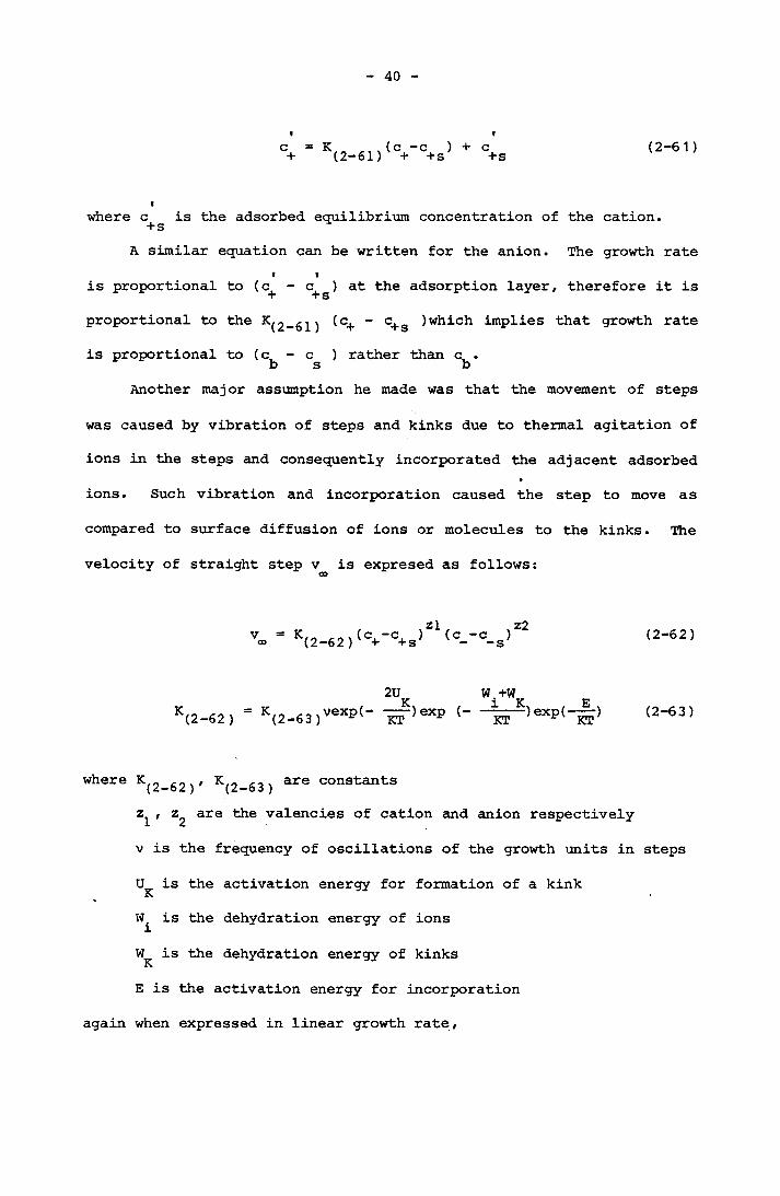
c+ K(2-61)(C+*C+s) + c + s (2-61)
where c+ is the adsorbed equilibrium concentration of the cation.
A similar equation can be written for the anion. The growth ratef Vis proportional to (c - c ) at the adsorption layer, therefore it is+ + s
proportional to the 2 — 61 ) ^c+ ” c+s implies that growth rateis proportional to (c - c ) rather than c .b s b
Another major assumption he made was that the movement of steps
was caused by vibration of steps and kinks due to thermal agitation of
ions in the steps and consequently incorporated the adjacent adsorbed
ions. Such vibration and incorporation caused the step to move as
compared to surface diffusion of ions or molecules to the kinks. The
velocity of straight step v is expresed as follows:
V» = K(2-62)<°+-C+S)Z1(0--C-s)Z2 (2-62)
2U W.+WK(2-62) = K(2-63)VeXp(- ^T)eXp (- (2-63)
where $2)' K(2 63) are constants, z^ are the valencies of cation and anion respectively
v is the frequency of oscillations of the growth units in steps
U is the activation energy for formation of a kink J\
W. is the dehydration energy of ions
W is the dehydration energy of kinks K.E is the activation energy for incorporation
again when expressed in linear growth rate

41
°° h , >zl, . z2--- = K —(c -c ) (c -c )Y 2-62 Y + +s - -s (2-64)
for equal ionic concentration in the bulk solutions,
R = K (c — c ) r b s (2-65)
where
z Z1 + Z2 (2-66)
and
Kr K(2“62)Y (2-67)0
2.3.4.6 Nielsen Electrolyte Crystal Growth Theory (Nielsen, 1982)
Recently Nielsen derived the theoretical explanation to
apply BCF surface spiral mechanism to conventional surface reaction,-
controlled growth rate equation. Many sparingly soluble inorganic
salts follow a parobolic rate law as indicated by the familiar equa
tion
dLd0 K (c,-c ) r b s (2-68)
where L is the size of the crystal
9 is the time
According to Nielsen, Equation (2-68) can also be written as

42
d0 = K(2-69)(S 1) (2-69)
where K is the rate constant(2-69)This is similar to the parabolic law obtained from the BCF screw
dislocation theory. A generalized version of Equation (2-68) for an
A B electrolyte is: a p
<£ = 1C (n1/e . ki/c.2d0 K(2-70)'U sp ' (2-70)
[Aa+]a [B^]Pwhere II
C = a + pK is the solubility product sp
Similarly Equation (2-70) can be written as:
dL 2d0 ~ K(2-69)(S 1} (2-71)
where S is defined as (II/K )sp1/C
K(2 69 ) WaS ^er^ved by Nielsen assuming that the rate-determining step was the integration of ions into kinks in growth spirals. The ions
entering from adsorption layer formed by ions in equivalent (elec
troneutral) ratio. The layer is in adsorption equilibrium with the
solution. The final result of K as a complex term which con-(2-69 )
tains step height/ interfacial energy, ion pair association constant.
adsorption equilibrium constant and is temperature dependent.
43
2.4 CONCLUSIONS FOR CHAPTER 2
Crystallization is still not fully understood because of the com
plexities involved in the process. However important progress had
been made in the past 20 years for both theoretical and experimental
treatment of the subject. The role of secondary nucleation in indus
trial crystallization processes is already well recognized. This
leads to new criteria in crystallizer design for crystal size distri
bution control. Factors such as the degree of supersaturation, hydro-
dynamic condition, impurities, power input, magma density are all
treated with improved theoretical bases on nucleation and crystal
growth. Recent works by Larson (1982) and Nielsen (1982) have brought
out the significance of crystal surface processes. Kossel's surface
concept in conjunction with BCF mechanism seems to be still the most
important approach. When it combines with the adsorption desolvated
ion layer concept it can offer a more accurate prediction for cry
stallization from solution. It is therefore important, as suggested
by Larson (1982) that detailed studies of the crystal-liquid interface
at the 100°A layer will provide useful information relavant to many
unanswered questions.
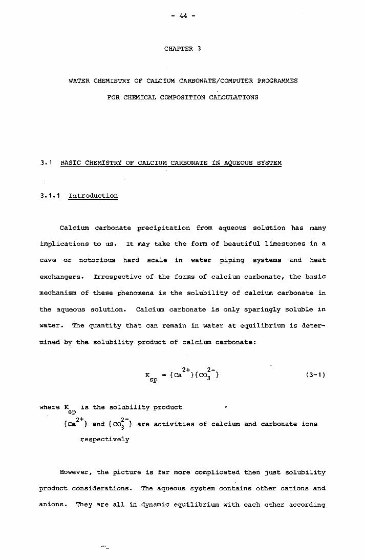
44
CHAPTER 3
WATER CHEMISTRY OF CALCIUM CARBONATE/COMPUTER PROGRAMMES
FOR CHEMICAL COMPOSITION CALCULATIONS
3.1 BASIC CHEMISTRY OF CALCIUM CARBONATE IN AQUEOUS SYSTEM
3.1.1 Introduction
Calcium carbonate precipitation from aqueous solution has many
implications to us. It may take the form of beautiful limestones in a
cave or notorious hard scale in water piping systems and heat
exchangers. Irrespective of the forms of calcium carbonate, the basic
mechanism of these phenomena is the solubility of calcium carbonate in
the aqueous solution. Calcium carbonate is only sparingly soluble in
water. The quantity that can remain in water at equilibrium is deter
mined by the solubility product of calcium carbonate:
2+ 2-K = {Ca }{C0~ } (3-1)Sp *
where K is the solubility product sp2+ 2“{Ca } and {CO^ } are activities of calcium and carbonate ions respectively
However, the picture is far more complicated then just solubility
product considerations. The aqueous system contains other cations and
anions. They are all in dynamic equilibrium with each other according

45
to the temperature, pressure and ionic strength of the system. The
carbonate ion, which is part of calcium carbonate solubility product ,
is further determined by the dynamic distribution of carbonic species
in the water. Carbonic species distribution is the single most impor
tant factor to determine how much calcium carbonate can remain in
water. There are two different systems for carbonic species distribu
tion, those for solutions in contact and not in contact with a gas
phase.
3.1.2 Carbonate Species Distribution in a Closed System (Stumm and
Morgan, 1970; Loewenthall and Marais, 1976)
When water is not in contact with a gaseous phase, the equilibria
of carbonic acid can be determined by the following equations:
C02 + H20 H2C03 (3-2)
h2co3 ~—H+ + hco3 (3-3)
- ___a. + 2“HC03 H + C03 (3-4)
+ —H20 7—^ H + OH (3-5)
The respective equilibrium constants are Equations (3-6), (3-7) and
(3-8) .
{H+}{HCcf}((cc>2}+{ h2co3> )
{H+ }{HC0"}-----------* = K1{h2co3} (3-6)
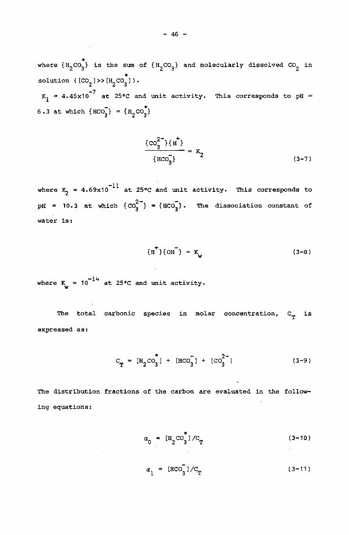
46
where {H2C03} is the sum of {^CO^} and molecularly dissolved CO in*
solution ( [C02]>> [H^CO^] ).-7= 4.45x10 at 25°C and unit activity. This corresponds to pH =
_ *6.3 at which {HC03> = {H2C03>
{C0*‘}{H+}------ :—-- k2{HC03> (3-7)
where = 4.69x10 11 at 25°C and unit activity. This corresponds to2- -pH = 10.3 at which {C03 } = {HC03}. The dissociation constant of
water is:
{H+}{OH~} = K (3-8)w
-14where K = 10 at 25°C and unit activity, w
The total carbonic species in molar concentration, CT is
expressed as:
CT* —
[h2co3] + [hco3] + [CO (3-9)
The distribution fractions of the carbon are evaluated in the follow
ing equations:
“o = (H2C031/CT (3-10)
a 1 [hco3)/cT (3-11)
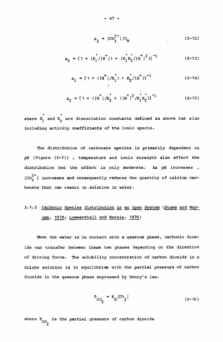
47
a2 = [CO^]/CT (3-12)
aQ = {1 + (K1'/[H+]) + (K^K^/t^]2)}"1 (3-13)
a1 = {1 + ([E+]/k[) + K2 / [ H+ ] } ”1 (3-14)
a2 = { 1 + ([h+]/k2 + ( [h+]2/klk2 )} 1 (3-15)
V Iwhere and are dissociation constants defined as above but also
including activity coefficients of the ionic specis.
The distribution of carbonate species is primarily dependent on
pH (Figure (3-1)) , temperature and ionic strength also affect the
distribution but the effect is only moderate. As pH increases , 2-[CO^ ] increases and consequently reduces the quantity of calcium car
bonate that can remain in solution in water.
3.1.3 Carbonic Species Distribution in an Open System (Stumm and Mor
gan , 1970 ; Loewenthall and Marais, 1976)
When the water is in contact with a gaseous phase, carbonic diox
ide can transfer between these two phases depending on the direction
of driving force. The solubility concentration of carbon dioxide in a
dilute solution is in equilibrium with the partial pressure of carbon
dioxide in the gaseous phase expressed by Henry's law.
K [CO ] H 2 (3-16)
where P is the partial pressure of carbon dioxide
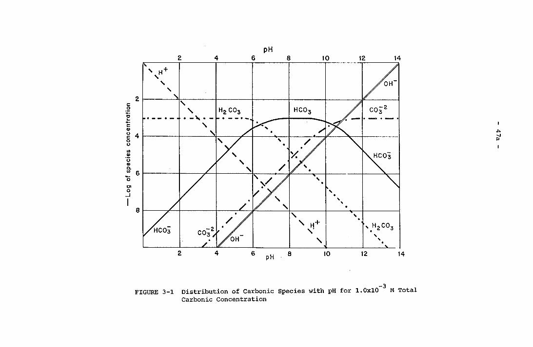
47a
O \
CVJ Tj-
U> CD
uojiDJjuaouoo sajoads jo Bo-) —
FIGURE 3-1 Distribution of Carbonic Species with pH for 1.0x10 M Total Carbonic Concentration

48
K is the Henry's constantH[CC^ ] is the concentration of dissolved CO^
Because of this additional equilibrium equation, carbon dioxide
transfer to achieve equilibrium therefore results in a different pH
value of the water. If CO^ is transferred out of the water, the pH
will increase and consequently increase the carbonate ionization frac
tion. This will precipitate out some calcium carbonate. On the other
hand, absorption of CO^ from the gaseous phase will depress the pH of
the water and tend to dissolve more calcium carbonate.
3.1.4 Ion Pairs Consideration
Natural water always contains a wide range of inorganic salts.
Together with the carbonic species distribution, they form the matrix of the aqueous system. Apart from their free ionic form, these ions
are able to complex among themselves to form ion pairs and a dynamic
equilibrium exists in the solution. The following equations are some
examples:
+ ^ 2+ -CaHC03 ^ Ca + HC03 (3-17)
+ ^ 2+CaOH v -- Ca + OH (3-18)
0 ^2+ 2-CaC03 Ca + C03 (3-19)
2+Mg + HC03+MgHC03 (3-20)

49
+ ^ 2+MgOH ^ — Mg + OH
0 ^ 2+ 2 MgC03 "Tt Mg + C03
0 ^ 2+ 2" CaSO. ^ - Ca + SO.4 4
0 ^ 2+ 2 MgS04 ^=±r Mg + SC>4
3.1.5 Ionic Strength Consideration
(3-21)
(3-22)
(3-23)
(3-24)
Ions in an infinitely dilute electrolyte solution are free from
the influence of ionic forces, but this is not the case in a dilute
soltuion. The long range inter-ionic forces are acting among all
ionic species in the solution. The theory dealing with these forces
was proposed by Debye-Hiickel (Davies, 1967), because of these forces,
the effective concentrations of ionic species in equilibrium according
to the equilbirium equations are expressed as activities which are the
products of molar concentration and activity coefficient of the
respective ionic species.
Deby-Huckel proposed the following expression of mean activity
coefficient:
-log f± V2V1
where f+ is the mean activity coefficient
,z^ are the charges on the ions consideredI
a is the mean distance of closest approach
(3-25)
50
A^,B^ are constants characteristic of the systems studied
I is the ionic strength
The ionic strength is defined as:
i i (3-26)
The above equation breaks down for ionic strength greater than 0.005
A more practical but empirical equation was proposed by Davies
(1967). This equation breaks down only when the ionic strength is
greater than 0.1.
Equation (3-27) is used to calculate activity coefficients throughout this project.
3.1.6 Temperature Consideration
Dissociation constants of ionic salts in equilibrium for a given
aqueous matrix are temperature dependent. Therefore in order to cal
culate the chemical composition in water, dissociation constants
require temperature correction in addition to correction for ionic
strength. The following empirical equations are the temperature
correction equations available in the literature on the respective
/I-log f+ = 0.51 z^[1Z2[1+/I-0.301] (3-27)
dissociation constants used in this project.
51
pK = (17052/T) + 215.21 log T - 0.12675T - 545.56 (3-18)
where T is in degree Kelvin and the equation was determined for the
range o°C to 38°C (Harned and Davis, 1943).
pl^ = (2902.39)/T + 0.02379/T - 6.498 (3-29)
determined in the range 0°C to 50°C (Harned and Scholes, 1943).
pK = 4787.3/T + 7.1321 log T + 0.010365T - 22.801 (3-30)w
determined in the range 0°C to 60°C (Harned and Hamer, 1933).
pK = 0.01183t + 8.03 (3-31)sp
where t is the temperature in °C (Langmuir, 1968).
pK = -27.3993 + 4114/T + 0.05617TCaC03 (3-32)
(Reardon and Langmuir, 1974)
pK = -2.95 + 0.0133TCaHCO* ' (3-33)
(Jacobson and Langmuir, 1974)
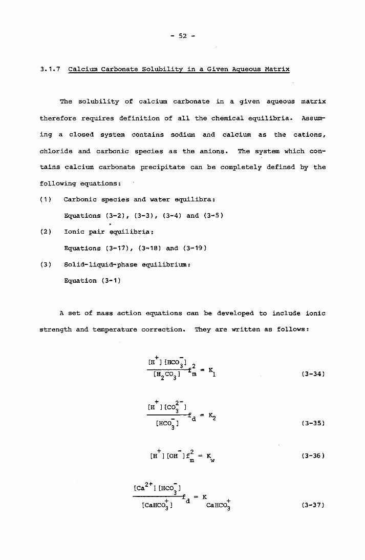
52
3.1.7 Calcium Carbonate Solubility in a Given Aqueous Matrix
The solubility of calcium carbonate in a given aqueous matrix
therefore requires definition of all the chemical equilibria. Assunt-
ing a closed system contains sodium and calcium as the cations,
chloride and carbonic species as the anions. The system which con
tains calcium carbonate precipitate can be completely defined by the
following equations:
(1) Carbonic species and water equilibra:
Equations (3-2), (3-3), (3-4) and (3-5)
(2) Ionic pair equilibria:
Equations (3-17), (3-18) and (3-19)
(3) Solid-liquid-phase equilibrium:
Equation (3-1)
A set of mass action equations can be developed to include ionic
strength and temperature correction. They are written as follows:
[H ][HC03] 2[H2C03] fm K1 (3-34)
[hco3] (3-35)
+[H ] [OH ]f (3-36)m w
[Ca2 + ] [HCO~]-----~----fd = K[CaHCO*] ( + (3-37)CaHC03
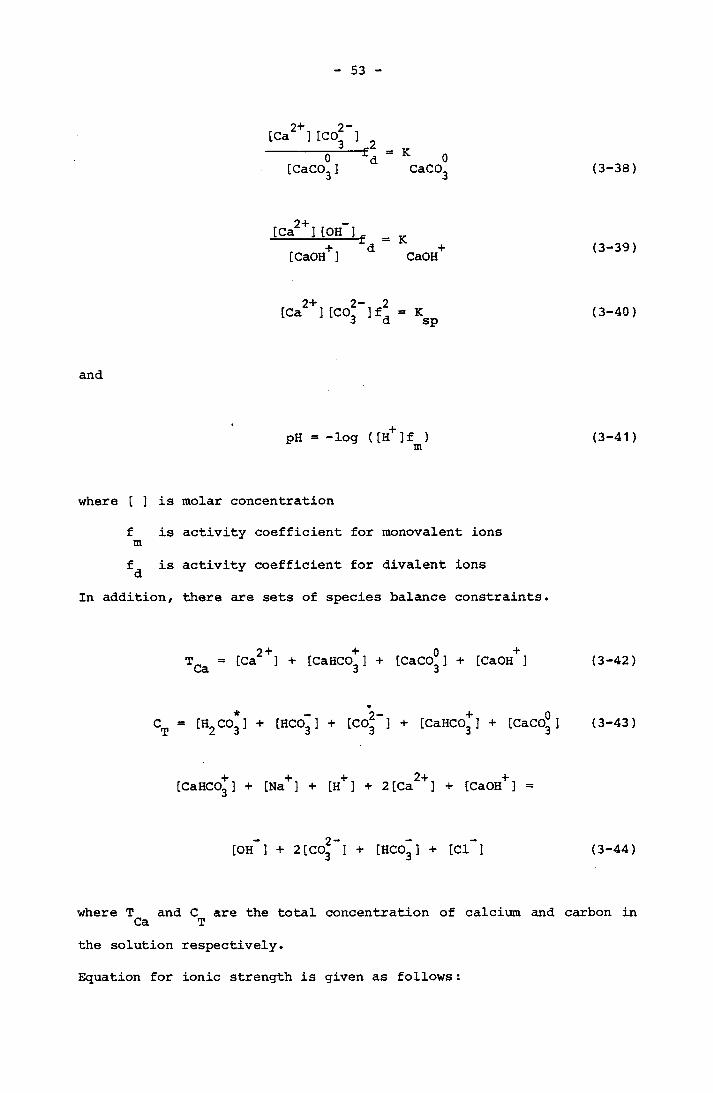
53
2+ 2 [Ca ][C030[CaC03] CaCO, (3-38)
[Ca2+][OH~l =+ d +[CaOH ] CaOH (3-39)
[Ca2+] [C02']f^ Ksp (3-40)
and
pH = -log ( [H+ ] f ) m (3-41)
where [ ] is molar concentration
f is activity coefficient for monovalent ions mf is activity coefficient for divalent ions d
In addition, there are sets of species balance constraints.
2+ + 0 +T = [Ca ] + [CaHCO ] + [CaCO 1 + [CaOH ] (3-42)U3. o o
* - 2- + 0 CT = [H2C031 + [HC03 ] + [C03 ] + [CaHC03 ] + [CaC03 ] (3-43)
[CaHCOg] + [Na+] + [H+] + 2[Ca2+] + [CaOH+] =
[OH ] + 2[CO2 ] + [HC03] + [Cl ] (3-44)
where T and C are the total concentration of calcium and carbon in Ca Tthe solution respectively.
Equation for ionic strength is given as follows:

54
I = 0.5([ H+ ] + [Na+] + 4[Ca2+] + [OH ] + 4[CO2 ] +
[HC03] + [Cl"] + [CaHCO*] + [CaOH+]) (3-45)
Activity coefficients of mono and divalent ions are calculated from
Equation (3-27).
The above equations allow calculation of the concentrations of
species distribution in the aqueous system. Water samples can be
analysed to determine the total concentration of cations and anions.
The pH value can be measured. Total carbon content can be determined
using an Inorganic carbon anaylyser (A.P.H.A-A.W.W.A.-W.P.C.F., 1980).
If an Inorganic carbon analyzer is not available, total alkalinity of*
the solution determined by H2C03 end P°i-nt titration can be used to calculate carbonic species distribution.
[Aik] = 2[CO2™] + [HCO™] + [OH™] - [H+] 3 3 (3-46)
[HCO’]— + [Aik] - [OH ] + [H ,]
(1 + 2K2/[H+]) (3-47)
[C°3~] [Aik] - [OH~] + [H+] ( [H+] A2 + 2) (3-48)
[H2C03][Aik] - [OH ] + [H ]
(K^/[H+] + 2K^/[H+]2) (3-49)
V Iwhere and are first and second dissociation constant of carbonic
acid with ionic strength correction.2+ 2-The product of the calculated [Ca ] and [CO^ ] of the system can be

55
used to describe the solubility of calcium carbonate.
3.2 COMPUTER PROGRAMMES
3.2.1 Programmes for Chemical Composition Calculation
3.2. 1.1 Pure Calcium Carbonate System (PROG-CS)
The chemical compositions of solution after mixing sodium bicar
bonate and calcium chloride can be calculated by the established
equilibria. The following assumptions are made for the calculation:
1. Chemical equilibria among dissolved species are established
instantaneously after mixing as compared to the equilibrium of2+ 2-calcium carbonate precipitate with [Ca ] and [CO^ ].
2. The contribution of [CaOH+] is insignificant below pH 10 as com
pared to [CaHCO*] and [CaCO^] (Wiechers and Sturrock, 1975).3. It was observed that solutions of sodium bicarbonate under exper
imental stirring rates maintained a constant pH. Therefore car
bon dioxide transfer between the liquid phase and the small gase
ous space in the enclosed stirred reactor used for calcium car
bonate precipitation experiments is insignificant (Chapter 4 ).
As a result, a closed system is adopted to describe the carbonic
species distribution.
A computer programme was established to calculate concentrations of
all relevant species in the solution by an iterative method. Subse
quently the degree of supersaturation, S, defined as:
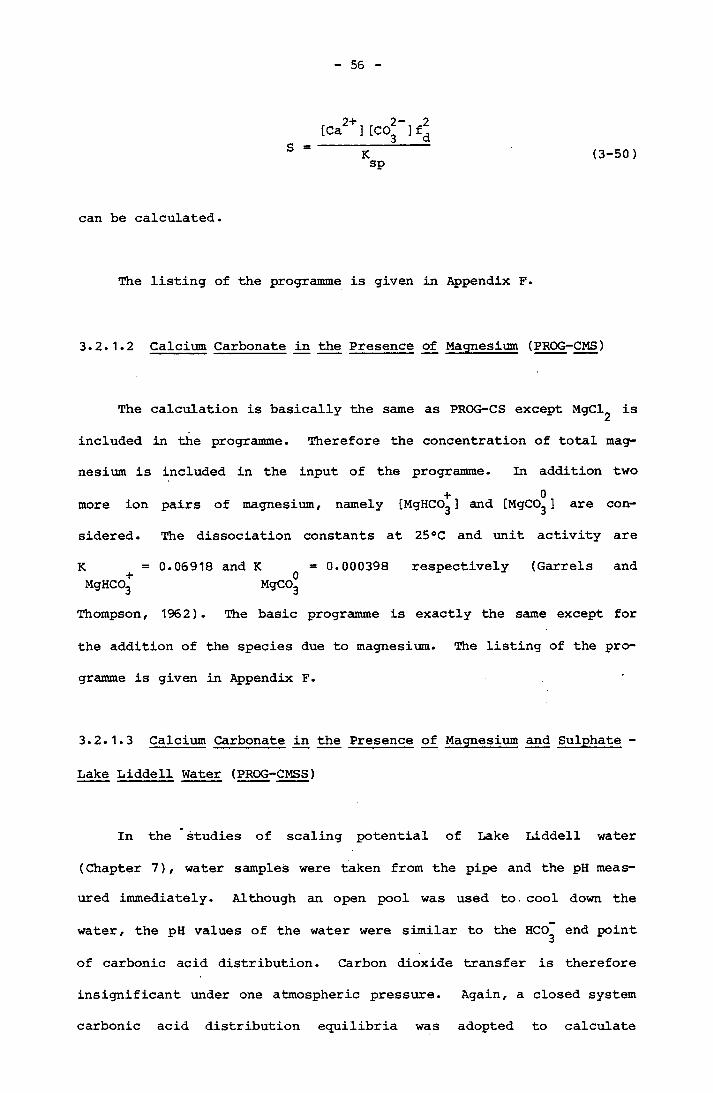
56
[Ca2+] [C02~]f2 ___ 3___ dK (3-50)sp
can be calculated.
The listing of the programme is given in Appendix F.
3.2.1.2 Calcium Carbonate in the Presence of Magnesium (PROG-CMS)
The calculation is basically the same as PROG-CS except MgCl^ is
included in the programme. Therefore the concentration of total mag
nesium is included in the input of the programme. In addition two+ 0more ion pairs of magnesium, namely [MgHCO^ ] and [MgC03 ] are con
sidered. The dissociation constants at 25°C and unit activity are
K = 0.06918 and K = 0.000398 respectively (Garrels andMgHC03 MgC03
Thompson, 1962). The basic programme is exactly the same except for
the addition of the species due to magnesium. The listing of the pro
gramme is given in Appendix F.
3.2.1.3 Calcium Carbonate in the Presence of Magnesium and Sulphate -
Lake Liddell Water (PROG-CMSS)
In the studies of scaling potential of Lake Liddell water
(Chapter 7), water samples were taken from the pipe and the pH meas
ured immediately. Although an open pool was used to cool down the
water, the pH values of the water were similar to the HCO^ end point
of carbonic acid distribution. Carbon dioxide transfer is therefore
insignificant under one atmospheric pressure. Again, a closed system
carbonic acid distribution equilibria was adopted to calculate
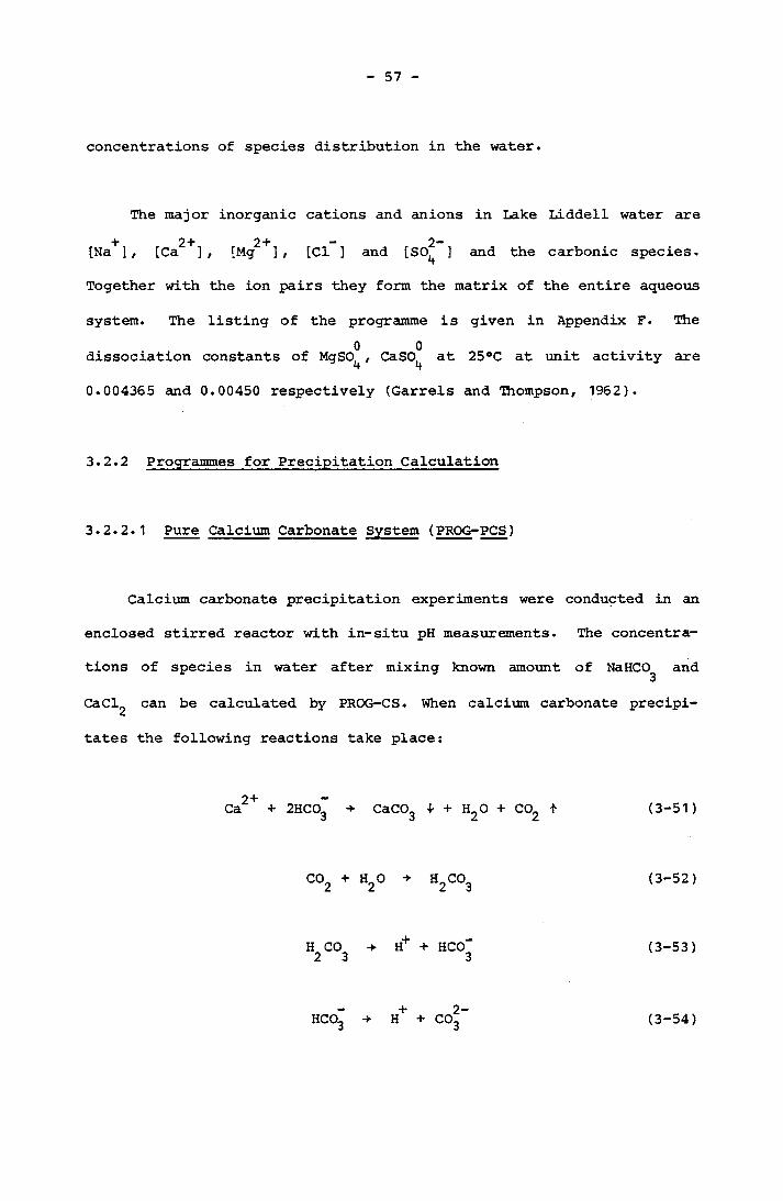
57
concentrations of species distribution in the water.
The major inorganic cations and anions in Lake Liddell water are+ 2+ 2+ 2- [Na ], [Ca ], [Mg ], [Cl ] and [SO^ ] and the carbonic species.
Together with the ion pairs they form the matrix of the entire aqueous
system. The listing of the programme is given in Appendix F. The0 0dissociation constants of MgSO, , CaSO at 25°C at unit activity are4 4
0.004365 and 0.00450 respectively (Garrels and Thompson, 1962).
3.2.2 Programmes for Precipitation Calculation
3.2.2.1 Pure Calcium Carbonate System (PROG-PCS)
Calcium carbonate precipitation experiments were conducted in an
enclosed stirred reactor with in-situ pH measurements. The concentra
tions of species in water after mixing known amount of NaHCO^ and
CaCl^ can be calculated by PROG-CS. When calcium carbonate precipi
tates the following reactions take place:
2+Ca + 2HC03 -* CaC03 + + H20 + C02 t (3-51)
co2 + h2o -► h2co3
H CO H+ + HCCf2 3 3
- + 2- HC03 -► H + C03
(3-52)
(3-53)
(3-54)
58
Therefore the nett result is a decrease in pH of the water. The
concentration of the species will distribute among themselves accord
ing to the chemical equilibria. A method to calculate species concen
tration during precipitation was given by Wiechers et. al. (1975).
The assumptions for PROG-CS are also applicable to the precipitation
process. Therefore the decrease in total calcium due to calcium car
bonate precipitation must be accompanied by a decrease in total car
bon.
ATCa = ACT (3-55)
i2+ + oT = ( [Ca ] . + [CaHCO ] . + [CaCC> ] . ) Ld X 3^. 3 1
( [Ca ] -1- LCaHC03 J + [CaCC>3 ] ) (3-56)
Cm = ( [H CO ] . + [HCO ] . + [CC> ]. + [CaHCO ] . T 2 3 1 3 1 3 1 3 12- +
i
2- + 0 + [C03 ] + [CaHC03 ] + [CaC03 ] ) (3-57)
where [ ] disignate initial molar concentrations at time, 9=0
[ ] designate molar concentrations at time 9.2+ 2-The supersaturation of the water is depicted by [Ca ] and [C03 ] .
2+ 2+Therefore the change of [Ca ] , ACa can be solved from Equations
(3-56) and (3-57)

59
* - 2-- ([H2C03] + [HC03] + [C03 ]) (3-58)
2+Applying the above equations, when [Ca ] is reduced by a finite qua-2+tity from the initial [Ca ] calculated from PROG-CS, the correspond
ing species concentration in the water can be recalculated again by an2+iterative method. Again the new [Ca ] can be reduced by this finite
quantity and the whole process repeated. Each calculation will also
calculate [H+ ] which can be converted to pH. Therefore from the pH
values measured in-situ during precipitation, the respective species
concentration distribution can be known and allows subsequent kinetic
derivation of the process. The listing is given in Appendix F. All
the input data are obtained from the initial species concentration
calculated by PROG-CS.
3.2.2.2 Calcium Carbonate in the presence of Magnesium (PROG-PCMS)
The initial concentrations can be calculated from PROG-CMS.
Similar principles apply except the additional terms due to the con
tribution of magnesium ion pairs to total carbon calculation:
- C UH2co3]. + [hco3], + [c°r]i+ o ++ [CaHCO ] . + [CaCO ] . + [MgHCO ] .3 i 3 l 3 x
+ [MgC03 ] ) - ([H2C03] + [HCO~ ] + [CO*”]
+ 0 +0 + [CaHC03] + [CaC03J + [MgHC03] + [MgCOg]) (3-59)
The listing of the programme is given in Appendix F.

60
CHAPTER 4
EXPERIMENTAL STUDIES OF PRECIPITATION OF CALCIUM CARBONATE
4.1 NUCLEATION AND CRYSTALLIZATION OF CALCIUM CARBONATE - A LITERATURE REVIEW
4.1.1 Introduction
The precipitation of calcium carbonate is an important phenomenon
in many process. Although the precipitation in water supplies and
cooling water systems, followed by subsequent build up of calcium car
bonate scale has been known in both domestic and industrial practice
for many years, there are many beneficial applications of calcium car
bonate. In water softening of potable water, precipitation of calcium
carbonate plays a vital role to remove hardness. Calcium carbonate is
also extensively used in industry as a filler for plastic materials,
rubber, paper etc. The control of the calcium carbonate precipitation
process, either to avoid scaling or for industrial application, there
fore has important implications. Consistent control of the process
can only be acheived with detailed understanding of the crystalliza
tion process of calcium carbonate, and this has become a substantial
research interest during the past decades.
61
4.1.2 Nucleation of Calcium Carbonate
The rate of nucleation is influenced by various factors in the
solution, such as the presence of heteronuclei and impurities, the
degree of supersaturation and the mixing energy. Truely homogeneous
nucleation of calcium carbonate is probably never observed, however
under a very high degree of supersaturation, the influence of
heteronuclei can be reduced to a minimum and the nucleation process is
approximately homogeneous. In all the studies reported in the litera
ture for calcium carbonate nucleation, rate of nucleation was measured
in terms of an experimentally measured induction period and this was
used to calculate the interfacial tension between calcium carbonate
nuclei and the solution. Roques and Girou (1974) studied calcium car
bonate crystallization by gasing the known concentration of calcium
carbonate solution with a constant stream of air/carbon dioxide mix
ture in which the partial pressure of carbon dioxide was equal to the
equilibrium pressure. Once the solution reached the desired tempera
ture, the supersaturation was created with air/carbon dioxide mixtures
of lower carbon dioxide partial pressure. The solution was stirred by
the gas. Appropriate stirring was achieved by adjusting the gas flow
rate. They also studied the process with mechanical stirring in addi
tion to gasing to create supersaturation. Three temperatures, namely
10°C,, 30°C and 50°C were studied. An empirical correlation between
the nucleation velocity and inital crystal growth velocity was given
as:
o•88VG = 1.22 x 10 VQ* at 30°C (4-1)
where V is the germination (nucleation velocity), minCj“1

62
Vg is the initial crystal growth velocity, mg/L min
All three types of calcium carbonate, namely vaterite, calcite and
aragonite were observed under the experimental conditions used. They
calculated the interfacial energies based on Volmer, Becker and
Dorring's classical formulae:
log T y G 1/log (degree of supersaturation) (4-2)
where T is the latency time (germination period) as defined. The Gresults are shown in Table (4-1).
TABLE 4-1
Values ofVariety of
Interfacial Energies Obtained
Calcium Carbonate (after Roque
for each
and Girou)
Temp. Aerated Mechanically
(°C) Vaterite Systems Aragonite agitated
Calcite Systems
Aragonite
2 210 15 MJ/m 3 MJ/m
30 214 MJ/m 27 MJ/m 27 MJ/m 27 MJ/m2 250 23 MJ/m 11 MJ/m
63
Germination (nucleation) was found to be influenced by the method
of gas bubbling employed to create supersaturation. It is believed
that heterogeneous nucleation was created under such condition.
Therefore this also explains the low values of interfacial energies
obtained in their experiments which are more than 10 times less than
the data obtained from other investigators (Sohnel and Mullin, 1978,
1982).
Sohnel and Mullin (1978,1982) used various methods to measure the
experimental induction period, which is the time taken for the first
measurable change of solute concentration in the form of turbidity,
conductivity or by simple observation with the naked eyes for the
first sign of crystals They developed a stopped-flow method (Sohnel
and Mullin, 1978) to detect the induction period by conductivity. The
principle of the stopped-flow method was already commonly used in
studying the kinetics of very fast reactions. This method could
detect induction periods as short as 5 ms which therefore enabled them
to study nucleation of calcium carbonate under very high degrees of
supersaturation. Under such high degree of supersaturation, hetero
geneous nucleation is negligible. Adopting the theory of Nielsen and
Sohnel (1971) derived for homogeneous nucleation based on the diffu-
sional growth of the created nuclei, the logarithm of induction period-2is a linear function of (logs) in the form:
2log9. = K „. + a./(logs )ind (4-3 ) t a
where K,(4-3 ) S is
is a constant
the degree of supersaturation based on activity
the gradient based on the induction period and
(4-3)
64
a, = 2p a3V2/5(KTln10)3 (4-4)t m
where {3 is a geometry shape factor
a is the interfacial energy
V is the mean ionic volume mK is the Boltzman constant
T is the absolute temperature in °K
Therefore a could be calculated from the gradient of the plot of-2logO. , versus (log S )ind a
From a microscopic count of the number of crystals in the precip
itation suspension it was found that the logarithm of number of cry--2stal per unit volume is a linear relationship to (logs) (Nielsen,
1967) in the form:
log N = k(4_5) " aN/(lo<?Sa)2 (4-5)
where K, v is a constant (4-5 )a is the gradient based on crystal number NN is the number of crystals per unit volume
and
3 5 3a V /5(KTlnl0) m (4-6)
The interfacial energies of calcium carbonate determined are 83 mJ/m2 2+(Sohnel and Mullin, 1978) , 98 and 107 mJ/m for the pure and Mn
contaminated systems respectively (Sohnel and Mullin, 1982).
65
The interfacial energy for calcite was calculated based on the
assumption of surface hydration which gave reasonable estimates of at
least 30 other substances (Nielsen and Sohnel, 1971). The value is
2120 rtvJ/m and obviously compared well with the above values. Other
2values have been reported in the literature, such as 7 mJ/m (Roques
2 2and Girou, 1974), 19.5 mJ/m (Kharim, 1974) 205 rrvJ/m (Moller and
2Rajogopalan, 1976 ) and 280 nvJ/m (Goujonand Mutaftschiev, 1976) for
2 2calcite, 10 mJ/m (Kharim, 1974) and 14 mJ/m (Roques and Girou, 1974)
2for vaterite and 150 rtvJ/m (Moller and Rajagopalan, 1976) for aragon
ite. Based upon the range of experimentally studies Sohnel and Mullin
(1982) made the following comments:
2Low values in the range of 7 - 20 mJ/m were due to heterogeneous
2nucleation. The extremely high value 280 mJ/m was derived from
2 , 2doubtful equations. The values of 205 nvJ/m and 150 mJ/m were
derived from experiments based on the assumption of polynuclear growth
however under the experimental conditions there was a strong possibil
ity of a spiral growth mechanism. Therefore it was concluded that the
2value 120 mJ/m for calcite was valid. Kharim et. al. (1980) also
2reported 110 rtvJ/m as the interfacial energy of calcium carbonate.
Impurities in the form of cations can affect the nucleation of
calcium carbonate. In general, cations having atomic radii smaller
than that of calcium and hydration energies higher than calcium are
capable of altering the crystal form from calcite to aragonite, simul
taneously the induction period is increased. This fact has been
reported frequently in the literature. Roques and Girou (1974)
observed an increase in induction period (latency time as they termed
it) with an increase in the concentration of magnesium. Moller and
66
Rajagopalan (1975) also observed the increase in induction period with
the increase in Mg/Ca ratio. They also reported there was a pronounced
discontinuity at Mg/Ca = 4 which indicated that beyond Mg/Ca = 4,
aragonite was formed. The nucleation rate of aragonite was lower than
calcite under similar conditions. Both papers reported the observation
under conditions of heterogeneous nucleation. Sohnel and Mullin
(1982) reported a similar trend of increasing induction period for an
increasing Mg/Ca ratio. The experiment was predominantly of homogene
ous nucleation. For the precipitation suspension with a degree of
super saturation less than 100 the number of crystals was less in the
presence of foreign cations (Mg, Mn) as compared to a pure system.
4.1.3 Crystallization of Calcium Carbonate
The early research work stemmed from a realisation of the impor
tance of the role played by calcium carbonate in geochemistry and
oceanography (Weyl, 1958; Pytkowicz 1965; Kitano et. al. 1962; 1965;
1966). Reddy and Nancollas (1971a, 1971b) avoided the possible com
plications caused by both the nucleation process during crystal growth
and heterogeneous nucleation. They conducted the study by using seed
crystals with known surface area in a supersaturated metastable solu
tion. The measured growth rate in terms of the rate of decrease in
total calcium concentration in the solution followed a second order
equation with respect to the concentration, this suggested a surface-
controlled process. The crystallization process was studied over tem
perature ranged from 10 to 40°C. The activation energy for crystal
growth was measured as 46.014.2 KJ/mole. The growth rate was indepen
dent on the stirring applied to the system. In their study, they pro
posed that the rate of calcium carbonate precipitation was the nett
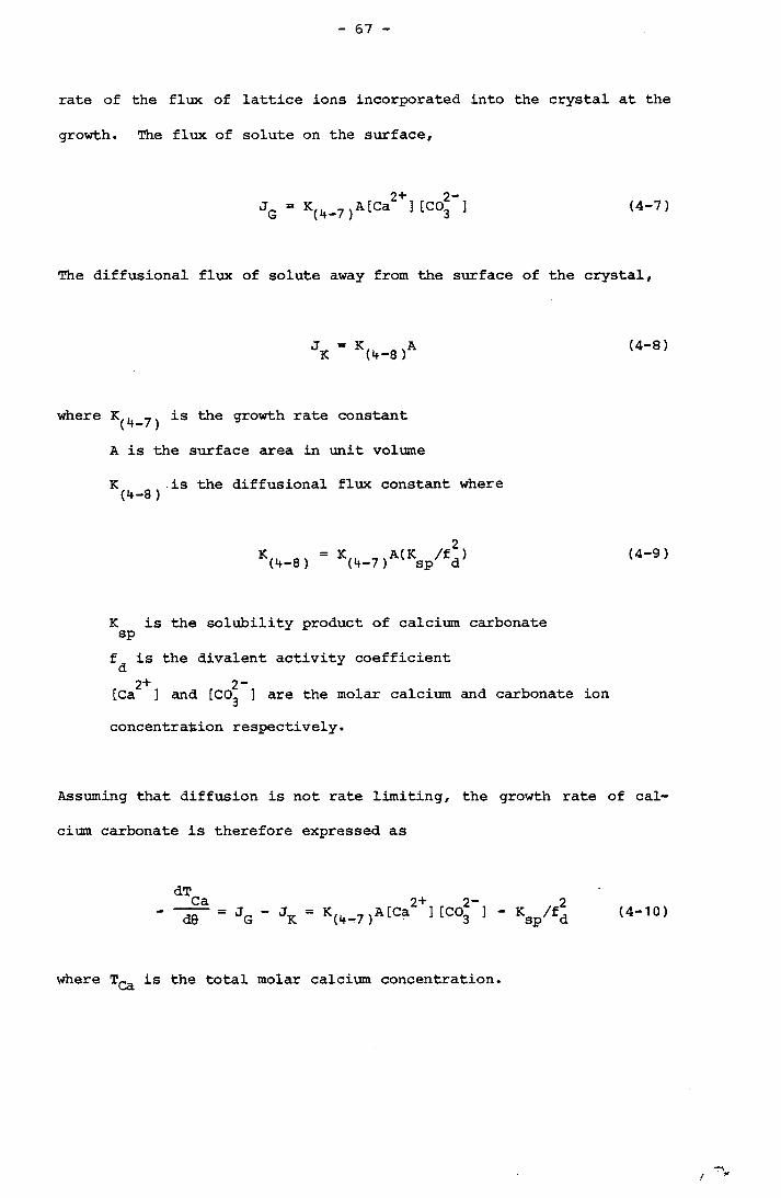
67
rate of the flux of lattice ions incorporated into the crystal at the
growth. The flux of solute on the surface,
2+ 2-K(4_?)A[Ca ] [C03 ] (4-7)
The diffusional flux of solute away from the surface of the crystal,
JK=K(4-B)A <4-8>
where K^4 ^ is the growth rate constant
A is the surface area in unit volume
K is the diffusional flux constant where(4-8 )
K(4-8) K 7.A(K /f2)(4-7) sp d (4-9)
K is the solubility product of calcium carbonate spf is the divalent activity coefficient
2+ 2“[Ca ] and [CO^ ] are the molar calcium and carbonate ion
concentration respectively.
Assuming that diffusion is not rate limiting, the growth rate of cal
cium carbonate is therefore expressed as
d9 K(4-7)A[Ca2+1[C03’) - Ksp/fd (4-10)
where T^ is the total molar calcium concentration.
/
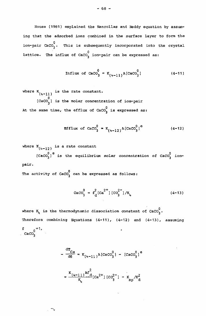
68
House (1981) explained the Nancollas and Reddy equation by assum
ing that the adsorbed ions combined in the surface layer to form the 0ion-pair CaCC>3• This is subsequently incorporated into the crystal
0lattice. The influx of CaCC>3 ion-pair can be expressed as:
0 0Influx of CaC03 = K4_lx)A[CaC03] (4-11)
where K is the rate constant.(4-11 )
0[CaC03] is the molar concentration of ion-pair0At the same time, the efflux of CaCC>3 is expressed as:
Efflux of CaCC>3 = K(j+_12 ^ A[CaC03 ]S (4-12)
where K ^ is a rate constant0 e 0[CaCC>3 ] is the equilibrium molar concentration of CaCO3 ion-
pair .0The activity of CaCC>3 can be expressed as follows:
0 22+ 2-CaCO = f [Ca ] [CO, ]/K (4-13)3d 3 4
0where is the thermodynamic dissociation constant of CaCC>3 .Therefore combining Equations (4-11), (4-12) and (4-13), assuming
f o=1'CaC03
d0 V-ina[CaC031 0 e[CaC03]
K, Af(4-11) ac 2+3 tco2- 3*4
K /K2 sp d
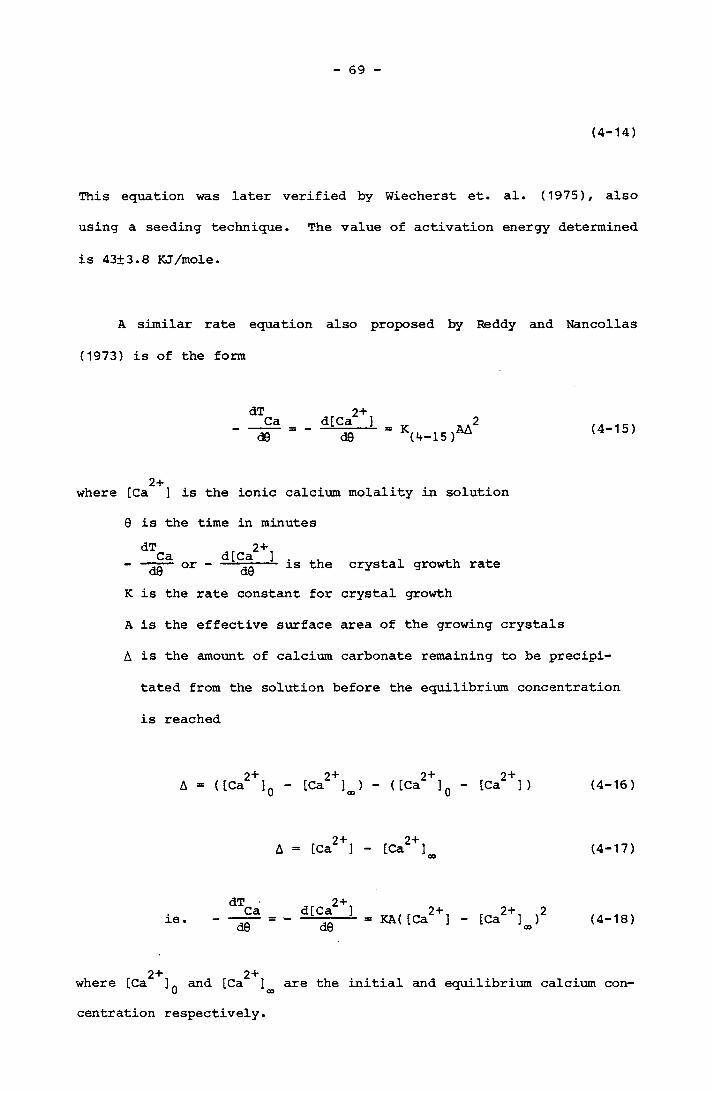
69
(4-14)
This equation was later verified by Wiecherst et. al. (1975), also
using a seeding technique. The value of activation energy determined
is 43±3.8 KJ/mole.
A similar rate equation also proposed by Reddy and Nancollas
(1973) is of the form
dT__Cad0
2+d[Ca ] d9 K(4-15)AA (4-15)
where [Ca ] is the ionic calcium molality in solution 9 is the time in minutes
dTc d C 2+]- or - -- is the crystal growth rateK is the rate constant for crystal growth
A is the effective surface area of the growing crystals
A is the amount of calcium carbonate remaining to be precipi
tated from the solution before the equilibrium concentration
is reached
A = ([Ca2+] - [Ca2+] ) - ([Ca2+]n - [Ca2+]) (4-16)U co U
2+ 2+ A = [Ca ] - [Ca ] (4-17)
dT 2 +Ca d[Ca ] 2+ 2+2ie. - —= - - —- ■ = KA( [Ca ] - [Ca ] )d0 de (4-18)
2+ 2 +where [Ca ] and [Ca ] are the initial and equilibrium calcium con-U oo
centration respectively.

70
The effect of some phosphonic acid derivatives was studied and
found that the rate of growth of calcite seed crystals was greatly
reduced. Equation (4-15) were also later adopted by Reddy to express
calcium carbonate crystallization (Reddy, 1977; Reddy and Wang, 1980;
Reddy and Gaillard, 1981).
Plummer et. al. (1978) studied the kinetics of semi-optical grade
crystals of Iceland spar dissolution at fixed values of P (0.0 to
1.0 atm.) and at temperatures which ranged from 5 to 60°C. When the
concentration is far from equilibrium, they identified that the rate
of dissolution consists of three forward rates:
1. First order dependence on the bulk fluid activity of H .
2. Linear dependence on the bulk fluid PF co2+3. A constant forward rate in the near absence of H and dissolved
CO .2
At near equilibrium, a backward reaction at constant P_^ and tempera
ture, was identified as the linear relationship of the product of the 2+ —activities of Ca and HCO^ in solution. As a result, the nett rate
Iof dissolution (R ) is given by an equation of the form:
R = k {H+} + k {H 2CO } + k {H 0} - k {Ca2+}{HCO } (4-19)1 2 s 3 3 2 4 3
where k^,k^,k^ are first order rate constants dependent of temperaturek is a function of both temperature and P 4 C02
*{H2CO^} which is the the carbon dioxide is equal to
{h2co3}+{co2>

71
{} indicates activity
Plummer et. al. (1978) used the adsorption layer heterogeneous
reaction model described by Mullin (1972) to derive their mechanistic
model. The adsorption layer model assumes a thin adsorption layer
between the surface of the crystal and the hydrodynamic boundary
layer. Species in the adsorption layer were assumed to have relative
low mobility as compared to species in the hydrodynamic layer. The
surface of the crystal is believed to be sparsely covered by reaction
sites at molecular-scale discontinuities in the surface. They also
assumed that forward and backward reactions involve kinetic interac
tion of boundary layer species and product species with the adsorption
layer species at the reaction sites. The following reactions were
considered to take place simultaneously:
+CaC03 + H (o) (4-20)
CaC03 + H2C03(o) - Ca ( g) + 2HC03 ( g} (4-21)
CaCO + H CL . -►3 2 (o) (4-22)
with the backward reactions:
HCO.3 (s)+ 2 H + CC>3 (s)
CaC03 + H+( s) (4-23)

72
2 +Ca + HCOo , s + HCOo , % -► CaCOo + H0CO, . , (4-24)3 (o) 3 ( s) 3 z 3 (s)
2 +Ca + HC00 . . + OH, . -* CaCO. + H„0, . (4-25)3 (o) (s) 3 2 (s)
where the subscript (s) and (o) indicate the species in the adsorption (surface) layer and at the bottom of the boundary layer respectively.
The form of Ca , and HCO^ involved in the backward reaction wasi 2+ — -not certain, therefore the notation Ca +HCCL , x was used. The3(o)
backward rates can be considered as the rate of crystallization as
against the rate of dissolution of calcium carbonate. Therefore these
nett rates of reactions from Equations (4-20) and (4-23), (4-21) and
(4-24), (4-22) and (4-25) are:
R1 ” k'<H+>(o) - k4{Ca2+}(o){HC03>(o) (4-26)
R2 “ k2{H2C°3>(o) * \,{Ca2+>(o){HC°3>(o){HC°3}(S) (4-27)
R3 - k3<H2°>(o) * \"{Ca2 + >(o){HC°3>(o){OH'}(s) (4-28)
tTotal dissolution rate (R ) is therefore
I I I 1R = R + R + R (4-29)12 3
At the high Reynolds numbers of their experiment, Plummer and Wigley
(1976) showed that bulk concentration is nearly equal to the concen
tration at the bottom of boundary layer, except for {H+} where pH is
less than or equal to 4. Also if reaction (4-20) is very rapid rela-*tive to reactions (4-21) and (4-22), (H CO }, . and {HO}, %2 3s(s) 1 2 (s) are both

73
equal to their bulk concentrations. For the application of calcium
carbonate precipitation, the approximation of {H+}, ={H+} in the bulk(s)
solution is not important because reaction (4-20) is negligible when
compared to the total rate at pH 7. At equilibrium,t I I
~ R2 = R3 = °* Rearranging the Equations (4-26) , (4-27) and (4-
28) by the substitution of K ,K ,K and K which are the dissociation1 2 sp wconstants of carbonic acid, the dissociation of bicarbonate, the solu
bility of calcium carbonate and the dissociation constant of water
respectively, the final form of k^ is
*2k4 = lkl + sp {H+> [k2{H2C03} ( S) + k2^H2°^(s)^
( s) (4-30)
To apply to calcium carbonate precipitation, substitute Equation (4-
30) into (4-19),
R = kL{H+} + k2{H2C03} + k3{H20} - {Ca2 + }{HC03} x r—^— +
1
{H+} [k {H CO*} , % - k {H 0} , 1'(s) 2 2 3; (s) 3 2 (s) (4-31 )
At low P ( <0.03 atm ) and pH greater than 7.0, k {H } andco2 1*
k2^H2^°3^ can neglected compared to k^f^O}. As a result, the rate
equation is approximated by
1 +Ca k,{H„0} ( (H ^ Q - 1)d® A 3'2-'-{h+}
(s) (4-32)

74
2+ 2“ {Ca^ }{Ca^ }where Q = ---- —------K.sp (4-33)
Therefore in order to use this rate equation, the surface pH value is
required. The dissolution experiments carried out by Plummer et. al.+(1978) were at relatively high P . The P and H are close toc^vj^ \ s)
+the bulk concentration due to the rapid reaction with H , therefore
the surface pH which is in equilibrium with calcite can be calculated
using an aqueous solution thermodynamic model, however this is not
true for precipitation at low P^ (Plummer et. al., 1979). The vali
dity of using this rate equation assuming that surface P and bulk
P^o are the same was tested by Reddy and Plummer (1981) and was shown
to be of restricted validity. Unfortunately, in order to calculate
the rate of calcium carbonate precipitation at low P^ ( <0.03 atm )
using a mechanistic model requires a value of surface P
House (1981) studied the kinetics of crystallization of calcite
from calcium bicarbonate solution using a seeding technique and adjusting the pH of the solution by bubbling a CO^/N^ gas mixture into
the metastable solution. He tested the available kinetic models with
the experimental data and concluded that the mechanistic model sug
gested Plummer et. al. (1978) gave the best fit to experimental data.
The growth model of Davies and Jones gave good agreement when the
extent of precipitation as defined in his paper (House, 1981) was
between 0.1 and 0.45. This Davies and Jones model was previously used
by Sturrock et. al. (1976) and Kazmlierczak (1979) and subsequently
used by House (1982). This equation is based upon a double-layer
model that allows for a difference in concentration of the adsorbed

75
ions and ions in the bulk of solution (Davies and Jones, 1955). The
potential set up between the crystal and bulk solution is such that
the concentrations of the cations and anions of the inorganic salt
taking part in the precipitation are equal in the monolayer. The
influx of cations and anions into the monolayer is proportional to
their concentrations at the surface of the monolayer. The efflux of
cations and ions from the monolayer is proportional to the solubility
of the inorganic salt in the aqueous solution. The nett influx of
cations and anions (ie. influx in excess of the efflux) equals the
flux available for precipitation. Applying Boltzman distribution law:
2 +Concentration of Ca in the monolayer 2+, - 2<\> /RT {Ca } e (4-34)
Concentration of CO^ in the monolayer = {CO^ }e+^(lJ/RT (4-35)3 3
2+ 2~where {Ca } and {CO^ } are the activities of calcium and carbonate in bulk solution
R is the gas constant
T is the temperature in °K
(J; is the potential difference between crystal and bulk solution
When the solution is saturated with calcium carbonate crystals,
in the monolayer,
/f 2+, -2c},/RT r 2-, 2(J,/RT ({Ca }e y ) ({CO. }e y ) = K3 sp (4-36)
therefore
{Ca2+}e'^/RT r 2”, 2(1;/RT 1/2{ C(J~ } e ^' = K3 so (4-37)

76
Thus for a saturated solution the influx (or efflux) of calcium and
carbonate are
Influx (or efflux) of Ca2+ 1/2K, . K
(4-38) sp(4-38)
Influx (or efflux) of CO.2- 1/2V-38)Ksp (4-39)
where K(4-38) is the rate constant.
2+If the supersaturated solution in which the concentration of Ca
2-is higher than CO^ , the potential defference, (|>, will be established
between the adsorbed layer and the bulk solution in such a way that
2+ 2-the concentrations of Ca and CO^ are equal at the monolayer sur
face. The influx of calcium and carbonate are
Influx of Ca2+ = K {Ca2+}e 2(^//RT (4-40)V H “ o O /
2- , 2“ 24>/RTInflux of C03 = K(4_38){C03 (4-41)
The efflux from the layer is given by Equations (4-38) and (4-39).
Therefore the nett fluxes are:
2+ - r 2+, -26/RT 1/2Nett flux of Ca = K^^g^-fCa }e - Kg^ ) (4-42)
2" r 2-4 26/RT 1/2Nett flux of CCT = K _ .({CO }e - K ) (4-43)3 (4 — 38) 3 sp
0The rate of formation of ion pair CaC(to be incorporated into the
2+ 2-crystal lattice) is proportional to the nett influx of Ca and CO^ .

77
Rate of formation of CaCO^/unit crystal surface =
r 2+, -26/RT 1/2 , 2“ 26/RT 1/2^({Ca }e - Kgp )({C03 }e - Kg? ) (4-44)
The rate of precipitation of calcium carbonate is proportional to the
rate of formation of CaCO^ and the total crystal surface area avail
able for growth, ie.
dTCa . , 2+, -26/RT 1/2.,, 2-, 26/RTIT “ V((Ca >e - KsP )<{co3 )e1/2K ) (4-45) sp
where A is the total crystal surface area in unit volume
K is the rate constant DJSince the concentration of calcium equals the concentration of car
bonate in the monolayer:
e2*/RT= ({ca2+}/{C02-})1/2 (4-45)
24;/RTSubstituting for e from Equation (4-46) to (4-45),
= K A({Ca2V/2{C02->1/2 - K1/Vd9 DJ 3 sp (4-47)
Incorporating activity coefficients,
d02 , 2+1/2 2-1/2 ; 2 1/2,2
KDJAfd{lCa 1 [C03 1 - (Ksp/fa > (4-48)
Sturrock, et. al. (1976) investigated the kinetics of calcium
carbonate precipitation in seeded batch experiments at 20°C. The
rates were expressed as a function of seed mass instead of surface
78
area and supersaturation by both the Nancollas and Reddy equation
(Equation (4-14)) and the Davies and Jones equation (Equation (4-48)).
The kinetic constants were found to be a function of the initial
supersaturation when applying the Nancollas and Reddy equation. This
suggested that the hypothesis of Nancollas and Reddy was not sus
tained. However, the kinetic constants were independent of initial
supersaturation when the Davies and Jones equation was applied. Stur-
rock et. al. (1976) concluded that the hypothesis of Davies and Jones
applied well for cacium carbonate precipitation.
Crystallization of calcium carbonate is influenced by many fac
tors such as the presence of heterogeneous nuclei, initial degree of
supersaturation, temperature and also the presence of foreign ions
which affect the size and morphology of the final crystals. Crystal
growth also is greatly reduced or completely inhibited in the presence
of some foreign ions. Studies on the effect of magnesium on calcium
carbonate crystallization have been published by many investigators
(Taft, 1967; Kitano, 1967; Roques and Girou, 1974; Reddy and Nancol
las, 1976; Reddy and Wang, 1980)^ Sufficient magnesium in the solu
tion tends to reduce the crystal growth rate and favours the formation
of aragonite rather than calcite. It was reported that at a concen-_3tration of 10 M magnesium ions the rate of crystallization was
-5greatly reduced, at 10 M of magnesium ions there was no effect
(Reddy and Wang, 1980). Besides magnesium, other metal ions such as 2+ 2+ 3+ 2+ 2 +Ni , Co , Fe , Zn and Cu also encourage the formation of ara-
2+ 2+ 2+ 2+ 2+gonite, while Mn , Cd , Sr , Pb and Ba favour calcite. In general, metal ions with a small ionic radius and higher hydration energy
2+than that of Ca result in aragonite formation (Roques and Girou,
1974).

79
The crystallization process is usually studied in a batch stirred
reactor, a continuous stirred reactor can be used to study the process
especially to acquire information for industrial crystallizer opera
tion. Calcium carbonate crystallization has been studied using con
tinuous stirred tank reactors (Maruscak et. al., 1971; Attarian et.
al., 1976; Schierholz and Stevens, 1975; Swinney and Stevens, 1982).
The studies investigated product size control and crystallization
kinetics. Schierholz et. al. (1975) used the population balance con
cept (Radolph and Larson, 1971) to investigate calcium carbonate cry-
stalization kinetics in a mixed suspension mixed product removal
(MSMPR) crystallizer which was applicable to water softening. Calcium
carbonate was precipitated out by continuously adding fixed concentra
tions of calcium sulphate and sodium carbonate reagents to the stirred
reactor, while a fixed quantity of mixed suspension was removed
periodicaly to maintain the required residence time. Calcite was found
to form at low residual supersaturation and aragonite at higher super
saturation. Crystallization was found to follow a power law model.
4.2 EXPERIMENTAL METHOD - A GENERAL SURVEY „
4.2.1 Nucleation Studies
4.2.1.1 Homogeneous Nucleation Studies
It is not unusual to find contradictory results on nucleation
studies reported in the literature. This is especially true when one
attempts to study homogeneous nucleation and fails to realise the
experimental problems involved becuase it is difficult if not impossi
ble to create a dust-free solution for homogeneous nucleation.
80
Furthermore, there are experimental difficulties because of the
extremely small size and fast rate of nuclei formation for homogeneous
nucleation. Some results reported on homogeneous nucleation were
believed to be distorted by the presence of impurities and hence were
really studies of heterogeneous nucleation. Homogeneous nucleation
has to be studied using dust-free solutions and then allowed to
proceed with the solution isolated from all possible contaminants both
from the atmosphere and from containers or equipment. These problems
were believed to be solved by Vonnegut (1948) who subdivided a liquid
system into a large number of tiny, non-communicating droplets whose
number greatly exceeded the number of impurities (foreign nuclei).
Therefore the impurities were only present in relative few droplets
and the effect was reduced to a minimum, hence reproducible rate meas
urements became possible. This principle was subsequently used and
further developed by other investigators (Pound and La Mer, 1952;
Turnbull, 1952; White and Frost, 1959; Melia and Moffitt, 1964;
Newkirk and Turnbull, 1955). An apparatus developed by White and
Frost (1959) was modified by Melia and Moffitt (1964) to study homo
geneous nucleation. This apparatus was designed to produce droplets
of aqueous solution suspended in oil. The aqueous solution was con
tained in a reservoir as a temperature above the saturation tempera
ture of the solute. The solution was allowed to flow from the reser
voir through the capillary jet and droplets were stripped off by the
flow of oil past the capillary tip. The size of the droplets could be
closely adjusted by the rate of flow of oil past the capillary tip and
coarsely adjusted by the dimentisons of the capillary. The tempera
ture of the oil below the tip was regulated by a thermostatically-
controlled flowing water jacket. The temperature could be set at
below the saturation temperature of the solution to cause nucleation.

81
Furthermore the composition of the oil could be arranged to solidify
at that temperaure. As a result, the droplets, about 100 - 200 in a
typical run could be fixed and observed over long periods of time.
The droplets could be observed with a microscope fitted with crossed
Nicol prisms to detect the presence of crystallization. Therefore the
percentage of droplet nucleate with respect to time could be followed.
However this technique has it shortcomings:
1. The number of crystal formed in the droplets cannot be counted,
2. The beginning of nucleation of sparingly soluble salts and sats
with a low temperature-coefficient of solubility cannot be
detected visually because only a small amount of precipitate
forms.
Melia suggested that these problems could be overcome by the method
similar to that used by Newkirk and Turbull (1955). They developed a
method to allow microscopic observation and to take photographs during
the course of nucleation and crystal growth. They dispersed the aque
ous solution into many small drops in warm liquid paraffin or silicone
oil by rapid mixing with a stirrer and a draught tube. A drop of this
dispersion was placed on a glass slide covered with a thin glass cover
slip and then examined on a special microscope stage whose temperature
was adjustable and controlled. Nucleation of solute could be trig
gered by cooling of the emulsion so that the solute saturation was
exceeded. The under cooling required to form crystals in the droplet
was detected to the accuracy of ±2°C and the supersaturation created
corresponds to or is nearly equal to the critical supersaturation for
homogeneous nucleation. Therefore the solute interfacial energy can
be calculated.

82
4.2. 1.2 Metastable Zone Width
Nyvlt (1968) suggested a method to study kinetics of nucleation
by measuring the width of the metastable zone of concentrations. When
supersaturation corresponds to the labile zone of the solute, the
nucleation rate increases rapidly. However, if solute supersaturation
is gradually achieved by moderate cooling, it is practically impossi
ble to exceed the limit of metastable supersaturation. Accoring to
Nyvlt's reasoning, the nucleation rate at the beginning of nucleation
should be identical for a limited period of time, therefore the
nucleation rate can be expressed in the form:
J nK P. n 1i i
K b (4-49)
where J is the mass nucleation ratem is the mass of crystals of size z which do not redissolve z
into
solution
d0 is the period of time during which the mass is formed
is the metastable zone width which is the difference in meta
stable limit concentration and equilibrium concentration of the solute
K and n are the nucleation rate constant and nucleation order nrespectively
IK represents the weight of the substance precipitated by a
unit volume of saturated solution by 1°CI
b is the cooling ratetIn addition, K can be expressed as
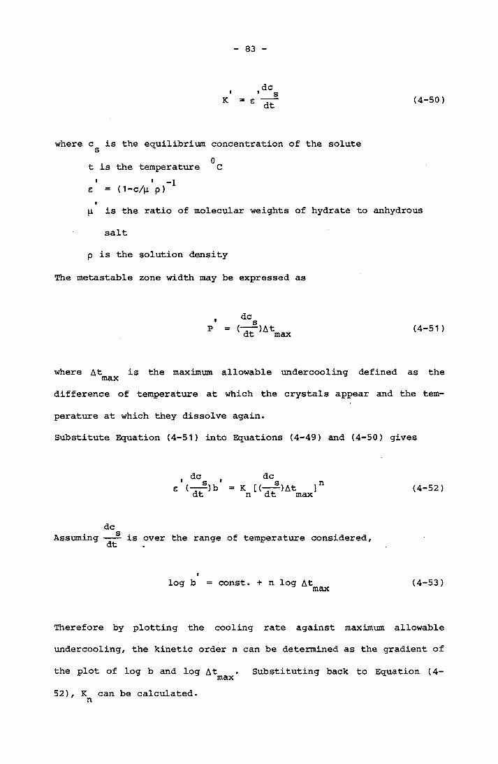
83
Kdc
(4-50 )
where c is the equilibrium concentration of the solute0t is the temperature C
' ' -1£ = ( 1 — c/|A p)I
p is the ratio of molecular weights of hydrate to anhydrous
salt
p is the solution density
The metastable zone width may be expressed as
P (—)At dt max (4-51)
where At is the maximum allowable undercooling defined as the maxdifference of temperature at which the crystals appear and the tem
perature at which they dissolve again.
Substitute Equation (4-51) into Equations (4-49) and (4-50) gives
£dc
K [(—-)At ]nn dt max (4-52)
dc 5Assuming --- is over the range of temperature considered,dt
log b = const. + n log Atmax (4-53)
Therefore by plotting the cooling rate against maximum allowable
undercooling, the kinetic order n can be determined as the gradient of
the plot of log b and log At . Substituting back to Equation (4-
52), K can be calculated, n

84
The experimental technique is relatively simple, a solution of
known saturation temperature is agitated and cooled at a specified
rate in a 50 mL Erlenmeyer flask and the temperature at which nuclei
first appear is recorded. The difference between the saturation and
nucleation temperature is the maximum allowable undercooling, Atmax,
for the particular cooling rate, b. This method was applied by some
investigators to study the nucleation of salts from solution (Mullin
and Osman, 1973; Mullin and Ang, 1977). In theory the metastable zone
width method proposed by Nyvlt is applicable to both homogeneous and
heterogeneous nucleation. However, the experimental setup proposed
invariably involved difficulties in providing dust-free solution for
true homogeneous nucleation. Therefore, the results obtained by using
this method apply to heterogeneous nucleation, which is evident in the
investigation by Mullin and Ang (1977). If the same principle is
applied to the Newkirk and Turbull method as described previously, it
is possible to investigate homogeneous nucleation.
4.2.1.3 Induction Period Method
Another completely different approach to nucleation study is by
mesasurement of induction period. A number of authors (Turnbull,
1953; Khamskii, 1969; Mullin and Osman, 1973) made simplifying assump
tions to suggest that the induction period was basically the time
involved in nucleation. Therefore, it was inversely proportional to
the rate of nucleation:
j = k e"1(4-54) ind (4-54)
where J is the number rate of nucleation

85
K is a constant of proportionality(4-54 )Based on the classical nucleation relationship ( see Equation (2-13)),
log(^—) « (—— --- ”}ind T (log S) (4-55)
-2Therefore the plot of log 0 ^ versus (log S) should result a
straight line and the gradient allows a, the interfacial energy to be
calculated. Under very high degrees of supersaturation, the induction
period is very small, but this is the situation where homogeneous
nucleation is more likely to take place because very high concentra
tions of nuclei are generated and the conditions minimize the influ
ence of heteronuclei. Therefore, to measure a very short induction
period becomes the major experimental difficulty. The simplest way to
measure induction period is by direct visual observation under a beam
of strong light. Two reagents required to produce the precipitate are
mixed rapidly into a beaker with a magnetic stirrer mixing the beaker
contents. The time taken for the first appearance of shiny crystals
is taken as the induction period. The first change of physical pro
perty, such as conductivity can also be taken as the induction. This
presents no problems if the induction period is longer than 5 seconds,
but under conditions of very high degrees of supersaturation, the
induction period is normally less than 5 seconds, in fact it is in the
range of milliseconds. This direct simple method becomes unsuitable.
Nielsen (1967) had devised a modified stopped- flow method by forcing
the reacting solutions into a mixing chamber of the Roughton type and
the mixture flows into an illuminated outlet channel. The induction
period was measured by means of a record on a 35 mm film moved con
tinuously at 50 cm per second in a Shackmann Oscilloscope Camera. At

86
low supersaturation, the induction period was measured as the time
that passed from the moment the pistons stopped to the appearance of a
visible precipitate. At high supersaturation, the length of the clear
zone between the mixing chamber and the place in the outflow channel
where the precipitate became visible was measured and converted to
induction period.
Sohnel and Mullin (1978) used Nielsen's stopped-flow and mixing
apparatus to measure the induction period by detecting changes of con
ductivity with a storage oscilloscope. The apparatus permitted time
measurements from 10 s to 1 ^,s. The oscilloscope sweep was triggered
when the flow of solution stopped, ie. mixing was completed. The
mixed solution than flowed backward and the period of conductivity
'steadiness' was therefore the induction period. This method detects
induction periods as short as 5 ms.
4.2.2 Crystallization Studies
4.2.2.1 Conventional Methods
Numerous experimental methods have been used to measure cry
stal growth rate. Since the growth rate of crystals can be described
by face growth rates of a single crystal as well as overall growth
rate on single and multi crystals, each method used is designed to
provide information only on certain aspects of crystal growth. These
methods include direct microscopic observation, photography and inter
ferometry to study single crystal face growth rate. The face growth
rate of single crystals is generally expressed in the empirical form:
87
n (4-56)
where G is the linear growth rate, length per unit time
A=C-C where C is the solute concentration and C is thes sequilibrium saturation
K(4-56) is the constant dependent on the velocity of the fluid
n is the order with respect to supersaturation
Alternately a much more convenient way of measuring crystal
growth is to determine the overall growth rate which is the mass depo-
sisted per unit time per unit surface ar-ea of the crystal. This is
especially useful for a multiparticle system. It can be studied in a
fluidised bed or in a batch stirred reactor from a known quantity of
seed crystals. It is also common to study the crystallization process
in a batch stirred reactor without separate seed addition. In such
experiments the precipitation of the crystals stems from nucleation
(O'Rourke and Johnson, 1955; Ang and Mullin, 1979; Konak, 1971; Sohnel
and Mullin, 1982). The empirical form of the overall growth rate
expression is:
where R is the overal growth rate and K is the overall growth rate G Gconstant.
When growth rate is also a function of crystal size, then
n (4-57)rg = kgac
R = KG (4-58 ) (4-58)
(4-58)where K and m are constants and L is the mean crystal size.

88
4.2.2.2 Population Balance by MSMPR Crystallizer
A completely different approach to study the kinetics of crystal
growth is by the population balance method. Kinetic data is best
obtained from a continuous mixed suspension mixed product remover
(MSMPR) crystallizer, where a stirred reactor is continuously fed with
precipitating reagents and the suspension in the reactor is intermit
tently removed to maintain a specified residence time. Information
obtained is applied to industrial crystallizer design to provide
required product size and yield. The concept of population balance
was first proposed by Randolph (1964) and Hulburt, et. al. (1964) to
describe the crystal size distribution (CSD) in a system. The
detailed mathematical treatment is given in the reference (Randolph
and Larson, 1971). In a MSMPR crystallizer, some assumptions are
made:
1. Steady state operation.
2. Perfect mixing.
3. No attrition of the particles.
4. Uniform shape factor.
The distribution of crystal sizes is represented in terms of
population density N, defined as
AN / ndL (4-59)
where AN is the number of crystals in size range to per unit
volume of suspension
89
n is a function of L
When the system is operating at steady state, the number rate of
crystals entering a size range must be equal to the number rate leav-
ing. Therefore, in an incremental time A9 / the number of crystals
entering size 1^ to because of growth is:
Vn G A0 (4-60)
where n is the population density of
is the linear growth rate of crystals of size
The number of crystals leaving size range to because of growth
is
Vn2G2A0 (4-61)
If the feed stream contains seed crystals in this range, then the
input to the distribution in the volume V is
' Q.n.ALA0 (4-62)i i
where Q. is the volumetric flow ratei
n is the average population density in the size range, ial=l2-lx.
Similarly, the withdrawal stream particles in the size range is
QnALA0 (4-63)
At steady state, input = output, therefore
90
Q.n AIA0 + VG n A0 = QnALA0 + VG n A0 11 11 2 2 (4-64)
rearranging,
V(Gn - G n ) = (Q n - Qn)AL 2 2 11 i i (4-65)
when L ■+■ 0A
Vd(Gn) Qn. - Qnl (4-66)
assuming there are no crystals in the feed stream n_^=0, then
(V)d(Gn) + n = QQ dL (44-67)
Assuming McCabe's AL law holds, ie. the growth rate is independent ofVcrystal size, also defining 9 = —, which is the residence time of the
drawdown time, the equation becomes
dnG6(—) + n = 0 (4-68)
Integrating Equation (4-68), and letting n be the population density
of zero-size crystals (the nuclei population density),
rn dn _ ,LdL J n„ n ' OG0 (4-69)
n = n exp(-L/G0) (4-70)
Therefore the plot of log n versus L gives a straight line with an0 -1intercept at L=0 equal to n and a gradient of Therefore G the
91
linear growth rate can be determined with known residence time of the
crystallizer.
Kinetics of nucleation and crystal growth can also be calculated
by the following equations:
0dNd0 + K(4-71)AC
where is the rate of nucleation.
G dLd0 K(4-72) Ac*
(4-71)
(4-72)
Now
0dN _ dNi _ dN* dL 0d0 ” d0 * L=0 ~ dL» L=0 d0 “ n (4-73)
Therefore
3sl = K am/ld0 (4-74 ) (4-74)
or
0nmT " 1
K(4-75 )G (4-75)
Therefore a plot of log n versus log G gives a straight line of gradient j - 1 . If l is known from the empirical equation of power law
of supersaturation, m may be evaluated for the kinetic order ofnucleation.
92
4.3 INTERPRETATION OF DESUPERSATURATION CURVE
A single batch crystallization experiment can conveniently gen
erate crystal growth data covering a wide range of degrees of supersa
turation. The solute concentration with respect to time can be fol
lowed by measuring parameters such as conductivity, refractive index
and pH of the solution. The resulting plot of concentration against
time is known as the desupersaturation curve of crystallization. A
typical desupersaturation curve is shown in Figure (4-1).
At point A, 0=0, supersaturation is created and is followed by a
period of nucleation. At point B, visible nuclei are formed and the
time taken is called the induction period, 0. . The mass precipi-mdtated out from the solution at this point is still insignificant to
cause a decrease in the measured solute concentration. However, the
precipitation process proceeds until the measured concentration begins
to decrease. This occurs at point C and the time taken is called theI
latent period. The solute concentration continues to experience a
steep decline where point C' represents the commencement of this steep
decline. This decline gradually slows down as indicated by region D
and E in Figure (4-1). Such a plot based upon a carefully controlled
batch experiment can give information about the kinetics of crystalli
zation. Methods are available to retrieve kinetic data from such
experiments and they are discussed below:

SOLU
TIO
N CO
NC
EN
TRA
TIO
N
92 a
~-|-----TIME
FIGURE 4-1 A Typical Desupersaturation Curve;cg = Equilibrium Saturation, =Induction Period, 0_ . = Latent Periodlat(after Mullin, 1972)

93
4.3.1 Chronomal Analysis
Chronomal (short term for chronometric integral) analysis was
first used by O'Rourke and Johnson (1955), the Chronomal, I,
corresponding to an assumed curve, can be plotted against time. A
straight line plot therefore confirms the growth law assumed. Nielsen
(1955,1964)) applied this technique to the precipitation process for a
range of compounds. Crystal growth mechanisms such as diffusion con
trol, surface nucleation control as defined by Nielsen can be identi
fied with this method. There are some major assumptions when applying
this method;
1. The crystals have identical size and shape.
2. The crystals retain their initial shape during growth.
3. Supersaturation is generated only at the beginning of an experi
ment.
4. No growth dispersion occurs.
5. No nucleation occurs during an experiment (ie. number of nuclei
is fixed).
With the above assumptions, the kinetics of crystallization can
be determined as follows:
Assuming empirical linear growth rate
dLd0 K a(4-76) (4-76)
where L is the characteristic length of the crystalc-cs
a is the supersaturation defined as -----c sc is the solute concentration at any given time
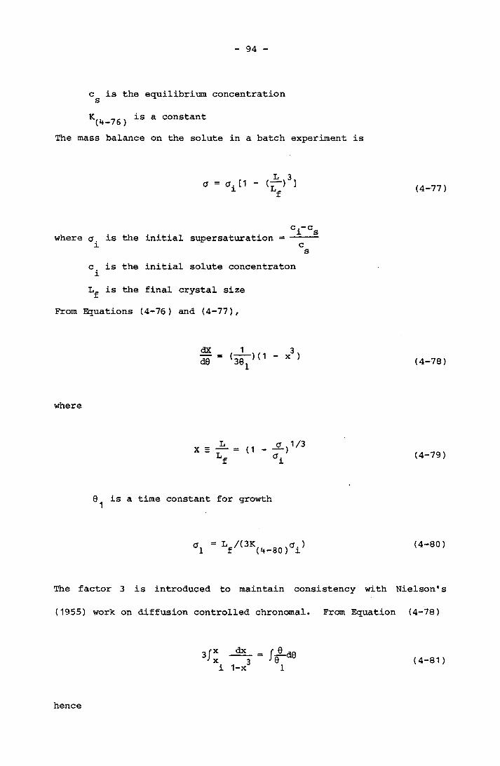
94
c is the equilibrium concentration
K,, . is a constant(4-76 )The mass balance on the solute in a batch experiment is
a = o’i [1
ci-cswhere a is the initial supersaturation = -----i cs
c _ is the initial solute concentraton
is the final crystal size
From Equations (4-76) and (4-77),
dXd0 (i?7)(1 X3 )
(4-77)
(4-78)
where
X = L(1
_d } V3 a. (4-79)
01
is a time constant for growth
L /(3K a )f (4-80) l (4-80)
The factor 3 is introduced to maintain consistency with Nielson's
(1955) work on diffusion controlled chronomal. From Equation (4-78)
3/xx
dx1—x~ 1 (4-81)
hence

95
I (x) - I (x.) = — 1 1 1 9i (4-82)
where I^(x) is the first order chromonal
h -x dx0 , 31-x
_1, , 1-x
(1-X)J.ln{ --} + / 3tan 1 (2^X-X) (4-83)
Therefore if the plot of 1^ (x) against time is a straight line, the
first order growth rate holds. The gradient is equal to 0 . If
and L are known, the growth constant K „ can be calculated, f * (4-79)Similarly, an empirical equation in the form of mth order kinet
ics
dLd0 c am (4-84)
I (x) m I (x. ) m i (4-85)
where 9 = L /(3C a^)m f mi
Im 3 m (1-x ) (4-86)
Again, a straight line plot confirms the empirical growth law and the
growth constant can be calculated from 9 provided L and a arem f iknown.

96
4.3.2 Turnbull's Characteristic Curve
Turnbull (1953) published his work on the kinetics of precipita
tion of barium sulphate. He defined the fraction of barium sulphatec -c
precipitated in time 9 by x = ----- where x is a function of time. Hec. -c x splotted the curve of x against time for different initial supersatura
tion experiments. When he applied a suitable scaling factor, he
noticed that all data fell onto a single characteristic curve
described by the general relations:
supersaturation. Equation (4-87) also can be written in the form:
where 0 is the time constant similar to that described in Section
(4-3-1). Turnbull reported that the rate of linear growth of barium
sulphate was independent of crystal size at the earliest stage of pre
cipitation. After the crystals reached a certain size their growth
rate became limited by diffusion. Therefore the linear growth rate
can be expressed in the form:
x = f ( ,9 ) (4-87)
(4-88)
B
(4-89)
where a , a and b are constants. If the expression of chronomal
analysis is used,
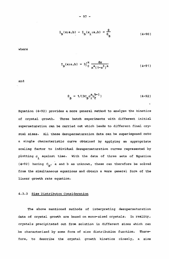
97
I (x;a,b) - I (x.;a,b) = B B i (4-90 )
where
IB(x;a/b) x dx(4-91)
and
(4-92)
Equation (4-92) provides a more general method to analyse the kinetics
of crystal growth. Three batch experiments with different initial
supersaturation can be carried out which leads to different final cry
stal sizes. All these desupersaturation data can be superimposed onto
a single characteristic curve obtained by applying an appropriate
scaling factor to individual desupersaturation curves represented by
plotting a. against time. With the data of three sets of Equation
(4-92) having C , a and b as unknown, these can therefore be solved Bfrom the simultaneous equations and obtain a more general form of the
linear growth rate equation.
4.3.3 Size Distributon Consideration
The above mentioned methods of interpreting desupersaturation
data of crystal growth are based on mono-sized crystals. In reality,
crystals precipitated out from solution in different sizes which can
be characterised by some form of size distribution function. There
fore, to describe the crystal growth kinetics closely, a size
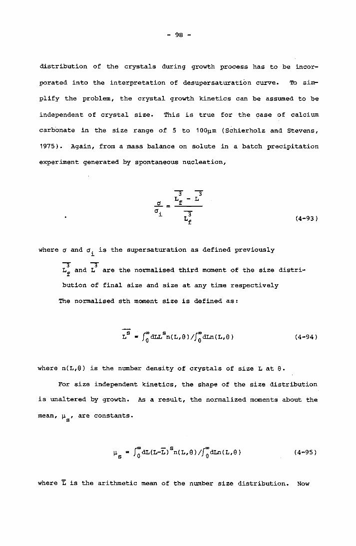
98
distribution of the crystals during growth process has to be incor
porated into the interpretation of desupersaturation curve. To sim
plify the problem, the crystal growth kinetics can be assumed to be
independent of crystal size. This is true for the case of calcium
carbonate in the size range of 5 to 100p,m (Schierholz and Stevens,
1975). Again, from a mass balance on solute in a batch precipitation
experiment generated by spontaneous nucleation,
(4-93)
where a and a. isi the supersaturation as defined previously
T Tand L are the normalised third moment of the size distribution of final size and size at any time respectively
The normalised sth moment size is defined as:
LS = /“ dLLSn(L,9)//“dLn(L,0) (4-94)
where n(L,0) is the number density of crystals of size L at 9.
For size independent kinetics, the shape of the size distribution is unaltered by growth. As a result, the normalized moments about the
mean, p, , are constants.
\i = f“dL(L-L)Sn(L,0)/j“dLn(L,0) (4-95)
where L is the arithmetic mean of the number size distribution. Now
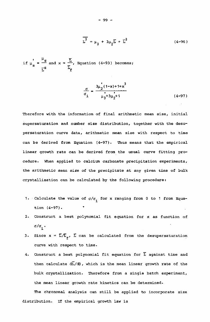
99
L3 = ^3 + 3^2L + L3
1 “ S Lif |i = — and x = —, Equation (4-93) becomes; S LS Ef
(4-96 )
' 33|i2 (1-x)+1 + x
ai ^3+3^2+1 (4-97)
Therefore with the information of final arithmetic mean size, initial
supersaturation and number size distribution, together with the desu
persaturation curve data, arithmetic mean size with respect to time
can be derived from Equation (4-97). Thus means that the empirical
linear growth rate can be derived from the usual curve fitting pro
cedure. When applied to calcium carbonate precipitation experiments,
the arithmetic mean size of the precipitate at any given time of bulk
crystallization can be calculated by the following procedure:
1. Calculate the value of a/a. for x ranging from 0 to 1 from Equa
tion (4-97).
2. Construct a best polynomial fit equation for x as function of
a/a. .i
3. Since x = L/L^, L can be calculated from the desupersaturation
curve with respect to time.
4. Construct a best polynomial fit equation for L against time and
then calculate dL/d0, which is the mean linear growth rate of the
bulk crystallization. Therefore from a single batch experiment,
the mean linear growth rate kinetics can be determined.
The chronomal analysis can still be applied to incorporate size
distribution. If the empirical growth law is
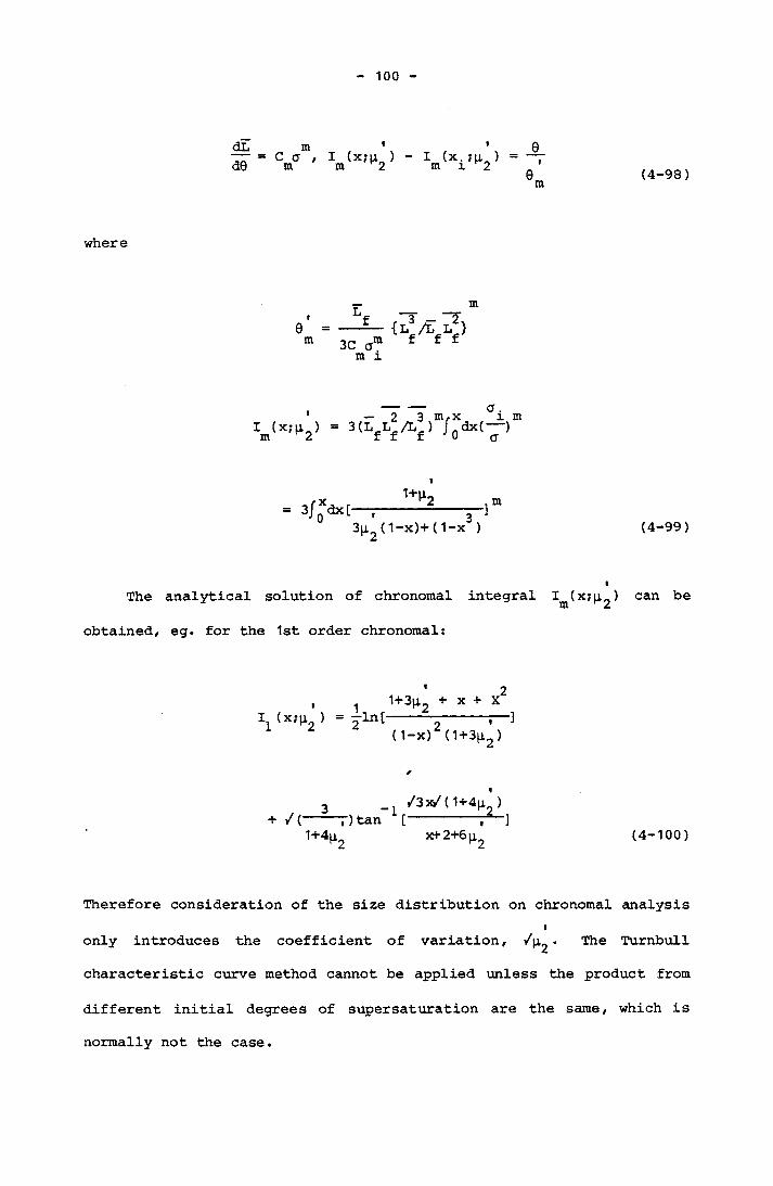
100
dLd0 Cma ' 1 JX»M ” Im(xi;^lo)m m 2 m i 2
9
9 m (4-98)
where
_i T __ T
0 = ----- {LA L }m 3C am f f f m i
' — 2 3 m,x i mI (x; (j, ) = 3 (L L /L ) J dx(—) m 2 f f f 0 a
3/^dx [-- r1+|l,
0 L ' 33ji (1-x)+(1-x ) (4-99)
The analytical solution of chronomal integral I^tx;^) can be
obtained, eg. for the 1st order chronomal:
' 2, , 1+3^2 + x + XVX'V = 2ln[(1 2.. ,( 1 — x) (1+3(i2)
3 /3x/(1 + 4|x )+ /(-----T) tan A[--------- , ]
1+4|i, x+2+6 ji. (4-100)
Therefore consideration of the size distribution on chronomal analysisI
only introduces the coefficient of variation, . The Turnbull
characteristic curve method cannot be applied unless the product from
different initial degrees of supersaturation are the same, which is
normally not the case.
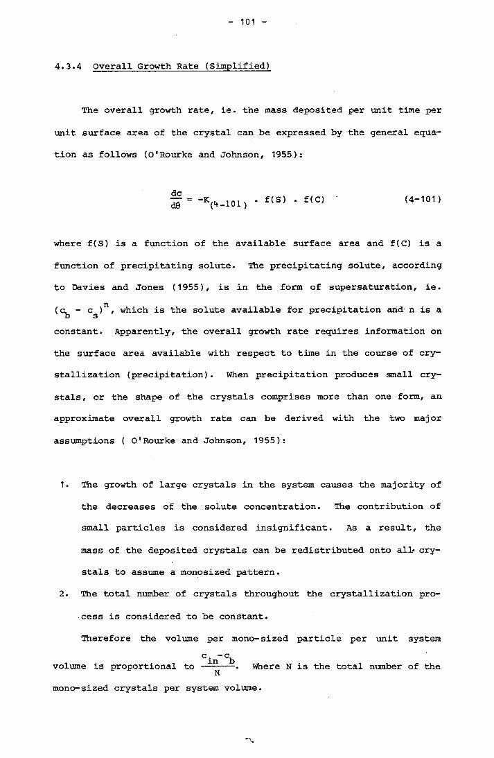
101
4.3.4 Overall Growth Rate (Simplified)
The overall growth rate, ie. the mass deposited per unit time per
unit surface area of the crystal can be expressed by the general equa
tion as follows (O'Rourke and Johnson, 1955):
dc _d0 = ’V-101) f(S) . f(C) (4-101 )
where f(S) is a function of the available surface area and f(C) is a
function of precipitating solute. The precipitating solute, according
to Davies and Jones (1955), is in the form of super saturation, ie.
(c, - c )n, which is the solute available for precipitation and n is a b sconstant. Apparently, the overall growth rate requires information on
the surface area available with respect to time in the course of cry
stallization (precipitation). When precipitation produces small cry
stals, or the shape of the crystals comprises more than one form, an
approximate overall growth rate can be derived with the two major
assumptions ( O'Rourke and Johnson, 1955):
1. The growth of large crystals in the system causes the majority of
the decreases of the solute concentration. The contribution of
small particles is considered insignificant. As a result, the
mass of the deposited crystals can be redistributed onto all- cry
stals to assume a monosized pattern.
2. The total number of crystals throughout the crystallization pro
cess is considered to be constant.
Therefore the volume per mono-sized particle per unit system
Cin~Cbvolume is proportional to -- —-- . Where N is the total number of the
mono-sized crystals per system volume.

102
C — cSurface area per particle is proportional to (•
The function of total surface area per unit system volume available at any given supersaturation,
f(S) = ( - ■b?)2/3 , .2/3 1/3(c. -c, ) N m b (4-102)
combines with Equation (4-101),
dc , 2/31/3, nd0 = -K(4-103)(ci„ - <=b> N (°b - CS) (4-103)
where ^33^ is the rate constant containing shape factors. This
method has been used by Sohnel and Mullin (1982) to interprete the
growth rate constants of calcium carbonate from the desupersaturation
curves obtained from their experiments.
Where applying to the calcium carbonate bulk crystallization
experiments,
(4-104)
where T is the total calcium content at any given time, 0. Assuming Caconstant crystal number throughout the crystallization process, the
increase of crystal surface area per liter, f(S) can be expressed as
follows:
3W(0) = NV(0)p = Npa L(0)v (4-105)
Where W(0) is the weight of crystal in 1 litre at time 0

103
N is the number of crystals in 1 litre
V(0) is the volume of crystal in 1 litre at time 9
p is the densty of crystal = 2710 g/L
L(9) is some characteristic length of the crystal at time 9
a is the volume shape factor of the crystal v
2f(S) = Na L(9)a (4-106 )
where a is the surface shape factor of the crystal. From Equationcl
(4-105)
f(S) i-—tw<e>V/3(pa ) r v (4-107)
since
W(9) = [T - T ] M Ca. Cam (4-108)
where T is the initial total calcium concentrationCa. inT is the total calcium concentration at time 9 CaM is the molecular weight of calcium carbonate.
Therefore
-dTCad9
a 2/31/3.k {-----2/5” N <TCa.(pa ) v
- TCa>2/3> f(C) (4-109)
The popular empirical rate equation for calcium carbonate cry
stallization is expressed according to Davies and Jones (1955)
theoretical treatment in Equation (4-48).
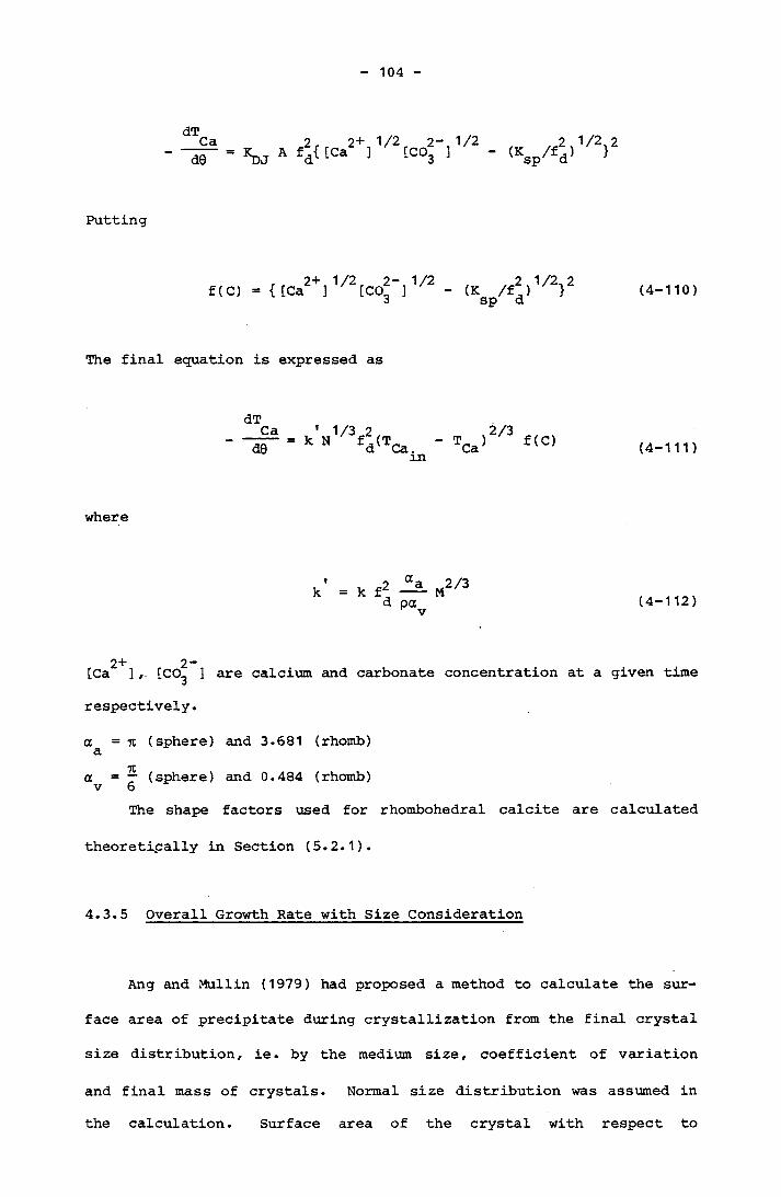
104
d0 V * 4aCa2+]V2[Cof]1/2 - (Ksp/f2d)1/2>2
Putting
f(C) = { [Ca ] 1/2CC0|"]1/2 - (K /f2,1/2}2 3 sp d (4-110)
The final equation is expressed as
dTCad0
' 1/3 2 k N fd(TCa T _ ) Ca
2/3 f (C) (4-111)
where
k k f2 .2/3d pa (4-112)
[Ca ], [CO^ ] are calcium and carbonate concentration at a given time
respectively.
a = n (sphere) and 3.681 (rhomb)3.
71a = — (sphere) and 0.484 (rhomb) v 6The shape factors used for rhombohedral calcite are calculated
theoretically in Section (5.2.1).
4.3.5 Overall Growth Rate with Size Consideration
Ang and Mullin (1979) had proposed a method to calculate the sur
face area of precipitate during crystallization from the final crystal
size distribution, ie. by the medium size, coefficient of variation
and final mass of crystals. Normal size distribution was assumed in
the calculation. Surface area of the crystal with respect to
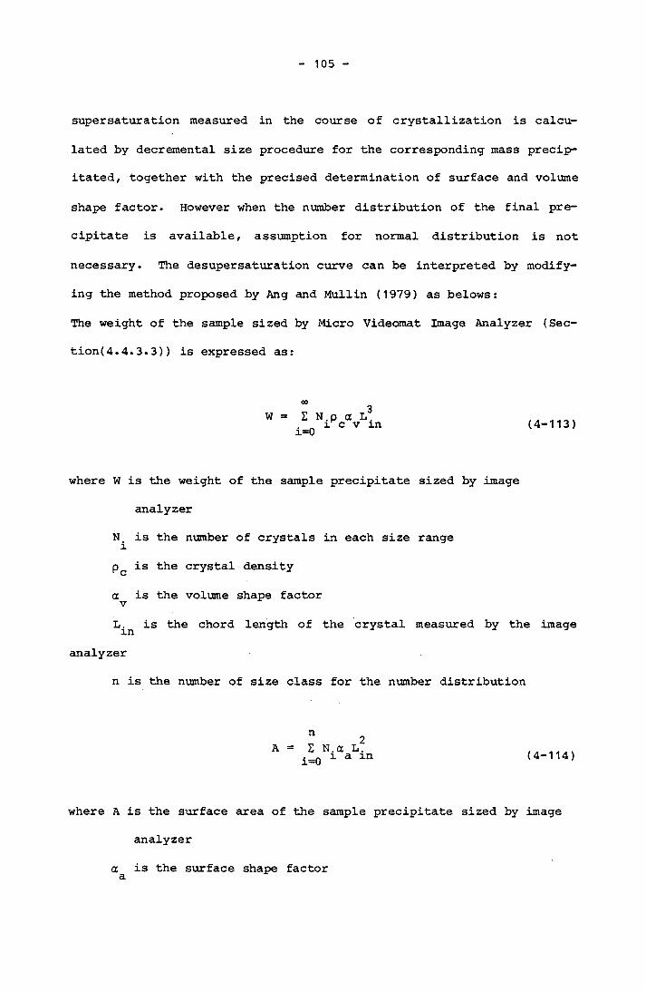
105
supersaturation measured in the course of crystallization is calcu
lated by decremental size procedure for the corresponding mass precip
itated, together with the precised determination of surface and volume
shape factor. However when the number distribution of the final pre
cipitate is available, assumption for normal distribution is not
necessary. The desupersaturation curve can be interpreted by modify
ing the method proposed by Ang and Mullin (1979) as belows:
The weight of the sample sized by Micro Videomat Image Analyzer (Sec-
tion(4.4.3.3)) is expressed as:
W = E N.p a L3 i c v ini=0 (4-113)
where W is the weight of the sample precipitate sized by image
analyzer
N is the number of crystals in each size range ipc is the crystal density
a is the volume shape factor vis the chord length of the crystal measured by the image
analyzer
n is the number of size class for the number distribution
AnE N. a 2L.a in (4-114)
where A is the surface area of the sample precipitate sized by image
analyzer
a is the surface shape factorcL
106
The summation of weight calculated from Equation (4-113) can be
compared with the total weight of the final precipitate, consequently
a weight factor can be calculated by dividing the total weight with
the sample weight. The total surface area of the precipitate is sim
ply the sample surface area multiplied by this factor. The size of
each class of the final precipitate can then be reduced by a small
quantity and the summation of weight and surface area over the entire
size range can be calculated again. The total decremental weight of
the precipitate can be compared with the weight calculated from the
desupersaturation curve. Hence the surface area of the crystal with
respect to time and degree of supersaturation can be calculated. The
process can be repeated to cover a wide range of the desupersaturation curve. By substituting the corresponding values of surface area and
supersaturation into Equation (4-48), the overall growth rate constant
can be calculated. A programme was developed to calcuate the total
weight and surface area of the precipitate for each decremental size
reduction. This can be found in Appendix F (PROG-SIZE).
4.4 EXPERIMENTAL
4.4.1 Introduction
Calcium carbonate crystallization was investigated under bulk
crystallization condition in a batch stirred reactor at constant temperature. Spontaneous crystallization (bulk crystallization without
crystal seeds) was the mode of crystallization for all studies. This
allowed nucleation and crystallization of calcium carbonate to be stu
died in a single experiment. The unseeded crystallization experiments
were also the better representation of the precipitation in the

107
cooling water system. Experiments were carried out at four different
temperatures, viz. 25°C, 36°C, 44°C and 55.8°C. Two geometries for
stirred reactor, viz. Geometry A and Geometry B in conjunction with
different stirring speed were used to study the effect of different
power input to crystal growth rate of calcium carbonate. A wide range
of initial degrees of supersaturation for spontaneous crystallization
was investigated to study its effect on the crystal growth rate con
stants. Apart from crystallization of calcium carbonate in a pure
calcium system, the presence of magnesium equal to calcium molar con
centration was also studied. In a batch crystalization experiment,
the degrees of supersaturation was recorded continually by registering
the pH values of the solution, which could be converted into degree of
supersaturation using programme PROG-CS (see Appendix F). A desuper
saturation curve was constructed for each batch experiment and interpreted for crystal growth rate. Numbers of crystal were counted under
a microscope at the end of each experiment, which was run for at least
four hours. The information about crystal number was required for
crystal growth rate calculation as described in Section (4.3.4). Some
crystal products were sized and photomicrographs were taken. The
scanning electron microscope was also employed to provide detailed
crystals morphology (Appendix B).
4.4.2 Equipment
The major equipment used in the crystallization experiment is a
stirred reactor made of perspex. The detail of the experimental set
up is shown in Figures (4-2) to (4-4). Two geometries, viz. Geometry
A and Geometry B were used in the studies to provide a range of dif
ferent stirring conditions. The individual equipment used is
108
described as follows (Figure (4-2)):(1) Stirred Reactor
This is a 190 mm I.D. diameter cylindrical vessel made of perspex
glass. It comprises one six-bladed brass turbine stirrer with a
stainless steel rod. The stirrer was painted with epoxy paint to
prevent any form of brass corrosion. It was positioned at 1 /o of the
vessel diameter from the base. Four baffles of the width 1/10 vessel
diameter in Geometry A and 1/12 vessel diameter in Geometry B were
installed. The baffles were used to prevent swirling of the solution
and hence achieve even mixing. The vessel was enclosed with a lid
made of perspex. This lid contains openings for pH and temperature
probes. There are also two adaptors to receive the cylindrical tap
funnels by which the reagents are introduced into the reactor. The
joints were sealed with silicone grease. The silicone sealent was used to seal the joints of pH and temperature probes on the lid. Such
arrangement allowed easy removal of the probes for calibration and cleaning. The bearing used for the stirrer rod was a sealed bearing
further secured by a O-ring (Figure (4-3)). Another O-ring was placed
in the circular groove on the flange of the reactor. When the reactor
was closed by putting the lid in position and tightened by the nuts
and bolts, the stirred reactor was completely air-tight. Subsequently
the reactor was immersed in a constant temperature water bath.
(2) Constant Temperature Water Bath
A constant temperature water bath was set up with a Julabo P water
circulator of ±0.02°C accuracy. This provided the necessary tempera
ture control of the solution in the reactor throughout the crystalli
zation experiment.
(3) Resistance Thermometer
Temperature of the solution in the stirred reactor was measured
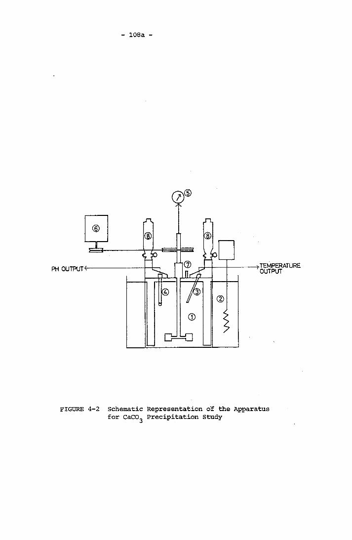
108a
a TEMPERATURE OUTPUTPH OUTPUT <-
FIGURE 4-2 Schematic Representation of the Apparatus for CaCO^ Precipitation Study
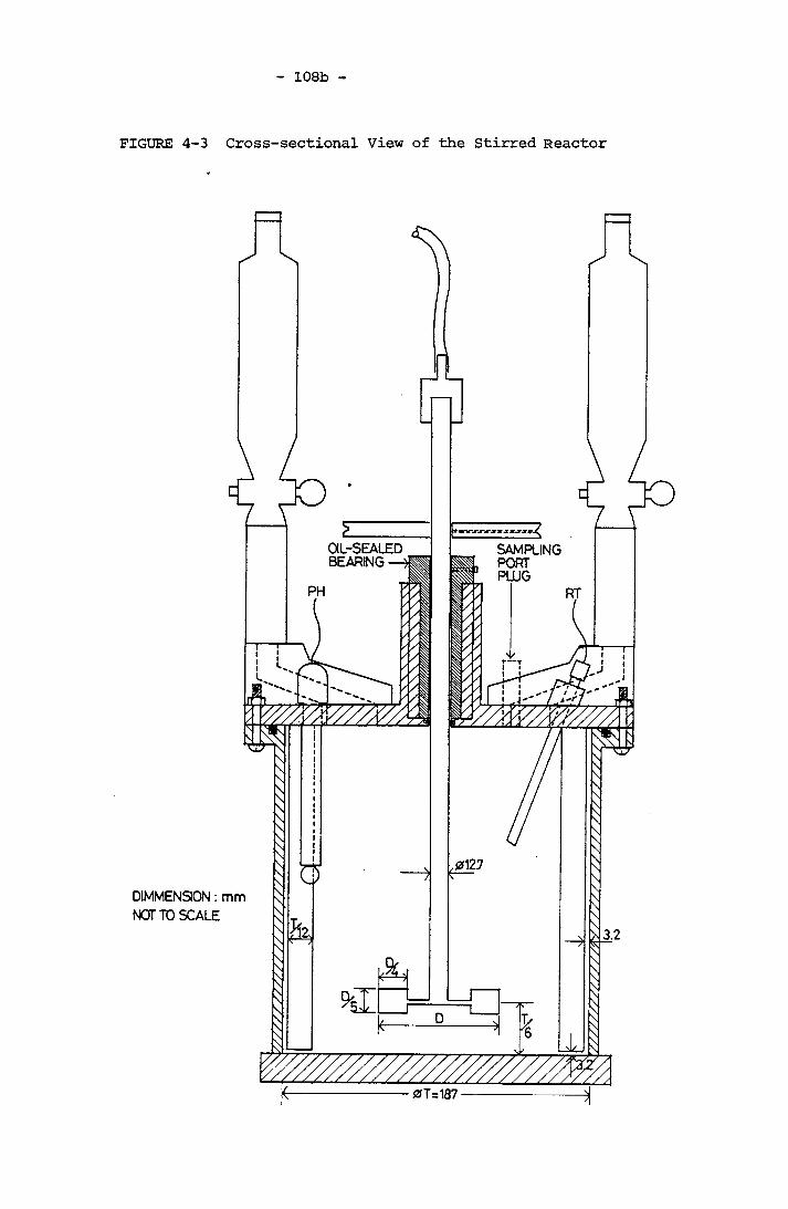
108b
FIGURE 4-3
DIMMENSION :
NOT TO SCALE
Cross-sectional View of the Stirred Reactor
OIL-SEALED BEARING —
SAMPLINGPORTPLUG
0 T=187

108c
FIGURE 4-4 Schematic Representation of Geometry A and Geometry B
T=187
GEOMETRY
]_2
0=62.3
T=187
GEOMETRY B
D_ _ 1 T ‘3
C. 1 T ’ 6
C_ 1 D " 2
D1MMENS10N : mm NOT TO SCALE
109
separately by a 3 wire Pt100 resistance thermometer (Richard Foot Pty.
Ltd., Australia) with ±0.1°C accuracy. The temperature was indicated
by a digital display temperature indicator.
(4) pH Probe and Meter
The pH measurement was conducted by a combination pH probe and
registered by 1852 TPS digital pH meter with readout to the second
decimal point.
(5) Tachometer
The speed of revolution was registered by connecting a flexible tubing
between the stirring rod and the tachometer (Type M.B., Everett
Edgcumbe, England) which generated current in the form of analog read
out in revolutions per minute.
(6) Motor
A fixed rate motor (Parvalux Electric Motors Ltd., Australia) was used
to drive the stirrer at the required speed achieved by different com
bination of pulley size on the motor shaft and on the stirrer rod.
The pulleys were fabricated out of perspex glass. A 1/4 in. nominal
section with 10 in. nominal diameter Merco O-ring (Bestobell Merco)
was used as the belt. Once the tension was fixed, the speed of revo
lution remained constant throughout the experiment.
(7) Sampling Port
An opening was available on the lid to allow crystals sampling. Dur
ing the process of crystallization, this opening was closed tightly by
a plug.
(8) Funnels
Two 100 ml cylindrical tap funnels were placed in the adaptors of the
lid. The calcium chloride and sodium bicarbonate reagents were intro
duced into the reactor simultaneously via these two funnels. Once the
addition process was completed, these funnels remained closed
110
throughout the experiment.
4.4.3 Procedures
4.4.3.1 Batch Stirred Reactor Crystallization Experiments
Distilled water filtered through 0.22|im Millipore membrane filter
was used for all the experiments. All glasswares and the stirred
reactor were thoroughly washed by the following procedure:
The stirred reactor was soaked in 1N hydrochloric acid over night
to remove all the calcium carbonate residue. Subsequently the reactor
together with all the glassware were soaked in 40 °C washing liquid
made of 2 - 3 g/L of Pyroneg (a surgical detergent) for two hours.
They were subsequently brushed and rinsed with plenty of tap water
followed by distilled water. The washing procedure was to minimize
dust in the solution although complete dust-free solution was impossi
ble. All the chemical reagents used were A-R grade. The saturated
solutU-on of calcium carbonate was prepared by mixing sodium bicar
bonate and calcium chloride in distilled water. The required quantity
of sodium bicarbonate for the respective supersaturation was carefully
weighed out and dissolved in 100 mL filtered distilled water. The
solution was filtered again through 0.22 jam membrane filter. Calcium
chloride solution was prepared volumetrically to 100 mL from standar
dised stock solution. Both solutions were then equilibrated to exper
imental temperature in a constant temperature water bath. 4900 mL of
distilled water was carefully measured and transferred into the
stirred reactor and stirred at the required speed in the enclosed
environment. The temperature of the solution eventually reached
equilibrium with the water bath temperature. The experimental tem
perature of the solution in the stirred reactor was separately meas
ured by the Pt100 resistance thermometer to 0.1°C . A torch light
equipped with 4.8V globe was placed at the back of the stirred reactor
to provide the sight of ’zero' turbidity of the solution. pH of the
distilled water was sometimes adjusted by sodium hydroxide solution to
the required reading for high initial degree of supersaturation
intended. To prepare the crystallization experiment for 1:1 Mg/Ca
molar concentration system, magnesium chloride was weighed out
separately to the required quantity and dissolved into 4900 mL of dis
tilled water in the stirred reactor. Once all these initial prepara
tions were completed, solutions of calcium chloride and sodium bicar
bonate were drained simultaneously through two separate cylindrical
tap funnels. The sampling port was left open during the addition of
the reagents. Once the transfer was completed, two stop watches were
started simultaneously and the taps of the funnels and the sampling
port were closed. pH of the solution was recorded with respect to
time followed on one of the stop watch. The other stop watch was used
to register the time taken for the first appearance of shiny nuclei,
ie. the induction period measured by visual observation. The pH read
ings would continue to decrease once crystallization was evident. The
process was given at least four hours to complete. The solution was
then filtered through a 0.22 |j,m membrance filter. The calcium car
bonate crystals were retained on the filter and washed with 200 mL of
distilled water followed by 200 mL of 70% ethyl alcohol to remove the
last traces of residual solution. These crystals were subsequently
dried in the oven at 70 °C overnight and stored in a dessicator for
further microscopic observation.

112
4.4.3.2 Microscopic Observation and Crystal Number Count
The solution was stirred continuously with the speed which was
able to suspend all crystals. The minimum speed was 300 r.p.m. of
Geometry B. This is vital to ensure a uniform sample. A 20 |iL sample
of crystals suspension was taken from the sampling port by a Gilson
micropipette. The sample was then transferred onto the surface of a
counting chamber. The counting chamber has a depth of 0.22 mm and a2total counting area of 9 mm . A cover slip was placed onto the count
ing chamber carefully to spread the crystal suspension evenly over the
counting surface. The 20 size was chosen because it wetted the
entire covered area. Care was taken to spread the crystals over the
entire covered area as evenly as possible, nevertheless the crystals
tend to spread evenly over the counting area which was about 90% of
the entire covered area. Therefore the crystal number is considered
to be slightly higher than the actual number. This error is compen
sated by the possible aging effect of the crystal product by the end
of the experiment. (Section (5.1.5)).
The crystals were examined and counted under 10X objective. For
detail examination the 40X objective was used. The number of crystals
within the counting area was counted and converted to number of cry
stal per litre solution. For each batch experiment, sufficient number
of samples were taken and counted under the microscope to achieve a2statistical significance tested by the x test. The mean was used to
calculate the overall growth rate constant of the bulk crystallization
of calcium carbonate.
113
4.4.3.3 Crystal Size Measurement
Some dried crystal samples were sized to enable overall growth
rate constant determination by size consideration. The crystal sam
ples inevitably contained agglomerates. These agglomerates can be
redispersed in 0.2% sodium pyrophosphate solution. A small quantity
of dried crystal sample was transferred into an approximatley 0.5 mL
of 0.2% sodium pyrophosphate. This crystal suspension was placed in a
ultra-sonic bath generated by a Labsonic 1510 ultra-sound generating
unit at the power input of 10 watts for one minute. This range of
power and duration was found to be suitable to disperse most of the
agglomerates. A drop of this well dispered crystal suspension was
transferred by Pasteur pipette onto a microscope slide. Another drop
of glycerine was added onto the previous drop and subsequently covered
by a cover slip. Glycerine formed the periphery and prevented eva
poration during crystal counting. Crystals were than sized by Micro
videomat 2 in the School of Mining Engineering (Zeiss, 1978, 1980).
This is a instrument with precision television scanning system, often
described as image analyzer. The instrument is comprised of a mono
chrome camera, display, control panel and central processor. Input
comes from a Zeiss Universal microscope fitted with Interference Mono
chromometer for contrast enhancement and transmitted light optics with
highly planar characteristics for flat field coverage. The TV lines
scan the display image from the microscope aerial image. The operator
sets the discriminating level manually. When brightness intensity
deviates from the selected level, a square wave pulse is produced.
The length of scan line within the discriminated image is proportional
to the time parameter on the square wave. The discriminated signal
pulse selected from the continuous background oscillator pulse is
114
further processed, if required, before proceeding to the digital out
put stage. Horizontal TV scan lines and vertical pulses produce 5 6between 10 and 10 picture points scanned in 40 milliseconds. The
control panel may be operated either manually or via HP 9825A computer
keyboard and software. Multiple fields are controlled from the calcu
lator via stepping motors operating in 10 micrometer units. Crystal
numbers as high as 60,000 were scanned and the size was registered as
the TV lines scanned from left to right of the screen. The data input
was presented as first moment distribution (Appendix D).
4.5 RESULTS
4.5.1 Primary Nucleation of Calcium Carbonate Precipitation
4.5. 1.1 Experiments at Constant Stirring Speed
A series of experiments were conducted on the stirred reactor
with Geometry A as described in Section (4.4.2) for the crystalliza
tion studies. The induction periods were determined by visual obser
vation at different temperatures over a wide range of initial degrees
of supersaturation. The degree of supersaturation throughout this2+ 2- 2 [Ca ] [C03 ] fd
project is defined as S = ----- ---------. The time taken for theK.sp
first appearance of shiny crystals was registered as induction period
(0. ). The latent period (9 ) was also registered as the timemd lattaken for the first detection of pH decrease from the maximum pH value
created after mixing. The stirring speed was 220±5 r.p.m. The total
volume of the solution in the reactor was 5.1 litre. The results are
tabulated in Tables (4-2) and (4-3).
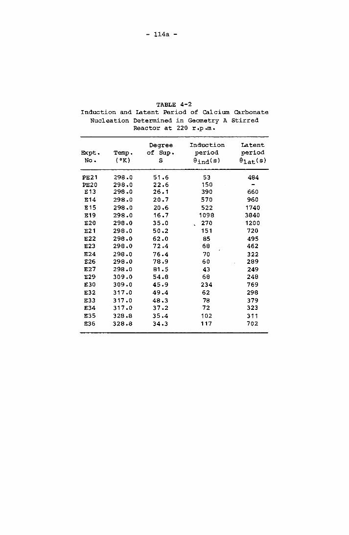
114a
TABLE 4-2Induction and
NucleationLatent PeriodDetermined in Reactor at 220
of CalciumGeometry Ar .p .m.
CarbonateStirred
Degree Induction LatentExpt. Temp. of Sup. period periodNo . (°K) S 9ind(s) eiat(s)
PE21 298.0 51 .6 53 484PE20 298.0 22.6 150 -
E 13 298.0 26.1 390 660E14 298.0 20.7 570 960E 1 5 298.0 20 .6 522 1740E19 298.0 16.7 1098 3840E20 298.0 35.0 . 270 1200E21 298.0 50 .2 151 720E22 298.0 62.0 85 495E23 298.0 72.4 68 462E24 298.0 76.4 70 322E26 298.0 78.9 60 289E27 298.0 81 .5 43 249E29 309.0 54.8 68 248E30 309.0 45.9 234 769E32 317.0 49.4 62 298E33 317.0 48.3 78 379E34 317.0 37.2 72 323E35 328 .8 35.4 102 311E36 328.8 34.3 117 702
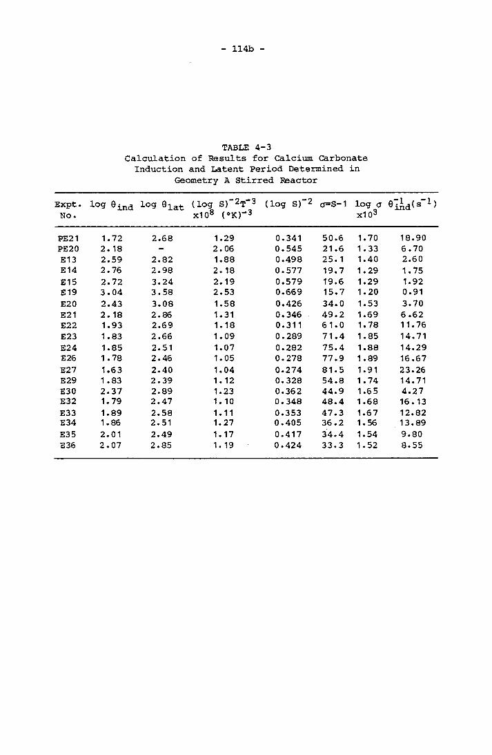
114b
TABLE 4-3Calculation of Results for Calcium Carbonate Induction and Latent Period Determined in
Geometry A Stirred Reactor
Expt. No. lo9 9ind lo9 9lat (log S)"2T”3
x108 (°K)-3(log S)"2 cr=S-1 log a
x1 03 Sind'3'1)
PE2 1 1.72 2.68 1.29 0.341 50.6 1.70 18.90PE20 2.18 - 2.06 0.545 21.6 1.33 6.70E13 2.59 2.82 1.88 0.498 25. 1 1.40 2.60E14 2.76 2.98 2. 18 0.577 19.7 1.29 1.75E15 2.72 3.24 2.19 0.579 19.6 1.29 1.92E 19 3.04 3.58 2.53 0.669 15.7 1.20 0.91E20 2.43 3.08 1.58 0.426 34.0 1.53 3.70E21 2. 18 2.86 1.31 0.346 49.2 1.69 6 .62E22 1.93 2.69 1.18 0.311 61.0 1.78 11.76E23 1.83 2.66 1.09 0.289 71.4 1.85 14.71E24 1.85 2.51 1.07 0.282 75.4 1.88 14.29E26 1.78 2.46 1.05 0.278 77.9 1.89 16.67E27 1.63 2.40 1.04 0.274 81.5 1.91 23.26E29 1.83 2.39 1. 12 0.328 54.8 1.74 14.71E30 2.37 2.89 1.23 0.362 44.9 1.65 4.27E32 1.79 2.47 1. 10 0.348 48.4 1 .68 16.13E33 1.89 2.58 1.11 0.353 47.3 1.67 12.82E34 1.86 2.51 1.27 0.405 36.2 1.56 13.89E35 2.01 2.49 1.17 0.417 34.4 1.54 9.80E36 2.07 2.85 1. 19 0.424 33.3 1.52 8.55

115
4.5. 1.2 Experiments at Different Stirring Speed
A series of experiments were conducted at 300, 400, 500, 700 and
880 r.p.m. using Geometry B at 25°C. The results are tabulated in
Tables (4-4) and (4-5).
4.5. 1.3 Experiments at Different Stirring Speed of _1_:_1_ Mg/Ca Molar
Concentration
The presence of magnesium cations is known to retard the rate of
nucleation and crystallization of calcium carbonate. In this experi
ment the effect of stirring was investigated at 1:1 Mg/Ca molar ratio
at 25°C under similar supersaturation condition. Geometry B stirred
reactor was used for this series of experiments. The results are
tabulated in Table (4-6) for both induction period and latent period.
4.5.2 Secondary Nucleation of Calcium Carbonate Precipitation
Secondary nucleation is heterogeneous nucleation and occurs due
to the collision of crystals against other crystals and the collision
of crystals against other objects. Therefore, it is not unreasonable
to expect secondary nucleation in a stirred reactor as used in these
experiments. In fact this mode of nucleation is considered to be the
major source of new crystals in a industrial crystallizer when stirr
ers and pumps are used to move the crystals suspension in the crystal
lizer (Bennett, et. al., 1973). In a batch reactor crystallization
process, nucleation takes place after the precipitating solutions are
mixed together. This continues for a period of time until crystalli
zation predominates, which is indicated by a significant decline of

115a
TABLE 4-4Induction and Latent Period of Calcium Carbonate Nucleation in Geometry B Reactor at 25°C under Different Stirring Speed and Supersaturation
Expt.No.
Degree of Sup.
S
InductionPeriod9ind
LatentPeriodelat (s)
Stirring Speed
(r.p.m.)
PE5 57.0 126 920 500PE 7 58.0 120 751 500PE 11 25.6 174 3518 500PE 14 39.3 96 2757 500PE 16 76.5 39 303 500PE 8 57.0 84 724 400PE 9 57.0 192 1083 400PE13 25.6 174 10560 400PE6 62.8 162 1066 300PE 3 59.0 96 948 300PE 15 57.0 84 324 700PE 4 57.0 156 96 5 880PE 12 35.6 132 16020-16440 880
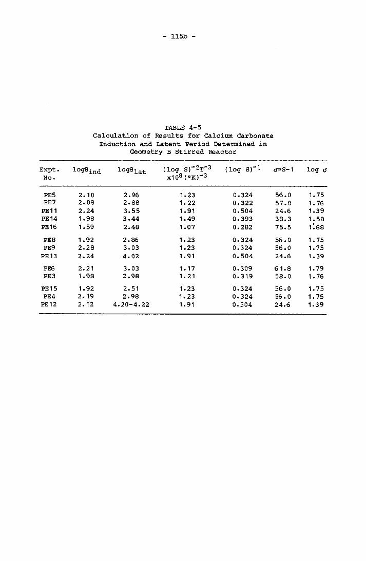
115b
TABLE 4-5Calculation of Results for Calcium Carbonate Induction and Latent Period Determined in
Geometry B Stirred Reactor
Expt. No. lo9Sind lo9®lat (log S)"2T"3
x108(°K)"3(log S)_1 a=S-1 log a
PE 5 2.10 2.96 1.23 0.324 56.0 1.75PE7 2.08 2.88 1.22 0.322 57.0 1.76PE 1 1 2.24 3.55 1.91 0.504 24.6 1.39PE 14 1.98 3.44 1.49 0.393 38.3 1.58PE 16 1.59 2.48 1.07 0.282 75.5 r.88PE 8 1.92 2.86 1.23 0.324 56.0 1.75PE9 2.28 3.03 1.23 0.324 56.0 1.75PE 13 2.24 4.02 1.91 0.504 24.6 1.39PE6 2.21 3.03 1.17 0.309 6 1.8 1.79PE3 1.98 2.98 1.21 0.319 58.0 1.76PE 15 1.92 2.51 1.23 0.324 56.0 1.75PE 4 2.19 2.98 1.23 0.324 56.0 1.75PE 12 2.12 4.20-4.22 1.91 0.504 24.6 1.39

115c
TABLE 4-6Induction and Latent Period of Calcium Carbonate
Nucleation of S=24 determined in Geometry B Reactor with 1=1 Mg/Ca Molar Ratio at 25°C
Expt.InductionPeriod0ind(S)
LatentPeriod9ind(s ^
Stirring Speed
(r.p.m.)
PE 17 128 3552 500PE18 120 2076 700PE 19 219 7218 400
116
measurable properties such as conductivity or pH. During the period
of nucleation, the number of nuclei (miniature crystals) continues to
increase until it reaches a constant number, ie. crystal growth takes
over the process. This constant crystal number corresponds to the
commencement of the steep decline of the desupersaturation curve (see
Figure (4-1)). Assuming secondary nucleation is the major source of
nuclei generated, also assuming constant rate of increase in number of
nuclei over the entire period (this fact was observed and illustratedANin Figure (5-10)), then secondary nucleation is expressed as ~ where
AN is the number of crystals counted at the end of crystallization. A0
is the time taken to reach a constant crystal number.
Ottens et. al. (1972) derived the equation for nucleation due to crystal-stirrer collision as well as crystal-crystal collision (see
Equations (2-24) and (2-25)). The energy dissipitated per unit mass
of slurry in the stirred reactor designed for the present experiment
can be calculated directly. The detailed calculation is described in
the following section.•9
4.5.2.1 The Calculation of Power Input in a Stirred Reactor
The power input from the impeller into the agitated liquid of the stirred reactor can be calculated from the empirical equation derived
by dimensional analysis. The development of the generalized form of an equation for correlating power has been covered by Johnstone and
Thring (1957) and Rushton, et. al. (1950a, 1950b). The general equa
tion is expressed as:
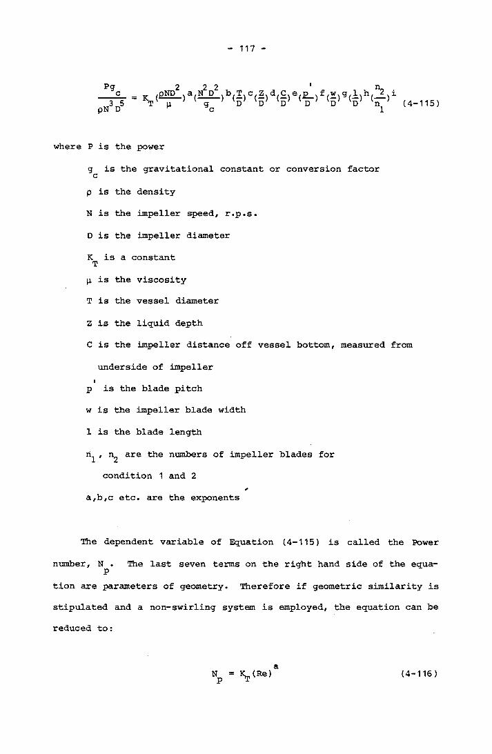
117
Pgc
where P is the power
g is the gravitational constant or conversion factor cp is the density
N is the impeller speed, r.p.s.
D is the impeller diameter
K is a constant Tp, is the viscosityT is the vessel diameter
Z is the liquid depth
C is the impeller distance off vessel bottom, measured from
underside of impellerI
p is the blade pitch
w is the impeller blade width
1 is the blade length
n^ , n^ are the numbers of impeller blades for
condition 1 and 2
a,b,c etc. are the exponents
The dependent variable of Equation (4-115) is called the Power
number, N . The last seven terms on the right hand side of the equa
tion are parameters of geometry. Therefore if geometric similarity is stipulated and a non-swirling system is employed, the equation can be reduced to:
P
aNp - VRe) (4-116)
118
where Re is the first dimensional group of the equation known as Rey
nolds number.
Bates, et. al. (1963) had conducted power input measurement on
specified geometry and reported the Power number against Reynolds
number of Newtonian fluids for various turbine impeller designs. The4Power number is constant when the Reynolds number exceeds 10 for the
radial six-blade turbine impeller. In this research project, the
stirred reactor of Geometry B (see Figure (4-4)) was built according
to the geometry specified by Bates, et. al. (1963) except the postiton
of the impeller was at C/T=1/6. The Geometry A (Figure (4-4)) stirred
reactor adopted 4 baffles with the width w^=T/10 and the turbine
impeller of D/T=1/2 diameter. Such disimilarities in the geometry
incur some modification on the Power number based on the standard
geometry specified by Bates, et. al. The corrections were also given
by Bates et. al. (1963). The resulting Power numbers for Geometry A
and Geometry B are 4.8 and 4.5 respectively. An example of the power
input calculation based on the Power number of the corresponding Rey
nolds number and stirred reactor and impeller geometry is given as
follows: Geometry B stirred reactor
N = 300 r.p.m. = 5 r.p.s.-3D = 62.3 mm = 62.3 x 10 m
-3p, = 0.890 multiply 10 kg/m s at 25°C
p = 997.04 kg/m3 at 25°C2 -3 2Re = D HP = (62.3 x 10 ) x 5 x 997.04^ 0.890 x 10"3
=2.174 x10⁴

119
Therefore N is a constant which is equal to K . K =4.5 p T T
3 5V D p
4.5 x 53 x (62.3 x 10~3)5 x 997.04
0.5264 J/s
Therefore the power input per unit volume, e 0.52645.1 0. 1032 J/L s
4.5.2.2 Experiments of Pure Calcium Carbonate System
The Geometry B reactor was used for the investigation except for one experiment which used Geometry A reactor. The experimental pro
cedure is exactly the same as crystallization experiment described in Section (4.4.3. 1) except the numbers of crystals at the end of the
experiment was counted in the counting chamber under a microscope. In
experiment PE21 samples were taken during the nucleation process and
the crystals number counted. The experiments were conducted at dif
ferent initial degrees of supersaturation and different stirring
speeds. All the experiments were conducted at 25 °C. The data of
desupersaturation curve with respective to time of the bulk crystallization are given in Appendix A and C. The results are summarised and
tabulated in Table (4-7).
4.5.2.3 Experiments on Mg/C a Molar Concentration
Samples were taken during the nucleation process for crystals
count in experiment PE 19 (see Figure (5-13)). The final crystals
counts were carried out for all experiments. The results are
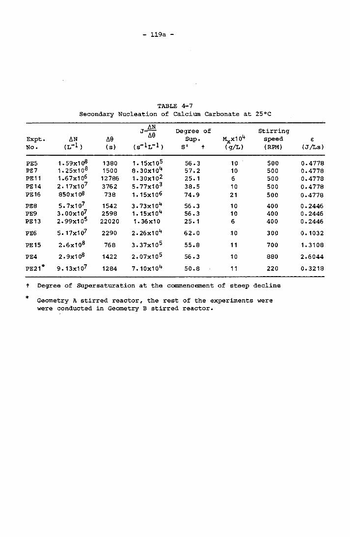
119a
TABLE 4-7Secondary Nucleation of Calcium Carbonate at 25°C
Expt.No .
AN(IT1 )
A9(s)
ANJ_A9
(s^L-1 )
Degree of Sup.
S' +IV^xlO4 (g/L)
Stirringspeed(RPM)
£(J/Ls)
PE5 1.59x1 08 1380 1.15x10⁵ 56.3 10 500 0.4778PE 7 1.25x10⁸ 1500 8.30x10⁴ 57.2 10 500 0.4778PE11 1 .67x1 06 12786 1.30x10² 25. 1 6 500 0.4778PE 14 2.17x10⁷ 3762 5.77x10³ 38.5 10 500 0.4778PE16 850x108 738 1.15x10⁶ 74.9 21 500 0.4778PE 8 5.7x10⁷ 1542 3.73x10⁴ 56.3 10 400 0.2446PE9 3.00x10⁷ 2598 1.15x10⁴ 56.3 10 400 0.2446PE 13 2.99x10⁸ 22020 1.36x10 25. 1 6 400 0.2446PE6 5. 17x1 07 2290 2.26x1 04 62.0 10 300 0. 1032PE 15 2.6x10⁸ 768 3.37x10⁵ 55.8 11 700 1.3108PE4 2.9x10⁸ 1422 2.07x10⁵ 56.3 10 880 2.6044PE21 * 9.13x107 1284 7.10x10⁴ 50.8 11 220 0.3218
t Degree of Supersaturation at the commencement of steep decline•fc Geometry A stirred reactor, the rest of the experiments were
were conducted in Geometry B stirred reactor.
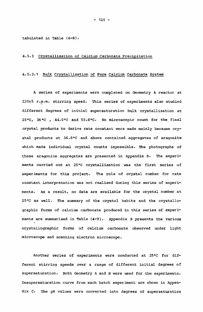
120
tabulated in Table (4-8).
4.5.3 Crystallization of Calcium Carbonate Precipitation
4.5.3.1 Bulk Crystallization of Pure Calcium Carbonate System
A series of experiments were completed on Geometry A reactor at
220±5 r.p.m. stirring speed. This series of experiments also studied
different degrees of initial supersaturation bulk crystallization at
25°C, 36°C / 44.0°C and 55.8°C. No microscopic count for the final
crystal products to derive rate constant were made mainly because cry
stal products at 36.0°C and above contained aggregates of aragonite
which made individual crystal counts impossible. The photographs of
these aragonite aggregates are presented in Appendix B. The experi
ments carried out at 25°C crystallization was the first series of
experiments for this project. The role of crystal number for rate constant interpretation was not realised during this series of experi
ments. As a result, no data are available for the crystal number at
25°C as well. The summary of the crystal habits and the crystallo
graphic forms of calcium carbonate produced in this series of experi
ments are summarised in Table (4-9). Appendix B presents the various
crystallographic forms of calcium carbonate observed under light
microscope and scanning electron microscope.
Another series of experiments were conducted at 25°C for dif
ferent stirring speeds over a range of different initial degrees of
supersaturation. Both Geometry A and B were used for the experiments.
Desupersaturation curve from each batch experiment are shown in Appen
dix C. The pH values were converted into degrees of supersaturation
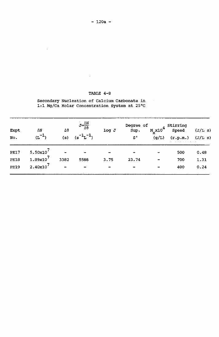
120a
TABLE 4-8Secondary Nucleation of Calcium Carbonate in 1:1 Mg/Ca Molar Concentration System at 25°C
ExptNo.
AN(l"1)
A0(s)
_ ANJ=A0
(s'V1)log J
Degree of StirringSup. M^xlO SpeedS' (g/L) (r.p.m.)
(J/L s)(J/L s)
PE17 5.50xl07 - - - 500 0.48PE18 1.89xl07 3382 5588 3.75 23.74 - 700 1.31PE19 2.40xl07 - - - 400 0.24
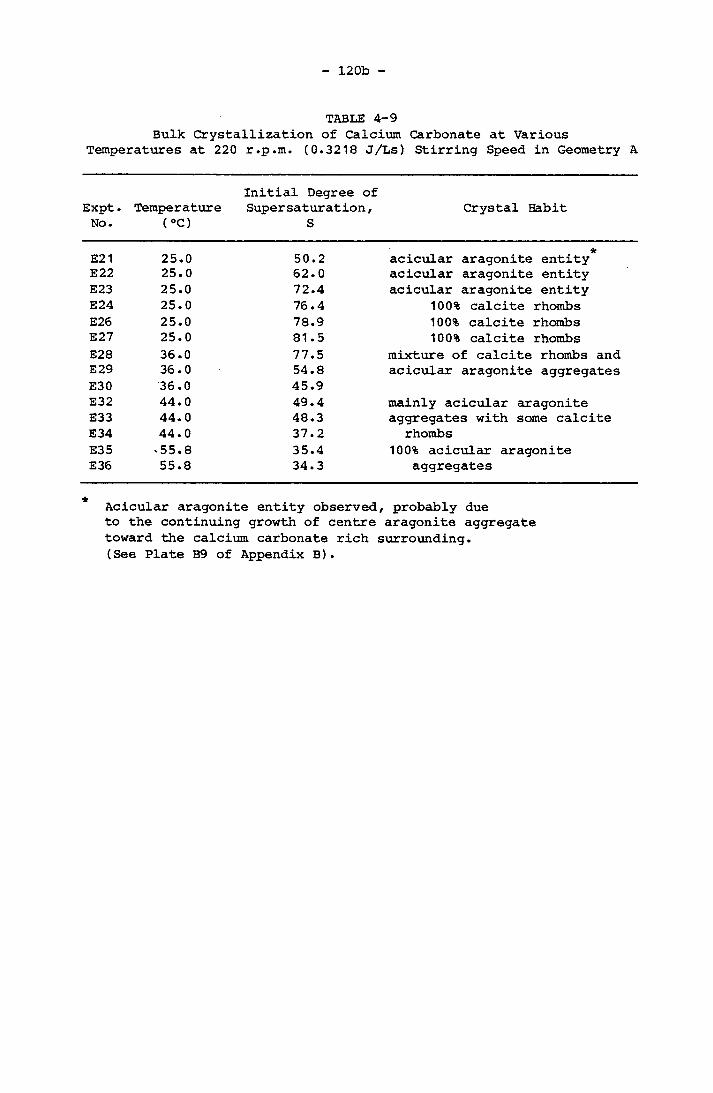
120b
TABLE 4-9Bulk Crystallization of Calcium Carbonate at Various
Temperatures at 220 r.p.m. (0.3218 J/Ls) Stirring Speed in Geometry A
Initial Degree ofExpt. Temperature Supersaturation, Crystal HabitNo. (°C) S
E21 25.0 50.2E22 25.0 62.0E23 25.0 72.4E24 25.0 76.4E26 25.0 78.9E27 25.0 81.5E28 36.0 77.5E29 36.0 54.8E30 36.0 45.9E32 44.0 49.4E33 44.0 48.3E34 44.0 37.2E35 *55.8 35.4E36 55.8 34.3
*acicular aragonite entity acicular aragonite entity acicular aragonite entity
100% calcite rhombs 100% calcite rhombs 100% calcite rhombs
mixture of calcite rhombs and acicular aragonite aggregates
mainly acicular aragonite aggregates with some calcite
rhombs100% acicular aragonite
aggregates
Acicular aragonite entity observed, probably due to the continuing growth of centre aragonite aggregate toward the calcium carbonate rich surrounding.(See Plate B9 of Appendix B).
121
as well as the content of calcium with respective to time by the pro
gramme PROG-CS. The data and results are available in Appendix A and
C. The final crystal number was counted in the counting chamber under
the microscope. The final crystals of some experiments were sized by
Micro-videomat 2 and the results are given Appendix D. The overall
growth rate constant was calculated for each batch experiment accord
ing to Sections (4.3.4) and (4.3.5). The results are summarised in
Tables (4-10) and (4-11). The values of dT /d0 can be obtained from
the desupersaturation curve of T^ against time. A best straight line2/3can be drawn through the plot of dT /d0/(T -T ) againstCa Ca. Cain
2+ 1/2 2- 1/2 2 1/2 2{[Ca ] [CCL ] -(K /f,) } for the overall growth rate constant3 sp ddetermined by simplified method and dT^/d0/A against
2+1/2 2~1/2 21/22{[Ca ] [CCL ] -(K /f,) } for the overall growth rate constant3 sp ddetermined by surface area calculated based on size distribution. The
plots for all the experiments are shown in Appendix C. The gradient• 1 /3of the former is therefore equal to k N . The overall growth rate
constant k for bulk crystallization can be calculated from Equationt f
(4-111). The gradient of the latter is therefore equal to k and the overall growth rate constant k can be calculated from Equation (4-48).
Some of the photomicrographs of the crystal samples are available in
Appendix B. All the three crystallographic forms of calcium car
bonate, namely calcite, aragonite and vaterite were observed. The
calcite is in rhomohedral crystal habit. The aragonite is an aggre
gate of acicular crystals. The vaterite appears in the form of spherical crystals. The aragonite crystals were also observed in the
unique crystal habit which probably was the result of the continuing
growth of the bundle of acicular aragonite crystals. A typical ara
gonite entity is shown, in Plate 9 of Appendix B.
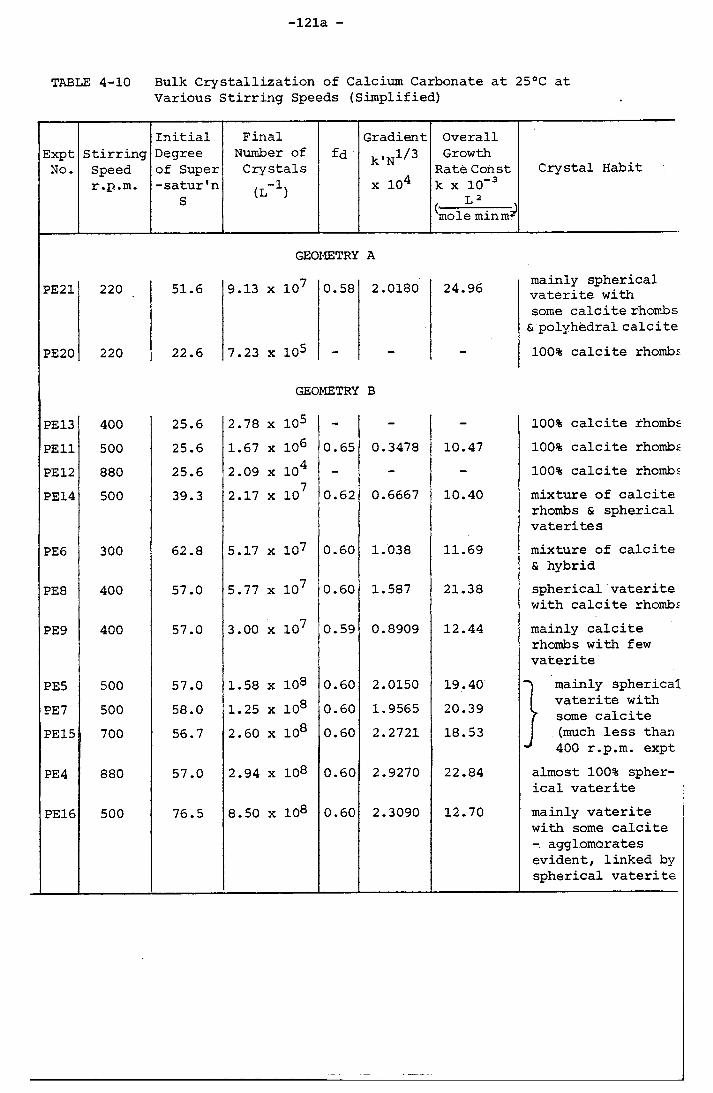
-121a
TABLE 4-10 Bulk Crystallization of Calcium Carbonate at 25°C at Various Stirring Speeds (Simplified)
ExptNo.
StirringSpeedr.p.m.
Initial Degree of Super -satur'n
S
FinalNumber of Crystals(L_1)
fdGradientk'N1/3 x 10* * * 4
OverallGrowth
Rate Const k x 10"3( L2 J'"mole minm2'
GEOMETRY A
PE21 220 51.6 9.13 x 10⁷ 0.58 2.0180 24.96
PE20 220 22.6 7.23 x 10⁵ - - -
GEOMETRY B
PE 13 400 25.6 2.78 x 10⁵ - - -PE 11 500 25.6 1.67 x 10⁶ 0.65 0.3478 10.47PE12 880 25.6 2.09 x 10⁴ - - -PE14 500 39.3 2.17 x 10⁷ 0.62 0.6667 10.40
PE 6 300 62.8 5.17 x 10⁷ 0.60 1.038 11.69
PE8 400 57.0 5.77 x 10⁷ 0.60 1.587 21.38
PE9 400 57.0 3.00 x 10⁷ 0.59 0.8909 12.44
PE5 500 57.0 1.58 x 10⁸ 0.60 2.0150 19.40PE 7 500 58.0 1.25 x 10⁸ 0.60 1.9565 20.39PE15 700 56.7 2.60 x 10⁸ 0.60 2.2721 18.53
PE 4 880 57.0 2.94 x 10⁸ 0.60 2.9270 22.84
PE16 500 76.5 8.50 x 10⁸ 0.60 2.3090 12.70
Crystal Habit
mainly spherical vaterite with some calcite rhombs & polyhedral calcite100% calcite rhombs
100% calcite rhombs100% calcite rhombs100% calcite rhombsmixture of calcite rhombs & spherical vateritesmixture of calcite& hybridspherical vaterite with calcite rhombsmainly calcite rhombs with few vaterite
mainly spherical vaterite with some calcite (much less than 400 r.p.m. expt
almost 100% spherical vateritemainly vaterite with some calcite - agglomerates evident, linked by spherical vaterite
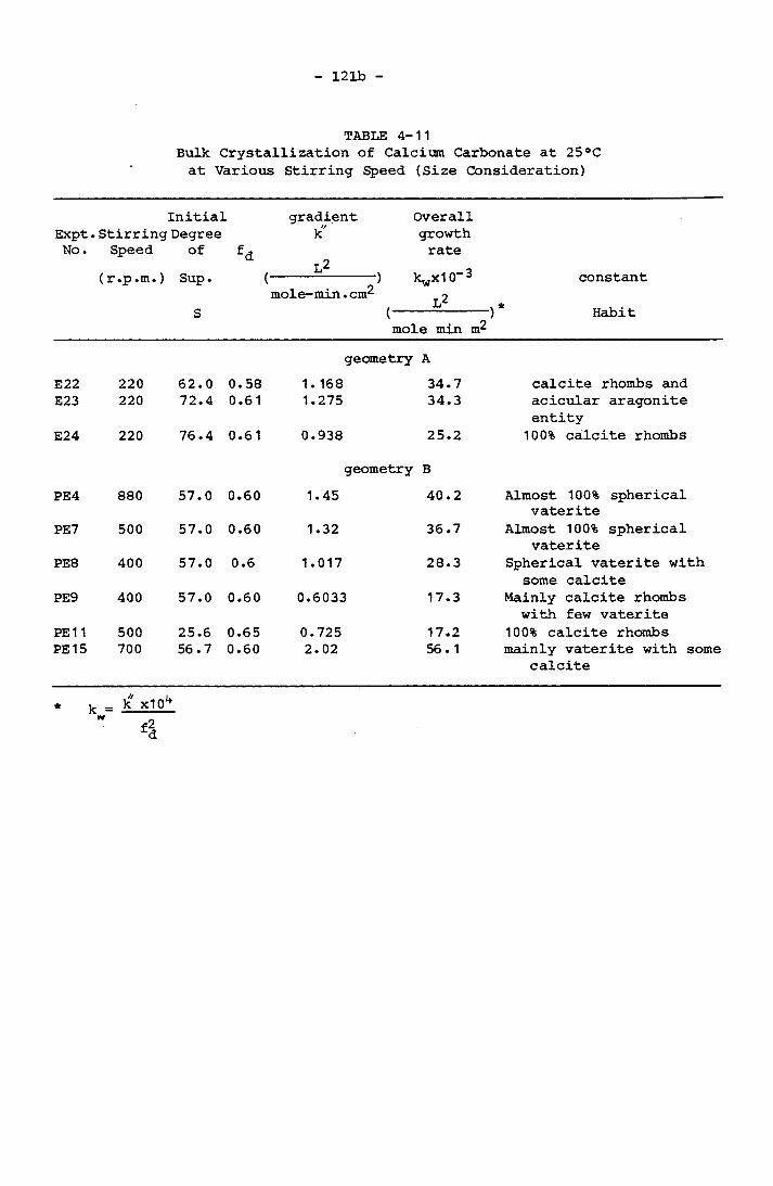
121b
TABLE 4-11Bulk Crystallization of Calcium Carbonate at 25°Cat Various Stirring Speed (Size Consideration)
Initial gradient OverallExpt. Stirring Degree k" growthNo. Speed of fd _ 9
rate(r.p.m. ) Sup. ( ) kwx10”3 constant
mole- min. cm^ T 2S ( —----- > Habit
mole min m^geometry A
E22 220 62.0 0.58 1. 168 34.7 calcite rhombs andE23 220 72.4 0.61 1.275 34.3 acicular aragonite
entityE24 220 76.4 0.61 0.938 25.2 100% calcite rhombs
geometry BPE4 880 57.0 0.60 1.45 40.2 Almost 100% spherical
vateritePE 7 500 57.0 0.60 1.32 36.7 Almost 100% spherical
vateritePE 8 400 57.0 0.6 1.017 28.3 Spherical vaterite with
some calcitePE 9 400 57.0 0.60 0.6033 17.3 Mainly calcite rhombs
with few vateritePE1 1 500 25.6 0.65 0.725 17.2 100% calcite rhombsPE 15 700 56.7 0.60 2.02 56.1 mainly vaterite with some
calcite
* k = ^ xIO1*
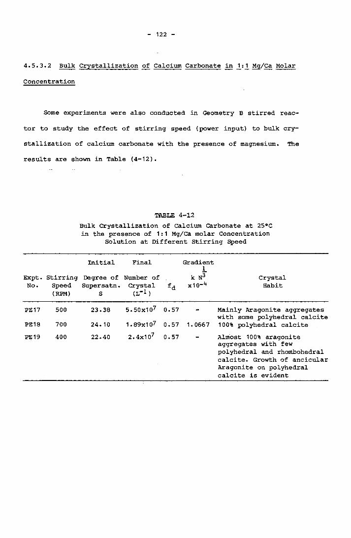
122
4.5.3.2 Bulk Crystallization of Calcium Carbonate in Mg/Ca Molar
Concentration
Some experiments were also conducted in Geometry B stirred reac
tor to study the effect of stirring speed (power input) to bulk cry
stallization of calcium carbonate with the presence of magnesium. The
results are shown in Table (4-12).
TABLE 4-12Bulk Crystallization of Calcium Carbonate at 25°C in the presence of 1:1 Mg/Ca molar Concentration
Solution at Different Stirring Speed
Initial Final Gradient1Expt. Stirring Degree of Number of k N3 CrystalNo. Speed Supersatn. Crystal fd x10-4 Habit
(RPM) S (L"1 )
PE 17 500 23.38 5.50x1071.89x107
0.57 - Mainly Aragonite aggregates with some polyhedral calcite
PE 18 700 24. 10 0.57 1.0667 100% polyhedral calcitePE 19 400 22.40 2.4x10⁷ 0.57 Almost 100% aragonite
aggregates with few polyhedral and rhombohedral calcite. Growth of ancicular Aragonite on polyhedral calcite is evident
123
CHAPTER 5
DISCUSSION OF CALCIUM CARBONATE PRECIPITATION STUDIES
5.1 NUCLEATION OF CALCIUM CARBONATE
5.1.1 General
The study of nucleation of calcium carbonate has adopted the
approach of induction period. Induction period can be related to the
classical nucleation period to calculate other importat information
such as interfacial energy, critical nucleus size and 'order' of nucleation.
5.1.2 Visual Induction Period Data
In Figure (5-1), the induction periods measured from experiments
conducted under constant and different speed of mixing are readily
grouped into two regions. The boundary of these two regions is indi-— 2 —3 —8 —2 —3 —8cated by (log S) T at 1.23x10 °K. For (log S) T > 1.23x10 ,
line B can be constructed. Line B passes through points obtained from
experiments at 200 r.p.m. stirring speed that produced mixture of cal-
cite and aragonite (Section (4.5.3.1)). This region clearly shows the
effect of heterogeneous nucleation which reduces the induction period
and is expected at lower initial degrees of supersaturation. Parti
cles of diameter less than 1 |im cannot be observed easily in an
intense beam of light. Hence for low particle concentrations it is
very difficult to observe the nucleus sized particles. The problems
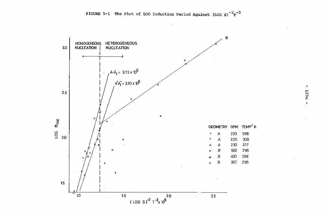
HOMOGENEOUS HETEROGENEOUS NUCLEATION I NUCLEATION
123a
iCNI3■Ptfla•H(dO'<T5O•HU<DCU•H+JO3T3CMO34-J
OCOincvi
Ocsi
pu|0
901
( LOG S )'
124
are compunded by the presence of heteronuclei in solutions of lower
degrees of supersaturation. Hence data on heterogeneous nucleation
are considered to be less reliable and subject to greater error than
for other experimental conditions. The effect of stirring speed
(power input) is not certain especially because heteronuclei have a
strong influence in this region. However, lines A and A' have a
steeper gradient than lines B and B'. These points were obtained from
stirred reactor experiments with higher degrees of supersaturation.
The gradient of the straight line is the result of homogeneous nuclea
tion of calcium carbonate.
Sohnel and Mullin (1982) used Nielsen's (1967, 1969) approach to
assume homogeneous nucleation, followed by diffusional growth of the
created nuclei. The induction period of precipitation may be con
sidered to obey the Equations (4-3) and (4-4) (Section (4.1.2)). The
derivation of these equations was given in the papers published by
Nielsen (1964, 1967, 1969, 1971). The diffusional growth of the
created nuclei to the size that is either visible or causes changes of
a ipeasurable property is considered a valid assumption. Crystals less
than 10 |i,m have relatively slow velocity through the solution in a
normal gravity field or at normal stirring rates, ie. for submicros-
copic crystal growth, convection can be neglected (Nielsen, 1964;
Konak, 1971). In some experiments, samples of solution at the initial
stage of crystallization were observed under the microscope and the
nuclei (closely resembling a spherical shape) were as small as 1 p,m.
It is well known that bacteria (which are approximately 1 |im in size)
in large populations can be detected visually as turbidity in solu
tion. Therefore, the induction period measured by visual observation
is an indication of the presence of nuclei (miniature crystals) of at
125
least 1 (j.m size but the nuclei are still small enough to be considered
due to diffusion controlled growth. The characteristic time or time
scale (0^) is expressed in the following equation (Nielsen and Sohnel,
1971 ) :
c. - cin_____c. - c m s
J^d2/3iv (c. - c >]1/2ef/215 m in s 1 (5-1 )
where is some arbitrary constant characteristic of the degree of
precipitation when diffusion-controlled growth is still
validI
c is an arbitrary concentration to establish a characteristic
constant
c. is the initial concentration in
When c is increased, Q decreases so 0 decreases to reach a in ind 1 1when homogeneous nucleation predominates. 0. , is a significant meas-indure of the time required for nuclei to grow to 1 |im size. Therefore,
0^ is proportional to the induction period within the range of the
diffusion controlled growth mechanism. From Equation (5-1),
Inserting
and
where D is the diffusion coefficient
d is the molecular diameter m
1509i ■ f16W2JD3/2[V (c. - c )]1/2mm s
2/5(5-2)
2D *J = — exp(-AG AT) (Nielsen, 1964)dm*'32 2AG = p a V /(KT In S)

126
Taking logarithm and rearrange Equation (5-2)
15a, d 1 mln0 | — In [ c /o 1 /p
1 16h/2D5/2V1/2(
' 3 2.2/5 2P ° Vm
1 /2J 3 2c. - c ) ,/z 5(KT) (InS) (5-3)m in s
Since 9 is proportional to 9. which is measured experimentally,ind
tanking 9. = 9. .,1 md
log 9ind const. + at/(log S) (5-4)
where
' 3 2 2p a V
5(KTlnl0)(5-5)
-2 -2 -3Therefore, the plot of against (log S) and (log S) T (in
the case of data available from more than one temperature) enables the
calculation of interfacial energy from the gradient of the plot. Fig-
8ure (5-1) gives the value = 3.73x10 "or homogeous nucleation of
calcium carbonate. The straight line passes through data obtained
from calcite nucleation at 25°C and the mixtures of calcite and ara-
' 8gonite from 36°C and 44°C. The value =3.10x10 is obtained from
line A' which passes through data obtained from vaterite nucleation at
025 C. Substituting the following values for calcite:
-23 3 -23 -1(3 = 32 (cube), V = 3.067x10 cm and K = 1.3805x10 J°K ,
3a5K3(ln10)3at
22|3V r m
9.95x10⁻¹⁶ (J/cm2)3
127
a = 101 nvJ/m2
The value of p = --- (sphere) for vaterite
3 --—-- - = 1.58x1028 V2“ m
am
a = 118 nvJ /m2
The value of calcite interfacial energy is similar to values reported
by other workers (Nielsen and Sohnel, 1971; Sohnel and Mullin, 1978;
Kharin et. al., 1980; Sohnel and Mullin, 1982). Although vaterite was
found to possess a slightly higher interfacial energy than calcite/
the lower a (therefore a smaller free energy required for nucleation)
indicates an overall faster nucleation rate than calcite.
The empirical relationship (see Equation (4-49)):
based on the concept of metastable region (Miers and Isaac, 1906) has
frequently been used.
where K is the nucleation rate constant nc is the solute concentration
c is a concentration greater than the saturated concentration mbelow which nucleation does not occur.
In inorganic salt system, c also can be replaced by the saturatedmconcentration c^ without affecting significantly the empirical rela
J=K(c-c)n = K Ac11 n m n (5-6)
tionship (Randolph and Larson, 1971). Therefore by defining a as the
128
supersaturation:
a = S - 1 = Ac/c
From Equations (4-54) and (4-55)
* —1 * -n0 . = K K (a c )ind n s
(5-7)
(5-8)
Taking logarithm:
' n 'log 0. , = log (K /K c ) - nlog o (5-9)ind n s
ITherefore the plot of log 9 against log a will result in aindstraight line with the gradient n, which is the 'order' of nucleaton.
In Figure (5-2), the data from the experiments at 220 r.p.m. using
Geometry A were plotted. The order of homogeneous nucleation was
found to be equal to 8. In Figure (5-3), the plot of nucleation rate
in terms of 1/0 ^ against initial degree of supersaturation indicates
that the metastable limit degree of supersaturation, below which—-— •* °°, ie. nucleation does not take place, is approximately 10. ind
5.1.3 Latent Period Data
Latent period is measured by the time required for the first
measurable decline in the pH value from the maximum pH value after
mixing. The pH value achieved a steady number instantaneously at
degrees of supersaturation which cause homogeneous nucleation. For
the degree of supersaturation apparently in the region of heterogene
ous nucleation, it takes a finite time (few minutes) to achieve

FIGURE 5-2 The Plot of LOG 0 ^ Against LOG cr Using Datafrom Geometry A, 220 r.p.m. Experiments at 25°C
128a
eo
pu|G 901
LOG
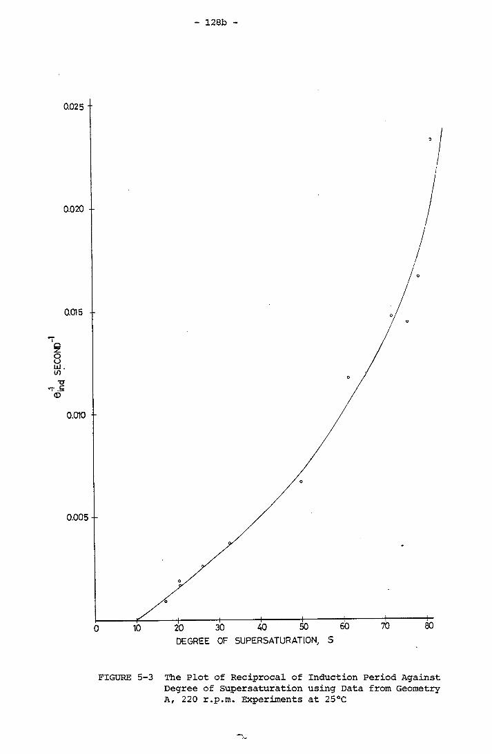
SE
CO
ND
128b
0.025 ■■
0.020 --
DEGREE OF SUPERSATURATION, S
The Plot of Reciprocal of Induction Period Against Degree of Supersaturation using Data from Geometry A, 220 r.p.m. Experiments at 25°C
FIGURE 5-3
129
constant pH because of the relatively slow rate equilibration of carbon dioxide between the gaseous phase and the solution. Therefore/significant errors are to be expected in 9 and 0 for heterogene-ind latous processes, as such no attempt was made to interprete heterogeneous nucleation data.
Using the approach of classical homogeneous nucleation theory combined with diffusion control growth of the nuclei created, nuclei growth continue to deplete the solute available until the decline of
solute concentration reaches the pH which can be detected by the pH meter and registers a finite decline of 0.01 pH unit. Again usng
Equation (5-1)
c. - cm_____c. - cm s
16n/2 3/2. . ..1/2.5/2jd v (c. - c 9.15 m in s 1 (5-10)
In the present cases, c is the solute concentration that causes a
drop of 0.01 pH unit from the initial pH. 0^ is the time taken, whichis the latent period, 9 . From Equation (5-10),1 at
for c. >> c in s
when c increases, c also increases, therefore in
mately a constant, ie is constant.
c--- is approxi-cin
Again from Equation (5-10)
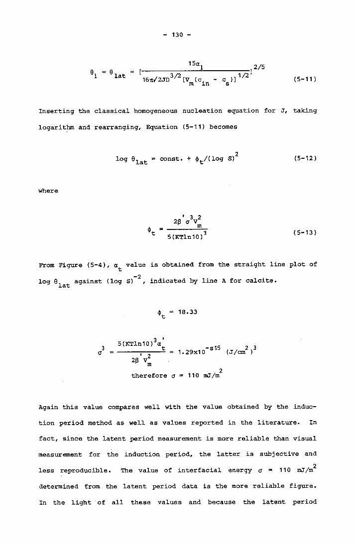
130
'1
16u/2JD3/2[V (c. - c )]V2mm s
2/5(5-11 )
Inserting the classical homogeneous nucleation equation for J, taking
logarithm and rearranging, Equation (5-11) becomes
log 9 lat const. + <j>t/(log (5-12)
where
3 2a vm5(KTln10) (5-13)
From Figure (5-4),
log 9 against (log J. 3.U
value is obtained from the straight line plot of-2S) , indicated by line A for calcite.
<b = 18.33 yt
3a5(KTlnl0)3a't „ _ _ -s15------—---- = 1.29x10
2p V2 r mtherefore a = 110 vaJ/vet
2 3(J/cm )
Again this value compares well with the value obtained by the induc
tion period method as well as values reported in the literature. In
fact, since the latent period measurement is more reliable than visual
measurement for the induction period, the latter is subjective and2less reproducible. The value of interfacial energy a = 110 mJ/m
determined from the latent period data is the more reliable figure.
In the light of all these values and because the latent period
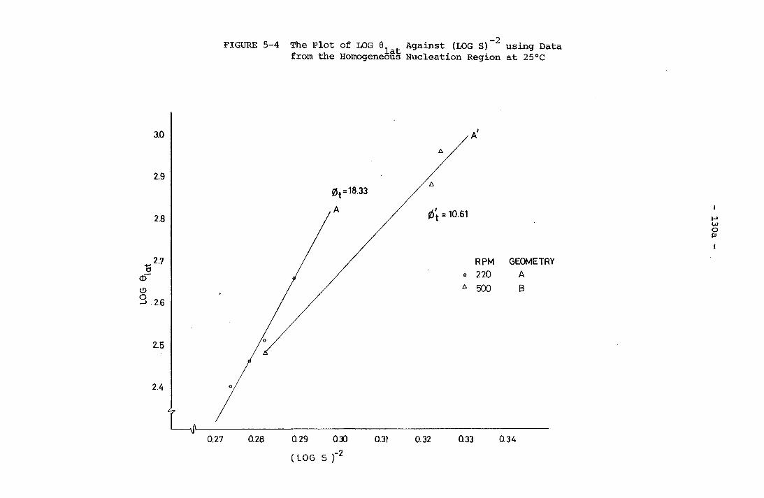
FIGURE 5-4 The Plot of LOG 6 Against (LOG S) using Data from the Homogeneous Nucleation Region at 25°C
130a
< CD
o <
COOCOCOd04COdo8d04
O'04dao04do
( LOG 5 )'

131
measurement is an additional piece of information obtained from cry
stallization experiments, it seems that there is no need to conduct
induction period measurement by separate sophisticated methods (Sec
tion (4.2. 1.3 ) ) .
Similarly, line A' gives a gradient
a 3
<b = 10.61 for the vaterite yt5 (KTlnl 0)3 4>, .. 9------—-- - = 1.43x10 13 (J/cin )
28 V K m2therefore a = 114 mJ/m
Again the value obtained is similar to the value obtained by the
induction period method.
The results of experiments to determine the effects of stirring
on both the induction period and the latent period of calcium car
bonate crystallizaton under constant initial degree of spersaturation
are plotted in Figures (5-5) and (5-6). It is difficult to be certain
whether there is a definite decline of induction and latent period
from 300 r.p.m. to 500 r.p.m., but 700 r.p.m. represents the minimum
0 and 9 before the values increase at 880 r.p.m. The effect of xnd latstirring has been reported by Mullin and Raven (1961), subsequently
Roques and Girou (1974) reported that the critical supersaturation for
nucleation decreases as the stirring speed increases, but beyond cer
tain mixing speed, critical supersaturation actually increases.
The results of magnesium experiments are shown in Figure (5-7).
The sharp decline of the induction period from 400 r.p.m. to 50 0 r.p.m. seems to suggest a significant effect of magnesium which
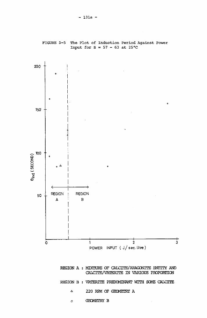
131a
FIGURE 5-5 The Plot of Induction Period Against Power Input for S = 57 - 63 at 25°C
200 "
150 -
100 --
ooUJin
-o.£<D
50 -- REGION
A
-»
REGION
B
1 2 POWER INPUT ( J/sec. litre )
REGION A : MIXTURE OF CALCITE/ARAGONITE ENTITY AND CALCITE/VATERITE IN VARIOUS PROPORTION
REGION B : VATERITE PREDOMINANT WITH SOME CALCITE
a 220 RPM OF GEOMETRY A
o GEOMETRY B
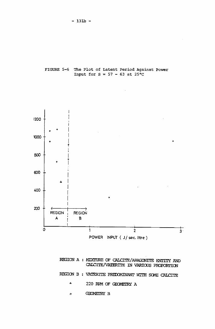
131b
FIGURE 5-6 The Plot of Latent Period Against Power Input for S = 57 - 63 at 25°C
1200 --
1000 -
800 --
600 -
400 -
A
200 -- fREGION
A
---->REGION
B
1 2
POWER INPUT ( J/sec. litre)
o
3
REGION A : MIXTURE OF CALCITE/ARAGGNITE ENTITY AND CALCITE/VATERITE IN VARIOUS PROPORTION
REGION B : VATERITE PREDOMINANT WITH SOME CALCITE
A 220 RPM OF GEOMETRY A
o GEOMETRY B
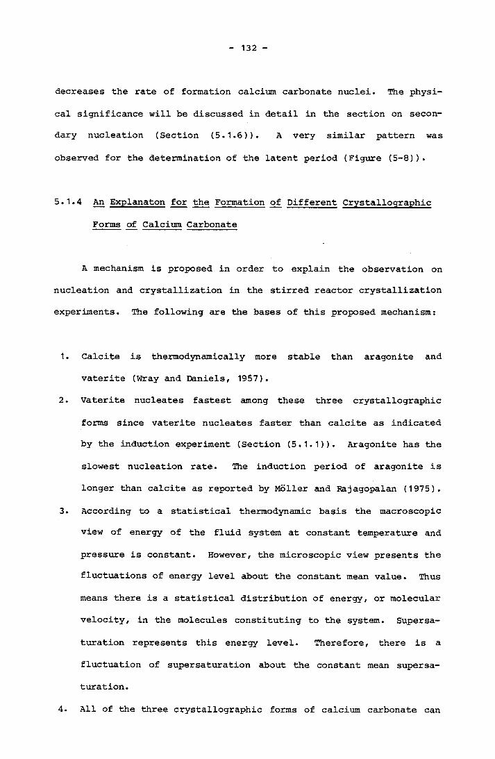
132
decreases the rate of formation calcium carbonate nuclei. The physi
cal significance will be discussed in detail in the section on secon
dary nucleation (Section (5.1.6)). A very similar pattern was
observed for the determination of the latent period (Figure (5-8)).
5.1.4 An Explanaton for the Formation of Different Crystallographic
Forms of Calcium Carbonate
A mechanism is proposed in order to explain the observation on
nucleation and crystallization in the stirred reactor crystallization
experiments. The following are the bases of this proposed mechanism:
1. Calcite is thermodynamically more stable than aragonite and
vaterite (Wray and Daniels, 1957).
2. Vaterite nucleates fastest among these three crystallographic
forms since vaterite nucleates faster than calcite as indicated
by the induction experiment (Section (5.1.1)). Aragonite has the
slowest nucleation rate. The induction period of aragonite is
longer than calcite as reported by Moller and Rajagopalan (1975).
3. According to a statistical thermodynamic basis the macroscopic
view of energy of the fluid system at constant temperature and
pressure is constant. However, the microscopic view presents the
fluctuations of energy level about the constant mean value. Thus
means there is a statistical distribution of energy, or molecular
velocity, in the molecules constituting to the system. Supersa
turation represents this energy level. Therefore, there is a
fluctuation of supersaturation about the constant mean supersa
turation.
4. All of the three crystallographic forms of calcium carbonate can
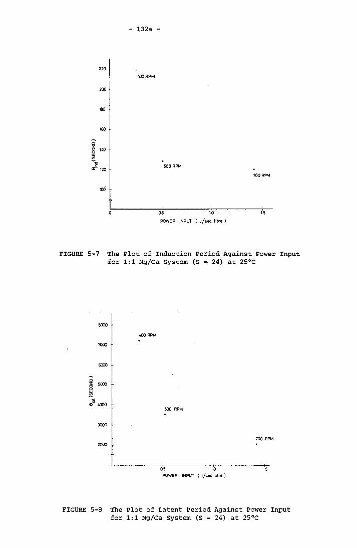
132a
FIGURE
FIGURE
220400 RPM
200 -
180
160
<sr 120 -• 500 RPM
XX) -
700 RPM
$
0 05 1.0 1.5
POWER INPUT ( j/sec. litre )
-7 The Plot of Induction Period Against Power Input for 1:1 Mg/Ca System (S = 24) at 25°C
8000
7000
6000 -
S52 4000
3000 --
2000 --
400 RPM
500 RPM
05 TOPOWER INPUT ( J/sec litre )
700 RPM
1 5
5-8 The Plot of Latent Period Against Power Input for 1:1 Mg/Ca System (S = 24) at 25°C

133
exist at the subcritical nucleus state, ie. molecular cluster or
embryo as proposed by Roques and Girou (1974).
It is clear that from the stirred reactor experiments, irrespective of
the degree of the degree of stirring, calcite will be formed at low
initial degrees of supersaturation (see Tables (4-9) and (4-10)).
This fact was reported by Brooks et. al. (1950) that slow precipita
tion rate favours the formation of calcite , whereas the more rapid
the precipitation rate, the greater the tendency to form metastable
states. The higher the inital degree of supersaturation, the faster
the precipitation rate. From the experiments, this degree of supersa
turation within the range of power input from 0.10 to 2.60 J/L s might
be 25 beyond which metastable forms will form. From the proposed
basis, the transient fluctuation of energy level represented by
degrees of supersauration at 25 and below does not provide sufficient
energy required for the formation of metastable crystallographic forms
of calcium carbonate.
When the effect of stirring was singled out from the experiments
conducted, there is a change of crystallographic form from mixtures of
calcite and acicular aragonite entity at 300 r.p.m. to vaterite
predominating at 700 r.p.m. and beyond at the degree of supersatura
tion of 57 (Figures (5-5) and (5-6 )). 400 r.p.m. - 500 r.p.m. is the
range of the transitional stirring speed (power input) where mixtures
of calcite and aragonite entity and mixtures of calcite and vaterite
in different proportions were observed. In accordance with the pro
posed basis, at S = 57.0 - 63.0, super saturation is considered high.
Therefore, the fluctuations of energy are more pronounced. Addition
ally vaterite has the fastest nucleation rate. Therefore if any

134
embryo can survive in competition with calcite, vaterite has the
greatest probability. In deed this is the case. As the stirring speed
increases, the mechanical stirring is also introducing the additional
transient increase of energy in the form of heat to the already
present transient increase of energy due to supersaturation. At 300
r.p.m. the advantage of the faster nucleation rate possessed by the
vaterite is still insignificant. However, within the range of 400
r.p.m. to 500 r.p.m. of Geometry B which also includes 220 r.p.m. of
Geometry A, the competition of all three crystallographic forms of
calcium carbonate is evident. The resulting crystal products varied
from batch to batch with different proportion of calcite/aragonite or
calcite/vat~rite under similar stirring condition and initial degree
of supersauration. However when the stirring speed was increased
beyond 500 r.p.m. the excess transient increase in energy due to stirring apparently supply the higher energy required by the formation of
metastable vaterite. Although calcite is thermodynamically more
stable then vaterite, this is off set by the faster nucleation rate of
vaterite. The overall result is therefore a majority of vaterite
rather than calcite beyond 500 r.p.m. From these experiments, it also
shows that aragonite is thermodynamically more stable than vaterite at
room temperature and moderate stirring speeds. This is the reason of
the relativey scarce deposit of vaterite in nature compared to calcite
and aragonite.
5.1.5 Secondary Nucleation of Pure Calcium Carbonate System
The final crystal numbers were plotted against stirring speed at
approximately constant initial degrees of supersauration (S = 57 - 63)
(see Figure (5-9a)). It is clear that the number of crystals
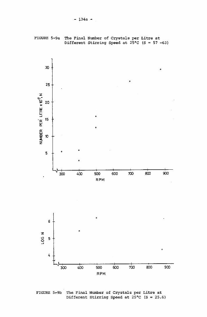
134a
FIGURE 5-9a The Final Number of Crystals per Litre atDifferent Stirring Speed at 25°C (S = 57 -63)
o 5 ..
FIGURE 5r9b The Final Number of Crystals per Litre at Different Stirring Speed at 25°C (S = 25.6)

135
increases rapidly with stirring speed from 400 r.p.m. to 700 r.p.m.
and then gradually levels off beyond 700 r.p.m.. Apparently, stirring
speed has an effect on the number of crystals generated in a batch
stirred reactor experiments. This also implies that the number of
nuclei generated is affected by the stirring speed, an indication of
the presence of secondary nucleation. At 880 r.p.m., the number of
crystals increases only sightly. If nuclei are formed from stable
clusters of molecules, the stability of molecular clusters (embryos)
can be jeopardised by vigorous stirring which breaks down the molecu
lar clusters. Therefore, the number of crystals at 880 r.p.m. is only
sightly greater than that observed at 700 r.p.m. The effect will be
more significant at low degrees of supersaturation where nuclei are
already less stable compared to medium and high degrees of supersa
turation. To examine this effect, experiments were also conducted at
low degrees of supersaturation (S = 25.6) over a range of stirring
speeds. The effect is much more pronounced than expected. The number of crystals increases by an order of magnitude from 400 to 500 r.p.m.
and decreases by order of magnitude at 880 r.p.m. (Figure (5-9b)).
In experiment PE21, crystallization of calcium carbonate was con
ducted in Geometry A stirred reactor at 220 r.p.m.. Samples were
taken to count the number of crystals (nuclei) during the course of
crystallization. The results are shown in Figure (5-10). Crystal
number increases linearly and is approximately constant beyond 25
minutes. Emergence of new spherical nuclei approximately 1 - 2 (im in
size were observed under the microscope. The birth of new nuclei
appears to stop beyond 25 minutes and the process continues with cry
stal growth predominating. This indicates insignificant secondary
nucleation as compared to crystal growth. The final crystal number is

135a
FIGURE 5-10 The Number of Crystals Counted with respect to Time for Experiment PE21 (220 r.p.m., Geometry A)
TIME ( MINUTE )

136
approximately 76% of the crystal number at the end of the nucleation
process. This implies that ageing (ripening) takes place during the
final stage of the batch crystallization process. The final crystal 7 8number is 9.13x10 per liter as compared to 1.23x10 per litre counted
during crystallization. The nucleation rate is therefore approxi
mately 30% higher compared to that calculated from the final crystal
number as defined in Section (4.3.4). This may be the case for all
the rest of the experiments on crystallization. However, not all
nuclei generated by secondary nucleation are able to survive to grow
into big crystals (Section (2.2.3)). Small nuclei seem to grow very
slowly or not at all. As a result their presence during the course of
crystallization should only incur a minimum error on growh rate con
stant based on final crystal numbers. These nuclei are most likely to
be incorporated into big crystals via ageing process and render a
smaller crystal population at the end of the process. Therefore, the
effect of ageing can be considered tolerable when the final crystal
number is used in nucleation rate calculations and crystallization
rate calculations. From this experiment, the nucleation rate appearsANto be a constant. By plotting nucleation rate (‘^g’) as defined in Sec
tion (4.5.2. 1)) for the same degree of initial supersaturation against
stirring speed expressed in power input per unit volume, a linear
relationship can be established (Figure (5-11)). Since the final cry
stal number also increases with the power input per unit volume, the
presence of secondary nucleation in the mode of nucleation is evident.
The effect of high stirring speed is more apparent when the number of
crystals is expressed in the nucleation rate. At 880 r.p.m., the
sharp decline of nucleation rate indicates the unstable environment
for viable embryos (molecular clusters) during vigorous mixing. The
experimental data presented in Table (4-7) covering different initial
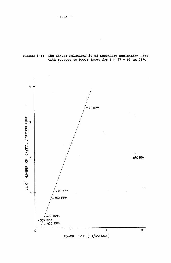
136a
FIGURE 5-11 The Linear Relationship of Secondary Nucleation Rate with respect to Power Input for S = 57 - 63 at 25°C
700 RPM
880 RPM
500 RPM
500 RPM
400 RPM
400 RPM
POWER INPUT ( j/sec litre )
0 3

137
degrees of supersaturation and stirring speeds were plotted based on
the empirical expression
where Ac
Mx
£
Jc-ms K,„ „r,(Ac)PeM (2-25) x
is substituted by S (S2 2+2 f ,[Ca ] [CO,-]
(2-25)
spis the weight concentration of calcium carbonate precipi
tated at the respective degree of supersaturation
is the energy dissipitated by the stirring per unit mass of
slurry by the stirring and is calculated from the power
number (Section (4.5.2.2))
The best fit for all this data is obtained for p=7.9 (Figure (5-
12)) which has a correlation coefficient = 0.9713. Apparently, the
effect of degree of supersaturation is still the single major parame
ter governing the rate of nucleation. The exponent of the degree of
supersaturation, p=7.9 is in agreement with the order of nucleation of
the homogeneous nucleation with respect to supersaturation defined as
S— 1. The order of nucleation n is equal to 8 (Section (5.1.2)) The
absence of significant secondary nucleation during crystallization is
because of the rapid decline of the available degree of supersatura
tion.
The linear relationship also suggests that stirrer-crystal colli
sion is responsible for secondary nucleation in stirred reactors as
suggested by Ottens et. al. (1972). Secondary nucleation studies
reported in the literature were usually studied in a MSMPR system
under steady state condition. The number of nuclei was calculated by
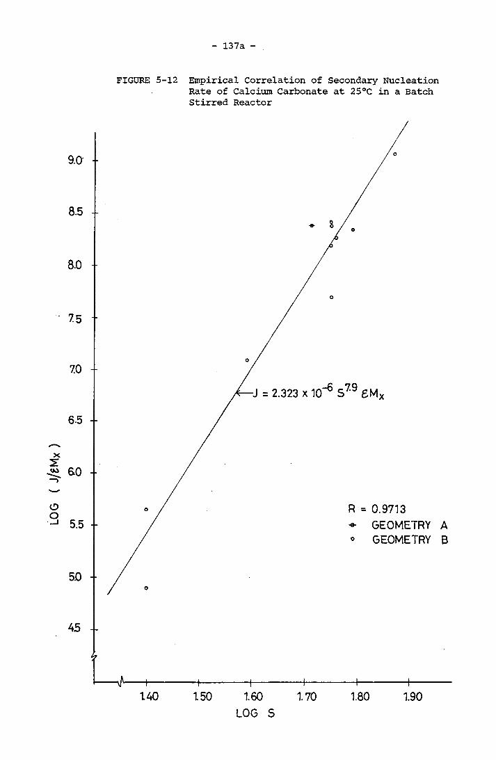
137a -
FIGURE 5-12 Empirical Correlation of Secondary Nucleation Rate of Calcium Carbonate at 25°C in a Batch Stirred Reactor
------\f-——I— ----- —(----------- —i—------- —I--------- ----- 4------------ 1—140 150 160 170 180 190
LOG S
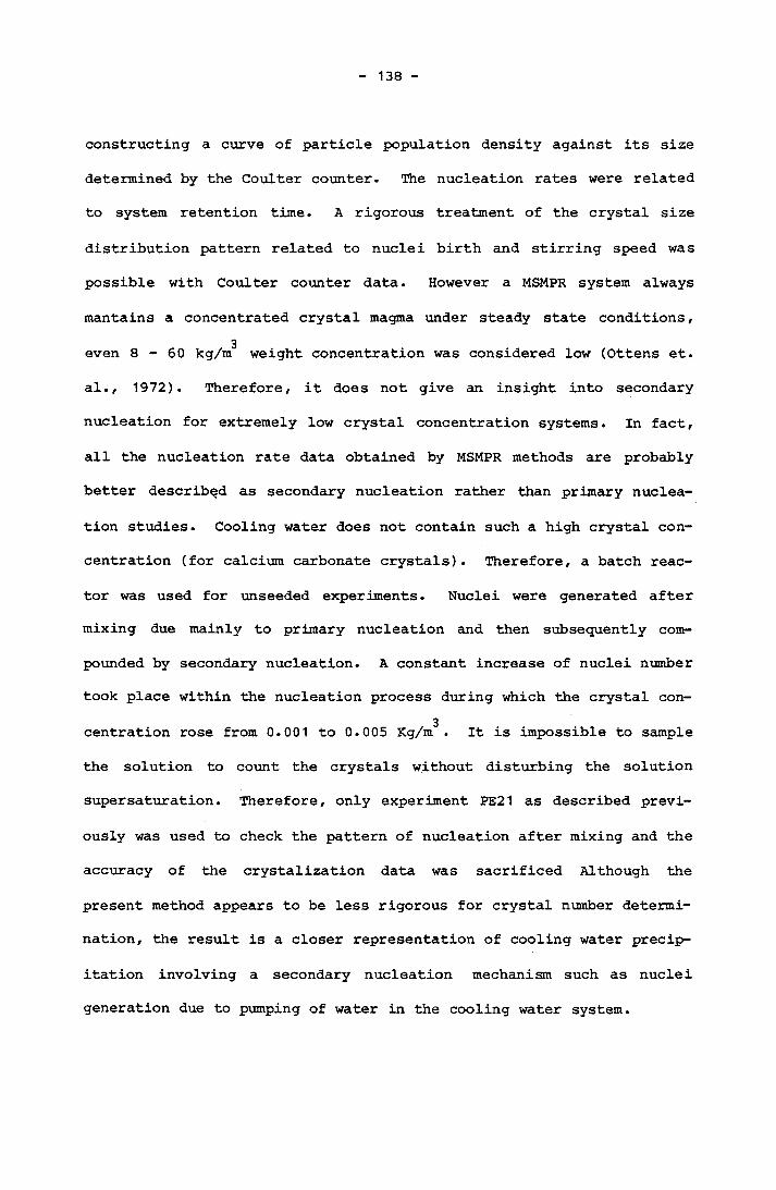
138
constructing a curve of particle population density against its size
determined by the Coulter counter. The nucleation rates were related
to system retention time. A rigorous treatment of the crystal size
distribution pattern related to nuclei birth and stirring speed was
possible with Coulter counter data. However a MSMPR system always
mantains a concentrated crystal magma under steady state conditions, 3even 8-60 kg/m weight concentration was considered low (Ottens et.
al., 1972). Therefore, it does not give an insight into secondary
nucleation for extremely low crystal concentration systems. In fact,
all the nucleation rate data obtained by MSMPR methods are probably
better described as secondary nucleation rather than primary nuclea
tion studies. Cooling water does not contain such a high crystal con
centration (for calcium carbonate crystals). Therefore, a batch reac
tor was used for unseeded experiments. Nuclei were generated after mixing due mainly to primary nucleation and then subsequently com
pounded by secondary nucleation. A constant increase of nuclei number
took place within the nucleation process during which the crystal con-3centration rose from 0.001 to 0.005 Kg/m . It is impossible to sample
the solution to count the crystals without disturbing the solution
supersaturation. Therefore, only experiment PE21 as described previ
ously was used to check the pattern of nucleation after mixing and the
accuracy of the crystalization data was sacrificed Although the
present method appears to be less rigorous for crystal number determi
nation, the result is a closer representation of cooling water precip
itation involving a secondary nucleation mechanism such as nuclei
generation due to pumping of water in the cooling water system.

139
5.1.6 Secondary Nucleation of 1:1 Mg to Ca Molar Concentration System
The presence of magnesium in 1:1 molar ratio to calcium seemed to complicate the interpretation of nucleation data. Experiments were
conducted at three different stirring speeds. Both 400 and 500 r.p.m.
experiments produced final crystals dominated by needle-like aragonite
and hexagonal shaped calcite (Plate B15 Appendix B) . Sampling for
crystal count and identification was carried out during nucleation and
crystalization of EP19 (400 r.p.m.). No crystals were observed under
microscope for 193 minutes after mixing. Beyond 193 minutes a shower
of crystals appeared and the number continued to increase rapidly as
both calcite and aragonite. At 224 minutes, another shower of cry
stals occured, this time in shower of needle-like crystal splinters
pressumbly from attrition of aragonite (Figure (5-13)). Final crystal
number is only approximately 30% of the number at 251 minutes due to
the ripening process. Therefore, the presence of aragonite, which is
always an aggregate of needle-like aragonite crystals, together with
the batchwise increase in nuclei number make secondary nucleation rate
calculation impossible.
Aragonite is thermodynamically less stable than calcite at -3 .510 * atmospheric P^ and 25°C. It was suggested by Roques and Girou
(1974) that three forms of calcium carbonate can exist at the subcrit-
ical nuclei (embryo) state. The survival probability of these embryos to nucleate and grow to macroscopic scale is determined by their ther
modynamic stability under crystallization conditions. Magnesium
cations can be adsorbed onto some preferrable forms of embryo. This
actually slows down the rate of embryo growth to reach critical nuclei
size and therefore reduces the survival probability of such embryos in
139a -
FIGURE 5-13 The Number of Crystal Counted with respect to Time for Experiment PE19 (400 r.p.m., Geometry B)
8
7
LUcr
crLUOl
2co>-cro4 -
LlOCLLUCOZD
3 -
2 -
o
o 2ND. SHOWER
o FINAL
1 o 1 ST. SHOWER
^--------- h-----------------------1-----------------------f------------ ---------h-
150 200 250 300 350
TIME ( MINUTE )
140
competition with other forms of embryo. Therefore, with this postu
late, magnesium cation have been adsorbed onto calcite and vaterite
embryos, hence reducing the number of calcite crystals and completely
inhibits the formation of vaterite. If aragonite embryos are not
affected by magnesium cation adsorption, they will have a higher sur
vival probability and grow despite being a less thermodynamically
stable entity. This postulate can also explain the general increase
in induction period in the presence of magnesium because of the
overall reduction of embryo survival probability and the rate of
embryo growth to reach critical nuclei size.
Moller and Rajagopalan (1975) proposed a different explanation of
the effect of magnesium. They suggested that small dehydrated ma<g-
nesium ions present in subcritical nucleus (embryo) of calcite distort
the lattice to such an extent that formation of stable calcite nucleus
becomes impossible at Mg/Ca > 4. The presence of smaller magnesium
cations may lead to a denser lattice structure and therefore favours
the formation of aragonite.
Precipitation of calcium carbonate was carried out in a quiescent
solution at 1 atmospheric pressure and 25°C at a initial degree of
supersaturation of 24. Only hexagonal shaped calcite crystals similar
to the 700 r.p.m. experiment were produced (Plates B12 and B13 of
Appendix B) . This conforms to Moller and Rajagopalan's finding that
the formation of aragonite requires Mg/Ca > 4. However, in stirred
experiments at 400 r.p.m. and 500 r.p.m., both aragonite and calcite
were formed for a similar initial degree of supersaturation (S = 24).
In fact the final crystal mixture was nearly 100% aragonite in the 400
r.p.m. experiment. The 500 r.p.m. experiment still produced more

141
aragonite than calcite.
The proposed mechanism in Section (5.1.4) can also be used to
explain this observation. During the initial stage of nucleation at
400 r.p.m. (PE19), an almost equal percentage of aragonite and calcite
were present. Although Mg/Ca is only 1 and not sufficiently high to
suppress the growth of calcite, the transient increase in energy in
the form of heat due to stirring has increased the probability of ara
gonite survival. The aragonite aggregates generated eventually
dispersed or produced secondary nuclei in the form of crystal
splinters under the effect of stirrer-crystal collison. The sudden
increase of aragonite crystals population allows aragonite to continue
to form new aggregates out of crystal splinters or onto the hexagonal
calcite already present. Such transitional crystal habit (aragonite
crystals on hexagonal calcite crystals) were observed in the final
crystal products (Plate B15 of Appendix B) . The nett result is the aragonite predominating crystal products.
There was no sign of aragonite in the 700 r.p.m. experiment.
Crystallization growth rate interpretations from Section (5.2.3) also
indicates no apparent retardation of the crystalliztion growth rate
constant due to the presence of magnesium. However, the secondary
nucleation rate does not obey the empirical equation derived for pure
calcium carbonate systems. Aragonite embryos did not have the chance
to grow to stable nuclei. This is probably due to the vigorous stir
ring which tends to redissolve the thermodynamically less stable ara
gonite nuclei. Because aragonite are acicular crystals, they have a
very high surface area to volume ratio which implies high dissolution
rates. The 500 r.p.m. experiment produced an aragonite dominated
142
precipitate rather than almost 100% aragonite precipitate in the case
of the 400 r.p.m. experiment, this also illustrates the effect of
increasing stirring on aragonite dissolution.
5.2 CRYSTALLIZATION OF CALCIUM CARBONATE
5.2.1 Crystal Surface and Volume Shape Factors
The weight and surface area of a crystal can be calculated from
the characteristic length measured provided the shape factors of the
crystal are known. In this project, calcium carbonate was formed in
three main crystal habits, namely rhombohedral, spherical and acicur-
lar form (Section (4.5.3.1)). Since all the acicular aragonite cry
stals formed aggregates, it is impossible to calculate either the
weight or surface area based on the characteristic lengths of the
aggregates measured, consequently no attempt was to derive the shape
factors of aragonite aggregates. Fortunately at 25°C. the calcium
carbonate precipitates from the bulk crystallization experiments are mainly discrete calcite or vaterite which are rhombodhedraL* and spher
ical respectively. The instrument used for crystal size measurement
is a computerized image analyzer (Section (4.4.3.3)) which measures
the sizes of the particle images shown on the screen from left to
right. Therefore the characteristic lengths of the particles are the
chord lengths which also depend on the orientation of the particle.
When the shape of the particle is spherical , it presents no problem
because the chord length is the diameter of the sphere, as is the case
for vaterite. The surface and volume shape factors are simply n and
n/6 respectively. However, it is not so in the case of calcite
rhombs. These calcite rhombs are monoclinic and with a inclined angle

143
of 80° (Appendix B) . Therefore the chord lengths measured from the
left to the right of the crystals are very much subject to the orien
tation of the crystals. Assuming a random orientation, the minimum
chord length measured will be the actual length of the crystals
irrespective of which side the crystals rest on the slide. This is
because the calcite crystal is trigonal with the length, breadth and thickness in equal length. The schematic representation of calcite
crystal is shown in Figure (5-14).
The maximum chord length that can be measured is apprarently the
diagonal length of the two dimensional crystal surface. From Figure
(5-14), the minimum chord length measured due to the orientation is x,
the maximum chord length measured due to the orientation is 2xcos 40°
which is equal to 1.532x. Therefore the range is from 1 to 1.532
units. Assuming a normal distribution of chord length measured within
the range, ie. ±3a = 0.532x.s
0.532x „ _Therefore a = ------ = 0.089xs 6mean (d) = x + 3a = 1.267x s
The mean of normal distribution is considered to be the most probable
chord length measured by the image analyzer for calcite rhombs subject
to random orientation.
Based on Figure (5-14), the theoretical shape factors based on
most probable chord length can be calculated as follows:
Volume = (x-y) x xsin80° + xsin80° x y xsin80° 0.9848xtan80 ° 5.671y Y0.9848Therefore y = _' : " . = 0.1736x
j • o 7 1
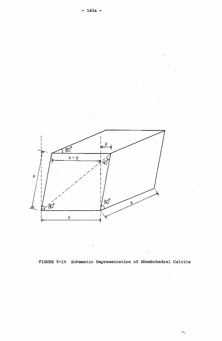
143a
FIGURE 5-14 Schematic Representation of Rhombohedral Calcite
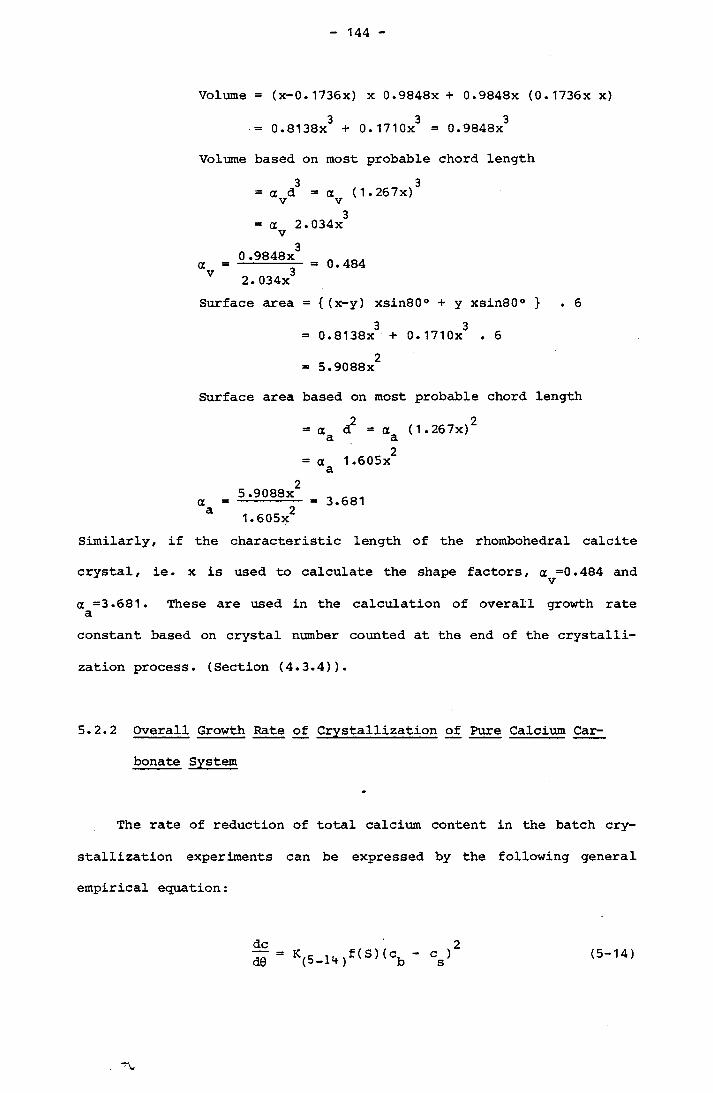
144
Volume = (x-0.1736x) x 0.9848x + 0.9848x (0.1736x x)33 30.8138X + 0. 171 Ox 0.9848X
Volume based on most probable chord length
= a d = a (1 • 267x)3 v v3= a 2.034x v
0 .9848x 0.4842.034x
Surface area = {(x-y) xsin80° + y xsin80° } . 63 3= 0.8138x + 0.1710x .62= 5.9088x
Surface area based on most probable chord length
a d a a ( 1.267x)cl
5,9088x
a 1.605x a
3.6811.605x
Similarly, if the characteristic length of the rhombohedral calcite
crystal, ie. x is used to calculate the shape factors, a =0.484 and
a =3.681. These are used in the calculation of overall growth rate aconstant based on crystal number counted at the end of the crystalli
zation process. (Section (4.3.4)).
5.2.2 Overall Growth Rate of Crystallization of Pure Calcium Car
bonate System
The rate of reduction of total calcium content in the batch cry
stallization experiments can be expressed by the following general
empirical equation:
dcd0 K,5-14,f(S)(cb (5-14)
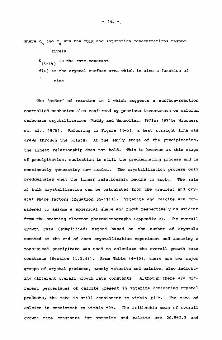
145
where c and c are the bulk and saturation concentrations respec- b stively
K is the rate constant(5-14)f(S) is the crystal surface area which is also a function of
time
The 'order' of reaction is 2 which suggests a surface-reaction
controlled mechanism also confirmed by previous investators on calcium
carbonate crystallization (Reddy and Nancollas, 1971a; 1971b; Wiechers
et. al., 1975). Referring to Figure (4-6), a best straight line was
drawn through the points. At the early stage of the precipitation,
the linear relationship does not hold. This is because at this stage
of precipitation, nucleation is still the predominating process and is
continously generating new nuclei. The crystallization process only
predominates when the linear relationship begins to apply. The rate
of bulk crystallization can be calculated from the gradient and cry
stal shape factors (Equation (4-111)). Vaterite and calcite are con
sidered to assume a spherical shape and rhomb respectively as evident
from the scanning electron photomicrographs (Appendix B). The overall
growth rate (simplified) method based on the number of crystals
counted at the end of each crystallization experiment and assuming a
mono-sized precipitate was used to calculate the overall growth rate
constants (Section (4.3.4)). From Table (4-10), there are two major
groups of crystal products, namely vaterite and calcite, also indicat
ing different overall growth rate constants. Although there are dif
ferent percentages of calcite present in vaterite dominating crystal
products, the rate is still consistent to within ±11%. The rate of
calcite is consistent to within ±9%. The arithmetic mean of overall
growth rate constants for vaterite and calcite are 20.5±2.3 and

146
2 211.5±1-0 L /min mole m respectively. Crystallization of vaterite is apparently faster than calcite.
In comparison to the simplified method, the overall growth rate method with size consideration was used to calculate the rate constants (Section (4.3.5)). There are two major difficulties in determining the surface area accurately by this method. Firstly, it is due
to the agglomerates. Although the dispersion method mentioned in Sec
tion (4.4.3.3) has significantly reduced the number of agglomerates in the samples used for crystal sizing, it is practically impossible to remove all agglomerates without also breaking the crystals. The presence of these agglomerates consistently causes an underestimation of the total crystal surface area during the crystallization process. This can be demonstrated in principle as follows::
The total weight of the sample calculated by summing over theV
entire size range was used to obtain the arbitary weight factor (n ) required to achieve the final weight of precipitate. The total cry
stal surface area of the precipitate is therefore the sample surface area obtained by summing the surface area over the entire size range
Imultiplied by n . However, when agglomerates are present, the total surface area of the precipitate will be underestimated. To illustrate this point, consider a crystal agglomerate and the final precipitate
Vis n times the weight obtained from the size of this agglomerate ofsize L . Assuming this agglomerate comprises n crystals with size aggL where L . < L . Therefore, the weight of the agglomorate isaC u dC t ciCJCJ
actually

147
Wact na 3L . v act
The arbitary factor based on weight should be
' 3 1 3n a L n Lv agg agg3 " 3na L nLv act act
(5-15)
(5-16)
Therefore, this arbitary factor should be used to obtained the actual
surface area of the precipitate.
n na L w a act
3 2n L na L agg a act n a L a agg(5-17)
The surface area based on agglomerate size L isagg
' 2A = n a L agg a agg (5-18)
Therefore the ratio of A and A isact agg
agg
n a La aggn a L a agg
aggJact (5-19)
Since L > L , therefore the actual surface area of the precipi- agg acttate is always greater than the surface area determined from the sam
ple which contains some agglomerates. This leads to a higher value of
the overall growth rate constant of the bulk crystallization of cal
cium carbonate.
148
To minimise this error, a maximum size was predetermined as the
ceiling of the size range. This is to avoid the inclusion of unrealistically large agglomerates of the sample into the size measurement.
Secondly, only grab samples were taken for the size measurement
because of the physical limitions of the instrument to count and size
the total precipitate for each experiment. This apparently will
introduce an uncertainty about whether the sample is representative of
the total precipitate. From Table (4-11), the results of the calcium
carbonate growth rate constants demonstrate a wide scatter compared to
the simplifed overall growth rate method. Experiments E22 and E23
apparently suffered the shape factor complication due to the presence
of aragonite crystals and produce a high value of the rate constant
calculated. Nevertheless, these two values are reproducible for this
kind of precipitate. The rate constants of calcite are extracted from
experiments E24, PE9 and PE11. Except E24, the growth rate constants
calculated from PE9 and PE11 are virtually identical. Therefore 3 2 217.3x10 L /mole mim m is taken as the value of calcite overall
growth rate constant determined by the size consideration method. The
arithmetic mean of calcite growth rate constants calculated from the2 2simplified overall growth rate method is 11.5±1.0 L /mole min m .
Therefore, these values from two different methods compare reasonably
well. The growth rate constant reported by Karmlerczak, et. al.3 2 2(1982) was 17.811.2x10 L /mole min m . They also recalculated the
rate constant reported by Nancollas and Reddy (1971) as 3 2 215x10 L /mole min m . The reported values suggest that the rate con
stants calculated from PE9 and PE11 based on size consideration are
identical to the seeded crystal growth method if the complications due
to agglomeration of the grab samples and non-uniform shape factors are

149
not significant. The simplified overall growth rate method registered
the lower values for the growth rate constants. Nevertheless, they
are more reproducible to with ±9% of the arithmetic mean. This repro
ducibility is attributed to the significant number of samples counted
under the microscope to acquire a statistical significance tested by 2the x test (Section (4.4.3.3J). If compared with the values of rate
constant obtained from the seeded crystal growth method (Nancollas and
Reddy, 1971) and the overall growth rate with size consideration, the
simplified method is overestimating the precipitate surface area by
making an assumption of monosized crystal. Taking PE9 for example,
the surface area of the precipitate calculated by the result of size
distribution is:
solutionIn is the factor based on the final total weight of the preci
pitate per liter solutionN is the number of crystals in class i iL is the mean size of crystals in class ii
n is the total number of size classes
a is the surface shape factor = 3.681
The surface area of precipitate per litre of solution calculated by
the simplified method is:
2= 135 cm per liter (5-20)
w
a
a 2/3aAf 2/3 Ca TCa(pa)rc v in f (5-31)

150
where a is the surface shape factor = 3.681
a is the volume shape factor = 0.484 vM is the molecular weight of calcium carbonate = 100
, 3p is the calcite density = 2.71 g/cm cT is the initial total calcium content = 0.001999 MCa. inT is the final total calcium content = 0.0008594 M af
7N is the number of crystal per liter = 3x10
Therefore
Aff = 223cm2 f
This indicates an increase of 65% surface area compared to that calcu
lated from grab samples of the final precipitate.
The overall growth rate constants of vaterite can be extracted
from experiments PE4, PE7, PE8 and PE15. Only PE7 and PE8 are repro
ducible. PE 15 is not within the normal range of data. The surface2area of the final precipitate calculated is 145 cm which is only 66%
of the final precipitate from PE4, yet these two experiments generated8almost the same crystal population (2.60x10 /L of PE15 compared to
82.94x10 /L of PE4) . As a result, the rate constant calculated is 40%3 2 2higher then the mode, namely 40.0x10 L /mole min m . From the sim
plified method (Table (4-10)), the rate constant calculated is the
smallest value and still within ±11% of the normal. The rate constant
of PE4 calculated by size consideration has a value of 3 2 228.3x10 L /mole min m . This is the closest to the arithmetic mean
growth rate constant calculated by the simplifiedmethod. No growth
rate constant of vaterite has been reported in the literature
151
therefore the reliability of these values cannot be checked. However,
using rate constant of calcite as a guideline, the overall growth rate3 3 2constant of vaterite should lie between 20x10 and 30x10 L /mole min
2m .
In conclusion, the spontaneous precipitation method present
greater difficulties to produce highly reproducible rate constants
based on true surface area calculated from size distribution measure
ment by the image analyzer for the final precipitate. However, the
simplified overall growth rate method is highly reproducible but the
crystal surface area may be overestimated. If the rate constant of3 2 2calcite crystallization is taken as 15x10 L /mole min m obtained by
3 2 2Nancollas and Reddy (1971), then the value 11.5x10 L /mole min m
calculated from the simplified method represents a 23% difference.
This is considered tolerable for kinetic growth rate determination of
such a complicated process like precipitation. The reproducibility of
seeded crystal growth rate were apparent. However, the seeded crystal
growth method requires the crystal seeds to be carefully prepared and the surface area measured. During the process of crystallizaion, the
crystal seeds continue to grow. Therefore, the transient surface area
has to be calculated by some normalization procedure (Karmlerczak, et.
al., 1982). Again the determination of true transient crystal surface
area is difficult. Consequently, although the seeded crystal growth
method was claimed to be a well controlled method to determine the
growth rate of calcium carbonate, the accuracy of the value still
suffers from the uncertainty incurred in calculating the transient
crystal surface area during the process of crystallization. The
method also requires careful preparation of the crystal seed and spe
cial instrumentation such as BET apparatus applying nitrogen
152
adsorption to determine the crystal surface area. In view of these factors, there are certainly merits in recommending the simplified overall growth rate method due to its simplicity and reproducibility.
The crystals suspension only required to be sampled at the end of the crystalization process by laboratory micropipette. The counting is
perfomed under ordinary light transmitting microscope with the sample placed in the counting chamber. The tools used are all common laboratory items and no special technique is required. The method is simple
and results reproducible. The lower (23%) growth rate constant may be
due to a consistent systematic error introduced by the micropipette during sampling. Because of the suction effect of the micropipette
during sampling, a more concentrated crystal suspension than the true concentration can be sampled consistently. As a result, the surface area of the crystals in the reactor can be overestimated and produces a lower calculated growth rate constant. Obviously the accuracy of the
growth rate constant determined by this method can be improved by modifying the sampling device to avoid the suction effect during sampling. However, a systematic error in crystal counting on a 20 jiL sample as high as 90% will only produce a 23% difference in the final value of crystal growth rate constant calculated, because the crystal number is to the one third power in Equation (4-111).
Finally, the kinetic data of the spontaneous precipitation method interpreted by overall growth rate method with size consideration can
still be valid. The accuaracy of the growth rate constants can be improved if a large quantity of the uniform precipitate suspension at
the end of the crystallization experiment can be sized by a Coulter counter. A more representative sample can prepared on a microscopic slide for size measurement by image analyzer if the crystal population
153
in the suspension is sufficiently high for crystal counting and sizing. Although spontaneous precipitation experiments have been criticised by some workers (Nancollas and Reddy, 1971; Kazmlerczak, et.
al., 1982) because of the complications due to nucleation, the present study demonstrates that the complications due to nucleation can be
ignored in the mode of crystallization and at the same time provides new insight about the effect of power input on nucleation as well as crystallization.
Both calcite and vaterite follow surface-reaction controlled
mechanism. The growth rate constants of vaterite determined by both methods are higher than calcite. Until now, theoretical calculation
of the rate constant of crystallization is still not possible although some interesting progress has been made (Nielsen, 1982). From the theories of crystal growth, rate constant comprises many fundamental parameters that are characteristic of individual crystals and its crystallographic form. Surface reaction controlled mechanism implies that processes such as adsorption and desolvation of growth unit, sur
face diffusion of growth unit, the creation of energetically favourable kinks either by surface nucleation or screw dislocation all govern the crystal growth rate. No information is available about rates of these surface processes of calcite and vaterite. However,
the nucleation rate of vaterite seems to be faster than calcite as indicated by the lower free energy required for nucleation (Section
(5.1.2)). If the surface nucleation process is singled out to be important especially at high degree of supersaturation, vaterite
should grow faster than calcite. At this stage, it is still very difficult to be certain exactly what is the controlling surface meachan- ism because the growth theories are still inadequate to allow
154
prediction of crystal growth rate from first principles. Therefore,
it is only appropriate at this stage to say that irrespective of cal- cite or vaterite crystallization, they are different crystallographic forms of sparingly soluble calcium carbonate and following an overall surface reaction controlled crystallization mechanism. Vaterite crys
tallizes faster than calcite. The surface reaction controlled mechanism is further justified because the results of overall growth rate constant are not affected by different stirring speeds. The 300 r.p.m. in Geometry B is the minimum speed required to suspend all crystals formed during crystallization. Total suspension of crystals is important so that there is no inhibition of reaction due to crystal
surface limitation. Experiment PE16 indicates an exceptionally low growth rate constant of vaterite. It is believed that this is due to
agglomeration of high crystal population and subsequently reduces the available surface area for crystal growth.
5.2.3 Formation of Different Crystal Habits in Pure Calcium Carbonate System
The presence of different habits of calcium carbonate crystal especially at high degrees of supersaturation and stirring speeds of 300 r.p.m. and beyond is evident. In the discussion on the results of
nucleation studies, qualitative explanation was attempted from the
concept of statistical thermodynamics. Crystal habits are known to be affected by many factors such as the presence of impurities , the degree of supersaturation, the temperature of crystallization, and the degree of agitation.
155
The unique shaped aragonite was observed at 25°C from Geometry A experiments and experiment PE6 using Geometry B (Tables (4-9) and (4- 10)). Under the high magnification of the scanning electron micro
scope, these aragonite crystals appeared to be the result of the continuous outward growth of crystals from a bundle of acicular aragonite
into the calcium carbonate rich environment (Plates B5 and B9 of Appendix B).
At low initial degrees of supersaturation, discrete calcite crystals were formed, for example PE 13 (Plate B6 of Appendix B) . The crystals were imperfect and showed a trail of layer growth. This pro
vides evidence to support the conventional crystal growth theories (Chapter 2).
When the initial degrees of supersaturation are 76.4 and beyond, 100% calcite was formed in the Geometry A experiment (Table (4-9)).
Similar observations on some inorganic systems were mentioned by Walton (1967). He mentioned the presence of three distinct induction regions. At low supersaturation, 'heterogeneous nucleation and discrete growth occurred. It is consistent that both Geometry A and Geometry B experiments irrespective of degrees of stirring produced a discrete calcite precipitate. As the supersaturation was increased, dentritic growth might develop. This was demonstrated by the fact
that aragonite was present when the degree of supersaturation was
below 76.4. At high supersaturation homogeneous nucleation predom
inated and the particle size of the precipitate was greatly reduced. This is in the region of 76.4 and beyond where the degree of stirring is not sufficiently vigorous to generate vaterite, a shower of relatively small calcite crystals were formed as observed in Geometry A
156
experiments.
When the crystallization experiments were conducted at 36°C, ara
gonite began to appear in long needle-like crystals aggregates in the
midst of calcite. Compared to the experiments at 25°C, this indicated
that the aragonite nuclei are more abundant and grew into discrete
acicular crystals which agglomerated during the latter stage of cry
stallization. These aggregates of aragonite were in irregular pattern
due to the result of random agglomeration compared to the consistent
pattern of aragonite aggregates observed in 25°C experiments. These
aggregates broke off easily under ultrasonication whereas the aggre
gates from 25°C experiments remained intact. At 44°C, crystals were
mainly aragonite. At 55.8°C, crystals were 100% aragonite (Plate B14
of Appendix B) . This indicates that aragonite becomes thermodynai-
cally more stable as the temperature increases. Since aragonite
formed from these bulk crystallization experiments are acicular cry
stals, they are grouped together in agglomerates. This makes a cry
stal count virtually impossible. Therefore no attempt was made to
calculate the overall growth rate constant from the experiments con
ducted at 35°C and above.
5.2.4 The Effect of Magnesium in Calcium Carbonate Bulk Crystalliza-
tion
Out of the three crystalliztion experiments on 1:1 Mg/Ca molar
ratio system, only the 700 r.p.m. experiments was able to provide the
bulk crystallization growth rate. This is because of the aragonite
agglomerates precipitated in the other two experiments which makes
crystal counts impossible. Magnesium is known to encourage the growth
of aragonite. But at the Mg/Ca ratio equals to 1, Mg is believed to
157
be still insufficient to generate aragonite predominant nuclei for bulk crystallization. Since all experiments were conducted on more or less similar initial degree of supersaturation for precipitation, the
only difference was the degree of mixing. It seems that it is this difference that triggers the otherewise thermodynaically less stable
aragonite in bulk crystallization at 25°C at 1:1 Mg/Ca. In Section (5.1.5), the formation of aragonite at 25°C was discussed.
Under scanning electron microscope, calcite appeared differently
from the simple rhombohedral habit (Plates B12 and B13 of Appendix B) . The crystals are polyhedral. They are the combination of prism with rhombohedron. Under light transmitting microscope, the crystals look like hexagonal crystals in two dimension. Similar type of crystal hibit was observed when crystals were formed without stirring.
The final appearance of crystals are due to the result of slow growth faces that bind together. In other words, the fast growth faces of the crystals grow themselves out of the formation of the final crystals (Mullin, 1972). In pure supersaturated calcium carbonate solution, all the fast growing faces disappear in the formation of rhombohedral calcite. However, when magnesium is present, certain degree
of hindrance is experienced by the fast growing faces. As a result, they survive and the crystals appear in the polyhedral form. Because
of the complex geometry of these crystals, the shape factors are dif-' 1 /3ficult to determined. However, from the overall gradient, k N , of
4experiment PE 18 (Table (4-12)), the value 1.0667x10 seems to indicate the growth rate at least is comparable to the pure calcium carbonate system. Therefore, the overall growth rate of the bulk precipitation of calcium carbonate with 1:1 Mg/Ca molar ratio at 700 r.p.m. at 25°C is considered not to be retarded by the magnesium cation.
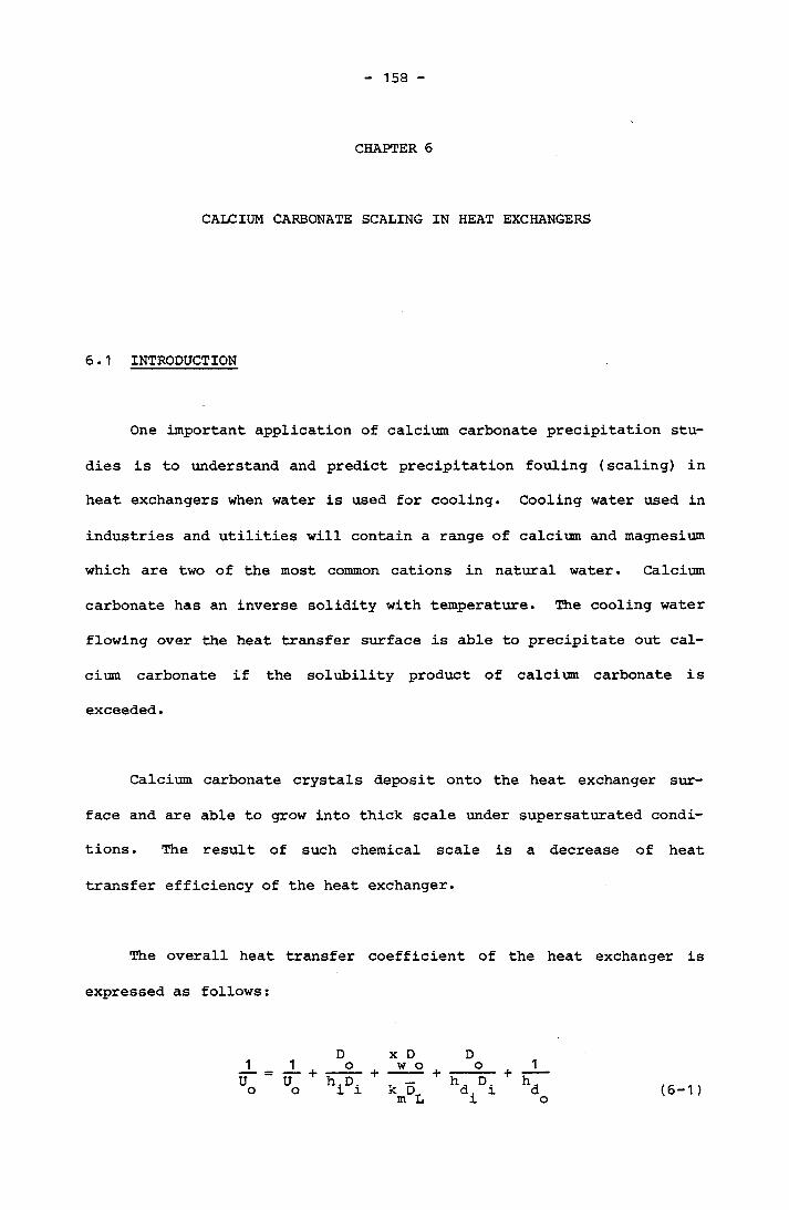
158
CHAPTER 6
CALCIUM CARBONATE SCALING IN HEAT EXCHANGERS
6.1 INTRODUCTION
One important application of calcium carbonate precipitation stu
dies is to understand and predict precipitation fouling (scaling) in
heat exchangers when water is used for cooling. Cooling water used in
industries and utilities will contain a range of calcium and magnesium
which are two of the most common cations in natural water. Calcium
carbonate has an inverse solidity with temperature. The cooling water
flowing over the heat transfer surface is able to precipitate out cal
cium carbonate if the solubility product of calcium carbonate is
exceeded.
Calcium carbonate crystals deposit onto the heat exchanger sur
face and are able to grow into thick scale under supersaturated condi
tions. The result of such chemical scale is a decrease of heat
transfer efficiency of the heat exchanger.
The overall heat transfer coefficient of the heat exchanger is
expressed as follows:
_LUo h.D. l i
x D w o+ —---- +k D m L
h D. d. l i (6-1 )

159
whereUo
hohkmxwD.lD
hdo
is the overall heat transfer coefficient based on outside diameter
is the film coefficient of the outside tube
is the film coefficient of the inside tube is the thermal conductivity of the tube wall is the thickness of the tube wall is the inside diameter of the tube
is the outside diameter of the tube is the logarithmic mean diameter of the tube
is the fouling factor of the inside tube
is the fouling factor of the outside tube.
Rf (6-2)
which is the thermal resistance due to the fouling deposit.
Therefore when the tubes are clean, is not included in the
expression. The current information on heat exchanger fouling is still scarce. Fouling factors are selected for a heat exchanger
design based on broad design guidelines as outlined in Tubular
Exchangers Manufacturers Association. T.E.M.A. Standards (1968).
Heat exchanger fouling is a complex process depending on a range
of physical and chemical factors. In the case of calcium carbonate,
the fouling factor is a function of calcium carbonate scale thickness which is also a function of time and thermal conductivity. Recently,
some efforts have been made to determine the asymptotic fouling
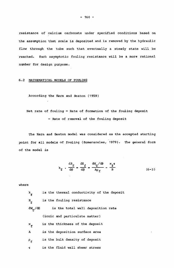
160
resistance of calcium carbonate under specified conditions based on
the assumption that scale is deposited and is removed by the hydraulic
flow through the tube such that eventually a steady state will be
reached. Such asymptotic fouling resistance will be a more rational
number for design purpose.
6.2 MATHEMATICAL MODELS OF FOULING
According the Kern and Seaton (1959)
Net rate of fouling = Rate of formation of the fouling deposit
- Rate of removal of the fouling deposit
The Kern and Seaton model was considered as the accepted starting
point for all models of fouling (Somerscales, 1979). The general form
of the model is
dR dX _ dW /d0 x r f f T f(6-3)
where
kf is the thermal conductivity of the deposit
Rf is the fouling resistance
dw /aeT is the total wall deposition rate
(ionic and particulate matter)
x f is the thickness of the deposit
A is the deposition surface area
T is the fluid wall shear stress
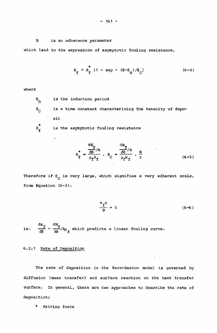
161
B is an adherence parameter
which lead to the expression of asymptotic fouling resistance,
★Rf = Rf d - exp - (0-9 )/0 ] (6-4)
where
0 is the induction periodDis a time constant characterizing the tenacity of depo
sit*
is the asymptotic fouling resistance
*
dW __id0 -/A
Pfkf
dW__ 2d 0 ‘/APf^f
BT (6-5)
Therefore if 0^ is very large, which signifies a very adherent scale,
from Equation (6-3).
xfBT
0 (6-6)
ie. —^-/Apf which predicts a linear fouling curve.
6.2.1 Rate of Deposition
The rate of deposition in the Kern-Seaton model is governed by
diffusion (mass transfer) and surface reaction on the heat transfer
surface. In general, there are two approaches to describe the rate of
deposition;
* driving force
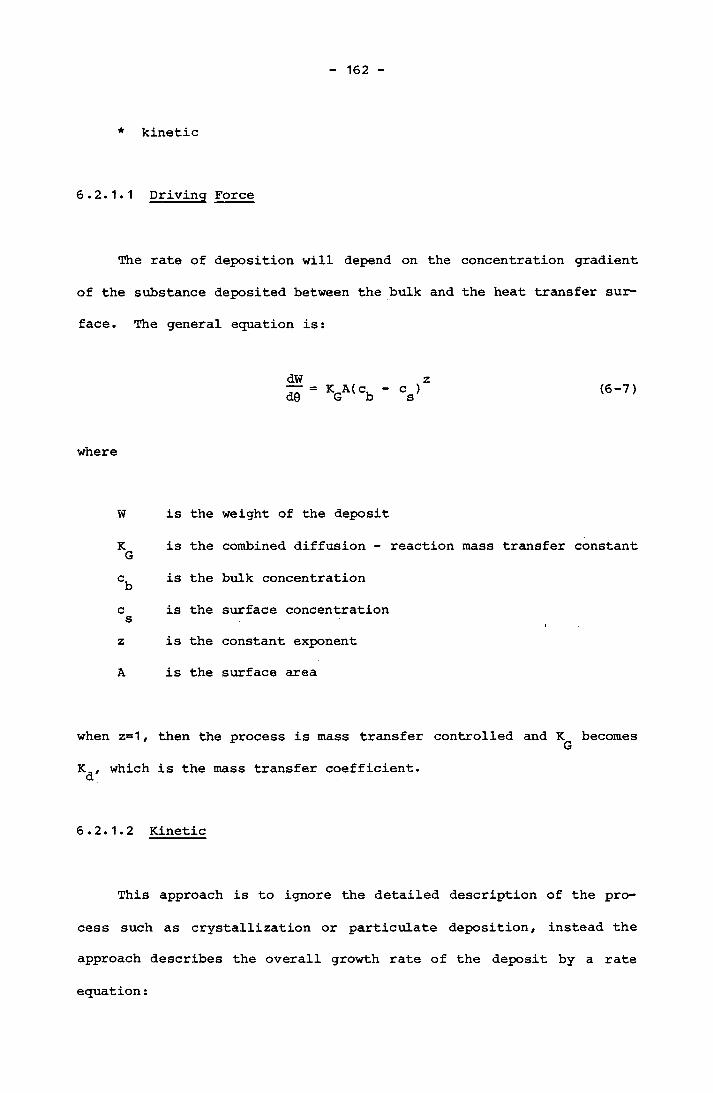
162
* kinetic
6.2.1.1 Driving Force
The rate of deposition will depend on the concentration gradient
of the substance deposited between the bulk and the heat transfer sur
face. The general equation is:
dWd0 KGA(°b (6-7)
where
w is the
K is theGcb is the
c is thesz is the
A is the
weight of the deposit
combined diffusion - reaction mass transfer constant
bulk concentration
surface concentration
constant exponent
surface area
when z=1, then the process is mass transfer controlled and K
K_, which is the mass transfer coefficient, d
becomes
6.2. 1.2 Kinetic
This approach is to ignore the detailed description of the pro
cess such as crystallization or particulate deposition, instead the
approach describes the overall growth rate of the deposit by a rate
equation:

where
K is a constant(6-8)c is the concentration of material which undergoes the reactionrn is the order of the reaction and
K is given by the Standard Arrhenius equation:r
-E/RTK = K e S (6-9)r (6-9)
where
K v is a constant (6-9 )E is the activation energy of the reaction
R is the Standard gas constant
T is the fluid/solid interface temperature (°K) at whichsthe reaction takes place
6.2.2 Rate of Removal
The rate of deposition in the heat exchanger decreases with time
mainly due to two reasons:
1. the decrease in temperature at the scale/liquid interface in the
case of constant temperature medium heating,
2. the fluid shearing effect on the deposit.
The rate of removal of calcium carbonate is generally expressed by the
equation:
164
T.W<J2) =_EK ae'r a.b (6-10)
where
dQ r is the rate of removal
is the fluid wall shear stress
is the surface area
is the adherence parameter
is the total mass deposit
B/t is extracted by Morse and Knudsen (1977) in their study as the
time constant 9^. This seems to be a good indicator of the strength
of the deposit. The larger 9the more tenacious is the deposit.
Shear stress at the fluid - deposit interface can be calculated
by the following equation:
_h dP 4 dL (6-11)
where
is the hydraulic diameter of the pipe whereh pA is the cross sectional area of the flow stream, and p is the wetted perimeter of the stream.)
— is the pressure gradient in the direction of the flow, dL
Integrating over the length L
165
APL
-2
(6-12)
where
f is the Blasius friction factorv is the fluid velocity averaged over the cross section of the pipe
p is the density of the fluidw
6.3 FACTORS AFFECTING SCALING (Suitor, et. al., 1977)
6.3.1 Velocity
Velocity of the fluid can affect the fouling process by modifying deposition and removal processes. The rate of deposition is controlled either by mass diffusion or surface reactions. In the case of scaling, the crystal growth mechanism is generally shifted from a diffusion controlled mechanism to surface reaction controlled mechanism
when the velocity is increased. This is because the overall growth rate is attributed to mass transfer for the substrate to the scale/liquid interface, followed by incorporation into the crystal
lattice by reaction at the interface. When the velocity of the fluid is increased, force convective mass transfer becomes rate-unlimiting relative to the surface reaction, therefore, the rate - controlled
mechanism is that of the surface reaction.
166
6.3.2 Temperature
The temperature of the liquid that contains inversely soluble salts such as CaCO^, CaSO^ etc is critical to precipitation processes. When the temperature is sufficiently high that the solubility product
of the salt is exceeded, supersaturation is created and eventually will lead to precipitation.
Temperature of the heat transfer surface therefore also strongly affects the scaling process. With s-ufficiently high temperature, local super saturation can be created. In addition, the rate of cry
stallization is governed by temperature in the form of an Arrhenius equation, therefore the higher the temperature, the faster is the rate of scaling. In the case of a constant temperature heating medium system, the temperature at the scale/liquid interface will gradually decrease when scale builds up. This will lead to a natural decrease in the rate of scaling.
6.3.3 Tube Surface •
The structure of the tube surface may be important for the ini
tial nucleation of the scaling process. If cavities of appropriate size are present on the tube surface, scaling crystals nuclei can be
retained in the cavity and subsequently grow into crystals. In other words, crystallization sites are available on the tube surface.
Additionally if scaling chemicals precipitate onto the surface via a deposition fouling process, they have to overcome the energy
barrier at the tube surface before the particles can get to the wall
167
(Ruckenstein and Prieve, 1973; Spielman and Friedlander, 1974;
Dahneke, 1973; Bowen et. al., 1976). This energy barrier is the
result of London-van der Waals and electrical double layer interaction
forces. The latter can be attractive or repulsive depending on the
charges of the particles and wall. Whereas London-van der Waals
forces are always attractive.
6.3.4 Water Chemistry
Water chemistry is the primary factor which controls scaling. If
the water is supersaturated with scaling'-potential chemicals, then the
water is likely to foul the heat exchanger. The primary driving force
is therefore the degree of supersaturation of scaling chemicals. The
degree of supersaturation of a specific scaling chemical is governed
by temperature, pH, dissolved solids and other chemical species
present. For example, CaCO^ supersaturation is strongly controlled by* _
pH which determines the concentration distribution of ^CC^, HCO^ and 2-COg species as described in chapter 3. If the solubility product of
CaCO^ is exceeded, the water is supersaturated with CaCO^ • The pres
ence of other hardness species such as Mg also alter the degree of
supersaturation of CaCC>3 . The effect of mixtures of salts can be sig*-
nificant due to formation of complex species, hence changing the con
centration driving force.
6.4 CALCIUM CARBONATE SATURATION INDEXES
The solubility of calcium carbonate is the primary cause of cal
cium carbonate scaling in heat exchangers, conversely low concentrations can cause corrosivity of water. Attempts to define corrosivity
168
and scaling have focused on predicting the ability of the water to
deposit CaCO^ films. Several indexes of calcium carbonate saturation
have been proposed. The existence of many indexes shows that no sin
gle index has proved to be entirely satisfactory. Recently Rossum and
Merrill had made an evaluation on six calcium carbonate saturation
indexes and discussed the reliability of the indexes for predicting
the water's capacity for CaCO^ deposition or dissolution. (Rossum and
Merrill, 1983).
6.4.1 Langelier Index (LI)
This is the most commonly used index. Langelier (1936) developed the
concept of a Saturation index, often referred to as the Langelier
Index (LI) to characterise a water as to whether it is scale forming
or scale dissolving.
LI = pH - pH (6-13)actual s
The PKactua^ value is the pH value of the water. pHg is defined by
Langelier as 'pH value at saturation' to mean that theoretical pH
value at which in water of a given alkalinity and calcium content
would be just saturated with CaCO^•
2-[CO^ ] can be expressed in terms of measured alkalinity (Equation
(3-48)) and substituted into the calcium carbonate solubility product
equation. The corresponding [H+] to satisfy calcium carbonate satura
tion is calculated as pH . The trial pH can be calculated from the
equation.
169
2 +pH = pK - pK + p[Ca ] + s 2 spp([Aik] - [0H~] + [H+] ) + log(1+2K /[H+] ) - log f (6-14)s s 2 s m
where
[Aik] is the total alkalinity in equivalents per litre
[ ] designates a saturated molar concentration
For most waters, a number of simplifying assumptions can be made in
specific pH ranges:
(1) For 9.5 < pH < 10.3, hydrogen and hydroxide ion concentra
tions are negligible in the term ( [Aik]-[OH ] + [H+] ).s s
pH = pK - pK + p[Ca^+] + p[Alk] s 2 sp
+ log( 1+2K /[H+] ) - log f (6-15)2 s m
This equation has to be solved by an iterative technique
(2) For 6.5 < pH < 9.5, the term 2K /[H+] is negligible2 s
2 +pHg = pK2 - Pkgp + p[Ca ] + p[Alk] - log f^ (6-16)
(3) For pH < 6.5 the terms 2K2/[H ]g and [OH ]g are negligible
2+ +pH = p^ - pK + p[Ca ] + p( [Aik] + [H ] ) - log f^
Again has to be solved by an iterative technique.
(6-17)
170
A positive LI indicates that the water is scale forming, a nega
tive LI indicates that the water is scale dissolving.
Snoeyink and Jenkins (1980) have redefined pH as the pH of thessystem if saturated with CaCO^ at the measured calcium and bicarbonate
concentrations instead of basing the index on alkalinity. This sim
plifies the calculation of pH . According to Rossum and Merills(1983), such an index (LI^) better relates to a water's capacity to
precipitate CaCO^ than the LI index.
6.4.2 Ryznar Stability Index (RI)
Ryznar Stability Index was proposed by J.W. Ryznar (1944) as an empir
ical index to indicate the state of water. The index is equal to
2pHs~pH where pH^ is the Langelier Saturation pH and pH is the meas
ured pH value of the water. Ryznar correlates this index with experi
mental results as well as field data and concluded that below 6.0 the
water is scale-forming while beyond 7.0 the water is corrosive.
Therefore, the water is considered stable between index number of 6.0 and 7.0.
6.4.3 Driving Force Index (DFI)
This is defined as
DFI2+ — [Ca ] [CO ] ________ 3_Ksp (6-18)
A DFI of 1.0 indicates the water is saturated with CaCO. A number

171
greater than 1.0 indicates supersaturation, whereas a number less than
1.0 denotes an undersaturated water.♦
6.4.4 Aggressiveness Index (AI)
This index was developed for asbestos - cement pipe and water tempera
tures in the range of 4°C-27°C. It is defined as:
AI = pH + log^Q{Ca2 }{Alk} (6-19)
where {} is designated for concentration of the component in mg
CaC03/L.
Waters with an AI less than 10 are aggressive, between 10 and 12
waters are moderately aggressive, and waters which exceed an AI of 12
are considered to be non aggressive.
6.4.5 Momentary Excess (ME)
This index was developed by J.F. Dye ( 1952) and stated that ME
was equal to the moles of CaCO^ that must precipitate to satisfy the
following equation:
([Ca2+] - ME)([C02“] - ME) Ksp (6-20)
A positive ME denotes a supersaturated water, a negative ME denotes a
corrosive water, and a zero ME denotes a water saturated with CaCO^.
172
6.4.6 Calcium Carbonate Precipitation Potential (CCPP)
This index has been used by Merrill and Sanks (Merrill, 1976; Merrill
and Sanks, 1977a; 1977b; 1978) to indicate theoretical quantity of
CaCO^ that can precipitate from supersaturated waters or are dissolved
by undersaturated waters. During the process of precipitation the
concentrations of calcium and carbonic species change. Therefore the
equilibrium concentrations at the end of the process will not be the
same as described by pH of the Langelier Index which assumes the ini-stial calcium concentration and the initial total alkalinity.
During CaCO^ precipitation, the equivalents of calcium carbonate
precipitated is equal to alkalinity precipitated (Lowenthall and
Marais, 1976). An equal number of equivalents of calcium and alkaline
are precipitated as calcium carbonate. Therefore, at equilibrium
2(.[Ca2 + ] . - [Ca2+] ) = Aik. - Aik (6-21)l eq i eq
2+ 2 +where [Ca ]. and [Ca ] are initial and equilibrium calcium molar l eqconcentrations.
Aik and Aik are initial and equilibrium total alkalinity in i eqequivalents per litre.
The index is expressed as follows:
CCPP = 50000 (Aik - Aik ) (6-22)i eq
where CCPP is in mg/CaCO^
Aik has to be calculated by trial and error from the following eq
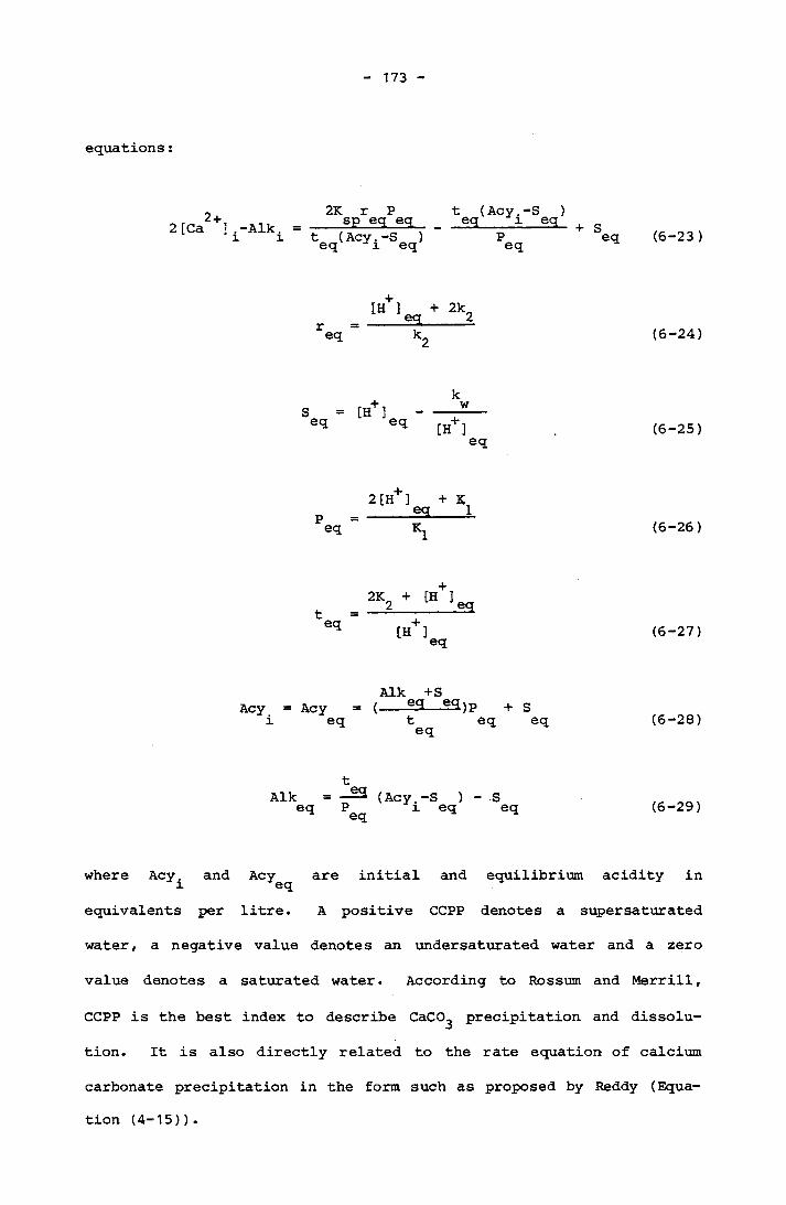
173
equations:
0 2K r P t (Acy.-S )2[Ca2+] .-Aik. = „ ,?■1i i t (Acy. -S ) Peq i eq eq
+ S (6-23 )
req[H+] + 2k____ eq_____ Z
(6-24)
Seq
2 [H+] + Kp = —____SSL__ 1eq Kl
(6-25)
(6-26)
teq2K2 + [H ]eg
[H+] (6-27)
Aik +SAcy = Acy = (-- ^2—®2)p + si eq t eq eq (6-28)eq
Aikeq —^2 (Acy.-S ) P i eq Seq (6-29)
where Acy. and Acy are initial and equilibrium acidity inl eqequivalents per litre. A positive CCPP denotes a supersaturated
water, a negative value denotes an undersaturated water and a zero
value denotes a saturated water. According to Rossum and Merrill,
CCPP is the best index to describe CaCO^ precipitation and dissolu
tion. It is also directly related to the rate equation of calcium
carbonate precipitation in the form such as proposed by Reddy (Equa
tion (4-15)) .
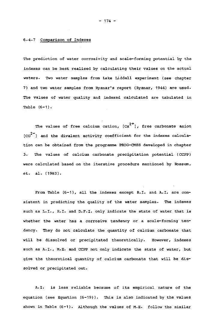
174
6.4.7 Comparison of Indexes
The prediction of water corrosivity and scale-forming potential by the
indexes can be best realised by calculating their values on the actual
waters. Two water samples from Lake Liddell experiment (see chapter
7) and two water samples from Ryznar's report (Ryznar, 1944) are used.
The values of water quality and indexed calculated are tabulated in
Table (6-1).
2 +The values of free calcium cation/ [Ca ] , free carbonate anion2-[CO ] and the divalent activity coefficient for the indexes calcula
tion can be obtained from the programme PROG-CMSS developed in chapter
3. The values of calcium carbonate precipitation potential (CCPP)
were calculated based on the iterative procedure mentioned by Rossum,
et. al. (1983).
From Table (6-1), all the indexes except R.I. and A.I. are con
sistent in predicting the quality of the water samples. The indexes
such as L.I./ R.I. and D.F.I. only indicate the state of water that is
whether the water has a corrosive tendency or a scale-forming ten
dency. They do not calculate the quantity of calcium carbonate that
will be dissolved or precipitated theoretically. However, indexes
such as A. I., M.E. and CCPP not only indicate the state of water, but
give the theoretical quantity of calcium carbonate that will be dis
solved or precipitated out.
A. I. is less reliable because of its empirical nature of the
equation (see Equation (6-19)). This is also indicated by the values
shown in Table (6-1). Although the values of M.E. follow the similar

174a
TABLE 6-1 The Comparison of Calcium Carbonate Indexes
WaterSample
WaterQuality
Lake Liddell Expt. 5
Lake Liddell Expt. 7
La Grange, 111 Well Water
La Grange, 11 1 Well Water
Total Calcium (ppm CaCO^)
264 331 526 526
Total Magnesium (ppm CaCO^)
261 344 326 326
Total Alkalinity (ppm CaCO^)
126 362 397 397
Sulphate (ppm SOJ")
480 663 450 450
Chloride (ppm Cl )
346 328 51 51
oTemperature ( C) 24.7 25.5 15 60
PH 7.90 8.52 6.8 6.8
L. I. 0.28 1.37 -0.23 0.56
R. I. 7.34 5.78 7.26 5.68
O H 1.86 22.2 0.59 3.64
A. I.(ppm CaCO^ )
M. E.(mole/L CaCC>3 )
12.3
6.62 x 10"6
13.4
1.72 x 10“4
12.0
-2.00 x 10“6
12.0
4.12 x 10~6
CCPP(ppm CaCO )
3
4.3 56.6 -44.4 96.8

175
direction compared to CCPP and other indexess, it is based on a less
rigorous theoretical basis compared to CCPP. Hitherto, CCPP is the
best index to describe calcium carbonate precipitation and dissolu
tions (Rossum and Merrill, 1983) for the value not only indicates the
state of water, but also suggests a theoretical quantity of calcium
carbonate precipitation and dissolution. The values of these indexes
are a good starting point to predict the impact of water onto heat
exchangers. However a more rigorous treatment is required in order to
predict the behaviour of the water more precisely because of other
physical factors involved such as temperature, tube surface and velo
city of the fluid. In fact one major approach of modeling of calcium
carbonate scaling in the heat exchangers follows the line of empirical
growth rate equation of the scale in the form of Arrhenius rate equa
tion with little or no emphasis on the chemistry of the water (Knudsen
and Story, 1975; Morse and Knudsen, 1977). The review of calcium car
bonate scaling models are given in the following section.
6.5 LITERATURE REVIEW ON CALCIUM CARBONATE SCALING (PRECIPITATION
The first fouling study published is on chemical deposition in eva
porators by McCabe and Robinson (1924). They proposed the mathemati
cal model under constant heat flux:
FOULING)
(6-30)
U1_2 (6-31 ) 0 (6-31 )
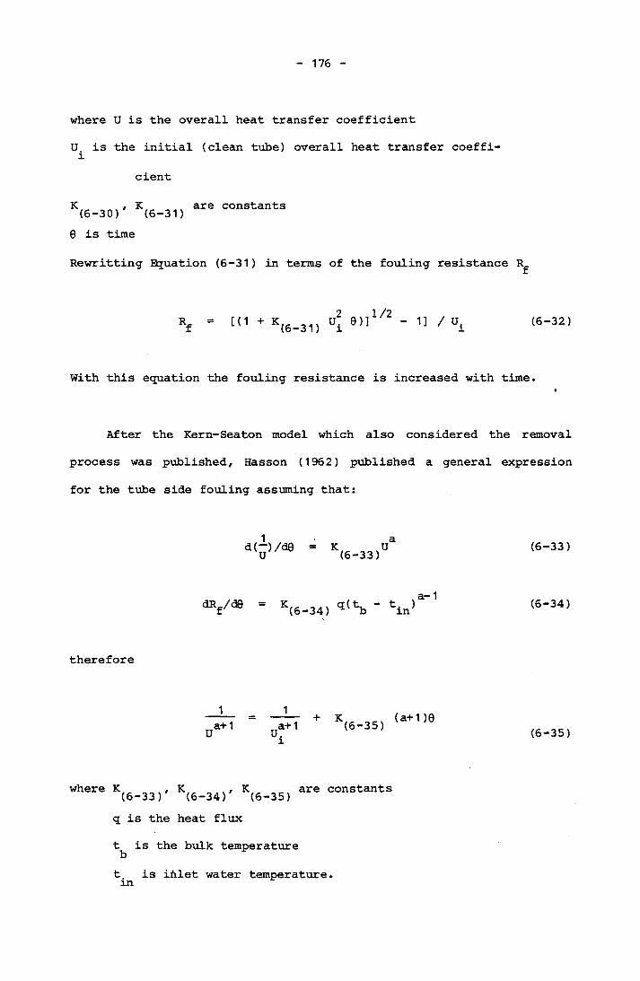
176
where U is the overall heat transfer coefficient
U is the initial (clean tube) overall heat transfer coeffi- icient
K , K are constants(6-30) (6-31)0 is time
Rewritting Equation (6-31) in terms of the fouling resistance R
[(1 + K(6-31) Ui 9)]W2 - 11 7 Ui (6-32)
With this equation the fouling resistance is increased with time,
After the Kern-Seaton model which also considered the removal
process was published, Hasson (1962) published a general expression
for the tube side fouling assuming that:
d(“)/d0 K (6-33)aU (6-33)
dRf/d0 K q( t - t. )(6-34) b ma- 1 (6-34)
therefore
K „v (a+1)0 (6-35) (6-35)
Whele K(6-33>' K<6-34)' K(6-35) ^ constants q is the heat flux
t^ is the bulk temperature
t is inlet water temperature, in

177
The experimental data fitted to this model resulted in a value of
2.5 for a at low velocity. With higher velocity such as 1m/s, the
removal process became important. However Hasson suggested that the
use of a higher value a would correlate the higher velocity data with
the low velocity data confirming the unlimited growth model.
Hasson also proposed the deposition process of CaCO
diffusion theory of crystallization,3 based on the
dWd0 K A G (c -c ) b s (6-36 )
where A is the surface
is the overall growth rate
c is the bulk concentration bc is the saturated concentration s
Assuming a first-order surface reaction.
_L _ _L J_K “ K + K (6-37)G d r
where K is the mass transfer coefficient dK is the surface reaction rate coefficient for the CaCO r 3
molecules to be arranged into crystal lattice
is evaluated empirically by
, 0.83 0.53Sh = K d/D = 0.023 Re Sc (6-38)d
and

178
Kr (6-39)
where Sh is the Sherwood number
d is the particle diameter
D is the molecular diffusivity
Re is the Reynolds number
Sc is the Schmidt number
K is a constant(6-39)E is the activation energy
R is the universal gas constantoTg is the surface temperature, K
At low velocity, the experimental data fitted well. At higher
velocity the model breaks down because of the absence of a removal
term and also the crystallization process tends to be surface reaction
controlled. The reaction was suggested to be second order by Nancol-
las and Reddy (Reddy and Nancollas, 1971; Nancollas and Reddy, 1971).
Reitzer (1964) developed the fouling rate equation based on the
inverse solubility of the salt, crystallization velocity, scale pro
perties and heat transfer conditions. He introduced the linear rela
tionship of concentration of inversely soluble salt with temperature.
c (6-40)
where c is concentrationK is a constant(6-40)b is the slope of the solubility curve
t is the temperature
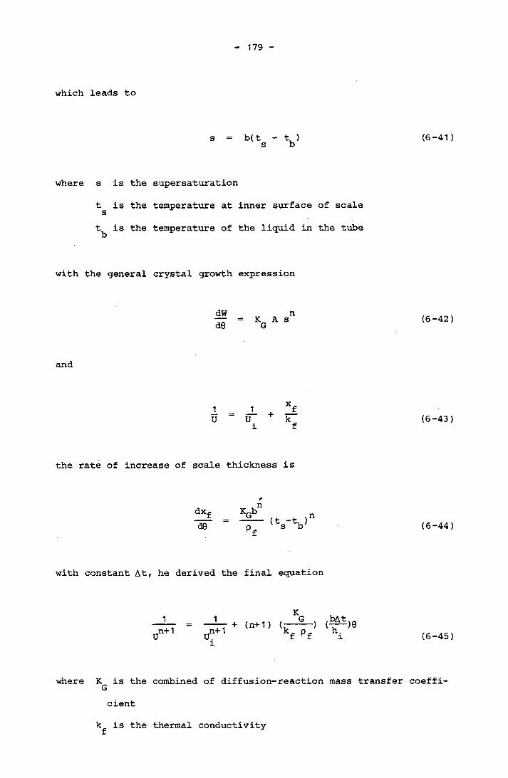
179
which leads to
s = b(t - t ) s b
where s is the supersaturation
t is the temperature at inner surface of scale s
t is the temperature of the liquid in the tube
with the general crystal growth expression
and
dWd0
nK A s G
the rate of increase of scale thickness is
dXf KQb ‘VS’
with constant At, he derived the final equation
1n+1U
(n+1 )
where KG is the combined of diffusion-reaction mass transfer
cient
is the thermal conductivity
(6-41 )
(6-42)
(6-43)
(6-44)
(6-45)
coeffi-
180
At is the total temperature drop from heating to cooling medium
Pf is the scale density
when n=1, Equation (6-44) becomes
2bK At~2 + ^nr9U pf f i1 (6-46 )
which is similar to ~1 1y + |39 derived by McCabe and Robinson whereU U.
|3 is a constant,
Under constant heat flux condition the final equation becomes
2U >r'"1
0 (6-47)
where q is the heat load.
For unsaturated solutions, the final equation derived is
1_U (6-48)
where c^ is the concentration of liquid and c* 1 is the hypothetical
concentration of liquid saturated with scaling component at t^.
Hasson (1968) measured the rate of CaCO^ scale deposition on the
surface of annular constant heat flux exchanger, with the scale sur
face temperature maintained constant irrespective of scale layer
thickness. Effects of flow velocity, scale surface temperature and
181
water composition were examined according to the rate model presented.— 2+The rate model considered the mass transfer of HCO^ and Ca toward
2+the reaction surface and followed by surface reaction between Ca and2-CO3 to form CaCO^* The backward diffusion rate of dissolved C02
formed during the reaction is also taken into account.
Overall reactions occurring in the crystallization of CaCO^ scale
are represented by
2HC03 ■> + CO, + H2° (6-49)
Ca 2+ + CO CaCO (s) 3 (6-50)
mass transfer coefficient was obtained from heat transfer correlation
derived experimentally,
h D i ekw
0.0608 (Re) 0.716f (6-51 )
where De(Re) f
(pr)f
kw
is the equivalent diameter of annular flow passage
is the Reynolds number of water based on average film tem
perature
is the Prandtl number of water based on average film tem
perature
is the thermal conductivity of water
combined with j-factor analogy between heat and mass transfer

182
Kd h.i <FV • (pr/sc)fP (6-52)
where C is the specific heat of water P
p is the density of water
(Sc)^ is the Schmidt number based on average film thickness
K is the mass transfer of the species considered d
oThe experiment was carried out at surface temperatures 6 7 C to
85°C and Reynolds numbers from 13/000 to 42,000. CaCO^ deposition is2+mainly controlled by the forward diffusion rate of Ca and HCO^ ions.
In certain cases it is also controlled by the backward diffusion rate
of dissolved CO^ formed during the reaction.
Taborek et. al. (1972a, 1972b) reviewed the mechanisms of foul
ing and established a mathematical model verified by a massive data
bank accumulated by Heat Transfer Research Incorporated (HTRI). The
model also includes a removal term, probability function of the scale
as well as the water characterization factor to account for the effect
of water chemistry.
For
d( x /k f f)d9 ♦d“ *r
*d = K(6-53) Pd (Q) exP(~E/RV (6-53)
(6-54 )<J> (6-54)
183
where ^ and ^ ^ are constants
P is the probability function dQ is the water characterization factor which is a function
of Langelier Index
<J> is a function of the deposit structure
t is the shear stress of the flow
m is a constant to be determined experimentally
Xf is the thickeness of deposit
k^ is the thermal conductivity of deposit
<J) is the rate of deposition
<b is the rate of removal r
Equation (6-53) is derived from the general reaction controlled
expression
K K(6-53) r (c ) rn
where c is the reaction concentration described by P and Q. If im=1, r dequations (6-22) and (6-23) can be combined
R*f(1—e"B'9)
*where ‘(6-53) d (Q) exp(-E/RT ) s'f (6-54) x/<\>
and B' XK,_ C„ 7(6-54) f 4>
(6-55)
(6-56)
(6-57)
184
Watkinson and Martinez (1975) studied scaling of calcium car
bonate inside copper tubes. The scaling process was studied under
accelerated scaling conditions. They also derived the mathematical
model based on Kern-Seaton model. The deposition term was a generali
zation of the Reitzer model,
dx __fde
r .n—■ (c-c. ) o _ i (6-58)
where is crystallization rate constant in terms of wall temperature
t and including a removal term: w
where a is a constant and r=fv p/2.
(6-59)
The asymptotic fouling resistance can be obtained by setting*
0 in Equation (6-58) and putting Rf = x^/k^.d0
R- d + R. h.) f f i
2 b K (t - t x r w b)
K(6-40)kf fv pfp (6-60 )
Knudsen and story (1975) studied the effect of heat transfer surface
temperature on the scaling behaviour of simulated cooling tower water
using equations (6-55), (6-56) and (6-57). Under constant heat flux
condition, they derived the final results on asymptotic fouling resis
tance with respect to surface temperature:

185
* 1 1R = (3 x 10 ) exp( - 11000/RT ) (6-61)f s
The coefficient (3x10^) is specific for the experiments carried out
and embodies the velocity, water quality, and scale properties which
were constants for all runs.
Morse and Knudsen (1977) investigated the effect of alkalinity on
the scaling of simulated cooling tower water also based on the Taborek
et. al. ( 1972a, 1972b) model. They noticed that there was fre
quently a delay time between the start of the run and the formation of
deposit. Therefore, in order to fit the data to Equation (6-55), the
equation was modified to the form
R. = R* [1 - exp(-(0-9 )/0 )] (6-62)r r Dc
where 9 is the delay time Dx9 = 1/B' is the time constant where B' = 1C ^ „ k ~c (6-54) f(|;
The alkalinities studied were from 115 to 187 mg/L CaCO^. Flow
rate, bulk and surface temperatures were maintained constant for all runs. The velocity was 1.04 m/s through the annular section. Surface
temperature was around 70° C. Exact correlation of alkalinities and
fouling resistance could not be established. They concluded that the
actual effect of alkalinity is complex since changing alkalinity will
change water quality and also will change the composition of the depo
sited scale.

186
Hasson et. al. (1975) considered the kinetic of CaCO^ crystall
ization and mass transfer of ionic species. The approach is similar
to the diffusion theory of crystallization which leads to the general
crystal growth rate equation:1 dWA d0 (c.
K (c G D
(6-63)
(6-64)
(6-65)
where A is the surface area
c is the bulk concentration of the species bc. is the interfacial concentrationi
c is the saturated concentration sK is mass transfer coefficient dK is surface reaction coefficient rK is the overall growth rate Gz,n is the order of reaction for surface controlled and overall
reaction respectively
In Hasson's paper, Equation (6-64) became
1 dWA d0
, 2+ 2- K { [Ca ] . [CO, ] r l 3 K }sp (6-66 )
as the crystallization rate equation well established (Reddy and Nan-
collas, 1971; Nancollas and Reddy, 1971; Grazit and Hasson, 1975;
Wiechers, et. al., 1975).
Equation (6-63) became
1dW 2“ 2“ 2+ 2 +a ae = Ka{ [co3 1 ” tco3 h > = Kd{ [Ca 1 ‘ tCa h ><6-67>

187
Combine equations (6-65) and (6-67) and calculate K which is the con-dvective diffusion coefficient of CaCO^ from correlation (Linton and
Sherwood, 1950).
2/3~~ Sc 0.023Re-0. 17 (6-68)
where v is the flow velocity in tube
Re is the Reynolds number
Sc is the Schmidt number
The final simplified equation, with the unknown interfacial con
centrations eliminated from equations (6-65) and (6-67),
1 <*WA d0[Ca ][CO ]
K [Ca (6-69)
for pH. The chemical species were calculated from the chemistry of
CO^ “ H^O system. K'Sp -*-s t^ie solubility product of CaCO^ after temr- perature and total dissolved solids correction.
For low pH values, the diffusion equations are
if = t<ihcV ' [HCVi>= K { [CO ] . - [CO ]} d 2 l 2= K, { [Ca2 + ] - [Ca2 + ] .} (6-70)d i
The final simplified equation is
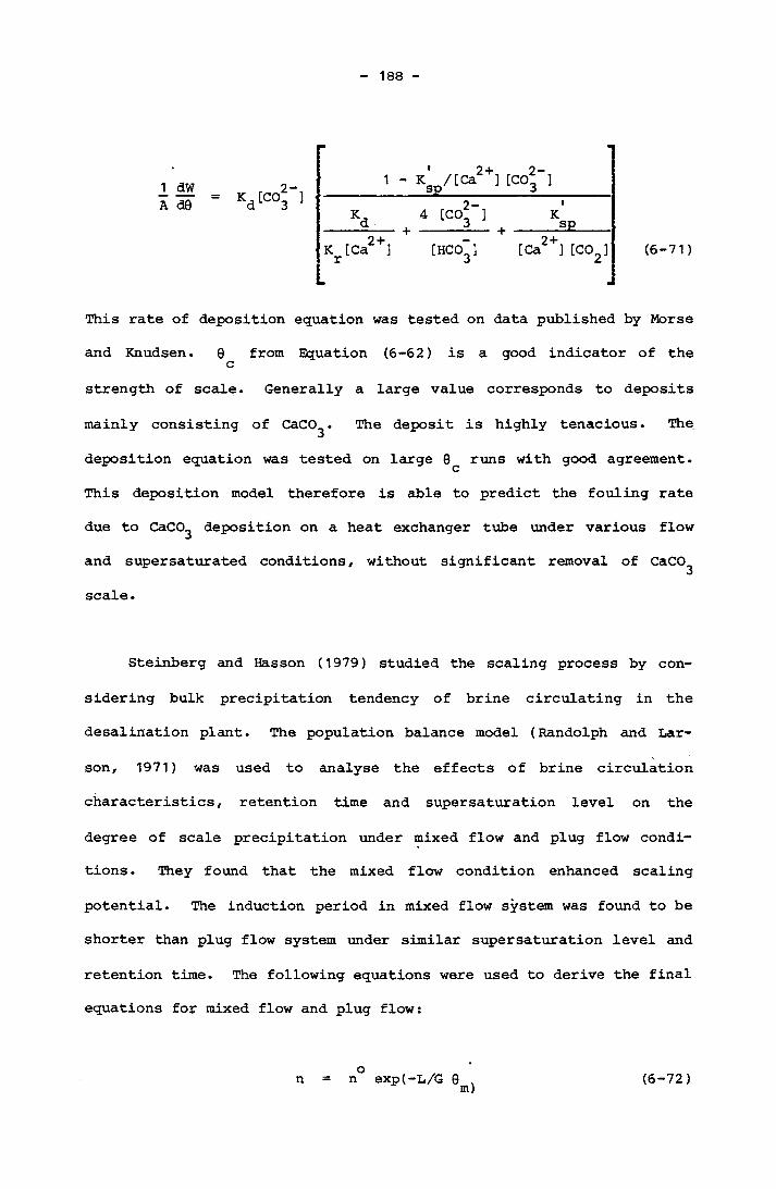
188
1 dwA d0 VC03_1
' 2 + 2-1 - K /[Ca ][C0_ ] _____ Sp ___ 3
2 +K [Ca2 ] r
4 tCCL_]+ --------- +
[HCO~] [Ca2+][C02] (6-71)
This rate of deposition equation was tested on data published by Morse
and Knudsen. 0 from Equation (6-62) is a good indicator of the cstrength of scale. Generally a large value corresponds to deposits
mainly consisting of CaCO^• The deposit is highly tenacious. The
deposition equation was tested on large 0^ runs with good agreement.
This deposition model therefore is able to predict the fouling rate
due to CaCO^ deposition on a heat exchanger tube under various flow
and supersaturated conditions/ without significant removal of CaCO^
scale.
Steinberg and Hasson (1979) studied the scaling process by con
sidering bulk precipitation tendency of brine circulating in the
desalination plant. The population balance model (Randolph and Lar
son, 1971) was used to analyse the effects of brine circulation
characteristics, retention time and supersaturation level on the
degree of scale precipitation under mixed flow and plug flow condi
tions. They found that the mixed flow condition enhanced scaling
potential. The induction period in mixed flow system was found to be
shorter than plug flow system under similar supersaturation level and
retention time. The following equations were used to derive the final
equations for mixed flow and plug flow:
on = n exp(-L/G 0 4 (6-72)m)
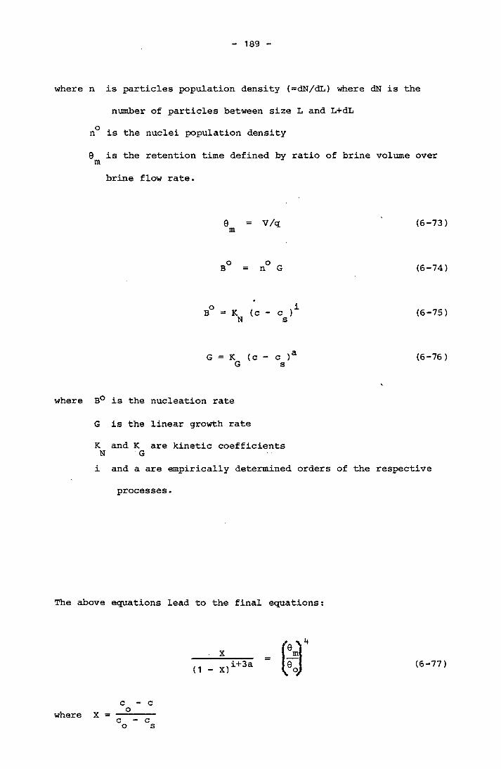
189
where n is particles population density (=dN/dL) where dN is the
number of particles between size L and L+dL
n° is the nuclei population density
9 is the retention time defined by ratio of brine volume over mbrine flow rate.
9m V/q
oB (c - C )s
G = K (c - c )a G s
(6-73)
(6-74)
(6-75)
(6-76)
where B° is the nucleation rate
G is the linear growth rate
K and K are kinetic coefficients N Gi and a are empirically determined orders of the respective
processes.
The above equations lead to the final equations:
(1
XX) i+3a (6-77)
c - coc - c o s
where X
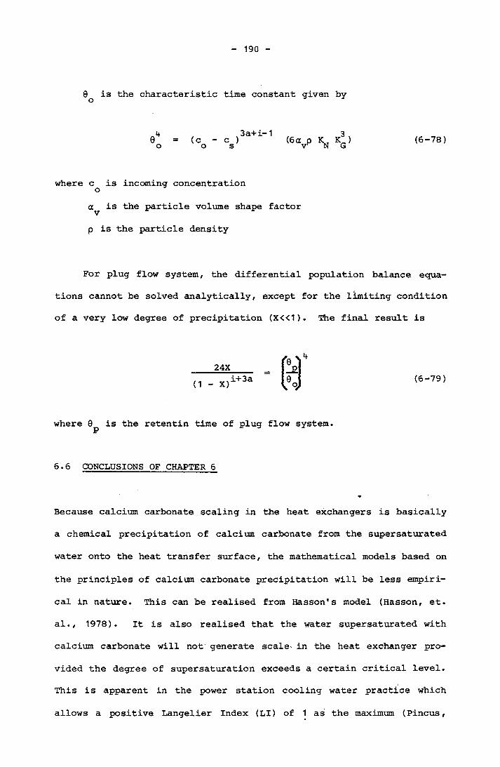
190
9 is the characteristic time constant given byo
4 3a+i-1e = (c - c ) (6-78)o o s
where c is incoming concentrationoa is the particle volume shape factor
p is the particle density
For plug flow system, the differential population balance equa
tions cannot be solved analytically, except for the limiting condition
of a very low degree of precipitation (X<<1)• The final result is
where 9^ is the retentin time of plug flow system.
6.6 CONCLUSIONS OF CHAPTER 6
Because calcium carbonate scaling in the heat exchangers is basically
a chemical precipitation of calcium carbonate from the supersaturated
water onto the heat transfer surface, the mathematical models based on
the principles of calcium carbonate precipitation will be less empiri
cal in nature. This can be realised from Hasson's model (Hasson, et.
al., 1978). It is also realised that the water supersaturated with
calcium carbonate will not generate scale in the heat exchanger pro
vided the degree of supersaturation exceeds a certain critical level.
This is apparent in the power station cooling water practice which
allows a positive Langelier Index (LI) of 1 as the maximum (Pincus,
(1 - X)24X
i+3a (6-79)

191
1962). To test the validity of this practice and also the roles of
other factors when using Langelier Index to monitor the quality of the
cooling water for the scale-free operation of the power station cool
ing water system, the following chapter is devoted in setting up the
pilot scale experiment on Lake Liddell power station cooling water.

192
CHAPTER 7
INVESTIGATION OF SCALING POTENTIAL OF LAKE LIDDELL WATER
TO POWER STATION CONDENSER TUBES
7.1 INTRODUCTION
Lake Liddell Power Station is one of the largest power stations
installed by the NSW Electricity Commission. This base load station consists of four sets of 500 MW generators and is able to generate
200 0 MW of electricity at full capacity. Each set of water cooling
condensers used with a 500 MW generating set is one of the world's
largest mass and heat transfer devices. It condenses steam from the
turbine exhaust at low pressure and hence at low temperature, which
ensures that the maximum amount of heat is extracted from the steam. The source of cooling water is an artificial cooling pond next to the
station with an area of 1100 hectares. The water is circulating
continously through the condenser tubes and back to one pond to
dissipate heat. Water lost through evaporative cooling is replaced by
natural inflow and by pumping from the nearby Hunter River. An
investigation had been carried out to determine the scaling potential
of Lake Liddell water to power station condenser tubes. The power
station at the time of investigation was operated at positive
Langelier Index (LI) of +1 as the maximum, which complied with the
usual cooling water practice (Pincus, 1962). This was achieved by
controlling the methyl orange alkalinity (total alkalinity) of the
lake by dosing sulphuric acid. Owing to the size of the pond, the

193
sulphuric acid dosage required to control M.O. alkalinity is enormous. For example, it requires 4,670 tonnes of sulphuric acid to reduce the lake M.O. alkalnity from 130 p.p.m. to 100 p.p.m. The water quality during the time of investigation is given in Table (7-
1).
TABLE 7-1 Data of Lake Liddell Water for 1979-1980
M.O. ALkalinity (mg/L CaCO^)
Range
97-134
Typical
118Ca hardness (mg/L CaCO^) 174-260 206Total hardness (mg/L CaCO^) 396-494 436
Sulphate (mg/L S04) 250-460 349
Chloride (mg/L Cl”) 120-216 184
pH 7.7-9.1 8.2
Conductivity ((is/m) x 100 1270-1690 1370
Since Langelier Index (LI) was used to monitor the scaling potential
of the lake water, the investigation was to determine experimentally the margins of reliability of the Langelier Index for scaling control
of the condensing system. The requirement of sulphuric acid dosage could be calculated accordingly. This investigation was carried out by a test rig constructed to simulate the Lake Liddell power station
condensing system as described in the next section. It was intended
that these results would provide minimum sulphuric acid addition to Lake Liddell and hence minimum sulphate addition to the Hunter River
without adverse effects on power generation due to loss of thermal conductivity.
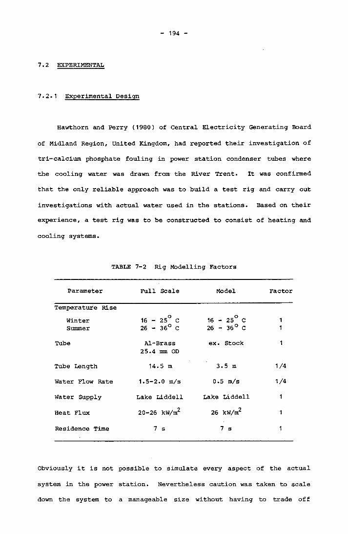
194
7.2 EXPERIMENTAL
7.2.1 Experimental Design
Hawthorn and Perry (1980) of Central Electricity Generating Board
of Midland Region, United Kingdom, had reported their investigation of
tri-calcium phosphate fouling in power station condenser tubes where
the cooling water was drawn from the River Trent. It was confirmed
that the only reliable approach was to build a test rig and carry out
investigations with actual water used in the stations. Based on their experience, a test rig was to be constructed to consist of heating and
cooling systems.
TABLE 7-2 Rig Modelling Factors
Parameter Full Scale Model Factor
Temperature RiseWinter o16-25 C 16 - 25° C 1Summer 26 - 36° C 26 - 36° C 1
Tube Al-Brass ex. Stock 1
Tube Length25.4 mm OD
14.5 m 3.5 m 1/4
Water Flow Rate 1.5-2.0 m/s 0.5 m/s 1/4
Water Supply Lake Liddell Lake Liddell 1
Heat Flux 20-26 kW/m2 26 kW/m2 1
Residence Time 7 s 7 s 1
Obviously it is not possible to simulate every aspect of the actual
system in the power station. Nevertheless caution was taken to scale
down the system to a manageable size without having to trade off
195
features that are important to scaling. The test rig was scaled down
according to Table (7-2).
The velocity of the cooling water flow was reduced to 25% of the
original flow rate in order to maintain the residence time, heat flux and temperature rise as in the actual plant. Fortunately, this
velocity still falls into the region of turbulent flow as required for
convective heat transfer in a heat exchanger. The slower velocity is
thought to be more conducive for scale growth because of lower velocity shear stress on the tube wall. The rig is shown
schematically in Figure (7-1).
7.2.2 Experimental Apparatus
7.2.2.1 Heating System
Instead of the low pressure condensing system in the power
station, hot water was used as the heating medium to achieve a similar
heat flux. A 4m length 1" 18 gauge Aluminium Brass condenser tube
supplied by the Electricity Commission of New South Wales was surrounded by a hot water jacket with hot water recycled continuously
from a 200 litre galvanized drum equipped with 2x4 kW heaters. The
heaters were single phase stainless steel grade 316 Birko immersion
heat (Birko-Electric (Sales) Pty Ltd, Australia). The hot water
jacket was a 3.55 m length 200 mm nominal diameter asbestos cement
pipe with both ends enclosed. The asbestos cement pipe was supplied by James Hardie and Coy Pty Ltd. The condenser tube was placed in the
hot water jacket and secured by pressure fittings on both ends. The
pressure fittings were brass hexagonal caps with 1" BSP female thread

TO MANOMETER195a
FIGURE 7-1 Schematic Representation of Test Rig
196
that screwed into a 1" BSP male brass plain nipple with the other end
screwed into a 2" brass bush. An O-ring was placed between the
hexagonal cap and plan nipple to secure a tight seal. A 1" opening on
the hexagonal cap was available for the tube to move through the hot
water jacket. Two Gibault fittings designed by the supplier, James
Hardie and Coy Pty Ltd were used for both ends of the asbestos cement pipe. The fitting had a 2" BSP tapping to receive the pressure
fitting. The whole arrangement made up the hot water jacket and was
completely sealed at both ends of the pipe by the O-ring in the
hexagonal cap tightened onto the tube. A new condenser tube was used
for each experiment. Therefore with this arrangement, the hexagonal
cap could be simply unscrewed and the tube removed from the hot water jacket. A drawing is shown in Figure (7-2).
The hot water was pumped into the jacket by a 3/4 hp single phase
Volu-flo closed coupled centrifugal pump (Scruttons Pty Ltd,
Australia) via 6 hot water regulating valves equally spaced apart.
These hot water regulating valves were 1/2" Whitey regulating and shut-off valves (Sydney Valve and Fitting Pty Ltd, Australia) that
allowed a precise flow rate to be regulated. The pressure drop across
each valve measured by the water manometers was adjusted to achieve
similar flow rates into the jacket. Therefore, a fairly uniform bulk
temperature of the hot water in the jacket was possible. The bulk
temperature of the hot water in the jacket was measured by a Pt10 0element 3 wire lead resistance thermometer with 0.01% accuracy
supplied by Richard Foot Pty Ltd, Australia. The hot water was pumped
at the flow rate of 32 litres per minute at 58° C. The flow rate was measured by a Brass IGU Gapmeter with the measurement range 8-80 L/min
(supplied by Duff and Macintosh Pty Ltd, Australia). The temperature
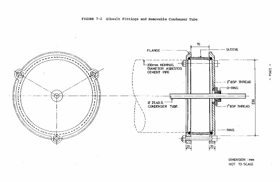
FIGURE 7-2 Gibault Fittings and Removable Condenser Tube196a
V/V
/V S////7
-> LU
DIMENSION : mrr NOT TO SCALE

197
of the hot water was controlled by the temperature controlling unit comprising a West Guardian Q3X temperature controller with scale and calibration 0 to 100° C equipped with proportional, integral and
derivative controlled function, a single phase 240 volts thyristor with maximum power of 16,000 watts and a special tolerance
copper/constantant thermocuple for the temperature feedback. All these items were supplied by Richard Foot Pty Ltd, Australia. The resulting bulk temperature in the jacket was approximately 55° C. The
designed heat flux was achieved when the inlet water was set for summer conditions. A 70 mm immersion mercury thermometer with 0.1° C resolution was installed at both ends of the tube with the thermometer bulb inserted in the flowing water to measure the inlet and the outlet temperatures. The whole heat system was insulated with 1" thick Rockwool insulator supplied by Bestobell Engineering Products. Alfloc 2000 from Catoleum was added to the hot water to serve as a corrosion
and scaling control reagent.
7.2.2.2 Cooling System
The cooling system is to cool down the water after passing
through the condenser tube and hence maintain the inlet water temperature constant. At the same time the cooling system has to simulate Lake Liddell used as the cooling pond which serves the Liddell power station. In view of these, an above-ground pool with
4.5 m total volume and 7.3 m total surface area supplied by Clark Rubber Ltd, Australia was installed to dissipate the majority of the
heat. The rest of the heat was dissipated by a simple coil-type heat exchanger consisting of a 26 m length 1/2" 19 gauge helical coppercoil packed in a 1.5 m tall 200 mm I.D. perspex column. The warm
198
lake water was fed into the bottom of the perspex column, rose up to the top and overflowed into the above-ground pool. A single-passed of tap water was used as the coolant. As a result there was no control
over fluctuations of ambient temperature and tap water temperature.
Nevertheless, the combination of above ground pool and coil-type heat exchanger was able to maintain the inlet water temperature for summer
conditions to within 3°C. The Lake Liddell water was pumped continuously at the flow rate of 12 L/min by a 1/4 hp single phase all bronze Volu-flow closed coupled centrifugal pump supplied by Scruttons
Pty Ltd, Australia. The flow rate was measured by a rotameter (Precision Bore Florimeter Tube No. FP-3/4-27-G-10/83 supplied by F & P Pty Ltd, Australia).
7.2.3 Experimental Procedure
The cooling water (Lake Liddell water) tested in the rig was pumped continuously at the flow rate of 12 L/min, which gave rise to
the flow velocity of 0.5 m/s in the condenser tube. A rise of 8° C of the water when leaving the condenser tube was observed for a 2 5° C inlet water temperature throughout the experiment. The inlet and outlet temperatures of the water were constantly measured by the mercury thermometer of 0.1° C resolution at each end of the tube. The
bulk temperature in the hot water jacket measured by resistance thermometer, the overall heat transfer coefficient of the unit was
calculated. The reduction in overall heat transfer coefficient based on outside diameter of the tube serves as an indication of fouling. The chemistry of the water was constantly monitored by measuring pH,
M.O. alkalinity, Ca hardness, Mg hardness, sulphate and chloride
concentrations. Ca and Mg hardness were determined according to the

199
method given by Diehl et. al. ( 1950). The rest of the species were
analysed according to Standard Methods (Standard Methods for the
Examination of Water and Wastewater, 1980). Conclusion of each
experiment was only made after the cooling water (lake water) had been
pumped continuously for more than 100 hours.
The experiment was carried out in three stages.
Stage 1: Summer condition synthetic water experiment, with totalalkalinity as the variable.
Stage 2: Summer condition Lake Liddell water experiment, with total
alkalinity as the variable.Stage 3: Summer condition Lake Liddell water experiment, with Ca
hardness as the variable.
The chemical composition of each experiment was adjusted by dosing an
appropriate quantity of technical grade CaCl2, MgCl2, NaHCO-j and
Na2SO^. pH adjustment was done by dosing sodium hydroxide. A new
condenser tube was used for each experiment.
The chemicals and the quantity used for synthetic water to
simulate typical lake water chemical composition are shown in Table
(7-3).

200
3TABLE 7-3 Chemicals Used for 4.5 m Synthetic Water
Chemical Weight Typical Lake
(kg) Water Composition
CaCl^ (fused) 1.50 Ca hardness - 206 mg/L CaCO^
MgCl2 1.00 Mg hardness - 230 mg/L CaC03
Na2S04 2.30 Sodium - 127 mg/L Na+
Sulphate - 349 mg/L SO^
Chloride - 184 mg/L Cl
NaHC03 0.91 M.O. alkalinity 118 mg/L CaCO^
RESULTS AND DISCUSSION
Methyl Orange Alkalinity Experiments
These are the experiments carried out at stage 1 and stage 2 on
the rig using both synthetic and actual lake water with methyl orange alkalinity varied by dosing sodium bicarbonate to investigate the
scale-forming tendency in the condenser tube.
A total of nine experiments were carried out, of which the first
four experiments were with synthetic water which was prepared to
simulate lake water by adding chemicals to tap water. Experiments 5,
6, 7, 8 and 11 were with lake water transported from Lake Liddell and
deliberately dosed with sodium bicarbonate to specific methyl orange
alkalinities. Results are tabulated in Tables (7-4) and (7-5).
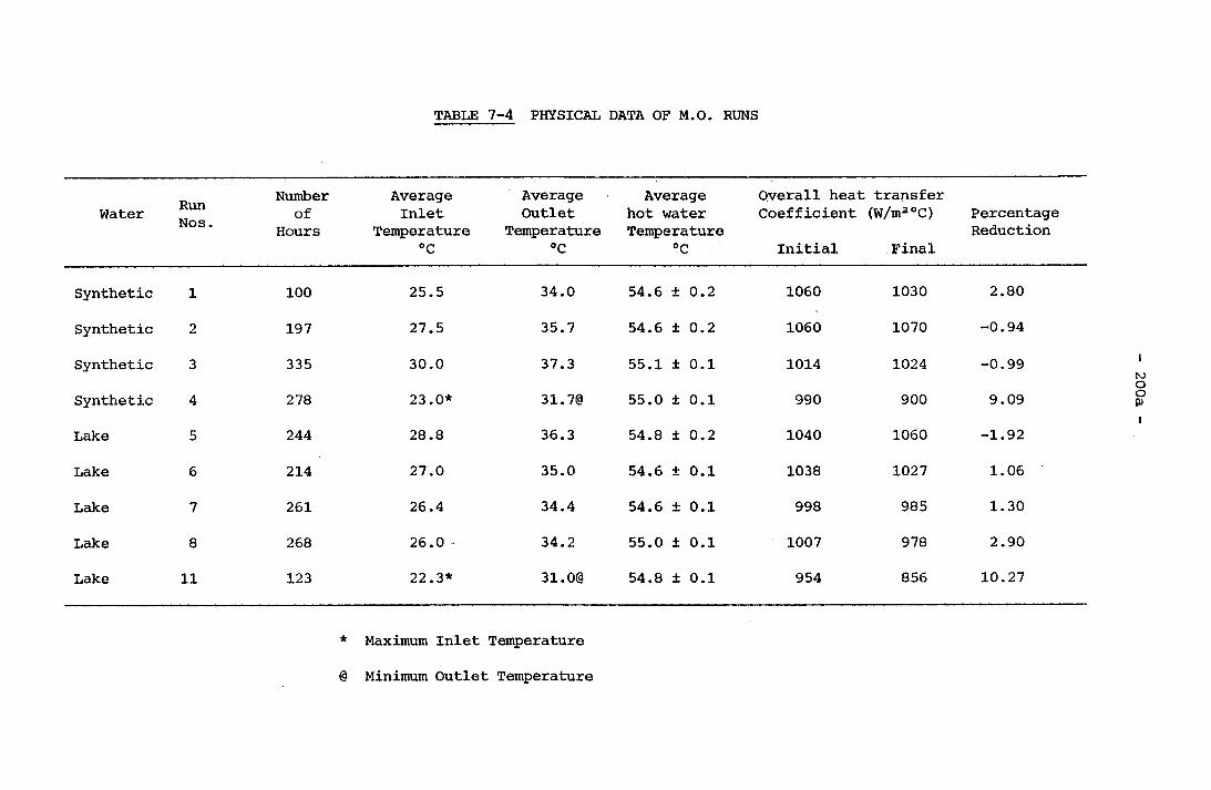
TABLE 7 -4 PHYSICAL DATA OF M.O. RUNS2
00
a
d)Cn G
td
0
O
p1
00 cn
cn
OI
<n<T>
OI
cnocn
CNcnrHI
COOrH
OnorH
OcnCN
r-CNorH
po
—
4H
U
cn o
C
Ntd
ep \
-p
^
-pCtJ<U42
rHtdG•rHpHrHtd•rH-P•rHGPt
O
Oco
r-
o o
rH
rH
-d*CNOrH
OocnocoorH
r-CNorH
incocn
ooe'en
COunco
o o
vO vO
o o
rH
rH
P1
rHOrH
Ocncn
oorH
00COOr-H
00cncnr-oorH
incn
d)pG-Ptdpa)i4
a)EH
CN CN
rH
O
O
O
+1 HH
+1
VO
vO
rHmm
in
in
rH
CN rH
o o
o+1
+1 +1
O
00 VO
inin in
in
rH
rH
rH
O
O
O
+1 -H
-H
VO
O
00
inin
m m
a)tn -P td
a) a)pG-PcdP<Di4
0)
o
r-inCO
CO
COr-co
CSIr-rHCO
COvOCO
oincoco
©c
n o
^
rHCO
co
d)
diCn -Pid
<u
d)pG-Ptdpd)|<uEi
in m
in r-
CN CN
ooco
HeOCOCN
CO00CN
or-CNVOCN
OvOCN
HeCOCNCN
P<D$GS
cnm
h p
0
G
0
tC
o
ino
cn
corH
rH
CO
00r-CNCN
'd'
rHCN
rHVOCN
COvOCN
COCNrH
He ©
G
cnG
0H
CN CO
rr m
VO
CO rHrH
pdJ•pcds
u•H-pd)42-pG>
.CO
a•H-pdJH->G>1CO
o■H-p<v■5G>1CO
o•rH-pd)42-pG>1CO
d)44cdPI
<1)<dPI
cu a>
cu44
44 44
cd td
cdPI
PI PI
Maximum Inlet Temperature

TABLE 7-5 CHEMICAL DATA OF M.O. RUNS
200b
on•HuorHs:ua; nr
■p o <d wrdft H-] rH \3
cn cn g
mwa)dTJHfdftcnSuiU)a)dT)ucdftnju>1-p•Hd■HrHrdrH<
S’S’S'xft
iH03d•HftrH03•H-p•HdHi—I03d•Hft<H03•H-P•HdHrH03d•HftrH03-p■HdHiH03d•HftI—I03•H-P•HdHi—I03d•HftrH03•H-P•HdHiH03d•Hfti—I03•H'-P•HdH
d w d o ft z
inCMrH
nTCOrH
OCNrH
LO nT
m o
rH rH
OOin
CnnTmovorHcninrHinmCMnTmCM
nTcn
oinnrme'en
mvorH00inrHr-mCMVOmCM
o o
m
cmrH
rH
H
<T>nT
OrH
rH
nr cn
CO nT
rH cn
CM VO
H1 cn
CM nT
CO nT
O
rHCM
CMCOCMCM
nT nj<
O0^0
0
rH cm
cn
oCM
OCMcnrH
OnrrHcn
nTrHcn00CMinrHCM00rH
COVOCMVOnTCMCOCOinrHCOnTcnocnomCMcnCMvovoCMocnrHOCMrHrHrHOcn
cncnCMVOvoCMinCMVOrHcnincnocnvoCMCMomoCOCMCMOCMincncnrH
00CMcncncnCMcnvovoinCMvonrnrcnco<nCMrHcncncnrHcnCMvocn
o
nrcn
cmrH
cnCMmCMnr
t"mcnoCMcninCMr-omvoCMcncncnCMcnoincncocncnr-oinoconrr"mmrH
VOnrnrcnrHrH 1016 869 241 49 279 288 450 475 290 306
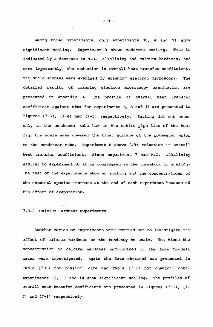
201
Among these experiments, only experiments 10, 4 and 11 show
significant scaling. Experiment 8 shows moderate scaling. This is indicated by a decrease in M.O. alkalinity and calcium hardness, and
more importantly, the reduction in overall heat transfer coefficient.
The scale samples were examined by scanning electron microscopy. The
detailed results of scanning electron microscopy examination are
presented in Appendix E. The profile of overall heat transfer
coefficient against time for experiments 4, 8 and 11 are presented in
Figures (7-3), (7-4) and (7-5) respectively. Scaling did not occur
only in the condenser tube but in the entire pipe line of the test
rig; the scale even covered the float surface of the rotameter prior
to the condenser tube. Experiment 8 shows 2.9% reduction in overall
heat transfer coefficient. Since experiment 7 has M.O. alkalinity
similar to experiment 8, it is considered as the threshold of scaling. The rest of the experiments show no scaling and the concentrations of
the chemical species increase at the end of each experiment because of
the effect of evaporation.
7.3.2 Calcium Hardness Experiments
Another series of experiments were carried out to investigate the
effect of calcium hardness on the tendency to scale. Ten times the
concentration of calcium hardness encountered in the Lake Liddell
water were investigated. Again the data obtained are presented in
Table (7-6) for physical data and Table (7-7) for chemical data.
Experiments 12, 13 and 14 show significant scaling. The profiles ofoverall heat transfer coefficient are presented in Figures (7-6), (7-
7) and (7-8) respectively.

00 • l
201aO
oo o
o © ©
o
o§
o&© oo
I 1
1cno
ocr>6
i/joo_Ce
oo
-* oa06
3 u
u/)u
d i d i ^
90D
jajsu
oj}
iid-O
aq
z
FIGURE 7-3 Change of Overall Heat Transfer Coefficient with Time, Expt.

201b
© O
o
o O
3o
^uj / av^ lu
aio
iy^
OD
j3^S
ud
j4. ;D
9i|
11DJ9A
Q
00FIGURE 7-4 Change of Overall Heat Transfer Coefficient with Time, Expt.
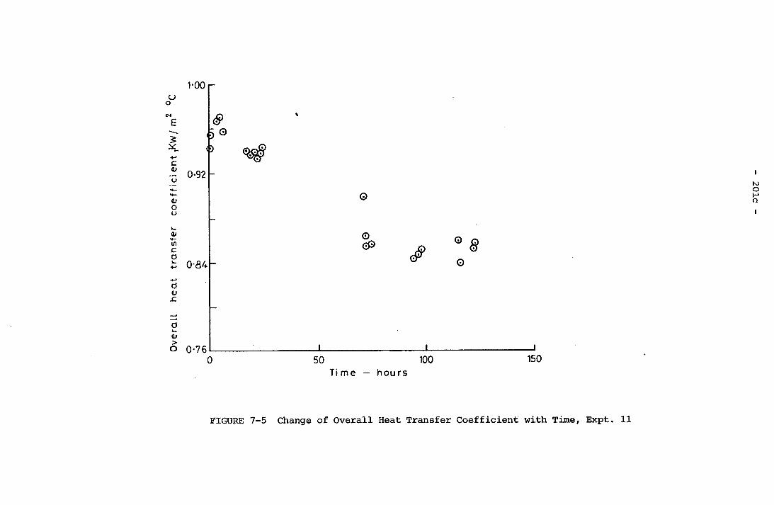
1-00
201c
o
I%
QCMcn6
3 uu /
m^1 iu
a |d| uaoD
jajsuD
n
ntuaAO
0 z
FIGURE 7-5 Change of Overall Heat Transfer Coefficient with Time, Expt. 11

1-08201d
eaacaa.oCOCO
^4-c
4-
(Ja-SC
o -
o2
8°
% P0 ©
I O)0 i
ooCMOo
30-C1CD£i—
Mfqoo
liDcnCMCTio
3q ^uu/M^n 4,u3p!^aoD ja^suDj;
4-Daq i]Djsaq
FIGURE 7-6 Change of Overall Heat Transfer Coefficient with Time, Expt. 12
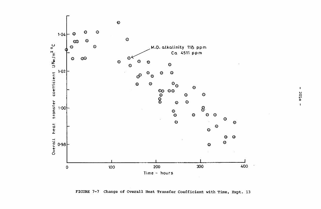
M.O. a lk a lin ity 116 ppm
201e
OOo
o8§o
oCMo
ooa3<T>6
3o2UU//V^n
;U3P!430D J 0 J.S UDJ 1
;t>aq V)D J 9 AQ
FIGURE 7-7 Change of Overall Heat Transfer Coefficient with Time, Expt. 13
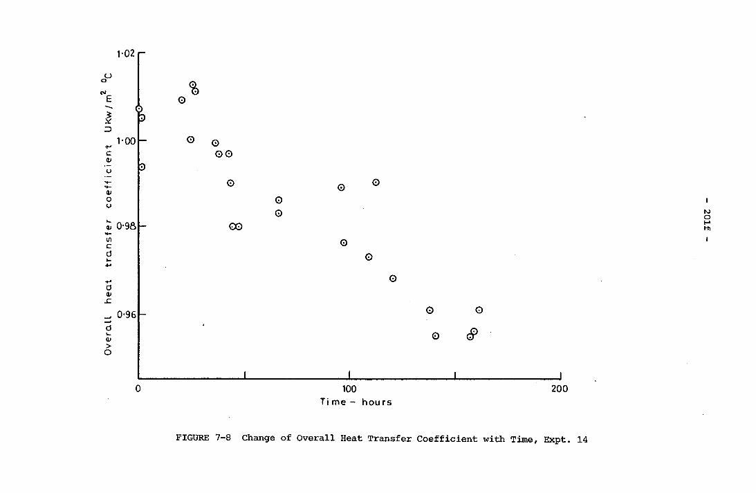
1-02201f
ooCSI
o%
O©
O
oo
o o
O 0
ePo
o o
0®
o
8
ooCO<T>6
U3
<T>6
'0 z uu / m
x n ;u
aiDiy
aoD
ja^su
Di;
loaq
y| d ja AQ
FIGURE 7-8 Change o f O v e ra l l H eat T r a n s f e r C o e f f i c i e n t w ith T im e, E x p t. 14

20
1g
c/3§05COCOwCmO<C§Q
03O'
Gtd
0-P
-HG
-Pr-
voCN
CN03
o•
••
•o
pp
ino
P
T3p
1<u
a)CU
05
u03 —
pP
CJ(d
pin
CNai
oG
coCO
inO
'G a
PO
'O
'O
'O
'a
£CP
p \
-p is>—*
■prd P
a) c
X
a)•H
PrH
Otd
r-H P
pp
r-o
fO P
PLD
cno
O'
P
<Pp
oo
oO
'a)
a)G
pp
p
>
oH
o o
0)Pp
pp
pd)
p
p•
••
•O
' a)
po
oo
ocd
P
idP
fO P
+1+1
+1+1
<u S
a)>
ft
VOin
VOvo
CP
S•
••
•o
03*3*
,C
Elin
inin
in
03co
p•
03 P
*He
Heo
O' P
P
CDVO
O'
f0 CD
fdO
••
•+
1P
rH
Po
COin
03 P
03co
coCO
CO>
p a
•< o
em
0)co
Eh0)po
in03
0•
••
•O
' P
PCN
oo
oro
a) td
UP P
Po
+1+1
+i
+i
a) g
a)>
h a
COCN
r-<
••
••
<uin
inin
mEH
CNCN
CNCN
P03 03
P P
PCN
vop
CNe
o
or-~
e'vO
3
0p
enP
pZ
ffi
G
03CN
COm
3
OP
pP
p
05 Z
P0)Prd50)
0303
03X
XX
Xrd
tdro
PP
pP
c203Xppo<upPrd0)i1<upprH<ui—
i-pPop0303XO
'•HX03XE-t
He
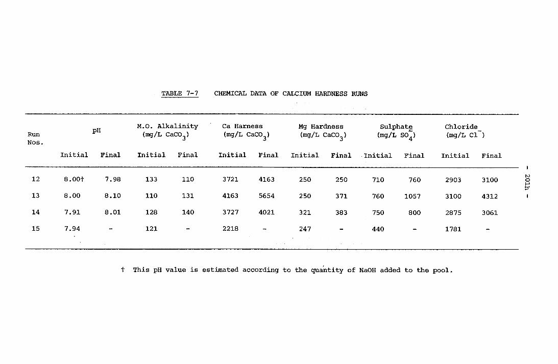
201h
§maw1aDH3CmO<<QPICOHar-ia9Eh
rHcdO
CNrH
Go
rHa
•HrH
COo
1a
aCO
CD rH
03 u
•HrH
P
P5cd
o \
•Ha
Oa
rHrH
tP-P
OO
p~a
g
e•H
CPrH
ap*
u
—G
CNCO
CNrH
HrHcdO
p*o
G<0
ino
1a)ii
^•H
oa
■P o
arH
cd in
Ga
pj
rH \
rHP a
cda j3
•Ho
Oo
o-P
rH0
in•H
p*p~
■'tfGHrH
*cd
orH
CO(0
aG
mP
'a
1CO
O•H
CNco
CO0)
CJa
G
cd03
UPcd
pj
rHa \
cda
•Ho
orH
r-a g
•Pin
inCN
a ~
•HCN
CNa
CNGHrHcd
arH
^—.
G0
inCN
a•H
rHID
O1
CO O
am
"3*co od)
cdc u
prH
id P3
cda \
•HrH
COIs*
aS
'-p
CNis
CNrH
id g
•Hr-
rHP»
au ~
Ga
aCN
H
>irH
-pcd
orH
o•H
GrH
CO1
G
a■H
rHrH
rH•H
Oa
rH
U(d
cdg u
rHrH
<
pi
cd\
•HCO
Oa
rH•
S'
-PCO
rHa
CNo
z•H
rHrH
rHrH
Ga "
HrH00
OrH
cdCP
rHO
G•
••
1■H
aa
aaa
rHcdH
-•H
Oo
rH'sP
-Po
oa
a-H
••
••
G0
0a
r**p*
H
G
toCN
COa
S3 0
rHrH
rHrH
a a
rHooa<urP■Po■p030)'a03cdSBocd2*wO>
i•P•P■P
. gcd<D
5O-P&>g•H03POoucda)-prdS•H-P(0a)co•HoGrH>aaCO•H.GEh
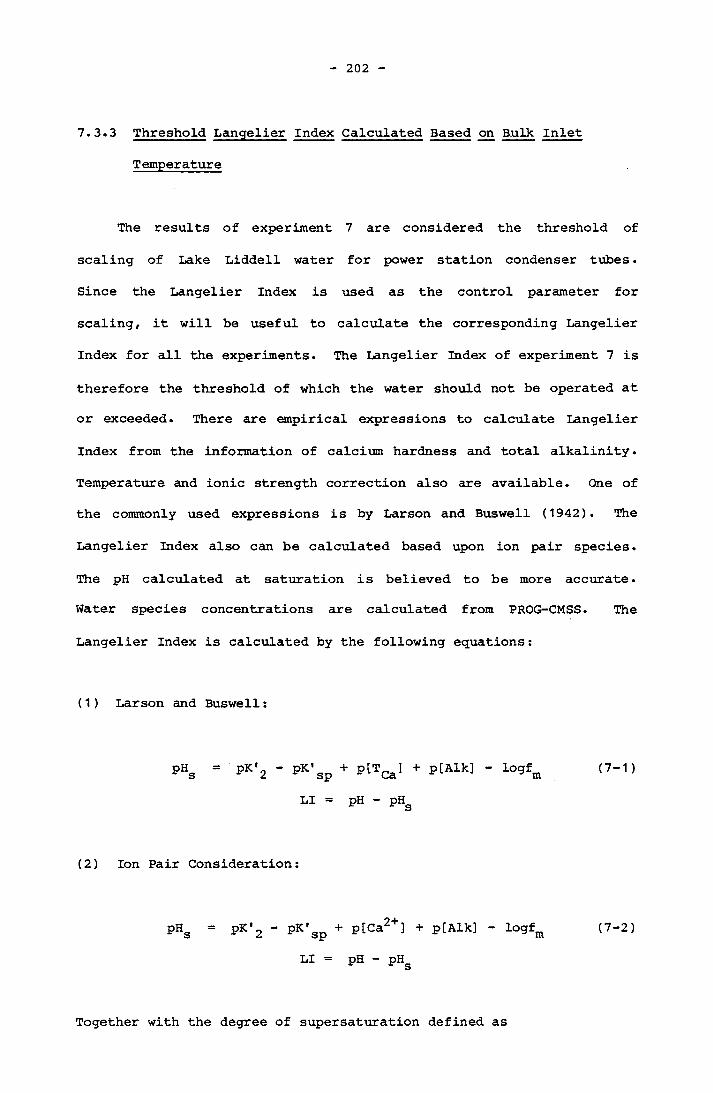
202
7.3.3 Threshold Langelier Index Calculated Based on Bulk Inlet
Temperature
The results of experiment 7 are considered the threshold of
scaling of Lake Liddell water for power station condenser tubes.
Since the Langelier Index is used as the control parameter for
scaling, it will be useful to calculate the corresponding Langelier
Index for all the experiments. The Langelier Index of experiment 7 is
therefore the threshold of which the water should not be operated at
or exceeded. There are empirical expressions to calculate Langelier
Index from the information of calcium hardness and total alkalinity.
Temperature and ionic strength correction also are available. One of
the commonly used expressions is by Larson and Buswell (1942). The
Langelier Index also can be calculated based upon ion pair species.
The pH calculated at saturation is believed to be more accurate.
Water species concentrations are calculated from PROG-CMSS. The
Langelier Index is calculated by the following equations:
(1) Larson and Buswell:
pHs = pK'2 - pK'sp + p[TCa) + p[Aik] - logfm (7-1 )
LI = pH - pHs
(2) Ion Pair Consideration:
pHg = pK'2 - PK'sp + p[Ca2+] + p[Alk] - lo9fm (7-2)
LI = pH - PHg
Together with the degree of supersaturation defined as
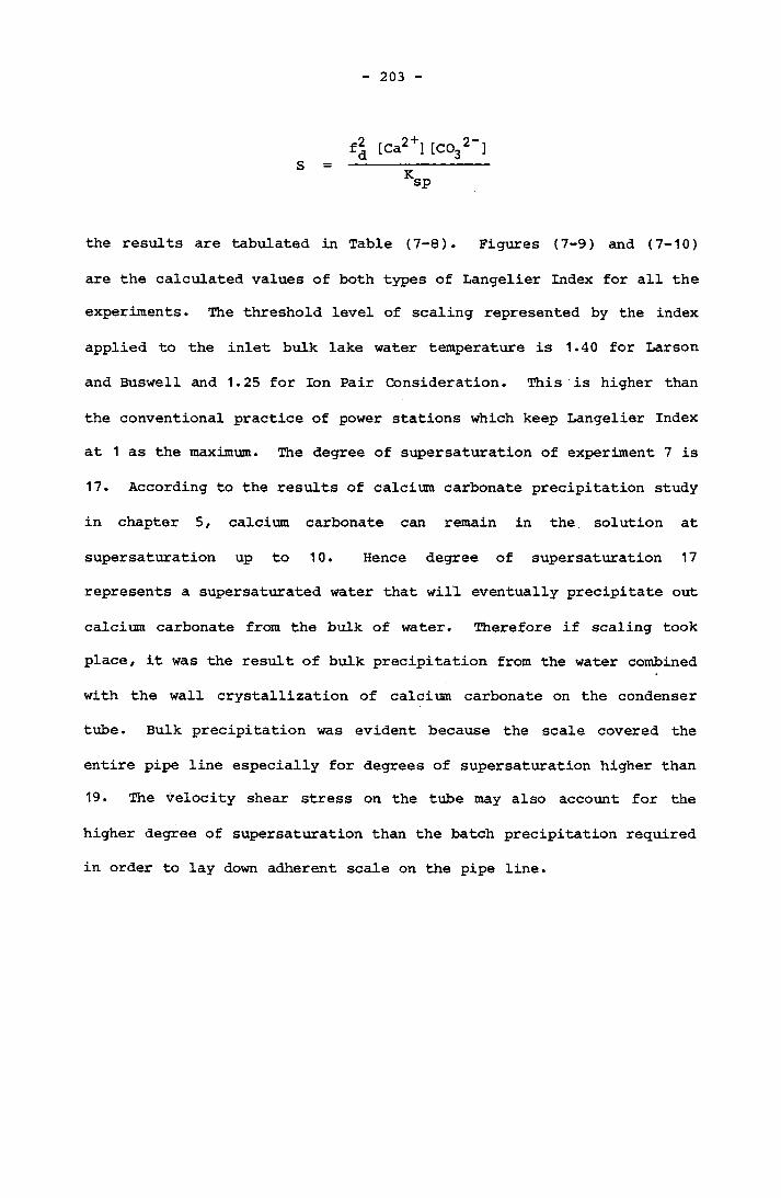
203
Sf| [Ca2+][C032"]
the results are tabulated in Table (7-8). Figures (7-9) and (7-10)
are the calculated values of both types of Langelier Index for all the experiments. The threshold level of scaling represented by the index
applied to the inlet bulk lake water temperature is 1.40 for Larson
and Buswell and 1.25 for Ion Pair Consideration. This is higher than
the conventional practice of power stations which keep Langelier Index
at 1 as the maximum. The degree of supersaturation of experiment 7 is
17. According to the results of calcium carbonate precipitation study
in chapter 5, calcium carbonate can remain in the solution at
supersaturation up to 10. Hence degree of supersaturation 17
represents a supersaturated water that will eventually precipitate out
calcium carbonate from the bulk of water. Therefore if scaling took
place, it was the result of bulk precipitation from the water combined
with the wall crystallization of calcium carbonate on the condenser
tube. Bulk precipitation was evident because the scale covered the
entire pipe line especially for degrees of supersaturation higher than 19. The velocity shear stress on the tube may also account for the
higher degree of supersaturation than the batch precipitation required
in order to lay down adherent scale on the pipe line.
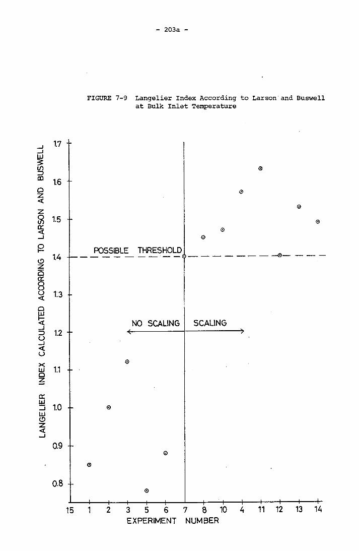
203a
FIGURE 7-9 Langelier Index According to Larson and Buswell at Bulk Inlet Temperature
in3coQz<z8cr<ozQcr8O<oLU
3O_J<oxLUQZcrLU
1.7 +
16 -
1.5 -
1.3 -
1.1 -
=5 1.0 -LUOz<
0.9 -
0.8 -
3 5 6 7 8 10EXPERIMENT NUMBER
11 12 13 14

203b
FIGURE 7-10 Langelier Index with Ion Pair Consideration at Bulk Inlet Temperature
15 -
1.4 -
13 -
2o1-2 -<crLUo
ldZoo 1.1 -
£zo
XLUQzcrLU_jLUOz<
1.0 --
0.9 -
08 --
07 --
POSSIBLE THRESHOLD
5 6 7 8 10 4EXPERIMENT NUMBER
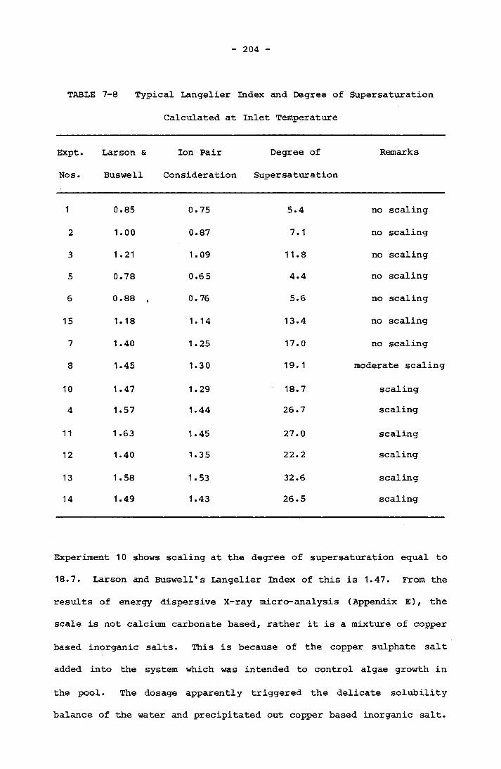
204
TABLE 7-8 Typical Langelier
Calculated at
Index and Degree of
Inlet Temperature
Supersaturation
Expt. Larson & Ion Pair Degree of Remarks
Nos. Buswell Consideration Supersaturation
1 0.85 0.75 5.4 no scaling
2 1.00 0.87 7.1 no scaling
3 1.21 1.09 11.8 no scaling
5 0.78 0.65 4.4 no scaling
6 0.88 . 0.76 5.6 no scaling
15 1.18 1.14 13.4 no scaling
7 1.40 1.25 17.0 no scaling
8 1.45 1.30 19. 1 moderate scaling
10 1.47 1.29 18.7 scaling4 1.57 1.44 26.7 scaling
11 1 .63 1.45 27.0 scaling12 1.40 1.35 22.2 scaling
13 1.58 1.53 32.6 scaling14 1.49 1.43 26.5 scaling
Experiment 10 shows scaling at the degree of supersaturation equal to
18.7. Larson and Buswell's Langelier Index of this is 1.47. From the
results of energy dispersive X-ray micro-analysis (Appendix E), the
scale is not calcium carbonate based, rather it is a mixture of copper
based inorganic salts. This is because of the copper sulphate salt
added into the system which was intended to control algae growth in
the pool. The dosage apparently triggered the delicate solubility
balance of the water and precipitated out copper based inorganic salt.
205
The salt subsequently deposited in the tube. It is probably a more
adherent scale than calcium carbonate scale because under similar flow
conditions, a thickness of 2-15 p,m was measured, whereas the scale
from experiment 8 was difficult to be measured.
7.3.4 Threshold Langelier Index Calculated Based on Heat Transfer
Surface Temperature
Calcium carbonate crystallization is surface reaction controlled as suggested by previous investigators and confirmed in Chapter 5. As
a result, the heat transfer surface temperature can be a critical
factor for scaling. The wall temperature can be estimated from the
water film heat transfer coefficient established in the tube under
fully turbulent flow (McCabe and Smith, 1967). An example to
calculate wall temperature at experiment 8 is shown as follows:
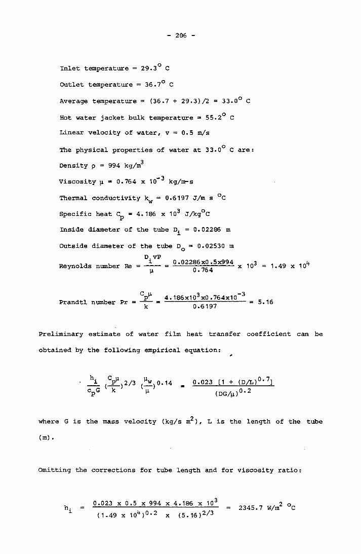
206
Inlet temperature = 29.3° C
Outlet temperature = 36.7° C
Average temperature = (36.7 + 29.3)/2 = 33.0
Hot water jacket bulk temperature = 55.2° C
Linear velocity of water, v = 0.5 m/s
The physical properties of water at 33.0° C
Density p = 994 kg/m3- 3Viscosity p, = 0.764 x 10 kg/m-s
Thermal conductivity k^ = 0.6197 J/m s °C
Specific heat C = 4.186 x 10³ J/kg°CJr
Inside diameter of the tube D. = 0.02286 miOutside diameter of the tube D = 0.02530 mo
D. vP„ , i 0.02286x0.5x994Reynolds number Re = ---- = -------—r—;------x pi 0.76 4
are :
x 103 1.49 x 10⁴
Prandtl number Pr 4.186x10³ xO .764x10 0.6197
5.16
Preliminary estimate of water film heat transfer coefficient can be
obtained by the following empirical equation:
hi {V\ 2/3 0.14 = 0.023 [1 + (D/L)0,7]
CPG k ^ (DG/pi)0 *2
2where G is the mass velocity (kg/s m ), L is the length of the tube
(m) .
Omitting the corrections for tube length and for viscosity ratio:
0.023 x 0.5 x 994 x 4.186 x 103 . 2 oh = ------- ----------- ------------------------- ---------- ----- = 2345.7 W/m °C(1 .49 x 104)°* 2 x (5.16)2/3

207
To determine wall temperature, the following equation can be used
ATDo/Dihi1/uo
AT
where AT^ is the temperature drop through inside fluid, °C
AT is the overall temperature drop, °C
U is the overall heat transfer coefficient based on outside odiameter, W/m2 °C
The overall temperature drop A T = 55.2 - 33.0 = 22.2°C
The surface area of the condenser tube based on outside diameter = 2 x
n x (0.02530/2) x 3.55 m = 0.282 m20.02286 2The heat input = 0.5 x 4.186 x (--- ---- )n x 994 x (36.7 - 29.3)
= 6.28 KW(55.2-29.3)-(55.2-36 .7)
The log mean temperature difference = ln [ (55.2-29.177155 .'2-36.7 )']2 OThe overall heat transfer coefficient = q/A A T = 1020 W/m C
The temperature drop over the water resistance:
AT 0.02530 x 10²⁰ 0.02286 x 2345.7 X (55.2-33) 10.7 °C
T , = T + AT. = 43.7°Cw 1
The viscosity of the water at T is now found:w
0.615 x 10⁻³ kg/m s
The viscosity-correction factors = 0.9701
The corrected coefficient h^ = 2275.5 W/m2 °C
The temperature drop over the water resistance and the wall

208
temperature become
ATi =0.02530x10²⁰ n
0.02286x2275.5 X (55'2-33) = H°C
Tw = 33+11 = 44°C
This is so close to the wall temperature calculated previously that a
second approximation is unnecessary.
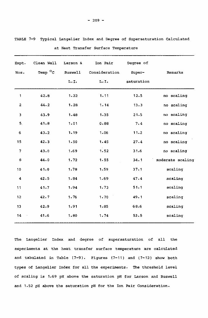
209
TABLE 7-9 Typical Langelier Index and Degree of Supersaturation Calculated
at Heat Transfer Surface Temperature
Expt.
Nos.
Clean Wall
Temp °C
Larson &
Buswell
L. I.
Ion Pair
Consideration
L. I.
Degree of
Super
saturation
Remarks
1 42.8 1.22 1.11 12.5 no scaling
2 44.2 1.28 1. 14 13.3 no scaling
3 43.9 1.48 1.35 21.5 no scaling5 41.8 1.01 0.88 7.4 no scaling
6 43.2 1.19 1.06 1 1.2 no scaling
15 42.3 1.50 1.45 27.4 no scaling
7 43.0 1.69 1.52 31.6 no scaling
8 44.0 1.72 1.55 34. 1 moderate scaling
10 41.0 1.78 1.59 37.1 scaling
4 42.5 1.84 1.69 47.4 scaling
1 1 41.7 1.94 1.73 51.1 scaling
12 42.7 1.76 1.70 49.1 scaling
13 42.9 1.91 1.85 6 8.6 scaling
14 41.6 1.80 1.74 53.5 scaling
The Langelier Index and degree of supersaturation of all the
experiments at the heat transfer surface temperature are calculated
and tabulated in Table (7-9). Figures (7-11) and (7-12) show both
types of Langelier Index for all the experiments. The threshold level
of scaling is 1.69 pH above the saturation pH for Larson and Buswell
and 1.52 pH above the saturation pH for the Ion Pair Consideration.
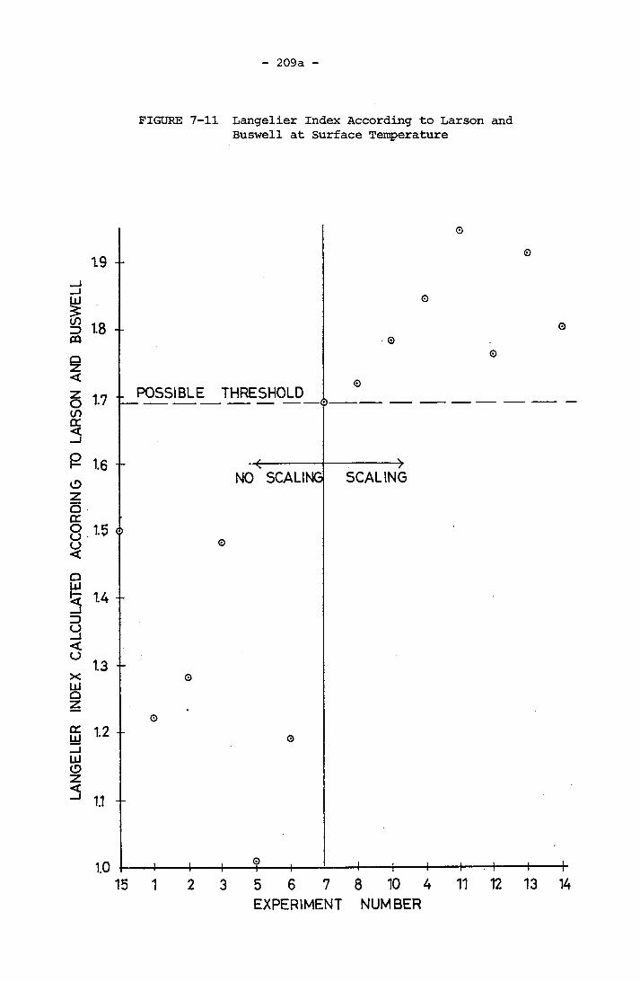
LAN
GE
LIER
INDE
X CALC
ULA
TED
ACCO
RD
ING
TO LA
RSO
N AN
D BU
SWE
LL209a
FIGURE 7-11 Langelier Index According to Larson and Buswell at Surface Temperature
1.7 - POSSIBLE THRESHOLD
©
©
©©
©©
©
^-------- ---------->NO SCALING
i
SCALING
©
G
o0
——--- 1 . - \ ■ ■—-?——i—— ■4----+-—4— I l < H-15 1 2 3 5 6 7 8 10 4 11 12 13 14
EXPERIMENT NUMBER

LANG
ELIE
R IN
DEX WI
TH I
ON P
AIR CO
NSID
ERAT
ION
209b
FIGURE 7-12 Langelier Index with Ion Pair Consideration at Surface Temperature
1.8 -
1.7 -
1.6 -
- 0 ©©©
©
POSSIBLE THRESHOLD©
_ _ _ _ _ _ _ _ _ _ _ _ _ _ _ _ _ _ _ _ _ _ _ _ _ _ _ _ _ _ XCj) \- - - - - - - - - - - - - - - - - - - -
NO SCALING SCALING
o
©®
©
©- - - - - - -4- - - - -I- - - - - - - - 1- - - - - —1- - - - - - - - - - - - - - - - - - - - - - - 1 1 1 1 \ —4-- - - - - - -
15 1 2 3 5 6 7 8 10 4EXPERIMENT NUMBER
11 12 13 14
210
Feitler (1972, 1974, 1975) introduced the concept of critical pH
which says that the precipitation from supersaturated solution will only happen at the pH which is exceeding the metastable limit
represented by critical pH. The saturation pH described the condition
of equilibrium between calcium carbonate solid and the ionic species.
This is the boundary line that divides the metastable and the unstable
region. It is known that calcium carbonate will not precipitate below
a certain degree of supersaturation without the presence of calcium
carbonate crystals. In fact this degree of supersaturaion is 10 as
found in unseeded batch precipitation experiment of calcium carbonate
described in Chapter 5. This means that there is a metastable region
for calcium carbonate solubility. Feitler felt that critical pH is a
more realistic index to predict the scaling tendency of the water.
This critical pH is determined by adding incremental quantities of NaOH to the CaCO^ water until the first sign of precipitation is
detected by the pH scaling meter designed by himself. The
corresponding pH is the initial pH which he believes is the boundary
of the metastable region and the labile region. Experiments had been
carried out by Feitler at 49° C for a range of calcium hardness and
total alkalinity. Feitler reported that the critical pH is 1.7 to 2.0
pH units above pHg. It is interesting to realise that 49° C is close
to heat transfer surface temperature of the test rig condenser tube,
which is also close to the actual Liddell Power station condenser. This piece of information therefore supports the reliability of the
present findings. Obviously this is only applicable to heat transfer
surface temperature consideration and should not be confused with the
inlet cooling water Langelier Index.
211
Experiment 12 is an interesting run. This is the only experiment
that shows scaling only in the condenser tube. Referring to Table
(7-9), Langelier Index calculated for experiment 12 at bulk water
temperature is 1.40 of Larson and Buswell and 1.35 of ion pair
consideration. According to this number, scaling should not take
place in the condenser tube. However, 1.76 and 1.70 for both types of
Langelier Index are obtained at the heat transfer surface. This has
exceeded the threshold Langelier Index, 1.69 and 1.52 represented by
experiment 7. The result is significant scaling, due to wallcrystallization rather than bulk precipitation as observed in
experiment 12.
7.4 CONCLUSIONS
The test rig investigation of scaling potential of the Lake
Liddell water to power station condenser tubes provides information to
be related to the actual performance of the Liddell power station
cooling water system. The normal operating Langelier Index at +1
recommended for cooling water practice (Pincus, 1962) without causing
scaling in the condenser tubes is considered valid, in fact it is
still conservative compared to the threshold Langelier Index found by
this investigation. The threshold Langelier Index also has to be
calculated based on the heat transfer surface temperature in addition
to the bulk inlet temperature because the heat transfer and surface temperature was found to be a critical factor for scaling. It would
be valuable to check the validity of the threshold Langelier Index
found from this investigation to other cooling water systems to serve as a mean to predict calcium carbonate scaling potential. This is
discussed in Chapter 8.
212
CHAPTER 8
PREDICTION OF CALCIUM CARBONATE SCALING IN THE HEAT
EXCHANGER OF A COOLING WATER SYSTEM
8.1 INTRODUCTION
It is important from both design and operating points of view to
be able to predict calcium carbonate scaling potential of the
operating cooling system as well as the rate of increase in scale
resistance due to calcium carbonate growth in the heat exchanger.
From the investigation described in chapter 7, several important
conclusions were made regarding scaling threshold of the Lake Liddell
power station cooling water system. These are separately tested on
available operating data collected from other cooling water systems as
described later in this chapter. Theoretical calculation of growth
rate of calcium carbonate scale was proposed by Hasson, et. al. (1978)
based on convective mass transfer consideration. The alternative is
to calculate the growth rate based on overall growth rate constant of
calcium carbonate crystallization. This method is used in
precipitation studies of calcium carbonate in Chapter 5. Since forced
convective heat transfer is the heat transfer mechanism in a shell-
and-tube heat exchanger of the cooling water system, the flow rate is
in the turbulent region. The growth of scale can be safely regarded
as surface reaction controlled.

213
8.2 CALCULATION OF CALCIUM CARBONATE SCALING RATE IN THE HEAT
EXCHANGER
If the growth of calcium carbonate scale in the heat exchanger
tubes is not reduced or compensated by the velocity shear force, the
theoretical growth rate can be calculated from the kinetics of calcium
carbonate crystallization. In chapter 5, batch precipitation of
calcium carbonate was studied and overall crystal growth rate was
calculated. In order to apply the rate constant, the crystallization
rate has to be converted to weight of calcium carbonate deposited per
unit surface area of the heat exchanger tubes per unit time. The rate
of precipitation is expressed in Equation (4-111)
-dTCad0
(4-111)
f(S) =in (8-1)
(8-2)
where f(S) is the surface area of the precipitated crystal, L^/3 / L
L^ and L are volume of crystal and solution respectively2 2f(C) is the function of concentration, mole /L
minute can be expressed as:

214
dW __1_dt * f(S) k x x M x f(C)
=k x x f(c) x 100 d
where k is the overall rate constant/mole min ni
dWd0 x M/ g/min
M is the molecular weight of calcium carbonate
(8-3)
A typical k value obtained from Chapter 5, for calcite based 3 2 2precipitate is 15 x 10 L /mole min m . The cdlcium carbonate scaling
is considered to be due to an initial layer of calcium carbonate
nuclei that covers the tube surfaces and subsequently grow into scale.
Therefore the surface area of the tubes can be approximated as the
surface area of the crystal in scaling calculation.
Scaling in the heat exchanger tube is represented schematically
in Figure (8-1).
BCoolingWater
q
FIGURE 8-1 Schematic Representation of the CaCO^ Scaling on a Heat Transfer Surface
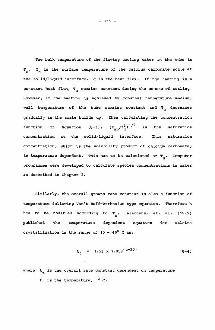
215
The bulk temperature of the flowing cooling water in the tube is
T0. is the surface temperature of the calcium carbonate scale at
the solid/liquid interface, q is the heat flux. If the heating is a
constant heat flux, Tg remains constant during the course of scaling.
However, if the heating is achieved by constant temperature medium,
wall temperature of the tube remains constant and Tg decreases
gradually as the scale builds up. When calculating the concentration2 1/2function of Equation (8-3), (K^/f^) .is the saturation
concentration at the solid/liquid interface. This saturation
concentration, which is the solubility product of calcium carbonate,
is temperature dependent. This has to be calculated at Tg. Computer
programmes were developed to calculate species concentrations in water
as described in Chapter 3.
Similarly, the overall growth rate constant is also a function of
temperature following Van't Hoff-Arrhenius type equation. Therefore k
has to be modified according to T^. Wiechers, et. al. (1*975)
published the temperature dependent equation for calcite
crystallization in the range of 10 - 40° C as:
kfc = 1.53 x 1.053(t_20) (8-4)
where k is the overall rate constant dependent on temperature
t is the temperature, ° C.

216
Therefore the first approximation of k modified by scale surface
temperature can be calculated according to Equation (8-4). From
Equation (8-4), koc = 1.98, therefore the corrected Zo
1.53 x 1.053 (t-20)1.98 x k (8-5)
If the scale adheres strongly onto the tube wall, the removal term in
general fouling equation such as Equation (6-3) can be ignored.
Therefore, the scaling rate of heat exchanger is:
kfdX___f _ dW 1 1de de * f(s) * Pf (8-6)
_ dW 1 J_ J_de de * f(S) * pf ’ kf (8-7)
where = fouling resistance, --- —---
e = time, s3= scale density, g/m
•9
k^ = thermal conductivity of scale, W/°C
8.3 SOME INVESTIGATIONS ON CALCIUM CARBONATE SCALING REPORTED IN THE
LITERATURE
8.3.1 Morse and Knudsen (1977)
Morse and Knudsen conducted scaling studies on a portable fouling
unit developed by HTRI (Coates et. al., 1980). The first section
consisted of an annular duct with a 1.91 cm I.D. outer glass and a
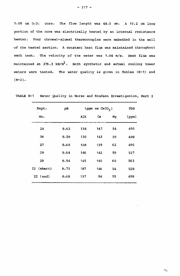
217
1.08 cm O.D. core. The flow length was 44.5 cm. A 10.2 cm long
portion of the core was electrically heated by an internal resistance
heater. Four chromel-alumel thermocouples were embedded in the wall
of the heated section. A constant heat flux was maintained throughout
each test. The velocity of the water was 1.04 m/s. Heat flux was
maintained at 276.3 kW/m . Both synthetic and actual cooling tower
waters were tested. The water quality is given in Tables (8-1) and
(8-2).
TABLE 8-1 Water Quality in Morse and Knudsen Investigation, Part I
Expt.
No.
pH (ppm
Aik
as CaC03
Ca
)
Mg
TDS
(ppm)
24 8.62 134 147 54 495
26 8.58 130 143 59 498
27 8.60 128 139 62 49028 8.64 146 142 59 527
29 8.54 145 140 64 563
22 (start) 8.73 187 146 54 52822 (end) 8.68 137 94 55 498
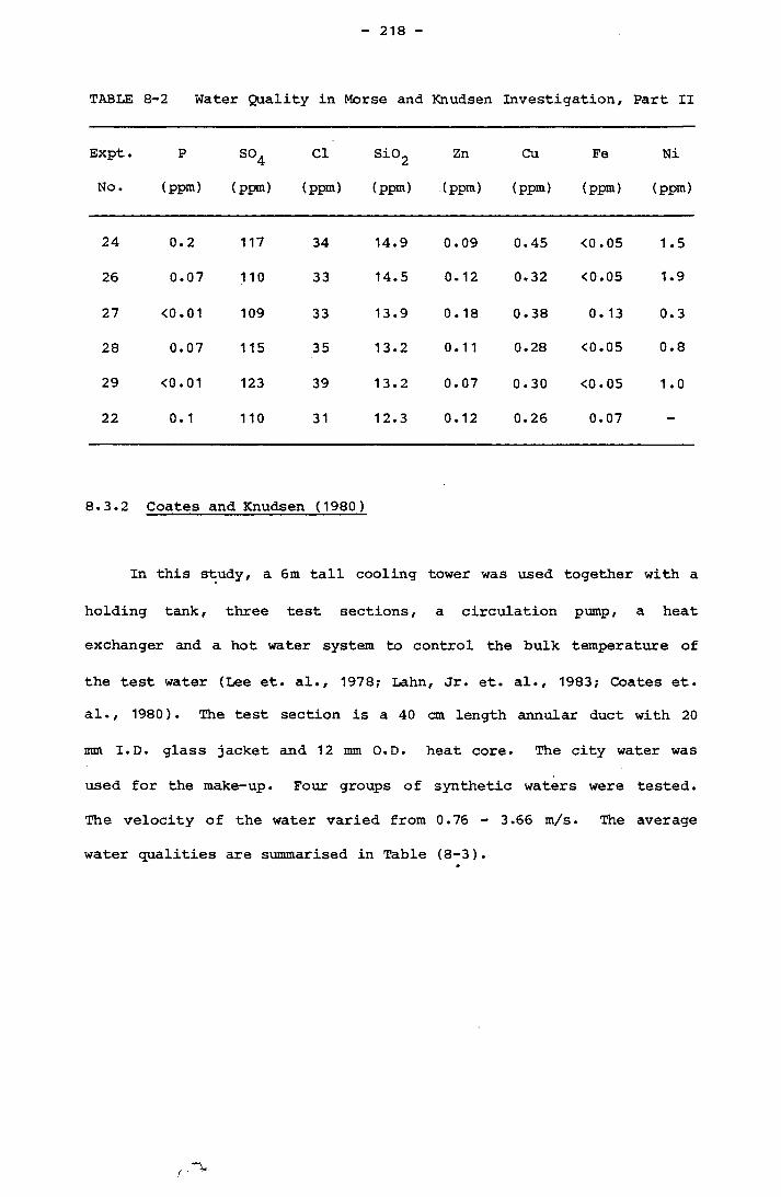
218
TABLE 8-2 Water Quality in Morse and Knudsen Investigation, Part II
Expt.
No.
P
(ppm)
SO,4(ppm)
Cl
(ppm)
Si02
(ppm)
Zn
(ppm)
Cu
(ppm)
Fe
(ppm)
Ni
(ppm)
24 0.2 117 34 14.9 0.09 0.45 <0.05 1.5
26 0.07 110 33 14.5 0.12 0.32 <0.05 1.9
27 <0.01 109 33 13.9 0.18 0.38 0. 13 0.3
28 0.07 115 35 13.2 0.11 0.28 <0.05 0.8
29 <0.01 123 39 13.2 0.07 0.30 <0.05 1.0
22 0. 1 110 31 12.3 0.12 0.26 0.07 -
8.3.2 Coates and Knudsen (1980)
In this study, a 6m tall cooling tower was used together with a
holding tank, three test sections, a circulation pump, a heat
exchanger and a hot water system to control the bulk temperature of
the test water (Lee et. al., 1978; Lahn, Jr. et. al., 1983; Coates et. al., 1980). The test section is a 40 cm length annular duct with 20
mm I.D. glass jacket and 12 mm O.D. heat core. The city water was
used for the make-up. Four groups of synthetic waters were tested.
The velocity of the water varied from 0.76 - 3.66 m/s. The average
water qualities are summarised in Table (8-3).
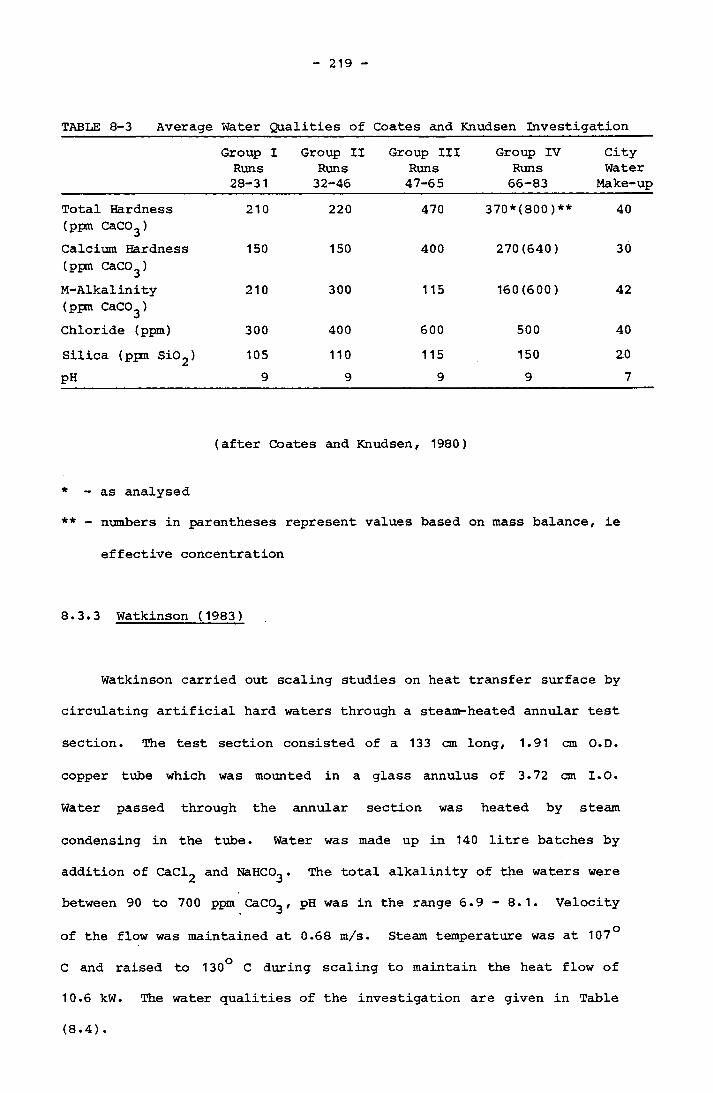
219
TABLE 8-3 Average Water Qualities of Coates and Knudsen InvestigationGroup I Runs28-31
Group II Runs32-46
Group III Runs 47-65
Group IV Runs66-83
CityWater
Make-upTotal Hardness 210 220 470 370*(800)** 40(ppm CaCC>3)Calcium Hardness 150 150 400 270(640) 30(ppm CaCO^)M-Alkalinity 210 300 115 160(600) 42(ppm CaCO^)Chloride (ppm) 300 400 600 500 40Silica (ppm SiC>2) 105 110 115 150 20pH 9 9 9 9 7
(after Coates and Knudsen, 1980)
* - as analysed** - numbers in parentheses represent values based on mass balance, ie
effective concentration
8.3.3 Watkinson (1983 )
Watkinson carried out scaling studies on heat transfer surface by
circulating artificial hard waters through a steam-heated annular test
section. The test section consisted of a 133 cm long, 1.91 cm O.D.
copper tube which was mounted in a glass annulus of 3.72 cm I.O.
Water passed through the annular section was heated by steam
condensing in the tube. Water was made up in 140 litre batches by
addition of CaCl2 and NaHC03. The total alkalinity of the waters were
between 90 to 700 ppm CaCO^, pH was in the range 6.9 - 8.1. Velocity
of the flow was maintained at 0.68 m/s. Steam temperature was at 107°
C and raised to 130° C during scaling to maintain the heat flow of
10.6 kW. The water qualities of the investigation are given in Table
(8.4).
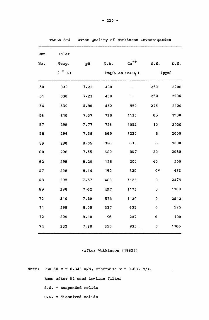
220
TABLE 8-4 Water Quality of Watkinson Investigation
Run
No.
Inlet
Temp.
( ° K)
pH T. A.
(mg/L as
Ca2 +
> CaCC>3 )
S.S. D.S.
(ppm)
50 330 7.22 400 - 250 2200
51 330 7.23 430 - 250 2200
54 330 6.80 450 950 275 2100
56 310 7.57 720 1130 85 1900
57 298 7.77 726 1055 10 2000
58 298 7.38 66 0 1230 8 2000
59 298 8.05 386 6 10 6 100060 298 7.55 680 86 7 20 2050
62 298 8.20 128 200 40 500
67 298 8. 14 192 320 0* 483
68 298 7.57 483 1123 0 2475
69 298 7.62 497 1175 0 1700
70 310 7.80 578 1130 0 261271 298 8.05 337 635 0 575
72 298 8. 10 96 207 0 100
74 332 7.30 350 835 0 1766
(after Watkinson (1983) )
: Run 60 v = 0. 343 m/s, otherwise v = 0.686 m/s.
Runs after 62 used in- line filter
S.S. = suspended solids
D.S. = dissolved solids
221
T . = 379° K at time zerosteam* not detected
8.4 COMPARISON OF CALCULATED AND EXPERIMENTALLY MEASURED SCALING RATE
The Lake Liddell water investigation (chapter 7) together with
the investigation reported in the literature (Section 8.3) provide
some data for calculating the rate of increase in fouling resistance
due to scaling. Data are selected from nearly pure CaC03 scaling
where no asymptotic fouling resistances are recorded. The overall
growth rate model mentioned in Section (8.2) is used for the
calculation. This is to compare the measured rates with the predicted
rates calculated by Hasson's ionic diffusion model. The results are
given in Table (8-5). Figures (8-2) and (8-3) plot the measured and
predicted scaling rate calculated by overall growth rate model and
Hasson's ionic diffusion model respectively.
From Figures (8-2) and (8-3), overall growth rate model seems to
overestimate the scaling rate. In many instances, especially data
obtained from the experiments of Coates and Knudsen; and Watkinson
indicate an overestimation by as factor of 5 or more (see dotted
line). On the other hand, the ionic diffusion model of Hasson—6 2predicts the scaling rate fairly well below 4 x 10 m °C/KJ although
more than 50% of the predicted rates are less than the measured rates
(a factor of 2-6 as indicated by the dotted line).
The overall growth rate model has been employed using a value of
rate constant calculated from the batch precipitation experiment. The
rate constant calculated is based on total crystal surface area. For
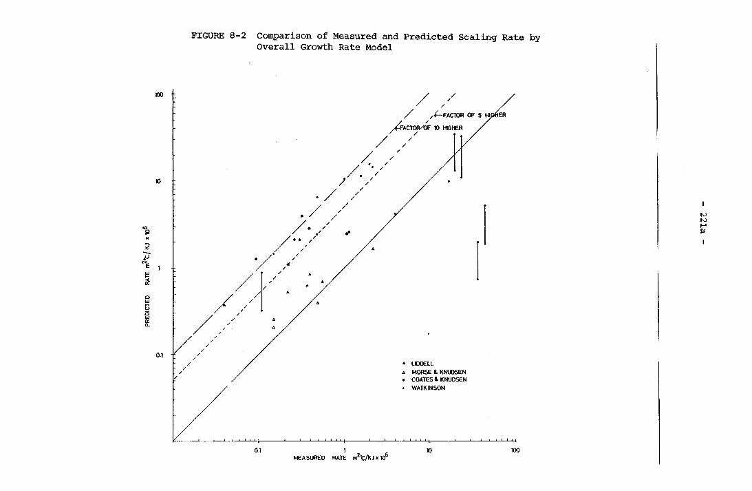
Overall Growth Rate Model221a
>1ja<D+jtoPStT>c■HrH(0oC/i73<U-PO•H73<DU04CNICOsgHPm
82
- -b\ P ~E
890L * CM /O
.jUJ 3iV
b O
BlO
IQB
ad
'KJx

Ionic Diffusion Model221b
(1)-Pftcr>C-HrHfUoC/3•73-PCOW•PPrUft EE gO >1 U Amioo9g0Hft
MEASURED RATE m2#c/KJ xlQ*
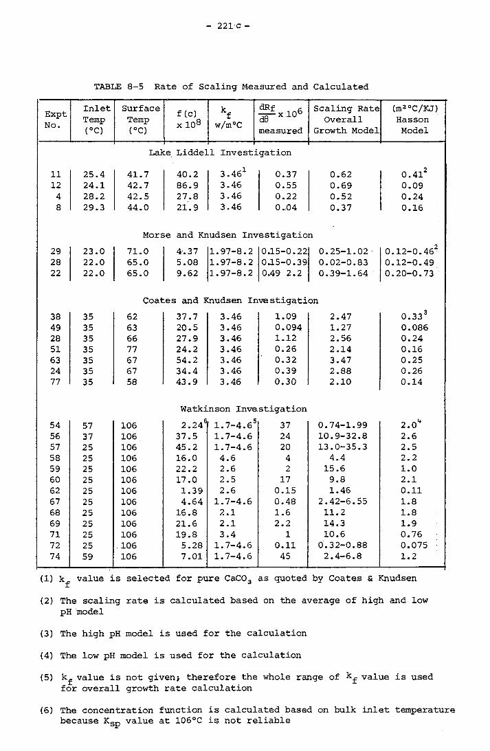
221 c -
TABLE 8-5 Rate of Scaling Measured and Calculated
ExptNo.
InletTemp(°C)
SurfaceTemp(°C)
f (c) x 108
kfw/m°C
dRf .^rxl°6measured
Scaling Rate Overall
Growth Model
(m2 °C/KJ) HassonModel
Lal<:e Liddej.1 Investigation
11 25.4 41.7 40.2 3.461 0.37 0.62 0.41212 24.1 42.7 86.9 3.46 0.55 0.69 0.094 28.2 42.5 27.8 3.46 0.22 0.52 0.248 29.3 44.0 21.9 3.46 0.04 0.37 0.16
Morse and Knudsen Investigation29 23.0 71.0 4.37 1.97-8.2 0.15-0.22 0.25-1.02 0.12-0.46228 22.0 65.0 5.08 1.97-8.2 0J.5-0.39 0.02-0.83 0.12-0.4922 22.0 65.0 9.62 1.97-8.2 0.49 2.2 0.39-1.64 0.20-0.73
Coates and Knudsen Investigation38 35 62 37.7 3.46 1.09 2.47 0.33349 35 63 20.5 3.46 0.094 1.27 0.08628 35 66 27.9 3.46 1.12 2.56 0.2451 35 77 24.2 3.46 0.26 2.14 0.1663 35 67 54.2 3.46 0.32 3.47 0.2524 35 67 34.4 3.46 0.39 2.88 0.2677 35 58 43.9 3.46 0.30 2.10 0.14
Watkinson Investigation54 57 106 2.246 1.7-4.6 5 37 0.74-1.99 2.0456 37 106 37.5 1.7-4.6 24 10.9-32.8 2.657 25 106 45.2 1.7-4.6 20 13.0-35.3 2.558 25 106 16.0 4.6 4 4.4 2.259 25 106 22.2 2.6 2 15.6 1.060 25 106 17.0 2.5 17 9.8 2.162 25 106 1.39 2.6 0.15 1.46 0.1167 25 106 4.64 1.7-4.6 0.48 2.42-6.55 1.868 25 106 16.8 2.1 1.6 11.2 1.869 25 106 21.6 2.1 2.2 14.3 1.971 25 106 19.8 3.4 1 10.6 0.7672 25 106 5.28 1.7-4.6 0.11 0.32-0.88 0.07574 59 106 7.01 1.7-4.6 45 2.4-6.8 1.2
(1) kf value is selected for pure CaC03 as quoted by Coates & Knudsen
(2) The scaling rate is calculated based on the average of high and low pH model
(3) The high pH model is used for the calculation
(4) The low pH model is used for the calculation
(5) kf value is not given; therefore the whole range of k^ value is used for overall growth rate calculation
(6) The concentration function is calculated based on bulk inlet temperature because KSp value at 106°C is not reliable

222
calculation of this scaling rate of the tube under fully turbulent flow conditions/ the tube surface area is used instead of the crystal surface area. It is evident that from the photomicrogram of the scale
taken by scanning electron microscopy/ scale is an aggregate of single calcium carbonate crystals (see Appendix E). Watkinson (1983)
reported that the deposits consist of crystals of 50-100 microns in size. The actual crystal surface areas of the crystals can be a
factor of 5 or more higher than the covered tube surface. The equation
dW 1 dQ * f(S) Kg f(C> (8-8)
is used to calculate the rate of calcium carbonate deposition. f(S) is a constant which is taken as the surface area of the tube. When crystals cover the tube surface, f(S) due to crystals are higher than f(S) of the tube and continue to increase with crystal growth and as new crystals are forming. As a result, ~ ^ ^ y is always higher
than the rate calculated if the actual crystal surface is known. This is considered to be the probable reason that the overall growth rate
model tends to overestimate the scaling rate as indicated in Figure (8-1 ) .
Another approach to calculate the scaling rate was proposed by
Hasson et al (1978). They considered mass transfer of ionic species in the fluid flowing through the pipe. Crystal growth can be
described by mass transfer of the ionic species in the supersaturated solution by Equation (6-62).
223
1 dWf(S) de “ Kd (cb ' ci) (6-62)
where K, is the mass transfer coefficient df(S) is the surface area
c, is the bulk concentration bc. is the interfacial concentrationi
Hasson determined the mass transfer coefficient for the ionic
species in the water flowing through the tube by applying the j-factor
analogy (see equation (6-67)). The unknown interfacial concentration
is avoided by combining the equation for a surface reaction (equation
(6-63)). The convective mass transfer coefficient of CaCO^ determined
is based on tube surface area. However, as the crystals deposit and
grow on the tube surface, the available mass transfer area increases.
As a result, more ions are able to be transferred onto a unit tube
surface area. Therefore the Hasson model is expected to underestimate
the actual scaling rate as indicated in Figure (8-3). This effect is
more apparent when the scaling rate is beyond 4 x 10 mz °C/KJ because of the significant build up of deposited crystals - hence a
significant increase in actual mass transfer surface. As a result,
the model predicted the scaling rate an order of magnitude lower than
the actual scaling rate indicated in Figure (8-3).
In comparing the overall growth rate model and Hasson's ionic
diffusion model, the main transfer coefficient obtained from the j-
factor analogy is based on well established physical data and
consequently more reliable. The equations used (Equations (6-69) and2-(6-71)) indicate that Kd and [CO3 ] are the two major terms that
determine the results, the reaction constant, Kr plays an

224
insignificant role in the equations. Therefore, the predicted scaling rate by Hasson's ionic diffusion model is less susceptible to the values of the reaction constant used as well as to the accuracy of the
chemical compositions of the water. On the other hand, the overall growth rate model uses kinetic values obtained from a different system, ie a batch reactor. The overall growth rate constant is also subject to uncertainty beyond 40° C. The predicted scaling rate is also strongly determined by the function of concentration, f(C)
(Equation (8-2)). The accuracy of the chemical composition of the water becomes critical for the scaling rate prediction by the overall growth rate model. In most cases, the pH values strongly influence
the final values of the concentration function calculated, this is particularly true for the data from the experiments of Coates and Knudsen and of Watkinson. The former reported approximate pH values for their experiments and the latter conducted the experiments on a
106° C heat transfer surface which requires a considerable extrapolation of the value of overall growth rate constant of calcite determined from the batch precipitation experiments. In view of all
these, until more reliable kinetic data is obtained for the flow- through-pipe system, Hasson's ionic diffusion model is considered to
be the more reliable.
Despite these difficulties associated with the use of the overall
growth rate model the basic concepts embodied in this approach are still valid for flow through pipe systems. The overall growth rate
model can still be used in parallel with the Hasson's diffusion model
to counter check the possible underestimation by Hasson's diffusionmodel.

8.5 EFFECT OF SURFACE TEMPERATURE AND VELOCITY
From the investigation of the scaling potential of Lake Liddell
water described in Chapter 7, heat transfer surface temperature is an
important factor in causing scaling in heat exchangers. The possible
threshold expressed as Larson and Buswell’s Langelier Index is 1.69
under test conditions. This number can be checked with data from
Morse and Knudsen as well as Coates and Knudsen Investigation (Table
8-6). In Morse and Knudsen investigation, Langelier Indexes
calculated at bulk inlet temperature indicate no scaling if compared
with 1.40 (Larson and Buswell's Langelier Index) and 1.25 (Ion Pair
consideration Langelier Index) determined from Chapter 7, but when
surface temperature is considered, the index number is 1.69. Runs 22,
28 and 29 precipitated calcium carbonate scale in the test secton,
whereas Runs 24, 26 and 27 did not scale. This tends to suggest 1.68
is a possible threshold of scaling under the test conditions.
Therefore, only calculating the Langelier Index of cooling water at
bulk inlet temperature can be deceptive in determining the water
scaling potential.
Langelier Indexes calculated from Coates and Knudsen data show
that water is highly supersaturated for bulk precpitation to take
place. However some of the runs actually did not scale at all.
Scaling in general is considered a combined result of bulk
precipitation in the system and wall crystallization on the heat
transfer surface. If wall crystallization which is the main mechanism
of adherent scale not prevailing, the precipitate due to bulk
precipitation may not be able to adhere onto the tube surface under
the effect of fluid shear stress. The Reynolds numbers and shear
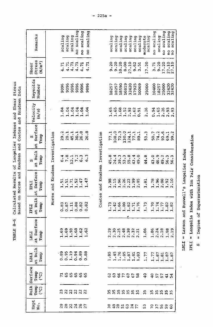
TAB
LE 8-6
Calcul
ated
Resu
lts of
Lang
elie
r Inde
xes an
d She
ar St
ress
B
ased
on M
orse
and Kn
udse
n and C
oate
s and K
nuds
en Da
ta225a
Rem
arks
scal
ing
scal
ing
scal
ing
no sca
ling
no sc
alin
g no
scal
ing
scal
ing
scal
ing
scal
ing
scal
ing
scal
ing
scal
ing
scal
ing
mod
erat
esc
alin
gno
scalin
g-
scal
ing
no sc
alin
g no
scal
ing
no sc
alin
g
Shea
rSt
ress
(N/m
2) rH H t—1 H i—I H OOOOOCNH O r-HOOOOcn cn in o h ^ i/i cm r^- cm cm h h
CT\<Xioaor-~<7im r- ro <Ti r- r-rH (M rH rH CM <M
Rey
nold
sN
umbe
r
9096
9096
9096
9096
9096
9096
1825
718
257
1859
016
819
3242
017
925
1006
925
000
1040
018
257
2500
032
420
3242
0
Vel
ocity
(m/s
) m in co <n n (M h in o o cooooooo lo cr> co <n cm <y> co cm cn cti
H rH H rH H H rHrHHHCMHO CM O H CM CM CM
Sat
Surf
ace
Tem
p
ciga
tion
29.2
29.1
45.1
30.1
26
.826
.8
:igat
ion
77.1
108.
072
.313
0.0
124.
177
.189
.153
.350
.774
.293
.669
.199
.2
Sat
Bulk
Te
mp
-M -Mw cn<u o> cf co h ni m co co ^ cn rn co ^ o oo o cm n mh vo i cm id mo ^ in ^ oi n m n in ^ m vo cn >x>
rH cm cn in in m1 ^ M* M1 m inc cCD CD
IPLI
at Su
rfac
e Te
mp
;e an
d Knu
ds
1.51
1.51
1.71
1.52
1.
471.
47
is and
Knud
s
1.98
2.15
1.96
2.26
2.22
1.99
2.05
1.81
1.78
1.96
2.08
1.92
2.10
IPLI
at Bu
lk
Tem
pI
Mor
s
0.83
0.87
1.11
0.88
0.82
0.82 C
oats
1.73
1.42
1.66
1.80
' 1.82 1.71
1.76
1.73
1.70
1.74
1.77
1.
821.
82
LBLI
at Su
rfac
e Te
mp
I
1.69
1.69
1.93
1.68
1.62
1.62
2.29
2.30
2.25
2.48
2.38
2.32
2.21
1.86
1.86
2.24
2.18
1.98
2.19
LBLI
at Bu
lk
Tem
p
0.89
0.95
1.19
0.94
0.89
0.88
1.85
1.45
1.76
1.85
1.87
1.81
1.83
1.77
1.77
1.87
1.81
1.87
1.87
Surf
ace
Tem
p(°
C)
71 65 65 65 65 65 62 63 66 77 67 67 58 40 40 57 57 41 54
Bul
kTe
mp
(°C
)
23 22 22 22 22 22 35 35 35 35 35 35 35 35 35 35 35 35 35
Expt
No. © co cm 'll! co f' oocTicOrHcn^r^ m o o o o
CM CM CM CM- CM CM O CM in CD CM in o in in CD
LBLI
= La
rson
and B
usw
ell's
Lang
elie
r Inde
x IP
LI =
Lang
elie
Index
with
Ion Pa
ir Con
side
ratio
n

226
stress are calcualated according to the fluid dynamics equations
developed for fully turbulent flow in the circular tube. The friction
factor calculated is increased by 8 percent in order to apply the
concentric annular ducts (Olson, 1973). The equations used are
presented as follows:
vDRe = — (8-9)v
where V is velocity, m/sD is tube diameter, in the case of concentric annular duct,
the hydraulic diameter, m2v is the kinematic viscosity of the water, m /s
0 .316' = Re1/4 (8-10)
where f is the friction factor
fpv28 (8-11)
2where t is shear stress, N/m3p is the water density, kg/m
The smallest shear stress encountered in Coates and Knudsen2 2investigation is 3.51 N/m of run 77 and 3.71 N/m of run 70.
According to Suitor et. al. (1977) who explained the anomaly regarding
asymptotic fouling corresponding to Reynolds numbers reported by
Hasson et. al. (1978) and Watkinson, et. al. (1975), the shear stress
is the most likely reason for asymptotic fouling. Suitor et. al.
227
(1977) reported the presence of threshold shear stress between 0.685 - 20.847 N/m below which no asymptotic fouling was observed. Therefore
it is possible that in run 7 0, precipitates due to bulk precipitation
were swept away by the high shear stress of the flow. On the other
hand, run 77 encountered wall crystallization of calcium carbonate on
the heat transfer surface and produced an adherent scale. This is
evident from the Langelier Index calculated at the surface
temperature. For run 77 the Langelier Index was 2.21 compared to 1.86
for run 70. However 1.86 is higher than the 1.69 or 1.68 in the case
of Morse and Knudsen's investigation. For Runs 56, 59 and 60, even
higher Langelier Indexes are tolerable without scaling. This might be
due to the very high shear stress of these runs which swept away even
the wall crystallization nuclei before they could grow into an
adherent scale. A bulk temperature of 35° C was used in Coates and
Knudsen investigation (Coates and Knudsen, 1980) compared to 22° C in
the Morse and Knudsen investigation (Morse and Knudsen, 1977). In the
batch precipitation of calcium carbonate experiments the crystals of
calcium carbonate produced at 35° consisted of at least 50% aragonite for solution supersaturation which is conducive to bulk precipitation.
Although the crystalline form was not investigation it is possible
that the scales formed in this investigation contain some aragonite
and subsequently are less adherent compared to calcite which was the
likely product of the Coates and Knudsen investigation. Therefore in
addition to the effects of water chemistry the combined effect of heat
transfer surface supersaturation and the fluid shear stress has to be
considered in order to assess the scaling potential of a particular
cooling water.

228
The surface nucleation on heat exchangers was studied by Chandler
(1964) using concurrent flow of warm saturated test solution and
cooling water. The test solution flowed through the annular section
of the heat exchanger over the cold tube surface. Supersaturation was
created on the tube surface and where a scale formed. Chandler showed
that the nucleus formation rate is a power function of surface
super saturation
K(8-12)f(Re) A°n (8-12)
where N°
0
K(8-12)
f (Re)
Ac
n
is the number of nuclei is the time
is a constant
is a function of Reynolds number
is the supersaturation of solution at the surface
defined by Chandler
is the empirical index for the solution studied.
Because the surface supersaturation was created by a temperature
gradient across the film, the heat transfer coefficient will increase
for an increase in Reynolds number. Chandler defined the critical
heat transfer rate (q ^ ) as the heat transfer rate able to produce 2100 nuclei/ft hr on the surface. The critical supersaturation is the
2supersaturation required to cause a nucleation rate at 100 nuclei/ft
hr. From the modified Dittus-Boelter equation, film heat transfer0.8coefficient is proportional to Re * . Chandler suggested that if
-__ „ ... ...... _J____________ = Re<0 • 8critical surface supersaturationthen there was the theoretical possibility that by increasing the
229
turbulence, the critical heat transfer rate that caused scaling could
be increased. From his experimental study Chandler presented the
following two empirical equations:
qcrit “ K(8-13)Re°'43 <8-13)
Critical supersaturation <x (8-14)
Therefore, the increase in the turbulence can increase the non-scaling
heat transfer capacity of the surface. However the effect is also
partly offset by a lowering of the critical supersaturation. This is
obviously not applicable to the constant heat flux test section
designed for the scaling studies. In those experiments the surface
temperature of the scale can be maintained (Fischer, et. al., 1975).
However, the actual heat exchanger used in industry relies on
temperature gradient as well as the effect of turbulence to achieve
heat transfer. Therefore there are advantages to increase the
velocity of the cooling water. Apart from the higher shear stress
introduced onto the tube surface to remove the scaling nuclei, in
general there is an increase in non-scaling heat transfer capacity on
the surface.
8.6 WALLERAWANG POWER STATION - ELECTRICITY COMMISSION OF NSW
The cooling towers are used in this power station to dissipate
the waste heat. By March 1983, Wallerawang No. 7 condensers
experienced back pressure and problems of higher temperatures
condensate. Inspection of the condensers revealed considerable
scaling (Little, 1984). Condenser tubes were cleared by specially
230
designed metal scrapers (pushed through by water pressure) and removed
700-800 g of scale and mud per tube. Analysis showed that this
material is approximately 70% calcium carbonate. A high manganese
content in the expelled scale/mud indicated the possible involvement
of chemical or biological manganese precipitation. The quality of the
cooling water between March 1982 and March 1983 are given in Table
(8-7). If a temperature of 43° C of the standard low pressure steam
is considered, the average condenser tubes wall temperature is
approximately 39° C. This is calculated as follows:
Inlet temperature = 25° C
Outlet temperature = 35° C
Saturated steam temperature = 43° C
Average temperature of the water = 30° C
The overall heat transfer coefficient based on outside diameter was
calculated by the Electricity Commission of NSW for 25.4 mm O.D. Al-
brass tubes for a water velocity of 1.28m/s at temperature of 21° C using the equation
U = C / (Velocity) (8-15)
where C = 2623.8 (Heat Exchanger Institute, 1978). The calculated UQ
is 2968.5 W/m2 °C.
For the inlet temperature of 25° C, Uq = 2968.5 x 1.03 = 3057.6
where 1.03 is the correction factor (Heat Exchanger Institute, 1978).
The physical properties of water at 30° are:

TABLE 8-7 Water Quality of Wallerawang Power Station No. 7 Cooling Tower
Date pH Cond.(ys/m)
M.O.Alkalinity (ppm CaCOa)
TotalHardness (ppm CaC03)
CaHardness (ppm CaC03)
soj-ppm
Clppm
Si02ppm
4.3.82 8.6 150,000 138 490 250 487 72.8 1310.3.82 9.0 115,000 142 400 210 622 66.8 10.516.3.82 8.9 180,000 153 600 280 784 104.7 156.5.82 7.85 28,000 - - 65 48 - -
14.5.82 8.4 85,000 158 470 220 500 12.5 21.818.5.82 8.3 72,000 118 460 120 260 14 _
26.5.82 8.55 110,000 164 372 180 297 57 222.6.82 8.3 110,000 116 365 215 363 58 19.69.6.82 8.3 110,000 104 480 280 487 54.6 10.618.6.82 8.4 55,000 96 220 130 118 30.3 6.824.6.82 8.7 110,000 122 370 190 490 55 11.630.6.82 8.5 110,000 116 400 190 433 67 21.57.7.82 8.2 170,000 138 640 300 487 72.8 11.715.7.82 8.3 240,000 - - 410 720 - -23.7.82 8.7 340,000 224 1210 510 1190 174.5 32.827.7.82 8.65 420,000 196 1160 450 1298 211 44.24.8.82 8.5 360,000 190 1180 400 1149 149 6011.8.82 8.55 320,000 195 1200 450 1203 143 5320.8.82 8.65 285,000 210 1030 525 1041 152 55.526.8.82 8.6 245,000 195 910 410 1028 128 48.52.9.82 8.6 180,000 190 630 275 622 102 30.5
10.9.82 8.55 190,000 240 540 250 580 103 2223.9.82 7.8 120,000 80 520 265 527 81 2227.9.82 8.1 170,000 112 600 300 580 129 6
29.10.82 8.15 68,000 108 224 122 135 39.5 6.44.11.82 7.7 110,000 115 330 150 284 90 14.59.11.82 8.55 163,000 195 630 240 514 41 17
10.11.82 8.55 310,000 240 1150 500 1136 17.1 36.525.11.82 8.6 290,000 235 950 430 919 148 222.12.82 8.4 260,000 250 890 420 811 181 23.58.12.82 8.45 340,000 125 830 380 865 155 6.017.12.82 8.3 340,000 305 1350 630 1380 196 3123.12.82 8.3 320,000 230 1160 540 1190 190 20.529.12.82 8.5 290,000 - 1100 440 1030 - -
9.2.83 8.2 115,000 110 370 180 365 65 33.516.2.83 8.45 135,000 160 470 260 581 80 30.524.2.83 8.4 175,000 145 540 270 554 80 31.52.3.83 8.65 200,000 220 685 380 744 106 469.3.83 8.5 230,000 260 840 470 840 156 50.5
17.3.83 8.5 220,000 180 810 415 879 115 39.525.3.83 7.0 180,000 30 690 340 906 111 25.130.3.83 8.0 180,000 45 670 390 745 118 42
231
Density = 99 5.6 5 kg/m3
Viscosity = 0.798 x 10³ kg/m s
Thermal conductivity = 0.6145 J/m s °C
Specific heat = 4.186 x 10³
„ , * DiVp 0.02286x1 .28x995.65Reynolds number Re = ---- = ----------------------^ 0.798x10"3
= 3.65 x 10⁴
o
Prandtl number Pr = 5+ = 4 ■ 186 x103x0 .798x10~3k 0.6145
= 5.436
Preliminary estimates of water film heat transfer coefficient can be
calculated by the empirical correlation:
ii M 2/3 fej 14 0.023V l kJ W (DG/^)0-2
Omitting the corrections for tube length and for viscosity ratio:
0.023x1.28x995.65x4.186x103 (3 .65x1 0*4 )° *2 x (5.436 )2/3
The overall temperature decrease = 43 - 30 = 13° C
The temperature decrease over the water resistance:
AT
Tw
0.02530x3057.7 0.02286x4854.9 X (43-30) 9.1°C
T + A Ti = 30+9.1 = 39.1°C
The viscosity of the water at T^ is then:
232
0.653 x 10 kg/m s
The viscosity-correction factor = 0.9723
The corrected coefficient = 4720.5 W/m2 ° C The temperature drop over the water resistance and the wall
temperature become
AT
Tw
0.02530 x 3057.6 0.02286 x 4720.5 X (43_30)
= T + AT. = 30 + 9.3 =l
= 9.3°C
39.3°C
This is so close to the wall temperature calculated previously that a
second approximation is unnecessary.
Some Langelier Indexes of the water calculated at bulk
temperature, as well as tube wall temperature, are given in Table (8-
8). Data show that there were prolonged periods of high
supersaturation of the cooling water with respect to calcium
carbonate. From 23/7/83 to 26/8/1982, the arithmetic mean of Larson
and Buswell's langelier Index calculated at bulk temperature is 1.68
and 1.76 at heat transfer surface. From 16/11/82 to 23/12/1982, it is
1.57 and 1.64 respectively. From 2/3/83 to 17/3/83, it is 1.65 and
1.72 respectively. The condenser cooling water was maintained at a
positive Langelier Index for the rest of the period to prevent
corrosion. It is very likely that scaling began in the period from
23/7/82 to 26/8/82 because the water had the potential of both bulk
precipitation and wall crystallization of calcium carbonate. In
practice the power station condenser is operating at the higher flow velocity compared to the test rig (1.5 to 2.0 m/s compared to 0.5 m/s
in the case of the Liddell power station study). Therefore there will

- 232a
TABLE 8-8 Langelier Indexes Calculated for the Wallerawang Power Station
DateLBLI*
at Bulk Temp
LBLIat Surface
Temp
IPLI** at Bulk Temp
IPLIat Surface
Temp
Sat Bulk Temp#
Sat Surface
Temp##23.7.82 1.81 1.85 1.60 1.66 36.5 41.227.7.82 1.73 1.92 1.54 1.72 31.4 47.84.4.82 1.48 1.56 1.30 1.37 18.8 22.011.8.82 1.59 1.66 1.40 1.47 23.6 27.620.8.82 1.80 1.88 1.62 1.69 38. 1 44.326.8.82 1.62 1.69 1.43 1.50 25.1 29.2
16.11.82 1.74 1.82 1.55 1.62 33.1 38.625.11.82 1.72 1.80 1.55 1.62 32.7 38.02. 12.82 1.55 1.62 1.39 1.46 23.3 27. 18.12.82 1.26 1.33 1.10 1.17 12.0 14.017.12.82 1.65 1.73 1.46 1.53 27.8 32.423.12.82 1.49 1.56 1.31 1.37 19.4 22.7
2.3.83 1.72 1.79 1.55 1.61 32.4 37.69.3.83 1.71 1.79 1.54 1.61 32.8 38. 117.3.83 1.51 1.58 1.34 1.40 20.4 23.8
* LB LI stands for Larson and Buswell's Langelier Index
** IPLI stands for Ion Pair Consideration Langelier Index
# Calculated at 35° C
## Calculated at 39° C
233
be a higher shear stress. However, the heat flux is of a similar
order, hence there is no additional tolerance due to increase in
Reynolds number (Section (8.5)). It is likely that the shear stress oof 4.66 N/m calculated at 1.5 m/s for a 18 gauge Alumimum Brass tube,
owhich is already 5 times higher than at 0.5 m/s (0.93 N/m ) is still
insufficient to remove the calcium carbonate scale. Further evidence
was observed from the calculation of the threshold Langelier Index on
data reported by Morse and Knudsen (1977) (Section (8.5)). The shear2stress calculated was 4.71 N/m . After the formation of the first
layer of calcium carbonate nuclei on the heat transfer surface, the
scale continued to grow into a thick and adherent scale under the
positive Langelier Index. The involvement of chemical or biofouling
by manganese or the presence of clays worsens the situation because
this also provides the sites for wall crystallization and may even reduce the threshold surface Langelier Index (supersaturation).
In view of all these factors, a cooling water therefore requires
constant monitoring of water chemistry to ensure that langelier Index
thresholds for both bulk precipitation and wall crystallization are
not exceeded, although the surface threshold is considered more
critical under designed heat flux and flow rate. The water,
especially when a cooling tower is used, requires appropriate control
on biofouling because of the nature of the cooling tower.
8.7 EFFECT OF MAGNESIUM
Watkinson (1983) had reported his findings on the effect of
magnesium on scaling. He studied the effect on magnesium on both
scaling rates where bulk precipiation is encouraged (at 57° C) and low
234
scaling rate (2 5° C) . A range of Mg^+/Ca^ + ratios between 0 and 1
were studied and a significant minimum scaling rate was observed for a
Mg/Ca ratio of 0.2 at 57° C bulk temperature, a weak minimum wasobserved at 25° C. It is evident that at 57° C the presence of
magnesium reduced the scaling rate, however this is not so apparent at
25° C. It is known that Magnesium can change the crystal habit of
calcium carbonate from calcite to aragonite (Moller and Rajagopalan,
1975; Reddy and Nancollas, 1976), however a ratio of Mg/Ca exceeding 4
was required to change calcite to aragonite at 25° C (Moller andRajagoplan, 1975). From the calcium carboante precipitation study
(Chapter 5), there was no reduction in the rate of precipitation of
calcium carbonate due to equal molar concentrations of magnesium
present in experiments run at 700 r.p.m. The crystal habit is calcite
and was similar to the crystals formed under non-stirring conditions.
Again from the Lake Liddell water investigation (Chapter 7), the scale
samples observed under scanning electron microscopy are very similar
to the crystal habit (polyhedral) observed from the precipitation
experiment. No magnesium was detected in the scale sample (see
Appendix E) . In the Lake Liddell study, bulk precipitation did take
place. However, it is similar to precipitation of non stirred samples
due to the 4.6 m above-ground pool used to achieve evaporative
cooling. The water temperature is approximately 25° C. Together with
the finding of Watkinson, it seems that the presence of magnesium has
an insignificant effect to calcium carbonate scaling at 25° C within
the range of 0 to 1 Mg/Ca ratio. However there is significant
reduction in the scaling rate at 57° C. This is probably due to the
already predominant aragonite form at higher temperatures further
suffers blockage of magnesium cation during the process of
crystallization to slow down the rate of formation. Tn addition, the

235
aragonite form is of low mechanical strength compared to calcite and
therefore is less tenancious. The nett result is a significant reduction of scaling as observed by Watkinson. The reason for the minimum observed is not clear, but probably reflects the incorporation of magnesium into the calcium based scale.
236
CHAPTER 9
CONCLUSIONS AND RECOMMENDATIONS
9.1 CONCLUSIONS
The following list briefly describes the general conclusions
drawn from the discussion of results given in Chapter 5, 7 and 8.
Calcium Carbonate Precipitation Studies
1. The interfacial energy of calcium carbonate (calcite predominat-2ing precipitate) is 101 mJ/m as determined by visual induction
2period data and 110 nvJ/m as determined by latent period data.The recent published data on the interfacial energy by Sohnel and
Mullin (1978) and Sohnel and Mullin (1982) is within the range 83 , 2- 120 nvJ /m .
2. The interfacial energy of calcium carbonate vaterite predominat
ing precipitate) is 118 nvJ/m2 as determined by visual induction2period data and 114 mJ/m as determined by the latent period.
3. It is possible to obtain a reasonably accurate estimate of inter
facial energy of calcium carbonate by bulk precipitation using
the latent period data obtained from pH measurement.
4. The order of nucleation was found to be equal to 8 by plotting
logarithm of induction period against logarithm of supersatura
tion defined as S-1. Mullin and Ang (1976) used the same
approach to calculate the order of nucleation of nickel ammonium

237
sulphate and obtained a value of 3.2
5. The metastable limit of calcium carbonate is at the degree of
supersaturation (S) equal to 10, below which nucleation does not occur.
6. At low initial degrees of supersaturation (S < 25 ) at 25°C, the
bulk crystallization experiments invariably produced calcite cry
stals irrespective of stirring speed. Calcite is thermodynami
cally most stable at 25°C and 1 atmoshpheric pressure.
7. At higher initial degrees of supersaturation (S > 25 ) at 25°C,
the final product invariably consists of more than one type of
calcium carbonate. Both aragonite and vaterite were observed.
The product was either the mixture of aragonite and calcite or vaterite and calcite. The calcite form was always present but in
scattered proportion for the power input per litre within the
range of 0.10 to 0.48 J /L s. The power input variation was
achieved by changing the speed of stirring of the 6 2.3 mm diame
ter 6 blade turbine impeller in a 5.1 litre of liquid (Geometry
B) . However, when the power input was beyond 0.48 J/L s, the precipitate was predominantly vaterite with some calcite. At the
moderate power input of 0.32 J/L s generated by the 93.5 mm diam
eter 6 blade turbine impeller stirring the 5.1 litre liquid at
220 r.p.m. (Geometry A), when the initial degree of supersatura
tion was 76.4 and beyond, only calcite crystals were formed. The
details of the reactor and impeller geometry were defined in Chapter 4. Both the degree of stirring and the initial degree of
supersaturation affect the crystal product, however, the degree
of stirring as well as the pattern of stirring generated by dif
ferent impeller and reactor geometry seems to exert a greater
influence. The aragonite found in these batch experiments at

238
25°C appeared as aggregate of crystals in unique shape as the result of continuing outward growth of a bundle of aragonite cry
stals into the calcium carbonate rich environment.
8. The kinetics of bulk crystallization of calcium carbonate can be described by the Davies and Jones equation. The overall growth
rate constants are independent of the initial degree of supersa
turation and stirring speed (under fully suspended conditions).
Therefore the crystallization of calcium carbonate is confirmed
to be surface-reaction controlled.
9. The overall growth rates of calcium carbonate precipitation can
be determined by the spontaneous precipitation method with
results comparable with the values obtained from the seeded cry
stal growth method published in the literature (Reddy and Nancol- las, 1971; Nancollas and Reddy, 1971). The overall growth rate
of the vaterite predominating precipitate was found to be faster
than calcite/aragonite precipitate as well as the pure calcite
precipitate.
10. The overall growth rate constants calculated by simplified
overall growth rate method (Section (4.3.4)) were found to be3 2 2 3 2 211.5± 1.0x10 L /mole min m and 20.5±2.3X10 L /mole min m for
calcite and vaterite respectively.
11 . The overall growth rate constants calculated by overall growth
rate with the size consideration method (Section (4.3.5)) using
Microvideomat 2 image analyzer to measure the size distribution
of the final precipitate were found to be less reproducible. The
rate constants of calcite were found to be in the range 17.2 - 3 2 225.2x10 L /mole min m . The rate constants of vaterite were
3 2 2found to be in the range 28.3 - 40.2x10 L /mole min m .12. Kazmlierczak et. al. (1982) using a seeded precipitation
239
technique and reported the rate constant of calcite to be 3 2 217.811.2x10 L /mole min m . They also recalculated Nancollas
and Reddy (1971) results and reported the value of 3 2 215x10 L /mole min m . Comparing the results obtained from this
3 2 2research, the value 15x10 L /mole min m can be considered as the typical value of the calcite crystallization rate constant.
There is no value published on vaterite crystallization hence
comparison is not possible. However, using the values of calcite as the general guideline, the most probable value of vaterite
crystallization rate constants lie within the range 203 2 230x10 L /mole min m .
13. The simplified overall growth rate method for interpreting the
kinetic data generated by spontaneous precipitation experiments
can be recommended for general crystallization studies for its
reproducibility and simplicity. The accuracy can be improved if
the sampling of crystal suspension can avoid the effect of suc
tion and hence give rise a more representative sample.14. The reproducibility of the overall growth rate method with size
consideration may be improved if the final crystal suspension can
be sized and counted for a large quantity by using an instrument
such as Coulter counter to get a more representative crystal sur
face area.
15. At 220 r.p.m. using Geometry A, aragonite gradually became predominant, in the form of long needle-like aragonite aggregates
of irregular pattern as temperature increased from 36°C to
55.8°C. At 55.8°C, crystal products were 100% aragonite aggregates. These aragonite aggregates were different from the one
produced from 25°C experiments. They broke up easily into
discrete aragonite crystals indicating the formation of

240
aggregates was due to agglomeration rather then the continuing
growth of crystals as in the case of 25°C experiments.
16. The degree of mixing had an apparent effect on the number of nuclei generated. The number increased as stirring speed
increased from 300 to 700 r.p.m. in Geometry B stirred reactor.
However, very vigorous stirring had the opposite effect. At S =
25.6, 880 r.p.m. reduced the number of nuclei by an order of mag
nitude when compared to 500 r.p.m.
17. The stirrer-crystal collision was the major mechanism of secondary nucleation in the bulk precipitation. The empirical equa
tion describing the kinetics of secondary nucleation of calcium6 7 • 9carbonate was derived as J = 2.323x10 S where J is rate of
nucleation in number of nuclei per second, S is the degree of
super saturation, e is the power in J/L s and is the crystal
concentration in g/L. The correlation coefficient was 0.9713. This empirical equation is applicable for the range of power
input per unit volume of 0.10 to 1.31 J/L s and very low crystal
concentrations (<0.0021 g/L). The exponent of the degree of
supersaturation p=7.9 is in agreement with the order of homogene
ous nucleation expressed as the exponent of supersaturation (S-1)
determined by induction period measurement. The order of nuclea
tion determined is equal to 8.
18. The presence of magnesium in the molar concentration equal to
calcium was found to prolong the induction period. However, the increase in stirring speed minimized such effects. The induction
period was reduced sharply when the stirring speed was increased
from 400 r.p.m. to 500 r.p.m.19. There was a range of degrees of mixing represented by 400 to 500
r.p.m. using Geometry B of 1:1 Mg/Ca system in which aragonite

241
aggregates were the predominating crystallographic form at 25°C
and S=24. However, both the extremes of zero and vigorous stir
ring (700 r.p.m.) produced polyhedral calcite (combination of
prism with rhombodedron) which was the result of the survival of fast growing crystal faces which otherwise disappeared in pure
calcium carbonate system.
20. In a 1:1 Mg/Ca system, the kinetics of secondary nucleation
appeared to be different from pure calcium carbonate system.
21. In 1:1 Mg/Ca system at 25°C, there seemed to be no retardation of
calcite due to magnesium.
Investigation of Scaling Potential of Lake Liddell Water to Power
Station Condenser Tubes
322. A test rig consisted of a 3.55 m heating section and a 4.5 m
above ground pool water reservoir was used to simulate the Lid
dell power station cooling water system. The water from Lake
Liddell was tested for its scale forming potential over a broad
range of total alkalinity and total calcium content. The possible threshold level of scaling expressed as Langelier Index at
bulk inlet temperature was found to be 1.40 calculated by Larson
and Buswell empirical temperature and ionic strength correction
and 1.25 calculated with ion pair consideration.
23. The heat transfer surface temperature was found to be a critical
factor. Therefore threshold Langelier Index at heat transfer
surface was calculated. The threshold Langelier Index at heat
242
transfer surface was 1.69 by Larson and Buswell and 1.52 by ion
pair consideration.24. The cooling water of Lake Liddell power station cooling system
must not be operated at or beyond the experimental threshold
Langelier Index for the bulk of water.25. There was a critical degree of super saturation for the bulk of
water as well as heat transfer surface. The former was estimated
as 17.0 and the latter as 31.6
26. The scaling of calcium carbonate in the condenser tubes was the result of bulk precipitation as well as wall crystallization
under testing conditions. However, wall crystallization can be
solely responsible for scaling when the effect of heat transfer
surface temperature is apparent.
27. The profile of calcium carbonate scale thickness in the tube
increased along the tube from the inlet to the outlet of the
tube. This was in accordance with the bulk temperature profile
on the cooling water along the tube.28. The crystal habit of the scale observed by scanning electron
microscopy was found to be identical with the crystal habit of
the precipitate formed in the 1: 1 Mg/Ca batch precipitation
experiment at 700 r.p.m. at 25°C (Section (5.2.3)). The
polyhedral calcite was the combination of prism with rhombohedon
forms.
Prediction of Calcium Carbonate Scaling in the Heat Exchanger of a Cooling Water System

243
29. The overall growth rate model based on the growth rate calcium
carbonate described by surface reaction controlled mechanism was
developed for scaling rate prediction in the heat exchanger. The
growth rate constant of calcium carbonate was obtained from batch
precipitation kinetic study of calcium carbonate and modified by
the Van't Hoff-Arrhenius equation for the heat transfer surface temperature. This model was tested on the scaling rate data
obtained from Lake Liddel water investigation (Chapter 7) and
published data from the literature. Data were selected from cal
cium carbonate predominant scale to avoid the complication of the
removal of scale due to high fluid shear and less tenacious
scale. The model predicted well on some data but showed consistent overestimation of scaling rate when significant
discrepancy was evident. This was due to the underestimation of
the actual reaction surface area, which was the crystal surface
area deposited on the heat transfer surface compared to only the
heat transfer surface area.
30. The Hasson's diffusion model was also tested in parallel with theoverall growth rate model. The model predicted fairly well below
-6 24x10 m °C/KJ. However more than 50% of the data were less
than the actual scaling rate by a factor of 2 - 6. Beyond-6 24x10 m °C/KJ, the predicted values were an order of magnitude
less than the actual scaling rate. The discrepency is believed
to be again due to the failure to incorporate the actual depo
sited crystal surface area which is the actual mass transfer sur
face area instead of the surface of the tube. Nevertheless,
because of the more reliable mass transfer coefficient valueobtained from the j-factor analogy, this model is considered more
■"6 2reliable for moderate scaling rate (dR^/d0 < 4x10 m °C/KJ).
244
31. Before the actual reaction or mass transfer surface area built up
by the deposited crystal can be incorporated into either model,
the overall growth rate model can be used in parallel with the
Hasson's diffusion model to safeguard the possible underestimation due to Hasson's diffusion model.
32. The threshold Larson and Buswell Langelier Index based on heat
transfer surface temperature determined from Lake Liddell water investigation as 1.69 was checked against published data from the
literature. It seems that this number is valid (1.68-1.69) as
the threshold Langelier Index calculated according to the surface
temperature for other cooling water systems for the inlet water
at 30°C or less. When the shear stress on the surface due to the2velocity of the cooling water is higher than 4.71 N/m , it is
possible that the effect of shear stress that sweeps away the
deposited crystals and nuclei can increase the threshold
Langelier Index. The effect will be more evident if the bulkinlet temperature is at 35°C or more which normally causes the
formation of discrete aragonite crystals in the midst of calcite.
The resulting scale will be less tenacious and easily swept away
by the velocity shear stress. The threshold Langelier Index
under this condition (the data reported by Coates and Knudsen,
1980) was found to be 1.86 or more.
33. The threshold Larson and Buswell Langelier Index was also checked
against the actual operating data of the Wallerawang power sta
tion of Electricity Commission of New South Wales which experi
enced condenser tubes scaling. The shear stress calculated was24.66 N/m . The operating data showed substantial periods of time
when both Langelier Indexes based on bulk inlet and heat transfer
surface temperatures were above the threshold calculated from
245
Lake Liddell water investigation (1.68 and 1.76 respectively).
Therefore the threshold Langelier Index based on heat transfer
surface temperature (1.69) successfully explains and predicts the
scaling encountered.
34. In general, the constant heating medium heat exchangers will be
less susceptible to scaling if operating under high cooling water
velocity because of higher shear stress to remove the scale from
the surface as well as an increase in non-scaling heat transfer capacity on the surface.
35. The presence of magnesium has an insignificant effect to calcium
carbonate scaling at 25°C within the range of 0 to 1 Mg/Ca ratio.
9.2 RECOMMENDATIONS
The following are recommendations for further research into this
topic:
1. The growth rate constants of calcite determined by batch precipi
tation experiments are only available for the temperature range
from 10 - 40°C. At most heat transfer surfaces the temperatures
are greater than 40°C. Such information can be conveniently
obtained by seeded crystallization experiments at controlled
solution temperatures greater than 40°C.
2. A study of the kinetics of calcium carbonate crystallization is
needed to investigate the effects of impurities commonly encoun
tered in the surface waters. This will facilitate a more accu
rate assessment to the scaling potential when waters are used as
cooling water. The effect of temperature and power input also
requires further study.

246
3. The mechanism of calcium carbonate crystallization has been gen
eralized as surface-reaction controlled. The surfaces of the
crystals produced from relatively low degrees of supersaturation
show layering which indicates surface layer growth. However, it
is not clear as to what type of surface reaction is the rate
determining mechanism. Experiments can be designed to investigate
the crystal product at different degrees of supersaturation by
using scanning electron microscopy to observe the formation of
the cyrstal surfaces. This is able to serve as the starting point to identify whether the surface reaction is nucleation con
trolled or screw dislocation.
4. The accuracy of the spontaneous precipitation method for general
crystallization studies can be further improved by modification
of the sampling method and also the crystals sizing methods.
Further investigation is required to check the superiority for
particle sizing of using fast scanning Coulter counter directly
onto the final crystal suspensions as compared to the Microvi
deomat 2 image analyzer.
5. The spontaneous precipitation experiment at 25°C has special sig
nificance to power station cooling water systems. In power sta
tion cooling water systems when cooling towers are used as the
cooling device, the cooling water is recirculated in a closed-
loop pattern. The result of recirculation by pumps implies a
constant increase of calcium carbonate nuclei in the system similar to secondary nucleation in relation to the power input stu
died by the batch spontaneous precipitation experiments. Because
of the coexistence of bulk precipitation and wall crystallization
in many calcium carbonate scaling situations, the role of bulk
precipitation has to be described by secondary nucleation in the
247
cooling water system. Further study is required to relate the
secondary nucleation of calcium carbonate to the cooling water
systems. Such studies can be carried out on a test rig similar
to the test rig described in Chapter 7 using various pumping
speeds (r.p.m.) for a specified cooling water composition. The
number of nuclei in the flow can be counted with respect to time
to observe the transient increase/decrease of nuclei due to the
power input. Two experiments can be carried out in parallel for
each pumping speed, with heating and without heating, to deter
mine the contribution of scaling due to bulk precipitation under similar test conditions.
6« The water chemical compostions calculated based on thermodynamic
equilibria of the salts present can be improved by incorporating additional species such as silicate. The effect of magnesium on
calcium carbonate precipitation has been investigated and
reported (Moller and Rajagopalan, 1975; Reddy and Nancollas,
1976; Reddy and Wang, 1980; Watkinson, 1983). However, more work
is still required to relate the effect of magnesium on calcium
carbonate precipitation to calcium carbonate scaling in the heat exchangers. The effect of silicate can be significant, yet such
information is very scarce. The presence of such foreign com
pounds will alter the rate of crystal growth as well as the tena
city of the scale.
7. The effect of heat transfer surface temperature on the formation
of different crystallographic calcium carbonate crystals requires
further investigation. This project has already indicated the
significance of heat transfer surface temperature in predicting
the scaling potential. Therefore, more information in this area will enable accurate predictions to be made.
248
8. The velocity shear stress of the cooling water plays a signifi
cant role in preventing or reducing the growth of calcium carbonate scale on the heat transfer surfaces. The precipitation
experiments in Chapter 4 indicates that the formation of crystal
habits are closely affected by the degree of mixing and tempera
ture. Experiments PE18 and PE19 even suggested the possibility
to encourage the formation of discrete acicular aragonite in the
presence of magnesium by manipulating the degree of mixing. This
implies that the formation of scale for certain velocities will be weak and easily removed due to the presence of the loosely
formed aragonite. Further research is required to establish an
optimal velocity related to a range of calcium carbonate deposits
from pure calcium carbonate to mixtures of magnesium and calcium
carbonates and silicates. The degree of tenacity of scale related to crystal composition and forms as the result of velo
city (analogous to the degree of mixing in the stirred reactor
experiments) can subsequently provide a more realistic estimate
of the fouling factor due to calcium carbonate scaling for heat
exchanger design.
9. The actual reaction or mass transfer surface area represented by
the deposited crystal surface areas on the heat transfer surfaces
have to be incorporated into either the overall growth rate model
or the Hasson's diffusion model for accurate prediction of the
rate of scaling.
249
NOTATION
a
a
a
a
solsod
A
A'
CAlk]bb'
cco
c.1
cm
1
1
Exponent
Activity of the solution Activity of the solid
Mean distance of closest approach
Surface area
Cross sectional area of the flow stream
ConstantTotal alkalinity in equivalents per litreSlope of solubility curve
Cooling rateAdherence parameterConstantNucleation rateConcentration at any given time Incoming concentration Bulk concentrationInterfacial concentration; molar concentration of ionic spe cies with chargeConcentration greater than the saturated concentration but
below which nucleation does not occurConcentration of material which undergoes the reaction Surface concentration; saturated concentration
Initial concentrationEquilibrium concentration of surface adsorbed molecules at
the given temperatureConcentration of the liquid at temperature t^Hypothetical concentration of the liquid saturated with sea ling component at temperature t^

250
c+c
c'+c'
c+sc-sc
AcddmdodPDDe
Concentration of the bulk cationConcentration of the bulk anion
Total concentration of the adsorbed cation
Total concentration of the adsorbed anion
Equilibrium concentration of the cation
Equilibrium concentration of the anion
Impeller distance off vessel bottomConstants
Specific heatTotal carbon
Initial total carbonSupersaturation
Particle diameterMolecular diameterLattice parameterParticle sizeMolecular diffusivity; impeller diameter
Equivalent diameter of the annular flow passageHydraulic diameterInside diameter of the tubeOutside diameter of the tube
Surface diffusion coefficientLogarithmic mean diameter of the tubeDifference in lattice parameter between solid and nucleusActivation energy of the reaction
Impact energy
Blasius friction factorMonovalent activity coefficient
Divalent activity coefficient
251
f± Mean activity coefficient
f (C) Function of the precipitation solute concentration
f (S) Function of the available surface area during crystallization
G Linear growth rate
AG Free energy change*AG Critical free energy change
h Step height
h.1
Film coefficient of the inside tube
ho Film coefficient of the outside tube
ha.1
haO
Fouling factor of the inside tube
Fouling factor of the outside tube
Exponent
I Ionic strength
I.1 Chronomal of i order
J Number nucleation rate
J' Mass nucleation rate
JG Flux of solute on the surface of the crystal
JK Flux of solute away from the surface of the crystal
Jc-c Contact nucleation rate due to crystal-crystal collision
Jc-ms Contact nucleation rate due to collision of crystal-stirrer
collision
k Overall growth rate constant
k' Factor defined in Equation (4-112)
K" Gradient of overall growth rate equation with size considera
tion
kf Thermal conductivity of the deposit
km Thermal conductivity of the tube wall
kw Thermal conductivity of the water
kl - k3 First order rate constants in Equation (4-19)
252
k4
K
K(eq.
K
K
KK
K
d
GHn
KrKTKwKKK
1
2I
1
K
K4
5
l
1L
Rate constant in Equation (4-19)
Boltzman constant
nos.) ConstantWeight of the substance precipitated by cooling a unit volume
of saturated solution by 1°C
Mass transfer coefficient
Combined diffusion-reaction mass transfer coefficient
Henry's constantNucleation rate constantSurface reaction coefficient
Constant in Equation (4-116)Dissociation constant of water Dissociation constant of carbonic acid Dissociation constant of bicarbonateDissociation constant of carbonic acid corrected for activity coefficientDissociation constant of bicarbonate corrected for activity coefficient
oDissociation constant of CaCO^Rate constant of the formation of CaCO°/unit crystal surface
as defined in Equation (4-44)Constant of the Davies and Jones model
Solubility product of calcium carbonateSolubility product of calcium carbonate corrected for activity
coefficients
ExponentBlade length of the impeller Length; particle size
253
M
Mx
“tn0 n1
n*n
nm
n
N
NPPPPPP1d
Final crystal size
Initial crystal size Mean crystal sizeNormalized third moment of size distribution
Normalized third moment of size distribution of final size
Constant4th moment about zero of population distribution
Mass of crystal of size z which do not redissolve into solu
tionMolecular weightTotal crystal mass above size d^Solids concentrationExponent; particle populationNuclei population densityNumber of molecule in a nucleusNumber of molecule in a critical nucleusNumber of the monomerNumber of impeller blade for condition 1Number of impeller blade for condition 2Average population density in the size rangeImpeller speed; number of nuclei generated by one collision;
number of crystal per unit volumeNumber of crystal of L-HD
Power numberWetted perimeter; constant
Blade pitch of the impeller
Power input Metastable zone width
Probability factor
254
(Pr) f
Qqr*r
Ri
R
Rc
Re
(Re) f
s
S
S
SaSc
max
o
Prandtl number based on average film temperature
Volumetric flow rate
Heat flux
Radius of the nucleus
Radius of the critical nucleus
Standard gas constant
Dissolution rate
Crystal growth rate perpendicular to the surface
Thermal resistance due to the fouling deposit
Overall growth rate
Asymptotic fouling resistance
Reynolds number
Reynolds number based on average film temperature
Supersaturation defined in Equation (6-41)
Degree of supersaturation
Solute supersaturation in weight per unit volume
Degree of supersaturation based on activity
Schmidt number
Sherwood number
Temperature
Bulk temperature
Wall temperature
Inlet temperature
Maximum allowable undercooling
Absolute temperature; vessel diameter
Latency time
Surface temperature expressed in absolute temperature
Total molar calcium concentration
Overall heat transfer coefficient
Activation energy for the formation a kink
Overall heat transfer coefficient based on outside diameter
255
vvoo
VS
VVmVowwdP
zz
z12
Z
VelocityVelocity of a straight step of crystal growth
Fluid velocity averaged over the cross section of the pipe;
average speed of surface adsorbed
VolumeMolecular volumeInitial crystal growth velocity
Impeller blade width
Collision frequency of crystal with size d^
Mass of the crystal or scale deposit Dehydration energy of ions Dehydration energy of kinksWeight of total deposit (ionic diffusion and particulate)
Degree of precipitation Thickness of the depositMean diffusion distance on the surface in time 0 Thickness of the tube wall Step spacing ExponentValencies or charges of cation Valencies of charges of anion Liquid depth
Greek Symbol
a1
aa
a
N
t
a
Arbitrary constant characteristic of degree of precipitationwhen diffusion-controlled is valid
Gradient based on crystal numberGradient based on induction period
Particle volume shape factor
256
av3
V3
3r6
V6
e
e0
0
0
0
1
c
D
0
0
0
m
indlato
0PK
*<f>
<J>dr
P
P
PP
n
cf
w
ra
■a
T
0)
Particle surface shape factor Constant
Geometry shape factorRate of removal of molecules from molecular cluster
Length of diffusion path
DisregistryDissipated energy per unit mass/volume
Time
Time scaleTime constant characterizing the tenacity of deposit
Induction period of scaling in heat exchanger Retention time Induction period Latent periodCharacteristic time constant defined in Equation (6-78) Retention time of plug flow system
Contact angle FactorRate of depositionRate of removal of scale
DensityDensity of the crystal
Bulk density of deposit
Density of the fluid
Effective factor
Solid-liquid surface energyDegree of supersaturation defined as S - 1
Fluid wall shear stressApparent angular velocity of the spiral

257
\p Potential difference between crystal and the bulk solution
ip Function of the deposit structure
Y Kink retardation constantoy^ Chemical potential of the substance per molecule in the dis
solved state
y^ Chemical potential of the substance per molcule in the solid
state
y Normalized s moment about the meansDegree of supersaturation as defined in Equation (4-33)
Water characterization factor which is the function of Lan-
gelier Index
Z Strain between nucleus and solid particle
v Frequency of oscillations of the growth units in steps
A Amount of calcium carbonate remaining to be precipitated as
defined in Equation (4-16)
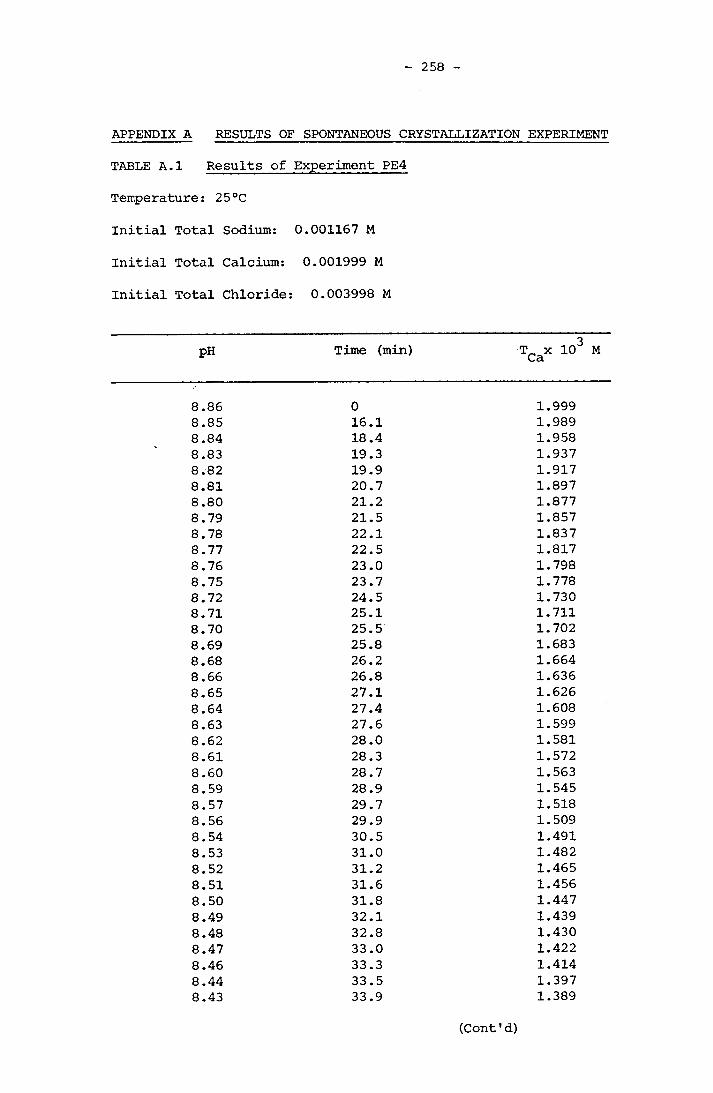
258
APPENDIX A RESULTS OF SPONTANEOUS CRYSTALLIZATION EXPERIMENT
TABLE A.1 Results of Experiment PE4
Temperature: 25°C
Initial Total Sodium: 0.001167 M
Initial Total Calcium: 0.001999 M
Initial Total Chloride: 0.003998 M
PH Time (min) T x 10' Ca
8.86 0 1.9998.85 16.1 1.9898.84 18.4 1.9588.83 19.3 1.9378.82 19.9 1.9178.81 20.7 1.8978.80 21.2 1.8778.79 21.5 1.8578.78 22.1 1.8378.77 22.5 1.8178.76 23.0 1.7988.75 23.7 1.7788.72 24.5 1.7308.71 25.1 1.7118.70 25.5 1.7028.69 25.8 1.6838.68 26.2 1.6648.66 26.8 1.6368.65 27.1 1.6268.64 27.4 1.6088.63 27.6 1.5998.62 28.0 1.5818.61 28.3 1.5728.60 28.7 1.5638.59 28.9 1.5458.57 29.7 1.5188.56 29.9 1.5098.54 30.5 1.4918.53 31.0 1.4828.52 31.2 1.4658.51 31.6 1.4568.50 31.8 1.4478.49 32.1 1.4398.48 32.8 1.4308.47 33.0 1.4228.46 33.3 1.4148.44 33.5 1.3978.43 33.9 1.389
(Cont' d)

TABLE A.1 (Cont'd)
8.42 348.41 358.40 358.38 368.37 368.36 368.34 378.33 388.32 388.30 398.29 408.28 408.27 418.26 418.25 428.24 438.23 438.21 458.20 458.19 468.18 478.17 488.16 498.15 508.14 518.13 528.12 548.11 548.10 588.09 598.08 618.07 648.067.95
66
1.3721.3641.3561.3401.3321.3241.3081.3001.2931.2851.2771.2591.2621.2551.2471.2401.2321.2251.2181.2101.2031.1961.1891.1831.1761.1691.1631.1561.1491.1371.1301.1241.117
,50427
,9826549494261771617170943649
equilibrated
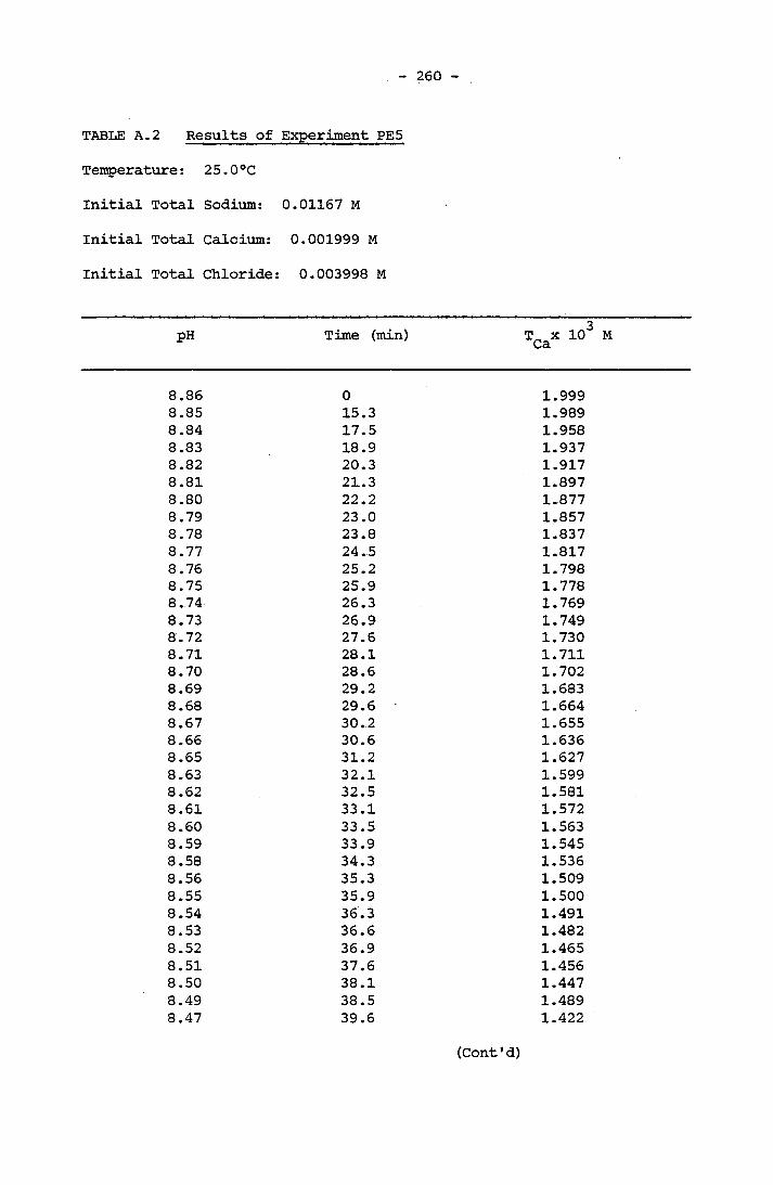
260
TABLE A.2 Results of Experiment PE5
Temperature: 25.0°C
Initial Total Sodium: 0.01167 M
Initial Total Calcium: 0.001999 M
Initial Total Chloride: 0.003998 M
pH Time (min) T x 10 Ca
8.86 0 1.9998.85 15.3 1.9898.84 17.5 1.9588.83 18.9 1.9378.82 20.3 1.9178.81 21.3 1.8978.80 22.2 1.8778.79 23.0 1.8578.78 23.8 1.8378.77 24.5 1.8178.76 25.2 1.7988.75 25.9 1.7788.74 26.3 1.7698.73 26.9 1.7498.72 27.6 1.7308.71 28.1 1.7118.70 28.6 1.7028.69 29.2 1.6838.68 29.6 1.6648.67 30.2 1.6558.66 30.6 1.6368.65 31.2 1.6278.63 32.1 1.5998.62 32.5 1.5818.61 33.1 1.5728.60 33.5 1.5638.59 33.9 1.5458.58 34.3 1.5368.56 35.3 1.5098.55 35.9 1.5008.54 36.3 1.4918.53 36.6 1.4828.52 36.9 1.4658.51 37.6 1.4568.50 38.1 1.4478.49 38.5 1.4898.47 39.6 1.422
(Cont'd)
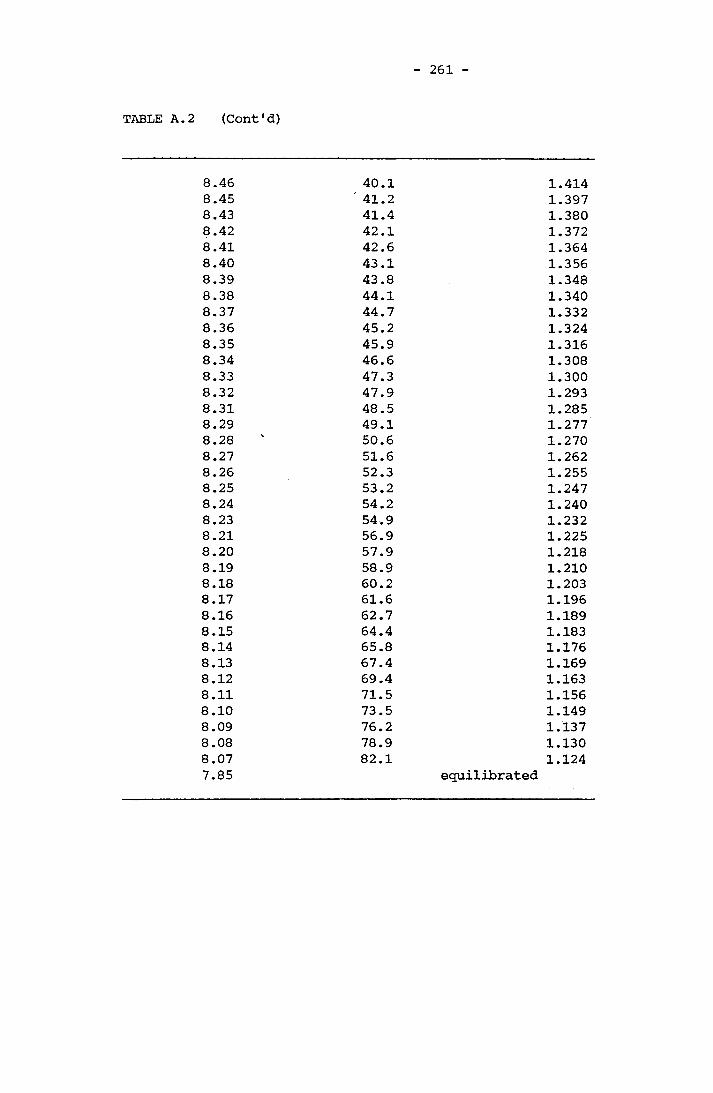
261
TABLE A.2 (Cont'd)
8.46 40.18.45 41.28.43 41.48.42 42.18.41 42.68.40 43.18.39 43.88.38 44.18.37 44.78.36 45.28.35 45.98.34 46.68.33 47.38.32 47.98.31 48.58.29 49.18.28 50.68.27 51.68.26 52.38.25 53.28.24 54.28.23 54.98.21 56.98.20 57.98.19 58.98.18 60.28.17 61.68.16 62.78.15 64.48.14 65.88.13 67.48.12 69.48.11 71.58.10 73.58.09 76.28.08 78.98.077.85
82.1
1.4141.3971.3801.3721.3641.3561.3481.3401.3321.3241.3161.3081.3001.2931.2851.2771.2701.2621.2551.2471.2401.2321.2251.2181.2101.2031.1961.1891.1831.1761.1691.1631.1561.1491.1371.1301.124
equilibrated
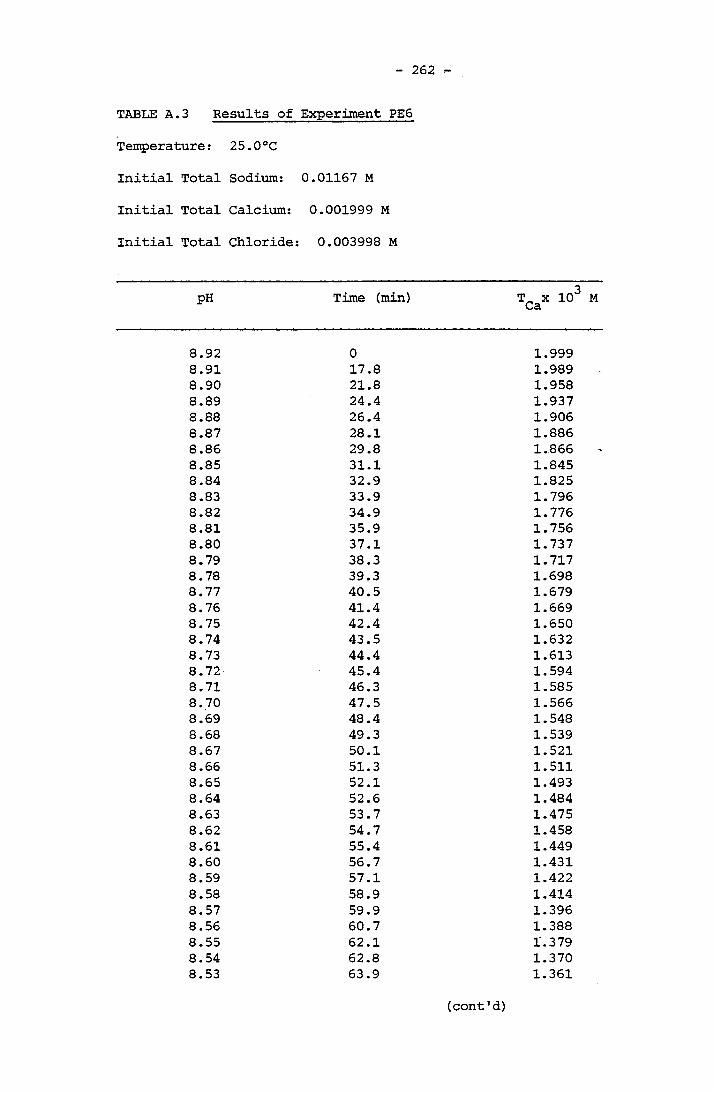
262
TABLE A.3 Results of Experiment PE6
Temperature: 25.0°C
Initial Total Sodium: 0.01167 M
Initial Total Calcium: 0.001999 M
Initial Total Chloride: 0.003998 M
PH Time (min) T_ x 10' Ca
8.92 0 1.9998.91 17.8 1.9898.90 21.8 1.9588.89 24.4 1.9378.88 26.4 1.9068.87 28.1 1.8868.86 29.8 1.8668.85 31.1 1.8458.84 32.9 1.8258.83 33.9 1.7968.82 34.9 1.7768.81 35.9 1.7568.80 37.1 1.7378.79 38.3 1.7178.78 39.3 1.6988.77 40.5 1.6798.76 41.4 1.6698.75 42.4 1.6508.74 43.5 1.6328.73 44.4 1.6138.72 45.4 1.5948.71 46.3 1.5858.70 47.5 1.5668.69 48.4 1.5488.68 49.3 1.5398.67 50.1 1.5218.66 51.3 1.5118.65 52.1 1.4938.64 52.6 1.4848.63 53.7 1.4758.62 54.7 1.4588.61 55.4 1.4498.60 56.7 1.4318.59 57.1 1.4228.58 58.9 1.4148.57 59.9 1.3968.56 60.7 1.3888.55 62.1 1.3798.54 62.8 1.3708.53 63.9 1.361
(cont'd)

TABLE A.3 (Cont'd)
8.52 648.51 658.50 668.49 678.48 698.47 708.46 718.45 728.44 738.43 748.42 758.41 768.40 778.39 798.38 808.37 828.36 838.35 848.34 858.33 878.32 898.31 898.30 918.29 938.28 948.26 988.25 1008.24 1028.23 1048.22 1078.207.85
111
1.3531.3361.3281.3191.3111.3031.2951.2861.2781.2701.2621.2541.2461.2381.2301.2231.2151.2071.1991.1921.1841.1771.1691.1621.1541.1491.1391.1321.1251.1171.110
8938231153498181267514126489624
equilibrated

264
TABLE A.4 Results of Experiment PE7
Temperature: 25.0°C
Initial Total Sodium: 0.01167 M
Initial Total Calcium: 0.001999 M
Initial Total Chloride: 0.003998 M
pH Time (min) T x 10 Ca
8.87 0 1.9998.86 12.5 1.9898.85 13.9 1.9688.84 15.1 1.9378.83 16.2 1.9178.82 17.1 1.8978.81 17.9 1.8778.80 18.6 1.8568.79 19.4 1.8368.78 19.9 1.8178.77 20.7 1.7978.76 21.4 1.7788.75 21.8 1.7588.74 22.5 1.7398.73 25.9 1.7298.72 23.5 1.7108.71 24.0 1.6918.70 24.4 1.6828.69 25.0 1.6638.67 26.0 1.6358.66 26.5 1.6168.65 27.2 1.6078.64 27.9 1.5898.62 28.6 1.5628.61 28.9 1.5528.60 29.4 1.5448.59 29.8 1.5268.58 30.4 1.5178.57 30.8 1.4998.56 31.4 1.4908.55 31.8 1.4818.54 32.4 1.4728.53 32.8 1.4638.52 33.5 1.4468.51 33.9 1.4378.50 34.4 1.4298.49 34.8 1.4208.48 35.3 1.4128.47 36.0 1.403
(Cont'd)

TABLE A.4 (Cont'd)
8.45 37.8.44 37.8.43 38.8.42 38.8.41 39.8.40 39.8.39 40.8.38 41.8.37 41.8.36 42.8.35 42.8.34 43.8.33 44.8.32 45.8.30 45.8.29 47.8.28 48.8.27 49.8.26 50.8.25 51.8.24 52.8.22 53.8.21 55.8.20 56.8.19 57.8.18 59.8.17 61.8.15 62.8.14 64.8.13 66.8.12 68.8.11 73.8.10 76.8.09 80.8.08 83.8.07 87.8.05 98.8.04 106.8.03 115.8.01 126.7.88
1.3871.3781.3621.3541.3451.3371.3291.3211.3131.3061.2981.2901.2821.2741.2671.2591.2521.2441.2371.2291.2211.2141.2071.1991.1921.1851.1781.1711.1651.1581.1511.1381.1321.1251.1191.1061.0991.0921.0861.079
2426284253993375320222588408666740999498
equilibrated
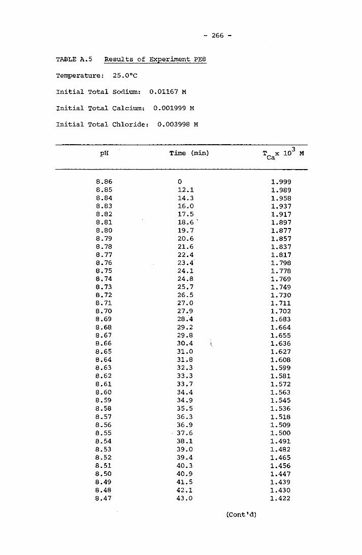
266
TABLE A.5 Results of Experiment PE8
Temperature: 25.0°C
Initial Total Sodium: 0.01167 M
Initial Total Calcium: 0.001999 M
Initial Total Chloride: 0.003998 M
PH Time (min) T x 10' Ca
8.86 0 1.9998.85 12.1 1.9898.84 14.3 1.9588.83 16.0 1.9378.82 17.5 1.9178.81 18.6 ' 1.8978.80 19.7 1.8778.79 20.6 1.8578.78 21.6 1.8378.77 22.4 1.8178.76 23.4 1.7988.75 24.1 1.7788.74 24.8 1.7698.73 25.7 1.7498.72 26.5 1.7308.71 27.0 1.7118.70 27.9 1.7028.69 28.4 1.6838.68 29.2 1.6648.67 29.8 1.6558.66 30.4 1.6368.65 31.0 1.6278.64 31.8 1.6088.63 32.3 1.5998.62 33.3 1.5818.61 33.7 1.5728.60 34.4 1.5638.59 34.9 1.5458.58 35.5 1.5368.57 36.3 1.5188.56 36.9 1.5098.55 37.6 1.5008.54 38.1 1.4918.53 39.0 1.4828.52 39.4 1.4658.51 40.3 1.4568.50 40.9 1.4478.49 41.5 1.4398.48 42.1 1.4308.47 43.0 1.422
(Cont'd)
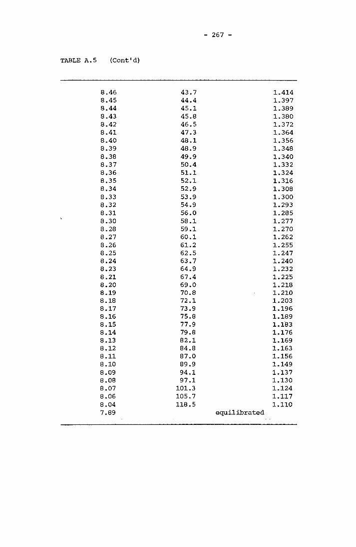
267
TABLE A.5 (Cont'd)
8.46 43.78.45 44.48.44 45.18.43 45.88.42 46.58.41 47.38.40 48.18.39 48.98.38 49.98.37 50.48.36 51.18.35 52.18.34 52.98.33 53.98.32 54.98.31 56.08.30 58.18.28 59.18.27 60.18.26 61.28.25 62.58.24 63.78.23 64.98.21 67.48.20 69.08.19 70.88.18 72.18.17 73.98.16 75.88.15 77.98.14 79.88.13 82.18.12 84.88.11 87.08.10 89.98.09 94.18.08 97.18.07 101.38.06 105.78.04 118.57.89
1.4141.3971.3891.3801.3721.3641.3561.3481.3401.3321.3241.3161.3081.3001.2931.2851.2771.2701.2621.2551.2471.2401.2321.2251.2181.2101.2031.1961.1891.1831.1761.1691.1631.1561.1491.1371.1301.1241.1171.110
equilibrated
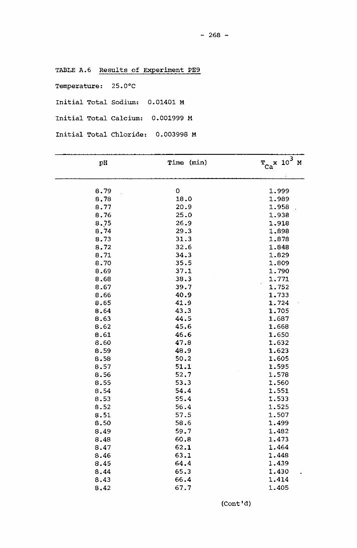
268
TABLE A.6 Results of Experiment PE9
Temperature: 25.0°C
Initial Total Sodium: 0.01401 M
Initial Total Calcium: 0.001999 M
Initial Total Chloride: 0.003998 M
PH Time (min) T x 10 Ca
8.79 0 1.9998.78 18.0 1.9898.77 20.9 1.9588.76 25.0 1.9388.75 26.9 1.9188.74 29.3 1.8988.73 31.3 1.8788.72 32.6 1.8488.71 34.3 1.8298.70 35.5 1.8098.69 37.1 1.7908.68 38.3 1.7718.67 39.7 1.7528.66 40.9 1.7338.65 41.9 1.7248.64 43.3 1.7058.63 44.5 1.6878.62 45.6 1.6688.61 46.6 1.6508.60 47.8 1.6328.59 48.9 1.6238.58 50.2 1.6058.57 51.1 1.5958.56 52.7 1.5788.55 53.3 1.5608.54 54.4 1.5518.53 55.4 1.5338.52 56.4 1.5258.51 57.5 1.5078.50 58.6 1.4998.49 59.7 1.4828.48 60.8 1.4738.47 62.1 1.4648.46 63.1 1.4488.45 64.4 1.4398.44 65.3 1.4308.43 66.4 1.4148.42 67.7 1.405
(Cont'd)
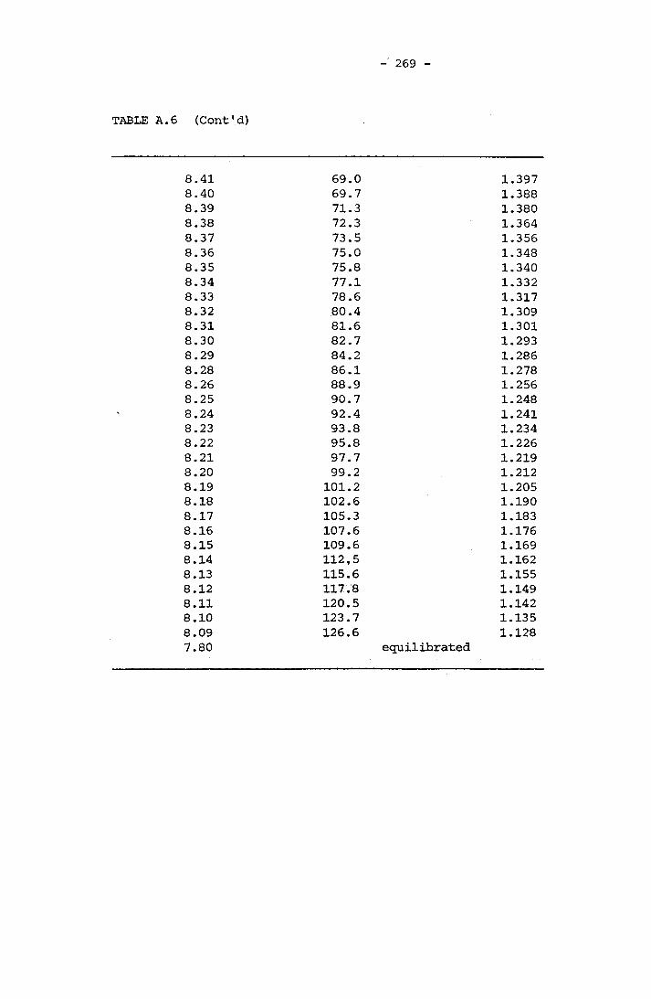
269
TABLE A.6 (Cont'd)
8.418.408.398.388.378.368.358.348.338.328.318.308.298.288.268.258.248.238.228.218.208.198.188.178.168.158.148.138.128.118.108.097.80
69.069.771.372.373.575.075.877.178.680.481.682.784.286.188.990.792.493.895.8 97.799.2
101.2 102.6 105.3107.6109.6112.5115.6 117.8120.5123.7126.6
1.3971.3881.3801.3641.3561.3481.3401.3321.3171.3091.3011.2931.2861.2781.2561.2481.2411.2341.2261.2191.2121.2051.1901.1831.1761.1691.1621.1551.1491.1421.1351.128
equilibrated
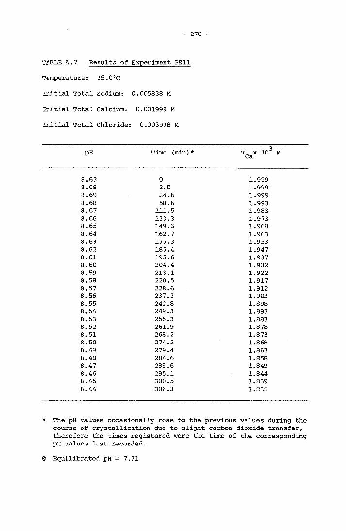
270
TABLE A.7 Results of Experiment PE11
Temperature: 25.0°CInitial Total Sodium: 0.005838 M
Initial Total Calcium: 0.001999 M
Initial Total Chloride: 0.003998 M
pH Time (min) * T x 103 MCa
8.63 0 1.9998.68 2.0 1.9998.69 24.6 1.9998.68 58.6 1.9938.67 111.5 1.9838.66 133.3 1.9738.65 149.3 1.9688.64 162.7 1.9638.63 175.3 1.9538.62 185.4 1.9478.61 195.6 1.9378.60 204.4 1.9328.59 213.1 1.9228.58 220.5 1.9178.57 228.6 1.9128.56 237.3 1.9038.55 242.8 1.8988.54 249.3 1.8938.53 255.3 1.8838.52 261.9 1.8788.51 268.2 1.8738.50 274.2 1.8688.49 279.4 1.8638.48 284.6 1.8588.47 289.6 1.8498.46 295.1 1.8448.45 300.5 1.8398.44 306.3 1.835
* The pH values occasionally rose to the previous values during the course of crystallization due to slight carbon dioxide transfer, therefore the times registered were the time of the corresponding pH values last recorded.
@ Equilibrated pH = 7.71
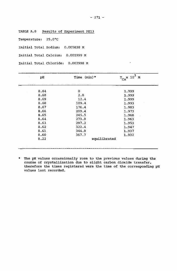
271
TABLE A.8 Results of Experiment PE13
Temperature: 25.0°CInitial Total Sodium: 0.005838 M
Initial Total Calcium: 0.001999 MInitial Total Chloride: 0.003998 M
PH Time (min) * T x 103 MCa
8.64 0 1.9998.68 2.0 1.9998.69 12.4 1.9998.68 109.4 1.9938.67 176.4 1.9838.66 209.4 1.9738.65 245.5 1.9688.64 273.8 1.9638.63 297.2 1.9538.62 322.4 1.9478.61 344.8 1.9378.608.22
367.7equilibrated
1.932
* The pH values occassionally rose to the previous values during the course of crystallization due to slight carbon dioxide transfer, therefore the times registered were the time of the corresponding pH values last recorded.
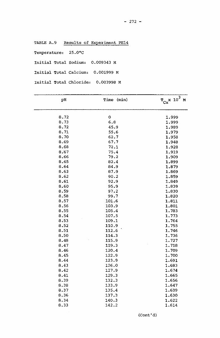
272
TABLE A.9 Results of Experiment PE14
Temperature: 25.0°C
Initial Total Sodium: 0.009343 M
Initial Total Calcium: 0.001999 M
Initial Total Chloride: 0.003998 M
PH Time (min) T x 10 Ca
8.72 0 1.9998.73 6.8 1.9998.72 45.9 1.9898.71 55.6 1.9798.70 62.7 1.9588.69 67.7 1.9488.68 72.1 1.9288.67 75.4 1.9198.66 79.2 1.9098.65 82.4 1.8998.64 84.9 1.8798.63 87.9 1.8698.62 90.2 1.8598.61 92.9 1.8498.60 95.9 1.8398.59 97.2 1.8308.58 99.7 1.8208.57 101.6 1.8118.56 103.9 1.8018.55 105.4 1.7838.54 107.5 1.7738.53 109.1 1.7648.52 110.9 1.7558.51 112.6 1.7468.50 114.3 1.7368.48 115.9 1.7278.47 119.3 1.7188.46 120.4 1.7098.45 122.9 1.7008.44 123.9 1.6918.43 126.0 1.6838.42 127.9 1.6748.41 129.3 1.6658.39 132.3 1.6568.38 133.9 1.6478.37 135.4 1.6398.36 137.3 1.6308.34 140.3 1.6228.33 142.2 1.614
(Cont'd)
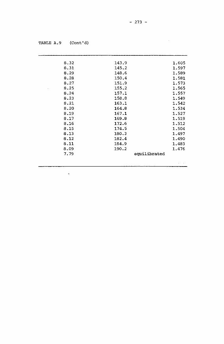
273
TABLE A.9 (Cont'd)
8.328.318.298.288.278.258.248.238.218.208.198.178.168.158.138.128.118.097.79
143.9145.2148.6150.4151.9155.2157.1158.8163.1164.8167.1169.8172.6174.5180.3182.4184.9190.2
1.6051.5971.5891.5811.5731.5651.5571.5491.5421.5341.5271.5191.5121.5041.4971.4901.4831.476
equilibrated

274
TABLE A.10 Results of Experiment PE15
Temperature: 25.0°C
Initial Total Sodium: 0.01185 M
Initial Total Calcium: 0.001999 M
Initial Total Chloride: 0.003998 M
PH Time (min) T x 10 Ca
8.85 0 1.9998.84 5.4 1.9888.83 7.6 1.9678.82 9.0 1.9378.81 10.2 1.9178.80 11.2 1.8968.79 12.0 1.8778.78 12.8 1.8578.77 13.6 1.8378.76 14.2 1.8178.75 14.8 1.8008.74 15.4 1.7798.73 16.0 1.7598.72 16.5 1.7508.71 17.0 1.7308.70 17.5 1.7128.69 18.0 1.7028.68 18.5 1.6838.67 15.9 1.6648.66 19.4 1.6558.65 19.8 1.6378.64 20.4 1.6278.63 20.7 1.6098.62 21.3 1.6008.61 21.6 1.5828.60 22.0 1.5738.59 22.4 1.5648.58 22.8 1.5468.57 23.2 1.5378.56 23.6 1.5288.55 24.0 1.5108.54 24.4 1.5018.53 24.9 1.4928.52 25.3 1.4838.51 25.6 1.4748.50 26.0 1.4578.49 26.4 1.4498.48 26.8 1.4408.47 27.2 1.4328.46 27.6 1.423
(Cont'd)
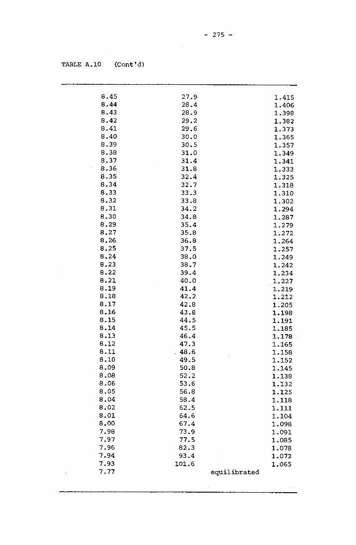
275
TABLE A.10 (Cont'd)
8.458.448.438.428.418.408.398.388.378.368.358.348.338.328.318.308.298.278.268.258.248.238.228.218.198.188.178.168.158.148.138.128.118.108.098.088.068.058.048.028.018.007.987.977.967.947.937.77
27.928.428.929.229.630.030.531.031.4 31.832.432.733.333.834.234.835.435.836.837.538.038.739.440.041.442.242.843.844.545.546.447.348.649.550.852.253.656.858.462.564.667.473.977.582.393.4
101.6
1.4151.4061.3981.3821.3731.3651.3571.3491.3411.3331.3251.3181.3101.3021.2941.2871.2791.2721.2641.2571.2491.2421.2341.2271.2191.2121.2051.1981.1911.1851.1781.1651.1581.1521.1451.1381.1321.1251.1181.1111.1041.0981.0911.0851.0781.0721.065
equilibrated

276
TABLE A.11 Results of Experiment PE16
Temperature: 25.0°C
Initial Total Sodium: 0.01231 M
Initial Total Calcium: 0.001999 M
Initial Total Chloride: 0.003998 M
PH Time (min) T x 10 Ca
9.03 0 1.9999.02 5.0 1.9789.01 6.3 1.9479.00 7.1 1.9168.99 7.8 1.8858.98 8.6 1.8548.97 9.1 1.8248.96 9.6 1.7948.95 10.2 1.7648.94 10.6 1.7348.93 11.2 1.7048.92 11.6 1.6858.91 11.9 1.6558.90 12.3 1.6368.89 12.8 1.6078.88 13.1 1.5878.87 13.5 1.5598.86 13.9 1.5408.85 14.3 1.5218.84 14.6 1.5028.83 14.9 1.4838.82 15.3 1.4648.81 15.6 1.4468.80 16.0 1.4278.79 16.3 1.4098.78 16.7 1.3918.77 17.0 1.3738.76 17.3 1.3558.75 17.7 1.3378.74 18.0 1.3208.73 18.4 1.3028.72 18.8 1.2938.71 19.0 1.2768.70 19.4 1.2588.69 19.8 1.2508.67 20.4 1.2248.66 20.7 1.2078.65 21.1 1.1998.64 21.4 1.1828.63 22.0 1.1738.62 22.3 1.157
(Cont'd)
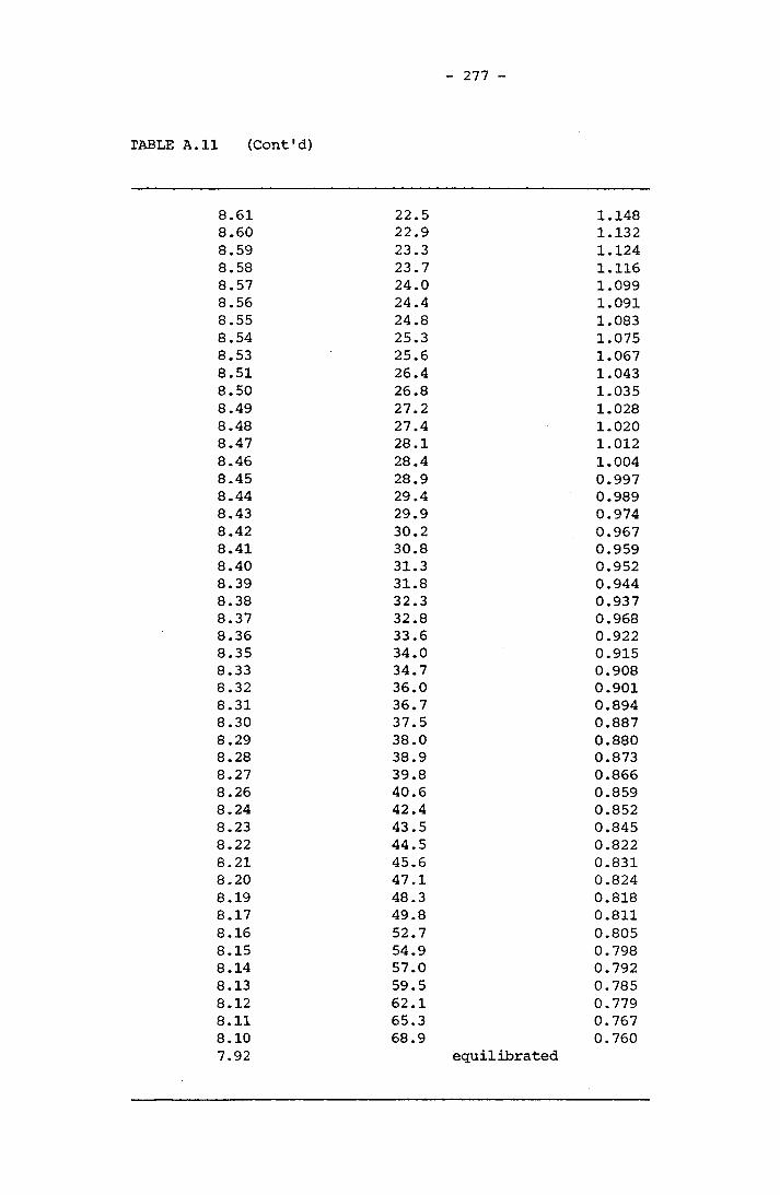
277
TABLE A.11 (Cont'd)
8.61 22.58.60 22.98.59 23.38.58 23.78.57 24.08.56 24.48.55 24.88.54 25.38.53 25.68.51 26.48.50 26.88.49 27.28.48 27.48.47 28.18.46 28.48.45 28.98.44 29.48.43 29.98.42 30.28.41 30.88.40 31.38.39 31.88.38 32.38.37 32.88.36 33.68.35 34.08.33 34.78.32 36.08.31 36.78.30 37.58.29 38.08.28 38.98.27 39.88.26 40.68.24 42.48.23 43.58.22 44.58.21 45.68.20 47.18.19 48.38.17 49.88.16 52.78.15 54.98.14 57.08.13 59.58.12 62.18.11 65.38.10 68.97.92
1.1481.1321.1241.1161.0991.0911.0831.0751.0671.0431.0351.0281.0201.0121.0040.9970.9890.9740.9670.9590.9520.9440.9370.9680.9220.9150.9080.9010.8940.8870.8800.8730.8660.8590.8520.8450.8220.8310.8240.8180.8110.8050.7980.7920.7850.7790.7670.760
equilibrated

278
TABLE A.12 Results of Experiment PE18
Temperature: 25.0°C
Initial Total Sodium: 0.01167 M
Initial Total Calcium: 0.001999 M
Initial Total Magnesium: 0.002001 M
Initial Total Chloride: 0.007998 M
pH Time (min) T x 10 Ca
8.45 0 1.9998.44 34.6 1.9858.43 42.9 1.9578.41 49.6 1.9168.40 56.0 1.9028.39 64.7 1.8758.38 68.3 1.8618.37 72.8 1.8348.36 75.9 1.8218.35 79.2 1.8078.34 82.7 1.7808.33 86.0 1.7678.32 89.1 1.7548.31 92.9 1.7278.30 96.1 1.7148.29 99.3 1.7008.28 102.7 1.6878.27 106.0 1.6618.26 109.9 1.6488.25 112.6 1.6358.24 116.1 1.6228.23 119.0 1.6098.22 122.4 1.5968.21 125.4 1.5718.20 127.8 1.5588.19 131.9 1.5458.18 134.8 1.5338.17 138.4 1.5208.16 141.8 1.5078.15 145.4 1.4958.14 148.8 1.4828.13 152.9 1.4708.12 156.7 1.4578.11 160.4 1.4458.10 164.5 1.4338.09 168.6 1.420
(Cont'd)
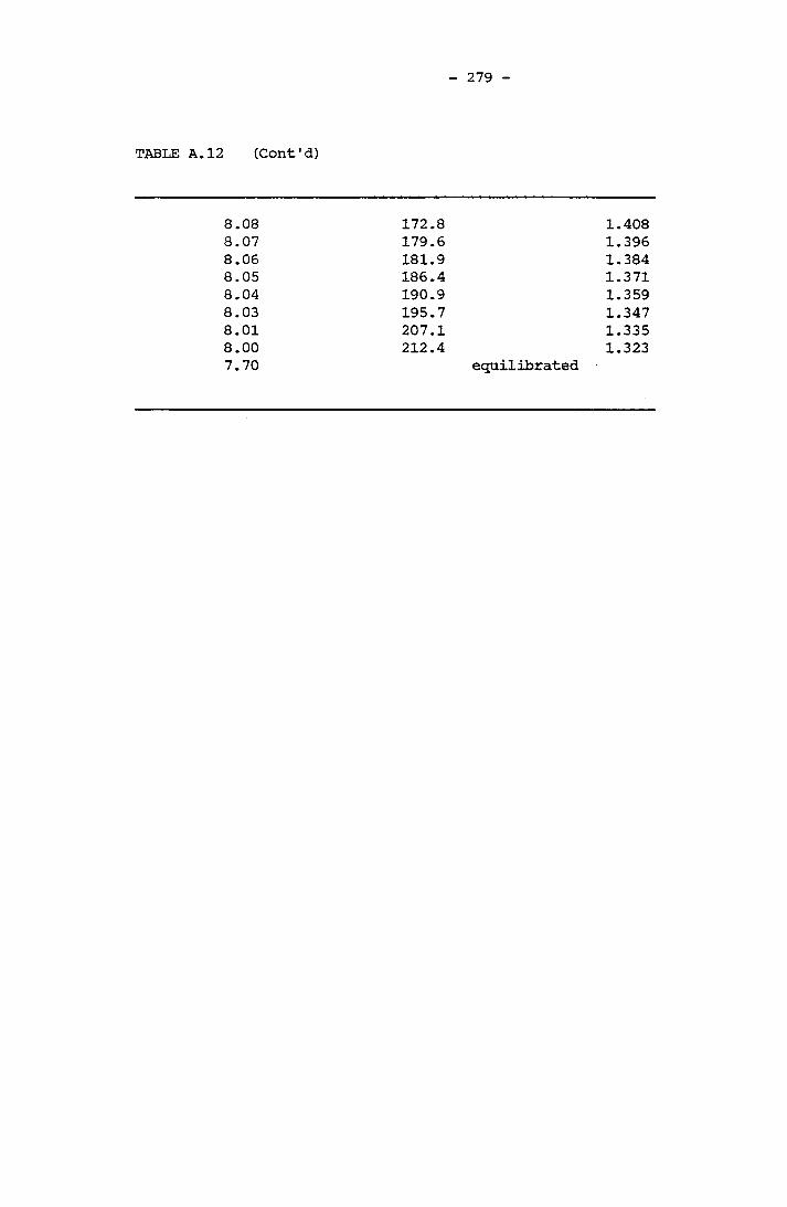
279
TABLE A.12 (Cont'd)
8.08 172.8 1.4088.07 179.6 1.3968.06 181.9 1.3848.05 186.4 1.3718.04 190.9 1.3598.03 195.7 1.3478.01 207.1 1.3358.007.70
212.4 1.323equilibrated
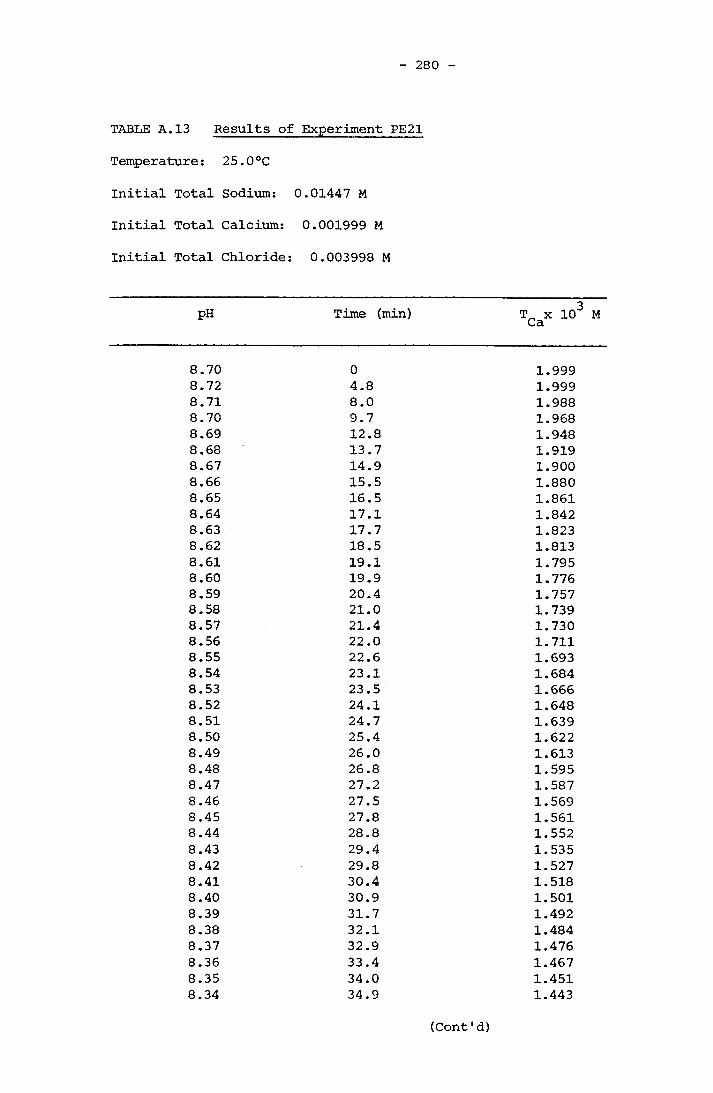
280
TABLE A.13 Results of Experiment PE21
Temperature: 25.0°C
Initial Total Sodium: 0.01447 M
Initial Total Calcium: 0.001999 M
Initial Total Chloride: 0.003998 M
PH Time (min) T x 10 Ca
8.70 0 1.9998.72 4.8 1.9998.71 8.0 1.9888.70 9.7 1.9688.69 12.8 1.9488.68 13.7 1.9198.67 14.9 1.9008.66 15.5 1.8808.65 16.5 1.8618.64 17.1 1.8428.63 17.7 1.8238.62 18.5 1.8138.61 19.1 1.7958.60 19.9 1.7768.59 20.4 1.7578.58 21.0 1.7398.57 21.4 1.7308.56 22.0 1.7118.55 22.6 1.6938.54 23.1 1.6848.53 23.5 1.6668.52 24.1 1.6488.51 24.7 1.6398.50 25.4 1.6228.49 26.0 1.6138.48 26.8 1.5958.47 27.2 1.5878.46 27.5 1.5698.45 27.8 1.5618.44 28.8 1.5528.43 29.4 1.5358.42 29.8 1.5278.41 30.4 1.5188.40 30.9 1.5018.39 31.7 1.4928.38 32.1 1.4848.37 32.9 1.4768.36 33.4 1.4678.35 34.0 1.4518.34 34.9 1.443
(Cont'd)
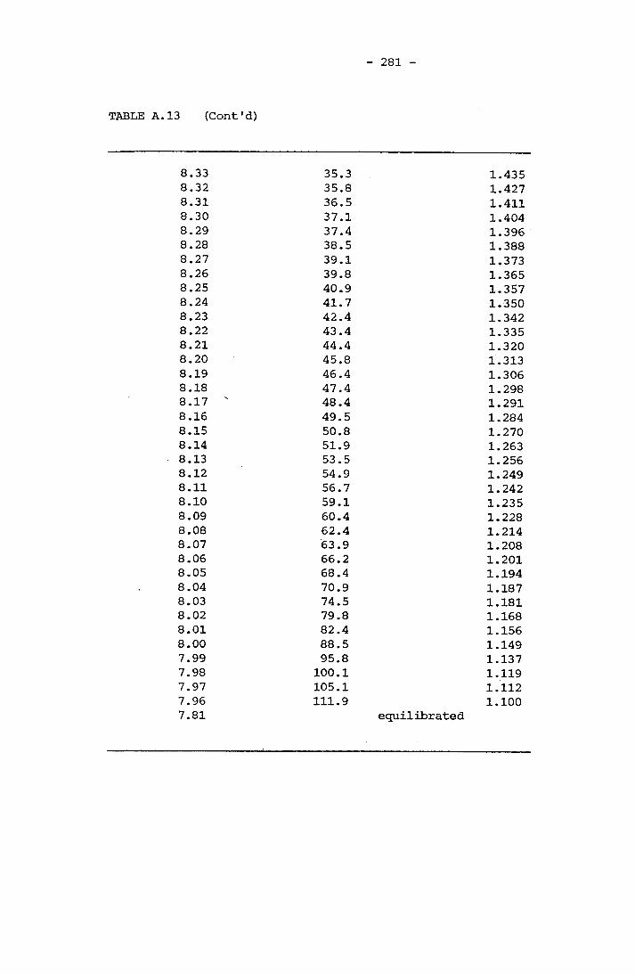
281
TABLE A.13 (Cont'd)
8.338.328.318.308.298.288.278.268.258.248.238.228.218.208.198.188.178.168.158.148.138.128.118.108.098.088.078.068.058.048.038.028.018.007.997.987.977.967.81
35.335.8 36.537.137.438.539.139.840.941.742.443.444.445.846.447.448.449.550.851.953.554.956.759.160.462.463.966.268.470.974.579.882.488.595.8 100.1 105.1 111.9
1.4351.4271.4111.4041.3961.3881.3731.3651.3571.3501.3421.3351.3201.3131.3061.2981.2911.2841.2701.2631.2561.2491.2421.2351.2281.2141.2081.2011.1941.1871.1811.1681.1561.1491.1371.1191.1121.100
equilibrated
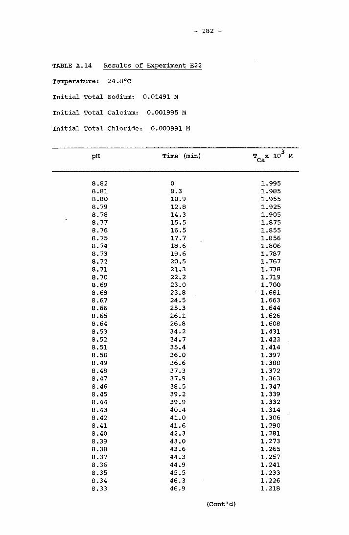
282
TABLE A.14 Results of Experiment E22
Temperature: 24.8°C
Initial Total Sodium: 0.01491 M
Initial Total Calcium: 0.001995 M
Initial Total Chloride: 0.003991 M
PH Time (min) T x 10' Ca
8.82 0 1.9958.81 8.3 1.9858.80 10.9 1.9558.79 12.8 1.9258.78 14.3 1.9058.77 15.5 1.8758.76 16.5 1.8558.75 17.7 1.8568.74 18.6 1.8068.73 19.6 1.7878.72 20.5 1.7678.71 21.3 1.7388.70 22.2 1.7198.69 23.0 1.7008.68 23.8 1.6818.67 24.5 1.6638.66 25.3 1.6448.65 26.1 1.6268.64 26.8 1.6088.53 34.2 1.4318.52 34.7 1.4228.51 35.4 1.4148.50 36.0 1.3978.49 36.6 1.3888.48 37.3 1.3728.47 37.9 1.3638.46 38.5 1.3478.45 39.2 1.3398.44 39.9 1.3328.43 40.4 1.3148.42 41.0 1.3068.41 41.6 1.2908.40 42.3 1.2818.39 43.0 1.2738.38 43.6 1.2658.37 44.3 1.2578.36 44.9 1.2418.35 45.5 1.2338.34 46.3 1.2268.33 46.9 1.218
(Cont'd)

283
TABLE A.14 (Cont'd)
8.32 47.68.31 48.48.30 49.08.29 49.78.28 50.58.27 51.28.26 52.08.25 52.78.247.50
53.4
1.2031.1951.1881.1801.1651.1581.1511.1431.136
equilibrated
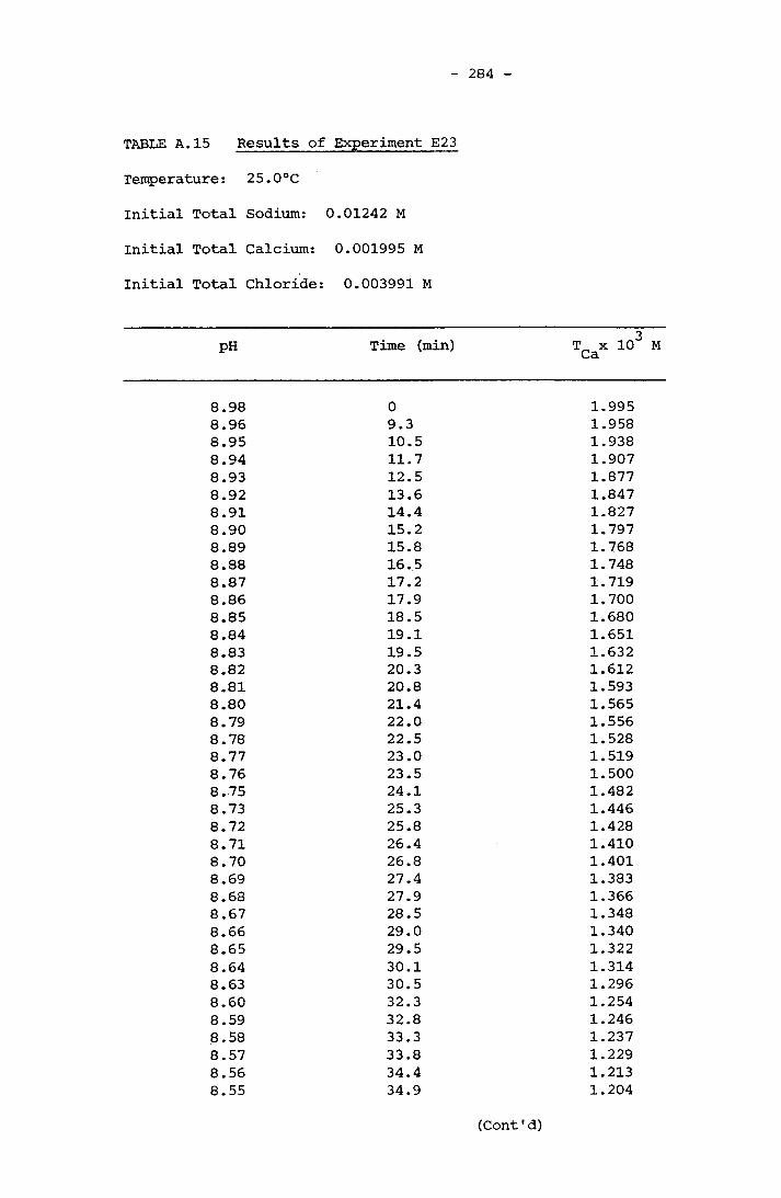
284
TABLE A.15 Results of Experiment E23
Temperature: 25.0°C
Initial Total Sodium: 0.01242 M
Initial Total Calcium: 0.001995 M
Initial Total Chloride: 0.003991 M
PH Time (min) T x 10 Ca
8.98 0 1.9958.96 9.3 1.9588.95 10.5 1.9388.94 11.7 1.9078.93 12.5 1.8778.92 13.6 1.8478.91 14.4 1.8278.90 15.2 1.7978.89 15.8 1.7688.88 16.5 1.7488.87 17.2 1.7198.86 17.9 1.7008.85 18.5 1.6808.84 19.1 1.6518.83 19.5 1.6328.82 20.3 1.6128.81 20.8 1.5938.80 21.4 1.5658.79 22.0 1.5568.78 22.5 1.5288.77 23.0 1.5198.76 23.5 1.5008.75 24.1 1.4828.73 25.3 1.4468.72 25.8 1.4288.71 26.4 1.4108.70 26.8 1.4018.69 27.4 1.3838.68 27.9 1.3668.67 28.5 1.3488.66 29.0 1.3408.65 29.5 1.3228.64 30.1 1.3148.63 30.5 1.2968.60 32.3 1.2548.59 32.8 1.2468.58 33.3 1.2378.57 33.8 1.2298.56 34.4 1.2138.55 34.9 1.204
(Cont1d)
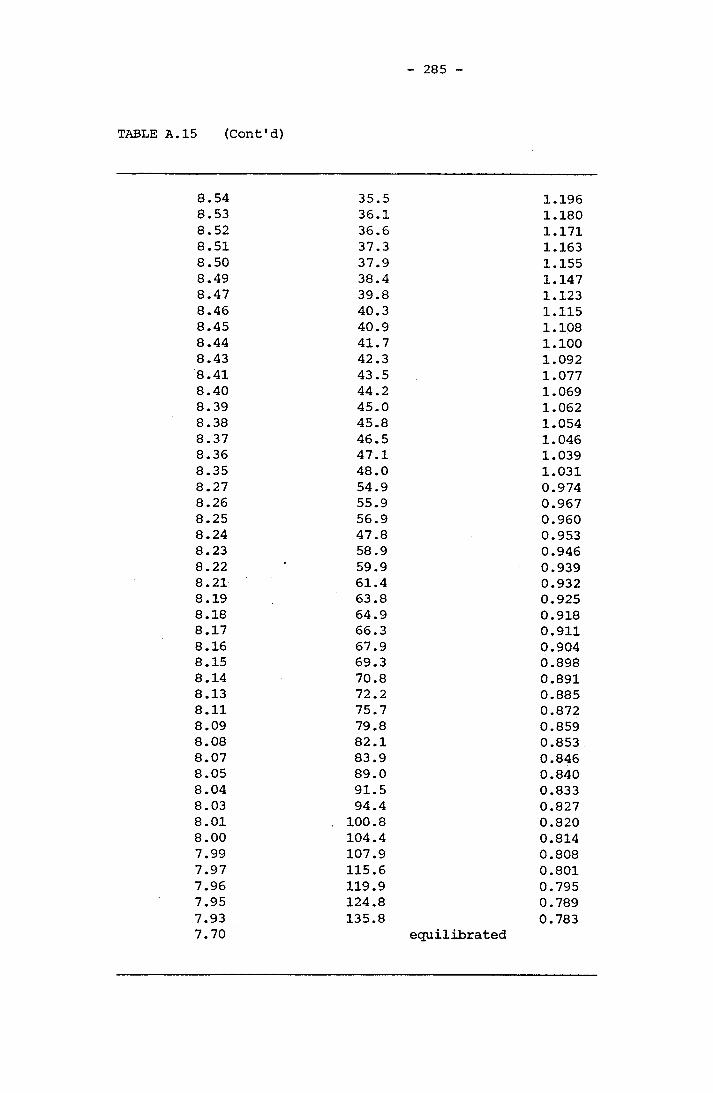
285
TABLE A.15 (Cont'd)
8.548.538.528.518.508.498.478.468.458.448.438.418.408.398.388.378.368.358.278.268.258.248.238.228.218.198.188.178.168.158.148.138.118.098.088.078.058.048.038.018.007.997.977.967.957.937.70
35.536.136.637.3 37.938.439.840.340.941.742.343.544.245.045.846.547.148.054.955.956.947.858.959.961.463.864.966.367.969.3 70.872.275.779.882.183.9 89.091.594.4
100.8 104.4107.9 115.6119.9124.8135.8
1.1961.1801.1711.1631.1551.1471.1231.1151.1081.1001.0921.0771.0691.0621.0541.0461.0391.0310.9740.9670.9600.9530.9460.9390.9320.9250.9180.9110.9040.8980.8910.8850.8720.8590.8530.8460.8400.8330.8270.8200.8140.8080.8010.7950.7890.783
equilibrated
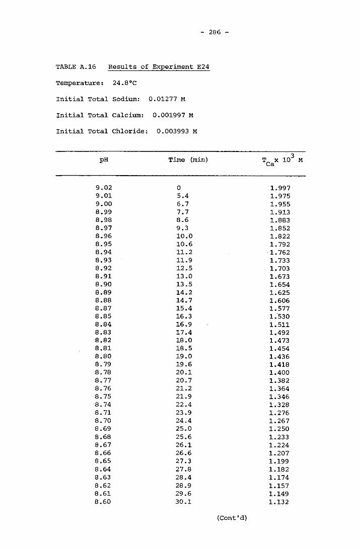
286
TABLE A.16 Results of Experiment E24
Temperature: 24.8°C
Initial Total Sodium: 0.01277 M
Initial Total Calcium: 0.001997 M
Initial Total Chloride: 0.003993 M
pH Time (min) T x 10 Ca
9.02 0 1.9979.01 5.4 1.9759.00 6.7 1.9558.99 7.7 1.9138.98 8.6 1.8838.97 9.3 1.8528.96 10.0 1.8228.95 10.6 1.7928.94 11.2 1.7628.93 11.9 1.7338.92 12.5 1.7038.91 13.0 1.6738.90 13.5 1.6548.89 14.2 1.6258.88 14.7 1.6068.87 15.4 1.5778.85 16.3 1.5308.84 16.9 1.5118.83 17.4 1.4928.82 18.0 1.4738.81 18.5 1.4548.80 19.0 1.4368.79 19.6 1.4188.78 20.1 1.4008.77 20.7 1.3828.76 21.2 1.3648.75 21.9 1.3468.74 22.4 1.3288.71 23.9 1.2768.70 24.4 1.2678.69 25.0 1.2508.68 25.6 1.2338.67 26.1 1.2248.66 26.6 1.2078.65 27.3 1.1998.64 27.8 1.1828.63 28.4 1.1748.62 28.9 1.1578.61 29.6 1.1498.60 30.1 1.132
(Cont'd)
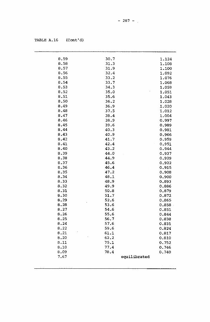
287
TABLE A.16 (Cont'd)
8.59 30.78.58 31.38.57 31.98.56 32.48.55 33.28.54 33.78.53 34.38.52 35.08.51 35.68.50 36.28.49 36.98.48 37.58.47 38.48.46 38.98.45 39.68.44 40.38.43 40.98.42 41.78.41 42.48.40 43.28.39 44.08.38 44.98.37 45.68.36 46.48.35 47.28.34 48.18.33 48.98.32 49.98.31 50.88.30 51.78.29 52.68.28 53.68.27 54.68.26 55.68.25 56.78.24 57.68.22 59.68.21 61.18.20 62.28.11 75.18.10 77.48.09 78.47.67
1.1241.1081.1001.0921.0761.0681.0591.0511.0431.0281.0201.0121.0040.9970.9890.9810.9660.9590.9510.9440.9370.9290.9220.9150.9080.9000.8930.8860.8790.8720.8650.8580.8510.8440.8380.8310.8240.8170.8100.7520.7460.740
equilibrated

288
APPENDIX B
PHOTOMICROGRAPHS OF CRYSTALS FROM SPONTANEOUS CRYSTALLIZATION EXPERIMENTS
Some of the final crystal products from the spontaneous crystalli
zation experiments (Chapter 4) were photographed under light transmitting microscope (Zeiss Universal microscope, School of Mining) and scanning electron microscope (ISI 100A, School of Textile Technology). Sam
ples photographed under the scanning electron microscope were coated with gold to form a conductive coating.
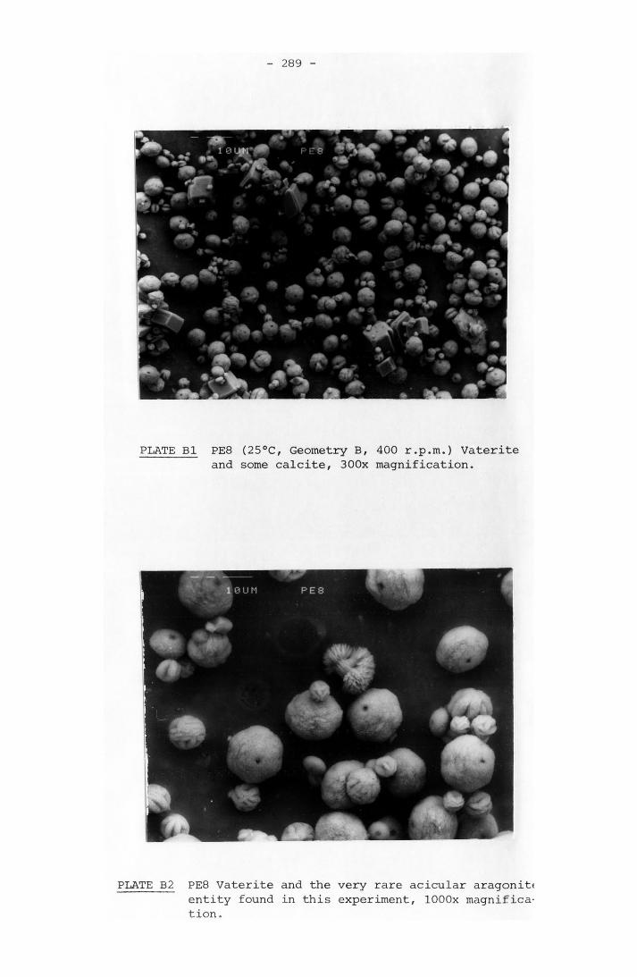
289
PLATE Bl PE8 (25°C, Geometry B, 400 r.p.m.) Vaterite and some calcite, 300x magnification.
PLATE B2 PE8 Vaterite and the very rare acicular aragonit< entity found in this experiment, lOOOx magnification.
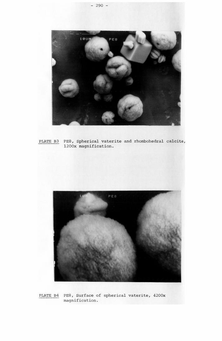
290
PLATE B3 PE8, Spherical vaterite and rhombohedral calcite, 1200x magnification.
PLATE B4 PE8, Surface of spherical vaterite, 4200x magnification.
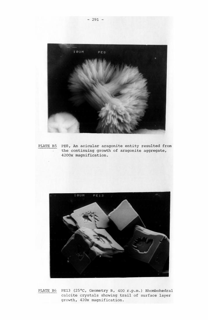
291
PLATE B5 PE8, An acicular aragonite entity resulted from the continuing growth of aragonite aggregate, 4200x magnification.
PLATE B6 PE13 (25°C, Geometry B, 400 r.p.m.) Rhombohedral calcite crystals showing trail of surface layer growth, 420x magnification.
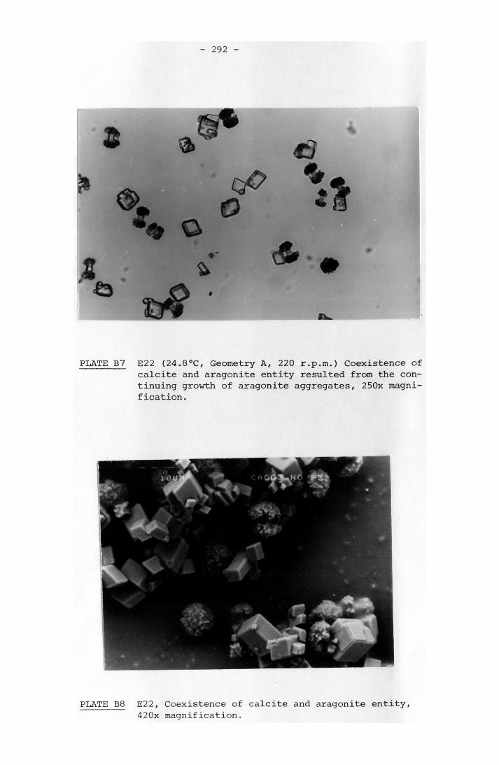
292
PLATE B7 E22 (24.8°C, Geometry A, 220 r.p.m.) Coexistence of calcite and aragonite entity resulted from the continuing growth of aragonite aggregates, 250x magnification.
PLATE B8 E22, Coexistence of calcite and aragonite entity, 420x magnification.
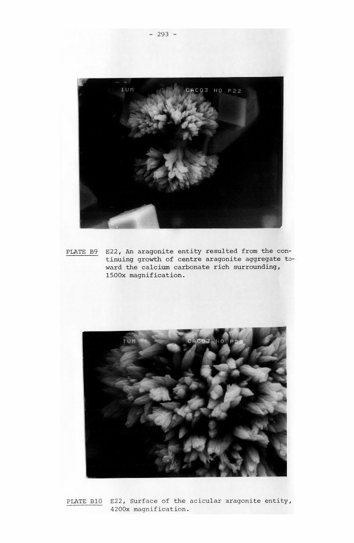
293
PLATE B9 E22, An aragonite entity resulted from the continuing growth of centre aragonite aggregate to- ward the calcium carbonate rich surrounding, 1500x magnification.
PLATE BIO E22, Surface of the acicular aragonite entity, 4200x magnification.
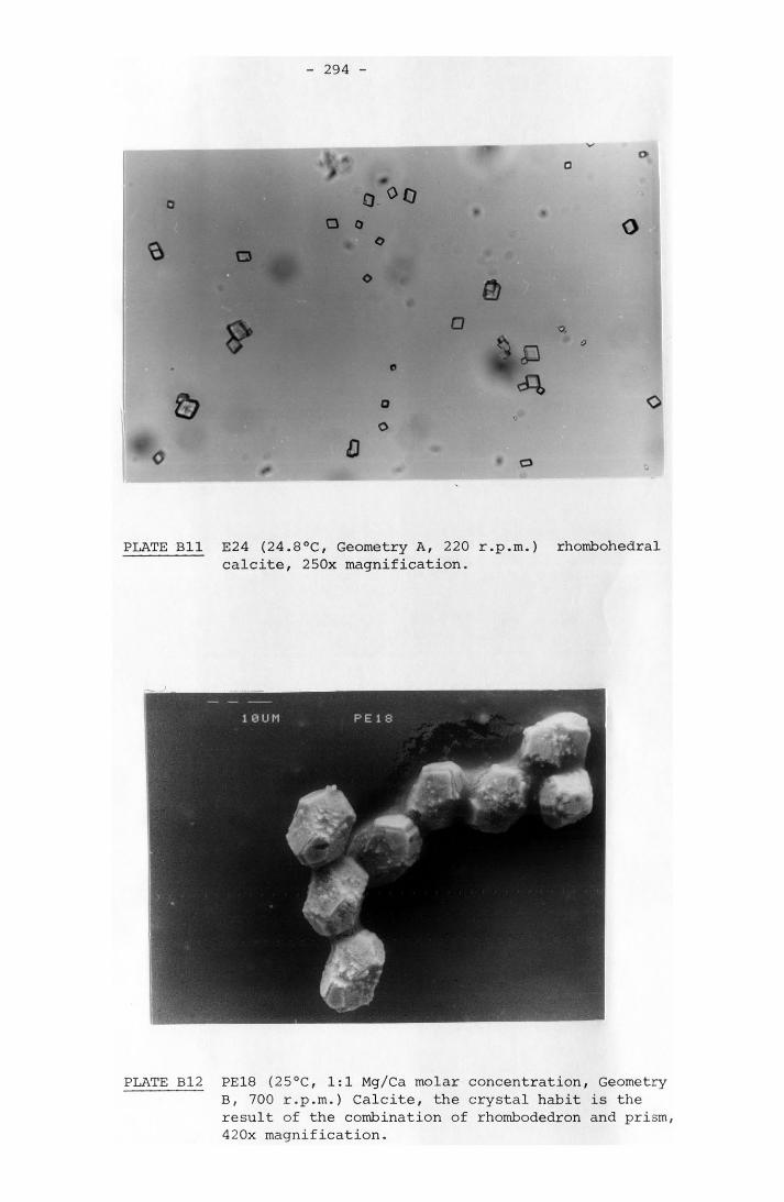
294
PLATE Bll E24 (24.8°C, Geometry A, 220 r.p.m.) rhombohedral calcite, 250x magnification.
PLATE B12 PE18 (25°C, 1:1 Mg/Ca molar concentration, Geometry B, 700 r.p.m.) Calcite, the crystal habit is the result of the combination of rhombodedron and prism, 420x magnification.
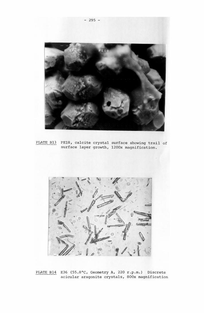
295
PLATE B13 PE18, calcite crystal surface showing trail ofsurface layer growth, 1200x magnification.
PLATE B14 E36 (55.8°C, Geometry A, 220 r.p.m.) Discreteacicular aragonite crystals, 800x magnification
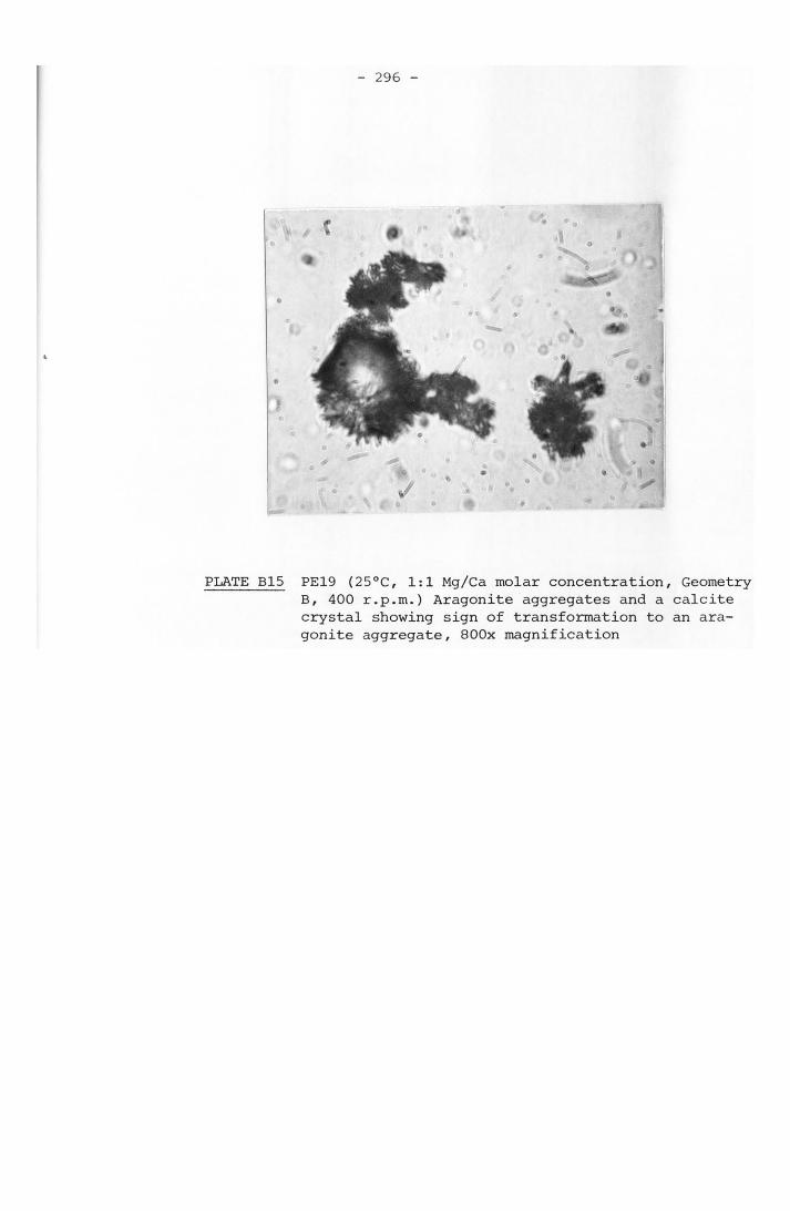
296
$ *
PLATE B15 PE19 (25°C, 1:1 Mg/Ca molar concentration, Geometry B, 400 r.p.m.) Aragonite aggregates and a calcite crystal showing sign of transformation to an aragonite aggregate, 800x magnification

297
APPENDIX C
GRAPHS OF THE SPONTANEOUS CRYSTALLIZATION EXPERIMENTS - THE CALCULATION OF THE OVERALL GROWTH RATE CONSTANTS
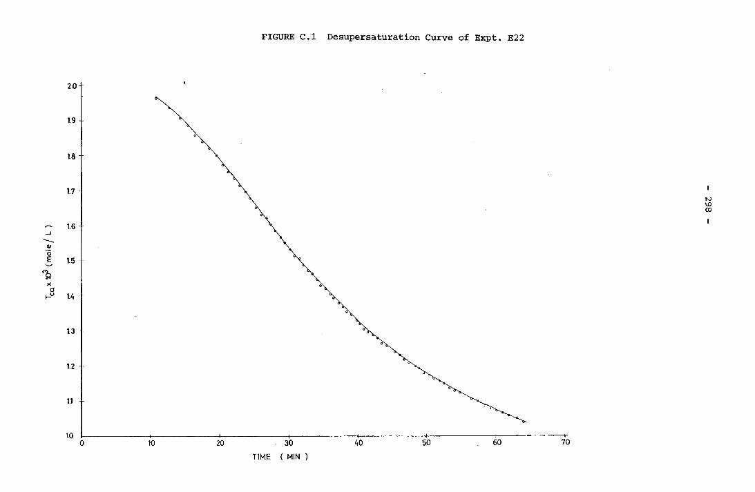
FIGURE C.l Desupersaturation Curve of Expt. E22298
TIME ( MIN

FIGURE C.2 Overall Growth Rate Constant of Expt. E22 Determined from Size Consideration
299
_L O-- CO
(■jU
iouiw
-i/spoO
gOlx^
X
;c)x108(mole2/L2)
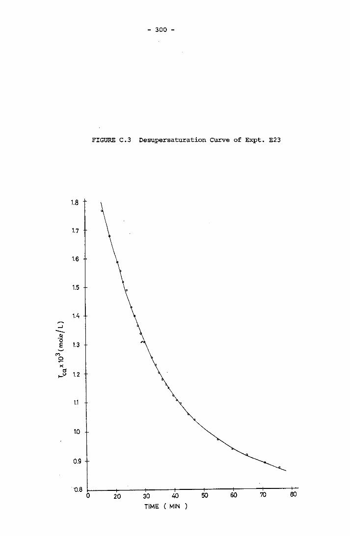
300
FIGURE C.3 Desupersaturation Curve of Expt. E23
y 1.2
TIME ( MIN )
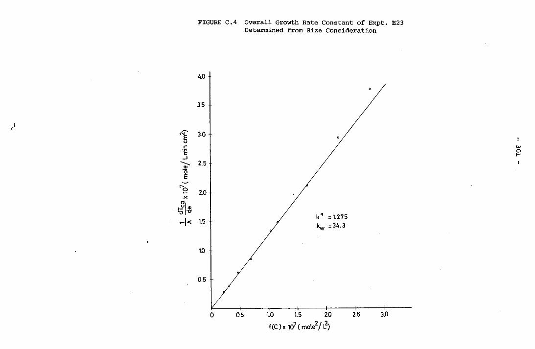
FIGURE C.4 Overall Growth Rate Constant of Expt. E23 Determined from Size Consideration
301
ep V
, C ) x 10' ( mole2/ L2)
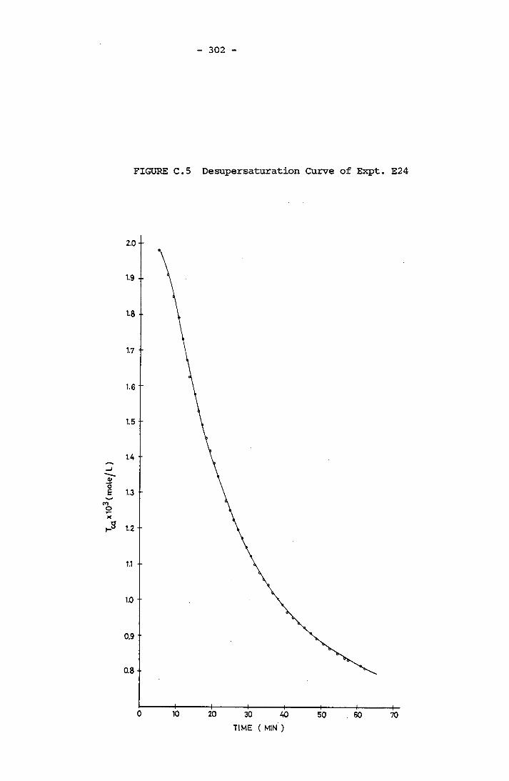
302
FIGURE C.5 Desupersaturation Curve of Expt. E24
TIME ( MIN )

FIGURE C .6 Overall Growth Rate Constant of Expt. E24 Determined from Size Determination
303
(C) x 10 (moley ̂2 )
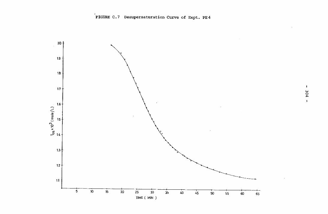
FIGURE C.7 Desupersaturation Curve of Expt, PE 4304
ME ( MIN
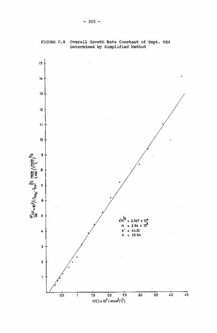
15
14
13
12
11
10
9
8
7
6
5
4
3
2
1
305
JURE C. 8 Overall Growth Rate Constant of Expt. PE4 Determined by Simplified Method
2.927 x 10'2.94 x itf
22.84

306
FIGURE C.9 Overall Growth Rate Constant of Expt. PE4 Determined by Size Consideration
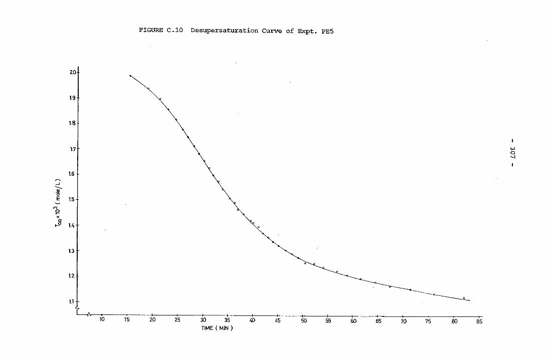
FIGURE C.10 Desupersaturation Curve of Expt. PE5307
IME ( MIN
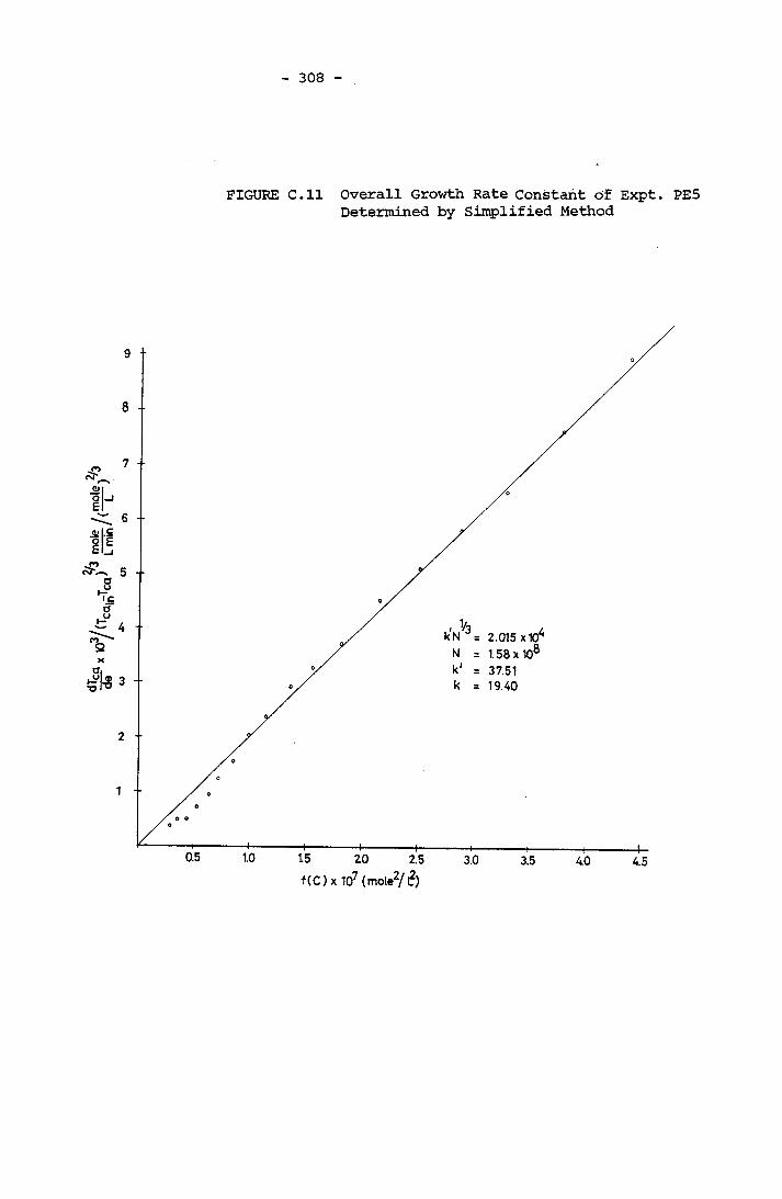
308
FIGURE C.ll Overall Growth Rate Constant of Expt. PE5 Determined by Simplified Method
2.015 x 10 1.58 x 10®
k = 19.40
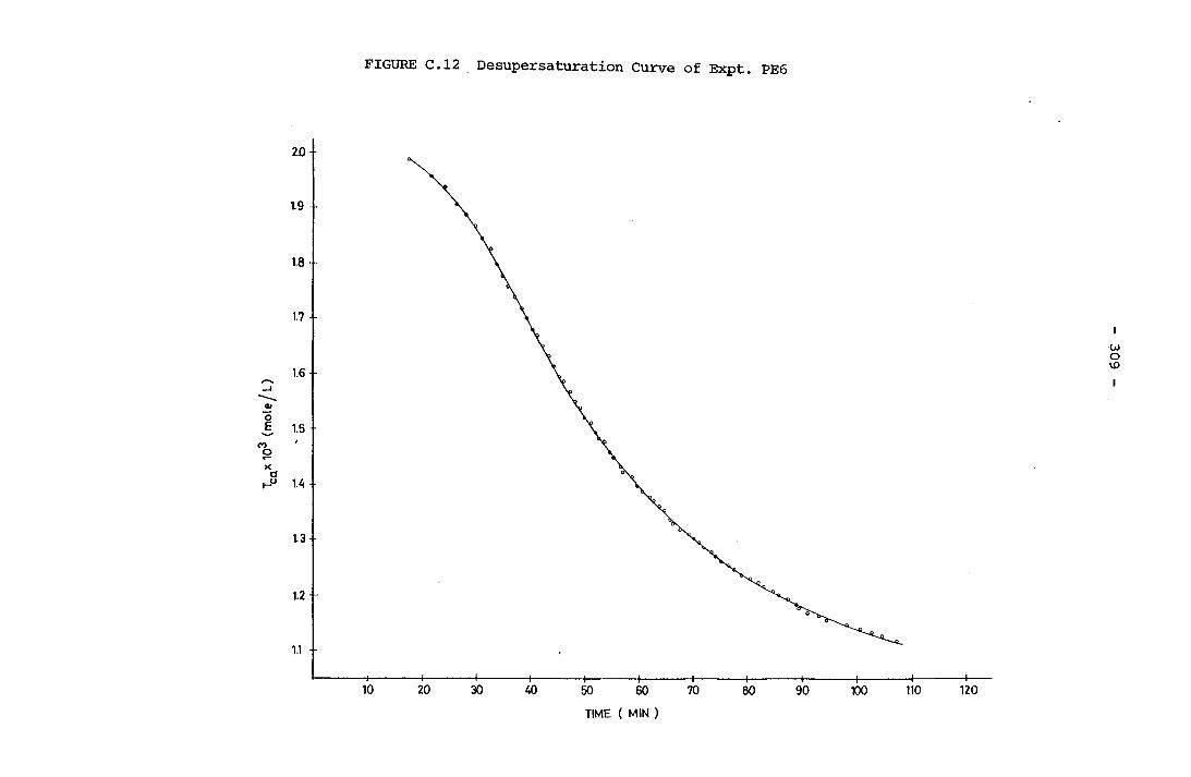
FIGURE C .12 Desupersaturation Curve of Expt. PE6309
-8 i
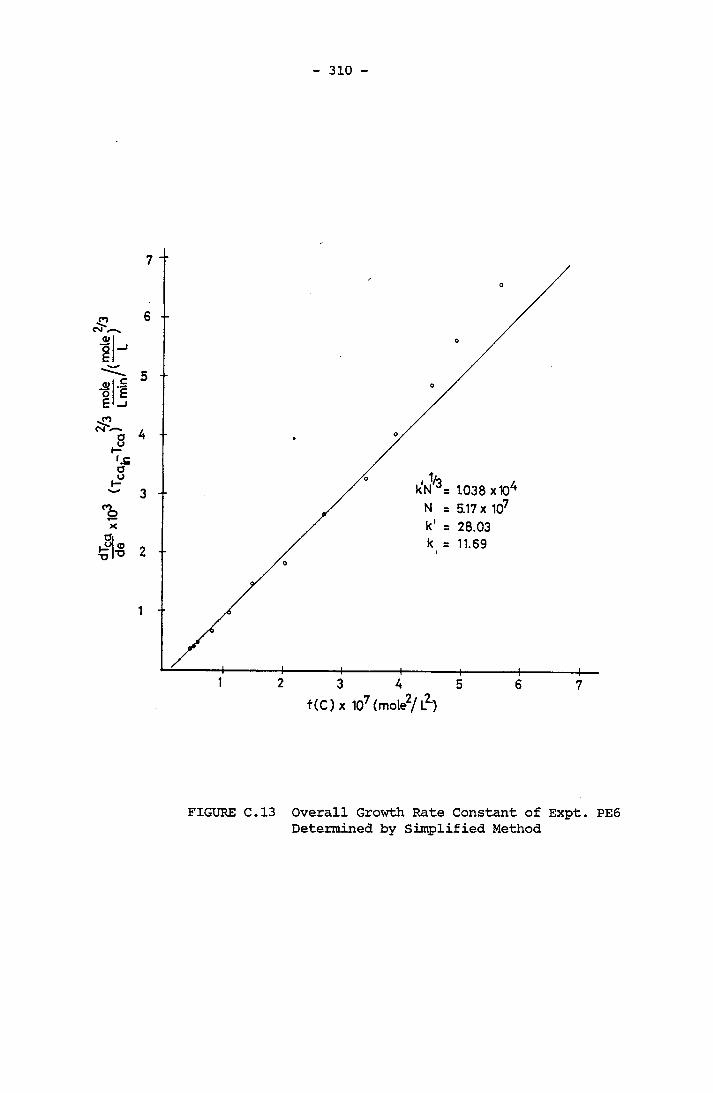
310
kN J= 1.038 xX) N = 5.17 x 10⁷ k' = 28.03 k = 11.69
FIGURE C.13 Overall Growth Rate Constant of Expt. PE6 Determined by Simplified Method
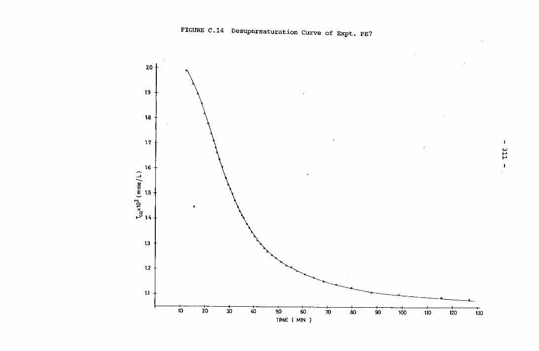
FIGURE C.14 Desupersaturation Curve of Expt. PE7311
++
up( 1 / d|O
UJ ) £
0l*
D3l
H--------------------------(-
tNI
r-ocvl
2
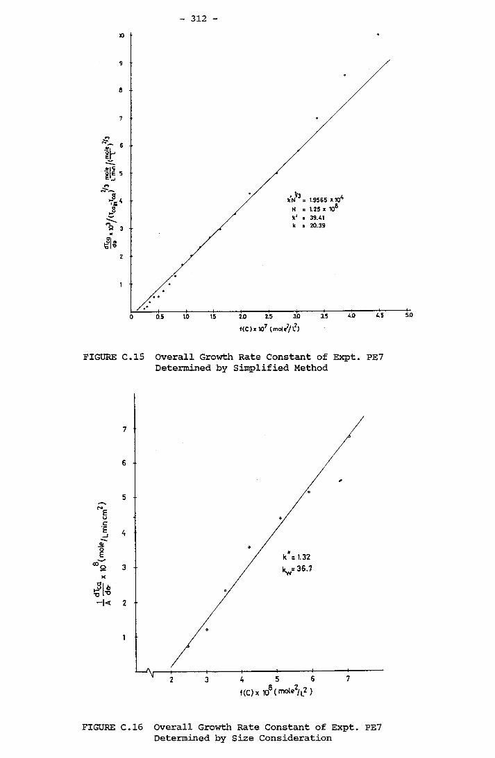
312
kN 3 = 1.9565 * 10A
20 2.5 3.0t(C) x 107 (mole2/12)
FIGURE C.15 Overall Growth Rate Constant of Expt. PE7 Determined by Simplified Method
H< 2
FIGURE C.16 Overall Growth Rate Constant of Expt. PE7 Determined by Size Consideration
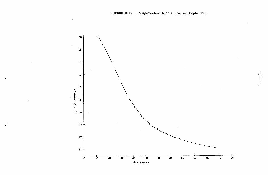
FIGURE C.17 Desupersaturation Curve of Expt. PE8313
ME ( M!N

314
FIGURE C.18 Overall Growth Rate Constant of Expt. PE8 Determined by Simplified Method

315
FIGURE C.19 Overall Growth Rate Constant of Expt. PE8 Determined by Size Consideration
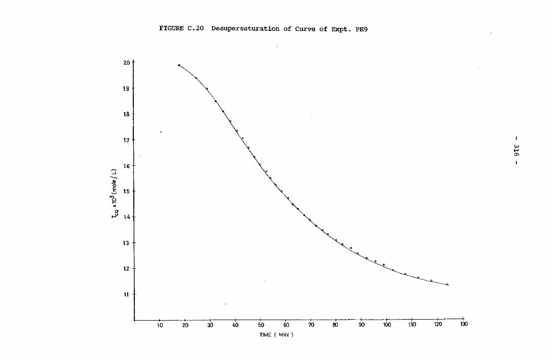
FIGURE C .20 Desupersaturation of Curve of Expt. PE9316
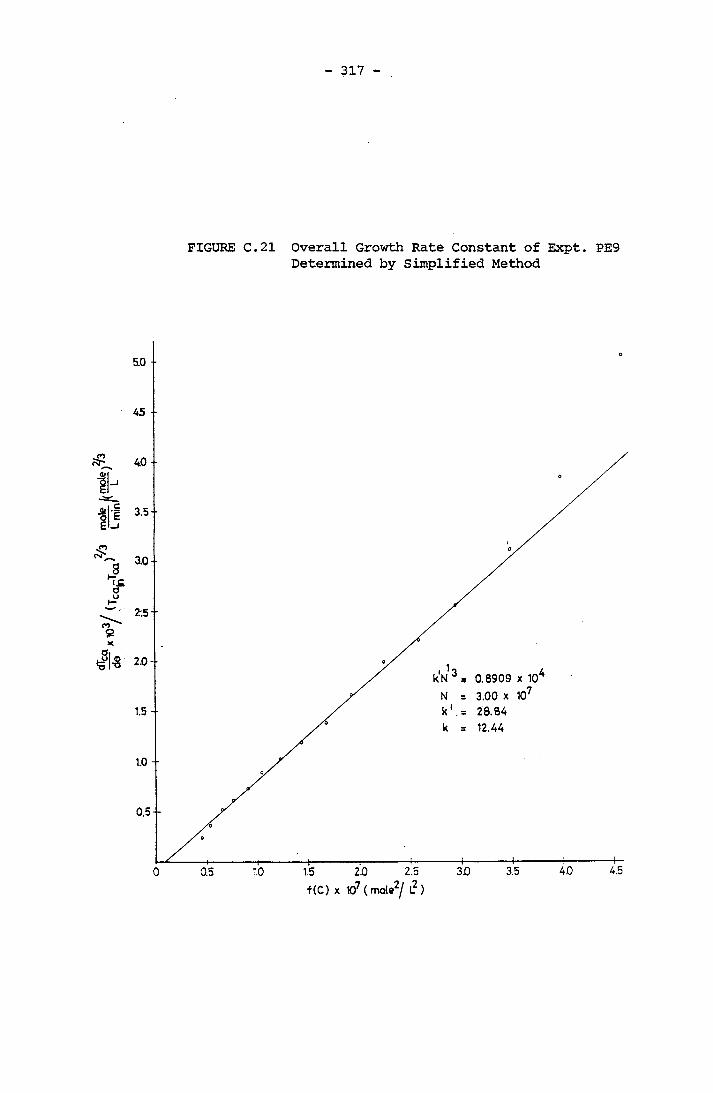
317
FIGURE C.21 Overall Growth Rate Constant of Expt. PE9 Determined by Simplified Method
0.8909 x 10' 3.00 x 10⁷ 28.84 12.44

318
FIGURE C.22 Overall Growth Rate Constant of Expt. PE9 Determined by Size Consideration
k = Q 6033
* (C) X 107 (mofe2/L2 )

FIGURE C .23 Desupersaturation Curve of Expt. PE11319
-8scssgo-o
2UJI
g
-i_----------------------1--------------------—
f-
O
QO CO
O
<T> <X>
sco00
CO
(1 /djoui) e0L*
200
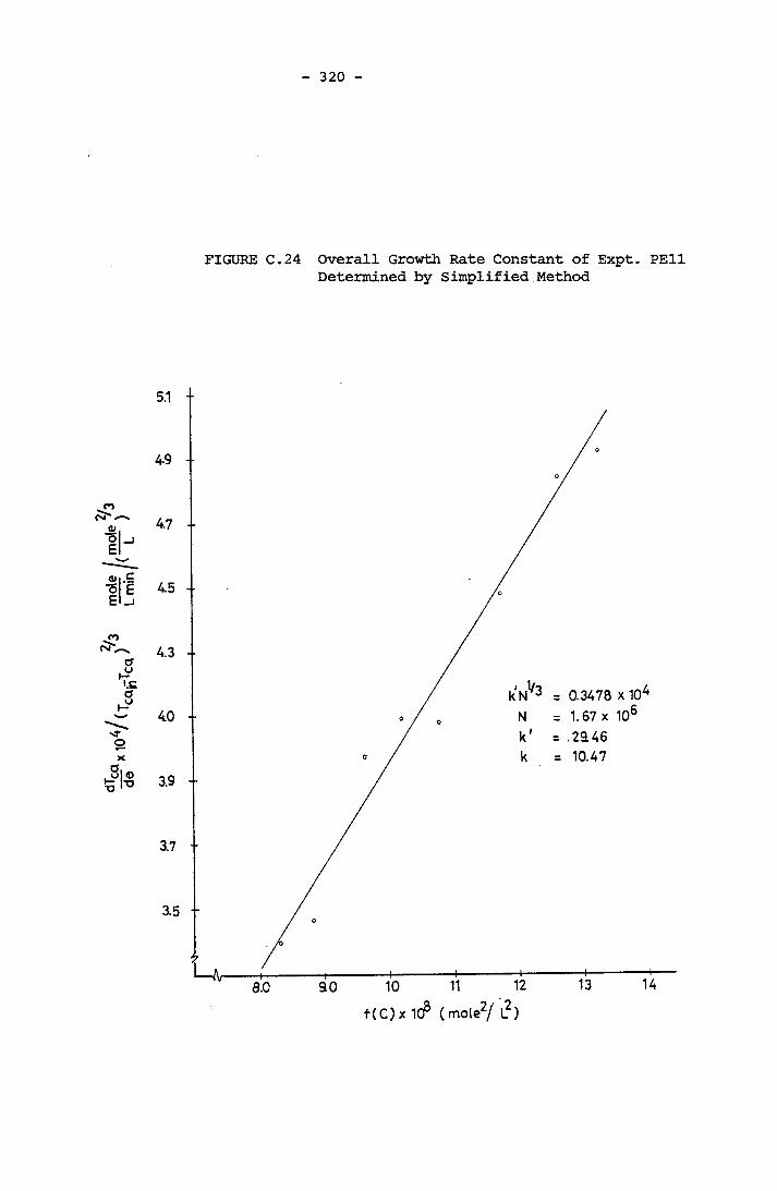
mol
e
320
FIGURE C.24 Overall Growth Rate Constant of Expt. PE11 Determined by Simplified Method
0.3478 x 10⁴
1.67 x 10⁶ 2£46 10.47
is -3

321
FIGURE C.25 Overall Growth Rate Constant of Expt. PE11 Determined by Size Consideration
------Ty------ 1--------------- 1--------------- 1--------------- t--------------- 1--------------- 1--------------- r-0.8 0.9 1.0 1.1 12 1.3 14
t(C) x 107 (mole2/l? )
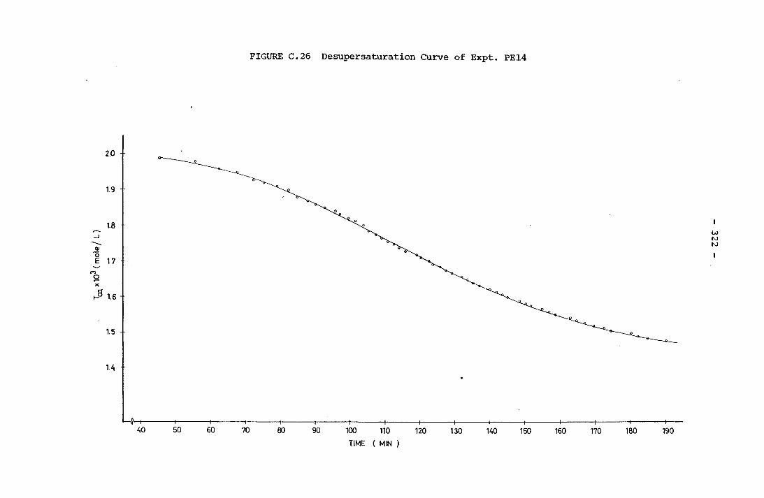
FIGURE C.26 Desupersaturation Curve of Expt. PE14322
(1 /aiouj)eoixmi
( MIN
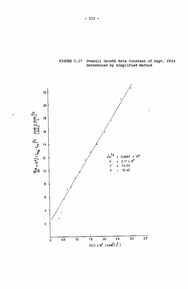
323
FIGURE C.27 Overall Growth Rate Constant of Expt. PE14 Determined by Simplified Method
0.6667 x 10'
24,0410.40
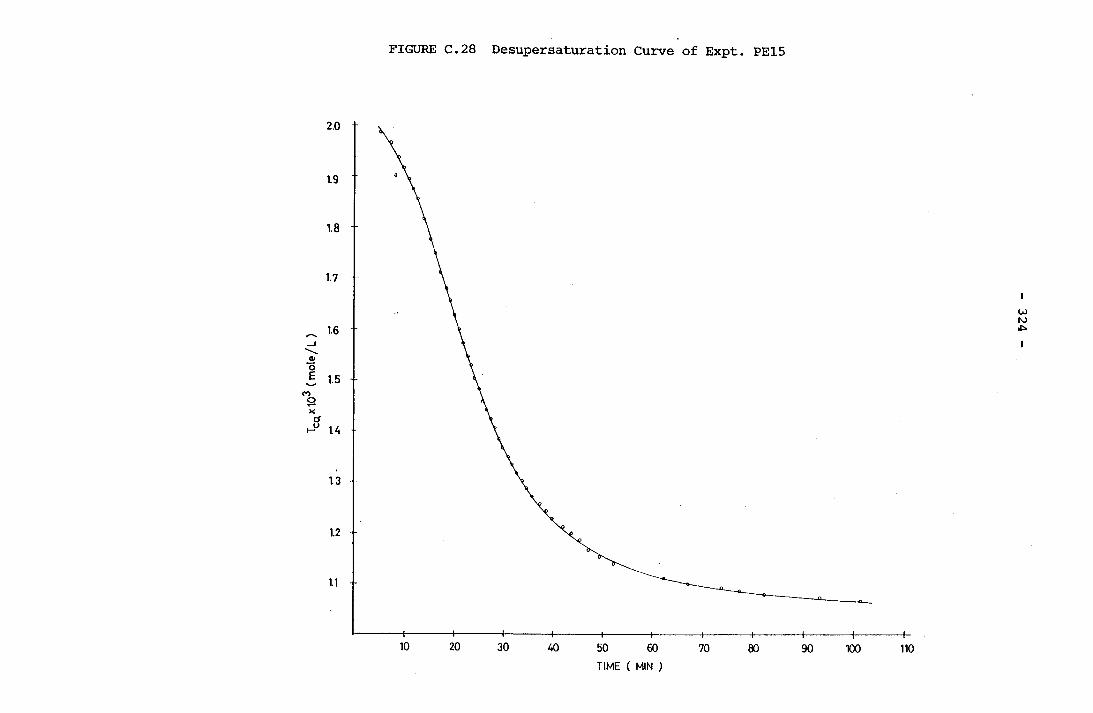
FIGURE C .28 Desupersaturation Curve of Expt. PE15324
'ME ( MIN

325
2.2721 x 10
2.60 x 10‘
35.8318.53
FIGURE C.29 Overall Growth Rate Constant of Expt. PE15 Determined by Simplified Method

- 326 -
FIGURE C.30 Overall Growth Rate Constant of Expt. PE15 Determined by Size Consideration
2.021
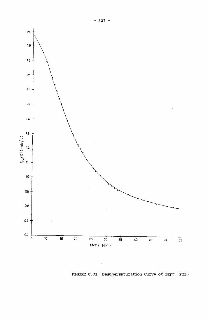
327
0.7 --
TIME ( MIN )
FIGURE C.31 Desupersaturation Curve of Expt. PE16

328
FIGURE C.32 Overall Growth Rate Constant of Expt. PE16 Determined by Simplified Method
2.3091 x 10⁴
8.50 x 10⁸
k = 12.70
f (C) x 107 (mole2/ l_2 )

FIGURE C.33 Desupersaturation Curve of Expt. PE21329
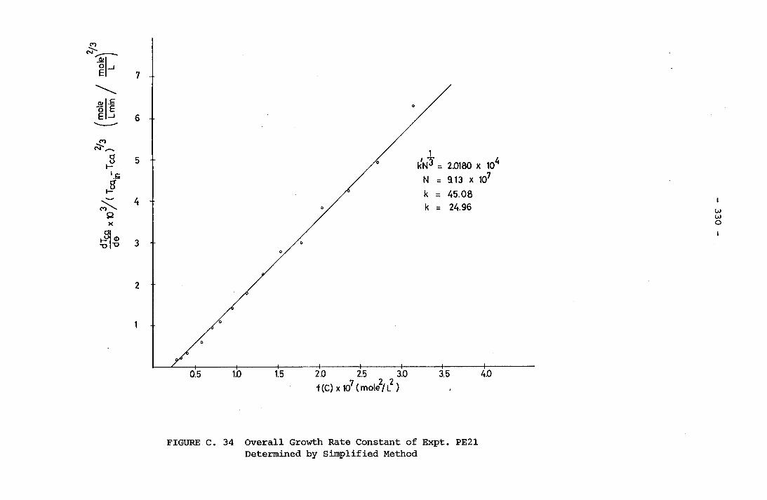
330
o cn
FIGURE C. 34 Overall Growth Rate Constant of Expt. PE21 Determined by Simplified Method

331
APPENDIX D RESULTS OF FINAL CRYSTAL SIZE MEASUREMENT
Some of the final crystal precipitates from the spontaneous crysta
llization experiments were sampled and sized by the Micro-videomat 2 Image Analyzer described in Section (4.4.3.3). This information is used
for crystal growth rate constant calculation using the Overall Growth
Rate with Size Consideration method described in Section (4.3.5). The data of crystal size measurement are presented in number distribution.
They are tabulated in the following tables:
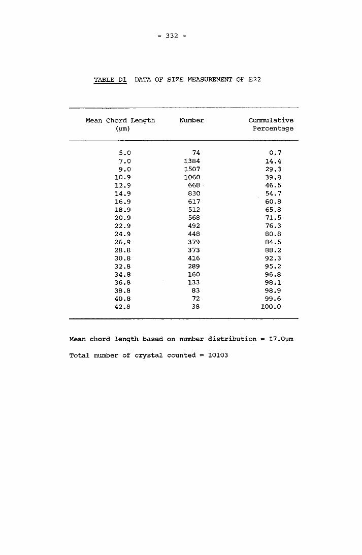
332
TABLE Dl DATA OF SIZE MEASUREMENT OF E22
Mean Chord Length (ym)
Number CummulativePercentage
5.0 74 0.77.0 1384 14.49.0 1507 29.3
10.9 1060 39.812.9 668 46.514.9 830 54.716.9 617 60.818.9 512 65.820.9 568 71.522.9 492 76.324.9 448 80.826.9 379 84.528.8 373 88.230.8 416 92.332.8 289 95.234.8 160 96.836.8 133 98.138.8 83 98.940.8 72 99.642.8 38 100.0
Mean chord length based on number distribution = 17.0ymTotal number of crystal counted = 10103
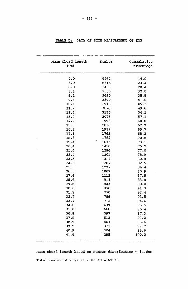
333
TABLE D2 DATA OF SIZE MEASUREMENT OF E23
Mean Chord Length (pm)
Number CummulativePercentage
4.0 9762 14.05.0 6516 23.46.0 3458 28.47.1 25.5 32.08.1 2680 35.89.1 3590 41.0
10.1 2916 45.211.2 3078 49.612.2 3130 54.113.2 2076 57.114.2 1995 60.015.3 2036 62.916.3 1937 65.717.3 1763 68.218.3 1752 70.819.4 1613 73.120.4 1450 75.221.4 1296 77.022.4 1301 78.923.5 1317 80.824.5 1207 82.525.5 1297 84.426.5 1067 85.927.6 1112 87.528.6 915 88.829.6 843 90.030.6 876 91.331.7 770 92.432.7 788 93.533.7 712 94.634.8 639 95.535.8 666 96.436.8 597 97.337.8 512 98.038.9 403 98.639.9 371 99.240.9 304 99.641.9 285 100.0
Mean chord length based on number distribution = 14.6pm
Total number of crystal counted = 69535

334
TABLE D3 DATA OF SIZE MEASUREMENT OF E24
Mean Chord Length Number(ym)
CummulativePercentage
3.2 557 5.83.6 389 9.94.1 518 15.34.5 377 19.35.0 395 23.45.5 325 26.85.9 301 30.06.4 434 34.56.8 283 37.57.3 354 41.27.7 375 45.18.2 364 48.98.6 395 53.19.1 267 55.99.6 242 58.4
10.0 259 61.110.5 144 62.610.9 137 64.111.4 162 65.811.8 155 67.412.3 130 68.812.7 118 70.013.2 85 70.913.6 105 72.014.1 113 73.214.6 83 74.015.0 130 75.415.5 86 76.315.9 97 77.316.4 82 78.216.8 57 78.817.3 79 79.617.7 81 80.418.2 71 81.218.7 23 81.419.1 56 82.019.6 100 83.120.0 39 83.520.5 118 84.720.9 40 85.121.4 86 86.021.8 73 86.822.3 62 87.422.7 56 88.023.2 96 89.023.7 74 89.824.1 62 90.524.6 85 91.3
(cont'd)
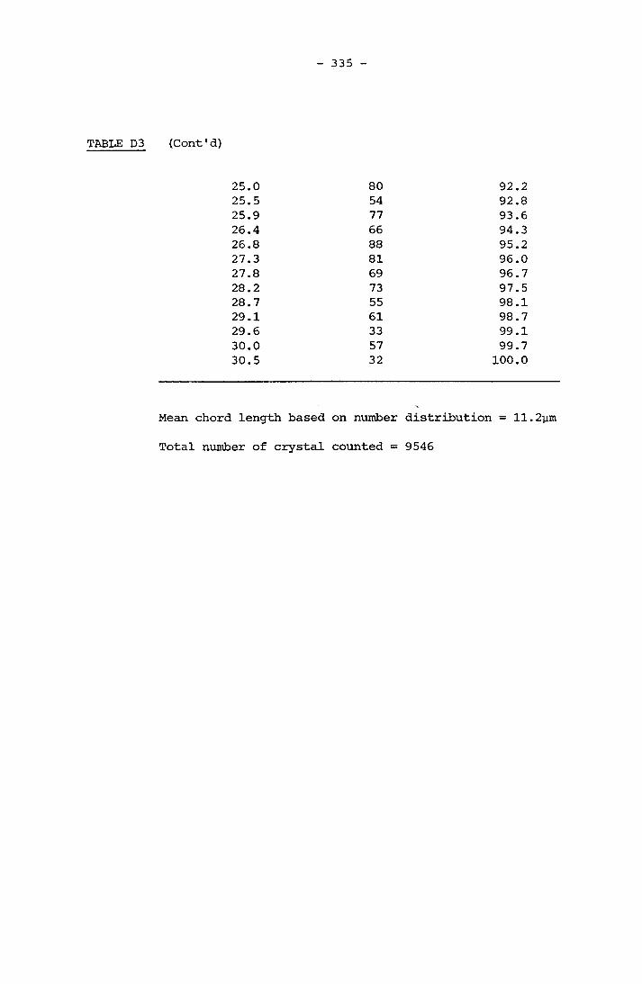
335
TABLE D3 (Cont'd)
25.0 80 92.225.5 54 92.825.9 77 93.626.4 66 94.326.8 88 95.227.3 81 96.027.8 69 96.728.2 73 97.528.7 55 98.129.1 61 98.729.6 33 99.130.0 57 99.730.5 32 100.0
1 length based on number distribution = 11Total number of crystal counted = 9546

336
TABLE D4 DATA OF SIZE MEASUREMENT OF PE4
Mean chord length (ym)
Number CummulativePercentage
0.5 3303 15.91.4 4148 35.82.4 2831 49.43.3 1895 58.54.3 1642 66.45.2 1330 72.76.1 1314 79.17.1 1116 84.48.0 823 88.49.0 743 91.99.9 496 94.3
10.9 384 96.211.8 184 97.012.8 233 98.213.7 77 98.514.7 75 98.915.6 88 99.316.5 42 99.517.5 26 99.618.4 27 99.819.4 35 99.920.3 14 100.0
Mean chord length based on number distribution = 4.0ymTotal number of crystal counted = 20826
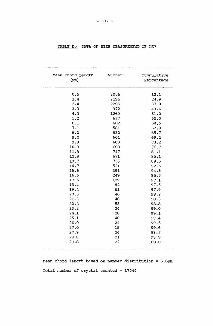
337
TABLE D5 DATA OF SIZE MEASUREMENT OF PE7
Mean Chord Length (ym)
Number CummulativePercentage
0.5 2056 12.11.4 2196 24.92.4 2206 37.93.3 972 43.64.3 1269 51.05.2 677 55.06.1 602 58.57.1 581 62.08..0 632 65.79.0 601 69.29.9 688 73.2
10.9 600 76.711.8 747 81.112.8 671 85.113.7 755 89.514.7 521 92.515.6 391 94.816.6 249 96.317.5 129 97.118.4 82 97.519.4 61 97.920.3 46 98.221.3 48 98.522.2 53 98.823.2 34 99.024.1 28 99.125.1 40 99.426.0 24 99.527.0 18 99.627.9 24 99.728.8 21 99.929.8 22 100.0
Mean chord length based on number distribution = 6.6ym
Total number of crystal counted = 17044
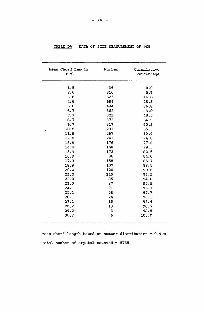
338
TABLE D6 DATA OF SIZE MEASUREMENT OF PE8
Mean Chord Length (ym)
Number CummulativePercentage
1.5 36 0.62.6 310 5.93.6 623 16.64.6 684 28.35.6 494 36.86.7 362 43.07.7 321 48.58.7 372 54.99.7 317 60.310.8 291 65.311.8 267 69.912.8 241 74.013.8 176 77.014.8 148 79.515.9 172 82.516.9 86 84.017.9 158 86.718.9 107 88.520.0 120 90.621.0 115 92.522.0 85 94.023.0 87 95.524.1 71 96.725.1 58 97.726.1 24 98.127.1 15 98.428.2 19 98.729.2 3 98.830.2 6 100.0
Mean chord length based on number distribution = 9.9ym Total number of crystal counted = 5768
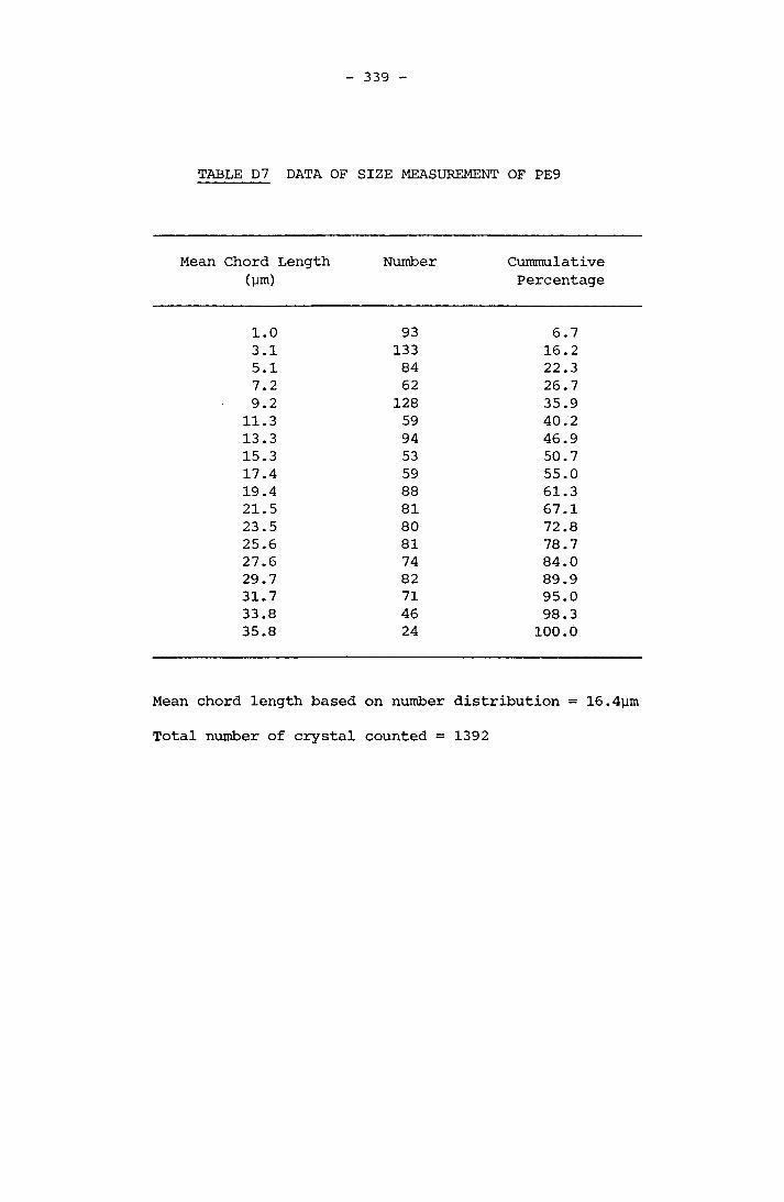
TABLE D7 DATA OF SIZE MEASUREMENT OF PE9
Mean Chord Length (ym)
Number CummulativePercentage
1.0 93 6.73.1 133 16.25.1 84 22.37.2 62 26.79.2 128 35.9
11.3 59 40.213.3 94 46.915.3 53 50.717.4 59 55.019.4 88 61.321.5 81 67.123.5 80 72.825.6 81 78.727.6 74 84.029.7 82 89.931.7 71 95.033.8 46 98.335.8 24 100.0
Mean chord length based on number distribution = 16.4ym
Total number of crystal counted = 1392

TABLE D8 DATA OF SIZE MEASUREMENT OF PE11
Mean Chord Length (yin)
Number CummulativePercentage
20.8 3 0.622.5 8 2.324.3 5 3.326.0 21 7.627.7 1 7.829.4 21 12.231.1 0 12.232.8 16 15.534.5 1 15.736.2 10 17.738.0 15 20.839.7 0 20.841.4 26 26.243.1 9 28.044.8 21 32.446.5 18 36.148.2 17 39.649.9 25 44.751.6 32 51.353.4 54 62.555.1 76 78.156.8 106 100.0
Mean chord length based on number distribution = 47.6ym
Total number of crystal counted = 485
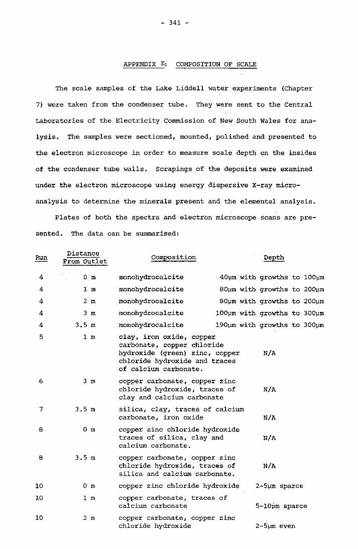
341
APPENDIX E: COMPOSITION OF SCALE
The scale samples of the Lake Liddell water experiments (Chapter
7) were taken from the condenser tube. They were sent to the Central Laboratories of the Electricity Commission of New South Wales for analysis. The samples were sectioned, mounted, polished and presented to
the electron microscope in order to measure scale depth on the insides of the condenser tube walls. Scrapings of the deposits were examined
under the electron microscope using energy dispersive X-ray micro
analysis to determine the minerals present and the elemental analysis.Plates of both the spectra and electron microscope scans are pre
sented. The data can be summarised:
Run
444445
6
7
8
8
1010
Distance From Outlet
0 m1 m2 m3 m
3.5m1 m
3 m
3.5 m
0 m
3.5m
0 m1 m
2 m
Composition Depth
monohydrocalcite 40ym with growths to lOOymmonohydrocalcitemonohydrocalcitemonohydrocalcite
80ym with growths to 200ym 80ym with growths to 200ym lOOym with growths to 300ym
monohydrocalcite 190ym with growths to 300ymclay, iron oxide, coppercarbonate, copper chloridehydroxide (green) zinc, copper N/Achloride hydroxide and tracesof calcium carbonate.copper carbonate, copper zinc chloride hydroxide, traces of N/Aclay and calcium carbonatesilica, clay, traces of calcium carbonate, iron oxide N/Acopper zinc chloride hydroxidetraces of silica, clay and N/Acalcium carbonate.copper carbonate, copper zinc chloride hydroxide, traces of N/Asilica and calcium carbonate.copper zinc chloride hydroxidecopper carbonate, traces of calcium carbonatecopper carbonate, copper zinc chloride hydroxide
2-5ym sparce
5-10ym sparce
2-5ym even10
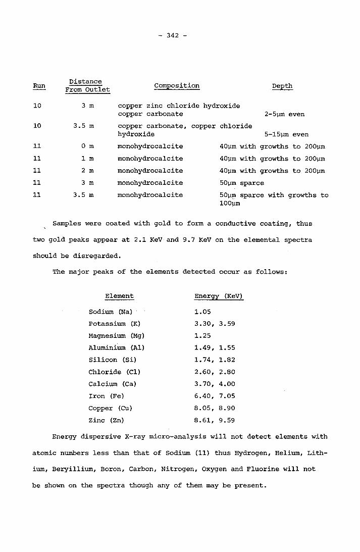
342
Run DistanceFrom Outlet Composition Depth
10 3 m copper zinc chloride hydroxide copper carbonate 2-5ym even
10 3.5 m copper carbonate, copper hydroxide
chloride5-15ym even
11 0 m monohydrocalcite 40ym with growths to 200ym11 1 m monohydrocalcite 40ym with growths to 200ym11 2 m monohydrocalcite 40ym with growths to 200ym11 3 m monohydrocalcite 50ym sparce11 3.5m monohydrocalcite 50ym sparce with growths to
lOOym
Samples were coated with gold to form a conductive coating, thus
two gold peaks appear at 2.1 KeV and 9.7 KeV on the elemental spectra should be disregarded.
The major peaks of the elements detected occur as follows:
Element Energy (KeV)Sodium (Na) 1.05Potassium (K) 3.30, 3.59Magnesium (Mg) 1.25Aluminium (Al) 1.49, 1.55Silicon (Si) 1.74, 1.82Chloride (Cl) 2.60, 2.80Calcium (Ca) 3.70, 4.00Iron (Fe) 6.40, 7.05Copper (Cu) 8.05, 8.90Zinc (Zn) 8.61, 9.59
Energy dispersive X-ray micro-analysis will not detect elements with
atomic numbers less than that of Sodium (11) thus Hydrogen, Helium, Lithium, Beryillium, Boron, Carbon, Nitrogen, Oxygen and Fluorine will not
be shown on the spectra though any of them may be present.

343
PLATE El Run 4, 0 m scale, lOOOx magnification, H.F.W. 0.2 5mm.
PLATE E2 Run 4, 1 m scale, 2100x magfication, H.F.W. 0.05mm

344
PLATE E3 Run 4, 1 m scale, 5259x magnification, H.F.W. 0.02mm
PLATE E4 Run 4, 2m scale, 1500x magnification, H.F.W. 0.83mm.

345
PLATE E5 Run 4, 3m scale, 1700x magnification, H.F.W. 0.73mm.
PLATE E6 Run 4, 3.5 m scale, 1300x magnification, H.F.W. 0.96mm.

346
PLATE E7 Spectra run 4, 0 m, monohydrocalcite.
PLATE E8 Spectra run 4, l.o m, monohydrocalcite.

-347
PLATE E9 Spectra run 4, 2.0 m, monohydrocalcite and traces of iron.
PLATE E10 Spectra run 4, 3.5 m, monohydrocalcite and traces of copper.
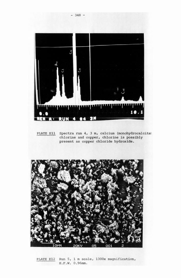
348
PLATE Ell Spectra run 4, 3 m, calcium (monohydrocalcite chlorine and copper, chlorine is possibly present as copper chloride hydroxide.
PLATE El2 Run 5, 1 m scale, 1300x magnification, H.F.W. 0.96mm.

349
PLATE El3 Spectra run 5, 1 m
PLATE E14 Run 6, 3m scale, 650x magnification, H.F.W. 0.92mm.

350
PLATE El5 Spectra run 6, 3m.
PLATE E16 Run 7, 3.5m scale, 650x magnification,H.F.W. 0.67mm, note angular grain of silica in top right.

351
PLATE E18 Run 8, Om scale, 800x magnification, H.F.W. 0.156mm.
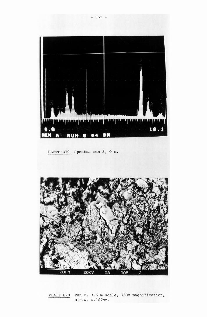
352
PLATE E19 Spectra run 8, 0 m.
PLATE E20 Run 8, 3.5 m scale, 750x magnification, H.F.W. 0.167mm.
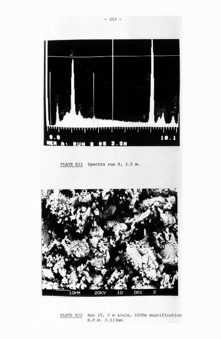
353
PLATE E21 Spectra run 8, 3.5 m.
PLATE E22 Run 10, 0 m scale, HOOx magnification H.F.W. 0.113mm.
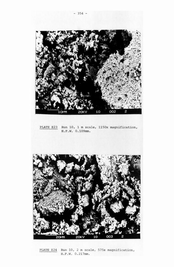
354
PLATE E23 Run 10, 1 m scale, 1150x magnification, H.F.W. 0.109mm.
PLATE E24 Run 10, 2m scale, 575x magnification, H.F.W. 0.217mm.

355
PLATE E25 Run 10, 3m scale, HOOx magnification, H.F.W. 0.114mm.
PLATE E26 Run 10, 3.5 m scale, 575x magnification, H.F.W. 0.217mm.

PLATE E27 Spectra run 10, 0 m.
PLATE E28 Spectra run 10, 1 m.

357
PLATE E29 Spectra run 10, 2m.
PLATE E30 Spectra run 10, 3m.

358
PLATE E32 Run 11, 1 m scale, 1250x magnification, H.F.W. 0.1mm.
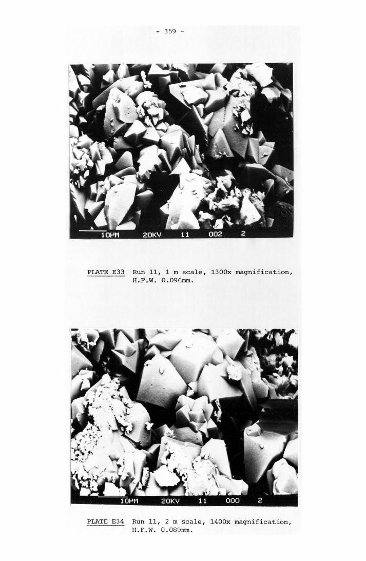
359
PLATE E33 Run 11, 1 m scale, 1300x magnification, H.F.W. 0.096mm.
PLATE E34 Run 11, 2m scale, 1400x magnification, H.F.W. 0.089mm.
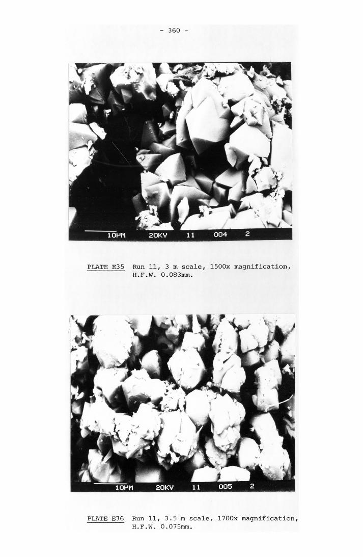
360
PLATE E35 Run 11, 3m scale, 1500x magnification, H.F.W. 0.083mm.
PLATE E36 Run 11, 3.5 m scale, 1700x magnification, H.F.W. 0.075mm.

361
PLATE E38 Spectra run 11, 1 m.
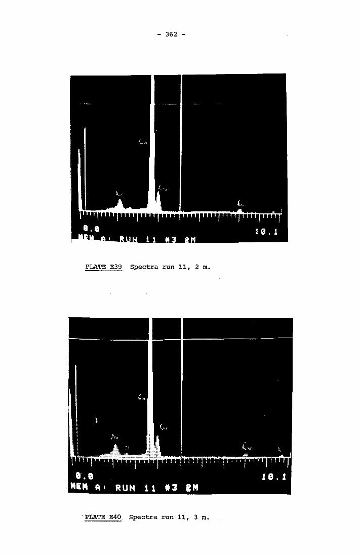
362
PLATE E40 Spectra run 11, 3m.
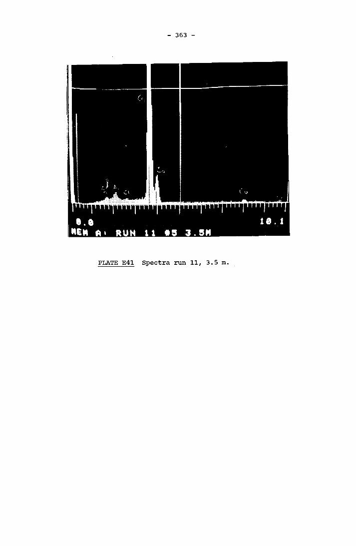
363
PLATE E41 Spectra run 11, 3.5m.

364
APPENDIX F LISTINGS OF PROGRAMMES
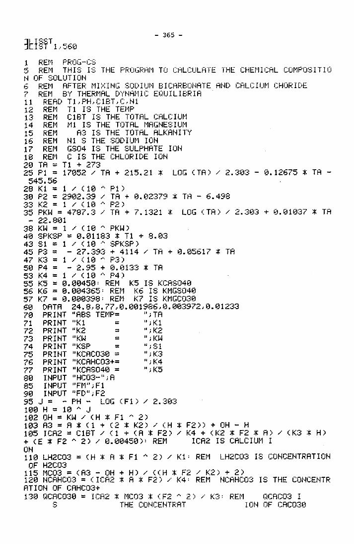
3653b1§¥T1,560I REM PROG-CS5 REM THIS IS THE PROGERM TO CALCULATE THE CHEMICAL COMPOSIT ID N OF SOLUTION6 REM AFTER MIXING SODIUM BICARBONATE AND CALCIUM CHOPIDE7 REM BY THERMAL DYNAMIC EQUILIBRIAII READ T1,PH,C1BT,C,N112 REM T1 IS THE TEMP13 REM C1BT IS THE TOTAL CALCIUM14 REM Ml IS THE TOTAL MAGNESIUM15 REM A3 IS THE TOTAL ALKANITY16 REM N1 S THE SODIUM ION17 REM GS04 IS THE SULPHATE ION18 REM C IS THE CHLORIDE ION 20 TA = T1 + 27325 PI = 17852 / TA + 215.21 % LOG (TA > / 2.303 - 0.12675 * TA - 545.56
28 K1 = 1/(10 PI)30 P2 = 2902.39 / TA + 0.02379 * TA - 6.498 33 K2 = 1 / (10 P2>35 PKUI = 4787.3 / TA + 7.1321 X LOG (TA > / 2.303 + 8.01037 X TA - 22.801
38 KM = 1 / (18 * PKUI)40 SPKSP = 0.01183 X T1 + 8.03 43 SI = 1 / (10 * SPKSP)45 P3 = - 27.393 + 4114 / TA + 0.05617 X TA47 K3 = 1 / (10 P3)50 P4 = - 2.95 + 8.0133 X TA53 K4 = 1 / (18 P4)55 K5 = 0.00450= REM K5 IS KCASQ4056 K6 = 0.004365: REM K6 IS KMGSO4057 K7 = 0.000398- REM K7 IS KMGCO3060 DATA 24.8,8.77,0.001986,0. 003972,8.0123370 PRINT "ABS TEMP= "; TA71 PRINT "K1 " j K172 PRINT "K2 "; K273 PRINT "KW "; KN74 PRINT "KSP "S175 PRINT "KCACO30 = "; K376 PRINT "KCAHC03+= "; K477 PRINT "KCASO40 = "; K580 INPUT " HC03- " A85 INPUT "FM";F190 INPUT "FD";F295 J = - PH - LOG (FI) / 2.303100 H = 10 J102 OH = KN / (H X FI 2)103 A3 = A X (1 + (2 X K2) / (H X F2 )) + OH - H105 ICA2 = C1BT / (1 + (A X F2 ) / K4 + (K2 X F2 X A) / (K3 X H)+ (E ON
X F2 * 2) / 0.00450) = REM ICA2 IS CALCIUM I110 LH2C03 = (H X A X FI ^ 2) / K1 : REM LH2C03 IS CONCENTRATIONOF H2C03115 MC03 = (A3 - OH + H) / ((H *: F2 / K2) + 2)120 NCAHC03 = (ICA2 X A X F2) / K4: REM NCAHC03 IS THE CONCENTRATION OF CAHC03+130 QCACO30 = ICA2 X MC03 X (F2 ^ 2) / K3; REM QCAC03 I
S THE CONCENTEAT ION OF CACO30

366
139 3 = 0.5 X (Ml + H + 4 X ICRS + NCRHCQ3 + C + OH + R + 4 03 >140 U = < SQR <S> / (1 + SQR < S > > > - 0.3 % S145 FI = 10 's < - 0.5 X IJ>150 F2 = 10 < - 2.0 * U>157 C2 = LH2C03 + R + MC03 + QCRC03 + NCRHC03370 fll = HI + 2 % ICR2 + H + NCRHC03 - C - OH - 2 % MC03375 IF fll > <fl) THEN GOTO 400380 IF RB3 <fl - fll> < <0.001 X fl> THEN GOTO 500 335 fl = fl - 0.01 % R 390 PRINT "fl TOO BIG";A 395 GOTO 95400 IF <0.99 X fll> < <R> THEN GOTO 450405 fl * R + 0.01 X R410 PRINT "fl TOO SMALL";fl415 GOTO 95450 R = A + 0.0001 X R455 PRINT "fl LITTLE TOO SMALL" ;R460500510515520525530535540550552554560
GOTO 95S3 = ICR2 * MC03 X <F2 * 2> / SI PRINT "TOTAL CRRB0N=";C2 PRINT "HC03=";R PRINT "C03= "MC03 PRINT "H2C03=";LH2C03 PRINT "CRCO30=“;QCRC03 PRINT "CflHC03+=";NCRHC03 PRINT "CA+="iICR2PRINT "DEGREE OF SUPERSflTURRTION®";S3 PRINT "FM=" F1 PRINT "FD="F2 STOP
X MC
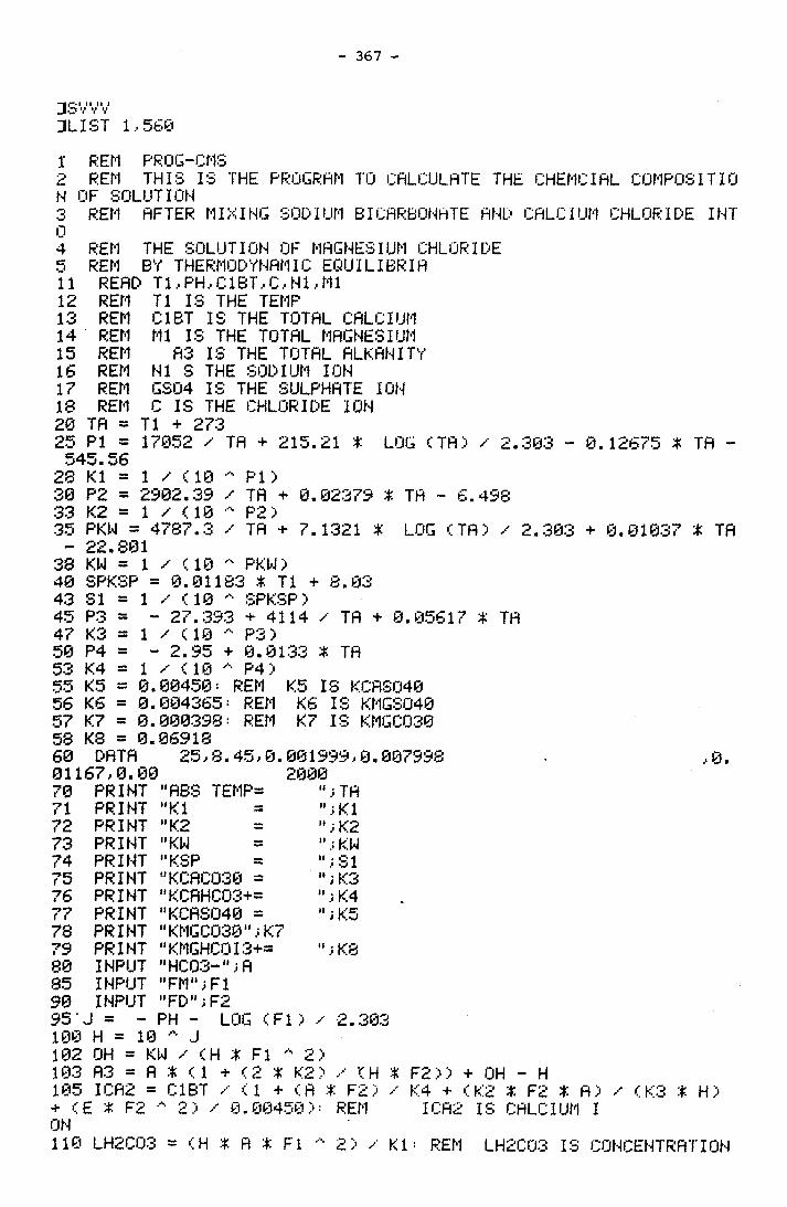
367
“1 <*"• I II II lJo V V V
JLIST 1,560 r REM PR06-CMS2 REM THIS IS THE PROGRAM TO CALCULATE THE CHEMCIAL COMPOSIT IQ N OF SOLUTION3 REM AFTER MIXING SODIUM BICARBONATE AND CALCIUM CHLORIDE INT04 REM THE SOLUTION OF MAGNESIUM CHLORIDE5 REM BY THERMODYNAMIC EQUILIBRIA11 READ T1,PH,C1BT,C,N1,M112 REM T1 IS THE TEMP13 REM C1BT IS THE TOTAL CALCIUM14 REM Ml IS THE TOTAL MAGNESIUM15 REM A3 IS THE TOTAL ALLANITY16 REM N1 S THE SODIUM ION17 REM GS04 IS THE SULPHATE ION18 REM C IS THE CHLORIDE ION 20 TA = T1 + 27325 PI = 17052 / TA + 215.21 * LOG (TA) ✓ 2.303 - 0.12675 * TA - 545.5628 K1 = 1 / (10 PI)30 P2 = 2902.39 / TA + 0.02379 * TA - 6.498 33 K2 = 1 / (10 P2>35 PKW = 4787.3 ✓ TA + 7.1321 * LOG (TA) ✓ 2.303 + 0.01037 * TA __ 22.80138 KW* = 1 / (10 PKW)40 SPKSP = 0.01183 * T1 + 8.03 43 SI = 1 ✓ (10 's SPKSP)45 P3 = 27.393 + 4114 ✓ TA + 0.05617 4 TA47 K3 = 1 / (10 P3)50 P4 = - 2.95 + 0.0133 X TA53 K4 = 1 / (10 P4)55 K5 = 0.00450: REM K5 IS KCASO4056 K6 = 0.004365= REM K6 IS KMGSO4057 K7 = 0.000398= REM K7 IS KMGCQ3058 K8 = 0.0691860 DATA 25,8.45,0.001999,0.007998 ,0.01167,0.00 200070 PRINT "ABS TEMP* "TA71 PRINT "K1 " ;K172 PRINT "K2 " f K273 PRINT "KW "; KW74 PRINT "KSP "jSI75 PRINT "KCACO30 a "; K376 PRINT "KCAHC03+= "K477 PRINT "KCASO40 = "; K578 PRINT "KMGCO30";K779 PRINT "KMGHC0I3+a "K880 INPUT "HC03“";A85 INPUT "FM";FI90 INPUT "FD";F295 J = - PH - LOG (FI) / 2.303100 H = 10 ^ J102 OH a KW ✓ (H X FI " 2)103 A3 a A X (1 + (2 X K2) / (H X F2)) + OH - H105 ICA2 = C1BT (1 + (A X F2) / K4 + (K2 X F2 X A) / (K3 X H)+ (E X F2 A 2) / 0.00450)= REM ICA2 IS CALCIUM I ON110 LH2C03 = (H X A X FI A 2) / K1= REM LH2C03 IS CONCENTRATION
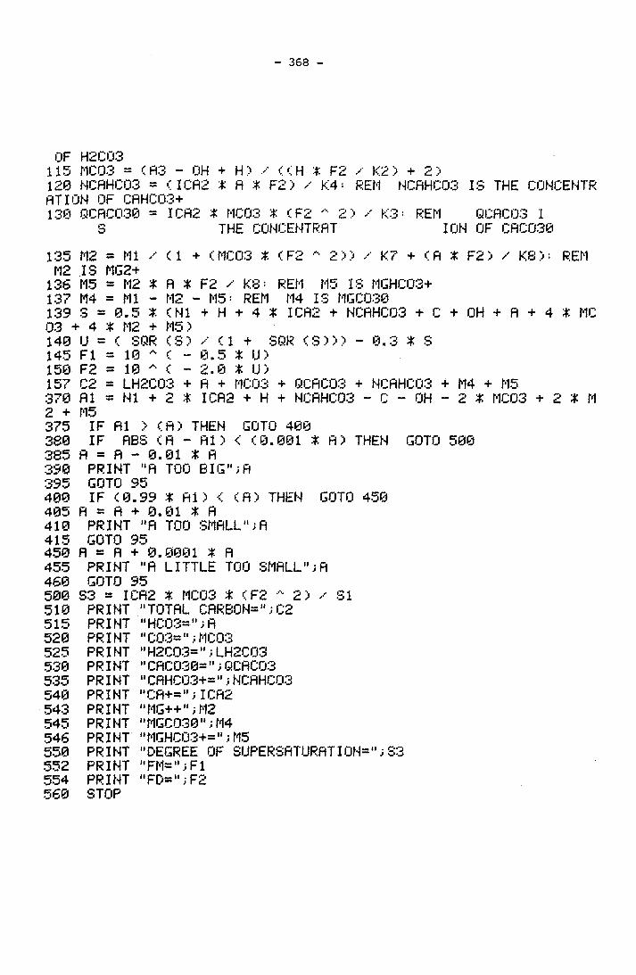
368
OF H2C03t15 MC03 = (AS - OH + H) / ((H * F2 ✓ K2 > + 2)120 NCftHCOS = CICR2 * ft * F2> / K4= REM NCAHC03 IS THE CONCENTR ftTIUN OF CHHC03+130 QCRCO30 = I Cft2 * MC03 4: (F2 * 2) ✓ K3 • REM QCftCOS I
S THE CONCENTRE!T ION OF CACO30135 M2 = Ml ✓ (1 + < MC03 t ( F2 "• 2>> / K7 + < ft * F2> / K8) = REM M2 IS MG2+136 M5 = M2 * ft * F2 / K8= REM M5 IS MGHC03+137 M4 * Ml - M2 - M5: REM M4 IS MGCO30139 S = 0.5 * <N1 + H + 4 * ICA2 + NCAHC03 +C+0H+fi+4*MC 03 + 4 * M2 + M5>140 U = ( SQR (S) y (.1 + SQR (S>)> - 0.3 * S145 FI = 10 ( - 0.5 * U>150 F2 = 10 ~ < - 2.0 I U)157 C2 = LH2C03 + ft + MC03 + QCftCOS + NCftHCOS + M4 + MS370 Ell = N1 +2 X ICA2 + H + NCftHCOS - C - OH - 2 X MC03 + 2 X M2 + M5375 IF Ell > (ft) THEN GOTO 480380 IF ABS (ft - Ell) < (0.001 X ft) THEN GOTO 500 385 ft a ft - 0.01 X ft 390 PRINT "ft TOO BIG";ft 395 GOTO 95400 IF (0.99 * Ell) < (ft) THEN GOTO 450405 ft = ft + 0.01 * ft410 PRINT "ft TOO SMALL";ft415 GOTO 95450 ft = ft + 0.0001 X ft455 PRINT "ft LITTLE TOO SMALL";ft460 GOTO :95500 S3 = ICEI2 * MC03 X (F2 A 2) ✓ SI510 PRINT "TOTAL CfiRB0N=";C2515 PRINT "HC03=" ; ft520 PRINT "C03=";MC03525 PRINT "H2C03=";LH2C03530 PRINT MCftC030=";QCftCOS535 PRINT ,,CftHC03+="; NCftHCOS540 PRINT "CEl+=";ICA2543 PRINT "MG++";M2545 PRINT "MGCO30";M4546 PRINT "MGHC03+=";M5550 PRINT "DEGREE OF SUPERSfiTURftTIOW552 PRINT "FM=";FI554 PRINT "FD=";F2560 STOP
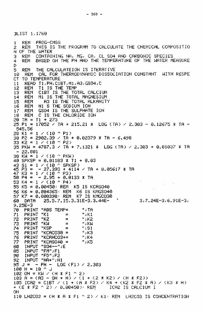
369
3LI3T 1,17601 REM PROG“CMS32 REM THIS IS THE PROGRAM TO CALCULATE THE CHEMICAL COMPOSIT10 N OF THE WATER3 REM CONTAINING NA, MG, CA, CL S04 AND CARBONIC SPECIES4 REM BASED ON THE PH AND THE TEMPERATURE OF THE WATER MEASURED5 REM THE CALCULATEION IS ITERATIVE10 REM CAL FOR THERMODYNAMIC DISSOCIATION CONSTANT WITH RESPE CT TO TEMPERATURE11 READ T1,PH,C1BT,M1,A3,GS04,C12 REM T1 IS THE TEMP13 REM C1BT IS THE TOTAL CALCIUM14 REM Ml IS THE TOTAL MAGNESIUM15 REM A3 IS THE TOTAL ALKANITY16 REM N1 S THE SODIUM ION17 REM GS04 IS THE SULPHATE ION IS REM C IS THE CHLORIDE ION20 TA = T1 + 27325 PI = 17052 / TA + 215.21 * LOG (TA) / 2.303 - 0.12675 * TA - 545.56
28 K1 = 1 / ( 10 PI >30 P2 * 2302.39 / TA + 0.02379 * TA - 6.498 33 K2 = 1 / (10 * P2>35 PKW = 4787.3 / TA + 7.1321 * LOG CTA) / 2.303 + 0.01037 * TA - 22.80138 KW =1/(10 PKW)
40 SPKSP = 0.01183 * T1 + 8.0343 SI = 1/(10 SPKSP)45 P3 = - 27.393 + 4114 / TA + 0.05617 X TA47 K3 = 1 / (10 * P3)50 P4 = - 2.95 + 0.0133 X TA53 K4 = 1 / <10 A P4)55 K5 = 0.00450: REM K5 IS KCASO40 P.6 K6 = 0.004365: REM K6 IS KMGSO40 57 K7 = 0.000398- REM K7 IS KMGCO3060 DATA 25.5,7.15,3.31E-3,3.44E- 7 3,7.24E-3,6.91E-3,9.25E-370 PRINT "ABS TEMP® "; TA71 PRINT MK1 " j K172 PRINT "K2 " i K273 PRINT "KW “; KW74 PRINT "KSP “; SI75 PRINT "KCACO30 = "; K376 PRINT "KCAHC03+= “; K477 PRINT "KCASO40 = " * K580 INPUT "S04—";E85 INPUT "FM";F190 INPUT "FD">F292 INPUT "NA+";N195 J = - PH ~ LOG (Fl) / 2.100 H = 10 * J102 OH = KW / <H X FI 2)103 A = (A3 ~ OH + H) / (1 + (2 X 10⁵ ICA2 = C1BT / (1 + (A X F2) / + (E X F2 2) / 0.00450)= REMON
K2 ) / (H X F2 ) )K4 + (K2 X F2 X A) / (K3 X H) ICA2 IS CALCIUM I
110 LH2C03 = (H X A X Fl 2) / K1 •* REM LH2C03 IS CONCENTRATION
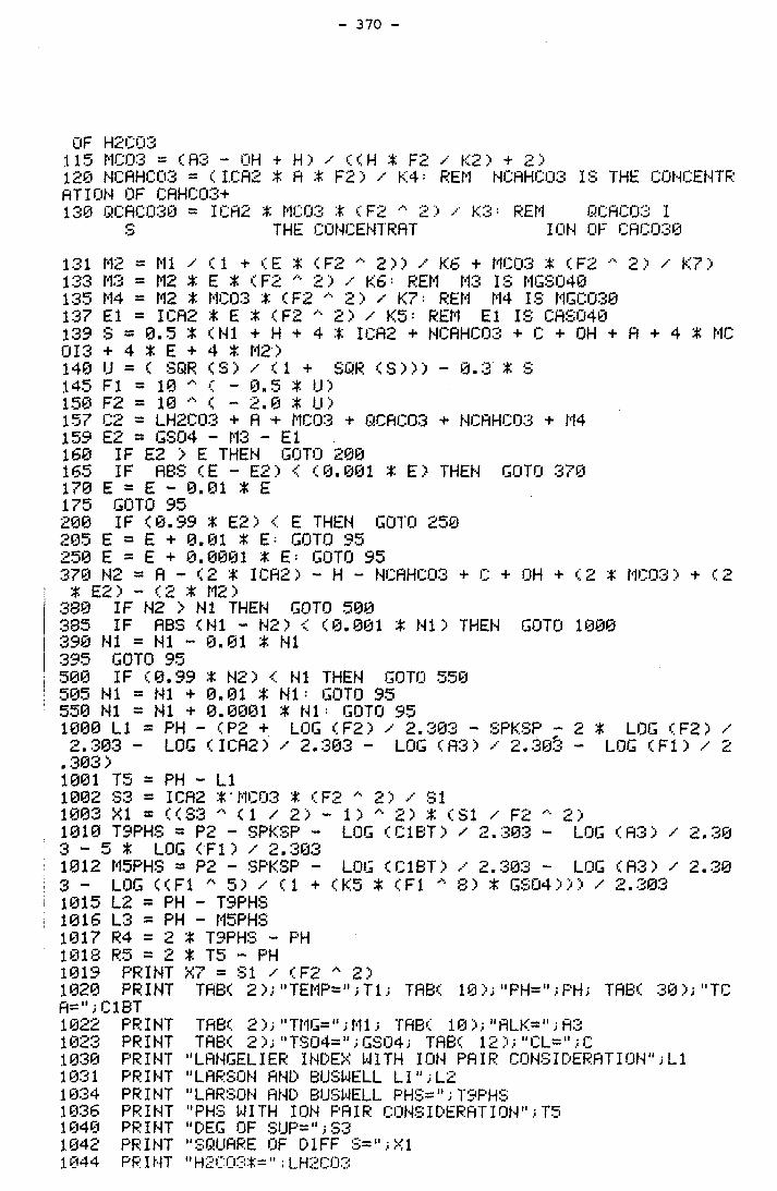
370
OF H2C03115 MC03 = (A3 - OH + H> / ((H % F2 / K2> + 2>120 NCRHC03 = CI.CA2 X R X F 2 > / K4 = REM NCRHC03 IS THE CONCENTR RTION OF CRHC03+130 QCRCO30 = ICR2 X MC03 X <F2 * 2> ✓ K3: REM QCRC03 I
S THE CONCENTRRT ION OF CRCO30131 M2 = Ml / (1 + (E * (F2 " 2)) / Kb + MC03 X ( F2 2) / K7) 133 M3 = M2 * E * ( F2 * 2) / Kb= REM M3 IS MGSO40135 M4 = M2 X MCQ3 X (F2 A 2> ✓ K? ■ REM M4 IS MGCO30137 El = ICR2 X E X <F2 * 2) / K5- REM El IS CRSO40139 S = 0.5 X (HI + H + 4 X ICR2 + NCRHC03 +C+0H+R+4* MCfl T 3 + 4 * F + 4 * M2 "j
140 U = ( SQR (S) / (1 + SQR ( S ) ) ) - 0.3 X S145 FI = 10 ~ < - 0.5 X U)150 F2 = 10 ( - 2.0 X U)157 C2 = LH2C03 + R + MC03 + QCRC03 + NCRHC03 + M4159 E2 = GS04 - M3 - El160 IF E2 > E THEN GOTO 200165 IF RBS (E - E2> < (0.001 X E> THEN GOTO 370 170 E = E ~ 0.01 X E 175 GOTO 95200 IF (0.99 X E2) < E THEN GOTO 258 205 E = E + 0.01 X E: GOTO 95 250 E = E + 8.0001 X E = GOTO 95370 N2 = R - (2 X ICR2) - H - NCRHC03 + C + OH + (2 X MC03) + (2 X E2 - < 2 X M2')
380 IF N2 > N1 THEN GOTO 500385 IF RBS (N1 - N2 ) < (0.001 X N1> THEN GOTO 1000 390 N1 = N1 - 0.01 X N1 3«nf=; 00TO 95580 IF (o'. 99 X N2) < N1 THEN GOTO 550 505 N1 « N1 + 0.01 X N1: GOTO 95 550 N1 = N1 + 0.0001 X Nl: GOTO 951000 LI = PH - (P2 + LOG (F2 > / 2.303 - SPKSP - 2 X LOG (F2) / 2.303 - LOG (ICR2) / 2.383 - LOG (R3> / 2.30$ - LOG (FI) / 2 . 303 )1001 T5 = PH - LI1002 S3 = ICR2 X'MC03 X (F2 * 2) / SI1803 XI * ((S3 * (1 / 2) ~ 1) * 2) X (SI / F2 * 2)1010 T9PHS = P2 - SPKSP - LOG (C1BT) / 2.303 - LOG (R3) / 2.30 3 ~ 5 X LOG (FI ) / 2.3031012 M5PHS = P2 - SPKSP - LOG (C1BT> / 2.303 - LOG (R3) / 2.303 - LOG ((FI 5) / (1 + (K5 X (FI A 8) X GS04))) / 2.3031015 L2 = PH - T9PHS1016 L3 = PH - M5PHS 1817 R4 = 2 X T9PHS - PH1018 R5 = 2 X T5 - PH1019 PRINT X7 = SI / (F2 * 2)1820 PRINT TRB( 2 );"TEMP=";T1; TRB( 10 ); "PH«" ;PH; TRB( 38);"TO fl=";C1BT1022 1823 1030 1831 1034 1036 1040 1042 1044
PRINT TRBC 2 );"TMG=";M1; TRB( 10);"RLK=";R3PRINT TREK 2 ); "TSG4="; GS04; TRBC 12 ); "CL=" ; CPRINT "LRNGELIER INDEX WITH ION PRIR CONSIDERATION";LIPRINT "LARSON AND BUSWELL LI";L2PRINT "LARSON AND BUSWELL PHS=";T9PHSPRINT "PH3 WITH ION PRIR CONSIDERATION";T5PRINT "DEG OF SUP=";S3PRINT "SQUARE OF D1FF S=";X1PR I NT " H2C03*= " LH2C03
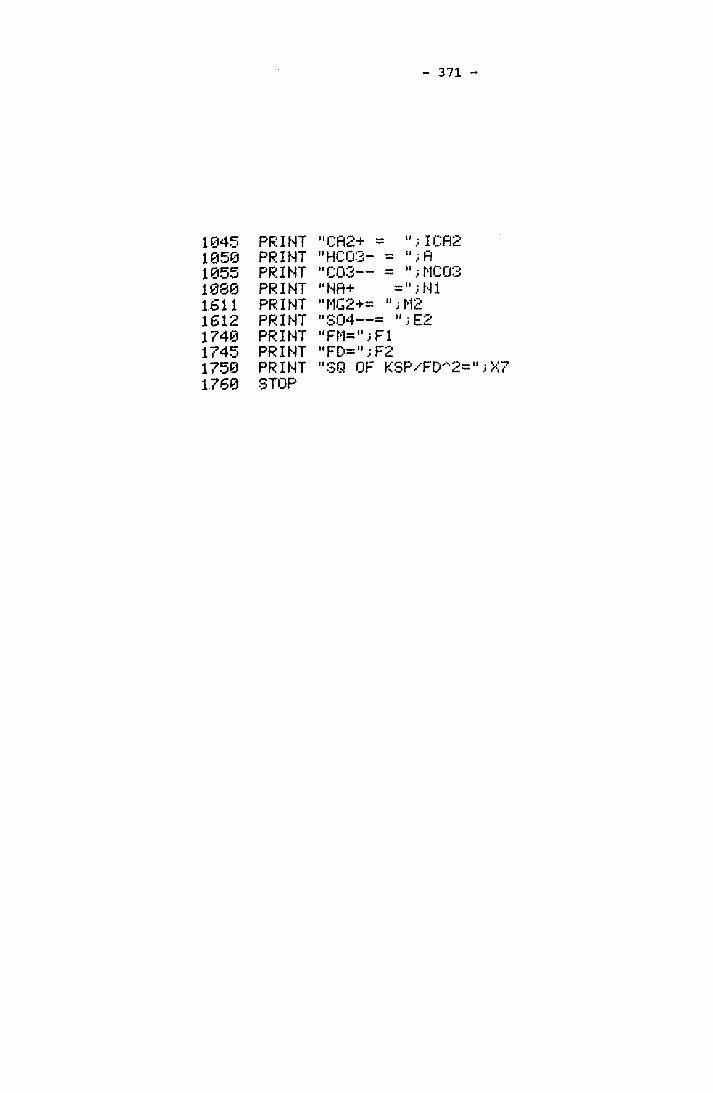
371
1045 PRINT "CR2+ = " ICR21050 PRINT "HC03- = " R1055 PRINT "C03— = ";MC031080 PRINT "NR+ ="•N11611 PRINT "MG2+= "M21612 PRINT "804—= " E21740 PRINT "FM=".;F11745 PRINT "FD=";F217501760
PRINTSTOP
"SQ OF KSP/FD'“2
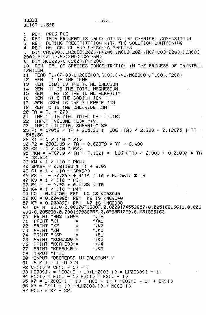
j:m:iJL1ST 1,590
372
1 REM PROG-PCS2 REM THIS PROGRAM IS CALCULATING THE CHEMICAL COMPOSITION3 REM DURING PRECIPITATION WITH THE SOLUTION CONTAINING4 REM NA, CA, CL AND CARBONIC SPECIES5 DIM CAC200>,LH2C03C200>,AC 200 >, MC03C200 >, NCAHC03C200>,QCAC03C 20U ),F1C 200 ),F2C200 ),CSC 200 >6 DIM H<200>,OHC200 ),PHC 200 >10 REM CAL OF SPECIES CONCENTRATION IN THE PROCESS OF CRTSTALL 1ZATION11 READ T1, CAC 0 ), LH2C03C 0 ), AC 0 ), C, N1, MC03C 0 ),F1 C 0 ), F2C 0 )12 REM T1 IS THE TEMP13 REM C1BT IS THE TOTAL CALCIUM14 REM Ml IS THE TOTAL MAGNESIUM15 REM A3 IS THE TOTAL ALKANITY16 REM N1 S THE SODIUM ION17 REM GS04 IS THE SULPHATE ION18 REM C IS THE CHLORIDE ION20 TA = T1 + 27321 INPUT "INITIAL TOTAL CA= ";C1BT22 INPUT "VOLUME CL)= " V23 INPUT "INITIAL SUPSAT=".;S925 PI = 17052 / TA + 215,21 * LOG C TA) ✓ 2.303 - 0.12675 X TA - 545.56
28 K1 = 1 / (10 PI)30 P2 = 2902.39 / TA + 0.02379 X TA - 6.498 33 K2 = 1 / (10 P2)35 PKW = 4787.3 ✓ TA + 7.1321 X LOG CTA) / 2.303 + 0.01037 X TA
_ 22.A0138 KW* = 1 / (10 PKW)40 SPKSP = 0.01183 X T1 + 8.03 43 SI = 1 / (10 SPKSP)45 P3 = ~ 27.393 + 4114 / TA + 0.05617 X TA47 K3 = 1 / (10 ^ P3)50 P4 = - 2.95 + 0.0133 X TA53 K4 = 1 / (10 P4)55 K5 = 0.00450-- REM K5 IS KCASO4056 K6 = 0.004365: REM K6 IS KMGSO4057 K7 = 0.000398= REM K7 IS KMGCO3060 DATA 25.0,0.00176718387,0. mm 174552857,0.00510815611,0. 003 998,0.005338,0.000160933057,0.898551089,0.65188516870 PRINT "ABS TEMP= "; TA71 PRINT "K1 " ;K172 PRINT "K2 ";K273 PRINT "KW "; KW74 PRINT " KSP "; SI75 PRINT "KCACO30 = "; K376 PRINT "KCAHC03+* " i K477 PRINT "KCASO40 = "; K579 INPUT " I") I80 INPUT "DECREASE IN CALCIUM91 FOR I = 1 TO 20092 CAC I ) = CAC I - 1 ) - V93 MC03CI ) = MC03CI - 1 ):LH2C03CI ) = LH2C03CI - 1 )94 F1 ( I ) = F1CI - 1 ) : F2( I ) = F2( I - 1)95 X7 = LH2C03CI - 1 ) + AC I - 1) + MC03CI - 1> + CACI )96 X8 = CACI - 1 ) + LH2C03CI ) + MGG3CI )97 AC I> = X? - X8
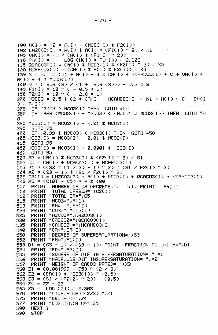
373
100 HCI) = K.2 * A( I > / ( MC03( I > X F2C I > >102 LH2C03C I > = H( I ) * fl< I > X (F1(I> 2> / K1105 OHCI) = KW / (H(I) X (Fl( I > * 2 >)110 PH( I > = - LOG ( FK I ) * F1(D) / 2.303115 QCAC03C I ) = CA( I ) X MC03C I ) * (F2CI) A 2) / K3120 NCR HC03CI) = ( CflC I ) * RC I > * F2C I >) / K4139 S * 0.5 * <N1 + H( I > + 4 * CRCI) + HCRHC03C I > + C + OH< I > + AC I ) + 4 X NCOS's I ) >140 U = C SQR <S) / <1 + SQR (S))) - 0.3 X S 145 F1(I) = 10 C - 0.5 % U)150 F2C I > = 10 A C - 2.0 X U>370 M3C03 = 0.5 X (2 * CRCI) + NCRHC03C I ) + N1 + HC I ) - C - OHC I ) - AC I ) >375 IF M3C03 > MC03CI ) THEN GOTO 490380 IF RBS CMC03CI) - M3C03 > < 03.001 X MC03CI )) THEN GOTO 50 0385 MC03CI> = NC03<I) - 0.01 X MC03CI )395 GOTO 95400 IF (0.99 X M3C03) < NC03CI> THEN GOTO 450 405 MC03CI) = MC03CI) + 0.01 X MC03CI)415 GOTO 95450 NC03CI) * MC03CI) + 0.0001 X MC03CI)460 GOTO 95500502503504505506507 510 512 515 518 520 525 530 535 540 550552553554555556557 560562563564
S3 = CflCI) X MC03CI) * CF2CI) ^ 2) / SI C5 = CRCI) + QCRC03CI ) + NCAHC03CI>XI * ((S3 (1 / 2) - 1 :» 2) X (SI / F2(I) " 2)X2 = (S3 - 1> X (SI /• F2( I > 2)C2(I) = LH2C03CI> + R(I> + MC03CI> + QCRC03CI ) + NCRHC03(I ) X3 * (C1BT - C5) X V X 100 PRINT "NUMBER OF Cfl DECREMENT = 1= PRINT = PRINTPRINT "TOTRL CARBON*'1 ;C2C I )PRINT "TOTAL Cfi*";C5 PRINT "HC03="; fl< I )PRINT "PH= " PH( I )PRINT "C03*";NC03(I>PRINT "H2C03*";LH2C03CI>PRINT "CRCO30-"jQCHC03CI)PRINT "CRHC03+*";NCAHC03( I)PRINT "Cfl+OCflCI)PRINT "DEGREE OF SUPERSflTURflTION*";S3 PRINT "FN="Fl( I >
D1 * (S3 - 1 ) / (S9 - I)' PRINT "FRACTION TO INI S=ODl PRINT "FD=";F2(I )PRINT "SQUARE OF DIF IN SUPERSflTURflTION* 0X1 PRINT "NRCALLOS DIF INSUPERSflTURflTION* 0X2 PRINT "WEIGHT OF CRC03 PPTED* 0X3
Z1 = (0.001999 - C5) * (2 / 3)Z2 = ( CRC I > X MC03( I )) * (0.5)Z3 * (SI / (F2( 0 > 2)) (0.5)Z4 = Z2 - Z3
565 Z5 = LOG (Z4) / 2.303 570 PRINT "(TCAI-TCA )A(2/3 )*";Z1 575 PRINT "DELTA C=OZ4 577 PRINT "LOG DELTA C=OZ5 580 NEXT I590 STOP
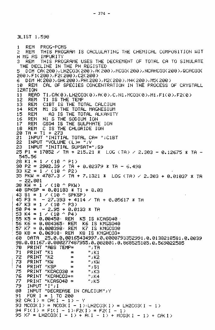
374
JLIST 1,5901 REM PROG-PCMS2 REM THIS PROGRAM IS CRCLULATING THE CHEMICAL COMPOSITION WIT H MG AS IMPURITY3 REM THIS PROGRAMS USES THE DECREMENT OF TOTAL CA TO SIMULATE THE DECLINE IN THE PH REGISTED
5 DIM CA<208>,LH2C03<200 ),AC 200>,MC03C200>, NCAHC03C200>,QCAC03C 200 >, F1C 200 >, F2C 200 >, C2C 200 >6 DIM HC200>,OHC200 >,PHC 200>,M2C200>,M4C200>,M5C200 >10 REM CAL OF SPECIES CONCENTRATION IN THE PROCESS OF CRYSTALL IZATION11 READ T1,CAC 0 ),LH2C03C0 >,AC 0 >,C,N1,MC03C0 >,M1,F1<0>,F2C0>12 REM T1 IS THE TEMP13 REM C1BT IS THE TOTAL CALCIUM14 REM Ml IS THE TOTAL MAGNESIUM15 REM A3 IS THE TOTAL ALLANITY16 REM N1 S THE SODIUM ION17 REM GS04 IS THE SULPHATE ION18 REM C IS THE CHLORIDE ION20 TA = T1 + 27321 INPUT "INITIAL TOTAL CA= ";C1BT22 INPUT "VOLUME C L >= ";V23 INPUT "INITIAL SUPSAT=";S925 PI = 17052 / TA + 215.21 X LOG C TA > / 2.303 - 0.12675 X. TA - 545.56
28 K1 = 1 / <10 PI)30 P2 = 2902.39 ✓ TA + 0.02379 X TA - 6.438 33 K2 = 1 / <10 '' P2>35 PKW = 4787.3 / TA + 7.1321 X LOG CTA> / 2.303 + 0.01037 X TA - 22.801
38 KW a 1 / <10A PKW )40 SPKSP = 0.01183 X T1 + 8.0343454750
SIP3K3P4
1 / (10- 27.393
1 / < 10- 2.95 +
SPKSP >+ 4114P3)0.0133
/ TA + 0.05617 X TA X TA
! 53 K4 = 1 / <10 A■ P4>55 K5 s 0.00450= REM K5 IS KCASO40
| 56 K6 a 0.004365= REM K6 IS KMGSO40! 57 K7 a 0.000398= REM K7 IS KMGCO3058 K8 = 0.06918: REM K8 IS KMGHC03+60 DATA 25.0,0.00165434997,0.0000793352991,0.0138218581,0.0039 98,0.01167,0.000277487355,0.002001,0.868525105,0.56302258570 PRINT "ABS TEMP= "; TA71 PRINT "K1 "; K172 PRINT "K2 "; K273 PRINT "KW "; KW74 PRINT "KSP ";S175 PRINT "KCACO30 = "; K376 PRINT "KCAHC03+= "; K4
PRINT "KCASO40 = "; K579 INPUT " I.. . I80 INPUT "DECREASE IN CALCIUM";Y91 FOR I = 1 TO 20092 CACI) = CACI - 1 ) - Y93 MC03CI ) = MC03CI - 1 ):LH2C03CI> = LH2C03CI - 1 >94 F1 < I > = F1 < I - 1):F2<I) = F2C I - 1)95 X7 = LH2C03C I - 1 > + AC I - 1 > + MC03C 1-1) 4 CAC I >
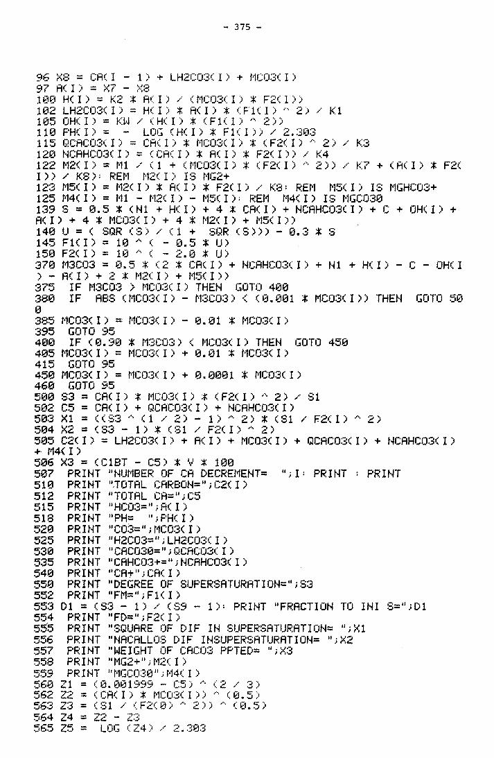
375
96 X8 = Cfl( I - 1 ) + LH2C03C I > + MC03( I )q? j •, = _ yft
100 H( I > = K2 * fl( I > -••• < MC03C I > * F2C 1 )>102 LH2C03C I ) = H(I) * fl( 1 ) % (F1(I) rt 2) / K1105 OHU) = KW / (H(I) * (F1(I) 2>>110 PHCI) = - LOG CH< I > X F1(D) ✓ 2.303115 QCAC03C I ) = CflC I > * MC03CI ) % C F2C I) A 2) / K3120 NCAHC03( I ) = (CAU) * fl( I ) % F2(I)) / K4122 M2( I > = Ml / (1 + < MC03C I ) t < F2C I > A 2>> / K7 + (H(I) * F2<I)) / K8) = REM M2( I ) IS MG2+123 M5( I ) = M2< I ) % H(I) X F2<I > / K8* REM M5( I ) IS MGHC03+125 M4(I> = Ml - M2(I ) - M5(I): REM M4CI ) IS MGCO30139 3 = 0.5 X C N1 + HU) + 4 X CflC I > + NCAHC03C I ) + C + OHCI ) +AU ) + 4 X MC03C I ) + 4 * M2C I > + M5C I ))140 IJ = < SQR CS ) / <1 + SQR (3 ) ) ) - 0.3 X 3145 F1CI) = 10 C - 0.5 X IJ)150 F2(I) = 10 C - 2.0 X U>370 M3C03 = 0.5 X (2 X CflC I ) + NCRHC03C I ) + N1 + H(I) - C - OHU ) - RC I ) + 2 X M2C I ) + M5C I ) )375 IF M3C03 > MC03CI ) THEN GOTO 400380 IF RB3 CMC03CI) - M3C03) < (0,001 X MCQ3CI )) THEM GOTO 50 0385 MC03CI ) = MC03CI) - 0.01 X MC03CI )395 GOTO 95400 IF (0.90 X M3C03) < MC03CI> THEN GOTO 450 405 MC03CI) = MC03(I ) + 0.01 X MC03(I )415 GOTO 95450 MC03(I) = MC03(I ) + 0.0001 X MC03(I )460 GOTO 95500 S3 = CA( I ') X MC03 (I) X (F2( I ) * 2) ✓ 31502 C5 = CR(I ) + QCRC03(I ) + NCRHC03CI)503 XI = ((S3 (1 / 2) - 1 ) 2) X (31 / F2< I ) ^ 2)504 X2 * (S3 - 1) X (SI / F2CI) A 2)505 C2(I ) = LH2C03(I ) + R(I ) + MC03(I ) + QCHC03CI ) + NCRHC03(I ) + M4( I )506507 510 512 515 518 520 525 530 535 540 550552553554555556557558559
X3 = (C1BT - C5) X V X 100 PRINT "NUMBER OF OR DECREMENT* "; I= PRINT * PRINT PRINT "TOTAL CARBON*";C2(I )PRINT "TOTAL Cfl=";C5 PRINT "HC03=";ACI )PRINT "PH= " PH( I )PRINT "C03=";MC03(I )PRINT "H2C03=";LH2C03CI )PRINT "CRCO30*";QCRC03CI )PRINT "CRHC03+=";NCRHC03CI )PRINT "CR+"CR( I )PRINT "DEGREE OF SUPERSRTURRTION=";S3 PRINT "FM=";F1(I )
D1 = (S3 - 1) / (S9 - 1): PRINT "FRACTION TO INI S=";D1 PRINT "FD="iF2(I )PRINT "SQUARE OF DIF IN SUPERSATURATION= ";X1 PRINT "NACALLOS DIF INSUPERSATURATION= "X2 PRINT "WEIGHT OF CAC03 PPTED= ";X3 PRINT "MG2+";M2(I )PRINT "MGCO30" :> M4( I )
560 Z1 = (0.001999 - 05) A (2 / 3)562 Z2 = (CA( I ) X MC03CI)) A (0-5)563 Z3 = (31 / (F2(0) * 2)) * (0.5)564 Z4 = Z2 - Z3565 Z5 = LOG (Z4) 2.303
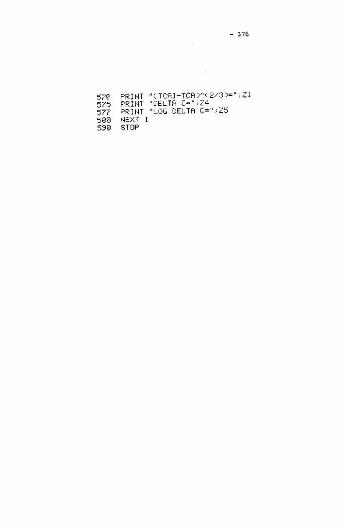
376
570 PRINT "C TCfiI-TCP X'<2/3>="J21 575 PRINT "DELTA C=";24 577 PRINT "LUG DELTA C=";Z5 580 NEXT I 590 STOP

- 377 -
JXIXI:jlist
10 RREN ^HiYisShE PROGRAM TO CALCULATE THE SURFACE AREA OF CA
523 pFMEDnN NUMBER DISTRIBUTION BY DECREMEHTAL SIZE REDUCTION FR OM THE FINAL CRYSTAL SIZE REDUCTION FROM THE FINAL cRrSTAL NUMBE
R0C1REMIBTHE SURFACE AREA AND THE WEIGH! OF URYSfALB DURING CRio
I0LLrImTIBACKWARDLTO ENABLE^RATE OF CRYSTALLIZATION CALCULATION60 DIM NC 100 >) DC 100 >61 626566 70757677
DIM AC 100 )> WC 100)DIM EC 100 > „INPUT "SURFACE SHAPE FACTOR "jFI INPUT "VOLUME SHAPE FACTOR INPUT "SIZE DECREMENT ";X
REM M IS THE NUMBER
i F2
M = 18 OF DATA PAIR
AREA"i ThBC 25); "TOTAL WEIGHT"; T
?T ®TfiBt 50); "BASED 0N NUMBER"- PRINT80 FOR I = 1 TO M85 READ NCI), DC I)93 DATA 93) 194 DATA 133.. 3. 195 DATA 84,. 5- 196 DATA 62)7.297 DATA 128)9.298 DATA 59)11.399 DATA 94)13.3100 DATA 53)15.3101 DATA 59.. 17.4102 DATA 88)19.4103 DATA 81)21.5104 DATA 80)23.5105 DATA 81)25.6106 DATA 74)27.6107 DATA 82)29.7108 DATA 71)31.7109 DATA 46..33.81 10 DATA 24)35.8200 NEXT I205 SUMA = 0206 WSUM = 0208 GSUM = 0209 QSUM = 0211 FOR I = 1 TO M212 IF DC I) < 0 THEN215 AC I > = FI * NC I > *216 WC I > = F2 % 2. 71 *217 EC I > = DC I > X NC I )220 SUMA = SUMA + AC I >221 WSUM = WSUM + wc r >222 GSUM = GSUM + NC I )223 QSUM = QSUM + m V
226 NEXT‘ I230 SUMA = SUMA X c 10
GOTO 226C DC I > 2 >He I) I (DC I > 3>
C - 8 >> * HI
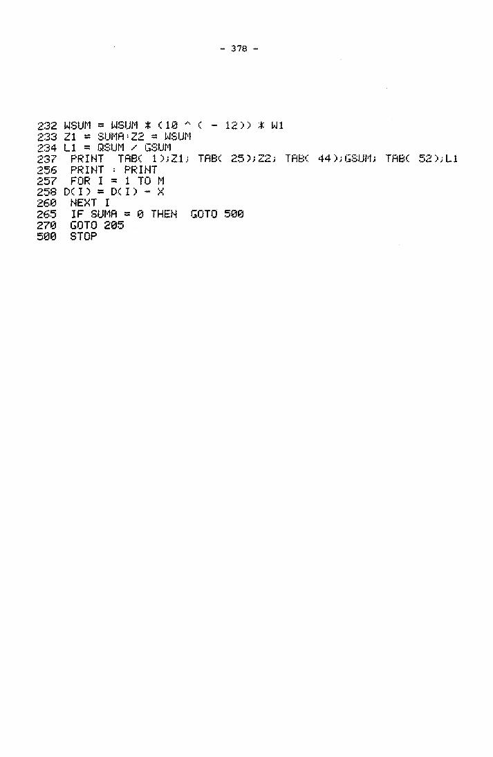
378
232 WSUM = WSUM t (. 10 ( - 12 >> * W1233 Z1 = SUMfl:Z2 = WSUM234 LI = QSUM / GSUM23? PRINT TflBC 1>;Z1; TflBC 25>;Z2; TRB( 44); GSUM; TftBC 52);L1256 PRINT : PRINT257 FOR I = 1 TO M 253 D< I > a D< I ) - X 260 NEXT I265 IF SUMfl = 0 THEN GOTO 500 270 GOTO 205 500 STOP
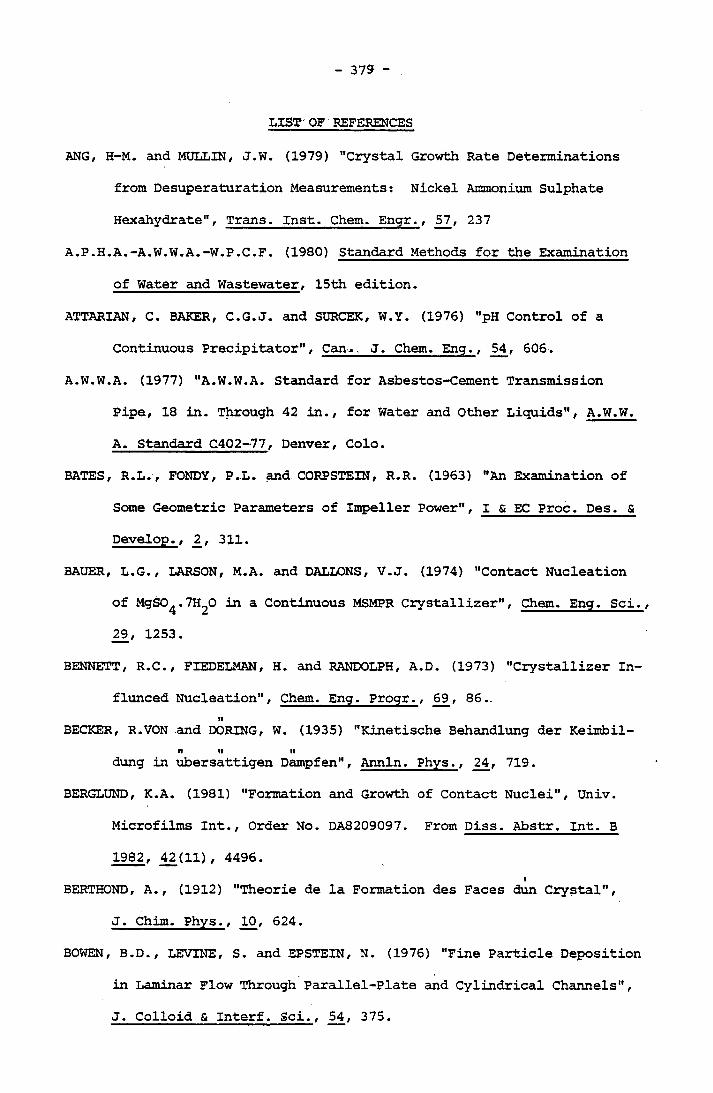
- 379 -
LIST OF REFERENCES
ANG, H-M. and MULLIN, J.W. (1979) "Crystal Growth Rate Determinations from Desuperaturation Measurements: Nickel Ammonium Sulphate
Hexahydrate", Trans. Inst. Chem. Engr., 57, 237A.P.H.A.-A.W.W.A.-W.P.C.F. (1980) Standard Methods for the Examination
of Water and Wastewater, 15th edition.
ATTARIAN, C. BAKER, C.G.J. and SURCEK, W.Y. (1976) "pH Control of a Continuous Precipitator", Can,.. J. Chem. Eng., 54, 606.
A.W.W.A. (1977) "A.W.W.A. Standard for Asbestos-Cement TransmissionPipe, 18 in. Through 42 in., for Water and Other Liquids", A.W.W.A. Standard C402-77, Denver, Colo.
BATES, R.L., FONDY, P.L. and CORPSTEIN, R.R. (1963) "An Examination of
Some Geometric Parameters of Impeller Power", I & EC Proc. Des. & Develop., 2_, 311.
BAUER, L.G., LARSON, M.A. and DALLONS, V.J. (1974) "Contact Nucleationof MgSO^.7H^O in a Continuous MSMPR Crystallizer", Chem. Eng. Sci., 29, 1253.
BENNETT, R.C., FIEDELMAN, H. and RANDOLPH, A.D. (1973) "Crystallizer In- flunced Nucleation", Chem. Eng. Progr., 69, 86.
ItBECKER, R.VON and DORING, W. (1935) "Kinetische Behandlung der Keimbil-
It It Itdung in ubersattigen Dampfen", Annin. Phys., 24, 719.
BERGLUND, K.A. (1981) "Formation and Growth of Contact Nuclei", Univ. Microfilms Int., Order No. DA8209097. From Piss. Abstr. Int. B 1982, 42(11), 4496.
IBERTHOND, A., (1912) "Theorie de la Formation des Faces dun Crystal",J. Chim. Phys., 10, 624.
BOWEN, B.D., LEVINE, S. and EPSTEIN, N. (1976) "Fine Particle Deposition in Laminar Flow Through Parallel-Plate and Cylindrical Channels",J. Colloid & Interf. Sci., 54, 375.
380
BROOKS, R., CLARK, L.M. and THURSTON, E.R. (1950) "CaC03 and its Hydrates", Trans. Roy. Soc. London, A243, 145.
BUCKLEY, H.E. (1951) Crystal Growth, John Wiley and Sons Ltd.
BURTON, W.K., CABRERA, N. and FRANK, F.C. (1951) "The Growth of Cry
stals and the Equilibrium Structure of their Surfaces", Phil.
Trans., A243, 299.
CABLE, M. and EVANS, D.J. (1967) "Spherically Symmetrical Diffusion- Controlled Growth or Dissolution of a Sphere", J. App. Phys.,38, 2899.
CARDEW, D.T. (1982) "Crystal Growth Rates from Batch Experiments",J. Cryst. Growth, 57, 391.
CHANDLER, J.L. (1964) "The Effect of Supersaturation and Flow Conditions on the Initiation of Scale Formation", Trans. Inst. Chem. Engr., 42, 724.
CHERNOV, A.A. (1961) "The Spiral Growth of Crystals", Soviet Phys.Usp., £, 116.
CHRISTIANSEN, J.A. and NIELSEN, A.E. (1951) "Kinetic Determination ofthe Size of Crystal Germs", Acta Chem. Scand., _5, 674.
CHRISTIANSEN, J.A. (1954) "On Attainment of the Stationary (Steady)State in Nucleation", Acta Chem. Scand., 8_, 909.
CISE, M.D. and RANDOLPH, A.D. (1972) "Secondary Nucleation of PotassiumSulphate in a Continuous Flow Seeded Crystallizer", A.I.Ch.E.Symp. Ser., 6£(121), 42.
CLONTZ, N.A. and McCabe, W.L. (1971) "Contact Nucleation of Magnesium Sulphate Heptahydrate", A.I.Ch.E. Symp. Ser., 6_7(110) , 6.
COATES, K.E. and KNUDSEN, J.G. (1980) "Calcium Carbonate Scaling Characteristic of Cooling Tower Water". ASHRAE Trans., 86, part 2, 68.
DAHNEKE, B. (1973) "Measurements of Bouncing of Small Latex Spheres",J. Colloid & Interf. Sci., 45 , 584.
381
DAVIES, C.W. and JONES, A.L. (1955) "The Precipitation of Silver
Chloride from Aqueous Solutions", Trans. Faraday Soc., _51, 812.DAVIES, C.W. (1967) Electrochemistry, George Newnes Ltd., London.DE BOER, J.H. (1968) The Dynamical Character of Adsorption, Clanen-
don Press, Oxford.DIEHL, H., GOETZ, C. and HACH, C. (1950) "Determination of Calcium and
Determination of the Total Hardness of Water", J. Am. Wat. Wks. Assoc., 42, 40.
DOREMUS, R.H. (1958) "Precipitation Kinetics of Ionic Salts from Solu
tions", J. Phys. Chem., 62, 1068.DOREMUS, R.H. (1970) "Crystallization of Slightly Soluble Salts from
Solutions", J. Phys. Chem., 74, 1405.DYE, J.F. (1952) "Calculations of the Effect of Temperature on pH, Free
Carbon Dioxide and the Three Forms of Alkalinity", J. Am. Wat.Wks. Assoc., 44, 356.
ENCYLOPEDIA BRITANNICA (1984) Encyclopedia Britannica, William Benton Publisher, 3_, p.833.
FEITLER, H. (1972) "Cooling Water Scale Control: The Scale Meter andthe Critical pH of Scaling", Mat. Prot. & Perf., 11, 29.
FEITLER, H. (1974) "The Effect of Scaling Indexes on Cooling Water Treatment Practice", 35th Annual Meeting, International Water Conference, Paper No. IWC74-21, October, Pittsburgh, Pa.
FEITLER, H. (1975) "Critical pH Scaling Indexes", Mat. Prot. & Perf.,
14, 33.FISCHER, P., SUITOR, J.W. and RITTER, R.B. (1975) "Fouling Measurement
Techniques", Chem. Eng. Progr., 77, 66.FRANK, F.C. (1949) "The Influence of Dislocations on Crystal Growth",
Symposium on Crystal Growth, Discuss. Faraday Soc., No. 5, 48.FRISCH, H.L. and COLLINS, F.C. (1952) "Diffusional Processes in the
Growth of Aerosol Particles", J. Chem. Phys., 20, 1797.

382
FRISCH, H.L. and COLLINS, F.C. (1953) "Diffusional Processes in the Growth of Aerosol Particles", J. Chem. Phys., 21, 2158.
GARRELS, R.M. and THOMPSON, M.E. (1962) "A Chemical Model for Sea Water at 25°C and One Atmospheric Total Pressure", Am. J. Sci., 260, 57.
GARSIDE, J. (1971) " The Concept of Effectiveness Factors in Crystal Growth", Chem. Eng. Sci., 26, 1425.
GARSIDE, J. and LARSON, M.A. (1978) "Direct Observation of Secondary Nuclei Production", J. Cryst. Growth, 43, 694.
GARSIDE, J., RUSLI, I.T. and LARSON, M.A. (1979) "Origin and Size Distri bution of Secondary Nuclei", A.I.Ch.E. J., 25, 57.
GAZIT, E. and HASSON, D. (1975) "Scale Deposition from an Evaporating Falling Film", Desalination, 17, 339.
GIBBS, J.W. (1928) "On the Equilibrium of Heterogeneous Substances",Vol. 1, Collected Works, Longmans.
GOLDSTEIN, M. (1968) "Interparticle Interference Effects in Diffusion Controlled Growth", J. Cryst. Growth, 3/4, 594.
GOUJON, G, and MUTAFTSCHIEV, B. (1976) "On Some Energetic and ChemicalProperties of the Calcite Surface. A. Heat of Immersion in Water", J. Chim. Physique, 73, 351.
HAM, F.S. (1958) "Theory of Diffusion-limited Precipitation", Phys.Chem. Solids, 6_, 335.
HARNED, H.S. and HAMER, W.J. (1933)"Ionization Constant of Water and the
Dissociation of Water in Potassium Chloride Solutions from Electromotive Forces of Cells Without Liquid Junctions", J. Am. Chem.
Soc,, 55, 2194.HARNED, H.S. and DAVIS, R. (1943) "The Ionization Constant of Carbonic
Acid in Water and the Solubility of Carbon Dioxide in Water and Aqueous Salt Solution from 0 to 50°C", J. Am. Chem. Soc., 65, 2030
383
HARNED, H.S. and SCHOLES, S.R. (1943) "The Ionization Constant of
HCO^ from 0 to 50°C"/ J. Am. Chem. Soc., 63,1706.HASSON, D (1962) "Rate of Decrease of Heat Transfer due to Scale Depo
sition", Dechema-Monographien, 47, 233.
HASSON, D., AVRIEL, M., RESNICK, W., ROZENMAN, T. and WINDREICH, S.(1968) "Mechanism of Calcium Carbonate Scale Deposition on Heat Transfer Surfaces", I & EC Fundam., 1_, 59.
HASSON, D., SHERMAN, H. and BITON, M. (1978) "Prediction of Calcium
Carbonate Scaling Rates", 6th Intern. Symp. Fresh Water from
the Sea, 193.HAWTHORN, D. and PERRY, D.J. (1980) "The Fouling of Power Station Con
denser Tubes by Tricalcium Phosphate", Eff. & Water Treat. J.,20, 77.
HEAT EXCHANGER INSTITUTE (1978) Standards for Steam Surface Condensers, p.6, 7th Edition.
HILTON, H. (1903) Mathematical Crystallography, Oxford.HOUSE, W.A. and TUTTON, J.A. (1982) "An Investigation of the Heteroge
neous Nucleation of Calcite", J. Cryst. Growth, 56, 699.HOUSE, W.A. (1981) "Kinetics of Crystallization of Calcite from Calci
um Bicarbonate Solutions", J. Chem. Soc. Faraday Trans. I, 77, 341.HULBURT, H.M. and KATZ, S. (1964) "Some Problems in Particle Technology:
a Statistical Mechanical Formation", Chem. Eng. Sci., 19, 555.
JACOBSON, R.L. and LANGNUIR, D. (1974) "Dissociation Constants of Calcite and CaHCO* from 0 to 50°C", Geochim. Cosmochim. Acta, 38, 301.
JOHNSON, G.W. (1950) "Some Observations on the Epitaxy of Sodium Chloride on Silver", J. App. Phys., 21, 1057.
JOHNSON, G.W. (1951) "The Epitaxy of Alkali Chlorides on Metals", J♦ App.
Phys., 22, 797.
384
JOHNSON, R.T., ROUSSEAU, R.W. and McCABE, W.L. (1972) "Factors Affecting Cantact Nucleation". A.I.Ch.E. Sym. Ser., 68_(121), 31.
JOHNSTONE, R.E. and THRING, M.W. (1957) Pilot Plants, Models and Scale- up Methods in Chemical Engineering, McGraw-Hill, New York.
KAHLWEIT, M. (1960) "Kinetics of Phase Formation in Condensed Systems.
(Precipitation of Difficulty Soluble Electrolytes from Aqueous Solutions). ", Z. Physik. Chem. N. F., 25, 125.
KAZMIERCZAK, T.F. (1979) Ph.D. Thesis, State University of New York, Buffalo.
KAZMLERCZAK, T.F., TOMSON, M.B. and NANCOLLAS, G.H. (1982) "Crystal Growth of Calcium Carbonate. A Controlled Composition Kinetic Study", J. Phys. Chem., 86, 103.
KERN, D.Q. and SEATON, R.E. (1959) "A Theoretical Analysis of Thermal Surface Fouling", Br. Chem. Eng., _4, 258.
KHAMSKII, E.V. (1969) Crystallization from Solutions, Consultants Bureau, New York, London.
KHARIN, V.M. (1974) "Kinetics of the Crystallization of Polymorphic Modifications of Calcium Carbonate", Zh. Fiz. Khim., 48, 1724.
KHARIN, V.M., KOSOVTSEVA, A.V. and DOBROMIROVA, V.F. (1980) "Analysis of the Kinetics of Crystal Nucleation and Growth in Solutions", Translated from Teore. Osn. Khim. Tekhnologii, 14, 364.
KITANO, Y. (1962) "Calcium Carbonate Crystals Forms formed from Sea Water by Inorganic Processes", J. Oceanogr. Soc. Japan, 18, 35.
KITANO, Y. and HOOD, D.W. (1965) "The Influence of Organic Material on the Polymorphic Crystallization of Calcium Carbonate", Geochim. Cosmochim. Acta, 29, 29.
KITANO, Y. (1966) "Synthesis of Magnesian Calcite at Low Temperatures and Pressures", Geochim. J. (Nagoya), 1, 1.
385
KNUDSEN, J.G. and STORY, M. (1975) "The Effect of Heat Transfer Surface Temperature on the Scaling Behavior of Simulated Cooling Tower Water", A.I.Ch.E. Sym. Ser., 74(174), 26.
KONAK, A.R. (1971) "The Crystallization and Dissolution of Gypsum", Ph.D.
Thesis, The University of Birmingham.KONAK, A.R. (1974) "A New Model for Surface Reaction-controlled Growth of
Crystals from Solution", Chem. Eng. Sci., 29, 1537.It II
KOSSEL, W. (1934) "Zur Energetik von Oberflachenvorgangen", Annin. Phys.,
21, 457.LAL, D.P., MASON, R.E.A. and STRICKLAND-CONSTABLE, R.F. (1969) "Collision
Breeding of Nuclei", J. Cryst. Growth, _5, 1.LANGMUIR, D. (1968) "Stability of Calcite Based on Aqueous Solubility
Measurements", Geochim. Cosmochim. Acta, 32, 835.LARSON, M.A. (1982) "Secondary Nucleation: An Analysis", in Industrial
Crystallization 81, edited by Jancic, S.J. and De Jong, E.J., North- Holland Publishing Company, 55.
LARSON, T.E. and BUSWELL, A.M. (1942) "Calcium Carbonate Saturation Index and Alkalinity Interpretation", J. Am. Wat. Wks. Assoc., 34, 1667.
LEE, S.H. and KNUDSEN, J.G. (1978) "Scaling Characteristics of Cooling Tower Water", ASHRAE Trans., 85, part I.
LIESER, K.H. (1969) "Steps in Precipitation Reactions", Angew. Chem. In- ternat. Edit., 8_, 188.
LINTON, W.H. and SHERWOOD, T.K. (1950) "Mass Transfer from Solid Shapes
to Water in Streamline and Turbulent Flow", Chem. Eng. Progr., 46,258.
LITTLE, S. (1984) Personal Communication, Electricity Commission of New
South Wales.LOEWENTHALL, R.E. and MARAIS, G.v.R. (1976) Carbonate Chemistry of Aquatic
Systems: Theory and Application, Ann Arbor Publishers, Ann Arbor.

386
McCABE, W.L. and ROBINSON, C.S. (1924) "Evaporator Scale Formation",Ind. Eng. Chem., 16, 478.
McCABE, W.L. and SMITH, J.C. (1967) Unit Operations of Chemical Engi
neering, p.336, McGraws-Hill Book Co., Inc., N.Y.fl tl II
MARC, R. (1908) "Uber die Kristallisation aus wasserigen Losurgen",Z. Phys. Chem., 61, 385.
MARUSCAK, A, BAKER, C.G.J. and BERGOUGNOU, M.A. (1971) "Calcium Carbonate Precipitation in a Continuous Stirred Tank Reactor", Cand.
J. Chem. Eng., 49, 819.MASON, R.E.A. and STRICKLAND-CONSTABLE, R.F. (1966) "Breeding of Crys
tal Nuclei", Trans. Faraday Soc., 62, 455.
MELIA, T.P. and MOFFITT, W.P. (1964) "Secondary Nucleation from Aqueous Solution", I & EC Fundam. , 3_, 313.
MELIA, T.P. (1965) "Crystal Nucleation from Aqueous Solution", J. App♦ Chem., 15, 345.
MERRILL, D.T. (1976) "Chemical Conditioning for Water Treatment and Corrosion Control", Water Treatment Plant Design, edited by Sanks, R. L,, Ann Arbor Science Publ., Ann Arbor, Mich.
MERRILL, D.T. and Sanks, R.L. (1977a) "Corrosion Control by Deposition
of CaCO^ Films: A Practical Approach for Plant Operators", J. Am.Wat. Wks. Assoc., 69, 592.
MERRILL, D.T. and SANKS, R.L. (1977b) "Corrosion Control By Deposition
of CaCO^ Films: A Practical Approach for Plant Operators", J. Am.Wat. Wks. Assoc., 69, 634.
MERRILL, D.T. and SANKS, R.L. (1978) "Corrosion Control by Deposition of CaCO^ Films: A Practical Approach for Plant Operators", J. Am.Wat. Wks. Assoc., 70, 12.
MIERS, H.A. and ISAAC, F. (1906) "Refractive Indices of Crystallizing Solutions", J. Chem. Soc., 89, 413.

387
MOLLER, P. and RAJAGOPALAN, G. (1975) "Precipitation Kinetics of CaC032+ "in Presence of Mg Ions", Zeit. fur Phys. Chem. Neue Folge, Bd.
94, S.297.II
MOLLER, P. and RAJAGOPALAN, G. (1976) "Changes of Excess Free Energiesin the Crystal Growth Processes of Calcite and Aragonite due to
2+ "the Presence of Mg Ions in Solution", Zeit. fur Phys. Chem.Neue Folge, Bd.99, S.187.
MORSE, R.W. and KNUDSEN, J.G. (1977) "Effect of Alkalinity on the Scaling of Simulated Cooling Tower Water", Can. J. Chem. Eng., 55, 272.
MULLIN, J.W. and RAVEN, K.D. (1961) "Nucleation in Agitated Solutions", Nature, 4772, 251.
MULLIN, J.W. (1972) Crystallization, Butterworths, London.MULLIN, J.W. and OSMAN, M.M. (1973) "Nucleation and Precipitation of Nic
kel Ammonium Sulphate Crystals from Aqueous Solution", Krist. Tech., 8, 471.
MULLIN, H.W. and ANG, H-M. (1977) "Nucleation Characteristics of Aqueous Nickel Ammonium Sulphate Solutions", Krist. Tech., 12, 105.
NANCOLLAS, G.H. and REDDY, M.M. (1971) "The Crystallization of Calcium Carbonate II. Calcite Growth Mechanism", J. Colloid Interf. Sci.,37, 824.
NERNST, W. (1904) "Theorie der Reaktions Geschwindigkeit in Heterogenen Systemen", Z. Phys. Chem., 47, 52.
NEWKIRK, and TURNBULL, D. (1955) "Nucleation of Ammonium Iodide Crystals
from Aqueous Solutions", J. App. Phys., 26, 579.
NIELSEN, A.E. (1955) "The Kinetics of Electrolyte Precipitation", J. Colloid Sci., 10, 576.
NIELSEN, A.E. (1964) Kinetics of Precipitation, Pergamon Press, London.
388
NIELSEN, A.E. (1967) "Nucleation in Aqueous Solution", Crystal Growth,
Edited by Peiser, Pergamon, Oxford.NIELSEN, A.E. (1969) "Nucleation and Growth of Crystals at High Super--
saturation", Krist. Teck., 4_, 17.
NIELSEN, A.E. (1982) "Theory of Electrolytic Crystal Growth" in Indus-I
trial Crystallization 81, edited by Jancic, S.J. and De Jong, E. J., North-Hallard Publishing Company, 35.
IfNIELSEN, A.E. and SOHNEL, 0. (1971) "Interfacial Tensions Electrolyte
Crystal-Aqueous Solution from Nucleation Data", J. Cryst. Growth, 11, 233.
NOYES, A.A. and WHITNEY, W.R. (1897a) "Rate of Solution of Solid Substances in their Own Solution", J. Am. Chem. Soc., 19, 930.
NOYES, A.A. and WHITNEY, W.R. (1897b) "Rate of Solution of Solid Substances in their Own Solution", Z. Phys. Chem., 23, 689.
INYVLT, J. (1968) "Kinetics of Nucleation in Solutions", J. Cryst. Growth, 3/4, 377.
O'ROURKE, J.D. and JOHNSON, R.A. (1955) "Kinetics and Mechamism in Formation of Slightly Soluble Ionic Precipitates", Anal. Chem., 27, 1699.
OHARA, M. and REID, R.C. (1973) Modeling Crystal Growth Rates from Solution , Prentice-Hall, Inc., N.J.
OLSON, R.M. (1973) Essentials of Engineering Fluid Mechanics, pp.356-357
Intext Educational Publishers, N.Y.OTTENS, E.P.K., JANSE, A.E. and DE JONG, E.J. (1972) "Secondary Nuclea
tion in a Stirred Vessel Cooling Crystallizer", J. Cryst. Growth, 13/14, 500.
PINCUS, L.I. (1962) Practical Boiler Water Treatment, P.227, McGraw-Hill Book Co., Inc., New York.
389
PLUMMER, L.N. and WIGLEY, T.M.L. (1976) "The Dissolution of Calcite in CO^-saturated Solution at 25°C and 1 Atmosphere Total Pressure",
Geochim. Cosmochim. Acta, 40, 191.
PLUMMER, L.N., WIGLEY, T.M.L. and PARKHURST, D.L. (1978) "The Kinetics of Calcite Dissolution in CC^-water Systems at 5° to 60°C and 0.0to 1.0 Atm. CCV, Am. J. Sci., 278, 179.Z --- ---
PLUMMER, L.N., PARKHURST, D.L. and WIGLEY, T.M.L. (1979) "Critical Review of the Kinetics of Calcite Dissolution and Precipitation", in Chemical Modeling in Aqueous Systems, edited by Jenne, E.A. (American Chemical Society Symposium Series), 93_, 537.
POUND, G.M. and LA MER, V.K. (1952) "Kinetics of Crystalline NucleusFormation in Supercooled Liquid Tin", J♦ Am. Chem. Soc., 74, 2323.
PYTKOWICA, R.M. (1965) "Rates of Inorganic Calcium Carbonate Nucleation", J. Goel., 73, 196.
RANDOLPH, A.D. (1964) "A Population Balance for Countable Entities", Can.J. Chem. Eng., 42, 280.
RANDOLPH, A.D. and CISE, M.D. (1972) "Nucleation Kinetics of the Potassium Sulphate-Water System", A.I.Ch.E. J., 18, 798..
RANDOLPH, A.D. and LARSON, M.A. (1971) Theory of Particulate Process -Analysis and Techniques of Continuous Crystallization, Academic Press, N.Y.
RANDOLPH, A.D. and SIKDAR, S.K. (1976) "Creation and Survival of Secondary Crystal Nuclei. The Postassium Sulphate-Water System", I & EC Fundam., 15, 64.
REARDON, E.J. and LANGMUIR, D. (1974) "Thermodynamic Properties of the
Ion Pairs MgC0° and'CaCO® from 10 to 50°C", Am. J. Sc., 274, 599.REDDY, M.M. (1977) "Crystallization of Calcium Carbonate in the Presence
of Trace Concentrations of Phosphorus-containing Anions", J. Cryst.

390
Growth, _41, 287.REDDY, M.M. and GAILLARD, W.D. (1981) "Kinetics of Calcium Carbonate
(Calcite)-seeded Crystallization: Influence of Solide/Solution
Ratio on the Reaction Rate Constant", J. Colloid Interf. Sci.,
81, 171.REDDY, M.M. and NANCOLLAS, G.H. (1971) "The Crystallization Calcium
Carbonate I. Isotopic Exchange and Kinetics", J. Colloid Interf.Sci., 36, 166.
REDDY, M.M. and NANCOLLAS, G.H. (1973) "Calcite Crystal Growth Inhibition by Phosphonates", Desalination, 12, 61.
REDDY, M.A. and NANCOLLAS, G.H. (1976) "The Crystallization of CalciumCarbonate IV. The Effect of Magnesium, Strotium and Sulphate Ions", J. Cryst. Growth, 35, 33.
REDDYM M.M., PLUMMER, L.N. and BUSENBERG, E. (1981) "Crystal Growth ofCalcite from Calcium Bicarbonate Solutions at Constant P and
co225°C: A Test of a Calcite Dissolution Model", Geochim. Cosmochim.Acta, 45, 1281.
REDDY, M.M. and WANG, K.K. (1980) "Crystallization of Calcium Carbonate in the Presence of Metal Ions. I. Inhibition by Magnesium Ions at pH 8.8 and 25°C", J. Cryst. Growth, 50, 470.
REITZER, B.J. (1964) "Rate of Scale Formation in Tubular Heat Exchanger", I & EC Proc. Des. & Develop., 3_, 345.
ROQUES, H. and GIROU, A. (1974) "Kinetics of the Formation Conditions of Carbonate Tartars", Wat. Res., £3, 907.
ROSSUM, J.R. and MERRILL, D.T. (1983) "An Evaluation of the Calcium Carbonate Saturation Indexes", J. Am. Wat. Wks. Assoc., 72, 95.
RUCKENSTEIN, E. and PRIEVE, D.C. (1973) "Rate of Deposition of Brownian Particles under the Action of London and Double-layer Forces",J. Chem. Soc. Faraday II, 69, 1522.
391
RUSLI, I.T., LARSON, M.A. and GARSIDE, J. (1980) "Crystallization. Ini
tial Growth of Secondary Nuclei Produced by Contact Nucleation",
CEP Sym. Ser., 76^(193), 52.
RUSHTON, J.H., COSTICH, E.W. and EVERETT, H.J. (1950a) "Power Characte
ristics of Mixing Impellers, Part I", Chem. Eng. Progr., 46, 395.
RUSHTON, J.H., COSTICH, E.W. and EVERETT, H.J. (1950b) "Power Characte
ristics of Mixing Impellers, Part II", Chem. Eng. Progr., 46, 467.
RYZNAR, J.W. (1944) "A New Index for Determining Amount of Calcium Car
bonate Scale Formed by a Water", J. Am. Wat. Wks. Assoc., 36, 472.
SCHIERHOLZ, P. and STEVENS, J.D. (1975) "Determination of the Kinetics
of Precipitation in a Dilute System", A.I.Ch.E. Sym. Ser., 71 (151),
249.
SNOEYINK, V.L. and JENKINS, D. (1980) Water Chemistry, John Wiley and
Sons, New York.If
SOHNEL, 0 and MULLIN, J.W. (1978) "A Method for the Determination of Pre
cipitation Induction Periods", J. Cryst. Growth, 44, 377.If
SOHNEL, 0. and MULLIN, J.W. (1982) "Precipitation of Calcium Carbonate",
J. Cryst. Growth, 60, 239.
SOMERSCALES, E.F.C. (1979) "Introduction and Summary: The Fouling of
Heat Transfer Equipments", Int. Conf. on the Fouling of Heat Tran
sfer Equipment, Troy, New York.
SPIELMAN, L.A. and FRIEDLANDER, S.K. (1974) "Role of the Electrical Dou
ble Layer in Particle Deposition by Convective Diffusion", J. Col
loid Interf. Sci., 46, 22.
STEINBERG, S. and HASSON, D. (1979) "Analysis of the Effect of Brine Re
tention Time on the Scaling Potential", Desalination, 31, 267.
STRANSKI, I.N. (1928) "Zur Theorie des Kristallwachsturns", Z. Phys. Chem.,
136, 259.
392
STRANSKI, I.N. (1930) "Growth and Solution of Nonpolar Crystals", Z. Physik. Chem., 11B, 342.
STRANSKI, I.N. (1939) "Growth Phenomena in Cadmium Single Crystals and
Their Importance for the Investigation of the Forces Active Between Lattice Atoms", Ber., 72A, 141.
STRANSKI, I.N. and KAISKEV, R. (1939) "Theory of Crystal Growth and the Formation of Crystal Nuclei", Uspekhi Fiz. Nauk., 21, 408.
STRICKLAND-CONSTABLE, R.F. (1968) Kinetics and Mechanism of Crystallization, Academic Press.
STUMM, W. and MORGAN, J.J. (1970) Aquatic Chemistry, Wiley-Interscience, New York.
SUITOR, J.W., MARNER, W.J. and RITTER, R.B. (1977) "The History and Status of Research in Fouling of the Exchangers in Cooling Water Service", Can. J. Chem. Eng., 55, 374.
SUNG, C.Y., YOUNGQUIST, G.R. and ESTRIN, J. (1973) "Secondary Nucleation of Magnesium Sulphate by Fluid Shear", A.I.Ch.E. J., 19, 957.
SWINNEY, L.D., STEVENS, J.D. and PETERS, R.W. (1982) "Calcium Carbonate Crystallization Kinetics", I & EC Fundam., 21, 31.
T.E.M.A., Inc. (1968) Standards of the Tubular Exchanger Manufacturers
Association, 5th Edition, New York.TABOREK, J., AOKI, T., RITTER, R.B., PALEN, J.W.and KNUDSEN, J.G. (1972a)
"Fouling: The Major Unresolved Problem in Heat Transfer", Chem.Eng. Progr., 68, 59.
TABOREK, J., AOKI, T., RITTER, R.B., PALEN, J.W. and KNUDSEN, J.G. (1972b)
"Heat Transfer - Predictive Methods for Fouling Behaviour", Chem. Eng., 68, 69.
TAFT, W.H. (1967) Developments in Sedimentology, Vol. 9B, ppl51-167, Ed. Chilingar, G.V., Bissel, H.J. and Fairbridge, R.W., Elsevier, NewYork.

393
TRAPNELL, B.M.W. and HAYWARD, D.O. (1964) Chemisorption, Butterworths.TURNBULL, D. (1952) "Kinetics of Solidification of Supercooled Mercu
ry Droplets", J. Chem. Phys., 20, 411.TURNBULL, D. (1953) "The Kinetics of Precipitation of Barium Sulphate
from Aqueous Solution", Acta Metall., 1, 684.TURNBULL, D. and VONNEGUT, B. (1952) "Nucleation Catalysis", Ind. Eng.
Chem., 44, 1292.II
VALETON, J.J.P. (1923) "Wachstum und Auflosung der Kristalle", Z. Kris- tallogr., 59, 135.
IIVALETON, J.J.P. (1924) "Wachstum und Auflosung der Kristalle", Z. Kris-
tallogr., 60, 1.VAN HOOK, A. (1961) Crystallization; Theory and Practice, Reinhold Pub.
Co., Chapman and Hall Ltd., London.VOLMER, M. (1939) Kinetik der Phasenbildung, Dresden and Leipzig, Stein-
kopff.VOLMER, M. (1945) Kinetik der Phasenbildung, Ann Arbor, Michigan, Edwards
Bros.VOLMER, M. and WEBER, A. (1922) "Zum Problem des Kristallwachstums", Z.
Phys. Chert*., 102 , 267.VOLMER, M. and WEBER, A. (1929) "Zum Problem des Kristallwachstums", Z.
Phys♦ Chem., 35, 555.
VON LANE, M. (1943) "Der Wulffsche Satz fur die Gleichqewichtsform von Kristallen", Z. Kristallogr., 105, 124.
VONNEGUT, B. (1948) "Variation with Temperature of the Nucleation Rate
of Supercooled Liquid Tin and Water Drops", J. Colloid Sci., _3,563.
WALTON, A.G. (1963) "A Theory of Surface Reaction Controlled Growth"
J. Phys. Chem., 67, 1920.
394
WALTON, A.G. (1967) The Formation and Properties of Precipitates,
Interscience, New York.WATKINSON, A.P. and MARTINEZ, 0. (1975) "Scaling of Heat Exchanger Tubes
by Calcium Carbonate", Trans. Am. Soc. Mech. Engr., 97, 504.
WATKINSON, A.P. (1983) "Water Quality Effects on Fouling from Hard Waters", Heat Exchangers Theory and Practice, 853, edited by Taborek, J. Hewitt, G.F. and Afgan, N., Hemisphere Publishing Corp.
WEYL, P.K. (1958) "The Solution Kinetics of Calcite", J. Geol., 66, 163.
WHITE, M.L. and FROST, A.A. (1957) "The Rate of Nucleation of Supersaturated KNO^ Solutions", J. Colloid Sci., 14, 247. j ----------------- --
WIECHERS, H.N.S., STURROCK, P. and MARAIS, G.v.R. (1975) "Calcium Car
bonate Crystallization Kinetics", Wat. Res., 9_, 835.WRAY, J.L. and DANIELS, F. (1957) "Precipitation of Calcite and Aragoni
te", J. Am. Chem. Soc., 79, 2031.WULFF, G. (1901) "Zur Frage der Geschwindigkit des Wachsthums und der Au-
flosung der Krystallflachen", Z. Kristallogr., 34, 449.YOUNGQUIST, G.R. and RANDOLPH, A.D. (1972) "Secondary Nucleation in a Cla
ss II System: Ammonium Sulphate-Water", A.I.Ch.E. J., 18, 421.ZEISS, C. (1978) Micro-Videomat 2. Basic Instrument with Structure Analy
zer, (G.41-494-e). Carl Zeiss, Okerkochen, w. Germany.ZEISS, C. (1980) Micro-Videomat 2: Semi-automatic and Automatic Configu
rations; Software Stereology 1, (400865). Carl Zeiss, Oberkochen,W. Germany.
Copyright © 2022 FDOKUMEN